Analysis of Fluid Motion in Dynamic Stall and Forced ...

ANALYSIS OF FLUID MOTION IN DYNAMIC STALL AND FORCED CYLINDER FLOWUSING KOOPMAN OPERATOR METHODS

Bryan Glaz∗Vehicle Technology Directorate

U.S. Army Research LaboratoryAberdeen Proving Ground, Maryland

Email: [email protected]

Maria FonoberovaSophie LoireAimdyn, Inc

Santa Barbara, California

Igor MezicDepartment or Mechanical EngineeringUniversity of California Santa Barbara

Santa Barbara, California

ABSTRACTPotential analogs between dynamics induced by periodic

passage through a bifurcation critical value and the nonlineardynamics associated with the aerodynamic dynamic stall prob-lem are presented for the first time. Koopman operator methodsare used to study the spectral features of a streamwise oscillatingcylinder which exhibits wake dynamics due to externally forcedoscillations through a Hopf bifurcation critical value. Koopmandecomposition results show that the system transitions to a morecontinuous spectrum compared to the discrete spectrum asso-ciated with a stationary cylinder in post-critical flow. Finally,Fourier analysis of flow variables associated with an oscillat-ing airfoil under dynamic stall conditions were compared withthe oscillating cylinder spectra. The spectral characteristics ofthe two systems exhibited similar frequency broadening behav-ior induced by the externally forced oscillations. Therefore, theresults indicate that the nonlinear dynamics associated with dy-namic stall appear to have strong linkages to a system oscillatingthrough a bifurcation critical value.

INTRODUCTIONDynamic stall is a strongly nonlinear unsteady aerodynamic

phenomenon characterized by time-dependent flow separationand reattachment [1]. The effects of this flow nonlinearity arecritical in rotary-wing aeroelasticity applications where dynamicstall can induce stall flutter and excessive vibratory loads thatlimit a helicopter’s top speed and payload capacity [2, 3]. The

∗Correspondence can be addressed to this author.

onset of dynamic stall generally defines the overall lifting andpropulsive limits of current helicopters. Overcoming these lim-itations in the next generation of helicopter designs will requireactive control and design optimization approaches that alleviatestall effects. However, the mathematical tools necessary to de-compose a high-dimensional, transiently nonlinear system suchas dynamic stall have not been established. As a result, rigorousfeedback control strategies based on a quantitative understandingof the underlying dynamically relevant features of dynamic stallhave not been developed.

The inherent complexity of the nonlinear dynamical systemis a major obstacle to decomposing the dynamic stall probleminto isolated dynamically relevant features and their interactions.First, dynamic stall is a high-dimensional dynamical system; arelatively highly resolved numerical discretization of the govern-ing Navier-Stokes equations can result in > 107 coupled, non-linear equations [4]. Second, large amplitude external forcingin which the airfoil oscillation amplitude deviates substantiallyfrom its mean value drives the dynamical system. Therefore,the system is dynamically nonlinear [5] since the dynamic be-havior cannot be accurately represented by the linearized dy-namics within the vicinity of a steady state equilibrium. Fi-nally, dynamic stall is characterized by periodic passage throughregimes of varying transient stability characteristics; i.e. oscil-lation through transient instability (leading edge vortex growth)involving the interaction of convectively unstable and absolutelyunstable modes [6], saturation/dissipation (the leading edge vor-tex does not grow unbounded), and transient stability (flow reat-taches during the airfoil oscillation cycle). Such behavior is remi-

Proceedings of the ASME 2014 International Mechanical Engineering Congress and Exposition IMECE2014

November 14-20, 2014, Montreal, Quebec, Canada

IMECE2014-39146

1 Copyright © 2014 by ASME

This work is in part a work of the U.S. Government. ASME disclaims all interest in the U.S. Government’s contributions.

niscent of a system oscillating through bifurcation critical values,although the connection between a the nonlinear dynamics of dy-namic stall and the dynamics associated with oscillation throughbifurcation have yet to be established.

It is unlikely that conventional modal decomposition ap-proaches such as Proper Orthogonal Decomposition (POD) cancapture the transient, yet dynamically relevant, features associ-ated with initial dynamic stall vortex formation and subsequentevolution. This limitation of POD with respect to dynamic stallappears to have been first illustrated in [7] in which it was shownthat the dominant POD modes (in a statistical sense) accuratelycapture the limiting states corresponding to either fully separatedor fully attached flow; the transient stages of the flow evolutionwere not captured by POD. In addition system identification ap-proaches such as [8] have been shown to effectively approximateintegrated loads for dynamically nonlinear aerodynamic systems,but are incapable of representing the underlying states of the sys-tem that would be necessary for potential aerodynamic flow con-trol studies.

Recently, modal decomposition methods for the analysis ofboth finite and infinite-dimensional nonlinear systems based onspectral properties of evolution operators have emerged [9,10,11,12]. This framework has the remarkable capability of capturingthe full nonlinear dynamics by merging applied ergodic theorywith operator theory to identify key spectral properties of a typeof evolution operator attributed to Koopman [9, 13]. These op-erators are defined for any nonlinear system, and modal decom-positions of nonlinear systems based on spectral analysis of theKoopman operator can be derived from measured data withoutthe need for linearization [11]. Moreover, spectral decomposi-tions derived from the Koopman operator lead to spatial modesvalid in all of phase space, not just locally, and the modes cor-respond to specific frequencies and growth/decay rates [10, 13].Thus, these so-called “Koopman modes” provide a qualitativefully nonlinear analog to the familiar notion of global modes(see the discussion in [13]) of linearized aerodynamic systemsdescribed in [6]. While recent progress illuminating the spectralproperties of the Koopman operators show considerable promise,there remain a number of fundamental research issues. For in-stance, the important effects of periodic bifurcation parameterpassage through criticality have not been studied. The role ofbifurcation parameters on the loss of transient stability may leadto the understanding needed to control a variety of systems. Ini-tial attempts at identifying precursors to instabilities show strongpromise for Koopman operator theory [14].

Approaches for computing Koopman modes are describedin [10]. The interpretation of the Dynamic Mode Decomposition(DMD) method [15] as an approximate approach for calculat-ing Koopman modes was established in [11]. The application ofDMD to dynamic stall was studied in [16], where it was shownthat DMD is capable of reproducing major features of the sys-tem. However, potential connections with a system undergoing

oscillation through bifurcation were not studied, and transientinstability features of the system that result in large scale flowstructures such as the leading edge vortex were not established.

Although the role of bifurcations and oscillation throughcritical states has not been established previously as an under-lying feature of dynamic stall, Hopf bifurcations in the con-text of aerodynamics have been studied extensively with re-spect to flow over a cylinder [17]. Koopman analysis of post-bifurcation limit cycle behavior of a stationary cylinder was re-cently studied in [18]. Externally forced streamwise oscillatingcylinders have also been thoroughly studied, e.g. [19,20], thoughKoopman-theoretic analysis of such systems has yet to be pre-sented. Furthermore, previous oscillating cylinder studies havetypically focused on wake shedding mode “lock-on” with theexternally forcing frequency. Streamwise oscillation amplitudeslarge enough to periodically drive the system substantially aboveand below the critical Reynolds number have not been addressed.As a result, nonlinear dynamics of the cylinder wake due to os-cillation through bifurcation are an important research area thathas received little attention.

A treatment of nonlinear dynamics due to oscillationthrough bifurcation using Koopman modal analysis is providedhere for the first time. Computational Fluid Dynamics (CFD)simulations of the streamwise oscillating cylinder problem areconsidered as a canonical system representing a physical realiza-tion of oscillation through bifurcation. The oscillating cylinderproblem provides an attractive canonical system to study oscilla-tion through bifurcation in high-dimensional systems because theconnection between a Hopf bifurcation and the nonlinear dynam-ics observed in the cylinder wake are well understood. The spec-tral features identified using Koopman decompositions of thestreamwise cylinder are compared to preliminary spectral fea-tures associated with an oscillating airfoil that induces dynamicstall. The decomposed spectral features of both CFD systemsare compared in order to discover the significance of underlyingdynamics due to oscillation through bifurcation associated withdynamic stall.

KOOPMAN MODAL ANALYSISThe dynamics of incompressible fluid flow is most com-

monly studied using the Eulerian framework, via the non-dimensional version of Navier-Stokes equations

ut +u ·∇u =−∇p+1

Re∇

2u+ f(x); ∇ ·u = 0,

where Re = ρUL/µ is the Reynolds number, U a characteris-tic velocity, L a length scale, and T a time scale. The nondi-mensional forcing f is assumed steady for simplicity. All vectorsare written in bold font (eg: x) and their respective elements are


written in standard font with indices as subscripts (eg: x1,x2, ..).Subscript t (eg: ct ) indicates partial differentiation with time and∇ is the gradient operator. The density of the fluid is ρ and itsviscosity µ . Velocity and pressure are nondimensional, wherevelocity is scaled by U and pressure is scaled by ρU2. For sakeof simplicity, we assume periodic boundary conditions in a three-dimensional unit box, and represent u(x, t) using spatial Fourierdecomposition:

u(x, t) = ∑k∈Z3

ak(t)exp(i2πk ·x), (1)

where as usual i =√−1 and a−k(t) = ac

k(t), to obtain real vectoru, where ac

k is the complex conjugate of the coefficient ak. Then,using Galerkin projection, an infinite set of differential equationsis obtained for ak(t):

ak(t) = f (ak)

(see e.g. [21]), where ak is the infinite-dimensional vector ofFourier coefficients. In many cases when existence and unique-ness of solutions is known, the dynamics settle on a finite-dimensional attractor [22]. Thus, at least when considering thedynamics on the attractor only, we are dealing with a finite (albeitpossibly large) dimensional dynamical system.

The space A of coefficients ak can be thought of as the state-space for fluid flow evolution, and the velocity at every point xis a vector-valued function on that state-space, as is evident fromEqn. (1). Namely, picking a point in A, ak, we can obtain thevector u at any point x as

u(x) = ∑k∈Z3

ak exp(i2πk ·x).

Thus, we can think of u(x) as a family of vector-valued linearobservables on A parameterized by x. Specifically, the value ofobservable u(x) that the system sees at time t is given by Eqn. (1).

For a general dynamical system

z = F(z), (2)

defined on a state-space A (i.e. z ∈ A), where z is a vector andF is a possibly nonlinear vector-valued function, of the same di-mension as its argument z, denote by St(z0) the position at timet of trajectory of Eqn. (2) that starts at time 0 at point z0 (seeFig. 1).

Denote by g an arbitrary, vector-valued observable from Ato Rm. The value of this observable g that the system trajectory

z0

St(z0)

z1 z2

z3

FIGURE 1. TRAJECTORY OF A DYNAMICAL SYSTEM IN R3

starting from z0 at time 0 sees at time t is

g(t,z0) = g(St(z0)).

Note that the space of observables g is a vector space. The familyof operators U t , acting on the space of observables parameterizedby time t is defined by

U tg(z0) = g(St(z0)). (3)

Thus, for a fixed time τ , Uτ maps the vector-valued observableg(z0) to g(τ,z0). With some abuse of language we will call thefamily of operators U t the Koopman operator of the continuous-time system given by Eqn. (2). This operator was defined for thefirst time in [13], for Hamiltonian systems. In operator theory,such operators, when defined for general dynamical systems, areoften called composition operators, since U t acts on observablesby composing them with the mapping St [23].

The operator U t is linear as can be easily seen from its defi-nition by Eqn. (3), and thus it makes sense to consider its spectralproperties in the context of analyzing Eqn. (2). In this direction,we will be looking for special observables φ(z) : A→ C on thestate space that have the evolution in time given by

U tφ(z0) = φ(St(z0)) = exp(λ t)φ(z0).

Such observables (functions) φ are the eigenfunctions of U t , andthe associated numbers λ are the eigenvalues of U t .

Assume now we have a vector-valued observable u(z,x)where x ∈ B ⊂ Rn and z ∈ A, the state space of the dynamicalsystem given by Eqn. (2).


Definition 1 (Koopman Mode). The Koopman Mode s(x) atisolated eigenvalue λ of algebraic multiplicity 1 is the projectionof u(z,x) onto the eigenspace spanned by φλ (z) of U t at λ .

The projection in question can be obtained as an inner productwith the eigenfunction φ c

λ(z) at λ c of the adjoint of U t - the

Perron-Frobenius operator [24]. This would however require anexplicit calculation of such an eigenfunction. An alternative isprovided by the following:

Discrete CaseIn the discrete case, the Koopman operator is defined by:

U(g(z)) = g( f (z)).

Given the eigendecomposition:

Uφ j(z) = α jφ j(z), j = 1,2, · · · ,∞

of U , vector-valued observables u of our choice in terms of theKoopman eigenfunctions φ j can be expressed by:

u(z,x) =∞

∑j=1

φ j(z)v j(x),

where {v j}∞j=1 is a set of vector coefficients called Koopman

modes.It can be written that

u(zk,x) =∞

∑j=1

αkj φ j(z0)v j(x)

The Koopman eigenvalues {α j}∞j=1 therefore dictate the growth

rate and frequency of each mode.

Computation of Koopman ModesKoopman modes can in principle be computed directly us-

ing the Generalized Laplace Analysis [10]. Based on snapshotsof the flow, the Koopman Modes can be approximated by usingan Arnoldi-like algorithm [25, 11] which computes eigenvaluesbased on the so-called companion matrix.

Given a sequence of equispaced in time snapshots fromnumerical simulations or physical experiments, with ∆t beingthe time interval between snapshots, a data matrix is formed,columns of which represent the individual data samples u j ∈Rn, j = 0; · · · ;m with j representing time j∆t. The companion

matrix is then defined as:

C =

0 0 · · · 0 c01 0 0 c10 1 0 c2...

. . ....

0 0 · · · 1 cm−1

(4)

where ci, i = 0, · · · ,m−1 are such that:

um =m−1

∑j=0

ciui + r

and r is the residual vector.The spectrum of the Koopman operator restricted to the sub-

space spanned by u j is equal to the spectrum of the infinite-dimensional companion matrix and the associated Koopmanmodes are given by Ka (provided that a does not belong tothe null space of K), where K = [u0; u1 · · · ; um−1] is the col-umn matrix (vector-valued) of observables snapshots at times0;∆t; · · · ;(m− 1)∆t and a is an eigenvector of the shift opera-tor restricted to Krylov subspace spanned by ui which the com-panion matrix is an approximation of. The approximate Koop-man eigenvalues and eigenvectors obtained by the Arnoldi’s al-gorithm are called Ritz eigenvalues and eigenvectors.

The standard Arnoldi-type algorithm to calculate the Ritzeigenvalues β j and eigenfunctions v j is as follows:

1. Define K = [u0,u1, · · · ,um−1].2. Find constants c j such that:

r = um−m−1

∑j=0

c ju j = um−Kc, r⊥span{u0, ...,um−1}.

This can be done by defining c = K+um where K+ is thepseudo inverse of K.

3. Define the companion matrix C by Eqn. (4) and find itseigenvalues and eigenvectors:

C = T−1αT,α = diag(α1, · · · ,αm),

where eigenvectors are columns of T−1. Note that the Van-dermonde matrix, T :

T =

1 α1 α2

1 · · · αm−11

1 α2 α22 · · · α

m−12

......

.... . .

...1 αm α2

m · · · αm−1m


diagonalizes the companion matrix C , as long as the eigen-values α1, · · · ,αm are distinct.

4. Define v j to be the columns of V = KT−1.

Then, the Arnoldi-type Koopman Mode Decompositiongives:

∀k = [0,1, · · · ,m], uk =m

∑j=1

αkjV (:, j).

The general Fourier analysis has also been used to estimatethe generalized Koopman Modes but it only allows to computeKoopman Modes on an attractor, i.e. in the case of |α| = 1 butnot off attractors. Computationally, there is also an interestingspace-time tradeoff for the two methods. Koopman eigenval-ues and the value of Koopman modes on an attractor at a spatialpoint can be captured by Fourier analysis provided one has evena single spatial point but long time trace of data. On the otherhand, DMD methods based on Arnoldi-type algorithms seem tobe able to capture Koopman eigenvalues and Koopman modesover a shorter period from data that has a larger spatial extent.

OSCILLATING CYLINDER AND DYNAMIC STALL CFDMETHODOLOGIES

Two-dimensional CFD simulations of a streamwise oscillat-ing circular cylinder and a pitch oscillating airfoil under dynamicstall conditions were conducted. The commercial software pack-age, CFD++ was used for all CFD computations. The CFD++framework is a finite-volume based solver and is second orderaccurate in space. Implicit, dual time-stepping was employed.

Oscillating CylinderPreconditioned, compressible, laminar Navier-Stokes equa-

tions were solved for the cylinder cases. The Reynolds num-bers considered were not high enough to expect significant lev-els of turbulence. A domain extending 5D on either side and25D downstream of the cylinder center was employed, where Dis the cylinder diameter. The domain was discretized into 29,560quadrilateral elements, with the majority of elements near theboundary and in the near-wake.

As in [20], the fluid dynamics equations are solved in aframe of reference attached to the moving cylinder. There-fore, the resultant oncoming streamwise flow velocity U over thecylinder is

U(t) =U0−U1 sin(ω1t) , (5)

where U0 is the steady component of the freestream and U1 isthe prescribed streamwise velocity associated with the cylinder

response are caused by the formation and movement of the leading-edge vortex. The dynamic stall vortex dynamics result in chordwisecenter-of-pressure oscillations whose effects are particularly evidentin the unsteady pitching moment response. By comparison, theunsteady airloads behave relatively smoothly during the portions ofthe airfoil oscillation in which the dynamic stall vortex has not yetformed or has moved far from the airfoil surface. Therefore, dynamicstall responses exhibit nonuniform smoothness due to the underlyingvortex dynamics.Because kriging interpolation, or Gaussian process modeling, is

widely used by the geostatistics and machine learning communities,typical nonstationary approaches have been formulated for theapplication to spatiotemporal data sets [20,21]. As a result, non-stationary formulations are effective for low-dimensional applica-tions involving three spatial dimensions and possibly a fourthdimension for time. However, there has been little work onnonstationary approaches for the surrogatemodeling of deterministiccomputer results because such problems tend to involve a highnumber of input parameters, and the approaches proposed for spatio-temporal applications are overparameterized in high dimensions. In[22], a nonstationary covariance-based kriging approach suitable forhigh-dimensional metamodeling applications was proposed. It wasassumed in [22] that the local smoothness variation with respect to asingle input variable is independent of all other variables. Therefore,the potential for the overparameterization of the nonstationarycovariance structures was avoided by using univariate covariancefunctions for each input variable, rather than amore general approachbased onmultivariate functions. Such an approachwould be expectedto be of limited effectiveness for applications in which thesmoothness in a single dimension is a strong function of multipleinput variables. Furthermore, a more general approach in which thenonstationary covariance structures are functions of all inputvariables would prevent the need for potentially ad hoc assumptionsassociated with selecting particular variables for which thecovariance structures should be functions.The overall objective of this study is to develop a CFD-based

reduced-order dynamic stall model that accounts for swept floweffects. The development of an approach that accounts for time-varying swept flow is an important step toward a computationallyefficient 3-D dynamic stall model that is suitable for rotary-wingaeroelastic response analyses. Such a capability has not yet beendeveloped. The specific objectives of this paper are listed below:1)Develop a full-order unsteady aerodynamicmodeling capability

based on the OVERFLOW CFD code that accounts for the time-varying radial velocity component associated with a helicopter rotorblade in forward flight.2) Demonstrate the effectiveness of the SBRF approach for

accurately approximating OVERFLOW predictions of the airloadsunder dynamic stall conditions with swept flow effects but at afraction of the computational expense compared to CFD.3) Investigate the impact on SBRF prediction accuracy of

extending the kriging surrogates to include nonstationary covariancestructures based on a multivariate formulation that is tractable for thehigh-dimensional reduced-order dynamic stall modeling problem.

II. Surrogate-Based Recurrence FrameworkA summary of the SBRF approach is provided in this section,

whereas detailed descriptions of the methodology can be found in[16,23]. The extension of the SBRF to include nonstationarycovariance structures is described in Sec. III. The SBRF reduced-ordermodel is generated by approximating the equivalentNARMAX[17] representation of the Navier–Stokes equations. In general, anynonlinear dynamical system can be represented by the NARMAXmodel given by Eq. (1):

y!t" # Φ!u!t";u!t − Δt"; : : : ;u!t −mΔt";y!t − Δt"; : : : ; y!t − nΔt"" (1)

where y is the output of interest, u is the vector of external inputs tothe system, and Φ is a nonlinear mapping function, which maps the

inputs to the output of interest. When considering the Navier–Stokesequations as the dynamical system of interest

y!t" ≡ Cl!t"; Cm!t"; or Cd!t" (2)

where Cl!t", Cm!t", and Cd!t" are the unsteady airfoil lift, moment,and drag coefficients, respectively. For an airfoil undergoingsimultaneous pitch/plunge motion while subjected to a time-varyingMach number, the relevant external inputs are given by Eq. (3):

u!t" ≡ $ θ!t" _θ!t" !θ!t" _h!t" !h!t" MT!t" _MT!t" Λ!t" _Λ!t" %(3)

As shown in Fig. 2, θ!t", h!t", andMT!t" are the instantaneous pitchangle, plunge displacement, and tangential component of thefreestream Mach number, respectively. Derivatives with respect totime are denoted by _! " ≡ ∂! "

∂t and!! " ≡ ∂2! "

∂t2 . The first seven elements ofEq. (3) were used in the 2-D unswept studies described in [16,19].The SBRF is extended to account for the radial velocity componentby including the time-varying sweep angle and its time derivative asexternal inputs. From Fig. 1,

Λ # tan−1!MR

MT

"(4)

For steady-state forward flight,

MR!t" # "M cos!Ωt" (5)

and

MT!t" # M0 & "M sin!Ωt" (6)

where Ω corresponds to one period per revolution of the blade (i.e.,1∕rev). The mean value in Eq. (6) is

M0 # rMΩR (7)

and for a rotor blade with rotational velocity Ω and radius R,

MΩR # ΩRa

(8)

where a is the speed of sound. The oscillatory amplitude in forwardflight is given by

"M # μMΩR (9)

where μ is referred to as the advance ratio and is defined as thecomponent of the forward flight velocity parallel to the hub plane ofthe rotor normalized by ΩR. The pitching and plunging motionsconsidered in this study are given by Eqs. (10) and (11) (see [23] fordetails). The combined airfoil motion and time-varying Machnumbers are consistent with realistic helicopter rotor blade dynamicsduring cruise flight:

θ(t)M(t)

M(t)h(t)

Pitch

Plunge

Fig. 2 Airfoil pitch and plunge degrees of freedom with time-varyingtangential Mach number.

912 GLAZ ETAL.

Dow

nloa

ded

by B

ryan

Gla

z on

July

20,

201

3 | h

ttp://

arc.

aiaa

.org

| D

OI:

10.2

514/

1.J0

5181

7

FIGURE 2. AIRFOIL UNDERGOING LARGE AMPLITUDE PE-RIODIC PITCH OSCILLATIONS.

oscillation. Since sinusoidal cylinder motions are prescribed, theoscillatory Reynolds number Re is

Re(t) = Re0−Re1 sin(ω1t) , (6)

where Re =UD/ν and ν is the kinematic viscosity.

Dynamic StallThe unsteady Reynolds Averaged Navier-Stokes equations

with a Spalart-Allmaras turbulence closure model were solvedfor the oscillating airfoil. The simulations were stable withoutpreconditioning. A NACA 0015 airfoil geometry was used. The2-D grid is non-dimensionalized by the airfoil chord length andwas discretized into 375,104 quadrilateral elements. The gridextends to about 100 chord lengths from the airfoil in all direc-tions, resulting in a large computational domain that simplifiesthe treatment of farfield boundaries. The equations were solvedin a fixed inertial frame and the grid was rotated in order tomodel airfoil pitch oscillations. The prescribed pitch angle θ

– see Fig. 2 – varied sinusoidaly in time as

θ(t) = θ0 +θ1 sin(ω1t). (7)

RESULTSKoopman modal analysis results are presented for a station-

ary cylinder when Re0 > Rec, where Rec is the critical Reynoldsnumber above which a Hopf bifurcation occurs to the von Kar-man wake shedding mode [17]. Oscillating cylinder results forthe same Re0 are then presented for two cases: (1) the oscilla-tion amplitude is large enough to induce dynamics due to peri-odic passage through bifurcation, i.e. Re0−Re1 < Rec, and (2)a small amplitude oscillation case in which the external forcingalways remains above the critical value, i.e. Re0−Re1 > Rec.The spectral properties calculated by Koopman modal analysisare then compared to preliminary results for an oscillating airfoilundergoing dynamic stall in order to make connections between


dynamics induced by oscillation through bifurcation and thoseexhbited in the dynamic stall case. The spectral properties forthe dynamic stall case are calculated by Fourier analysis.

Stationary CylinderThe cylinder was 0.002m in diameter and the CFD time step

size was 1e-4 s. The simulation was run for 5000 time stepswhich was sufficient to allow for the near-wake to settle into thewell known post-bifurcation limit cycle behavior, e.g. [17, 18].The CFD data corresponding to the first 525 time steps were dis-carded in order to eliminate numerical transients. The remainingdata record was used to conduct the Koopman modal analysis.The incoming freestream velocity corresponded to Re0 = 58.3.Note that the CFD cylinder simulation exhibited the von Kar-man vortex instability at Rec ≈ 40, which is in good agreementwith experimental and computational results presented in the lit-erature. In addition, the calculated vortex shedding frequency atRe0 = 58.3 was approximately 39 Hz, which is also in agreementwith empirical relations from the literature.

To fairly compare the contribution of all the Koopmanmodes, the eigenvectors of the companion matrix C are nor-malized to be unitary i.e the column of T−1 are normalized tohave norm 1. Let N j = ‖T−1(:, j)‖ and VN(:, j) =KT−1(:, j)/N j,then:

∀k = [0,1, · · · ,m], uk =m

∑j=1

αkjVN(:, j)N j. (8)

Note that generalized harmonic analysis – approximated byfinite-time Fast Fourier Transforms – gives projections that en-able computation of Koopman modes. In addition, DMD yieldssuch projections as well, so the two approaches are comparedalong with the effects of normalization. Koopman decomposi-tion spectra calculated directly from the CFD data, and from thenormalized data are compared in Figs. 3(a) and 3(b) respectively.The spectra computed with Fourier analysis for a point in thenear-wake are also presented for reference. Both approaches de-tect a dominant mode at the von Karman shedding frequency of39 Hz. However, the normalized data recovers a spectrum closerto that predicted by Fourier analysis. This is because the normal-ized Koopman mode spectra gives a clearer representation of thecontribution of each frequency by diminishing the importance ofthe nonperiodic modes.

The Koopman eigenvalues computed from the direct data setand normalized data are shown in Fig. 4. The eigenvalues are col-ored by the magnitude of each modes. The dominant eigenval-ues computed from the normalized data tend toward periodic. Incontrast, the eigenvalues computed from the direct data set showsignificant contributions from non-periodic modes less than 50Hz. The spectral representations in Figs. 3(a) and 3(b) show thefrequency, ω , of the Koopman modes by separating the periodic

and nonperiodic parts of α (α = exp(a+ iω)). Even if all Koop-man modes are on an attractor, i.e |α|= 1, the numerical compu-tation will give values with magnitude slightly different than oneand a 6= 0, as shown in Fig. 4.

Reconstruction of the streamwise velocity at a single pointin the near-wake using 20 pairs of the largest magnitude Koop-man modes are shown in Fig. 5. Both approaches reproduce thesignal accurately over the limit cycle portion of the dynamics.However, the Koopman modes computed from the normalizeddata set do not reproduce the transient growth portion of the sig-nal due to the increased significance given to the periodic modes.Although an equal number of modes were used for both recon-structions, it is likely that the normalized data set would haveresulted in an accurate representation of the limit cycle behaviorwith fewer modes compared to the non-normalized data set. Theresults in Figs. 3 and 5 indicate that Koopman modal decompo-sitions based on normalized data is better suited for analyzingdynamics on a limit cycle attractor, while utilizing the direct dataset may yield better results for transient dynamics. Normalizeddata sets are used throughout the remainder of the paper.

Streamwise velocity Koopman modes corresponding to themean (0 Hz), the von Karman shedding frequency (39 Hz), andinteger multiples of the shedding frequency (78 and 118 Hz)are shown in Fig. 6. The cylinder is centered at the origin andthe flow moves from left to right. The modes correspond tothe normalized data set and spectrum shown in Fig. 3(b). TheKoopman mode corresponding to 39 Hz clearly reproduces theanti-symmetric character associated with von Karman wake vor-tex shedding. In addition, the mode corresponding to 78 Hz inFig. 6(c) shows near-wake flow structure in between the shearlayers. This is a product of the two counter-rotating vortices shedfrom the top and bottom of the cylinder that interact every periodof vortex shedding. Note that only the real parts of the Koopmanmodes are shown since the imaginary parts exhibit similar spatialstructure.

Oscillating CylinderThe oscillating cylinder cases were computed by initiating

the oscillating freestream after 5000 time steps at Re0 = 58.3.The streamwise velocity oscillations were prescribed at 2 Hz,which is an order of magnitude slower than the shedding fre-quency for the stationary cylinder at Re0 = 58.3. The separationof scales due to a driving frequency an order of magnitude lowerthan relevant fluid dynamic features is consistent with dynamicstall, where the airfoil oscillation frequency is typically 1-2 or-ders of magnitude slower than the shear layer and wake dynam-ics. Oscillation amplitudes of Re1 = 35 and Re1 = 5.83 wereconsidered in order to compare a large amplitude case which os-cillates through Rec, and a small amplitude case which is alwaysabove Rec throughout the oscillation.

The spectra for both oscillation amplitudes are provided in


(a) Direct data

(b) Normalized data

FIGURE 3. STREAMWISE VELOCITY COMPONENT SPECTRA FOR FLOW OVER A STATIONARY CYLINDER; FREQUENCIES IN Hz.

FIGURE 4. KOOPMAN EIGENVALUES FOR THE STREAMWISE VELOCITY COMPONENT: LEFT CORRESPONDS TO DIRECT DATA,AND THE RIGHT CORRESPONDS TO NORMALIZED DATA.


(a) Direct data (b) Normalized data

FIGURE 5. RECONSTRUCTION OF STREAMWISE VELOCITY (VERTICAL AXIS) COMPONENT AT A LOCATION IN NEAR-WAKE US-ING 20 PAIRS OF KOOPMAN MODES; HORIZONTAL AXIS SHOWS TIME.

Fig 7. Compared to the stationary cylinder case from Fig. 3(b),the large amplitude oscillation results in a broadening of thespectra. This is consistent with the analytical results from [26]where it was shown that the dynamics become chaotic as the crit-ical value of a Hopf bifurcation is traversed in an oscillatory man-ner. As shown in Fig. 7(b) the smaller amplitude oscillation casehas a more discrete spectra compared to Fig. 7(a) since Rec isnot approached as closely as in the large amplitude case. Theseresults indicate that the frequency broadening in the spectrum ob-served for the large amplitude case is due to oscillation throughbifurcation in which the critical parameter for Hopf bifurcationis periodically passed from above and below.

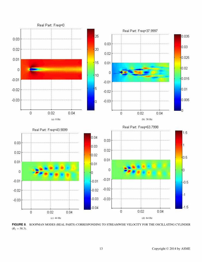
Real parts of various Koopman modes are shown in Figs. 8and 9. In comparison to Fig. 6(b), the larger amplitude oscil-lation results in much different spatial structure near the sta-tionary cylinder von Karman shedding frequency. The modeshown in Fig. 8(b) does not show the organized anti-symmetricstructure of Fig. 6(b). Interestingly, the spatial structure associ-ated with the von Karman shedding mode appears to manifest at64 Hz in Fig. 8(d). Similar spatial structure is exhibited at 44Hz also (although at lower magnitudes). Therefore, the exter-nally forced oscillation has not completely disrupted the shed-ding mode; rather it appears to have been shifted and distributedacross higher frequencies. This is consistent with earlier find-ings on behavior of eigenfunctions of transfer operators througha bifurcation [27].

As shown in Figs. 9(b) and (c), the lower amplitude oscilla-tion case exhibits the von Karman modal structure at frequenciesclose to the stationary cylinder shedding frequency. In addition,

Fig. 9(d) indicates that the mode corresponding to Fig. 6(c) ap-pears to have been shifted to higher frequencies for the oscillat-ing case. Furthermore, it is interesting to note that the mode cor-responding to 132 Hz (not shown) for the large amplitude case re-sembles the spatial structure associated with Fig. 6(c) (i.e. twicethe shedding frequency), while for the small amplitude case the132 Hz mode resembles Fig. 6(d) (i.e. three times the sheddingfrequency).

Static Airfoil and Oscillating Airfoil under DynamicStall

Results are presented for Koopman spectral decompositionsof streamwise velocity for an oscillating NACA 0015 airfoilwith semi-chord b = 0.0675 m, and freestream Mach numberM = 0.3. The pitch oscillation was parameterized as θ0 = 18o

and cases corresponding to θ1 = 0o, θ1 = 2o, and θ1 = 6o wereconsidered. The static pitch angle was selected so that the airfoilwould be well within the separated flow regime. The static airfoilin a deep stall condition provides an analog with the stationarycylinder case in the sense that both exhibit flow behavior charac-teristic of blunt body shedding. Similarly, the airfoil oscillationamplitudes were selected in order to provide comparisons withthe dynamics exhibited by the small and large amplitude cylinderoscillations cases. For θ1 = 6o, the oscillation amplitude is suffi-cient to cause the airfoil to periodically pass above and below thestatic separation angle. In contrast, θ1 = 2o is small enough suchthat the airfoil oscillates at angles that are always greater than thesteady separation angle. Thus, the θ1 = 6o case is analogous tothe large amplitude oscillating cylinder case, while the θ1 = 2o


corresponds to the small amplitude oscillating cylinder. Note thatonly the θ1 = 6o case would be considered dynamic stall sincethe airfoil periodically traverses through separation and reattach-ment. The reduced frequency k = ω1b/U0 was 0.1 – which is arepresentative value for helicopter dynamic stall – correspondsto 24 Hz.

The spectrum for the stationary airfoil (θ1 = 0o) is shown inFig. 10, where it is clear that there is a dominant oscillatory modeat 470 Hz. As shown in Fig. 11(b), this modes corresponds to awake shedding mode. The harmonics of this mode are shownin Figs. 11(c) and (d). As expected, the spatial structure of themode shapes shown in Fig. 11 exhibit strong qualitative simi-larities with those from Fig. 6 for the stationary cylinder case.For instance, both exhibit coherent wake structures shed in analternating pattern for the dominant oscillatory modes. In addi-tion, the progressively smaller spatial wavelengths of the higherharmonics of the shedding mode are evident in Figs. 11(c) and(d), and their stationary cylinder counterparts in Figs. 6(c) and(d) respectively. Perhaps the most important difference betweenthe cylinder and the airfoil is that the statically pitched airfoilhas a leading edge separated shear layer – e.g. Fig. 11(b) – thatextends much further in the streamwise direction before rollingup into wake structures compared to the airfoil trailing edge.One can imagine that as the airfoil static angle of attack goesto θ0 = 90o and transitions from a streamlined shape to a bluntbody, the shear layers from the leading and trailing edges wouldpenetrate similar streamwise distances before rolling up into co-herent wake structures.

Figure 12 shows the spectra for the θ1 = 6o and θ1 = 2o

oscillation cases. Note that the oscillation frequency (24 Hz) isan order of magnitude lower than the dominant fluid dynamicscale associated with the stationary airfoil shedding mode (470Hz). As mentioned previously, the oscillating cylinder frequen-cies were also an order of magnitude lower than the dominantfluid dynamic mode in order to facilitate comparison between thetwo systems. Just as in the oscillating cylinder case, the oscilla-tion induces broadening of the spectrum compared to the discretecase shown in Fig. 10 for the stationary airfoil. These resultssuggest that the underlying nonlinear dynamics associated withdynamic stall exhibit features similar to the oscillating cylindercanonical system, and that oscillation through bifurcation mayinduce the spectral broadening in dynamic stall.

Selected Koopman modes for both oscillation amplitudesare compared in Fig. 13. The static airfoil wake shedding (bi-furcation) mode has not been completely destroyed; rather, it ap-pears to have been distributed across range of frequencies justas in the oscillating cylinder cases. For the low amplitude os-cillating airfoil case, Figs. 13(c) and (e) show that the station-ary airfoil wake shedding mode has been spread across frequen-cies in the vicinity of 400 Hz. Similarly, the distributed spectralcontent centered about approximately 354 Hz in Fig. 12(b) forthe large amplitude oscillation case corresponds to a mode with

features similar to the shedding mode as shown in Fig. 13(d).Furthermore, at 421 Hz in Fig. 13(f), the coherency of the shed-ding mode spatial character begins to break down into a morechaotic structure, which appears to be analogous to the behaviorobserved for the large amplitude oscillating cylinder case shownin Fig. 8(b). In addition to the spectral broadening shown inFig. 12, the preservation and distribution of the bifurcation modepresented in Fig. 13 strengthens support for the hypothesis thatdynamic stall exhibits dynamics due to periodic passage througha Hopf bifurcation parameter.

For both oscillating airfoil cases, Fig. 12 indicates that a sig-nificant portion of the dynamically relevant features are shiftedbelow 400 Hz. Interestingly, the oscillating airfoil case exhibitsbroadening at frequencies lower than the steady airfoil sheddingmode, whereas the oscillating cylinder spectral content tended tobe above the stationary cylinder shedding frequency. One hy-pothesis is that the cylinder involves one dominant mode (and itsharmonics), while the oscillating airfoil cases involve the interac-tion of two coherent modal features – the leading edge separatedshear layer and the blunt-body type wake structures. As indi-cated in Figs. 13(a) and (b), these lower frequency modes exhibita strongly coherent leading edge shear layer in addition to coher-ent wake structures. It is possible that this interaction betweentwo strongly coherent features induces some differences that arenot captured by the canonical cylinder system. This is a subjectof ongoing study.

CONCLUSIONSAn initial treatment of nonlinear dynamics due to oscil-

lation through bifurcation using Koopman modal analysis waspresented. Two-dimensional CFD simulations of the canoni-cal streamwise oscillating cylinder problem were studied in or-der to consider a physical realization of a high-dimensional dy-namic system characterized by externally forced periodic pas-sage through a bifurcation parameter. Koopman modal analysiswas used to show that a more continuous spectrum associatedwith the oscillating cylinder is induced compared to the station-ary cylinder case. The emergence of more chaotic dynamics(i.e. continuous spectrum) is known to be a feature of a sys-tem in which a Hopf bifurcation critical value is traversed in anoscillatory manner, while a discrete spectrum is expected of asystem operating well above the critical value. The spectral fea-tures identified using Koopman decompositions of the oscillatingcylinder were compared to Fourier decompositions of the trans-verse velocity components corresponding to a pitch oscillatingairfoil that induces dynamic stall. The spectral characteristics ofthe two systems exhibit similar frequency broadening featuresdue to the externally forced oscillations. Therefore, the nonlin-ear dynamics associated with dynamic stall appear to have stronglinkages to the effects of oscillating through a bifurcation criti-cal value. This new insight into dynamic stall is enabled by the


Koopman spectral analysis technique.

ACKNOWLEDGMENTSupport for M. Fonoberova, S. Loire, and I. Mezic under

U.S. Army Research Office project W911NF-14-C-0102, andU.S. Air Force Office of Scientific Research project FA9550-12-1-0230 are gratefully acknowledged.

REFERENCES[1] McCroskey, W., 1982. “Unsteady airfoils”. Annual Review

of Fluid Mechanics, 14(1), pp. 285–311.[2] Ham, N. D., and Young, M. I., 1966. “Torsional oscillation

of helicopter blades due to stall”. Journal of Aircraft, 3(3),pp. 218–224.

[3] Carta, F. O., 1967. “An analysis of the stall flutter instabilityof helicopter rotor blades”. Journal of American HelicopterSociety, 12(4), pp. 1–18.

[4] Visbal, M. R., 2011. “Numerical investigation of deep dy-namic stall of a plunging airfoil”. AIAA Journal, 49(10).

[5] Dowell, E. H., 1996. “Eigenmode analysis in unsteadyaerodynamics: Reduced-order models”. AIAA Journal,34(8).

[6] Huerre, P., and Monkewitz, P., 1990. “Local and globalinstabilities in spatially developing flows”. Annual Reviewof Fluid Mechanics, 22(1), pp. 473–537.

[7] Mulleners, K., and Raffel, M., 2012. “The onset of dynamicstall revisited”. Experiments in Fluids, 52.

[8] Glaz, B., Friedmann, P. P., Liu, L., Cajigas, J. G., Bain,J., and Sankar, L. N., 2013. “Reduced-order dynamic stallmodeling with swept flow effects using a surrogate-basedrecurrence framework”. AIAA Journal, 51(4), pp. 910–921.

[9] Mezic, I., 2005. “Spectral properties of dynamical systems,model reduction and decompositions”. Nonlinear Dynam-ics, 41(1), pp. 309–325.

[10] Mezic, I., 2013. “Analysis of fluid flows via spectral prop-erties of the koopman operator”. Annual Reviews of FluidMechanics, 45, pp. 357–378.

[11] Rowley, C., Mezic, I., Bagheri, S., Schlatter, P., and Hen-ningson, D., 2009. “Spectral analysis of nonlinear flows”.Journal of Fluid Mechanics, 641(1), pp. 115–127.

[12] Budisic, M., and Mezic, I., 2012. “Applied koopmanism”.Chaos, 22.

[13] Koopman, B., 1931. “Hamiltonian systems and transfor-mation in Hilbert space”. Proceedings of the NationalAcademy of Sciences of the United States of America,17(5), p. 315.

[14] Susuki, Y., and Mezic, I., 2012. “Nonlinear koopmanmodes and a precursor to power system swing instabilities”.

Power Systems, IEEE Transactions on, 27(3), pp. 1182–1191.

[15] Schmid, P., 2010. “Dynamic mode decomposition of nu-merical and experimental data”. Journal of Fluid Mechan-ics, 656(1), pp. 5–28.

[16] Mariappan, S., Gardner, A., Richter, K., and Raffel, M.,2013. “Analysis of dynamic stall using dynamic mode de-composition technique”. 31ST AIAA Applied Aerodyan-mics Conference.

[17] Sreenivasan, K. R., Strykowski, P. J., and Olinger, D. J.,1987. “Hopf bifurcation, landau equation and vortex shed-ding behind circular cylinders”. In Proc. Forum UnsteadySeparation, ed. K. N. Ghia, 52.

[18] Bagheri, S., 2013. “Koopman-mode decomposition of thecylinder wake”. Journal of Fluid Mechanics, 726, pp. 596–623.

[19] Provansal, M., Mathis, C., and Boyer, L., 1987. “Benard-von karman instability: Transient and forced regimes”.Journal of Fluid Mechanics, 182, pp. 1–22.

[20] Leontini, J. S., Jacono, D. L., and Thompson, M. C., 2013.“Wake states and frequency selection of a streamwise os-cillating cylinder”. Journal of Fluid Mechanics, 730,pp. 162–192.

[21] Rowley, C., Colonius, T., and Murray, R., 2004. “Modelreduction for compressible flows using POD and Galerkinprojection”. Physica D: Nonlinear Phenomena, 189(1),pp. 115–129.

[22] Temam, R., 1997. Infinite-dimensional dynamical systemsin mechanics and physics. Springer-Verlag.

[23] Singh, R., and Manhas, J., 1993. Composition operators onfunction spaces. No. 179. North Holland.

[24] Gaspard, P., 2005. Chaos, scattering and statistical me-chanics. Cambridge Univ. Press.

[25] Schmid, P., and Sesterhenn, J., 2008. Dynamic modedecomposition of numerical and experimental data. 61stAnnual Meeting of the APS Division of Fluid Dynamics,November.

[26] Vance, W., Tsarouhas, G., and Ross, J., 1989. “Universalbifurcation structures of forced oscillators”. Progress ofTheoretical Physics Supplement, 99, pp. 331–338.

[27] Junge, O., Marsden, J. E., and Mezic, I., 2004. “Uncer-tainty in the dynamics of conservative maps”. 43rd IEEEConference on Decision and Control, 2(369-377).


(a) 0 Hz (b) 39 Hz

(c) 78 Hz (d) 118 Hz

FIGURE 6. KOOPMAN MODES (REAL PARTS) CORRESPONDING TO STREAMWISE VELOCITY FOR THE STATIONARY CYLINDER.


(a) Re1 = 35

(b) Re1 = 5.83

FIGURE 7. STREAMWISE VELOCITY COMPONENT SPECTRA FOR FLOW OVER AN OSCILLATING CYLINDER; FREQUENCIES IN Hz


(a) 0 Hz (b) 38 Hz

(c) 44 Hz (d) 64 Hz

FIGURE 8. KOOPMAN MODES (REAL PARTS) CORRESPONDING TO STREAMWISE VELOCITY FOR THE OSCILLATING CYLINDER(R1 = 58.3).


(a) 0 Hz (b) 38 Hz

(c) 44 Hz (d) 89 Hz

FIGURE 9. KOOPMAN MODES (REAL PARTS) CORRESPONDING TO STREAMWISE VELOCITY FOR THE OSCILLATING CYLINDER(R1 = 5.83).


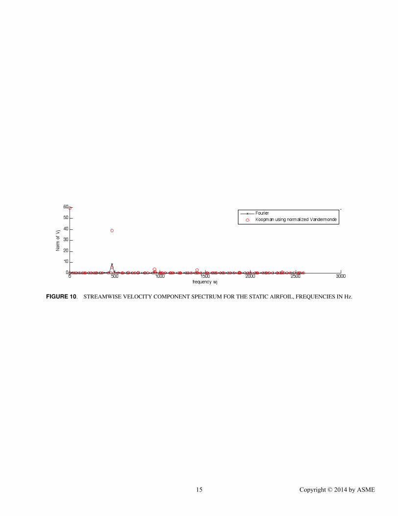
FIGURE 10. STREAMWISE VELOCITY COMPONENT SPECTRUM FOR THE STATIC AIRFOIL, FREQUENCIES IN Hz.


(a) 0 Hz (b) 470 Hz

(c) 939 Hz (d) 1410 Hz

FIGURE 11. KOOPMAN MODES (REAL PARTS) CORRESPONDING TO STREAMWISE VELOCITY FOR THE STATIONARY AIRFOIL.


(a) θ1 = 2o

(b) θ1 = 6o

FIGURE 12. STREAMWISE VELOCITY COMPONENT SPECTRA FOR PITCH OSCILLATING AIRFOILS; FREQUENCIES IN Hz


(a) θ1 = 2o (b) θ1 = 6o

(c) θ1 = 2o (d) θ1 = 6o

(e) θ1 = 2o (f) θ1 = 6o

FIGURE 13. KOOPMAN MODES (REAL PARTS) CORRESPONDING TO STREAMWISE VELOCITY FOR THE OSCILLATING AIRFOIL.18 Copyright © 2014 by ASME

Analysis of Fluid Motion in Dynamic Stall and Forced ...

Documents

Transcript of Analysis of Fluid Motion in Dynamic Stall and Forced ...