University of PennsylvaniaScholarlyCommons

Technical Reports (CIS) Department of Computer & Information Science

January 1990

Analysis of Error Control and Congestion ControlProtocolsAmarnath MukherjeeUniversity of Pennsylvania

Follow this and additional works at: http://repository.upenn.edu/cis_reports

University of Pennsylvania Department of Computer and Information Science Technical Reports No. MS-CIS-90-87.

This paper is posted at ScholarlyCommons. http://repository.upenn.edu/cis_reports/352For more information, please contact libraryrepository@pobox.upenn.edu.

Recommended CitationAmarnath Mukherjee, "Analysis of Error Control and Congestion Control Protocols", . January 1990.

Analysis of Error Control and Congestion Control Protocols

AbstractThis thesis presents an analysis of a class of error control and congestion control protocols used in computernetworks.

We address two kinds of packet errors: (a) independent errors and (b) congestion-dependent errors. Ourperformance measure is the expected time and the standard deviation of the time to transmit a large message,consisting of N packets.

The analysis of error control protocols. Assuming independent packet errors gives an insight on how the errorcontrol protocols should really work if buffer overflows are minimal. Some pertinent results on theperformance of go-back-n, selective repeat, blast with full retransmission on error (BFRE) and a variant ofBFRE, the Optimal BFRE that we propose, are obtained.

We then analyze error control protocols in the presence of congestion-dependent errors. We study theselective repeat and go-back-n protocols and find that irrespective of retransmission strategy, the expectedtime as well as the standard deviation of the time to transmit N packets increases sharply the face of heavycongestion. However, if the congestion level is low, the two retransmission strategies perform similarly. Weconclude that congestion control is a far more important issue when errors are caused by congestion.

We next study the performance of a queue with dynamically changing input rates that are based on implicit orexplicit feedback. This is motivated by recent proposals for adaptive congestion control algorithms where thesender's window size is adjusted based on perceived congestion level of a bottleneck node. We develop aFokker-Planck approximation for a simplified system; yet it is powerful enough to answer the importantquestions regarding stability, convergence (or oscillations), fairness and the significant effect that delayedfeedback plays on performance. Specifically, we find that, in the absence of feedback delay, a linear increase/exponential decrease rate control algorithm is provably stable and fair. Delayed feedback, however, introducescyclic behavior. This last result not only concurs with some recent simulation studies, it also expoundsquantitatively on the real causes behind them.

CommentsUniversity of Pennsylvania Department of Computer and Information Science Technical Reports No. MS-CIS-90-87.

This technical report is available at ScholarlyCommons: http://repository.upenn.edu/cis_reports/352

ANALYSIS OF ERROR CONTROL AND CONGESTION CONTROL PROTOCOLS

AMARNATH MUKHERJEE

A thesis submitted in partial fulfillment of the requirements for the degree of

Doctor of Philosophy Computer Sciences

at the UNIVERSITY OF WISCONSIN - MADISON

1990

Abstract

This thesis presents an analysis of a class of error control and congestion

control protocols used in computer networks.

We address two kinds of packet errors: (a) independent errors and (b)

congestion-dependent errors. Our performance measure is the expected time

and the standard deviation of the time to transmit a large message, consisting

of N packets.

The analysis of error control protocols assuming independent packet

errors gives an insight on how the error control protocols should really work

if buffer overflows are minimal. Some pertinent results on the performance of

go-back-n, selective repeat, blast with full retransmission on error (BFRE)

and a variant of BFRE, the Optimal BFRE that we propose, are obtained.

We then analyze error control protocols in the presence of congestion-

dependent errors. We study the selective repeat and go-back-n protocols and

find that irrespective of retransmission strategy, the expected time as well as

the standard deviation of the time to transmit N packets increases sharply

the face of heavy congestion. However, if the congestion level is low, the two

retransmission strategies perform similarly. We conclude that congestion

control is a far more important issue when errors are caused by congestion.

We next study the performance of a queue with dynamically changing

input rates that are based on implicit or explicit feedback. This is motivated

by recent proposals for adaptive congestion control algorithms where the

sender's window size is adjusted based on perceived congestion level of a

bottleneck node. We develop a Fokker-Planck approximation for a simplified

system; yet it is powerful enough to answer the important questions regarding

stability, convergence (or oscillations), fairness and the significant effect that

delayed feedback plays on performance. Specifically, we find that, in the

absence of feedback delay, a linear increase/exponential decrease rate control

algorithm is provably stable and fair. Delayed feedback, however, introduces

cyclic behavior. This last result not only concurs with some recent simulation

studies, it also expounds quantitatively on the real causes behind them.

Acknowledgments

I most sincerely acknowledge:

a) Professors Larry Landweber and John Strikwerda for teaching me all

the good stuff, caring about me and my work and for all the patience

when I goofed,

b) Professor Mary Vernon, for her quality help all along, including, working

on my slides into the wee-hours of the morning,

c ) Professors Bart Miller and Tom Leonard, for most graciously agreeing

to be in my committee,

d) Professor Miron Livny, for providing me his DeNet simulation tool,

e) Sheryl Pomraning, Laura Cuccia and Lorene Webber, for being ever so

helpful and nice,

f ) Cheng Song and Mitch Tasman, for being wonderful officemates,

g) my friends, in reverse alphabetic order: Vikram/Sarita, Tsuei, Sriram

Vajapeyam, Shahram, Scott/Lisa, Rustam, Prasad, Parikshit, Osty,

Narendran, George Bier, Gautam/Moneka, Deshpande, Chinmoy/

Sumita Roy and family, Basu, Atul Parekh, Arun/Purabi Datta and

family, Argha, Ananda/Mousumi,

h) my chess buddies, Bill Olk, Bill Arvola, Dean Olson, Guy Hoffman,

Joseph Albert, Karl Zanguerle, Larry Butler, Marc Ingeneso and Senthil

Kumax,

i) IBM, for providing me financial support during 1989-90,

j) the Computer Sciences Department, the Memorial Union Terrace, and

Madison city in general, for making these years most wonderful.

I am also deeply indebted to my parents and my family for their love, un-

derstanding and support.

CONTENTS

. . . . . . . . . . . . . . . . . . . . . . . . 1 Introduction 1 . . . . . . . . . . . . 1.1 Problem Statement and Motivation 1

. . . . . . . . . 1.2 Overall Approach and Summary of Results 4 . . . . . . . . . . . . . . . . . . . . . 1.3 Thesis Outline 6

. . . . . . . . . . . . . . . . . . . . . . . 2 Related Work 10 . . . . . . . . . . . . . . . . . . . . . . . . . 2.1 Outline 10

. . . . . . . . . . . . . . . . . 2.2 Error Control Protocols 10 . . . . . . . . . . . . . . . . . . . . . 2.2.1 Background 10

. . . . . . . . . . . . . . . 2.2.2 Basic Protocol Definitions 11 . . . . . . . . . . . . . . 2.2.3 Queueing Analysis Results 12

. . . . . . . . . . . . . . . . . . . . 2.2.3.1 Go-back-n 13 . . . . . . . . . . . . . . . . 2.2.3.2 Stutter g-back-n 15

. . . . . . . . . . . . . . 2.2.3.3 Selective repeat protocol 16 . . . . . . . . . 2.2.4 Maximum Channel Throughput Results 18

. . . . . . . . . 2.2.4.1 Bruneel and Moeneclaey Protocol 19

2.3 Congestion Control, Congestion Avoidance and Flow Control . 22 . . . . . . . . . . . . . . . . . . . . 2.3.1 Preliminaries 22

. . . . . . . . . . . . . . . 2.3.2 What causes congestion? 23 . . . . . . . . . . . . . . . . . . 2.3.3 Proposed Solutions 24

3 Evaluation of Error Recovery Protocols with Independent . . . . . . . . . . . . . . . . . . . . . . . . Packet Errors 29

. . . . . . . . . . . . . . . . . . . . . . 3.1 Introduction 29

. . . . . . . . . . . . . . . . . . . . . . 3.2 Preliminaries 31 . . . . . . . . . . . . . . . . . . . . . 3.2.1 TheModel 31

. . . . . . . . . . . . . . . . . . . . 3.2.2 The Protocols 35 . . . . . . . . . . . . 3.3 Go-Back-N Retransmission Strategy 36

. . . . . . . . . . . . . . . . . . . . . . 3.3.1 Notation 36

. . . . . . . . . . . . . . . . . . . . . . 3.3.2 Analysis 37

. . . . . . . . . . . . . . . . . . . . . 3.4 Selective Repeat 41 . . . . . . . . . . . . . . . . . . . 3.4.1 Distribution of X 43 . . . . . . . . . . . . . . . . . . . 3.4.2 Distribution of Y 44

. . . . . . . . . . . . . . . . . . . . 3.5 Numerical Results 46 . . . . . . . . . . . . . . . . . . 3.6 Optimal Blast Protocol 48

. . . . . . . . . . . . . 3.7 Generalized Analysis of Go-back-n 55

. . . . . . . . . . . . . . . . 3.8 Summary and Conclusions 57 . . . . . . . . . . . . . . . . . . 4 Go-back-n with Windows 59

. . . . . . . . . . . . . . . . . . . . . . 4.1 Introduction 59 . . . . . . . . . . . . . . . . . . . . 4.2 Petri Net Models 59

. . . . . . . . . . . . . . . . . . . . . . . . 4.3 Analysis 62

. . . . . . . . . . . . . . . . . 4.3.1 Analysis of Model I 62

. . . . . . . . . . . . . . . . . 4.3.2 Analysis of Model II 63

. . . . . . . . . . . . 4.3.3 Comparison of the two methods 64 . . . . . . . . . . . . . . . . . . . . . . 4.4 Conclusions 67

5 Analysis of Error Control Protocols with . . . . . . . . . . . . . . . . . Congestion-Dependent Errors 69

. . . . . . . . . . . . . . . . . . . . . . 5.1 Introduction 69

. . . . . . . . . . . . . . . . . . . . . . 5.2 The Model 70

. . . . . . . . . . . . . . . . . 5.3 go-back-n protocol model 76

. . . . . . . . . . . . . 5.4 Selective repeat protocol analysis 80

. . . . . . . . . . . . . . . . . . . . 5.5 Numerical Results 84 . . . . . . . . . . . . . . . . . . . . . . 5.6 Conclusions 89

. . . . . . . 6 Analysis of Dynamic Congestion Control Protocols 91 . . . . . . . . . . . . . . . . . . . . . . 6.1 Introduction 91

. . . . . . . . . . . . . . . . . . . . . . . . . 6.2 Model 92

6.3 Fokker-Planck approximation for queue with feedback control . 94

. . . . . . . . . . . . . . . 6.4 Properties of Algorithm 6.2 97 . . . . . . . . . . . . . . . . . . . . 6.5 Multiple Sources 105

. . . . . . . . . . . . . . . . . 6.6 Effect of feedback delay 108 . . . . . . . . . . . . . . . 6.7 Summary and conclusions 110

. . . . . . . . . . . . . . . . . . . . . . 7 Futurework 112

7.1 Introduction . . . . . . . . . . . . . . . . . . . . . 112

. . . . 7.2 Congestion control in high speed. wide area networks 112

. . . 7.3 Fokker-Planck analysis of feedback control with delay 118

Bibliography . . . . . . . . . . . . . . . . . . . . . . . . 119 Appendices

Appendix 3.A . . . . . . . . . . . . . . . . . . . . . . . 126

Appendix 3.B . . . . . . . . . . . . . . . . . . . . . . . 129

Appendix 5.A . . . . . . . . . . . . . . . . . . . . . . . 133

Chapter 1

Introduction

1 .I. ' Problem Statement and Motivation

This thesis presents an analysis of a class of protocols used in computer

networks. The analysis of these protocols is important because

a) it gives an estimate of the performance of these protocols that is other-

wise hard to obtain,

b) it quantifies the relative importance of different performance issues and

c) it identifies quantitatively the cause of any undesirable behavior.

As an example, consider the computer network1 shown in Figure 1.1.

The network consists of nodes which are interconnected with channels. Each

node serves as a switching element that routes packets from one of several

inputs to one of several outputs. It has limited buffering capabilities to deal

with sudden bursts in traffic. Users, located outside of this network in hosts

communicate with each other through this network. They do so by means of

predefined protocols, which specify the rules of interaction between two semi-

autonomous units. There is an entire gamut of protocols that are defined

for computer communication. These provide different services like reliable

data delivery, directory service, multicasting, etc. The quality of service that

the protocol provides may vary depending upon the perceived importance of

that service. For instance, a protocol could provide reliable and sequential

delivery of packets as in X.25, or it could make only a best effort at delivering

individual packets as in IP. In the latter case, the sender and the receiver

may agree on a protocol for error recovery at a higher level. Protocols may

or rather its queueing network model

Figure 1.1. An example computer network.

also specify a fixed or variable rate of transmission or the maximum number

of packets (the window size) that the sender could have outstanding at any

time before receiving an acknowledgment from the receiver. These protocols

are called flow control and congestion control protocols. Briefly, flow con-

trol attempts to alleviate mismatch in speeds between the end-points while

congestion control protects the network elements from being overrun by fast

transmitters. It is often easy to devise a protocol but di f icul t to estimate

or ver2fy how it will perform. A further complication arises from the fact

that a protocol may also have side eflects on the performance of other pro-

tocols. Thus a poor congestion control protocol could, for instance, drive

up the error rates artificially to the point where the chosen error recovery

protocol is sub-optimal. It is therefore important to develop methods for

assessing not only the performance of these protocols in isolation, but also

to consider their interactions if necessary, using either analytical techniques

or simulations and experiments.

Protocols create interesting and intriguing phenomena which can be

expressed mathematically and analyzed for their performance. In this thesis,

we apply mathematical analysis to the specific problems of understanding

error control and congestdon control protocols.

Error control protocols, as the name implies, are used to recover from

errors. When some user, say at host A in Figure 1.1, submits a message to

the network to be transmitted to another user, say at host B, the message

is usually split into packets which are transmitted over the network and

reassembled at the other end. A packet in transit encounters one or more

channels, (e.g., satellite, copper wire or optical fiber), and nodes (or routers) ,

which route the packet to the destination. These intermediate elements can

induce errors in the packet in that either the packet could get garbled, or

dropped altogether. The former is usually due to random electrical noise

in the channels while the latter is due to buffer overruns at the nodes and

is caused by contention for resources, a phenomenon often referred to as

congestion.

Protocols that are implemented to recover from packet errors are called

error control protocols; those that attempt to alleviate congestion are called

congestdon control protocols. With respect to performance, their interaction

is closely related. The overall end-to-end performance for a user depends on

how well a combination of the two protocols performs. The use of fiber optic

technology has significantly decreased network errors in channels; hence the

load on the error control protocol depends heavily on the success (or fail-

ure) of the congestion control protocol because the latter affects congestion-

related losses. Conversely, an error control protocol could also aggravate

congestion in the network, for example, by introducing a large number of

retransmitted packets. An analysis of end-to-end user performance m u s t

therefore s tudy these two protocols in un i son rather t h a n in isolatzon. Pre-

vious work has, however, not addressed these two issues simultaneously. In

our study, we explicitly address errors that are caused by congestion.

A related and perhaps more important problem in congestion control

is the transient analysis of dynamic congestion control protocols [RaJa 88,

Jac 881. These protocols adjust the sender's window size based on perceived

congestion level of a bottleneck node. To analyze their performance, one

needs to study the stochastic behavior of a queue with dynamically changing

input rates which are based on feedback. The issues that need investigation

are

a) how quickly does the system adapt to changing environments?

b) does it stabilize or show cyclic behavior?

c) is the protocol fair?

d) how do the system parameters (like delay, multiple hops, other compet-

ing users, etc.) change any of the above?

Precise answers to these questions that either support or point to flaws

in common intuition are certainly worthwhile, and are the subject of our

study.

1.2. Overall Approach and Summary of Results

Our study focuses on the statistics of the t i m e t o comple te a mul t i -

packet end- to-end message transfer . The measures used in previous analyses

on error control protocols were m a x i m u m channel throughput or queue length

characteris t ics a t t h e sender , given assumptions of packet arrival rates and

distributions [AnPr 86, BrMo 86, ToWo 79, MoQiRa 871. For a user who is

interested in accessing files, or in remote procedure calls over a network, how-

ever, end- to-end performance is a more relevant measure. Hence, we choose

the time to successfully transmit a message of N packets as our performance

measure . The only other study that incorporates this performance measure

is one by Zwaenepoel [Zwa 851, who analyzed the stop-and-wait protocol and

blast protocol wi th ful l -retransmission-on-error (BFRE) for a multi-packet

message assuming independent packet errors.

Our first contribution is a theoretical analysis of the go-back-n and se-

lective repeat protocols under the same assumptions as Zwaenepoel's and a

comparative study of these and BFRE in a local area network environment.

We derive expressions for the expectation, variance and the distribution of

time to transmit N-packets using the go-back-n and selective repeat proto-

cols. These are compared to the expressions for BFRE. We conclude that

go-back-n performs almost as well as selective repeat while BFRE is stable

only for a limited range of message sizes and error rates. Since go-back-n

has a simpler state machine than selective repeat, it is therefore the pro-

tocol of choice. We also present a variant of BFRE, the opt imal BFRE, which optimally checkpoints the transmission of a large message. This is

shown to overcome the instability of ordinary BFRE. Moreover, its simple

state machine seems to take full advantage of the low error rates of local

area networks. We further investigate go-back-n by generalizing the analy-

sis to an upper layer transport protocol, which is likely to encounter among

other things, variable delays due to protocol overhead, multiple connect ions,

process switches and operating system scheduling priorities.

Our next contribution is the analysis of error control protocols when

errors are congestion-dependent. Most earlier work assumed statistically in-

dependent packet errors. This is not a very realistic assumption in today's

networks because buffer overruns are the principal source of errors and these

errors are correlated. In fact, it is more likely for an error to occur when one

has already occurred than when none has. We develop models of congestion

which help evaluate the go-back-n and the selective repeat protocols. The

congestion model is based on the empirical evidence2 that in window based

flow control protocols, a connection's loss rates increase monotonically with

the number of packets that it has outstanding in the network.

A third contribution of this research is the theoretical analysis of a class

of congestion control protocols that rely on feedback. These protocols are

adaptive in that they require the end-points to adjust the window size or

the rate of transmission when congestion sets in at some intermediate node.

We develop from first principles, a Fokker-Planck equation for the evolution

of the joint probability density function of queue length and arrival rate at

this node. This approximates the transient behavior of a queue subjected

See Figure 7 in [SSSGJ 881. This particular observation was, however, not made by the authors. Also see the note to Figure 9 in [Jac 881 for further evidence.

to an adaptive rate-control algorithm. It can answer important questions

regarding stability (or oscillations) and fairness of a particular adaptive al-

gorithm as well as the significant effect of delayed feedback on the conclusions.

For instance, in the absence of feedback delay, senders using the Jacobson-

Ramakrishnan-Jain (JRJ) algorithm [Jac 88, RaJa 88,901, (or rather, an

equivalent rate-based algorithm) can be shown to converge to an equilib-

rium. Further, this algorithm is fair in that all the sources sharing this

resource get an equal share if they use the same parameters for adjusting

their rates. The exact share of the resource when the different sources use

different parameters can also be determined from this analysis.

A delay in the feedback information will cause the system to exhibit

oscillatory behavior. These oscillations converge to a limit cycle. If different

sources get the feedback information after different amounts of delay, then

the algorithm can also be unfair, i.e., they do not get equal throughput.

In a simulation study of the same protocol, Zhang observed oscillations in

the queue length at intermediate nodes [Zha 891. She also observed that

connections with larger number of hops received a poorer share of a shared

resource than those with a smaller number of hops. Our analysis not only

concurs with her simulations, it also explains the reasons for the behavior

of the protocols she simulated. The oscillations are due to delay in feedback;

the unfairness is partly due to the larger (feedback) delay suffered by the

longer connections as compared to the shorter ones.

Thesis Outline

Chapter 2 surveys related work in error control and congestion control

protocols. It also has all the relevant definitions. In Chapters 3-5, we study

error control protocols. First, we reduce the degrees of freedom to the case

when errors are statistically independent, the network consists of a single hop

and there are no windowing effects. This study is presented in Chapter 3.

We investigate the performance of the go-back-n protocol, the selective repeat

protocol, the blast protocol w i t h full re t ransmiss ion o n error (BFRE) and a

variant of BFRE which we call the opt imal blast protocol. We find that the

BFRE protocol becomes unstable much faster with respect to message size

than the go-back-n protocol or the selective-repeat protocol. However, since

BFRE has a very simple state machine, it makes other design issues much

simpler and efficient (for example, the network interface design of Kanakia

and Cheriton [KaCh 881). It also seems ideally suited for an environment

where host processing time is a significant amount of the total time, precisely

because the amount of 'work' to be done by the host is reduced. This is the

motivation for our opt imal blast protocol which performs well for both large

and small message sizes.

In Chapter 4, the assumption of infinite windows is removed. The sin-

gle hop network is also generalized to any arbitrary network. Packet errors

are still assumed to be independent of each other. We find that the win-

dow closing effect has a minimal effect on the analysis of go-back-n. The

window-effects and the error-effects are quasi- independent in that they could

be studied separately and the results put back together in an obvious way.

Unfortunately, no such relationship was found to hold for selective repeat.

In Chapter 5, the assumption of independence of packet errors is re-

moved. The errors are congest ion-dependent . We first develop a new con-

ges t ion model , which gives the probability of error as a function of the num-

ber of packets that are outstanding in the network. The congestion model

is incorporated into the protocol models of go-back-n and selective repeat to

yield two separate continuous time Markov processes. Each Markov process

has an initial state corresponding to the beginning of a message transmis-

sion and a h a 1 state corresponding to its end. A transient solution of the

Markov process yields the expected time to transmit an N-packet message

and its variance. We h d that irrespective of retransmission strategy used,

the expected time as well as the standard deviation of the time to transmit

N packets increases sharply if the window size is large in the face of heavy

congestion. However, if the congestion level is low, the two retransmission

strategies perform similarly.

In Chapter 6, we develop a theory for dynamic congestion control algo-

rithms. The algorithm of Jacobson-Ramakrishnan- Jain [Jac 88, FbJa 88,901,

(the 'JRJ'- algorithm) is a special case of this general framework. In the JRJ

algorithm, when congestion is detected (by implicit or explicit feedback), the

window size is decreased multiplicatively. However, when there is no conges-

tion, it is increased linearly - to probe for more bandwidth. While this

seems to be a good adaptive algorithm, it is far from clear as to what val-

ues the parameters for increasing or decreasing the window size should take.

Further, it is not provably clear if the algorithm is fair or stable and if so,

under what circumstances.

To understand the behavior of dynamic congestion control algorithms,

we study the behavior of a queueing system with a time varying input rate.

This rate is adjusted periodically based on some feedback that the transport

endpoint receives about the state of the queue. Let g(X, q) = dX(t, q)/dt be

the rate control algorithm, where X(t) is the input rate at time, t. As an

example, g(.) could be the following function:

where ij is some threshold queue length. This is the rate-equivalent of the

window based JRJ-algorithm (note the linear increase and exponential decay

components ). A transient analysis of this queueing system is difficult. We have ap-

proximated its behavior by a 2-dimensional Fokker-Planck equation. The

result is a second-order partial differential equation for the joint probability

density function f (-) of the queue length and the arrival rate:

where f (t, q, v) is the joint probability distribution of q and v, v(t) = X(t) - p

is the instantaneous mean queue growth rate, p is the instantaneous mean

service rate of the queue and a2 is the variance of queue growth rate. Equa-

tion 1.2 is studied in detail in Chapter 6. There we find that the linear

increase and exponential decrease algorithm given by Equation 1.1 is inher-

ently stable if there is no delay in feedback, i.e., it converges to the correct

value of X = p and threshold queue-length, ij. The effect of the parameter

values Co and Cl are also studied.

Introduction of feedback delay however adds oscillations which settle

down to a l imit cycle, i.e., a cyclic pattern that is constant in the limit. This

cyclic pattern concurs with simulation results by Zhang [Zha 891. The proof

of the existence of a limit cycle, we believe, is a new result. The diameter of

the limit cycle (or equivalently the magnitude of the oscillations) is sensitive

to the parameters Co, C1 and the feedback delay. For instance, for a fixed

Co and feedback delay, a larger C1 increases this diameter. So, while in the

absence of feedback delay, a larger C1 boosts the speed of convergence, in

the presence of delay, it causes wilder oscillations. The size of the oscillations

also increase with Co and feedback delay.

Chapter 2

Related Work

2.1. Outline

This chapter surveys the literature in error control and congestion con-

trol protocols. Since these two issues have been studied independently of each

other in the past, we split this chapter into two major sub-sections. First,

we review related work on error control protocols and then on congestion

control protocols.

2.2. Error Control Protocols

2.2.1. Background

Two error control protocols that we are primarily interested in inves-

tigating are the go-back-n and the selective repeat protocols. In addition,

we shall also consider the Blast protocol with f i l l retransmission o n error

(BFRE) and a variation of this protocol the opta'mal BFRE, which we pro-

pose in Chapter 3. We shall however not consider the stop-and-wait protocol

because it is known to perform poorly [Zwa 851.

In the next few sub-sections, we shall survey previous work on the go-

back-n and the selective repeat protocols. Numerous variants of these two

protocols have been proposed in the literature [Sha 75, Mor 78, LiYu 78, Tow

791. The design of these protocols seems to be an easy task, whereas their

analysis and performance evaluation proves to be very difficult. Nevertheless,

some of them have been analyzed to determine either their queue length

statistics or the m a x i m u m throughput that they can deliver.

The analyses of these protocols have usually assumed packet errors to

be independent of each other [ToWo 79, Tow 79, Kon 80, AnPr 86, BrMo

861. In addition, the roundtrip delay is assumed to be fixed (deterministic)

and the window is assumed to be open at all times.'

Fujiwara et al, [Fu 781, assumed a burst error model, first suggested

by Gilbert [Gil 60],2 to analyze the throughput of go-back-n in conjunction

with forward error correction. However, they show numerical results for

independent errors only and mention that the burst model behaves similarly.

The outline of the rest of Section 2.2 is as follows. We first review pre-

liminary definition~ of the basic go-back-n and the selective repeat protocols.

As mentioned earlier, numerous small variations of these protocols have been

proposed. We discuss interesting results from the literature on these proto-

col variants. The studies that involve queueing analysis are presented first;

those involving throughput analysis are presented next.

2.2.2. Basic Protocol Definitions

Assuming a sliding window flow control, the basic go-back-n and selec-

tive repeat protocols work as follows: When a packet is successfully received

at the receiver, it is always acknowledged (or ACKed) if it is "in-sequence."

In the case of selective-repeat, the receiver may also ACK out of sequence

These assumptions do not reflect the properties of real networks. It has been demonstrated that the roundtrip delay may fluctuate considerably [Jac 881 and the window can therefore close too.

The Gilbert error model is a correlation model for errors in satellite channels based on a two state Markov process. In one state, the probability of error is zero; in the other, it is equal to p. The transition probabilities between these states completely specifies. the error model.

data, but will not deliver them to its 'user' at the receive-end. In both cases,

an error is detected at the sender by either a timer interrupt or a NACK

from the receiver. At this point, if the sender backs up to the first packet

in error, i.e., the first packet that is not yet ACKed, and restarts the trans-

mission, the strategy is referred to as go-back-n [Tan 811. If, on the other

hand, the sender retransmits only those packets which are in error, the strat-

egy is called selective-repeat. In go-back-n, buffering and reassembling of a

message at the receiver is much simpler than in selective-repeat, but at the

potential cost of retransmitting many more packets. Selective repeat on the

other hand, may require large receive buffers if the propagation delay and

window size are large. The go-back-n protocol is not required to have more

than one receive buffer, although it may buffer packets waiting to be sent to

the user.

Almost all previous work has attributed the 'n' in go-back-'n' to be the

number of packets that the sender backs up by (and retransmits) in case of

an error. 'n' is assumed to be a constant in these studies. This makes sense

if the sender is transmitting a full window of packets all the t i m e and the

window size is 'n7. However, since that is not the case in real networks, we

have chosen to ignore this interpretation of 'n'. Instead, we explicitly use the

window size wherever necessary, thereby permitting more realistic scenarios

with variable number of packets in the pipe.

2.2.3. Queueing Analysis Results

In this sub-section, we outline the queueing analyses for go-back-n, the

'stutter' go-back-n [Tow 791, and the selective repeat protocols. The go-back-

n analysis is due to Towsley and Wolf [ToWo 791. The 'stutter go-back-n'

protocol is a modified go-back-n protocol. It was proposed and analyzed by

Towsley [Tow 791. The selective repeat results are due to Konheim [Kon 801

and Anagnastou and Protonataraious [AnPr 861.

Assumptions

( 1) Time is divided into subintervals of duration A, called slots. All

results are normalized with respect to A, i.e., A = 1.

( 2) Packets arrive at the sending multiplexor just prior to the beginning

of each slot. The number of packets which arrive in any slot is given

by the random variable D. These are independent and identically dis-

tributed (i.i.d) with the distribution pk = P[D = k], k = 0,1,2,. - . . The

distribution has mean p~ = E[D], and variance oDZ = E[(D - pD)2].

( 3) The packets are served on a first-come-first-served basis.

( 4) The number of packets queued in the multiplexor at the beginning of

the jth slot is given by Lj. ( 5) The process has been running long enough so that the statistics of

Lj- l and L j are identical. These are therefore replaced by the generic

random variable L. ( 6) The queue has unlimited capacity.

( 7) The roundtrip delay is a fixed number of slots, s.

Analysis

Because of errors in the channel, a packet may be transmitted more than

once. Let Ni be the total number of times that packet i is transmitted (in-

cluding retransmissions). Assuming Ni are i.i.d. random variables, represent

them by N . Let N have a mean p~ and variance a N 2 . To aid the analysis, a

packet is converted into a, so called, 'slacket', on arrival. A slacket is a ficti-

tious quantity which represents the number of slots that will be necessary to

transmit the packet. Let the slacket size be denoted by the random variable

M with mean / A M and variance a M 2 . M and N are related by the equation

M = 1 + ( N - 1)(1 + s ) = N ( l + s ) - s , since the first transmission takes

one slot, but all subsequent retransmissions take (1 + s ) slots each. Thus

and

The mean queue length at the sender for the go-back-n protocol is then given

by (see [ToWo 791 for details):

Results

Towsley and Wolf plot solutions for the expected queue length assum-

ing a Poisson arrival process and a geometric error probability distribution.

Perhaps the most interesting result is the effect of roundtrip delay (s), and

the error probability (p). The queues grow exponentially as p increases. The

performance also gets worse with increasing s, but the effect is much slower.

For actual quantitative results, the reader is referred to the original paper

[To Wo 791.

2.2.3.2. Stutter go-back-n

The protocol

The performance of the go-back-n protocol degrades with higher error

rates and higher roundtrip delays. To improve the performance of go-back-

n, Towsley [Tow 791 proposes the 'stutter' go-back-n protocol, which is the

original go-back-n with the following modification: during periods when the

channel would normally be idle under go-back-n, the sender repeatedly trans-

mits the last unacknowledged packet, if any, residing in the queue. Towsley

derives the queue length statistics for this protocol, along with that of an

'idealized' retransmission protocol, which in some sense represents the upper

bound on the performance.

The stutter go-back-n protocol has some complications that need clar-

ification. A packet, say i, that has been repeatedly transmitted when the

channel was idle may have several ACKs/NACKs return in consecutive slots.

Assume that there is at least one other packet behind it in the queue now.

Packet i, which is at the head of the queue, should only be retransmitted

if all the acknowledgment packets are NACKs. The sender therefore needs

to keep track of the number of repeated transmissions of a packet and the

number of acknowledgments (ACKs and NACKs) that have returned. No-

tice that if we allow acknowledgment losses, this tracking method fails. The

stutter go-back-n protocol is also not very effective in environments where

errors are congestion-related; unnecessary multiple transmissions of the same

packet in a congested network is highly undesirable.

Assumptions

The assumptions for the analysis of this protocol are the same as that

for the go- back-n protocol discussed earlier.

Analysis

The analysis of this protocol is cumbersome and the formulae give lit-

tle intuitive insight. The methodology however, is similar to the go-back-n

analysis of Towsley and Wolf [ToWo 791. We therefore refer the reader to

[Tow 791 for the detailed analysis.

Results

At low utilizations and/or low error rates, stutter go-back-n cannot im-

prove much over go-back-n because there is not much queueing at these loads.

For very high utilizations, stutter go-back-n cannot not improve much over

go-back-n either, because idle channel bandwidth is hard to come by. How-

ever, for moderately utilized systems and high error rates, stutter go-back-n

improves considerably over go-back-n. For instance, if s = 10,p = 0.1, p =

0.6, (where p is the utilization), the average delay as compared to normal

go-back-n is reduced by 20%. If s = 20, the average delay is reduced by

30%. For s = 10,p = 0.5, p = 0.6, the difference is more than 50%. Notice

the large values of s and p in these examples. It is only for such parameter

values that go-back-n performs poorly.

2.2.3.3. Selective repeat protocol

The results here are due to Anagnostou and Protonotarious [AnPr 861

and Konheim [Kon 801.

Assumptions

( 1) The system is a slotted multiplexor as in the earlier analyses.

( 2) The packet arrival process is the same as that in [ToWo 791 and [Tow

791.

( 3) Transmission errors are independent of each other.

( 4) The queue at the sender has unlimited capacity.

( 5) The roundtrip delay is a constant, denoted by s. Also, if a packet is

transmitted at time m, then either an ACK or a NACK is received in

the slot (m + s - 1,m + s).

( 6) At the beginning of a slot, the first packet in the queue is transmitted,

unless a NACK arrives for an earlier packet in the previous slot. In the

latter case, the packet in error is transmitted. This is the property of

the selective repeat protocol.

Analysis

The analysis of the selective repeat protocol turns out to be considerably

more complex than that of go-back-n. The resulting solutions are algorithmic

in nature. We briefly outline the method of analysis.

The basic idea is to use a discrete time Markov process which describes

the state of the system at any time t ( t is an integer). The state of the system

that is adopted by both [Kon 801 and [AnPr 861 is

where Q(t) = queue length at t + 1, and

1, if a transmission was attempted at t - i + 1, ri(t) = 0, otherwise

The next step is to determine the state transition matrix for the process.

One has to account for the arrivals in the current slot. This will affect Q(t) .

Depending upon whether or not a transmission has taken place s time units

earlier (i.e., if r,(t) = 1 or 0, respectively), there may be an ACKINACK

returning, or nothing at all. Also, since only one packet is transmitted in a

slot, at most one ACKINACK may return in a slot. This, coupled with the

probability of error gives another set of transitions. If no NACK arrives and

Q(t) > 0, then a new transmission is attempted. Note that r; shifts once to

the right and rl is determined by whether or not a transmission is attempted

in the current slot. The state transition matrix is thus completely specified.

Assuming that a steady state is finally reached, the Markov chain de-

scribed above is analyzed (algorithmically) in a standard way to determine

the steady state probabilities. Summing over all possible vectors (rl , . - . , r,),

and a value of queue length, say q, gives the steady state probability distri-

bution of the queue length, P[Q = q] . The mean queue length is then easily

obtained.

Results

The principal results that are presented are curves for the mean queue*

length versus packet error rate for different interarrival times. The interar-

rival times are assumed to be geometrically distributed. As expected, the

curves show poorer performance for higher arrival rates and higher error

probabilities.

2.2.4. Maximum Channel Throughput Results

This set of studies deals with determining the maximum channel

throughput that is obtainable from a given error control protocol. Various

subtle variations of the go-back-n protocol have been proposed, see for ex-

ample [BrMo 86, Bir 81, LiYu 80, Mor 78, Sha 751. The proposal by Bruneel

and Moeneclaey [BrMo 861 is the most general protocol. The authors of that

paper also argue that it is the best. We concur with that view for the case

when errors are independent. (For congestion dependent errors, this proto-

col will need re-evaluation). We discuss the results of this paper in detail.

The other protocols are inferior and we only compare them briefly with the

Bruneel and Moeneclaey protocol.

2.2.4.1. Bruneel and Moeneclaey Protocol

The protocol

The major modification to the go-back-n protocol that Bruneel and

Moeneclaey propose is to transmit multiple copies of each data packet instead

of a single copy. The tradeoff here is between the cost of not transmitting

a new packet in the next slot versus that of finding out that an error has

occurred after a roundtrip delay and retransmitting all over again. For high

network error rates it may be worthwhile to send multiple copies of the data

so that at least one of them reaches correctly. The performance improvement

may be significant for large roundtrip delays. Bruneel and Moeneclaey derive

the optimal number of packets that should be transmitted in each 'cycle' to

maximize throughput. This value is of course dependent on the packet error

probability and the roundtrip delay.

Assumptions

( 1) Packet errors are independent of each other; let p be the packet error

probability.

( 2) All ACK/NACK messages are received error free at the transmitter.

( 3) roundtrip delay is fixed and is equal to s.

( 4) All transmissions of a packet, say i, that were undone by an error

in an earlier packet are ignored for analysis purposes. Thus packet i is

considered to be transmitted for the first time if the previous transmis-

sion of packet i - 1 is successful. At this time, the protocol requires that

mo copies of packet i be transmitted. If all the copies are in error, a re-

transmission cycle is triggered and now ml copies are to be transmitted;

if that fails too, mz copies are to be transmitted and so on. The process

is repeated until a positive acknowledgment for at least one copy of the

packet is received.

Analysis and Results

( 1) Let the optimum value of m j be mj*. Then it is first shown that mO* = ml* = . . . = mj* =, say, m*. The intuition behind this is that,

since packet errors are independent and roundtrip delay is fixed, there

is no difference between any two different (re)transmission cycles.

( 2) m* is determined as follows. Consider the function c(p, s) given by

Also, let 7iz be such that

i.e., m minimizes the expression on the right hand side. Then the opti-

mal value, m*, is given by

00, if c(p, s) < 0, m* = { any number 2 s , if c(p, s) = 0,

7% if c(p, s) > 0.

A consequence of this result is that the curve c(p,s) = 0 divides the

(p, s) plane into two regions, one where c(p, s) > 0 and the optimum is

riz, and the other where c(p,s) < 0 and the optimum is m* = m . When

m* = m , the idea is to keep transmitting the same packet until an

ACK is received for it. The (p, s) diagram (not reproduced here) shows

that for low error rates and low roundtrip delays, m* = 1. However,

as the error rate and the roundtrip delay increases, the value of m*

increases, albeit slowly. Thus, the original go-back-n is optimal only in

a small region of the (p, s) plane. Fortunately, this also happens to be

the region where most networks operate (see the curves in [BrMo 861).

Let us next review (and compare) some of the other modifications that

have been proposed. Shastry [Sha 751 suggests a modified go-back-n protocol

which works as follows: until an error is detected, only a single copy of each

packet is transmitted as in go-back-n; in case of an error however, the packet

in error is transmitted repeatedly until a positive ACK is received for it.

Restated in the Bruneel and Moeneclaey framework, mo = 1 and ml = co.

Clearly this is suboptimal because Bruneel and Moeneclaey show that the

optimal value must be the same across all retransmission cycles, assuming of

course independent packet errors. Network errors are however, bursty and

Shastry's protocol may perform well in practical situations.

Birrel's retransmission scheme, [Bir 811, is also a special case of the

general proposal of Bruneel and Moeneclaey. The m>s are chosen equal to

some common value n less than s. Notice that this cannot be optimal for

the region c(p, s ) < 0, where the optimal value is m* = co.

The selective repeat protocol may outperform the optimal go-back-n

strategy for high error rates and large roundtrip delays.

This concludes our discussion of the literature on error control strategies.

2.3. Congestion Control, Congest ion Avoidance and Flow Control

Preliminaries

" Congestion control is concerned with allocating the resources in a net-

work such that the network can operate at an acceptable performance level

when the demand exceeds or is near the capacity of the network resources"

[Jai 901. The algorithms must address fair resource sharing, buffer over-

runs and large queues at intermediate nodes of the network. Flow control

protocols are similar to congestion control protocols, except they deal with

end-to-end congestion.

Congestion avoidance protocols are a subset of congestion control proto-

cols. They attempt to prevent buffer overruns and large queues from building

up. This usually requires explicit feedback from the network. The 'explicit

binary feedback protocol' of Ramakrishnan and Jain [RaJa 88, 901 is an

example of a congestion avoidance protocol.

Another class of congestion control protocols attempts to react to con-

gestion by receiving implzcit feedback information from the network (like

increased roundtrip delays or detection of packet losses). Jacobson's algo-

rithm [Jac 881 falls in this category.

Notice that the algorithms in both the above categories may attempt to

react in the same way. The difference in classification comes from the way

they obtain congestion information. Since both these schemes are based on

reacting to network conditions based on feedback, they are also referred to

as 'closed-loop' congestion control protocols.

This is in contrast to 'open-loop' congestion control protocols which have

recently been proposed [SLCG 89, Zha 89, BCS 90, Go1 901. These protocols

do not rely upon feedback from the network and are gaining acceptance

in high speed networks where the relatively large propagation delay makes

feedback information unreliable. Some recent algorithms in this class of

congestion control protocols are the virtual clock protocol [Zha 891, the leaky

bucket protocol [ Tur 86, SLCG 891, the generalized leaky bucket protocol

[BCS 901 and the stop-and-go queueing [Gol90].

In this thesis, we address only protocols which use feedback informa-

tion for congestion control or congestion avoidance. Accordingly, we review

the literature on 'closed-loop' congestion control and congestion avoidance

strategies.

What causes congestion?

The capacity of network resources (example, link speeds, number of

buffers, processing capacity etc.) is usually planned on the basis of estimated

demand. Congestion is usually caused by a temporary surge of traffic. This

could be due to many reasons. It could be the 'time-of-day' phenomenon:

during the course of the day, certain times have more traffic than others. Or

it could perhaps be due to bursty traffic (data usually has a very high peak

to average ratio). Other reasons, like poor routing algorithms that create

hot-spots are also possible, but we shall not address them here.

The important point that we want to stress is that there are short t e r m

jluctuations in queue lengths due to bursty t r a f i c and (relatively) long t e r m

jluctuations due to, say, 'time-of-day'. Different techniques may have to be

used for dealing with the two cases. To understand why, let us consider a

high speed, wide area network: it has a large bandwidth-delay product that

makes closed-loop feedback control ineffective for short term fluctuations.

This is because the feedback information is too old. However, feedback can

still be used to track (relatively) long-term traffic intensity.

We know from the results of single server queuing systems that for sta-

bility, the average arrival rate (A) of customers into the system must be less than the average service rate (p). Even in systems where X is less than p on

the average, it could be greater than p for a significant amount of time, as for

example, during peak hours. This results in what Newel1 [New 681 calls the

rush-hour-efect: it takes a very long t ime for the queueing system to return

to steady state once it hits rush hour. It is for this reason that freeways

remain saturated long after the close of business. While Newel1 shows this

for a single queue, we expect to see a similar phenomenon for a network of

queues too. The point to note here is that packet loss is not the only reason

t o avoid congestion.

Jacobson, [Jac 881, argues that 'stability' of a communication system is

affected directly by dropped packets. He draws an analogy to thermodynam-

ics and claims that, for stability, the protocol has to obey the conservation

of packets principle. That is, for a connection in 'equilibrium', (i.e., trans-

mitting a full window of data), a new packet should not be injected into the

network until an old one leaves. Of course, stability also will be affected by

large queueing delays because it could cause premature retransmissions.

In summary, congestion could be caused by short term or long term

fluctuations in traffic. The result of congestion could be packet losses and/or

large queueing delays. Even systems with a large number of buffers could see

appreciable degradation in performance due to large queueing delays, not to

mention the possibility of premature timeouts. Congestion can undermine

the stability of the network.

2.3.3. Proposed Solutions

We next survey some of the solutions that have been proposed to avoid

or alleviate the effects of congestion. The most interesting results are due to

Jacobson [Jac 881 and Rarnakrishnan and Jain [RaJa 88,901. These solutions,

while different in detail, are similar in practice. We first discuss Jacobson's

solution. Although his argument does not include a mathematical proof, his

proposed modifications to BSD/TCP has greatly improved the performance

of this protocol.

As mentioned before, Jacobson's goal is to maintain the conservation of

packets. He identifies three ways for packet conservation to fail:

(i) A connection does not come to equilibrium.

(ii) A sender injects a packet before an old one has exited, or

(iii) The equilibrium cannot be reached because of resource limits along its

path.

We summarize Jacobson's solutions to the above problems:

(i) To make sure that a connection comes to equilibrium, the sender uses

the slow-start algorithm: Initially the window size is set to one; it is

incremented by one, every time the sender gets an acknowledgment.

This process continues until the window size has reached the maximum

size agreed upon between the sender and the receiver at connection

setup. In case of a timer interrupt in this phase of communication, the

effective window size is dropped to one. For a window size of W, the slow

start algorithm will normally take (in the absence of retransmissions ) log2(W) steps to reach 'equilibrium7. Jain [Jai 861 had independently

proposed a similar protocol called 'CUTE7.

(ii) Once equilibrium is reached, the sender only transmits when it receives

a previous ACK. The ACK of an old packet serves to strobe a new packet

into the network. The conservation principle will now be violated only

if the retransmit timer fails. In general this timer is supposed to sig-

nal loss of a packet, but when the load becomes high, packets will be

queued up at intermediate nodes, and this might cause the retransmit

timer to post a premature interrupt, resulting in the sender retransmit-

ting those same packets which are queued up in an already overloaded

system. Jacobson's solution to this problem is an improved round-trip-

time estimator. Previous round- trip- time estimators kept an estimate

of the running mean of the round-trip time. Jacobson adds an estima-

tor for the mean deviation of this time, and shows how his algorithm is

able to better predict the round-trip-time than the previous algorithm

that was used in TCP (that one used a pre-determined constant unlike

Jacobson's running estimate of the mean deviation). Now, with a good

round-trip-time estimator, a timer interrupt is most likely to imply a

packet loss.

(iii) Resource limits along the path: This is the most interesting (and com-

plicated) problem that congestion control/avoidance seeks to alleviate.

Similar solution strategies3 have been attempted by Jacobson [Jac 881

and Jain, Chiu and Rarnakrishnan [JCH 84, Jai 86, RaJa 881. However,

it is by no means solved in that nobody really knows how to adjust the

window size.

Ramakrishnan and Jain [RaJa 88, 901 have implemented an exp l i c i t feed-

back mechanism from the congested node to the end-points when the con-

gested node sees an average queue length of one. Their goal is to operate

every node at the point where the global p o w e r (defined as

throughputa/responsetime , [Klei 791 ) is maximized. At that time, a bit

is set in the outgoing packet so as to let the destination know about the

congestion. The destination is responsible for quenching the source. This

therefore, is a congestion-avoidance algorithm.

In an M/M/1 queue, power is maximized at a utilization, p = 0.5 (for

cr = 1 in the power expression). For p equal to 0.5, we know that the expected

queue length, E[Q] is 1. The Ramakrishnan-Jain Algorithm works as follows:

When E[Q] > 1 is detected4, all future packets in the current busy cycle are

marked. The sources corresponding to these packets reduce their window

size if at least 50% of their packets are marked.' To prevent wild oscillations

The window size is decremented exponentially on congestion and incremented linearly otherwise. We shall discuss the details shortly.

Obtained by averaging over the previous busy cycle and the current, incom- plete one.

The argument here is as follows. Suppose Q is the threshold queue length when the congestion indication bit is set. Let p(n) be the probability of n packets a t the node, including the one in service. Then the probability tha t the router sets a bit is 1 - (p(0) + p(l) + - - + p(Q - 1)). When Q = 1, this probability is equal t o 1 - p(0) = p which is 112 for exponentially distributed service times. There are two approximations here, but both fortunately err on the conservative side: the relatively innocuous one is that the threshold a t which a bit is set is really E[Q] = 1 over the last busy cycle and the current one and not Q = 1; the other is tha t when

in the window size, and to make sure that the feedback information is due

the value of the current window size, this change is performed at most once

in two round-trip delays. Note however, that there may or may not be a

correspondence between the sources whose packets are marked and those

who are hogging the resource. Flow control using power as a metric is not

easily decentralizable [Jaffe 901, but the statistical interleaving of packets may

alleviate some of the unfairness.

Both [Jac 881 and [RaJa 881 suggest a 'multiplicative' decrease in window

size on congestion detection, and then an 'additive' increase. That is, on

congestion detection,

window window t

d ' d > l

The window size should grow back slowly. Both of them use

window t window + a, a > 0 (3.3.2)

Their choice of d and a are quite arbitrary. Jacobson chooses d = 2 and

a = 1. The intuitive justification for d = 2 is the following: most of the

time there is only one connection through a node. If a new connection also

starts up, then the buffer should be equally divided. The justification of

a = 1 is unfortunately not very convincing, even to the author of that paper.

Ramakrishnan and Jain [RaJa 881 choose d = 817 and a = 1. They give

reasons why a multiplicative decrease and an additive increase can achieve

'fairness' across all the connections running through that node. The values

of d and a should determine the magnitude of oscillation of the window size

and the time taken for the windows to converge to a fair value. The exact

mathematical relationship has not been derived by them, however.

In our research, we have developed an approximate analytical model for

this protocol. Our model is an extension of the Fokker-Plank Equation in -

50% of the bits are set, the variance in the estimate of congestion (or equivalently the error in that estimate) is also the highest. One is most certain of the condition of the queue when no bits are set or when all of them are. However, one is least certain of the congestion state when exactly half of them are set.

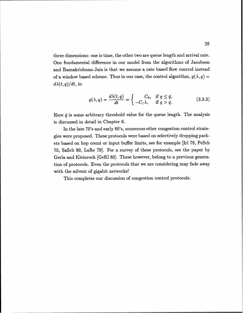
three dimensions: one is time, the other two are queue length and arrival rate.

One fundamental difference in our model from the algorithms of Jacobson

and Rarnakrishnan-Jain is that we assume a rate based flow control instead

of a window based scheme. Thus in our case, the control algorithm, g(X, q ) =

dX(t, q)/dt, is:

Here Q is some arbitrary threshold value for the queue length. The analysis

is discussed in detail in Chapter 6.

In the late 70's and early 80's, numerous other congestion control strate-

gies were proposed. These protocols were based on selectively dropping pack-

ets based on hop count or input buffer limits, see for example [Irl 78, PeSch

75, SaSch 80, LaRe 791. For a survey of these protocols, see the paper by

Gerla and Kleinrock [GeK180]. These however, belong to a previous genera-

tion of protocols. Even the protocols that we are considering may fade away

with the advent of gigabit networks!

This completes our discussion of congestion control protocols.

Chapter 3

Evaluation of Error Recovery Protocols with Independent Packet Errors

3.1. Introduction

We start discussion by limiting the degrees of freedom to the case where

(a) packet errors are independent and (b) the underlying network is a LAN

(Local Area Network). These will be relaxed in the later chapters. As men-

tioned before, we are interested in quick response times for multi-packet

message transfers. We shall evaluate the performance of the different re-

trasnsmission protocols over a local area network, characterized by low error

rates, high bandwidth and low propagation delays.

Degradation of performance could result from a number of factors. It

could be caused by flow control (for example, the outstanding window size

could be very small), or by the host to network interface, or it could be

caused by the choice of retransmission strategy in case of errors. Our focus

here is on this last issue. The principle retransmission strategies that we

consider are the blast protocol with f i l l retransmission o n error ( BFRE),

the go-back-n protocol, the selective-repeat protocol and the optimal blast

protocol that we propose. Zwaenepoel [Zwa 851, presents an analysis of

BFRE. He also presents limited simulations for the go-back-n and selective-

repeat protocols, which suggest go-back-n as the strategy of choice for local

area network environments. One of our contributions is the analytical eval-

uation of the go-back-n and selective-repeat retransmission strategies for a

multi-packet message. Our results corroborate those of Zwaenepoel: BFRE

becomes unstable much faster with respect to message size than go-back-n

or selective-repeat. However, BFRE has a very simple state machine and

makes other design issues much simpler and efficient, see for example the

network interface design of Kanakia and Cheriton [KaCh 881. It also seems

ideally suited for an environment where host processing time is a significant

amount of the total time, precisely because the amount of "work" to be done

by the host is reduced. This is the motivation for our optimal blast protocol

which performs well for both large and small message sizes.

Previous analyses of go-back-n and selective-repeat assumed low nodal

processing times, high error rates and high link delays [AnPr 86, BrMo 86,

MQR 871. The principal focus of those studies were on maximization of

channel throughput, given assumptions of packet arrival rates and distribu-

tions. While that clearly was a viable goal for some environments, it is not

the main focus for users interested in say, accessing files or making remote

procedure calls over networks, where response times determine workstation

performance. Towsley [Tow 791 had an interesting analysis of the go-back-n

retransmission strategy, deriving formulas for individual packet delays un-

der general assumptions of the distribution of packet arrivals at the sending

site. This analysis would be more suitable for the nodes in store and forward

networks.

Our study focuses on the statistics of the time to complete a multi-packet

message transfer. We address both processing and transmission times. Most

related work in this area, with the exception of [Zwa 851, ignore processing

time as a negligible component of the delay. Measurements on local networks

have shown that this delay is in fact significant.

The rest of this chapter is organized as follows. Section 3.2 presents

the model and its assumptions and the protocol definitions. Sections 3.3

and 3.4 present the analyses of go-back-n and selective-repeat respectively.

Numerical results comparing these protocols are presented in Section 3.5.

We shall see that the performance of BFRE is very sensitive to message size.

In Section 3.6, we propose and evaluate the Optimal Blast Protocol which

increases the range of operation of BFRE. Section 3.7 presents the analysis of

go- back-n under the assumption that the transmission and processing times

are generally distributed. Section 3.8 presents our conclusions and Appendix

3.A and 3.B fill in some of details omitted in Section 3.4.

3.2. Preliminaries

The Model Figure 3.1 represents a typical network interface architecture. To transmit

a packet, a station copies the data from host memory to interface memory

and then transmits it onto the network.

When a packet arrives at a station, it is first put in interface memory

from where it is copied to the host's memory. Messages are assumed to be

comprised of fixed size data packets. The time to copy a data packet between

host memory and interface memory is assumed to be a constant C. The time

to transmit a data packet is assumed to be a constant T. The corresponding

times for acknowledgment (ACK) packets are Ca and Ta respectively. Prop-

agation delays are assumed to be negligible. C and Ca are limited by the

DMA rate of the host bus. T and T a are limited by the network's speed. In

the analyses of Sections 3.3 and 3.4, we assume that there is just one send

buffer. In case of multiple send buffers, the timing diagrams used in these

analyses will change, but the method of analysis and the relative performance

of the different protocols will not. In fact, we do generalize the analysis of

go-back-n to handle arbitrary timing sequences. The focus here is on the rel-

ative performance of different retransmission schemes. We feel our analysis

should be straightforward to extend to newer and faster interfaces.

Figure 3.2 shows the timing diagram of a simple sliding window protocol.

We have assumed that the window size is large enough so that it does

not close. The horizontal axis represents time. The upper, middle and lower

network

Figure 3.1: Network Interface Architecture

lines correspond to sending station, network and receiving station activity

respectively. In this diagram, we show each packet being separately acknowl-

edged. The sender first copies a packet from its memory to its interface. This

takes C time units. The network transmission of this packet takes T time

units. The data is then copied at the receiving end taking another C time

units. Simultaneously, the sender transmits the next packet. Every packet is

separately acknowledged. Copying of the ACK packet to the interface takes

Ca time units and its network transmission takes Ta time units. Figure 3.3

shows the corresponding timing diagram of the Blast protocol. Here, the

I , T1 Tend I' -4

i C I

sender C i C Ca - - Ca - - CB - I 1

network T T Ta T T_a Ta -- - - -

receiver - - - - c Ca C Ca C Ca

Time Figure 3.2: Timing Diagram of the Sliding Window Protocol (No Errors)

T1 w Tend - - 8 : C

I

sender C j C - CB - I I I

network T T T Ta - -

receiver

*

Time Figure 3.3: Timing Diagram of the Blast Protocol (No Errors)

receiver transmits an ACK only at the end of transmission of all packets.

In both these timing diagrams, it is assumed that there is one interface

buffer for sending and one for receiving, and that the interface processes

one packet at a time. This makes it possible, for example in Figure 3.2,

for the the sender's data transmission to overlap with its processing of an

acknowledgment, i.e., data can be transmitted onto the network while an

ACK packet is being copied into host memory. However, copying of data

to the interface from the host cannot be overlapped with transmission of

the data onto the network. The actual timing diagram will depend on the

implementor's choice of signals and when they are masked off or turned on.

It would also depend on the number of send buffers provided. However,

the analysis we present in the next section would still remain valid if the

time parameters chosen were suitably modified. In fact our analysis can

be extended in a straightforward manner to the faster interfaces that are

currently being designed [SoLa 88, KaCh 881.

The next important parameter of the model relates to packet error rates.

Error rates in local networks are extremely low. If one out of every n bits are

in error due to electrical noise, the probability of a packet of size b bits failing

is 1 - (1 - l/n)'b/n + o(b/n). If data is transmitted as packets of 1K bytes

each then the probability of a data packet failing is 8K/n. The corresponding

packet failure rate for an ACK packet of say 64 bytes, is 512111. For a bit

error rate of one in 10' to one in 10'' or less, these values are extremely low.

We are not aware of any authoritative report on the actual bit error rates on

local networks. However, they seem to be sufficiently low, not to warrant any

concern for performance degradation just by themselves (as we shall see in

Section 3.5). The advent of optical fibers reduces errors to even lower rates.

However, although collisions (in case of random access protocols) are rare,

the increased use of remote file servers and other distributed applications

are likely to increase their frequency. In addition, various studies [SoLa 88,

Zwa 851 have reported significant error rates at network interfaces generally

resulting from unavailability of buffers. Indeed Zwaenepoel suggests that

packet error rates caused by interface errors are in fact somewhere in the

range of one in lo4 to one in 10' [Zwa 851. Since this dominates network er-

rors caused by random noise, we assume in our analysis that all packets have

the same probability of failing, irrespective of packet size. This probability,

which we denote by po, is an important parameter in our model. As we men-

tioned at the beginning of this chapter, we assume that these packet errors

are statistically independent, much as in [Zwa 851. We shall see that this

simplifying assumption actually helps shed some light on the performance of

these protocols. However, this restriction will be removed in Chapter 5.

3.2.3. The Protocols

The protocols we are interested in are essentially retransmission strate-

gies. We distinguish here between transmission and retransmission strate-

gies. Briefly, the time when the receiver sends an ACK determines the trans-

mission strategy (for example Blast and Sliding-Window are two different

transmission strategies). A retransmission strategy, on the other hand, de-

termines which packets are retransmitted in case of errors.

If the transmission strategy is sliding-window, the go-back-n and selec-

tive repeat retransmission strategies work as follows: when a packet success-

fully reaches the receiver, it is always ACKed if it is "in-sequence". In case of

selective-repeat, the receiver buffers out of sequence data. In both cases an

error is detected at the sender by either a timer interrupt or by a NACK from

the receiver. At this point, if the sender backs up to the first packet in error

and restarts the transmission, the strategy is referred to as go-back-n [Tan

811. If, on the other hand, the sender retransmits only that packet which is

in error, the strategy is called selective-repeat. In go-back-n, reassembling of

the message at the receiver is much simpler than in selective-repeat, but at

the potential cost of retransmission of many more packets.

The mechanisms for go-back-n and selective-repeat are similar if the

transmission strategy is Blast. For a N-packet transfer, the first N-1 packets

are transmitted unreliably (i.e., with no corresponding ACKs). The last

packet is transmitted reliably, i.e., it is retransmitted periodically until an

ACK is received. This ACK indicates the first packet in error in case of go-

back-n, and all the packets in error in case of selective-repeat. The receiver

also has a NACK capability to flag an error immediately when it is detected.

In BFRE, all the packets are retransmitted, irrespective of which packets

were in error. We have chosen to associate Blast as the transmission strategy

with it. A sliding-window version with full retransmission seems to make

less sense, because packets which have already been ACKed may then be

(unnecessarily) retransmitted.

3.3. Go-Back-N Retransmission Strategy

In the go-back-n retransmission strategy, the sender retransmits all pack-

ets from the first packet in error. The receiver does not buffer out of sequence

data. This simplifies the state machine, but at the potential cost of multiple

retransmissions of successful packets. However, as we shall see, more sophis-

ticated protocols cannot really improve on the performance of this protocol

for realistic error rates.

3.3.1. Notation We define the following symbols:

C : time to copy a data packet between host memory and interface memory

T : time to transmit a data packet onto the network

Ca : time to copy an acknowledgment (ACK) packet between host memory

and interface memory

Ta : time to transmit an ACK packet onto the network

TI : C + T, time between the initiation of two successive data transmissions

Tend : 2C + T + 2Ca + Ta, time taken (as seen by the sender) to transmit

the last packet and receive its acknowledgment.

T : The time to detect an error at the sender gs'ven that a n error has occurred.

In Appendix 3.A, we have shown that for practical error rates, the variance

of T is very small in the presence of negative acknowledgments. We thus

treat it as a constant here.

Analysis

This subsection presents the analysis of the expected time and the vari-

ance of the time to transmit N packets in the presence of errors. We assume

deterministic processing times (C, Ca) and transmission times (T, Ta) and

ignore queueing delays. We also assume that the sender can always send

(i.e., if there is a window, it never closes), an assumption justified in light of

our previous assumption of deterministic delays and no queueing.

Our analysis assumes a sliding window transmission scheme. A packet

transmission fails when either the data packet or its corresponding acknowl-

edgment is lost or is corrupted. Note that the failure of an acknowledgment

does not necessarily mean a failed packet transmission, if for instance the ac-

knowledgment for the next packet arrives before the sender times out. So this

assumption overestimates the effect of an error and gives a lower bound on

the performance of go-back-n. As stated in the previous section, we assume

that packet failures are independent of their size and are also statistically

independent. We denote the probability of packet failure by po. Given these

assumptions, the probability that a packet transmission fails is:

Now, suppose that the first failure occurs after r packets are successfully

sent. The time to send the r packets and detect the error at the sender's site

is :

Tf(r) =rTl + T , O I r 5 N - 1

where Tf indicates a failed transmission. For simplicity, we denote q = 1 - p. In go-back-n, the failure of a packet transmission marks a regeneration point

of a stochastic process because all the packets starting from this point on-

wards have to be retransmitted. The probability of a regeneration occurring

after r packets is qrp.

The last packet sequence transmitted will have no errors. We denote

the time for this transmission by T,(r), where r is the number of packets

transmitted in this last sequence.

Its probability distribution is qr .

Let the total time to successfully transmit N packets with the go-back-

n strategy be T N . If there are k regenerations (retransmission sequences),

with r; packets transmitted during the i th retransmission, then the total time

taken (denoted by T(N1k) ) is :

T(Nlk) = x ~ ~ ( r i ) + T.(N - x r,)

The above equation simplifies to

Let pk be the probability that there are k regenerations given N packets.

Since the last transmission always carries at least one packet successfully,

the number of ways in which k regenerations can occur given N packets is

) see this, note that this problem can be mapped to the problem ( N + k - l k - of finding all possible integer solutions to the equation

where X i >_ 0 for i = 1,2, - - - k and Xk+1 2 1. Now, let XL+l = Xk+l - 1,

so that X i + , >_ 0. Then the previous problem is analogous to finding all

possible integer solutions to

N+k 1 which is ( - ). Then pk is given by

The expected time to transmit N packets successfully is now easily obtained:

Now,

and

and noting that q = I - p, this becomes N : Thus E[TN] is given by

Equation 3.2 has an obvious intuitive appeal. If p = 0, E [TN] = ( N - l)Tl + Tend is the time for an error free transmission (see Figure 2.2 ). For every

failure, there is a cost of T to detect the error. The average number of errors

is the expectation of the distribution given by Equation 3.1 and is equal to

N:.

We next compute the variance of the transmission time with the go-

back-n strategy.

Now, noting that k2 = k(k - 1) + k

The first term on the right hand side can be derived in a manner similar to

the derivation of Equation 3.2, except that we need to work with the second

derivative now:

The second term is equal to N p l q , as derived before. These finally give

Equation 3.3 shows that the variance of the transmission time is proportional

to the variance of the number of regenerations. The proportionality constant,

r2, is small compared to the entire transmission time (see Appendix 3.A).

Acknowledging every packet (or at least NACKing packets in error), reduces

the time to detect an error. This is the only extra cost in go-back-n for each

error.

A more complete analysis which accounts for variable transmission and

processing times is given in Section 3.7. Assuming that TI, Tend and T are

generally distributed i.i.d (independent and identically distributed) random

variables with finite first and second moments, we find that the expected

time and the variance of TN are given by

and

v ~ T ( T N ) = (N - l )va~(Tl ) + vaT(Tend) + E[T]~N; + iVPvaT(~d) Q Q

Selective Repeat

In this section we present the analysis of the selective repeat protocol.

Several variations of this protocol have been proposed. Most assume that

packet error rates are very high. Since this is not true in the LAN envi-

ronment, we choose the following simple version. The sender transmits all

N packets in the first round. The receiver sends an acknowledgment at the

end of the round with a bit vector indicating the packets in error; these are

retransmitted in the next round. This procedure continues until all packets

have been successfully transmitted and received.

If there are k packets transmitted in a round, then the time taken is

kTl + Tohd, where TI = C + T as before, and Tohd is the overhead per round.

I - - -4 --4 .---.I Tohd Tohd Tohd

Time

Figure 3.4: Selective Repeat, N = 5

We assume in the following analysis that the the sender always gets the ACK

back after a time Tohd. This assumption is strictly not necessary, but makes

the results more intuitive and understandable. The analysis resulting from

this simplification should favor selective repeat. Our main motivation in this

section is to show that selective repeat cannot do very much better than go-

back-n for practical error rates, so we choose to favor intuitive understanding

over rigor.

To motivate the analysis, the reader is referred to Figure 3.4. We have

broken the time line, as viewed by the sender, into rounds. In each round,

all outstanding packets are transmitted. Correctly received packets are indi-

cated by a tick while those requiring retransmission are indicated by a cross.

The time line can be seen to consist of the sum of two random variables X

and Y, where X is the sum of all the TI7s and Y the sum of all the Tohd9s.

The time to complete transmission of N packets is

and therefore,

E[TN] = E[X] + E[Y]

and

var(TN) = var(X) + var(Y) + 2cov(X, Y)

where cov(X, Y) is the covariance of X and Y and is given by [Tri 821

The covariance term is not zero because the number of packet failures and

the number of rounds are related (for example, the number of errors is at

least equal to one less than the number of rounds).

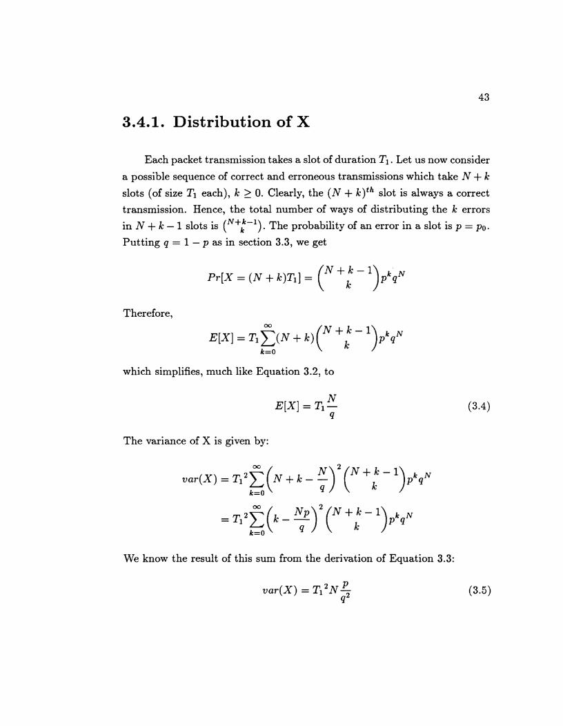
3.4.1. Distribution of X

Each packet transmission takes a slot of duration T I . Let us now consider

a possible sequence of correct and erroneous transmissions which take N + k

slots (of size Tl each), k 2 0. Clearly, the ( N + k)th slot is always a correct

transmission. Hence, the total number of ways of distributing the k errors N+k-1 in N + k - 1 slots is ( ). The probability of an error in a slot is p = po.

Putting q = 1 - p as in section 3.3, we get

Therefore,

which simplifies, much like Equation 3.2, to

The variance of X is given by:

We know the result of this sum from the derivation of Equation 3.3:

3.4.2. Distribution of Y

For every round, we have a fixed overhead Tohd. If there are R rounds

then Y = Tohd * R. Now, the distribution of R is given by

which simplifies to N

Pr[R 5 k ] = (1 - p k )

Viewed another way, since the total number of rounds is 5 k, each packet

is transmitted successfully in at most k attempts. The probability of this

event is (1 - p k ) . Since there are N packets, all of them encountering errors

independently of each other, we get Equation 3.6. The expected cumulative

overhead E[Y] is now given by

= Tohd [g k=O [I - (1 -P',"]]

For N p << 1, this last expression can be approximated by

E[Yl 2 Tohd ( 1 + C N P ~ )

= Tohd (1 + N ; )

The variance of Y is given by:

Now using the formula for summation by parts, and assuming N p << 1, we

can approximate this as follows:

2 1 [(k + 1 - (1 + $)I2 - (k - (1 + $))2] * k=O

and this finally yields

Equations 3.7 and 3.8 along with the covariance term from Appendix 3.B give the variance of the transmission time of selective repeat.

3.5. Numerical Results

This section compares the mean and variance of the transmission times

of the go-back-n, selective-repeat and the BFRE protocols. The curves for

BFRE are obtained from the analysis of [Zwa 851. The results for go-back-n

and selective-repeat are obtained from the derivations in Sections 3.3 and 3.4.

We use the measured values of C, Ca, T and Ta reported in [Zwa 851 (Table

3.1). These values are getting progressively smaller with faster networks and

interfaces, but we expect the relative times to be similar at least in the near

future.

Table 3.1: Parameter Values

Parameter

C Ca T Ta

Figure 3.5 shows the expected time to transfer N packets for the different

protocols, for N = 64 and N = 512. For N = 64, all three protocols have

almost the same expected time for a packet error rate of to (the

error range that we can expect in a local area network environment). As N

increases, BFRE starts performing poorly. Go-back-n however fares almost

as well as selective repeat even for N = 512.

An estimate of a parameter could be misleading without an estimate of

its error. We therefore plot the standard deviation of the transmission times

in Figure 3.6. The curves are for N = 64. The curve for BFRE assumes that

the receiver has the NACK capability so that the sender can detect a failed

transmission early. Go-back-n can be seen to have almost as low a standard

deviation as selective-repeat for the error range of to Selective-

repeat does better for error rates of and higher but that portion of the

curve is not significant from a practical standpoint. The key point here is that

go- back-n has a simpler state machine than selective-repeat and performs

almost as well.

Value

1.35 msec 0.17 msec 0.82 msec 0.05 msec

0

N=512 ; / go-back-n

51 / ,' . . . . . -+-.

0 .............+. :;::::::... ...; ........... +*:r.-2d----

8 " sei. rep. " N164 - B F ~ / - b a c k - n

sel. rep.

Log ( Packet Error Rate )

Figure 3.5: Mean time to transfer N packets

versus packet error rate

I go-back-n

Log ( Packet Error Rate )

Figure 3.6: Standard deviation of the time to

transfer N=64 packets versus packet error rate

Log ( Packet Error Rate )

Figure 3.7: Standard deviation of the time to

transfer N=512 packets versus packet error rate

In Figure 3.7, we have plotted the standard deviation curves for N =

512. This shows that even for large N, go-back-n is still a viable protocol.

This figure clearly demonstrates that for large messages, the BFRE protocol,

if adopted, should be decomposed into multiple BFRE7s. We address this

point in the next section in more detail. For large messages, we shall see

that adding a checkpointing mechanism to BFRE at the right places is also

a good alternative.

Optimal Blast Protocol

The Blast protocol with full retransmission on error (BFRE) is aesthet-

ically simple and seems to take full advantage of the low error rates and

high bandwidth of local area networks. However, its performance, especially

the variance of the time to transfer large messages degrades considerably as

message sizes increase. To avoid the performance penalties, without sacri-

ficing much of the simplicity of the BFRE protocol, transmission of a large

message can be decomposed into multiple BFRE's.

The number of packets in each BFRE could be fixed apriori or could be

variable, with the latter enjoying the obvious advantages:

( i) Dynamic adjustability to changes in observed network error rates.

( ii) Tuning according to each individual sender's performance objectives.

The first point is obvious, especially if the error rates fluctuate with time

(provided, of course, they can be estimated accurately). The second point

emphasizes that the optimization criteria of different communicating pairs

need not be the same. In the following discussion, we choose not to minimize

the expected time to transmit a message because it is almost equal to the

error free transmission time for practical error rates. Instead, we propose to

constrain the standard deviation of the time to transmit the packets to some

constant times the expected time to transmit the packets successfully. That

is, the standard deviation, which we interpret as the error in the estimate of

the mean, is constrained by the following equation:

Typically, we would like r to have a very small value. Equation 3.9 says that

we are less willing to accept large deviations for smaller messages than for

larger messages. Also, we want the standard deviation to be smaller than

some constant times the expected time to transmit the entire message. r

serves as an upper bound on the coefficient of variation of TM. To achieve this desired standard deviation, for an M-packet-transfer, we

propose to "checkpoint" the (blast) transmission by requiring a mandatory

ACK from the receiver after every N packets, where N is the largest value

such that Equation 3.9 is satisfied. This means that we have approximately

M / N BFRE's in series, each of N packets. We call N the optimal blast size.

Let each BFRE be of size at most N packets. Let n = M / N . Then,

ignoring the end effects of truncation and assuming that successive BFRE's

are statistically independent, we have

and

The constraint in Equation 3.9 can then be rewritten as

n v a r ( T N ) 5 T ~ E [ T ~ ] ~ = r 2 n 2 ~ [ T N 1 2 (3 .12)

Now, if the receiver NACKs on errors, [Zwa 851 shows that the variance of

the time to transmit N packets using BFRE is

where t o ( N ) represents the time to transmit N packets with no errors, p

is the probability of a BFRE failing and q = 1 - p. The expected time to

transmit the N packets is

From Equations 3.12, 3.13 and 3.14 we get

and since n = M I N , we have

The probability of a BFRE failing, p, is of course dependent upon N. It is

the probability that at least one of the N packets that are transmitted fail,

and is given by N + 1

P = ~ - ( ~ - P O ) (3 .16)

Given M , r and po, we can obtain N by solving Equations 3.15 and 3.16

iteratively to obtain the optimal blast size which satisfies Equation 3.9. Al-

ternatively, when N p << l, we have from Equation 3.16

and therefore

Figure 3.8:

M, total #packets

Figure 3.9: Optimal number of packets per sub-blast for po = lo-'.

In Figures 3.8 through 3.10, we show the optimal blast size for error

rates between and lo-*, for different message sizes, M. Both the axes

are in units of number of packets. It is interesting to see how the optimal

blast size drops rapidly with increasing p decreasing T . In Figures 3.11 and

3.12, we show a comparative performance of the optimal blast protocol and

M, total #packets

Figure 3.10: Optimal number of packets per sub-blast for po =

the normal BFRE protocol. The optimal blast protocol in these figures uses

the optimal blast size for any particular M, r and p. In Figure 3.11, we have

plotted the ratio of the expected times of the optimal blast protocol and

BFRE. This value is close to unity. However, in Figure 3.12, we see the very

sharp improvement in the standard deviation of the time, which essentially

means that we have increased the confidence in the estimate of the mean

almost for free. The reason is that the expected time is almost equal to

the error free transmission time for practical error rates, but the standard

deviation can still be large for large message sizes. We however see one

problem with the optimal blast protocol: for small M, the ratio of the two

expected times is greater than unity, especially as r gets smaller. This is

because in our optimal blast, the sender waits for an ACK of the previous

packet group before it starts transmitting the next packet group, causing

the pipeline to empty out and fill up again for each sub-blast. The delay

resulting from this dominates over the expected time of a simple BFRE for

smaller message sizes because the probability of a retransmission is extremely

low. Smaller values of r increase the number of sub-blasts (see Figure 3.10)

exacerbating the problem. However, as M increases, one of the properties of

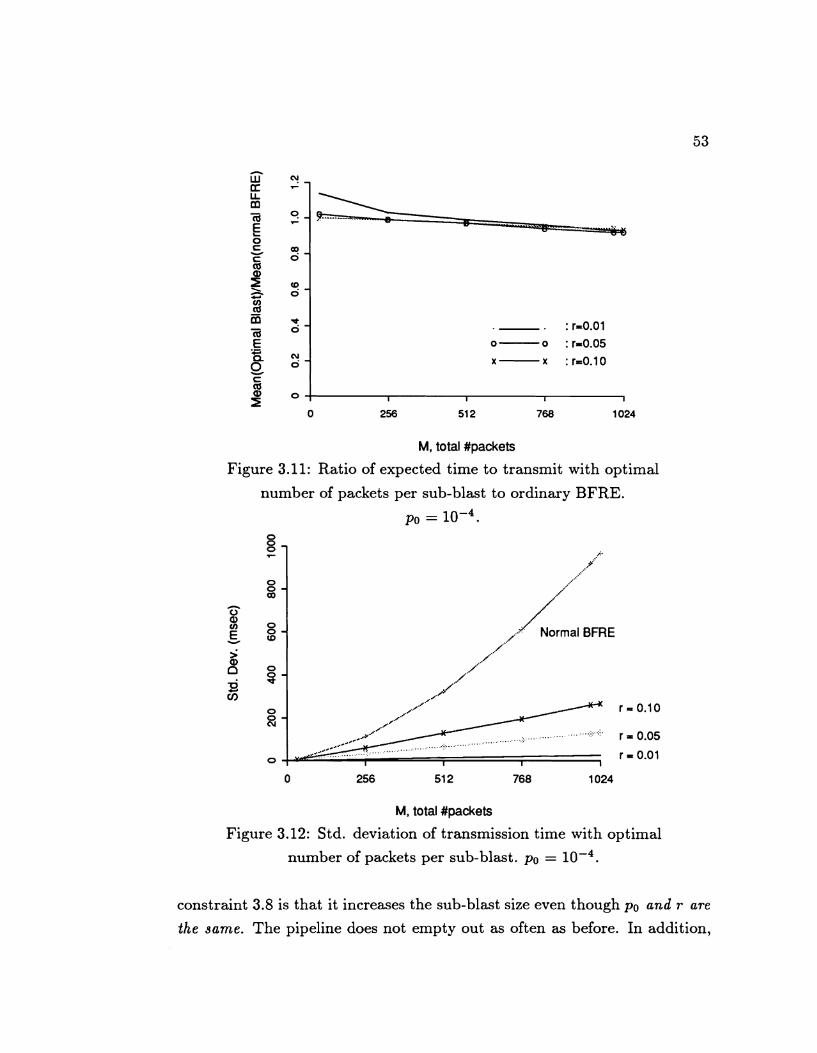
. - . : r=0.01 0- o : r=0.05 x-x :r=0.10

M, total #packets

Figure 3.11: Ratio of expected time to transmit with optimal

number of packets per sub-blast to ordinary BFRE.

= lo-*.

M, total #packets

Figure 3.12: Std. deviation of transmission time with optimal

number of packets per sub-blast. po =

constraint 3.8 is that it increases the sub-blast size even though po and r are

the same. The pipeline does not empty out as often as before. In addition,

the probability of a retransmission increases for the simple BFRE. These

factors pull the ratio of the expected times below unity as the total number

of packets, M, increases. The standard deviation to the transmission time

improves for all M, though it is more pronounced for large M.

To prevent the degradation in the expected transmission time for small

M, we propose the following modification to the protocol:

( i) The sender determines the optimal blast size, N, for the given message.

( ii) It then transmits packets 1 through N - 1 in the current BFRE

without requesting an ACK from the receiver.

( iii) It transmits packet N with the REQUEST-FOR-ACK bit set.

( iv) Without waiting for the ACK, it continues with the next blast using

steps (ii) and (iii).

( v) The receiver ACKs the packets which have their REQUEST-FOR-

ACK bit set, provided it has received all the packets with sequence

numbers greater than the previously ACKed packet and less than the

current one. It can also NACK packets in error. Dropped packets

however will have to be detected by the sender's timeout mechanism.

( vi) In case of an error (either a NACK or a timeout), the sender re-

transmits the whole "window" of outstanding BFRE's not yet ACKed.

This leads to a go-back-n retransmission across sub-blasts, although each

smaller sub-blast is still fully retransmitted!

We note that the sender does not have to negotiate the sub-blast size

with the receiver in advance. In a window based flow control scheme, there

has to be space for the packet when it arrives at the receiver, but flow con-

trol and error control are orthogonal functions here. One bit in the packet

could serve as REQUEST-FOR-ACK/ NO-ACK, and could be set whenever

the sender wants an ACK. Thus the size of a sub-blast could change with

time even between the same communicating pairs. This could happen, for

instance, if the sender's effective window size drops because it senses conges-

tion. [Jai 861 and [Jac 881 claim that packet errors are a good indicator of

congestion, and their congestion control protocol shrinks the effective winz

dow size to deal with it . The window is slowfy increased after that. Their

scheme fits in harmoniously with the sender's choosing the optimal blast

size independent of the receiver. All that the sender has to do is to set the

sub-blast size as min {N, congestion-window, flow-window ) , where N is the

optimal blast size from Equations 3.15 and 3.18.

3.7. Generalized Analysis of Go-back-n

We now generalize the go-back-n results by removing the deterministic

time constraints under which the results were obtained in Section 3. We begin

with some notation and definitions. Denote the time from the beginning of

the transmission of packet i to the beginning of the transmission of packet

i + 1 by the random variable Xi, if the packet transmission was successful,

i.e., both the data packet and its ACK were successful. This corresponds

to TI in Section 3.3. The time corresponding to Tend is denoted as Xend.

Thus Xend is a random variable denoting the time from the beginning of

the transmission of the last packet until its ACK is received, given that the

transmission is successful. Similarly let T, be the time to detect the ith error

if one occurs. It is easy to see that the time to transmit N packets given

that k regenerations have occurred is

We assume that the Xi's are independent and identically distributed random

variables with mean E [XI and second moment E [X2]. Also let their common

Laplace transform be X(s). Likewise we assume that E[Xend], E[x,,~~] and

Xend(s) are the mean, second moment and Laplace transform of Xend, and

E [TI, E [r2] and ~ ( s ) are the mean, second moment and Laplace transform of

T respectively (of course, we are assuming the T, to be i.i.d. random variables

too). Then the Laplace transform of T ( N ) which we denote by T ( s ) is given

by

Taking the natural logarithms of both sides of Equation 3.17, we get

Notice that E[X] = -&x(s) I and E[X2] = $x(s) I , and similarly a = l a = l

for the other random variables. Thus differentiating the left hand side of

Equation 3.18, once and putting s = 0 gives E[TN] and differentiating it

twice and evaluating it at s = 0 yields var(TN). The resultant equations

are:

E[TN] = (N - l)E[X] + E[Xend] + E[r]NP- (3.19) Q

and

For the deterministic case in Section 3, E[X] = TI, E[Xend] = Tend,

E[T] = T and var(X) = var(Xend) = var(r) = 0. As one would expect,

the result is the same as given by Equations 3.2 and 3.3. Equations 3.19

and 3.20 are independent of the actual distribution of the Xi's and ri's, but

depends only on their mean and variance. It is clear that the variance of

the time to successfully transmit N packets will increase linearly with the

variance of the protocol processing and transmission times and the time to

detect errors. Also, Equations 3.19 and 3.20 are more general in the sense

that they factor in various unaccounted for "random delays."

We do not have any red-life data on the variance of packet processing

times and transmission times. In real implementations, there is likely to be a

variation in packet processing times by the two stations. The variance of the

transmission times could also be caused by network load, which, although

usually low, can occasionally be quite high [Gus 871. It is our surmise that

packet processing and transmission times will be normally distributed about

their mean, but this needs empirical verification. Equation 3.20 is valid only

if the random variables X i , Xend and the ri's are independent of each other.

It should apply to protocols implemented at the transport level or below,

where correlations among consecutive packet transmission times are likely

to be weak. The results of this section provide a means of isolating the

communication of a pair of nodes from all other traffic. To some extent we

have an expression for the mean and the variance of the delay for a bulk data

transfer under a multiple-sender/multiple-receiver assumption. The results

also apply to multiple hop transmissions, provided that windows never close

at intermediate stations. The main problem that remains is to determine

the mean and the variance of the Xi's and Xend. The latter is likely to be

more important as the number of hops increase and/or load from the other

connections increase.

3.8. Summary and Conclusions

We presented analytical results for the expectation and the variance

of transmission times for different retransmission strategies over local area

networks. For small messages (i.e., small number of packets per message),

BFRE, go-back-n and selective-repeat, all perform well. However, as the

message size increases, BFRE shows larger mean and variance than go-back-

n while the latter does almost as well as selective repeat. These conclusions

are based on an estimate of the packet error rate between and

More reliable network interfaces will likely reduce error rates on local area

networks. Under such conditions, BFRE will perform almost as well as the

others, and given its simplicity, will be a more attractive protocol. For error

rates which we observe today, go-back-n and the optimal blast protocol will

be more viable alternatives since any protocol has to deal with a wide range

of message sizes.

We also extended the analysis of go-back-n to handle the second order

effects of variable processing and transmission times. We assumed a general

distribution of delays, instead of a deterministic one and showed how they

affect the expected time and the variance of the transmission time of large

messages. Possible applications of this model are datagram oriented trans-

port protocols with associated protocol processing overhead, variable delays

due to multiple connections, and variable transmission times due to network

load. We found that for go-back-n the variance of a message transmission

time increases linearly with the variance of individual packet transmissions

in addition to that contributed by erroneous transmissions.

This study needs to be extended in many directions. We incorporate

windows into our analysis in the next chapter. The effect of buffer non-

availability at intermediate nodes (and the resultant correlated packet losses)

is studied in Chapter 5. The effect of varying the transmission rates so as to

reduce these packet losses is discussed in Chapter 6 .

Chapter 4

Go-back-n with Windows

4.1. Introduction

In this chapter, we incorporate windows into the analysis of the go-back-

n protocol. Previous studies have either been on flow control strategy or error

control strategy in isolation [Mor 88, ToWo791. The complexity of analyses

has usually precluded a simultaneous study of both. Our main result in this

chapter is that under certain circumstances, sliding window and go-back-n

are quasi-independent in that they could be studied independently of each

other and the results put back together in a straightforward manner. Thus,

the window flow control protocol can be analyzed with models of varying

complexity and then combined with the term representing the cost of errors.

This quasi-independence property is only an approximation, however.

It is a good one for go-back-n but not for selective repeat. The rest of this

chapter therefore, concentrates on go-back-n only.

4.2. Petri Net Models

Our goal is to show that sliding window flow control and go-back-n error

control are quasi-independent . In the previous chapter, we had seen that this

result was true when the window did not close, i.e.,

RdytoSend

Credits Avail

RecvAck (311)

AckAvail

Figure 4.1: Simple sliding window flow control: Model I

where is the expected time to transmit N packets in the presence of

errors using go-back-n, EITnoErrors,N] is the time it would take to transmit

N packets in an error free channel and ( N p l q ) ~ is the extra cost due to

errors, using go-back-n. We generalize this result here to the case when the

window may close, even wi th high probability.

Figure 4.1 shows a Generalized Stochastic Petri Net (GSPN) model

[MBC 841 of a simple sliding window flow control protocol ignoring all errors

and retransmissions. If the place RdytoSend has a token, the sender can send

a packet provided the place CreditsAvail has a token too. The mean time

to send a packet is l / X 1 . When a packet is sent, one token from each of

the above two places is removed; one is added to the place W a i t A c k where

the sender waits for an acknowledgment. Another is added to the place

CreditsUsed which is subsequently used by the receiver of the data. The

transition RecvData can fire when the receiver has a token in Rdy toRecv and

a token is available in CreditsUsed. Upon receipt of the data, the receiver

sends an acknowledgment packet which takes a mean time of 1 /X4 . Notice

RdytoSend CreditsAvail

Figure 4.2: Sliding window flow control with go-back-n retransmission: Model I1

that there are no errors in this model. For future reference, we shall call this

Model I.

In Figure 4.2 we have the GSPN model of the same sliding window

protocol but this time it includes the go-back-n retransmission strategy. In

case of an error, all packets from the first packet in error are retransmitted. In

the petri-net model, we suppress transmission of those packets which follow

the erroneous one by using an inhibit arc from the failed W a i t place into the

t ransmi t transition. In a real implementation, these packets would actually

have been transmitted (and then retransmitted). The inhibit arc, therfore,

is an approximation because we are ignoring some of the additional loading

effects at the receiver. The infrequency of these events should make this

approximation reasonable.

A successful packet follows the same path as in Model I. In case of an

error however, a token is deposited in the place fai ledwait . This inhibits

further transmission at the sender. After a timeout interval of T , the token

in restored to the RdytoSend place and normal transmission begins.

A packet error could occur at different points in transit. Let the aggre-

gate probability of error (of the packet or its acknowledgement) be p. In our

numerical examples later, we assume that both data and ACK packets have

the same probability of failure, pol so that p = 1 - (1 -

4.3. Analysis

4.3.1. Analysis of Model I

To study the effect of window size on throughput and round trip time of

packets, we assume that the number of packets to be sent, N, is at least equal

to the window size W, see Figure 4.1. This ensures that the sender always

has a packet to send, and its transmission is delayed only if the window

closes. Let x be the average number of tokens in the place WaitAcL Let p

= Pr[CreditsAvail is not empty], which is the probability that the window is

not closed. Then the throughput into the box marked with dashed lines is

Let ZI be the average time spent by a token in the box. By Little's law,

we have ZI = N / A ~ ~ , which implies that the expected number of packets

initiated by the sender per round-trip time is ZIAlp. The expected time to

transmit N packets and receive the ACK for the last one, EITN,noErrors]I,

is given by

Since N and p can be computed using a Petri Net analyzer and ?ZI can be

computed from x, E [TN,noErrora] I is easily obtained.

As before, let p be the aggregate probability of failure of a packet or its

acknowledgment, and let q = 1 - p. It was shown in Chapter 3 that, if the

windows never closed then

where Nplq is the expected number of errors in go-back-n and T is the

expected cost per error. This result holds even for generally distributed

processing and transmitted times. We shall show that Equation 4.3 holds

approximately even when the window m a y close. We also present conditions

under which this relation will be exact. Note that EITN,noErrors]I is com-

puted from an error free model. The significance of this result is that we can

actually analyze sliding window flow control and go-back-n error control as

two simplified separate models and put the results back together in a simple

way.

4.3.2. Analysis of Model I1

In this sub-section, we present the analysis of E[TN,,*,] using the more

detailed model in Figure 4.2. Let

Atran,= effective throughput through transition transmit ,

A ail = throughput through transition failure,

Asuc = throughput through transition success, and

r = Pr[ token in failed W a i t 1. Then, applying Little's Law to failed Wai t , we get A ail = TIT, since T is

the expected time spent in the fai ledwait place. Now, noting that Afair =

phtrans, we have

Asuc = ~ A t r a n s = (qIP)Afail,

which simplifies to

The average cycle time of a token in the successful path is obtained by

applying Little's Law to the box around the place Success W a i t :

- - N(Success W a i t ) RII =

A S U C

The expected time to transmit N packets is then given by

4.3.3. Comparison of the two methods

In Tables 4.1 through 4.6, we present the time to transmit 64 packets

as calculated by the two models. We vary the parameters p, T and W. We

assigned measured values of X I , X2, X3 and X4 as reported in [Zwa 851. Thus,

XI-' = time to copy a data packet from the sending host's memory onto the

wire = 2.17 msec

~ 2 - I = time to copy an acknowledgment packet from the wire into the

sending host's memory = 0.17 msec

X3-l = time to copy the data packet from the wire into the receiving host's

memory = 1.35 msec and

X4-I = time to copy an acknowledgment packet from the receiving host onto

the wire = 0.22 msec

The time to complete an N-packet transmission is obtained by first solv-

ing the two GSPN models and then using their outputs as inputs to Equa-

tions 4.2, 4.3, 4.4 and 4.5. It can be readily seen that the time predicted by

extrapolating Model I (in accordance with Equation 4.3) is remarkably close

to that obtained by solving Model I1 (cf. columns 4 and 6 in Tables 4.1 -

4.6). This is in spite of the fact that the probability of the window closing

or the probability of being in the failedwait state are not insignificant (see

columns 2 and 5). We also vary po from to and T from 10 to 1000

to show that this assumption is valid for a wide range of parameter values.

Let us now consider conditions under which the two models would be

equal. Comparing Model I and Model 11, we see from Equations 4.1, 4.2, 4.3

and 4.5, that the two models yield (asymptotically) identical results if

1 r p 1 -+ -= - A1 q As,,

Table 4.1: N=64, p0=W2, 2=10

Model I

Table 4.2: N=64, ~ ~ = 1 0 - ~ , ~ 1 0 0

Model II

E [ T N I I + $ ~

264.9 196.5 168.3 158.9 157.2

' w 1 2 4 8

16

P m i ~ e d ~ a i t = ~ ]

0.95 1 0.933 0.922 0.917 0.9 16

Model I

Table 4.3: ~ = 6 4 , po=10-~, 2=1m

E [TNIII

267.7 198.6 170.1 160.9 159.5

Model 11

~ [ W ~ I I

0.4450 0.2337 0.0863 0.0172 0.0009

NP E [ T N I I + - ~

381.9 313.5 285.3 275.8 274.2

P LfaiZedWait=Ol

0.6607 0.585 1 0.5420 0.5249 0.5217

W

1 2 4 8

16

Model I

E[TNII

25 1.9 183.5 155.3 145.9 144.2

E [TNIII

384.7 315.5 287.0 277.8 276.4

Model 11

P [W=OII

0.4450 0.2337 0.0863 0.0172 0.0009

P fiiledWait=O]

0.163 0.123 0.105 0.099 0.098

w 1 2 4 8

16

E[TNII

251.9 183.5 155.3 145.9 144.2

E [ T ~ I ~ ~

1554.2 1485.0 1456.5 1447.3 1445.9

P [W*II

0.4450 0.2337 0.0863 0.0172 0.0009

E [TNII

25 1.9 183.5 155.3 145.9 144.2

E [ T N I ~ + @ - ~

1551.4 1483.0 1454.8 1445.3 1443.7

Table 4.4: ~ = 6 4 , p0=10-~, ~=1m

Model I

Table 4.5: ~ = 6 4 , po=104, 2=1m

w 1 2 4 8

16

Model 11

P vailedWait=Ol

0.661 0.585 0.542 0.524 0.520

Model I

Table 4.6: N=64, po=10-5, ~=1000

P [W*II

0.4450 0.2337 0.0863 0.0172 0.0009

E [TN][[

380.3 311.8 283.6 274.2 272.6

Model 11 NP E[TNII+-T

264.7 196.3 168.1 158.7 157.0

P miLedWait=O]

0.95 1 0.934 0.922 0.9 16 0.915

w 1 2 4 8

16

Model I

E[TNII

251.9 183.5 155.3 145.9 144.2

E [TNIII

264.7 196.3 168.1 158.7 157.0

Model 11

w 1 2 4 8

16

E[TNII+$T

380.1 311.7 283.5 274.1 272.4

P[W*lr

0.4450 0.2337 0.0863 0.0172 0.0009

PfiiledWait=O]

0.994 0.992 0.99 1 0.99 1 0.990

E[TN]I

25 1.9 183.5 155.3 145.9 144.2

E[TNIlI

253.2 184.8 156.6 147.1 145.5

P[W*II

0.4450 0.2337 0.0863 0.0172 0.0009

E[TNII

251.9 183.5 155.3 145.9 144.2

E [ T N I I + ~ ~

253.2 184.8 156.6 147.1 145.5

For convenience, let us denote h = ~ p l q . Then for the previous condition to

hold, we require that 1 h

- + h = - , Alp r

Now, if the expected useful time spent per packet is t good and the wasted

time is tbad, then from Model I and our quasi-independence hypothesis we 1 have tgood = and tbad = r p / q = h. Equation 4.6 says that the expected

times derived from the two models will be equivalent if

-

r = ood I + + bad

Pr Failed Wait = 11 = t b a d

t g o o d + t b a d

This would, by itself, make perfect sense i f tgood was somehow obtained from

Model II. We are, however, calculating t g o o d = & from Model I and r from

Model II. The two models will be close if the probability that the window is

open given that we are not in the midst of handling an error in the second

model, is close to p, the probability that the window is open in the first

model. The results from the petri-net analysis suggest that this is so.

4.4. Conclusions

In this chapter, we analyzed the go-back-n protocol in conjunction with

sliding-window flow control. The analysis assumed that packet errors were

independent of each other.

We discovered that go-back-n and sliding-window flow control are quasi-

independent in that the total expected time to transmit an N-packet message

is approximately equal to the sum of the two separate results obtained by

modeling each of them independent ly of t h e other.

A similar straightforward result does n o t exist for selective repeat, how-

ever. This is because the cost per error in selective repeat is dependent on

the window size: if the window is always open for example, the cost of an

error is just the time spent in transmitting the erroneous packet; if the win-

dow were to close on the other hand, the cost would depend on which packet

in the current window failed and what t h e value of the window size was.

The difficulty is not in being able to analyze this protocol with windows (we

shall do it in Chapter 5), the problem is in obtaining a simple approximation

similar to that of go-back-n (corresponding to Equation 4.3). That still is an

open problem.

Chapter 5

Analysis of Error Control Protocols with Congestion- Dependent Errors

Introduction

In this chapter, we investigate the performance of go-back-n and

selective-repeat error control protocols and their ability to recover from con-

gestion loss. The performance measure of interest once again is the expected

time and the standard deviation of the time to transmit a large message,

consisting of N packets.

We first develop a framework to evaluate the two retransmission strate-

gies in presence of windows when packet errors are congestion-dependent.

As we noted in Chapter 1, earlier work on retransmission strategies [MLS 89, ToWo 79, Zwa 851, have assumed the independence of errors. If the cause

of packet errors is random noise in the communications channel, then this

is a reasonable assumption. However, in most networks, such random errors

are extremely infrequent. A more common occurrence is packet losses at

intermediate nodes due to lack of availability of buffers. When this happens,

the premise of independent packet errors is no longer valid. In fact, it is

more likely for a failure to occur when one has already occurred than when

none has occurred. In our study, we assume first an abstract error model

which can be used to represent any network error and then a more concrete

one for a simplified system. We then compare the two retransmission strate-

gies for different congestion models in the presence of window flow control.

We then are able to determine when an increase in window size can cause a

sharp degradation in performance, and how the two retransmission strategies

perform in such situations.

The rest of this chapter is organized as follows. Section 5.2 presents the

two congestion models. In Section 5.3, we discuss the go-back-n protocol-

model (with sliding window) and its analysis. Section 5.4 presents the same

for selective repeat. Section 5.5 compares the two retransmission strategies

with numerical examples and finally, we present our conclusions in Section

5.6.

The Model

We assume that the transmission time of a packet at the sender is expo-

nentially distributed with mean l / X 1 . At the lower levels of protocol stack

that we are interested in, the coefficient of variation of XI is likely to be less

than one. Our analysis is therefore only an approximation of real behavior.

(However, since the mean of a sum of random variables is equal to the sum

of their means, irrespective of their distribution, we expect our analysis to

be rather accurate, at least with respect to the mean time to transmit the

message).

The performance measures of interest are the statistics of the time to

transmit a large multi-packet message consisting of N packets. The sender

has a window of size w. This is the upper limit on the number of packets that

it is allowed to transmit without waiting for an acknowledgment. The sliding

window protocol, in conjunction with the go-back-n and selective-repeat re-

transmission strategies, works as follows. When a packet successfully reaches

a receiver, it is always ACKed if it is 'in-sequence'. An error is detected at

the sender by either a timer interrupt or by a NACK from the receiver. At

this point, if the sender backs up to the first packet in error and restarts the

transmission, the strategy is referred to as go-back-n [Tan 811. If, on the

other hand, the sender retransmits only that packet which is in error, the

strategy is called selective-repeat . The state machine of go-back-n is simpler

than selective repeat. Also, the selective repeat protocol may require a large

receive buffer to cache packets which are received correctly, but out of order.

Go-back-n on the other hand, can operate with one receive buffer only. So,

it is of interest to engineers and researchers to see if one can get away with

this simple strategy.

In this chapter, we address congestion-dependent packet errors, i.e., the

errors are caused by congestion in the communication channel. We develop

two models for congestion-dependent errors, an abstract model and a concrete

model. The abstract model represents any arbitrary network by a set of pa-

rameters. Careful choice of parameter values can yield useful insights on the

relative performance of the two error control protocols. The concrete model

is a first step towards a more detailed analysis of the innards of congestion.

We have so far been successful in analyzing only a single node system. In

the remainder of this section, we first discuss the abstract model and then

the concrete model.

Abstract congestion model

We assume that if the current 'congestion state' of the system is a, then

p(a) is the probability that a packet transmitted n o w will ultimately fail.

We explicitly encode the information pertaining to the current transmission

activity in a , much like in [BPU 881. The details of the background network

traffic and resource availability (or rather, un-availability) are however en-

coded by implici t parameters. Thus, for the selective repeat retransmission

strategy, we assume p(a) = p(j, k), where j is the number of outstanding

ACKs and k is the number of failures that have already taken place but

not yet recovered from. For go-back-n on the other hand, all failures after

the first one and before its detection are irrelevant. We therefore ignore the

k-component and assume p(a) = p(j), where j is the number of packets with

outstanding ACKs.

Let wmaz > w, where w is any window size that we consider. Since

p(j, k) increases monotonically with both j and k, we may approximate it

with an n-degree polynomial as follows: The j outstanding ACKs and k

undetected failures could take away a maximum of j + k buffers. In addition,

k itself indicates the level of 'badness' of the congestion. Thus we may write

where po is the intrinsic failure rate of the network and the other terms are

due to congestion. Note that the a i s and b:s are the implicit parameters

representing resource un-availability due to congestion. If we increase the

degree n in Equation 5.1, we can approximate any smooth curve more accu-

rately. One possibility is to experimentally determine the curve for p(j, k) by

generating error statistics of a specific network. While that is a worthwhile

study (and is work in progress), we can get important insights into the rel-

ative performance of go-back-n and selective-repeat by a careful exploration

of the parameter space represented by the a:s and b:s in Equation 5.1.

The constants a, and bi are such that 0 5 p(j, k) 5 1, i.e.

Concrete congestion model

Consider a single queue with a finite capacity, K. Let us assume that

this system is fed by a 'background' stream of packets with exponentially dis-

tributed inter-arrival times and a 'foreground' traffic, which is our message of

interest. Let us further assume that the service times are exponentially dis-

tributed. Then, with respect to the background traffic, this is an M/M/l/K

queueing system. Let the background traffic intensity be pb. Now consider

our designated message which arrives at this queue. Suppose that the packets

of this message are spaced tl time units apart. A proper congestion control

algorithm will at tempt to make t 1 deterministic. (This reduces 'burstiness'

and attempts to decrease buffer overruns). The question that interests us

is: what are the relative probabilities of packet overflow for the sequence of

packets of this message? (I.e., if there is a correlation, then what is it?).

The remainder of this section attempts to answer this question. First

some definitions.

Let pk(m) = Pr {k customers in queue, including the one in service,

when the mth packet of the message comes in ). Since our message arrives at a random point in time, the first packet sees the

equilibrium probability distribution for buffer occupancy given a particular

pa. This distribution is given by [Kle 751:

Clearly, the probability of loss for the first packet due to the queue being full

is pK(l). Now, if the retransmission strategy is selective repeat, we modify

the probability distribution {pk} just after the packet arrives as follows:

Essentially, this shifts the probability space one step to the right. We are

then interested in the probability distribution when the next packet of this

'foreground' message arrives, t l time units later. This can be obtained by

solving the Chapman-Kolmogorov equation for the Markov process (see [Kle

751 ) : dP/dt = P Q , where P is the probability distribution matrix, {pk},

and Q is the transition rate matrix of the queue and t is time. In our study,

we used the Uniformization technique [Jens 531, to solve for P after a time tl

given the current P as obtained by Equation 5.3. This method is summarized

Let q i j denote the ith row and jth column entry of the matrix Q. Let

q >= maxilqii 1. Set Q* = Q / q + I . Then

where

n(i) = 7r(i - I)&*, n(0) = P(0). (5.5)

We solve Equation 5.4 for t = t l with P(0) given by Equation 5.3. This gives the buffer occupancy probabilities just before the arrival of the

next packet of our designated message, from where we get the buffer over-

flow probability, p ~ . Repeated application of Equations 5.3 and 5.4 yield

the probability of overflow of the subsequent packets. The solution process

requires the computation of an infinite sum (see Equation 5.4). However, we

found that we could easily truncate this sum because its tail goes to zero

very quickly.

For go-back-n retransmission strategy, the algorithm given by Equation

5.3 is inappropriate. This is because a packet failure is relevant only if the

previous packets have been successful. Thus, if packet m arrives at time t-,

then the distribution that is of interest at time t+ is the one that will yeild

the probability of loss for packet m + 1. The probabilities computed at t+ should be conditioned on the fact that packet m succeeded. The algorithm

for modifying pk(-) is therefore

Repeated application of Equations 5.6 and 5.4 give the probability of overflow

of consecutive packets when using go-back-n.

J Figure 5.1: Probability of error in packet j for go-back-n

and selective repeat pa = 0.1 and 0.5, tl = 1.0.

In Figure 5.1, we plot some representative curves of correlated over-

flow probabilities for go-back-n and selective-repeat. Note that the selective-

repeat curves are above the go-back-n curves. This is however, n o t a disad-

vantage for selective repeat. The curve only says that the probability of a

packet loss given that there were no previous losses is lower than that with-

out any such conditioning. This is only to be expected because a packet that

is transmitted after a previous one has been lost suffers a higher probability

of loss. As long as that probability is less than one, however, the packet

still has a chance to make it to the destination. In go-back-n, this limited

chance is completely ignored. However, as we shall see later, it turns out

that the probability of loss represented by the curves in Figure 5.1 (with

or without the conditioning) are considerably high in that they degrade the

performance substantially for both go-back-n and selective-repeat. The er-

ror curve for selective repeat, which represents a limited chance of getting

through once congestion has set in, has therefore very little performance in-

centive as opposed to, say, a larger value of tl which pulls down the error

curve (this is better conges t ion control). In this case however, go-back-n will

perform almost as well as selective repeat, thus making it a viable protocol.

It is then to be preferred over selective repeat if only on grounds of simplicity.

5.3. go-back-n protocol model

In this section, we present the protocol model for go-back-n. Simultane-

ously, we incorporate the congestion models that were presented in Section

5.2. Our goal is to derive the expected time to transmit an N-packet message

using the go-back-n protocol with sliding window. To this end, a Continuous

Time Markov Process is used to chart the progress of the message transmis-

sion. The state of the system consists of a pair of tuples (i, j) where i is the

number of packets that will n o t require retransmission and j is the number

of these i packets whose acknowledgments are still outs tanding . Clearly j 5 i and also j < w, if the window size is w. In addition, we also introduce states

f i corresponding to the states where an error has occurred after i packets

have been successfully transmitted (see Figure 5.2).

Figure 5.2: go-back-n with congestion-dependent errors and windows.

The sender transmits with a mean rate A, and the acknowledgments

return with a mean rate p. Our hypothesis is that a packet fails with prob-

ability p(j) in state (i, j), where j represents the level of congestion. The

p(j), j 5 w are obtained from the congestion models of the previous section.

Figure 5.2 shows the state transition diagram of the ensuing Markov

Process. The initial state is (0,O). When a packet is transmitted, there can

be two possible next states. If the transmission is going to be successful (ul-

timately), we designate the next state as (1 ,I). Else, the packet transmission

will fail and the next state is fo. The rate into (1,l) is Xq(0) and that into

fo is Xp(0). Once a packet fails, we assume that it is detected after a mean

time T. Therefore, in Figure 5.2, we denote the rate from fo to (0,O) by T - I

which we denote by y. The rest of the arcs in the figure follow a similar

argument. Note that for all j , a failure arc from (i, j) is into f i and the

recovery arc from f i is only into (i, 0). This is a property of the go-back-n

protocol: all the packets which are transmitted before a failure are repre-

sented by i. By the time the sender detects the failure of packet i + 1 and

acts upon it, the outstanding acknowledgments of all packets upto packet i

must have returned to the sender for it to consider packet i + 1 as the first

failure and this then becomes the point of a new retransmission. Note that

our model does not capture the congestion caused by those packets which

were transmitted after a failed transmission but before its recovery. It is not

difficult to add this information but we have not done so in this study for

two reasons. First, if errors are caused by congestion, the timers should be

relatively large so as to minimize the effects of congestion. This is in con-

trast to the independent-packet-error case where a timer tuned close to the

roundtip delay is most desirable (see Equation 3.3, Chapter 3 for the per-

formance implication of the timer). Second, the complexity of the solution

process increases considerably. It may however, yield some insight into how

long the timer value should be set so as to minimize the congestion effects

of the previous packets. We shall explore this avenue in the near future.

Analysis

We next consider the transient analysis of the Markov Process of Figure

5.2. We set (0,O) as the initial state and (N,O) as the final state. We are

interested in E[TN], the time to complete an N-packet transmission. How-

ever, E[TN] is just expected time to absorption into (N,O) for this Markov

Process. To compute the expected time to absorption, we use the algorithm

in [BRT 881. Let q represent the vector of times spent in each of the states

before absorption. Let Q be the transition rate matrix obtained from the

original transition rate matrix by deleting the rows and columns involving

the absorbing states. Finally, let P(0) be the initial probability distribution

of the non-absorbing states. Then the mean time spent in each state before

absorption can be computed by solving for 77 [see BRT 881 in

The expected time to absorption is then given by

where qi,j are the individual components of 7.

The solution of Equation 5.7 is especially simple for the Markov Process

of Figure 5.2. For the states (0,O) and fo, we have

For other states (i, j ) , we get

where 1, if C = true; 0, otherwise.

Equations 5.8 and 5.9 are like 'flow equations', where we equate all the 'flows'

into state (i, j ) with all the 'flows' out of (i, j).

It turns out that for all states (i, j), j > 0 in level 2 , we have all the values

needed to compute qi,j, if we index through j from its highest possible value

in state i downwards. Once these values are available, Vi,o and 77 ji are given

in terms of each other and the other known values. This is a considerable

simplification over using a general Gaussian elimination algorithm to solve

Equation 5.7.

In Appendix 5.A, we present a method for determining the variance

of the time to absorption. The expected time to absorption falls out of

that analysis as a 'byproduct'. This helped us cross-check the numbers we

obtained by solving Equation 5.7.

The solution to Equations 5.8 and 5.9 corroborates our previous results.

For p ( j ) = p Vj, we get q f j = r p l q Vi. And if w > i, i.e. if the window does

not close at the ith level,

So the expected time to transmit N packets is

which is also a known result [MLS 891. We can also use the Markov process to

corroborate and somewhat strengthen our previous results for independent

packet error for go-back-n with windows. In fact, it can be shown that

E[TN, gbn] = E[TN, noErrors] + O(P)

5.4. Selective repeat protocol analysis

In the Selective Repeat Protocol, the sender retransmits only those pack-

ets which are in error. We represent the state of a given transmission by the

triplet (i, j, k) where i is the number of packets which have been successfully

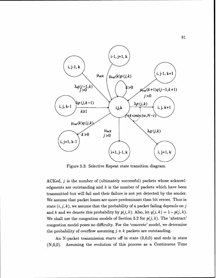
Figure 5.3: Selective Repeat st ate transition diagram.

ACKed, j is the number of (ultimately successful) packets whose acknowl-

edgments are outstanding and k is the number of packets which have been

transmitted but will fail and their failure is not yet detected by the sender.

We assume that packet losses are more predominant than bit errors. Thus in

state (i, j, k), we assume that the probability of a packet failing depends on j

and k and we denote this probability by p(j, k). Also, let q( j , k) = 1 - p(j, k).

We shall use the congestion models of Section 5.2 for p(j, k). The 'abstract'

congestion model poses no difficulty. For the 'concrete' model, we determine

the probability of overflow assuming j + k packets are outstanding.

An N-packet transmission starts off in state (0,0,0) and ends in state

(N,O,O). Assuming the evolution of this process as a Continuous Time

Markov Process, we get the state transition diagram of Figure 5.3. To model

a window of size w, we have the constraint j + k 5 w for all states (i, j, k).

If a new packet is transmitted from (i, j, k) (allowed only if j + k < w ), the

new state could be either (i, j + 1, k) or (i, j, k + 1) depending on whether

or not this transmission will ultimately be successful. The corresponding

rates are Xq(j, k) and Xp(j, k) respectively. If an acknowledgment comes

back (with rate pack) in state (i, j, k), the new state is (i + 1, j - 1, k). If a

failure is detected and the packet is successfully transmitted, the new state

is (i, j + 1, k - 1). We assume that the mean rate at which a packet error is

detected in state (i, j, k) is given by pret(k). This completes all the states to

which a transition may occur from state (i, j, k). The states from which one

may enter state (i, j, k) are shown in Figure 5.3 as a mirror image of the exit

arcs. In the subsequent discussion, we drop the subscript ack from pack.

One interesting property of the Markov process in Figure 5.3 is that no

state may be visited more than once. To prove this formally, let us consider

each of the possible exit states out of (i, j, k) separately. (i + 1, j - 1, k) represents a state in which i + 1 acknowledgments have already returned. We

cannot ever get back from here to a state where there are only i successful

acknowledgments. (i, j + 1, k) and (i, j, k + 1) represent a new transmission

from state (i, j, k). A reduction from j + 1 to j in (i, j + 1, k) will increase

i. A reduction in k + 1 in (i, j, k + 1) will increase j to j + 1 which will in

turn increase i. Finally in case of a transition to (i, j + 1, k - I), a new

failure will increase k - 1 to k giving (i, j + 1, k), but then we have seen

that (i, j + 1, k) can never return to (i, j, k). This finally proves that state

(i, j, k ) can be visited at most once, i.e., the Markov process of Figure 5.3 is

a directed graph with no cycles. This will help simplify the computation of

the mean time to absorption, as we shall see shortly.

The rate of recovery from an error, pret(k), satisfies the relation

pret(l) < pret(k) 5 kpret(l). The analogy here is to a 'First Come First Serve' scheduling of recoveries (the first inequality) and an 'Infinite Server'

scheduling (the second inequality). To find the expected time to transmit N

packets, we solve for q in the equation [BRT 881:

where q is the vector of expected times in each of the non-absorbing states,

Q is the generator matrix obtained by deleting the absorbing states and

P(0) is the initial probability distribution of the non-absorbing states. The

expected time to absorption then is

Let us now proceed with the solution of Equation 5.10 for the Markov

process of Figure 5.3. The equation for state (i, j, k) is given by:

where 1, if C = true; 0, otherwise.

Equation 5.11 is like a 'flow equation', where we equate all the 'flows'

into state (i, j, k) with all the 'flows7 out of (i, j, k). Since each state is visited

at most once, there are no cycles. Therefore if we begin with the 'root7 of

the directed graph and work outward, all the q's on the right hand side of

Equation 5.11 will be available when required. The solution to Equation 5.10

can thus be obtained in a single pass.

In Appendix 5.A' we present a method for determining the variance

of the time to absorption. The fact that the state transition diagram is a

directed graph with no cycles helps reduce the complexity of that solution

too, significantly.

Numerical Results

In this section, we compare the relative performance of the go-back-n

and the selective repeat protocols when errors are dependent on congestion.

The performance measure of interest is the expected time to transmit N

packets. We also investigate the standard deviation of this measure to see

how much confidence we can have on the expected value. If we set p(a) to

be degree zero (cf. Section 5.2) we have p(a) = po, which is independent

of the congestion level and is hence the intrinsic packet error rate. In most

networks, po - In this case, we do not expect the relative performance

of go-back-n and selective repeat to be very different, cf. Chapter 3.

To get the performance figures, we need the values of A, p, T and /iret (k).

We let the transmission rate, A, be the same as that in Chapter 4, i.e.,

X = 1/(C + T). p, in general, will depend on the window size w. We get its

value from the Petri-net model of Chapter 4. This is only an approximation,

because the p obtained this way is a steady state value, whereas we are

really interested in the the transient value of p. However, we hope it would

give a good indication of the relative performance of the two retransmission

strategies, as the window size changes. Finally, we set l/r = pret(l) , and

pret(k) = k/iret(l). This latter approximation may favor selective repeat

somewhat. In our experiments, 1/r = A/100.

The interesting case with respect to errors is when they depend on the

congestion level of the system. Therefore, we next consider p(a) to be of

degree one, i.e., we let

Here a1 represents the effect of depletion of resources as the number of out-

standing packets and their acknowledgments increase. A higher value of a1

will correspond to a lower availability of buffers due to congestion. b l , on the

other hand, represents the decrease in service quality given that an error has

occurred. Clearly, we expect bl to be much higher than a l . This is because

Table 5.1: Expected time to transmit N=64 packets. a =lo4.

Table 5.2: Expected time to transmit N=64 packets. a l=lO-l.

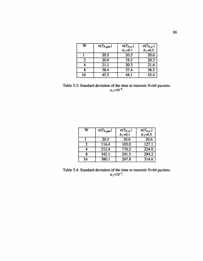
Table 5.3: Standard deviation of the time to transmit N=64 packets. a *=lo4.

Table 5.4: Standard deviation of the time to transmit N=64 packets. a ,=lo-'.

once an error has occurred, we are more likely to be in an acute shortage of

buffers, than otherwise.

Table 5.1 shows the expected time to transmit N=64 packets with go-

back-n and selective repeat when al = and bl takes values from 0 to

0.5. The effect of bl is seen to be negligible in this case, even for high values

of bl . This is because a1 is so low that it is unlikely that the j + k packets

will have much effect on p(j, k) when k = 0. Since p(j, 0) remains low (see

Equation 5.12), the likelihood of hitting a state with k > 0 is very low, and

so the effect of bl is negligible for this case.

Increasing a1 does inflate the expected time, as we can see from Table

5.2, where we have put a1 = 10-l. The effect is more pronounced for larger

window sizes as one would expect: the larger the window size, the larger the

potential for congestion, and larger the potential for error. What is interest-

ing, and not necessarily obvious, is the sharp degradation in performance as

seen in Table 5.2. This is the network equivalent of thrashing. From Table

5.1, we note that the expected time decreases at first with respect to win-

dow size but then starts increasing again, implying that there is an optimum

point for the window size. In Table 5.2, that optimum is for w = 1. Thus

the optimum point of operating the window will change for different values

of a l . We are far from being the first to discover the potential for congestion

as window size increases: Jacobson, Ramakrishnan and Jain, [Jac88, RJ881,

have proposed dynamic window algorithms for the same purpose. Our con-

tribution, however, is to quantify the effect of window size on the congestion

level, and to corroborate the fact that larger windows do have a detrimental

effect on performance when the network is congested (i.e., a1 is high).

In Table 5.3 and 5.4, we tabulate the standard deviation of the time to

transmit N = 64 packets for the same two values of a1 as before. Notice that

the standard deviation also gets worse with higher a1 , and this effect is again

more pronounced for larger windows. A comparison of go-back-n and selec-

tive repeat shows that go-back-n performs roughly equal to selective repeat

when bl = 0.5. One would normally expect selective repeat to perform better

if bl is low, because that implies that an error does not significantly affect

gbn 0.5 /

the 'state' of congestion. If, however, bl is high, transmitting more packets

when an error has occurred can only worsen the congestion in the network.

100 I I I I I I 1 I I 1 I I I I I 1

0 1 2 3 4 5 6 7 8 9 1 0 1 1 1 2 1 3 1 4 1 5 1 6 W

Figure 5.4: Expected time vs window size N = 64.

pb = 0.1 and 0.5, t l = 1.0.

Even selective repeat is seen to perform very poorly because associated with

an error is the cost of detecting it. Retransmissions are therefore expensive.

Let us next consider the more concrete error model that we had discussed

in Section 5.2. This was the single node model with finite buffers, carrying

some 'background' traffic when a multi-packet message arrives. The packets

in the message are assumed to arrive tl units of time apart. The parameters

of this model are pa, the background traffic intensity, tl , the spacing between

packets of the foreground message and K the number of buffers at this node.

We let K = 8 in our experiments and vary pa and t l . Figure 5.4 shows the

time to transmit N = 64 packets using go-back-n and selective repeat for

pb = 0.1 and 0.5 and tl = 1.0. Qualitatively, our conclusions are the same as

before: when the system is thrashing (and losing packets), the performance

is poor; while selective repeat may be slightly better, there is not much to

write home about. On the other hand, when the system loses relatively few

packets, go-back-n can match the performance of selective repeat.

5.6. Conclusions

In this chapter, we studied the go-back-n and the selective repeat proto-

cols when packet errors were due to congestion loss. Specifically, we studied

the effect of window size on performance.

We developed congestion models and protocol models to evaluate the

two retransmission strategies. The performance measures that we considered

were the expectation and the standard deviation of the time to completion

of an N-packet transfer.

We considered two separate congestion models, an abstract one and a

concrete one. In the abstract model, congestion dependent errors were a

function of the current congestion level in the system. We denoted this by

p(a) for a congestion state a . The choice of retransmission strategy may

depend on this function. We tried some alternative functions for p(cr) to

determine how the two protocols compared. First we tried a function which

represented a low congestion level and then one which represented a rela-

tively higher congestion level. We found that, irrespective of retransmission

strategy, the expected time as well as the standard deviation of the time to

transmit N packets increased sharply if the window size were large in the face

of heavy congestion. This was the network equivalent of thrashing. We also

saw the relative merits of the two retransmission strategies in these cases. If

the congestion level was low, (cf. a1 small in Section 5.5), the two retransmis-

sion strategies performed similarly. Under heavy congestion, it all depended

on the value of the probability of back-to-back errors. Even if selective re-

peat was better, the difference was in the region where the performance was

already substantially bad.

The concrete congestion model that we considered consisted of a finite

queue with some background traffic level. We derived the correlated error

patterns of a multi-packet message arrival when the packets of this mes-

sage were separated by some predetermined deterministic interval. These

probabilities were then used to drive the go-back-n and the selective repeat

protocol models. The conclusions of this study was no different. The degra-

dation due to large windows was much more pronounced, suggesting that

flow control, and not retransmission strategy, is really the important issue

under congest ion.

Determining the congestion function p ( a ) is at the moment an open

problem. It will depend on details of the system architecture like the number

of buffers at each point in transit, the timing characteristics of incoming and

outgoing links, the background traffic, etc. An experimental study using

statistical techniques seems like a viable approach to determine the function

p ( a ) . We are pursuing this avenue.

The performance of congestion control strategies also needs to be investi-

gated. In the next chapter, we present some of our results on the performance

of dynamic congestion control strategies that are based on explicit or implicit

feedback.

Chapter 6

Analysis of Dynamic Congestion Control Protocols - A Fokker-Planck Approximat ion

6.1. Introduction

In this chapter we investigate the performance of congestion control

protocols that dynamically change input rates based on feedback information

received from the network. This is motivated by recent proposals for adap-

tive congestion control algorithms [Jac 88, RaJa 88,901, where the sender's

window size at the transport layer is adjusted based on perceived congestion

level of a bottleneck node.

We develop, from first principles, a Fokker-Planck-like equation for the

evolution of the joint probability density function of queue length and ar-

rival rate at the bottleneck node. This approximates the transient behavior

of a queue subjected to adaptive rate-control. We then seek answers to ques-

tions regarding stability (or oscillations) and fairness of a particular adaptive

algorithm. We also investigate the effect of delayed feedback; on performaxlce.

We find that, in the absence of feedback delay, senders using the

Jacobson-Ramakrishnan- Jain (or JRJ) Algorithm [Jac 88, RaJa 88,901 (or

rather, an equivalent rate-based algorithm) converge to an equilibrium. Fur-

ther, this algorithm is fair in that all sources sharing a resource get an equal

share of the resource if they use the same parameters for adjusting their

rates. The exact share of the resource that different sources get when they

use different parameters is also determined.

A delay in the feedback information is shown to introduce cyclic behav-

ior. If different sources get the feedback information after dif irent amounts

of delay, then the algorithm may also be unfair, i.e., the sources may get

unequal throughput. In a simulation study of the JRJ-protocol, Zhang ob-

served oscillations in the queue length at intermediate nodes [Zha 891. She

also observed that connections with larger number of hops received a poorer

share of an intermediate resource than those with a smaller number of hops.

Jacobson also observed this independently in his measurements [Jac 881. Our

analysis not only concurs with these results, it also explains their reasons.

The oscillations are due to delayed feedback; the unfairness is partly due to

the larger (feedback) delay suffered by the longer connections as compared

to the shorter ones.

The rest of this chapter is organized as follows. Section 6.2 presents the

model. In Section 6.3, a Fokker-Planck approximation for the time dependent

queue behavior is derived. Section 6.4 discusses the properties of the JRJ-

algorithm when only one source is using the resource. Section 6.5 investigates

the properties of the system with multiple sources. Section 6.6 re-investigates

these properties in the presence of delayed feedback. Section 6.7 presents our

conclusions.

Model

The model we have chosen is motivated by the Jacobson-Ramakrishnan-

Jain Algorithm for window adjustment. In the JRJ algorithm, when conges-

tion is detected (by implicit or explicit feedback), the window size is decreased

multiplicatively. However, when there is no congestion, it is increased linearly

- to probe for more bandwidth, i.e.,

+ { I d ; if congested; w + a; if not congested.

While this makes good intuitive sense, it is far from clear as to what

values the parameters a and d should take. Further, it is not provably clear

if the algorithm is fair or stable1 and if so, under what circumstances.

To understand the behavior of dynamic congestion control algorithms,

we study a queueing system with a time varying input rate. The latter is

adjusted periodically based on some feedback that the end-point receives

about the state of the queue.

We are interested in the time evolution of the queue length density

function. Let us assume that we are changing the arrival rate, X(t), based

on the current queue length, Q(t), at some bottleneck node. An example

adaptive control algorithm could be

where ij is some target queue length. Co and C1 are positive constants.

Equation 6.2 models a linear increase in X for Q(t) 5 tj and an expo-

nential decrease in it for Q(t) > q. It is therefore the rate-analogue of the

dynamic window adjustment algorithm given by Equation 6.1. For purposes

of generality however, we shall denote

g ( . ) can be viewed as a generic rate-control algorithm.

To analyze the effect of Equation (6.2), Bolot and Shankar [Bosh 901

used two separate differential equations, one for the queue length, Q(t), and

another for the arrival rate X(t). They then coupled these two together by

letting X(t) drive the differential equation for Q(t) and vice-versa. This

works fine when Q(t) and X(t) are both determinist ic , as is the case in their

model. Suppose, however, that Q(t) were a random variable and say, we were

An algorithm is fair if everybody gets a 'fair' share of the resource (Fair share and equal share are synonymous if all the demands are equal). Stability, on the other hand, implies that the algorithm converges to a particular value.

observing the process {(Q(t), X(t))) as time progressed. Given some initial

values (Q(O), X(O)), let the queue length at time t be Q(t) = q, for some q.

At this point, the value of X(t) is dependent on not just the current value of

q, but also on the sample path of Q(s), 0 5 s 5 t. Intermediate values of the

queue length afFects X because of Equation 6.2 and since the sample path of

Q is random, X(t) itself is a random variable. Coupling the two equations

seems difficult now.

We therefore choose an alternate route. Let p be the average service rate

of the queue and let v(t) = (X(t) - p) be the instantaneous queue growth

rate (with the convention that v(t) = 0 if Q(t) = 0 and X(t) < p). We define

f (t, q, v) to be the joint probability density function of (Q(t), v(t)). Our goal

is to understand the time dependent behavior of f (.) based on g(.) and the

variabilities of Q(t) and v(t). We investigate this in the next section. The

result is a Fokker-Planck like equation for f (t, q, v).

6.3. Fokker-Planck approximat ion for queue with feedback control

Suppose that at time t, the queue length and queue growth rate are

given by Q(t) = i and v(t) = C. We want to express the density function

f (t + T, q, v) in terms of f (t, 6, i.). We assume that variability in v is caused

only by the random sample path of Q and there is no 'intrinsic' variability

in v. Then, given Q(t + T) = q, and some small T,

Let h(t + T, q, vlt, i , fi) be the conditional probability of the transition

between ( i , C) and (q, v) in time time (t , t + T). Then by the law of total

probability,

The integral over fi in Equation 6.5 is essentially a delta function which is

zero for all values of 6 except that satisfying Equation 6.4. We then have2

with the understanding that fi and v are related by Equation 6.4. The factor

1 + gy T in the denominator is the derivative of v(t + T) with respect to fi and

serves to preserves the conservation of probability.

Now, let us further assume that the central limit theorem holds approx-

imately for the conditional density function h(-), i.e.,

where a2 is the variance of Q. Validity of this assumption is key to the

Fokker-Planck approximation that follows.

Combining Equations 6.6 and 6.7 gives

To derive the differential equation of f (.) with respect to time, we subtract

f (t, q, v) from both sides, divide by T and let T + 0. We then get

Let

T--+0 T (6.10)

2 notation: gv = dgldv, fi = d f /at, fq = d f ldq, fpg = d2 f /dq2 etc.

higher order moments may be needed t o express more burstiness in h.

Adding (and subtracting) f (t, q, t ) to (and from) the right hand side of this

equation, we get

(6.11)

The first integral in Equation 6.11 is the same as in the typical Fokker-Planck

equation, see [New 68, New 71, Kle 761. As T tends to 0, then t must tend

to v, (see Equation 6.4)) and this integral becomes

The second integral is equal to

Combining Equations 6.9, 6.10, 6.11, 6.12 and 6.13, and noting that g, f + gfv = (gf )U? we have

Equation 6.14 describes the basic equation of motion for the density function

f (9.

6.4. Properties of Algorithm 6.2

We now investigate the properties of Algorithm 6.2 in conjunction with

Equation 6.14. For the purposes of an intuitive discussion, we suppress the

o2 term in Equation 6.14 and study a reduced system. We therefore have

a hyperpolic partial differential equation whose properties can be explored

by studying its characteristics. Consider the q - v diagram of Figure 6.1.

The x-axis represents the queue length, Q, and the y-axis represents the

instantaneous queue growth rate, v. Two lines corresponding to Q = ij and

v = 0, shown by dotted lines, divide the q - v plane into four quadrants.

The behavior of Equation 6.14 is best described by considering each quadrant

separately.

First consider Quadrant I in Figure 6.1. This corresponds to v > 0 (i.e.,

X > p ) and Q < q. Since X > p, the instantaneous queue length at any

point in this quadrant is increasing. The instantaneous v is also increasing

because dX/dt = Co > 0. The resultant direction of instantaneous motion

(i.e., the characteristic) is increasing in both Q and v as shown in the figure.

Notice that Equation 6.14 confirms this intuition: the coefficient of f, which

represents the Q-drift is v and this is positive in Quadrant I; the coefficient

of f, which represents the v-drift is g ( . ) = +Co which is positive as well.

The characteristic is the resultant of these two drifts.

Next, consider Quadrant 11. Here Q > q and Y > 0 (i.e., X > p). From

Equation 6.14, the Q-drift is again positive since v > 0. However, the v-drift

is now negative because dX/dt is -CIA for Q > ij. The characteristic, which

is the resultant of these two drifts, is increasing in Q but decreasing in v as

shown in Figure 6.1.

We can similarly check that in Quadrant 111, both the Q-drift and the

v-drift are negative while in Quadrant IV, the Q-drift is negative but the

v-drift is positive. The directions of individual drifts and the characteristics

are shown in the figure.

Now, suppose we were to trace the path of a 'particle' that obeys both

Equation 6.14 and Equation 6.2. This path will follow the characteristic.

Therefore, from the above argument, it is clear that the trajectory would

either be a cycle or a spiral; the latter could be one that converges inwards

or diverges outward. Further, a convergent spiral could home in to either a

limit point or a limit cycle. Theorem 6.1 below says that the path of any

particle obeying Equations 6.2 and 6.14 (ignoring the a2 term) is a convergent

Figure 6.1: Characteristics and their directions.

Figure 6.2: Converging spiral.

cycle with the limit point Q = q and v = 0. Notice that this is exactly the

desired point of operation of the adaptive algorithm.

Theorem 6.1: If a2 = 0 in Equation 6.14, then Algorithm 6.2 converges in the limit.

The limit point is q = t j , X = p. This result is due to Prof. John Strikwerda.

We have

and

Since p, the average service rate, is not changing with time,

Now, suppose that at time t = 0, X is some value Xo which is less than

p and q is q (see Figure 6.2). From Equation 6.17, we have

Its solution is

After a certain time, say tl , the characteristic hits q = ij line again. Let X be

X1 now. For the moment, let us assume that the characteristic did not hit

the q = 0 boundary, so that Equation 6.18 is valid all the way upto t = tl . The two roots of Equation 6.18 with q = q are t = 0 and t = 2(p -

Xo)/Co. The first one corresponds to the initial point. Therefore,

Also, since X = p + dqldt, we have, from Equation 6.18 and 6.19,

A1 = p + Cot1 + (Xo - p)

= 2p - Xo (6.20)

Notice that X I - p is equal to p - Xo which says that the overshoot above p

is exactly equal to p - Xo, irrespective of the value of Co. This is therefore an

inherent property of the linear increase component of Algorithm 6.2.

Let us next evaluate the characteristic when q is greater than q. We have

and

Since at t = t l , q = q and dqldt = X1 - p, its solution is

Let the characteristic again hit the q = q line at some later time t2 and

let X now be X2. Then from Equation 6.23, we have at time t2 ,

Putting a = Cl(t2 - t l ) , we get

Since dqldt is equal to X - p, X2 can be obtained by differentiating Equation

6.23. We get

Substituting the value of X1 from Equation 6.20, we have

Therefore

The question then is whether X2/Xo is greater than 1, less than 1 or equal to

1. From Figure 6.2, we see that if A2/X0 were greater than 1, we would have

a converging spiral. We verify next that this is indeed the case.

Let y = p / X I in Equation 6.24. Then, using Equation 6.20, we have

Substituting into Equation 6.27, we get

From Equation 6.24, y is given by

Therefore,

and from 6.29 and 6.30,

Let us next define a function, h(a), such that

If h(a) is less than 0, then from Equation 6.31, X2/Xo is greater than 1.

Notice that h(0) is 0 and

Differentiating once again,

h1I(a) = -ae-" < 0 for a > 0

Therefore,

Similarly,

From Equations 6.31, 6.32 and 6.33, we have

which implies that the spiral is convergent.

So far, we have assumed that the characteristic starting at ( q , Xo) never

hits the q = 0 boundary. In this case, we have established that we have a

convergent spiral. To complete the proof, let us next consider the case when

a characteristic hits the left boundary, q = 0.

Notice that this characteristic cannot hit the boundary for X > p, be-

cause the q-drift which is positive for X > p, will pull it to the right. There-

fore, if it hits the q = 0 boundary then X < p. Suppose that for some

initial (q , io), the characteristic barely touches the boundary. This point is

(q = 0, X = p), as shown by arc 'a' in Figure 6.3. Since Equations 6.18,

6.19 and 6.20 hold for this characteristic, it will converge by the earlier argu-

ment. Any point corresponding to Xo < &, first hits the q = 0 boundary (as

shown by arc e), then goes vertically up until X = p, (arc f ) , and then fol-

lows the characteristic corresponding to i o , (arcs b, e, d). This too, therefore,

converges. The ~ d e 6.14 is however, not quite valid in this range.

This completes the proof of Theorem 6.1. 1

Corollary 1: If both the increase and the decrease components are linear,

then the system will never converge.

Pro0 f :

We saw from Equation 6.20 that the amount of overshoot exactly equals

the amount of undershoot during the linear increase phase irrespective of the

value of Co. The same is true in the reverse direction for a linear decrease

algorithm. Hence, the system moves in a non-convergent cycle. 1

Equation 14 can be used to simulate the behavior of systems by us-

ing a finite difference approximation. Thus given an initial density function

f (0, q, v), one can determine the density function at some later time t . The

finite difference schemes required for this need to be considerably sophes-

ticated so as to ensure stable and accurate solutions. We are working on

this currently and would report the results at a later time. Preliminary re-

sults show that while convergence is guaranteed by Theorem 6.1, the time

to convergence can be quite large unless Co and Cl are large.

6.5. Multiple Sources

We have assumed so far that there is only a single source transmitting

through a particular node. We next investigate the properties of the system

with multiple sources. Specifically, we are interested in the convergence and

fairness properties when multiple sources compete for a resource. There are

Figure 6.3: Converging spiral when characteristics touch the q=O boundary.

Figure 6.4: Meaning of Atl,At2 and At3.

two 'feedback schemes' that we consider; one where all the sources receive

the (same) cumulative queue length information [RaJa 88, Jac 881 and an-

other, where each source receives its own queue length information only.4 In

the latter case, fairness is guaranteed by the scheduler; the analysis of the

previous sections then apply directly to each source; if there are n sources,

we change p to ,u/n and apply Equations 6.2 and 6.12. The conclusion is

that the system is both convergent and fair.

Next, let us consider the case when all sources receive the common queue

length information. All of them adjust their rates according to Algorithm 2.

If there are n sources, let (Al (t), AS (t), , A n (t)) denote their transmission

rates at time t. Let X(t) = EL1 X,(t) be the cumulative transmission rate

and let Q(t) be the cumulative queue length at time t . Then

This is the equivalent version of Equation 6.2 for multiple sources. Equations

6.12 and 6.35 completely specify the behavior of the system. From Theorem

6.1, this system of multiple sources converges. Notice that the increase rate is

proportional to n, but the decrease rate is unchanged. Therefore, the length

of the spiral trajectory (the path to convergence) is the same, but the time

to traverse it is shortened (see Equations 18 and 19).

We next investigate if Algorithm 6.35 is fair. If it is, then the Xis must

be equal to each other in the limit.

Theorem 6.2:

Algorithm 6.35 is fair.

Pro0 f :

The proof is due to Prof. John Strikwerda.

For the purposes of this proof, let us assume that the different sources use

different increase and decrease parameters. Suppose there are n sources

possible with a Fair-Queue-like scheduling algorithm a t the resource.

this is therefore, a more general proof.

and let source i use an increase parameter Co,i and a decrease parameter

C1,;. Let X1, X2, . , An denote their respective transmission rates in the limit

(notice that convergence is guaranteed by Theorem 6.1). Then

Suppose A!, A:, . - . , X: are the transmission rates at some time such that

but let q be greater than q (see Figure 6.4). Let Atl, At2 and At3 be as

shown in the figure. These are three disjoint segments of the time to complete

one complete cycle.6 Let X i , X i , - - - , A: be the new values of the Xis at the

end of the cycle. Then, the equation for X i is given by

Other Xi's are similar. We then get,

Let y = (Atl+At3)/At2. Then passing Equation 6.37 to the limit as At2 -+ 0

which will occur as the processes tend to equilibrium, we get

Similarly,

In the limit, when convergence occurs,

i.e., when the process hits X = p and q > q again.

Figure 6.5: Delayed feedback.

Figure 6.6: Consequence of delayed feedback.

Since, xi X i = p, we have

Therefore

Thus, if the Co,;'s and the Cl,i's are equal, then X i = p/n, which implies

complete fairness. I

In real systems, this may be violated because the sources get the feed-

back information after different amounts of delay and due to finite queue

capacity.

6.6. Effect of feedback delay

We next investigate the effect of feedback delay on the control algorithm.

Figure 6.5 shows the mechanics of the system; r is the delay in obtaining the

feedback information from the queue to the control point; d is the inertia in

the forward direction in that it takes the control algorithm this much time

to take effect after X is changed. Let us, for the moment, assume that d is 0.

The control algorithm can now be precisely stated as:

It turns out that this algorithm does not converge. To see this, suppose

that at time to, the process is at the target equilibrium point Q(to) = Q

and X ( t o ) = p. We shall show that it cannot remain here for any significant

amount of time.

We need to consider two cases. First, let us say that the process arrived

at this point from the left, i.e., Q(to - r ) < ij. Then

dX(t)/dt = Co, t E (to, to + T) (6.43)

Therefore

X(to + r ) = q to ) + rCo = p + r Co > p (6.44)

and

Figure 6.6 shows this pictorially (see Quadrant 11). The process overshoots

the equilibrium point because r > 0.

Next, let us consider the case when the process arrives at (ij, p) from

the right, i.e., Q(to - r) > ij. Then

dA(t)/dt = -CJ ( t ) , t E (to, to + T) (6.46)

Therefore

X(to + T) A(to)e-cl' = pe-C1' < p (6.47)

and P ~ ( t ~ + r ) = q - - ( r c l -l+edC1') < q (6.48) c1

Figure 6.6 shows this case too (Quadrant IV). The process, here, undershoots

the equilibrium.

Notice that the overshoot and the undershoot are going to be larger

than what is shown above because when Q(to) = ij, the value of X will either

be greater than p or less than p (depending on whether the process came

from left or right respectively). Clearly the system cannot stabilize at (ij, p).

Further, at any other point in the q - X space, the process is forced to be in

mot ion. Therefore the system oscillates.

These oscillations cannot however, become unbounded. To see this,

suppose the process is currently at (Ao, tj) and Xo is large. The function g()

is Co. At r time units later the control algorithm switches to the exponential

decay phase. After some time, say Atl, the process hits the q = ij line again.

Another r time units later it switches to the linear increase phase. Let this

point be ( A l , ql). Then

During the linear increase phase, the process once again hits q = ij line (say,

after time Atz). Let the value of X now be X2. Then

Notice that At2 is bounded because X1 > 0 and q l > 0. Hence, X2 is bounded

from above. This means that if Xo is large, the diameter of the oscillation

has to shrink in the next cycle. This, together with the fact that there can

be no stable point, proves the existence of a limit cycle.

The diameter of the oscillatory cycle increases with the delay, r. If differ-

ent sources experience different delays, they have different oscillatory cycles.

This could lead to unfairness in resource usage.

Equations 6.44, 6.45, 6.47 and 6.48 point to an important difficulty

with choosing parameters Co and C1. The oscillations are larger with higher

values of of these parameters. Thus, while larger values of Co and Cl help

to converge faster in the absence of delay (see Equation 6.18 for example),

they cause larger oscillations in the presence of delay.

Next, let us consider the effect of the inertia d. We still have

However, d2Q/dt2 is now given by

i.e., the queue length now lags r + d time units while X still lags r time units.

The oscillatory effect is now more severe, but qualitatively similar to the

previous case, i.e., larger values of Co and C1 cause larger oscillations.

6.7. Summary and conclusions

We presented an approximate analysis of a queue with dynamically

changing input rates based on implicit or explicit feedback. This was moti-

vat ed by recent proposals for adaptive congestion control algorithms [RaJa

88, 90, Jac 881, where the sender's window size at the transport level was

adjusted based on perceived congestion level of a bottleneck node. We de-

veloped an analysis methodology for a simplified system; yet it was powerful

enough to answer the important questions regarding st ability, convergence

(or oscillations), fairness and the significant effect that delayed feedback plays

on performance. Specifically, we found that, in the absence of feedback

delay, the linear increase/exponential decrease algorithm of Jacobson and

Ramakrishnan-Jain [Jac 88, RaJa 881 was provably stable and fair. Delayed

feedback, on the other hand, introduced oscillations for every individual user

as well as unfairness across those competing for the same resource. While

simulation studies of Zhang [Zha 891 had observed the oscillations in the cu-

mulative queue length at the bottleneck and measurements by Jacobson [Jac

881 had revealed some of the unfairness properties, the reasons for these had

not been properly understood. We identified quantitatively the real cause for

the these effects.

We found that introduction of feedback delay however added oscillations

which settle down to a l imi t cycle, i.e., a cyclic pattern that was constant

in the limit. This cyclic pattern agreed with simulation results by Zhang

[Zha 891. The proof of the existence of a limit cycle, we believe, is a new

result. The diameter of the limit cycle (or equivalently the magnitude of

the oscillations) was seen to be sensitive to the parameters Co, Cl and the

feedback delay. For instance, for a fixed Co and feedback delay, a larger C1

increased this diameter. So, while in the absence of feedback delay, a larger

C1 boosted the speed of convergence, in the presence of delay, it caused

wilder oscillations. The size of the oscillations also increased with Co and

feedback delay.

Our model is fairly general and is applicable to evaluate the performance

of a wide range of feedback control schemes. It is an extension of the classical

Fokker-Planck equation. Therefore, it addresses traffic variability (to some

extent) that fluid approximation techniques do not.

Chapter 7

Future Work

Introduction

In this chapter, we outline our plans for future research. We wish to

explore two major avenues in the near future.

One avenue is congestion control in high speed wide area networks. The

other is extending the Fokker-Planck analysis of feedback control algorithms

with delay in the feedback path.

7.2. Congestion control in high speed, wide area networks

Introduction of optical fibers is pushing transmission speeds to the gi-

gabit range. While this offers new dimensions to networking, the challenge

we face is to pass these hardware speeds to the applications that will use

it. A stiff performance hurdle is the high bandwidth-delay product of these

networks when propagation delay is large. The round trip propagation delay

across continental USA in fiber is approximately 46 msec. At gigabit speeds,

one could dump 10' * 46 * lov3 bits (= 5.75 MBytes) of data into the net-

work before hearing from the receiver. Consider now, a reactive congestion

control scheme that uses (implicit or explicit) feedback information from the

network to adjust the input transmission rate. The feedback information is

potentially old in this environment, relative to the duration of short-term

fluctuations in queue length caused by bursty traffic. (Feedback may still

be used to track long term fluctuations in traffic). To deal with short term

bursts, numerous 'open-loop' strategies have recently been proposed [Zha

89, SLCG 89, Tur 86, BCS 90, Go1 901. We propose a new strategy which

we believe will perform better. A careful comparative study needs to be

performed however, to get concrete performance answers.

Before we delve into the details of open-loop control, we take a closer

look at the problem of packet loss once more. We shall then address possible

solution methods including those that have been proposed recently by others.

The Problem

Suppose that a message of size N packets is being transmitted over a

network. Let pj be the probability of packet loss for packet j with a particular

flow control protocol and a particular retransmission strategy. Let T be the

average cost of an error. If the pj were statistically independent and identical,

we know from Chapter 3 that the expected time to transmit the N-packet

message will be P j E[TN] = E[Th',NoErrs] + N -

1 - ~ j

If errors were correlated however, we get a weaker relation. Let p = supj pj.

Then P

E[TN] 5 E[TN,NoErrs] + N-7 1 - P

E[TN,NoErrs] + NPT

because p < < 1 . Let us define loss of efficiency, q, as

Then, using the relation EITN,NoErrs] = Ntl + tend, (C f . Chapter 3), we

have

rl I NP7 I

Ntl + t e n d

This relation shows quantitatively, how efficiency scales (or decays) with

transmission speed. For the go-back-n protocol, T is at least equal to the

roundtrip propagation delay. Increase in transmission speeds to the gigabit

range would decrease tl 10 to 100 fold, so p would have to decrease by the

same amount to keep efficiency comparable.' Equation 7.1 is therefore a

'rule-of-thumb' design equation.

For selective repeat, the value of T depends on N and flow control. If

the pipe were kept full for significant amounts of time, the cost due to the

loss of a packet would be low. However, this would be difficult in high speed

environments on two counts. First, most message bursts would not be large

enough to keep the pipe full. Second, high bandwidth-delay product would

require large receive buffers for caching out of order data.

The solution that we seek is to reduce packet loss without introducing

negative side effects like increased queueing delays or slowing down transmis-

sions unnecessarily. To this end, let us first consider some of the proposals

that have been made recently.

Related Work The Leaky Bucke t Protocol [Tur 86, SLCG 891 provides a bucket of finite

size at the input. The bucket is supplied with tokens which arrive at some

specified rate y. Tokens which arrive when the bucket is full are discarded.

When packets from a user arrive, they each grab a token (if available) and

The 5 sign in Equation 7.1 does not make this argument any weaker. It can easily be checked that 77 R .p jr / t l . Consider next a loss-curve for p j vs j . A higher value of p = supj p:s liiely to increase all the pj's because they are

congestion-related.

get in the network. If the bucket is empty, the packet waits for a new token

to arrive and only then does it have permission to go in.

The Generalized Leaky B u c k e t Protocol [BCS 901 provides two buckets

at the input instead of one. These are called the Green Bucket and the Red

Bucket and are fed at rates yg and y, respectively. An incoming packet

grabs a token from the green bucket if the latter is non-empty and enters the

network. Otherwise, it tries the red bucket, failing which it waits. Packets

with green tokens are given a higher priority at intermediate queues. The

idea of Generalized Leaky Bucket is to allow users to exceed the one-level

burst size, but at their own risk. The important problem is to determine what

yg and y, should be, to ensure low loss rates and yet higher throughput. No

such study has yet been reported.

The Vir tua l Clock Protocol [Zha 891 takes the approach of allocating part

of intermediate resources to individual users based on their average demands.

It is a reservation based scheme. Let us suppose that a user (or a 'flow' as

Zhang calls it) i is allocated a rate Xi. Each node associated with this user

maintains a virtual clock vi which determines user i's priority with respect

to other competing users. Initially, vi is set to the real clock. When a packet

belonging to user i arrives, vi is incremented to v; + l/Xi. The packet that is

scheduled next for dispatching belongs to the user with the minimum virtual

clock.

The Leaky Bucket Protocol allows bursts of up to size K at the en-

trance to the network. Intermediate nodes could however see larger burst

sizes due to cumulative effect of multiple bursts from different users. Thus

this protocol offers only limited protection from buffer overruns and large

queueing delays. The Virtual Clock Protocol on the other hand maintains

traffic smoothness across tandem links if the traffic is smooth at the entry

point. However, in so doing, it forces bursty sources to transmit at their

average rates or face the penalty of large delays and/or packet loss.

S top -and-Go Queueing [Gol 901 ensures that the smoothness of traffic

at the input is maintained across multiple hops. While Golestani proposed

it for real-time traffic, it is relevant to data traffic as well. The basic idea of

Stop-and-Go Queueing is to slow down traffic on a per user basis at every

intermediate node so that packets which were separated out at the input

do not arrive in close succession at some node in the network. This latter

phenomenon could occur if successive packets of a user get queued at some

intermediate node. Golestani shows that Stop-and-Go Queueing can ensure

lossless transmission with a bounded number of buffers. Unfortunately this

is at the expense of throttling traffic, possibly unnecessarily.

Notice that, unlike Virtual Clock, Stop-and-Go Queueing is not a pri-

ority scheduling algorithm. In Virtual Clock, the average specified rates of

individual users are used to determine who goes next. If a user transmits

faster than its specified average rate, it still gets scheduled if the resource

is free. This is not possible with Stop-and-Go Queueing. On the other

hand, Stop-and-Go Queueing does allow users more flexibility with respect

to defining their smoothness (the average rate over a time period T).

New Proposal

We propose the Gate Protocol which combines the ideas of Leaky Bucket

and Virtual Clock to provide good service to packet trains [RoJa 86, SoLa

881 across tandem links. In the packet train model for data traffic, a user is

assumed to be in one of two states. In one state it transmits data with some

rate A. In the other, it remains idle. Let us suppose that a user i specifies

its transmission rate Xi, and its burst characteristics tl l i and t2,, as shown in

Figure 7.1. Xi corresponds to the speed that user i wishes to transmit at. It

may be the maximum speed at which it can transmit or the speed decreed by

flow control. We believe that users would be able to specify their packet-train

characteristics with the help of statistics collectors. Further investigation is

required to determine the accuracy of these predictions.

The Gate Protocol will work as follows. Let Ni = Xitlti/packet size. Ni

is the number of packets that user i would transmit in time tlli. Associate a

virtual clock v, and a bucket B; at every node in the path of user i. Initialize

t1.i t2.i

Figure 7.1. User specifications for Gate.

B; to Ni and vi to real clock.

When a packet from user i arrives at the node, execute the following

algorithm.

priority [packet] := vi

If ( Bi > 0) then

vj := v; + l / X i

Bi := B i - 1

end

else

v; := V, + t2,;

B; := Ni

end

{ schedule packet with the minimum priority )

If a user behaves according to its own specifications, this scheduling al-

gorithm can guarantee it good service in that its packets will get dispatched

without excessive delay. Also, packet loss can be avoided altogether. How-

ever, if a user exceeds its specified burst size or transmits faster than agreed

upon, then as in Virtual Clock, its priority is reduced and its own perfor-

mance is affected.

Notice that Gate is identical to Virtual Clock if t2,i = 0 (In this case,

N; could be any positive integer). Thus Gate allows users to specify only

their average rates of transmission if they choose to. However, if a user

provides more information to the network, it could get better service than

either Virtual Clock or Leaky Bucket. Also, unlike Stop-and-Go, it does

not throttle packets when a resource is idle. Therefore, it will deliver higher

throughput and lower packet delays than Stop-and-Go. Gate and Virtual

Clock also provide protection from misbehaving users. Stop-and-Go does

not.

Outline of Performance Study

We plan to compare the performance of these protocols using detailed

simulation. The workload will be the number of users and their burst char-

acteristics. The output of interest would be effective throughput, loss and

delay as a function of offered load.

A subsequent study would be to determine analytically the tradeoffs

involved in exceeding the specified rates as a function of congestion level.

Design of optimistic versions of the protocols at the input would benefit

from this information. One advantage in this reservation-based environment

is that the nodes are aware of rough user demands. If they could compute

levels of loss probabilities as a function of user demand, they could pass the

information to the users. Since users are likely to persist longer than just

a round-trip delay, the feedback information may be exploited to get better

performance. Users could decide if they want to exceed their rates because

they are aware of the costs associated with it.

Once the loss probabilities are determined, we would compare 'Opti-

mistic' Gate with Generalized Leaky Bucket and 'Optimistic' Virtual Clock

using simulation.

7.3. Fokker-Planck analysis of feedback control with delay

We would also explore ways to extend the Fokker-Planck analysis of

Chapter 6 with a delayed feedback. At this point, the problem looks quite

formidable and we do not know how we would go about solving it.

Bibliography

[AnPr 861 : Anagnostou, M.E. and E. N. Protonotarios, "Performance

analysis of the selective repeat ARQ protocol," IEEE Trans.

Commun., vol. COM-34, pp. 127-135, Feb. 1986.

[BCS 901: Bala, K., I. Cidon and K. Sohraby, "Congestion Control in

High Speed Packet Switched Networks,'' Proc. of the IEEE

Infocom, pp 520-526, June 1990.

[Bir 811: Birrel, N.D., "Pre-emptive retransmission for communication

over noisy channels," IEE Proc., Part F, vol. 128, pp 393-400,

Nov 1981.

[BPS 881: Bolot, J.C., B.D. Plateau and A. U. Shankar, "Performance

analysis of transport protocols over congestive channels," Tech

Report UMIACS-TR-88-22.1 CS-TR-2004.1, Department of

Computer Science, University of Maryland, Revised August

1988.

[BrMo 863: Bruneel, H. and M. Moeneclaey, "On the throughput analysis

of some continuous ARQ strategies with repeated transmis-

sions," IEEE Trans. Commun., vol. COM-34, pp. 244-249,

March 1986.

[BRT 881: Blake, J.T., A.L. Reibman and K.S. Trivedi, LLSensitivity Ana-

lysis of Reliability and Performability Measures for Multipro-

cessor Systems," Proc. of the ACM Sigmetrics, pp 177-186,

May 1988.

[FKYN 781:

[Gol 901:

[Gus 871:

[Jac 881:

[Jaf 81a]:

[Jaf 81bl:

Fujiwara, C., M. Kasahara, K. Yamashita and T. Namekawa,

"Evaluations of Error Control Techniques in Both Indepen-

dent Error and Dependent-Error Channels," IEEE Trans.

Commun., vol. COM-26, pp 785-794, June 1978.

Gaver, D.P., Jr., "Diffusion Approximations and Models for

Certain Congestion Problems," Journal of Applied Probabil-

ity, pp 607-623, 1968.

Gerla, M. and L. Kleinrock, "Flow Control: A Comparative

Survey," IEEE Trans. Commun., vol. COM-28, pp 553-574,

April 1980.

Golestani, S. J . , "Congestion-Free Transmission of Real-Time

Traffic in Packet Networks," Proc. of the IEEE Infocom, pp

527-536, June 1990.

Gusella, R. , "The Analysis of Diskless Workstation Traffic

on an Ethernet," Tech. Rep. UCB/CSD 87/379, University of

California, Berkeley, November 1987.

Jacobson, V., "Congestion Avoidance and Control," Proc. of

the ACM Sigcomm, pp 314-329, Aug. 1988.

JafTe, J.M., "Bottleneck Flow Control," IEEE Trans. Corn-

mun., vol. COM-29, pp 954-962, July 1981.

Jaffe, J.M., "Flow Control Power is Nondecentralizable,"

IEEE Trans. Commun., vol. COM-29, pp 1301-1306,

September 1981.

[Jai 861: Jain, R., "A Timeout-Based Congestion Control Scheme for

[Jai 901:

[JaRo 851:

[JCH 841:

[KaCh 881:

[Kin 701:

[Kon 801:

[Kle 751:

[Kle 761:

Window Flow-Controlled Networks," IEEE Journal on Se-

lected Areas in Communications, pp 1162-1 167, 1986.

Jain, R,, "Congestion Control in Computer Networks: Issues

and Trends," IEEE Network Magazine, pp 24-30, May 1990.

Jain, R., and S. Routhier, "Packet Trains: Measurements and

a New Model for Computer Network Traffic," Tech Report

MIT/LCSTM 292, Department of Electrical Engg, MIT, Nov

1985.

Jain, R., D.M. Chiu and W.R. Hawe, L'A Quantitative Mea-

sure of Fairness and Discrimination for Resource Allocation

in Shared Systems," DEC Tech Rep TR-301, 1984.

Kanakia, H. and D.R. Cheriton, "The VMTP Adapter Board

(NAB): High-Performance Network Communication for Mul-

tiprocessors ," Proc. of the ACM Sigcomm, pp 175-187, Aug.

1988.

Kingman, J.F.C., "Inequalities in the Theory of Queues,"

Journal of the Royal Statistical Society, Series B, vol. 32, pp

102-110, 1970.

Konheim, A.G., "A Queueing Analysis of Two ARQ Proto-

cols," IEEE Trans. Commun., vol. COM-28, pp 1004-1014,

July 1980.

Kleinrock, L., Queueing Systems Vol I: Theory, John-Wiley

and Sons, New York, 1975.

Kleinrock, L., Queueing Systems Vol 11: Computer Applica-

tions, John-Wiley and Sons, New York, 1976.

[LaRe 791: Lam, S.S. and M. Reiser, "Congestion Control of Store-and-

Forward Networks by Input Buffer Limits - An Analysis,"

IEEE Trans. Commun., vol. COM-27, pp 127-133, Jan. 1979.

[LiYu 801: Lin, S., and P.S. Yu, "An Effective Control Scheme for Satel-

lite Communications," IEEE Trans. Commun., vol. COM-28,

pp 395-401, March 1980.

[MBC 841: Marsan, A., M.G. Balbo, and G. Conte, "A Class of General-

ized Stochastic Petri Nets," ACM Trans. Computer Systems,

vol2, pp 93-122, May 1984.

[MeSw 801: Merlin, P.M. , and P.J. Schweitzer, "Deadlock Avoidance in

Store-and-Forward Networks - I: Store-and-Forward Dead-

lock," IEEE Trans. Commun., vol. COM-28, pp 345-354,

March 1980.

[MiMi 901: Mitra, D. and I. Mitrani, "A Go-Back-N Protocol Which is

Efficient in High Speed Data Networks with Small Buffers,"

Proc. 4th Int'l Conference on Data Commun. Systems and

Their Performance, Barcelona, June 1990.

[MLS 901: Mukherjee, A., L.H. Landweber and J.C. Strikwerda, "Simul-

taneous Analysis of Flow and Error Control Strategies with

Congestion-Dependent Errors," Proc. of the A CM Sigmetrics,

May 1990.

[MLS 891: Mukherjee, A., L.H. Landweber and J.C. Strikwerda, "Eval-

uation of Retransmission Strategies in a Local Area Network

Environment," Proc. of the ACM Sigmetrics/Performance, pp

98-107, May 1989.

[Moe 861:

[Mor 781:

[Mor 881:

[MQR 871:

[New 681:

[New 711:

[Oht 891:

Moeneclaey, M., "Throughput optimization for a generalized

stop-and-wait ARQ scheme," IEEE Trans. Commun., vol.

COM-34, pp. 205-207, Feb. 1986.

Morris, J.M., "On Another go-back-n ARQ Technique for

High Error Rate Conditions," IEEE Trans. Commun., vol.

COM-26, pp 187-189, Jan. 1978.

Morgan, S., "Window Flow Control on a Trunked Byte-

Stream Virtual Circuit," IEEE Trans. Commun., vol. 36, pp

816-825, July 1988.

Mohan, S. , J. Qian and N.L. Rao, L'Efficient Point-To-Point

and Point-To-Multipoint Selective-Repeat ARQ Schemes with

Multiple Retransmissions : A Throughput Analysis," Proc. of

the ACM Sigcomm Workshop, pp 49-57, Aug. 1987.

Newell, G.F., "Queues with Time-Dependent Arrival Rates

1-111," Journal of Applied Probability, pp 436-451, 1968.

Newell, G.F., Applications of Queueing Theory, Chapman and

Hall Ltd., London, 1971.

Ohta, M., "Engineering of Congestion Control in a Large

Scale Network," Proc. 4th Int '1 Network Plannzng Symposium,

Palma de Mallorca, Spain, pp 301-305, Sept. 1989.

Ramakrishnan, K.K., and R. Jain, "A Binary Feedback

Scheme for Congestion Avoidance in Computer Networks with

a Connectionless Network Layer," Proc. of the ACM Sigcomm,

pp 303-313, Aug. 1988. Also, ACM Trans. Computer Systems,

vol. 8, pp 158-181, May 1990.

[Rei 791: Reiser, M., "A Queueing Network Analysis of Computer Com-

munication Networks with Window Flow Control," IEEE

Trans. Commun., pp 1199-1209, 1979.

[SaSc 801: Saad, S. and M. Schwartz, "Input Buffer Limiting Mechanisms

for Congestion Control," ICC, June 1980.

[Sas 751: Sastry, A.R.K., "Performance of Hybrid Error Control

Schemes on Satellite Channels," IEEE Trans. Commun., vol.

COM-23, pp 689-694, July 1975.

[SLCG 891: Sidi, M., W. Liu, I. Cidon and I. Gopal, "Congestion Con-

trol Through Input Rate Regulation," Proc. IEEE Globecom,

1989.

[SoLa 881: Song, C. and L.H. Landweber, "Optimizing Bulk Data Trans-

fer: A Packet Train Approach," Proc. of the ACM Sigcomm,

pp 134-145, Aug. 1988.

[SSSGJ 881: Sanghi, D., M.C.V. Subramaniam, A. U. Shankar, 0. Gud-

mundsson and P. Jalote, "Instrumenting a TCP Implementa-

tion," Tech. Report CS-TR-2061, Dept. of Computer Science,

University of Maryland, July 1988.

[Tan 8 11 : Tanenbaum, A.S., Computer Networks, Prentice-Hall Inc.,

Englewood Cliffs, NJ 07632, 1981.

[Tow 791: Towsley, D., "The Stutter Go-Back-N ARQ Protocol," IEEE

Trans. Commun., vol. COM-27, pp 869-875, June 1979.

[ToWo 791: Towsley, D. and J.K. Wolf, "On the Statistical Analysis of

Queue Lengths and Waiting Times for Statistical Multiplexors

with ARQ Retransmission Schemes," IEEE Trans. Commun. ,

vol COM-27, pp 693-702, April 1979.

[Tri 821: Trivedi, K.S., Probability and Statistics with Reliability, Queu-

ing, and Computer Science Applications, Prentice-Hall Inc.,

Englewood Cliffs, NJ 07632, 1982.

[Tur 861 : Turner, J ., "New directions in Communications (or Which

way to the Information Age?)," IEEE C o m m . Magazine, vol.

24, Oct 1986.

[Zha 891: Zhang, L., "A New Architecture for Packet Switching Network

Protocols," Ph.D. thesis, MIT, Dept. of Electrical Engg. and

Computer Science, Aug. 1989.

[Zwa 851: Zwaenepoel, W., "Protocols for Large Data Transfers on Local

Networks, Proc. of the A C M Sigcomm, pp 22-32, 1985.

Appendix 3.A

This section presents the analysis of the time to detect an error, as

discussed in Section 3.3.1. Given M+1 packets, of which the first packet has

failed, we are interested in the time the sender takes to detect the error. We

are assuming that errors due to electrical noise are much lower than errors

due to packet losses at the interface. In a single hop LAN, all packets are

received in the order sent. Therefore the receiver can detect a dropped packet

with sequence number s if it receives any packet with sequence number of

s + 1 or greater. It then NACKs sequence number s. If the NACK gets

through successfully, the error is detected at the sender; otherwise, a NACK

from a future packet is needed for error detection. Ultimately, if there are no

packets left (i.e., all M packets or their NACKs failed), the sender times out

after Ttimeout time units. So error detection at the sender is upper bounded

by Ttimeout .

Now let

qo = (1 - po), the probability that a packet does not fail.

~ = 1 - ~ ~ ~ , the probability that a packet exchange fails

Then,

Pr [i failures to detect] = (1 -u)ui, if 0 5 i 5 M - 1,

i f i = M . (3.A.1)

Distribution of time to detect

In the following discussion, C and T are defined as in Section 3.3.1. T, is the time to transmit a NACK packet, and Cn is the time to copy it from (to)

the interface memory to (from) the host memory. We assume that Cn 5 T . Let

Tatart = C + T

Tend'') = (C f T) f (C f Cn)

= (C + T) + (Cn + Tn) = (C + Cn) + (Cn + Tn)

Then the time to detect the error after exactly i failures, Ti is

Tstart + Tend "I + (i + I)(C + T), if o 5 2 5 M - 3, (2) + (i + 1)(C + T), if i = M - 2, (3.A.2)

Tstart + + (i + 1)(C + T), if i = M - 1,

The interested reader may verify these equations by drawing the appropriate

timing diagrams. The mean time to detect the error given M+1 packets is

now easily obtained from Equations 3.A.1 and 3.A.2:

which simplifies to

This gives the mean time to detect an error if the receiver NACKs an

erroneous packet. The time to detect an error turns out to be almost a

constant. Low packet loss rates makes it extremely unlikely that consecutive

errors will occur. Most of the time, a NACK will arrive almost immediately.

Thus error recovery is quick if M is large. It is almost independent of the

timeout Tt;meo,t, because of the feedback control provided by the NACK. Blast protocols with NACK and complete retransmission on error have also

been shown to be independent of Ttimeout [Zwa 851. Tuning Ttimeout to a

very low value to reduce the time to recovery is another possible solution,

but it is a feedforward control and can lead to needless retransmissions.

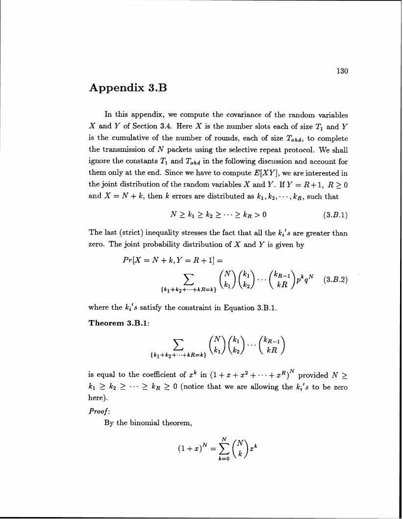
Appendix 3.B

In this appendix, we compute the covariance of the random variables

X and Y of Section 3.4. Here X is the number slots each of size TI and Y

is the cumulative of the number of rounds, each of size Tohd, to complete

the transmission of N packets using the selective repeat protocol. We shall

ignore the constants TI and Tohd in the following discussion and account for

them only at the end. Since we have to compute E[XY], we are interested in

the joint distribution of the random variables X and Y. If Y = R+ 1, R > 0

and X = N + k, then k errors are distributed as kl , k2, . - - , kR, such that

The last (strict) inequality stresses the fact that all the k i t s are greater than

zero. The joint probability distribution of X and Y is given by

where the kits satisfy the constraint in Equation 3.B.1.

Theorem 3.B.1:

is equal to the coefficient of x k in (1 + x + x 2 + . . . + xRIN provided N 2 k1 2 k2 2 - . - 2 kR 2 0 (notice that we are allowing the k i t s to be zero

here).

Pro0 f: By the binomial theorem,

Substituting xl (1 + x2) for x in the above equation, we get

and putting x1 = x2 = x we have

The left hand side of Equation 3.B.4 equals (1 + x + z21N. Continuing this

way, we can expand x2 in Equation 3.B .3 to x2 (1 + x3) and so on. This

proves the theorem. I

In the above derivation, we have allowed the ki's to be zero. This gives

us PT[X = N + k , Y 5 R+1]. Let A ( N + k , R ) = PT[X = N + k , Y < R+1]

and P ( N + k , R ) = PT[X = N + k , Y = R+1] . Then

Now,

If we denote the coefficient of xk in Equation B.6 as C(k, R), then

k N A(N + k, R) = C(k, R)p q (3.B.7)

Equations 3.B.5 and 3.B.7 finally give the probability of exactly R + 1 rounds

and k errors. Now we can compute

The covariance of X and Y is given by

E[X] and E[Y] have already been computed in Section 3.4. Equation 3.B.8

can be simplified as follows. Let Q(XY, z, R) be defined as:

- - zN [(1 - ( P Z ) ~ ' ' ) ~ - (1 - ( p ~ ) R ) N ] ( 3 . ~ . l ~ )

(1 - pzlN

On the other hand, from the definition of P ( N + E , R), and from equations

3.B.7, 3.B.8 and 3.B.10 we can see by inspection that

Using Equation 3.B.10, the inner sum on the right hand side becomes

Applying the formula for summation by parts to this expression, we get

Thus Equation 3.B.11 simplifies to

The first term in Equation 3.B.12 can be seen from Section 3.4 to be equal

to E [ X ] E [ Y ] . Hence, from equations 3.B.12 and 3.B.9, we have

For N p << 1, we can approximate this as

and finally, putting q = 1 - p we get

Recall that the right hand side has to be multiplied by TITohd to finally give

the correct covariance. In the range of interest, cov(X, Y) z NpTITohd for

small Np.

Appendix 5.A

We are interested in the variance of the time to absorption for a Con-

tinuous Time Markov Process, which starts off in a designated state i. Let

Ri = the time to absorption given we are in state i

t i = sojourn time in state i Hi(s) = Laplace transform of t i Fi(s) = Laplace transform of R; B = set of non-absorbing states

pij = Probability of going from st ate i to j in one step in the correspond-

ing discrete chain.

Then, by the Markov property

Taking the natural logarithm of both sides, we have

Differentiating equation 5.A.2 and setting s = 0, we get,

E[Q] = E[ti] + C pijE[Rj] (5.A.3) j€B- i

Differentiating equation 5.A.2 a second time, setting s = 0, we get, after

some algebra:

Var(Ri) = Var(Ti)+ C pijVar(j) j€B- i

which is the desired solution for the variance.

We also note that if io is the initial state, then EIRio] gives the expected

time to absorption for the Markov process of interest. This can be readily

generalized if the initial distribution of the initial states are available.