Analysis of Epistasis Correlation on NK Landscapes …medal-lab.org/files/2011002.pdfAnalysis of...

Analysis of Epistasis Correlation on NK Landscapes with Nearest-Neighbor Interac-tions

Martin Pelikan

MEDAL Report No. 2011002

February 2011

Abstract

Epistasis correlation is a measure that estimates the strength of interactions between problem variables. This

paper presents an empirical study of epistasis correlation on a large number of random problem instances of NK

landscapes with nearest neighbor interactions. The results are analyzed with respect to the performance of hybrid

variants of two evolutionary algorithms: (1) the genetic algorithm with uniform crossover and (2) the hierarchical

Bayesian optimization algorithm.

Keywords

Epistasis, epistasis correlation, problem difficulty, NK landscapes, genetic algorithms, estimation of distribution

algorithms, linkage learning.

Missouri Estimation of Distribution Algorithms Laboratory (MEDAL)

Department of Mathematics and Computer Science

University of Missouri–St. Louis

One University Blvd., St. Louis, MO 63121

E-mail: [email protected]

WWW: http://medal.cs.umsl.edu/

Analysis of Epistasis Correlation on NK Landscapes with

Nearest-Neighbor Interactions

Martin Pelikan

Missouri Estimation of Distribution Algorithms Laboratory (MEDAL)Dept. of Math and Computer Science, 320 CCB

University of Missouri in St. LouisOne University Blvd., St. Louis, MO 63121

[email protected]

February 9, 2011

Abstract

Epistasis correlation is a measure that estimates the strength of interactions between problemvariables. This paper presents an empirical study of epistasis correlation on a large number ofrandom problem instances of NK landscapes with nearest neighbor interactions. The resultsare analyzed with respect to the performance of hybrid variants of two evolutionary algorithms:(1) the genetic algorithm with uniform crossover and (2) the hierarchical Bayesian optimizationalgorithm.

Keywords: Epistasis, epistasis correlation, problem difficulty, NK landscapes, genetic algorithms,estimation of distribution algorithms, linkage learning.

1 Introduction

It has long been recognized that optimization problems with strong interactions between problemvariables are often more difficult for genetic and evolutionary algorithms (GEAs) than problemswhere variables are nearly independent (Goldberg, 1989; Davidor, 1990; Deb & Goldberg, 1991;Thierens, 1999; Pelikan, 2010). The strength of interactions between problem variables is oftenreferred to as epistasis, a term used in biology to denote the amount of interaction between differentgenes. A number of approaches have been developed to adapt operators of GEAs to tackle problemswith strong epistasis; these include for example linkage learning genetic algorithms (ping Chen, Yu,Sastry, & Goldberg, 2007; Harik & Goldberg, 1996) and estimation of distribution algorithms(EDAs) (Larranaga & Lozano, 2002; Pelikan, Goldberg, & Lobo, 2002; Lozano, Larranaga, Inza,& Bengoetxea, 2006; Pelikan, Sastry, & Cantu-Paz, 2006).

Two direct approaches were developed to measure the amount of epistasis in an optimizationproblem or the absence of it: (1) epistasis variance (Davidor, 1990) and (2) epistasis correlation (Ro-chet, Venturini, Slimane, & Kharoubi, 1998). Epistasis correlation is often considered more useful,because its range is [0, 1] and it is invariant with respect to linear transformations of fitness; theresults may thus often be easier to interpret and compare. Because epistasis is strongly relatedto problem difficulty, measuring epistasis should provide insight into the difficulty of a problem.Nonetheless, it has been also recognized that a problem with strong epistasis is not necessarilymore difficult than a problem with weaker epistasis (Rochet, Venturini, Slimane, & Kharoubi,

1

1998; Naudts & Kallel, 1998). Although there are numerous papers discussing epistasis and mea-sures of epistasis in the context of genetic and evolutionary algorithms (Davidor, 1990; Davidor,1991; Reeves & Wright, 1995; Rochet, Venturini, Slimane, & Kharoubi, 1998; Naudts & Kallel,1998), in most of these studies only a handful of problems are considered.

This paper presents a detailed empirical study of the relationship between problem parameters,the epistasis correlation, and the performance of two qualitatively different hybrid evolutionaryalgorithms, the genetic algorithm with uniform crossover (GA) (Holland, 1975; Goldberg, 1989;Syswerda, 1989), and the hierarchical Bayesian optimization algorithm (hBOA) (Pelikan, 2005).In GA with uniform crossover, variation operators do not take into account correlations betweenvariables and treat all variables as independent. On the other hand, hBOA can learn linkage; it isable to identify and exploit interactions between problem variables. Both GA and hBOA use hillclimbing based on the single-bit neighborhood to speed up convergence and reduce computationalrequirements. As the target class of problems, the paper considers NK landscapes with nearest-neighbor interactions (Pelikan, 2010). This problem class was chosen mainly because it providesa straightforward mechanism for tuning problem difficulty and level of epistasis, and it allowsgeneration of a large number of random problem instances with known optima.

The paper is organized as follows. Section 2 describes epistasis variance and epistasis correlation,which are the two primary direct measures of epistasis in optimization. Section 3 describes thealgorithms GA and hBOA, and the class of NK landscapes with nearest-neighbor interactions.Section 4 presents and discusses the experiments. Finally, section 5 summarizes and concludes thepaper.

2 Epistasis

For success in both applied and theoretical research in evolutionary computation it is importantto understand what makes one problem more difficult than another. Several approaches havebeen proposed to measure problem difficulty for evolutionary algorithms and other metaheuristics.The most popular measures include the fitness distance correlation (Jones & Forrest, 1995), theautocorrelation function (Weinberger, 1990), the epistasis correlation (Rochet, Venturini, Slimane,& Kharoubi, 1998), the signal-to-noise ratio (Goldberg, Deb, & Clark, 1992), and scaling (Thierens,Goldberg, & Pereira, 1998). While many of these measures are related to epistasis, this paperfocuses on approaches that measure epistasis directly.

In the remainder of this paper, candidate solutions are represented by binary strings of fixedlength n > 0, although many of the discussed concepts and methods can be extended to otheralphabets in a straightforward manner.

2.1 Epistasis Variance

This section describes epistasis variance, which is a measure of epistasis proposed by Davidor(1990) and is defined as the Euclidean distance between the linear approximation of the fitnessfunction and the actual fitness function over the population of all admissible solutions. To makethe computation of epistasis variance tractable for moderate to large string length, we reduce thecomputation of the epistasis variance to an arbitrary population of candidate solutions.

Assume a population P of N candidate solutions represented by n-bit binary strings. The

2

average fitness of solutions in P is defined as

f(P ) =1

N

∑

x∈P

f(x).

Let us define the set of solutions in P with the value vi in ith position as Pi(vi) and their numberby Ni(vi). Then, for each position i in a solution string, we may define the fitness contribution ofa bit vi as

fi(vi) =1

Ni(vi)

∑

x∈Pi(vi)

f(x) − f(P ) (1)

The linear approximation of f (Davidor, 1990; Reeves & Wright, 1995; Naudts, Suys, & Verschoren,1997; Rochet, Slimane, & Venturini, 1996) is defined as

flin(X1, X2, . . . , Xn) =n

∑

i=1

fi(Xi) + f(P ). (2)

It is of note that the above linear fitness approximation has also been used in the first approachto modeling the fitness function in estimation of distribution algorithms (Sastry, Goldberg, &Pelikan, 2001). The epistasis variance of f for population P is then defined as (Davidor, 1990;Davidor, 1991)

ξP (f) =

√

1

N

∑

x∈P

(f(x) − flin(x))2 (3)

One of the problems with epistasis variance is that its value changes even when the fitnessfunction is just multiplied by a constant. That is why several researchers have proposed to normalizethe epistasis variance, for example by dividing it by the variance of the fitness function (Manela &Campbell, 1992), or by using a normalized fitness function (Naudts, Suys, & Verschoren, 1997).

2.2 Epistasis Correlation

Epistasis correlation was proposed by Rochet, Venturini, Slimane, and Kharoubi (1998) as a mea-sure of epistasis that is invariant with respect to linear transformation of the fitness function (notonly multiplication by a constant). Let us define the sum of square differences between f and f(P )over all members of P as

sP (f) =∑

x∈P

(

f(x) − f(P ))2

.

Analogously, we may define the sum of square differences between flin and its average over P as

sP (flin) =∑

x∈P

(

flin(x) − flin(P ))2

where

flin(P ) =1

N

∑

x∈P

flin(x).

The epistasis correlation for the population P is then defined as

epicP (f) =

∑

x∈P

(

f(x) − f(P )) (

flin(x) − flin(P ))

√

sP (f)sP (flin)(4)

3

The main advantage of epistasis correlation is that it is invariant with respect to linear trans-formations of fitness and its range is [0, 1]. Consequently, epistasis correlation is much easier tointerpret than epistasis variance. These are the reasons why we use epistasis correlation in theremainder of this paper as the measure of epistasis.

2.3 Epistasis Measures and Difficulty

One of the problems with the epistasis correlation and the epistasis variance is that while the goal ofthese measures is to evaluate problem difficulty, the gap between problem difficulty and the epistasismeasures is quite substantial. For example, if the epistasis correlation is 1, then we know that theproblem is linear and it should thus be relatively easy to solve with practically any optimizationmethod. Nonetheless, as the epistasis correlation decreases, this measure alone cannot be used as asingle input to estimate problem difficulty because problem difficulty does not depend only on thepresence of epistasis but also on its character. This observation was pointed out in many studiesthat discussed the epistasis variance or the epistasis correlation, for example in Rochet, Venturini,Slimane, and Kharoubi (1998) and Naudts and Kallel (1998).

The weakness of the connection between problem difficulty and the measures of epistasis has ledto other models of problem difficulty originating in interactions between problem variables, such asdeception (Goldberg, 1989; Goldberg, 2002) and fluctuating crosstalk (Sastry, Pelikan, & Goldberg,2006; Goldberg, 2002). One of the difficulties with these models is that it is not straightforward toquantify them in practice.

Nonetheless, it is of note that the weakness of the connection between the epistasis measuresand problem difficulty is most often discussed on artificial problems that have little to do withthe real world and that were created just for the purpose of pointing out drawbacks of epistasismeasures. In this paper, we aim to analyze the epistasis measures and their relationship to problemdifficulty on a broad class of structured random problems, including both the easy and the difficultinstances.

2.4 Approximating Epistasis Correlation

Calculating the exact value of the epistasis correlation using a population of all possible stringsis intractable for moderate to large values of n. Furthermore, approximating the value of epista-sis correlation turns out to be slightly more challenging than approximating the values of someother measures of problem difficulty, such as the fitness distance correlation and the correlationlength (Pelikan, 2010). Since in this paper we considered 250,000 problem instances for which wecomputed the value of epistasis correlation, it was crucial ensure that the computation of epistasiscorrelation is computationally efficient. Of course, for the results to be useful, accuracy was justas important as efficiency.

To estimate the value of the epistasis analysis, we started with nexp = 10 independent experi-ments. In each of these experiments, we generated a population of 106 solutions, and we computedthe exact value of the epistasis correlation for the generated population. The resulting epistasiscorrelation values were averaged to compute the final estimate of the epistasis correlation. If theresults of the individual experiments indicated that the error in the average epistasis correlationvalue is away from its target value by more than 0.1% (assuming the normal distribution of theresults), another 10 experiments were executed. Regardless of the error, the maximum number ofexperiments was 1,000. That means that the resulting estimate was computed from 107 to 109

independently generated samples.

4

3 Problems and Methods

This section outlines the algorithms and fitness functions used in the experiments.

3.1 Algorithms

3.1.1 Genetic algorithm

The genetic algorithm (GA) (Holland, 1975; Goldberg, 1989) evolves a population of candidatesolutions typically represented by binary strings of fixed length. The initial population is generatedat random according to the uniform distribution over all binary strings. Each iteration startsby selecting promising solutions from the current population; we use binary tournament selectionwithout replacement. New solutions are created by applying variation operators to the populationof selected solutions. Specifically, crossover is used to exchange bits and pieces between pairs ofcandidate solutions and mutation is used to perturb the resulting solutions. Here we use uniformcrossover (Syswerda, 1989), and bit-flip mutation (Goldberg, 1989). To maintain useful diversityin the population, the new candidate solutions are incorporated into the original population usingrestricted tournament selection (RTS) (Harik, 1995). The run is terminated when terminationcriteria are met. In this paper, each run is terminated either when the global optimum has beenfound or when a maximum number of iterations has been reached.

3.1.2 Hierarchical BOA

The hierarchical Bayesian optimization algorithm (hBOA) (Pelikan & Goldberg, 2001; Pelikan &Goldberg, 2003; Pelikan, 2005) is an estimation of distribution algorithm (EDA) (Baluja, 1994;Muhlenbein & Paaß, 1996; Larranaga & Lozano, 2002; Pelikan, Goldberg, & Lobo, 2002; Lozano,Larranaga, Inza, & Bengoetxea, 2006; Pelikan, Sastry, & Cantu-Paz, 2006). EDAs—also calledprobabilistic model-building genetic algorithms (PMBGAs) (Pelikan, Goldberg, & Lobo, 2002)and iterated density estimation algorithms (IDEAs) (Bosman & Thierens, 2000)—differ from GAsby replacing standard variation operators of GAs such as crossover and mutation by building aprobabilistic model of promising solutions and sampling the built model to generate new candidatesolutions. The only difference between GA and hBOA variants used in this study is that instead ofusing crossover and mutation to create new candidate solutions, hBOA learns a Bayesian networkwith local structures (Chickering, Heckerman, & Meek, 1997; Friedman & Goldszmidt, 1999) as amodel of the selected solutions and generates new candidate solutions from the distribution encodedby this model. For more details on hBOA, see Pelikan and Goldberg (2001) and Pelikan (2005).

It is important to note that by building and sampling Bayesian networks, hBOA is able toscalably solve even problems with high levels of epistasis, assuming that the order of subproblemsin an adequate problem decomposition is upper bounded by a constant (Pelikan, Sastry, & Goldberg,2002). Since the variation operators of the GA variant studied here assume that the string positionsare independent whereas hBOA has a mechanism to deal with epistasis, it should be interestingto look at the effects of epistasis on these two algorithms. This is in fact the main reason for thechoice of these two algorithms. In this context, an EDA based on univariate models may have beenan even better choice than the GA with uniform crossover, but in that case most NK landscapesof larger size became intractable.

5

3.1.3 Bit-flip hill climber

The deterministic hill climber (DHC) is incorporated into both GA and hBOA to improve theirperformance similarly as in previous studies on using GA and hBOA for solving NK landscapesand related problems (Pelikan, Sastry, Goldberg, Butz, & Hauschild, 2009; Pelikan, 2010). DHCtakes a candidate solution represented by an n-bit binary string on input. Then, it performs one-bit changes on the solution that lead to the maximum improvement of solution quality. DHC isterminated when no single-bit flip improves solution quality and the solution is thus locally optimal.Here, DHC is used to improve every solution in the population before the evaluation is performed.

3.2 Nearest-neighbor NK landscapes

NK fitness landscapes (Kauffman, 1989) were introduced by Kauffman as tunable models of ruggedfitness landscape. An NK fitness landscape is fully defined by the following components: (1) Thenumber of bits, n, (2) the number of neighbors per bit, k, (3) a set of k neighbors Π(Xi) for the i-thbit for every i ∈ {1, . . . , n}, and (4) a subfunction fi defining a real value for each combination ofvalues of Xi and Π(Xi) for every i ∈ {1, . . . , n}. Typically, each subfunction is defined as a lookuptable. The objective function fnk to maximize is defined as

fnk(X1, X2, . . . , Xn) =n

∑

i=1

fi(Xi, Π(Xi)).

In this paper, we consider nearest-neighbor NK landscapes, in which neighbors of each bitare restricted to the k bits that immediately follow this bit. The neighborhoods wrap around;thus, for bits that do not have k bits to the right, the neighborhood is completed with the firstfew bits of solution strings. The reason for restricting neighborhoods to nearest neighbors wasto ensure that the problem instances can be solved in polynomial time even for k > 1 usingdynamic programming (Pelikan, 2010). The subfunctions are represented by look-up tables (aunique value is used for each instance of a bit and its neighbors), and each entry in the look-uptable is generated with the uniform distribution from [0, 1). To make the problem more difficult forconventional variation operators based on tight linkage between bits located close to each other,the string positions are randomly shuffled prior to optimization. The used class of NK landscapeswith nearest neighbors is thus the same as that in Pelikan (2010).

In this paper, we consider k ∈ {2, 3, 4, 5, 6} and n = 20 to 100 with step 10 (for scalabilityexperiments) or 20 (for epistasis correlation). For each combination of n and k, we generated andtested 10,000 unique problem instances. The reason for using such a large number of instances wasto get a sufficient number of samples for the various tests presented here. For GA, the results forinstances with n = 100 and k = 6 were too computationally expensive and they were thus omitted.In summary, for epistasis correlation, 250,000 independently generated problem instances were usedand 450,000 independently generated instances were used for experiments on scalability of hBOAand GA.

The difficulty of optimizing NK landscapes depends on all components defining an NK probleminstance (Wright, Thompson, & Zhang, 2000). Although NK landscapes with nearest neighborinteractions are polynomially solvable in terms of n (Pelikan, 2010), the difficulty of problem in-stances from this class generally increases as n and k grow. On nearest-neighbor NK landscapes,the time complexity of most evolutionary algorithms is expected to grow at least polynomially fastwith n, and no better than exponentially fast with k (Pelikan, Sastry, Goldberg, Butz, & Hauschild,2009; Pelikan, 2010).

6

20 40 60 80 100

102

103

104

Number of bits, n

Num

ber

of e

valu

atio

ns

k=6k=5k=4k=3k=2

20 40 60 80 10010

2

103

104

105

Number of bits, n

Num

ber

of D

HC

flip

s

k=6k=5k=4k=3k=2

2 3 4 5 610

3

104

105

Number of neighbors, k

Num

. of f

lips

or e

valu

atio

ns

Number of DHC flipsNumber of evaluations

(a) hBOA with local search.

20 40 60 80 100

102

103

104

Number of bits, n

Num

ber

of e

valu

atio

ns

k=6k=5k=4k=3k=2

20 40 60 80 10010

2

103

104

105

Number of bits, n

Num

ber

of D

HC

flip

s

k=6k=5k=4k=3k=2

2 3 4 5

103

104

105


Num

. of f

lips

or e

valu

atio

ns

Number of DHC flipsNumber of evaluations

(b) GA with uniform crossover and local search.

Figure 1: Performance of hBOA and GA with uniform crossover on nearest-neighbor NK landscapesof k = 2 to k = 6 and n = 20 to n = 100.

4 Experiments

4.1 hBOA and GA Parameter Settings

In hBOA, Bayesian networks with decision trees (Friedman & Yakhini, 1996; Chickering, Heck-erman, & Meek, 1997) are used as probabilistic models. To guide model building, the Bayesian-Dirichlet metric with likelihood equivalence (Chickering, Heckerman, & Meek, 1997) and the penaltyfor model complexity (Pelikan, 2005) is used. In GA, uniform crossover and bit-flip mutation areused as variation operators. The probability of crossover is pc = 0.6 and the probability of flippinga bit with mutation is 1/n where n is the number of bits. To select promising solutions, binarytournament selection without replacement is used in both GA and hBOA. New solutions are incor-porated into the original population using RTS (Harik, 1995) with window size w = min{n, N/20}as suggested by Pelikan (2005). The population sizes are identified using bisection (Sastry, 2001;Pelikan, 2005) to ensure convergence in 10 out of 10 independent runs. Each run is terminatedeither when the global optimum is found (success) or when the maximum number of iterationsequal to the number of bits n has been reached (failure).

4.2 Performance of hBOA and GA

Before presenting the results for the epistasis correlation, let us examine performance of hBOA andGA hybrids with respect to the values of n and k. Figure 1 shows the growth of the number ofevaluations and the number of local search steps (DHC flips) with n and k for both hybrids. Theresults confirm that the number of evaluations and the number of flips grow polynomially fast withthe number n of bits. The results also confirm that both these statistics grow at least exponentiallyfast with k.

7

103

104

1050.1

0.2

0.3

0.4

0.5

0.6

0.7

0.8

0.9

6

5

4

3

2

Number of evaluations for hBOA+DHC

Epi

stas

is c

orre

latio

n

k=2k=3k=4k=5k=6

103

104

105

1060.1

0.2

0.3

0.4

0.5

0.6

0.7

0.8

0.9

6

5

4

3

2

Number of DHC flips for hBOA+DHC

Epi

stas

is c

orre

latio

n

k=2k=3k=4k=5k=6

(a) Results for hBOA+DHC.

102

103

104

1050.1

0.2

0.3

0.4

0.5

0.6

0.7

0.8

0.9

5

4

3

2

Number of evaluations for GA+DHC

Epi

stas

is

k=2k=3k=4k=5

103

104

105

1060.1

0.2

0.3

0.4

0.5

0.6

0.7

0.8

0.9

5

4

3

2

Number of DHC flips for GA+DHC

Epi

stas

is

k=2k=3k=4k=5

(b) Results for GA+DHC.

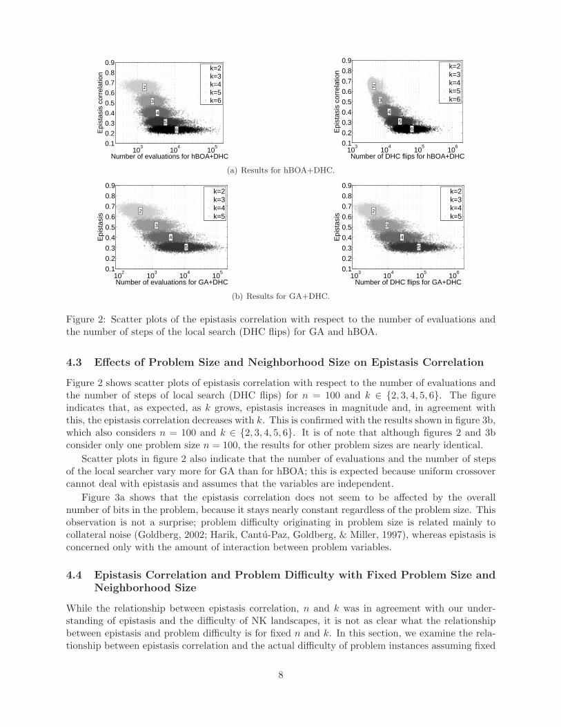
Figure 2: Scatter plots of the epistasis correlation with respect to the number of evaluations andthe number of steps of the local search (DHC flips) for GA and hBOA.

4.3 Effects of Problem Size and Neighborhood Size on Epistasis Correlation

Figure 2 shows scatter plots of epistasis correlation with respect to the number of evaluations andthe number of steps of local search (DHC flips) for n = 100 and k ∈ {2, 3, 4, 5, 6}. The figureindicates that, as expected, as k grows, epistasis increases in magnitude and, in agreement withthis, the epistasis correlation decreases with k. This is confirmed with the results shown in figure 3b,which also considers n = 100 and k ∈ {2, 3, 4, 5, 6}. It is of note that although figures 2 and 3bconsider only one problem size n = 100, the results for other problem sizes are nearly identical.

Scatter plots in figure 2 also indicate that the number of evaluations and the number of stepsof the local searcher vary more for GA than for hBOA; this is expected because uniform crossovercannot deal with epistasis and assumes that the variables are independent.

Figure 3a shows that the epistasis correlation does not seem to be affected by the overallnumber of bits in the problem, because it stays nearly constant regardless of the problem size. Thisobservation is not a surprise; problem difficulty originating in problem size is related mainly tocollateral noise (Goldberg, 2002; Harik, Cantu-Paz, Goldberg, & Miller, 1997), whereas epistasis isconcerned only with the amount of interaction between problem variables.

4.4 Epistasis Correlation and Problem Difficulty with Fixed Problem Size and

Neighborhood Size

While the relationship between epistasis correlation, n and k was in agreement with our under-standing of epistasis and the difficulty of NK landscapes, it is not as clear what the relationshipbetween epistasis and problem difficulty is for fixed n and k. In this section, we examine the rela-tionship between epistasis correlation and the actual difficulty of problem instances assuming fixed

8

20 40 60 80 100 1200

0.10.20.30.40.50.60.70.80.9

1

Number of bits, n

Epi

stas

is c

orre

latio

n

k=2k=3k=4k=5k=6

(a) Epistasis correlation with re-spect to n.

2 3 4 5 60

0.10.20.30.40.50.60.70.80.9

1


Epi

stas

is c

orre

latio

n

Avg. epistasis corr., n=100

(b) Epistasis correlation with re-spect to k.

Figure 3: Epistasis correlation with respect to the number n of bits and the number k of neighborsof nearest-neighbor NK landscapes.

n and k.

Specifically, for various combinations of n and k, several subsets of easy and difficult probleminstances are selected, and for each of these subsets, the average number of steps of local search andthe average epistasis correlation are presented. As subsets, we select the 10%, 25% and 50% easiestinstances, the 10%, 25% and 50% hardest instances, and all instances for the specific combinationof n and k regardless of their difficulty. Since for each combination of n and k, 10,000 instanceswere used, even the smallest subset of 10% instances contains 1,000 instances. The difficulty of aninstance is measured by the actual number of steps of local search using the optimization methodunder consideration (either GA with uniform crossover and DHC, or hBOA with DHC). In mostcases, n = 100 and k ∈ {2, 3, 4, 5, 6}. The results for other problem sizes are similar. However, forGA with uniform crossover, resource constraints did not allow us to complete experiments k = 6and n = 90 or n = 100, so we used n = 80 for k = 6. The results are shown in tables 1 and 2.

As shown in table 1, for hBOA with DHC and most values of k, the values of epistasis correlationare in agreement with the actual difficulty of the subsets of instances. This is in agreement with ourintuition that as the problem difficulty increases, the epistasis correlation decreases, indicating anincreased level of epistasis. Nonetheless, as k grows, the differences between the values of epistasiscorrelation for the different subsets of instances decrease. In fact, for k = 5 and k = 6, the values ofepistasis correlation sometimes increase with problem difficulty. While these results are somewhatsurprising, they can be explained by the fact that hBOA is able to deal with problems with epistasisof bounded order efficiently. That is why hBOA should not be as sensitive to epistasis as manyother evolutionary algorithms.

As shown in table 2, for GA with uniform crossover and DHC, the values of epistasis correlationare also in agreement with our understanding of how epistasis affects problem difficulty. Specifically,as the problem instances become more difficult, the epistasis correlation decreases, indicating anincreased level of epistasis. In fact, for GA, the results are in agreement with our understandingof epistasis and problem difficulty even for larger values of k, although the differences between thevalues of epistasis in different subsets decrease with k.

The differences between the results for hBOA and GA confirm that the effect of epistasis shouldbe weaker for hBOA than for GA because hBOA can deal with epistasis better than conventionalGAs by detecting and using interactions between problem variables. The differences are certainlysmall, but so are the differences between the epistasis correlation values between the subsets ofproblems that are even orders of magnitude different in terms of the computational time. Thedifferences between a conventional GA with no linkage learning and one of the most advanced

9

EDAs are among the most interesting results in this paper.

5 Summary and Conclusions

This paper discussed epistasis and its relationship with problem difficulty. To measure epistasis,epistasis correlation was used. The empirical analysis considered hybrids of two qualitatively dif-ferent evolutionary algorithms and a large number of instances of nearest-neighbor NK landscapes.

The use of epistasis correlation in assessing problem difficulty has received a lot of criti-cism (Naudts, Suys, & Verschoren, 1997; Rochet, Venturini, Slimane, & Kharoubi, 1998). Themain reason for this is that although the absence of epistasis does imply that a problem is easy, thepresence of epistasis does not necessarily imply that the problem is difficult. Nonetheless, given ourcurrent understanding of problem difficulty, there is no doubt that introducing epistasis increasesthe potential of a problem to be difficult.

This paper indicated that for randomly generated NK landscapes with nearest-neighbor inter-actions, epistasis correlation correctly captures the fact that the problem instances become moredifficult as the order of interactions (number of neighbors) increases. Additionally, the resultsconfirmed that for a fixed problem size and order of interactions, sets of more difficult probleminstances have lower values of epistasis correlation (and, thus, stronger epistasis). The results in-dicated also that evolutionary algorithms capable of linkage learning are less sensitive to epistasisthan conventional evolutionary algorithms.

The bad news is that the results confirmed that epistasis correlation does not provide a singleinput for the practitioner to assess problem difficulty, even if we assume that the problem size andthe order of interactions are fixed, and all instances are generated from the same distribution. Inmany cases, simple problems included strong epistasis and hard problems included weak epistasis.A similar observation has been made by Pelikan (2010) for the correlation length and the fitnessdistance correlation. However, compared to these other popular measures of problem difficulty,epistasis correlation belongs to one of the more accurate ones, at least for the class of randomlygenerated NK landscapes with nearest-neighbor interactions.

One of the important topics of future work would be to compile some of the past results inanalysis of various measures of problem difficulty with the results presented here, and explore theways in which different measures of problem difficulty can be combined to provide the practitionera better indication of what problem instances are more difficult and what problem instances areeasier. The experimental study presented in this paper should also be extended to other classesof problems, especially those that allow one to generate a large set of random problem instances.Classes of spin glass optimization problems and graph problems are good candidates for theseefforts.

Acknowledgments

This project was sponsored by the National Science Foundation under CAREER grant ECS-0547013, and by the Univ. of Missouri in St. Louis through the High Performance ComputingCollaboratory sponsored by Information Technology Services. Most experiments were performedon the Beowulf cluster maintained by ITS at the Univ. of Missouri in St. Louis. Any opinions,findings, and conclusions or recommendations expressed in this material are those of the authorsand do not necessarily reflect the views of the National Science Foundation.

10

References

Baluja, S. (1994). Population-based incremental learning: A method for integrating genetic searchbased function optimization and competitive learning (Tech. Rep. No. CMU-CS-94-163). Pitts-burgh, PA: Carnegie Mellon University.

Bosman, P. A. N., & Thierens, D. (2000). Continuous iterated density estimation evolutionaryalgorithms within the IDEA framework. Workshop Proc. of the Genetic and Evol. Comp.Conf. (GECCO-2000), 197–200.

Chickering, D. M., Heckerman, D., & Meek, C. (1997). A Bayesian approach to learning Bayesiannetworks with local structure (Technical Report MSR-TR-97-07). Redmond, WA: MicrosoftResearch.

Davidor, Y. (1990). Epistasis variance: Suitability of a representation to genetic algorithms.Complex Systems, 4 , 369–383.

Davidor, Y. (1991). Genetic algorithms and robotics: a heuristic strategy for optimization. Sin-gapore: World Scientific Publishing.

Deb, K., & Goldberg, D. E. (1991). Analyzing deception in trap functions (IlliGAL Report No.91009). Urbana, IL: University of Illinois at Urbana-Champaign, Illinois Genetic AlgorithmsLaboratory.

Friedman, N., & Goldszmidt, M. (1999). Learning Bayesian networks with local structure. InJordan, M. I. (Ed.), Graphical models (pp. 421–459). MIT Press.

Friedman, N., & Yakhini, Z. (1996). On the sample complexity of learning Bayesian networks.Proc. of the Conf. on Uncertainty in Artificial Intelligence (UAI-96), 274–282.

Goldberg, D. E. (1989). Genetic algorithms in search, optimization, and machine learning. Read-ing, MA: Addison-Wesley.

Goldberg, D. E. (2002). The design of innovation: Lessons from and for competent geneticalgorithms. Kluwer.

Goldberg, D. E., Deb, K., & Clark, J. H. (1992). Genetic algorithms, noise, and the sizing ofpopulations. Complex Systems, 6 , 333–362.

Harik, G. R. (1995). Finding multimodal solutions using restricted tournament selection. Proc.of the Int. Conf. on Genetic Algorithms (ICGA-95), 24–31.

Harik, G. R., Cantu-Paz, E., Goldberg, D. E., & Miller, B. L. (1997). The gambler’s ruin problem,genetic algorithms, and the sizing of populations. Proc. of the Int. Conf. on EvolutionaryComputation (ICEC-97), 7–12.

Harik, G. R., & Goldberg, D. E. (1996). Learning linkage. Foundations of Genetic Algorithms , 4 ,247–262.

Holland, J. H. (1975). Adaptation in natural and artificial systems. Ann Arbor, MI: Universityof Michigan Press.

Jones, T., & Forrest, S. (1995). Fitness distance correlation as a measure of problem difficultyfor genetic algorithms. Proc. of the Int. Conf. on Genetic Algorithms (ICGA-95), 184–192.

Kauffman, S. (1989). Adaptation on rugged fitness landscapes. In Stein, D. L. (Ed.), LectureNotes in the Sciences of Complexity (pp. 527–618). Addison Wesley.

Larranaga, P., & Lozano, J. A. (Eds.) (2002). Estimation of distribution algorithms: A new toolfor evolutionary computation. Boston, MA: Kluwer.

11

Lozano, J. A., Larranaga, P., Inza, I., & Bengoetxea, E. (Eds.) (2006). Towards a new evolution-ary computation: Advances on estimation of distribution algorithms. Springer.

Manela, M., & Campbell, J. A. (1992). Harmonic analysis, epistasis and genetic algorithms.Parallel Problem Solving from Nature, 59–66.

Muhlenbein, H., & Paaß, G. (1996). From recombination of genes to the estimation of distribu-tions I. Binary parameters. Parallel Problem Solving from Nature, 178–187.

Naudts, B., & Kallel, L. (1998). Some facts about so called GA-hardness measures (TechnicalReport 379). France: Ecole Polytechnique, CMAP.

Naudts, B., Suys, D., & Verschoren, A. (1997). Epistasis as a basic concept in formal landscapeanalysis. Proc. of the Int. Conf. on Genetic Alg. (ICGA-97), 65–72.

Pelikan, M. (2005). Hierarchical Bayesian optimization algorithm: Toward a new generation ofevolutionary algorithms. Springer.

Pelikan, M. (2010). NK landscapes, problem difficulty, and hybrid evolutionary algorithms. Ge-netic and Evol. Comp. Conf. (GECCO-2010), 665–672.

Pelikan, M., & Goldberg, D. E. (2001). Escaping hierarchical traps with competent geneticalgorithms. Genetic and Evol. Comp. Conf. (GECCO-2001), 511–518.

Pelikan, M., & Goldberg, D. E. (2003). A hierarchy machine: Learning to optimize from natureand humans. Complexity , 8 (5), 36–45.

Pelikan, M., Goldberg, D. E., & Lobo, F. (2002). A survey of optimization by building and usingprobabilistic models. Computational Optimization and Applications , 21 (1), 5–20.

Pelikan, M., Sastry, K., & Cantu-Paz, E. (Eds.) (2006). Scalable optimization via probabilisticmodeling: From algorithms to applications. Springer-Verlag.

Pelikan, M., Sastry, K., & Goldberg, D. E. (2002). Scalability of the Bayesian optimizationalgorithm. International Journal of Approximate Reasoning , 31 (3), 221–258.

Pelikan, M., Sastry, K., Goldberg, D. E., Butz, M. V., & Hauschild, M. (2009). Performanceof evolutionary algorithms on NK landscapes with nearest neighbor interactions and tunableoverlap. Genetic and Evol. Comp. Conf. (GECCO-2009), 851–858.

ping Chen, Y., Yu, T.-L., Sastry, K., & Goldberg, D. E. (2007). A survey of genetic link-age learning techniques (IlliGAL Report No. 2007014). Urbana, IL: University of Illinois atUrbana-Champaign, Illinois Genetic Algorithms Laboratory.

Reeves, C. R., & Wright, C. C. (1995). Epistasis in genetic algorithms: An experimental designperspective. Proceedings of the 6th International Conference on Genetic Algorithms , 217–224.

Rochet, S., Slimane, M., & Venturini, G. (1996). Epistasis for real encoding in genetic algorithms.In Proceedings of the Australian New Zealand Conference on Intelligent Information Systems,ANZIIS 96, Adelaide, South Australia, 18-20 November 1996 (pp. 268–271).

Rochet, S., Venturini, G., Slimane, M., & Kharoubi, E. M. E. (1998). A critical and empiricalstudy of epistasis measures for predicting ga performances: A summary. In Selected Papersfrom the Third European Conference on Artificial Evolution, AE ’97 (pp. 275–286). London,UK: Springer-Verlag.

Sastry, K. (2001). Evaluation-relaxation schemes for genetic and evolutionary algorithms. Mas-ter’s thesis, University of Illinois at Urbana-Champaign, Department of General Engineering,Urbana, IL.

12

Sastry, K., Goldberg, D. E., & Pelikan, M. (2001). Don’t evaluate, inherit. Genetic and Evol.Comp. Conf. (GECCO-2001), 551–558.

Sastry, K., Pelikan, M., & Goldberg, D. E. (2006). Efficiency enhancement of estimation of distri-bution algorithms. In Pelikan, M., Sastry, K., & Cantu-Paz, E. (Eds.), Scalable Optimizationvia Probabilistic Modeling: From Algorithms to Applications (pp. 161–185). Springer.

Syswerda, G. (1989). Uniform crossover in genetic algorithms. Proc. of the Int. Conf. on GeneticAlgorithms (ICGA-89), 2–9.

Thierens, D. (1999). Scalability problems of simple genetic algorithms. Evolutionary Computa-tion, 7 (4), 331–352.

Thierens, D., Goldberg, D. E., & Pereira, A. G. (1998). Domino convergence, drift, and thetemporal-salience structure of problems. Proc. of the Int. Conf. on Evolutionary Computation(ICEC-98), 535–540.

Weinberger, E. (1990). Correlated and uncorrelated fitness landscapes and how to tell the differ-ence. Biological Cybernetics, 63 (5), 325–336.

Wright, A. H., Thompson, R. K., & Zhang, J. (2000). The computational complexity of N-Kfitness functions. IEEE Trans. on Evolutionary Computation, 4 (4), 373–379.

13

hBOA, n = 100, k = 2:desc. of DHC steps until epistasisinstances optimum correlation10% easiest 3330.9 (163.9) 0.6645 (0.030)25% easiest 3550.2 (217.0) 0.6608 (0.030)50% easiest 3758.6 (265.2) 0.6580 (0.030)all instances 4436.2 (1019.5) 0.6534 (0.031)50% hardest 5113.8 (1044.2) 0.6487 (0.031)25% hardest 5805.5 (1089.4) 0.6466 (0.031)10% hardest 6767.6 (1152.3) 0.6447 (0.032)





Table 1: Epistasis correlation for easy and hardinstances for hBOA.

GA (uniform), n = 100, k = 2:desc. of DHC steps until epistasisinstances optimum correlation10% easiest 1493.1 (259.4) 0.6660 (0.028)25% easiest 1881.9 (373.9) 0.6625 (0.030)50% easiest 2332.3 (543.2) 0.6588 (0.030)all instances 3516.7 (1741.5) 0.6534 (0.031)50% hardest 4701.0 (1722.0) 0.6479 (0.031)25% hardest 5840.9 (1800.5) 0.6443 (0.031)10% hardest 7358.3 (2002.9) 0.6395 (0.030)





Table 2: Epistasis correlation for easy and hardinstances for GA.

14

Analysis of Epistasis Correlation on NK Landscapes …medal-lab.org/files/2011002.pdfAnalysis of...

Documents

Transcript of Analysis of Epistasis Correlation on NK Landscapes …medal-lab.org/files/2011002.pdfAnalysis of...