Analysis of Energy Efficient Curtain Wall Design ...
216
A thesis submitted to the Faculty of the Graduate School of the University of Colorado in partial fulfillment of the requirements for the degree of Master of Science Department of Civil, Environmental, and Architectural Engineering 2017 by Katherine M. DuMez © Mark Eekhoff Analysis of Energy Efficient Curtain Wall Design Considerations in Highrise Buildings
Transcript of Analysis of Energy Efficient Curtain Wall Design ...

A thesis submitted to the
Faculty of the Graduate School of the
University of Colorado in partial fulfillment
of the requirements for the degree of
Master of Science
Department of Civil, Environmental, and Architectural Engineering
2017
by Katherine M. DuMez
© Mark Eekhoff
Analysis of Energy Efficient Curtain Wall Design Considerations in Highrise Buildings

ii
This thesis entitled: Analysis of Energy Efficient Curtain Wall Design Considerations in Highrise Buildings
Written by Katherine M. DuMez Has been approved for the Department of Civil, Environmental, and Architectural Engineering
_____________________________________________ Prof. Z. John Zhai, Ph.D.
____________________________________________ Prof. Moncef Krarti, Ph.D., P.E.
_____________________________________________ Prof. C. Walter Beamer IV, Ph.D.
Date__________________________
The final copy of this thesis has been examined by the signatories and we find that both the content and the form meet acceptable presentation standards of scholarly work in the above mentioned
discipline.

Abstract
iii
Du Mez, Katherine M. (M.S., Department of Civil, Environmental, and Architectural Engineering)
Analysis of Energy Efficient Curtain Wall Design Considerations in Highrise Buildings
Thesis directed by Prof. Z. John Zhai, Ph.D.
Today’s built environment is responsible for 40% of the annual energy consumption in the
United States. There is great potential for improvements in building design to reduce the
contribution of the built environment to the national energy consumption. In order for widespread
change to take place, architects and engineers must be provided with the tools necessary to
understand the energy implications of their design decisions.
The iconic skyscrapers that form our nation’s skylines represent a large sector of buildings
that is in need of improvements in energy efficiency. The curtain wall façades in highrise buildings
provide a powerful aesthetic, but when not designed properly, the façade can be a major weakness
in terms of energy efficiency. A building energy model representative of a “typical” highrise building
within the U.S. was used to identify the potential weaknesses in the façade of a highrise building
and to characterize the general energy consumption of a highrise building design. The model was
then used to provide quantification for the energy consumption savings and annual energy cost
savings that can be achieved with an optimized curtain wall design.
Based upon the findings, a set of climate-specific recommendations were made that identify
the variables that have the most potential within a given climate to provide annual energy savings.
The ranges of values for each variable in the analysis were based on products currently on the
market. The results of this analysis present an argument for increased evaluation of the
performance characteristics of curtain walls in highrise buildings, and offer useful design guidance
to help architects and engineers to make informed decisions towards a more energy efficient
curtain wall and therefore building.

Acknowledgements
iv
Acknowledgements
I would like to thank the people that guided me and supported me through this
process. I thank Dr. Zhai for acting as my advisor throughout this process, for all the insight
and direction he provided. I would also like to thank my other committee members, Dr.
Krarti and Dr. Beamers for being willing to hear my ideas and offer their insight as well.
I would like to thank my employers at MKK Consulting Engineers for allowing me to
learn more about the commercial building design industry, for affording me the flexibility
to work and perform my research, and for supporting me through the process.
I owe a huge thanks to my friends and family who supported me and encouraged me
through the process, and to my fellow “Bat Cave” members for helping keep the sanity
intact. I hope that I am able to return the kindness and encouragement that was afforded
me by so many throughout this process.

Table of Contents
v
Table of Contents
Acknowledgements ............................................................................................................................................. iv
Table of Contents .................................................................................................................................................. v
Tables......................................................................................................................................................................... x
Figures ...................................................................................................................................................................... xi
Chapter 1: Introduction ...................................................................................................................................... 1
1.1 Introduction ..................................................................................................................................................... 1
Chapter 2: Literature Review ........................................................................................................................... 3
2.1 History of the Highrise Building .............................................................................................................. 3
2.2 Curtain Walls ................................................................................................................................................... 8
2.3 Glazing ............................................................................................................................................................. 12
2.3.1 Tinted Glazing ...................................................................................................................................... 13
2.3.2 Surface Coatings ................................................................................................................................. 15
2.3.3 Insulating Glass ................................................................................................................................... 18
2.3.4 Switchable Glazing ............................................................................................................................. 20
2.3.5 Directional Control ............................................................................................................................ 24
2.4 Shading ........................................................................................................................................................... 25
2.5 Double-Skin Façades ................................................................................................................................. 27
2.6 Thermal Concerns ...................................................................................................................................... 30
2.6.1 Thermal Bridging ............................................................................................................................... 30
2.6.2 Occupant Comfort .............................................................................................................................. 31
2.7 Ventilation and HVAC ................................................................................................................................ 35

Table of Contents
vi
2.7.1 HVAC loads and Energy Consumption ....................................................................................... 35
2.7.2 Natural Ventilation ............................................................................................................................ 38
2.8 Integrated Design Process ....................................................................................................................... 41
2.9 Code Compliance ......................................................................................................................................... 45
2.10 Case Studies ................................................................................................................................................ 48
2.10.1 Energy Efficient Highrise Retrofit: The Empire State Building ..................................... 48
2.10.2 Energy Efficient New Construction .......................................................................................... 50
2.11 Application .................................................................................................................................................. 51
Chapter 3: Highrise Building Energy Model ............................................................................................ 54
3.1 Building Energy Simulation Tool .......................................................................................................... 54
3.2 Department of Energy Benchmark Building .................................................................................... 55
3.3 Highrise Baseline Model .......................................................................................................................... 57
3.3.1 Highrise Geometry ............................................................................................................................. 57
3.2.2 Climate Zone Selection ..................................................................................................................... 59
3.2.2 Updated Baseline ................................................................................................................................ 60
Chapter 4: Comparison of Highrise Baseline Model ............................................................................. 61
4.1 DOE Benchmark Building updated to DOE Benchmark 32 Stories ......................................... 61
4.2 DOE Benchmark Building updated to Highrise Baseline ............................................................ 63
4.3 ASHRAE 90.1-2010 Highrise Baseline Models ................................................................................ 65
Chapter 5: Curtain Wall Envelope Analysis ............................................................................................. 69
5.1 Curtain Wall Variables .............................................................................................................................. 69
5.2 Opaque Envelope U-value ....................................................................................................................... 73

Table of Contents
vii
5.3 Window-to-Wall Ratio .............................................................................................................................. 76
5.4 Overhang Depth .......................................................................................................................................... 82
5.5 Window U-value .......................................................................................................................................... 86
5.6 Window Solar Heat Gain Coefficient ................................................................................................... 93
5.7 Impacts of Daylight Control .................................................................................................................... 99
5.7.1 Daylight Control and Window-to-wall Ratio ......................................................................... 100
5.7.2 Daylight Control and Overhang Depth ..................................................................................... 102
5.7.3 Daylight Control and Visible Transmittance ......................................................................... 103
Chapter 6: Parametric Analysis of Window Properties .................................................................... 106
6.1 Parametric Analysis of Window Properties ................................................................................... 106
6.1.1 Sensitivity Analysis .......................................................................................................................... 108
6.1.2 Energy Consumption Optimization ........................................................................................... 113
6.1.3 Energy Cost Optimization ............................................................................................................. 115
6.2 Impacts of Optimization ......................................................................................................................... 118
6.2.1 Equipment Sizing ............................................................................................................................. 118
6.2.2 Occupant Comfort ............................................................................................................................ 121
6.2.3 Aesthetic and View Quality ........................................................................................................... 123
Chapter 7: Results ............................................................................................................................................ 124
7.1 Design Recommendations ..................................................................................................................... 124
7.2 Summary and Future Work .................................................................................................................. 125
7.3 Conclusion ................................................................................................................................................... 127
References .......................................................................................................................................................... 128
Appendix A: Envelope Values ...................................................................................................................... 134

Table of Contents
viii
Appendix B: Window-to-Wall Ratio Results .......................................................................................... 137
Miami, FL WTW Ratio Results ................................................................................................................ 137
Houston, TX Results ................................................................................................................................... 138
Phoenix, AZ WTW Ratio Results ............................................................................................................ 139
Atlanta, GA WTW Ratio Results ............................................................................................................. 141
San Francisco, CA WTW Ratio Results ................................................................................................ 142
Baltimore, MD WTW Ratio Results ...................................................................................................... 143
Seattle, WA WTW Ratio Results ............................................................................................................ 145
Chicago, IL WTW Ratio Results .............................................................................................................. 146
Denver, CO WTW Ratio Results ............................................................................................................. 147
Helena, MT WTW Ratio Results ............................................................................................................. 149
Duluth, MN WTW Ratio Results ............................................................................................................. 150
Appendix C: Window U-values Results.................................................................................................... 152
Miami, FL Window U-value Results ..................................................................................................... 152
Houston, TX Window U-value Results ................................................................................................ 153
Phoenix, AZ Window U-value Results ................................................................................................. 154
Atlanta, GA Window U-value Results................................................................................................... 156
San Francisco, CA Window U-value Results...................................................................................... 157
Baltimore, MD Window U-value Results ............................................................................................ 158
Seattle, WA Window U-value Results .................................................................................................. 160
Chicago, IL Window U-value Results ................................................................................................... 161
Denver, CO Window U-value Results ................................................................................................... 162
Helena, MT Window U-value Results .................................................................................................. 164
Duluth, MN Window U-value Results .................................................................................................. 165
Appendix D: Solar Heat Gain Coefficient Analysis Results ............................................................... 167
Miami, FL SHGC Results ............................................................................................................................ 167
Houston, TX SHGC Results ....................................................................................................................... 168
Phoenix, AZ SHGC Results ........................................................................................................................ 169
San Francisco, CA SHGC Results ............................................................................................................ 171

Table of Contents
ix
Baltimore, MD SGHC Results ................................................................................................................... 172
Seattle, WA SHGC Results ......................................................................................................................... 174
Chicago, IL SHGC Results .......................................................................................................................... 175
Denver, CO SHGC Results ......................................................................................................................... 176
Helena, MT SHGC Results ......................................................................................................................... 178
Duluth, MN SHGC Results ......................................................................................................................... 179
Appendix E: Visible Transmittance Analysis Results ......................................................................... 181
Miami, FL Visible Transmittance Results ........................................................................................... 181
Houston, TX Visible Transmittance Results ...................................................................................... 181
Phoenix, AZ Visible Transmittance Results....................................................................................... 182
Atlanta, GA Visible Transmittance Results ........................................................................................ 183
San Francisco, CA Visible Transmittance Results ........................................................................... 183
Baltimore, MD Visible Transmittance Results ................................................................................. 184
Seattle, WA Visible Transmittance Results ....................................................................................... 185
Chicago, IL Visible Transmittance Results ........................................................................................ 185
Denver, CO Visible Transmittance Results ........................................................................................ 186
Helena, MT Visible Transmittance Results ........................................................................................ 187
Duluth, MN Visible Transmittance Results ....................................................................................... 187
Appendix F: Window Properties for Highest and Lowest Ten Energy Consumers................ 189

Tables
x
Tables
Table 1: Energy consumption comparison [15] ..................................................................................... 18
Table 2: DOE Benchmark Building variables and sources ................................................................. 56
Table 3: DOE Benchmark Building variables updated to Highrise Baseline ............................... 60
Table 4: Energy Use Intensity for 12 stories vs. 32 stories ............................................................... 62
Table 5: Energy Use Intensity for New Construction by Location .................................................. 65
Table 6: Simulated Variables and Ranges Used ..................................................................................... 71
Table 7: Sensitivity of Annual Energy Consumption and Annual Cost to WTW Ratio ............ 80
Table 8: Cost of Facade with Increased WTW Ratio ............................................................................. 81
Table 9: Simple Payback Period Calculation for Overhang Depth on All Façades - Miami and
Chicago ................................................................................................................................................................... 84
Table 10: Simple Payback Period Calculation for Overhang Depth on South and East
Facades – Miami and Chicago ........................................................................................................................ 85
Table 11: Sensitivity of Annual Energy Consumption and Annual Cost to Window U-value 90
Table 12: Estimated Simple Payback Period for Reducing U-value to 0.08 Btu/hr*ft2*°F .... 91
Table 13: Sensitivity of Annual Energy Consumption and Cost with respect to change in
SHGC ........................................................................................................................................................................ 95
Table 14: Estimated Simple Payback Period for Reducing SHGC.................................................... 96
Table 15: Window Properties for Parametric Analysis .................................................................... 107
Table 16: Maximum and Minimum Annual Energy Consumption and Associated Utility
Costs ...................................................................................................................................................................... 119

Figures
xi
Figures
Figure 1: Zoning Law of 1916 [5] ................................................................................................................... 4
Figure 2: Curtain Wall System Types [6] ..................................................................................................... 9
Figure 3: Left to right - Empire State Building, Chrysler Building, Swiss Re Headquarters,
Bank of China [7] ................................................................................................................................................ 11
Figure 4: Spectral transmittance of glazing materials [11] ............................................................... 13
Figure 5: Luminous efficacy of glazing materials [11]......................................................................... 14
Figure 6: Cooling and heating energy loads for (a) Mexico CIty and (b) Ottowa [14] ............ 17
Figure 7: Cross-section of a SAGE Electrochromic window [20] .................................................... 21
Figure 8: Comparison of energy consumption for shading and lighting control [34] ............. 26
Figure 9: Thermodynamics of a DSF [34] ................................................................................................. 28
Figure 10: Cross-section of one DSF strategy [5] .................................................................................. 29
Figure 11: PPD for cold and cloudy climate of Shillong [10] ............................................................. 32
Figure 12: PPD for hot and dry climate of Jodhpur [10] ..................................................................... 32
Figure 13: Natural ventilation in isolated spaces [55] ........................................................................ 40
Figure 14: Natural ventilation through an atrium [55] ....................................................................... 40
Figure 15: Tall Building System Integration Web [58] ....................................................................... 42
Figure 16: DOE Benchmark Building – Large Office Zoning Plan .................................................... 56
Figure 17: Height of highrise buildings in the United States [86] ................................................... 58
Figure 18: Number of floors in highrise buildings in the United States [86] .............................. 58
Figure 19: ASHRAE Climate Zone classifications and representative cities [84] ...................... 59
Figure 20: 3D image of Highrise Baseline................................................................................................. 61
Figure 21: Site Energy Savings through updates to ASHRAE 90.1-2010 ..................................... 63
Figure 22: Annual Sensible Heat Gain and Loss Components for Miami and Chicago ............ 66
Figure 23: Miami Annual End Use Energy ................................................................................................ 67
Figure 24: Chicago Annual End Use Energy ............................................................................................. 67
Figure 25: Miami Heating/Cooling Energy by Zone ............................................................................. 68
Figure 26: Chicago Heating/Cooling Energy by Zone .......................................................................... 68
Figure 27: Wall U-value - Annual Energy Consumption Difference from Baseline - Miami, FL
................................................................................................................................................................................... 73

Figures
xii
Figure 28: Wall U-value - Annual Energy Cost Difference from Baseline - Miami, FL ............. 74
Figure 29: Wall U-value - Annual Energy Consumption Difference from Baseline - Chicago,
IL ............................................................................................................................................................................... 74
Figure 30: Wall U-value - Annual Energy Cost Difference from Baseline - Chicago, IL ........... 74
Figure 31: Sensible Gains - Miami, FL ........................................................................................................ 76
Figure 32: Sensible Gains Percent Difference from Baseline - Miami, FL .................................... 76
Figure 33: Sensible Gains - Chicago, IL ...................................................................................................... 77
Figure 34: Sensible Gains Percent Difference from Baseline - Chicago, IL .................................. 77
Figure 35: Window-to-wall Ratio –Heating and Cooling Energy Difference from Baseline –
Miami, FL ............................................................................................................................................................... 78
Figure 36: Window-to-wall Ratio – Percent Heating and Cooling Energy Difference from
Baseline - Chicago, IL ........................................................................................................................................ 78
Figure 37: All Climates - Energy consumption vs. Window-to-wall Ratio ................................... 79
Figure 38: All Climates - Annual Energy Cost vs. Window-to-wall Ratio ..................................... 79
Figure 39: Overhang Depth - Energy Consumption Difference from Baseline - Miami, FL ... 82
Figure 40: Overhang Depth - Energy Cost Difference from Baseline - Miami, FL ..................... 82
Figure 41: Overhang Depth - Energy Consumption Difference from Baseline - Chicago, IL 83
Figure 42: Overhang Depth - Energy Cost Difference from Baseline - Chicago, IL ................... 83
Figure 43: Window U-value - Energy Consumption Change from Baseline – Miami, FL ....... 86
Figure 44: Window U-value – Percent Cooling Energy Savings from Baseline – Miami, FL . 87
Figure 45: Energy Consumption Change from Baseline - Chicago, IL ........................................... 88
Figure 46: U-value – Percent Heating and Cooling Energy Savings from Baseline - Chicago,
IL ............................................................................................................................................................................... 88
Figure 47: Window U-value - Cost Difference from Baseline - Miami, FL .................................... 89
Figure 48: Window U-value - Cost Difference from Baseline - Chicago, IL .................................. 89
Figure 49: SHGC - Energy Consumption Difference from Baseline - Miami, FL ......................... 93
Figure 50: SHGC - Heating and Cooling Energy Consumption Percent Difference from
Baseline - Miami ................................................................................................................................................. 93
Figure 51: SHGC - Heating and Cooling Energy Consumption Percent Difference from
Baseline - Chicago, IL ........................................................................................................................................ 94
Figure 52: SHGC - Energy Consumption Difference from Baseline - Chicago, IL ...................... 94

Figures
xiii
Figure 53: SHGC - Annual Energy Consumption vs. Solar Heat Gain Coefficient - 40% WTW
Ratio ........................................................................................................................................................................ 97
Figure 54: SHGC - Annual Energy Consumption vs. Solar Heat Gain Coefficient - 70% WTW
Ratio ........................................................................................................................................................................ 97
Figure 55: Annual Energy Cost vs. Solar Heat Gain Coefficient - 40% WTW Ratio .................. 98
Figure 56: Annual Energy Cost vs. Solar Heat Gain Coefficient - 70% WTW Ratio .................. 98
Figure 57: Daylight Comparison - Energy Cost Difference from Baseline - Miami, FL ......... 100
Figure 58: Daylight Control - Energy Cost Difference from Baseline - Chicago, IL ................. 101
Figure 59: Overhang Depth - Annual Energy Cost Difference from Baseline - Miami........... 102
Figure 60: Overhang Depth - Annual Energy Cost Difference from Baseline - Chicago ....... 102
Figure 61: Visible Transmittance – Annual Energy Consumption Difference from Daylight
Control Baseline - Miami, FL ........................................................................................................................ 103
Figure 62: Visible Transmittance - Annual Energy Cost Difference from Daylight Control
Baseline - Miami, FL ........................................................................................................................................ 103
Figure 63: Visible Transmittance - Annual Energy Consumption Difference from Daylight
Control Baseline - Chicago, IL ...................................................................................................................... 105
Figure 64: Visible Transmittance - Annual Energy Cost Difference from Daylight Control
Baseline - Chicago, IL ...................................................................................................................................... 105
Figure 65: Annual Energy Consumption vs SHGC - Miami, FL ....................................................... 108
Figure 66: Annual Energy Consumption vs. U-value – Miami,FL .................................................. 109
Figure 67: Annual Energy Consumption vs. Visible Transmittance - Miami, FL ..................... 109
Figure 68: Annual End Use Energy Consumption vs. SHGC - Miami, FL - U-0.2, VT 50% .... 110
Figure 69: Annual Energy Consumption vs. SHGC – Chicago, IL.................................................... 111
Figure 70: Annual Energy Consumption vs. U-value – Chicago, IL ............................................... 111
Figure 71: Annual Energy Consumption vs. Visible Transmittance – Chicago, IL .................. 112
Figure 72: Annual End Use Energy Consumption vs. SHGC – Chicago, IL - U-0.2, VT 50% . 112
Figure 73: Annual End Use Energy Consumption vs. U-value - Chicago, IL - SHGC-0.2, VT
50% ....................................................................................................................................................................... 113
Figure 74: Window Properties Optimized for Energy Consumption per Climate Zone ....... 114
Figure 75: Window Properties Optimized for Energy Cost per Climate Zone ......................... 116

Figures
xiv
Figure 76: Maximum and Minimum Annual Energy Consumption in All Climate Zones and
Associated Utility Costs ................................................................................................................................. 118
Figure 77: Reduction in Chiller and Boiler Capacity for Glazing Optimization ........................ 120
Figure 78: Unmet Cooling and Heating Hours for Maximum and Minimum Glazing
Selections ............................................................................................................................................................ 121
Figure 79: Viracon Glazing Examples: SHGC-0.2, VT-30% [93] ..................................................... 123
Figure 80: WTW Ratio - Sensible Gains - Miami, FL ........................................................................... 137
Figure 81: WTW Ratio - Sensible Gains Change from Baseline - Miami, FL .............................. 137
Figure 82: WTW Ratio - Heating and Cooling Energy % Difference from Baseline - Miami, FL
................................................................................................................................................................................. 137
Figure 83: WTW Ratio - Energy Consumption Difference from Baseline - Miami, FL .......... 138
Figure 84: WTW Ratio - Sensible Gains - Houston, TX ..................................................................... 138
Figure 85: WTW Ratio - Sensible Gains Change from Baseline - Houston, TX ......................... 138
Figure 86: WTW Ratio - Energy Consumption Difference from Baseline - Houston, TX...... 139
Figure 87: WTW Ratio - Heating and Cooling Energy % Difference from Baseline - ............ 139
Figure 88: WTW Ratio - Sensible Gains - Phoenix, AZ ...................................................................... 139
Figure 89: WTW Ratio - Sensible Gains Change from Baseline - Phoenix, AZ .......................... 140
Figure 90: WTW Ratio - Energy Consumption Difference from Baseline - Phoenix, AZ ...... 140
Figure 91: WTW Ratio - Heating and Cooling Energy % Difference from Baseline - Phoenix,
AZ ........................................................................................................................................................................... 140
Figure 92: WTW Ratio - Sensible Gains - Atlanta, GA ...................................................................... 141
Figure 93: WTW Ratio - Sensible Gains Change from Baseline - Atlanta, GA ........................... 141
Figure 94: WTW Ratio - Energy Consumption Difference from Baseline - Atlanta, GA ........ 141
Figure 95: WTW Ratio - Heating and Cooling Energy % Difference from Baseline - Atlanta,
GA ........................................................................................................................................................................... 142
Figure 96: WTW Ratio - Sensible Gains - San Francisco, CA ........................................................... 142
Figure 97: WTW Ratio - Sensible Gains Change from Baseline - San Francisco, CA .............. 142
Figure 98: WTW Ratio - Energy Consumption Difference from Baseline - San Francisco, CA
................................................................................................................................................................................. 143
Figure 99: WTW Ratio - Heating and Cooling Energy % Difference from Baseline - San
Francisco, CA ...................................................................................................................................................... 143

Figures
xv
Figure 100: WTW Ratio - Sensible Gains - Baltimore, MD ............................................................... 143
Figure 101: WTW Ratio - Sensible Gains Change from Baseline - Baltimore, MD .................. 144
Figure 102: WTW Ratio - Energy Consumption Difference from Baseline - Baltimore, MD
................................................................................................................................................................................. 144
Figure 103: WTW Ratio - Heating and Cooling Energy % Difference from Baseline -
Baltimore, MD .................................................................................................................................................... 144
Figure 104: WTW Ratio - Sensible Gains - Seattle, WA ..................................................................... 145
Figure 105: WTW Ratio - Sensible Gains Change from Baseline - Seattle, WA ........................ 145
Figure 106: WTW Ratio - Energy Consumption Difference from Baseline - Seattle, WA .... 145
Figure 107: WTW Ratio - Heating and Cooling Energy % Difference from Baseline - Seattle,
WA .......................................................................................................................................................................... 146
Figure 108: WTW Ratio - Sensible Gains - Chicago, IL ...................................................................... 146
Figure 109: WTW Ratio - Sensible Gains Change from Baseline - Chicago, IL ......................... 146
Figure 110: WTW Ratio - Energy Consumption Difference from Baseline - Chicago, IL ...... 147
Figure 111: WTW Ratio - Heating and Cooling Energy % Difference from Baseline - Chicago,
IL ............................................................................................................................................................................. 147
Figure 112: WTW Ratio - Sensible Gains - Denver, CO ...................................................................... 147
Figure 113: WTW Ratio - Sensible Gains Change from Baseline - Denver, CO ......................... 148
Figure 114: WTW Ratio - Energy Consumption Difference from Baseline - Denver, CO ..... 148
Figure 115: WTW Ratio - Heating and Cooling Energy % Difference from Baseline - Denver,
CO ........................................................................................................................................................................... 148
Figure 116: WTW Ratio - Sensible Gains - Helena, MT ...................................................................... 149
Figure 117: WTW Ratio - Sensible Gains Change from Baseline - Helena, MT ........................ 149
Figure 118: WTW Ratio - Energy Consumption Difference from Baseline - Helena, MT ..... 149
Figure 119: WTW Ratio - Heating and Cooling Energy % Difference from Baseline - Helena,
MT .......................................................................................................................................................................... 150
Figure 120: WTW Ratio - Sensible Gains - Duluth, MN ..................................................................... 150
Figure 121: WTW Ratio - Sensible Gains Change from Baseline - Duluth, MN ........................ 150
Figure 122: WTW Ratio - Energy Consumption Difference from Baseline - Duluth, MN ..... 151
Figure 123: WTW Ratio - Heating and Cooling Energy % Difference from Baseline - Duluth,
MN .......................................................................................................................................................................... 151

Figures
xvi
Figure 124: Window U-value - Sensible Gains % Difference from Baseline - Miami, FL .... 152
Figure 125: Window U-value - Energy Consumption Difference from Baseline - Miami, FL
................................................................................................................................................................................. 152
Figure 126: Window U-value - Heating and Cooling Energy % Difference from Baseline -
Miami, FL ............................................................................................................................................................. 152
Figure 127: Window U-value Energy Cost Difference from Baseline - Miami, FL .................. 153
Figure 128: Window U-value - Sensible Gains % Difference from Baseline - Houston, TX . 153
Figure 129: Window U-value Energy Consumption Difference from Baseline - Houston, TX
................................................................................................................................................................................. 153
Figure 130: Window U-value - Heating and Cooling Energy % Difference from Baseline –
Houston, TX ........................................................................................................................................................ 154
Figure 131: Window U-value - Energy Cost Difference from Baseline- Houston, TX ............ 154
Figure 132: Window U-value - Sensible Gains % Difference from Baseline - Phoenix, AZ . 154
Figure 133: Window U-value - Energy Cost Difference from Baseline- Phoenix, AZ ............. 155
Figure 134: Window U-value Energy Consumption Difference from Baseline –Phoenix, AZ
................................................................................................................................................................................. 155
Figure 135: Window U-value - Heating and Cooling Energy % Difference from Baseline –
Phoenix, AZ ......................................................................................................................................................... 155
Figure 136: Window U-value - Sensible Gains % Difference from Baseline –Atlanta, GA ... 156
Figure 137: Window U-value - Heating and Cooling Energy % Difference from Baseline –
Atlanta, GA .......................................................................................................................................................... 156
Figure 138: Window U-value Energy Consumption Difference from Baseline -Atlanta, GA
................................................................................................................................................................................. 156
Figure 139: Window U-value - Energy Cost Difference from Baseline – Atlanta, GA ............ 157
Figure 140: Window U-value Energy Consumption Difference from Baseline - San
Francisco, CA ...................................................................................................................................................... 157
Figure 141: Window U-value - Sensible Gains % Difference from Baseline - San Francisco,
CA ........................................................................................................................................................................... 157
Figure 142: Window U-value - Heating and Cooling Energy % Difference from Baseline –
San Francisco, CA ............................................................................................................................................. 158
Figure 143: Window U-value - Energy Cost Difference from Baseline- San Francisco, CA . 158

Figures
xvii
Figure 144: Window U-value - Sensible Gains % Difference from Baseline - Baltimore, MD
................................................................................................................................................................................. 158
Figure 145: Window U-value Energy Consumption Difference from Baseline - Baltimore,
MD .......................................................................................................................................................................... 159
Figure 146: Window U-value - Energy Cost Difference from Baseline- Baltimore, MD ....... 159
Figure 147: Window U-value - Heating and Cooling Energy % Difference from Baseline –
Baltimore, MD .................................................................................................................................................... 159
Figure 148: Window U-value - Sensible Gains % Difference from Baseline - Seattle, WA .. 160
Figure 149: Window U-value Energy Consumption Difference from Baseline - Seattle, WA
................................................................................................................................................................................. 160
Figure 150: Window U-value - Heating and Cooling Energy % Difference from Baseline –
Seattle, WA .......................................................................................................................................................... 160
Figure 151: Window U-value - Energy Cost Difference from Baseline- Seattle, WA ............. 161
Figure 152: Window U-value - Sensible Gains % Difference from Baseline - Chicago, IL ... 161
Figure 153: Window U-value Energy Consumption Difference from Baseline - Chicago, IL
................................................................................................................................................................................. 161
Figure 154: Window U-value - Heating and Cooling Energy % Difference from Baseline –
Chicago, IL ........................................................................................................................................................... 162
Figure 155: Window U-value - Energy Cost Difference from Baseline- Chicago, IL ............... 162
Figure 156: Window U-value - Sensible Gains % Difference from Baseline - Denver, CO ... 162
Figure 157: Window U-value - Heating and Cooling Energy % Difference from Baseline –
Denver, CO .......................................................................................................................................................... 163
Figure 158: Window U-value Energy Consumption Difference from Baseline - Denver, CO
................................................................................................................................................................................. 163
Figure 159: Window U-value - Energy Cost Difference from Baseline- Denver, CO .............. 163
Figure 160: Window U-value - Sensible Gains % Difference from Baseline - Helena, MT .. 164
Figure 161: Window U-value Energy Consumption Difference from Baseline - Helena, MT
................................................................................................................................................................................. 164
Figure 162: Window U-value - Heating and Cooling Energy % Difference from Baseline –
Helena, MT .......................................................................................................................................................... 164
Figure 163: Window U-value - Energy Cost Difference from Baseline- Helena, MT .............. 165

Figures
xviii
Figure 164: Window U-value - Sensible Gains % Difference from Baseline - Duluth, MN .. 165
Figure 165: Window U-value Energy Consumption Difference from Baseline - Duluth, MN
................................................................................................................................................................................. 165
Figure 166: Window U-value - Energy Cost Difference from Baseline- Duluth, MN.............. 166
Figure 167: Window U-value - Heating and Cooling Energy % Difference from Baseline –
Duluth, MN .......................................................................................................................................................... 166
Figure 168: SHGC - Energy Consumption Difference from Baseline - MIami, FL .................... 167
Figure 169: SHGC - Sensible Heat Gains % Difference from Baseline - Miami, FL .................. 167
Figure 170: SHGC - Heating and Cooling Energy % Difference from Baseline - Miami, FL . 167
Figure 171: SHGC - Energy Cost Savings from Baseline - Miami, FL ............................................ 168
Figure 172: SHGC - Sensible Heat Gains % Difference from Baseline - Houston, TX ............. 168
Figure 173: SHGC - Energy Consumption Difference from Baseline - Houston, TX ............... 168
Figure 174: SHGC - Heating and Cooling Energy % Difference from Baseline - Houston, TX
................................................................................................................................................................................. 169
Figure 175: SHGC - Energy Cost Savings from Baseline - Houston, TX ....................................... 169
Figure 176: SHGC - Sensible Heat Gains % Difference from Baseline - Phoenix, AZ.............. 169
Figure 177: SHGC - Energy Consumption Difference from Baseline - Phoenix, AZ ................ 170
Figure 178: SHGC - Heating and Cooling Energy % Difference from Baseline - Phoenix, AZ
................................................................................................................................................................................. 170
Figure 179: SHGC - Energy Cost Savings from Baseline - Phoenix, AZ ........................................ 170
Figure 180: SHGC - Sensible Heat Gains % Difference from Baseline - San Francisco, CA .. 171
Figure 181: SHGC - Energy Consumption Difference from Baseline - San Francisco, CA .... 171
Figure 182: SHGC - Heating and Cooling Energy % Difference from Baseline - San Francisco,
CA ........................................................................................................................................................................... 172
Figure 183: SHGC - Energy Cost Savings from Baseline - San Francisco, CA ............................ 172
Figure 184: SHGC - Sensible Heat Gains % Difference from Baseline - Baltimore, MD ........ 172
Figure 185: SHGC - Energy Consumption Difference from Baseline - Baltimore, MD ........... 173
Figure 186: SHGC - Heating and Cooling Energy % Difference from Baseline - Baltimore, MD
................................................................................................................................................................................. 173
Figure 187: SHGC - Energy Cost Savings from Baseline - Baltimore, MD ................................... 173
Figure 188: SHGC - Sensible Heat Gains % Difference from Baseline - Seattle, WA .............. 174

Figures
xix
Figure 189: SHGC - Energy Consumption Difference from Baseline - Seattle, WA ................. 174
Figure 190: SHGC - Heating and Cooling Energy % Difference from Baseline – Seattle, WA
................................................................................................................................................................................. 174
Figure 191: SHGC - Energy Cost Savings from Baseline – Seattle, WA ........................................ 175
Figure 192: SHGC - Sensible Heat Gains % Difference from Baseline - Chicago, IL ............... 175
Figure 193: SHGC - Energy Consumption Difference from Baseline - Chicago, IL .................. 175
Figure 194: SHGC - Heating and Cooling Energy % Difference from Baseline - Chicago, IL
................................................................................................................................................................................. 176
Figure 195: SHGC - Energy Cost Savings from Baseline - Chicago, IL .......................................... 176
Figure 196: SHGC - Sensible Heat Gains % Difference from Baseline - Denver, CO ............... 176
Figure 197: SHGC - Energy Consumption Difference from Baseline - Denver, CO ................. 177
Figure 198: SHGC - Heating and Cooling Energy % Difference from Baseline - Denver, CO
................................................................................................................................................................................. 177
Figure 199: SHGC - Energy Cost Savings from Baseline - Denver, CO ......................................... 177
Figure 200: SHGC - Sensible Heat Gains % Difference from Baseline - Helena, MT ............... 178
Figure 201: SHGC - Energy Consumption Difference from Baseline - Helena, MT ................. 178
Figure 202: SHGC - Heating and Cooling Energy % Difference from Baseline - Helena, MT
................................................................................................................................................................................. 178
Figure 203: SHGC - Energy Cost Savings from Baseline - Helena, MT ......................................... 179
Figure 204: SHGC - Sensible Heat Gains % Difference from Baseline - Duluth, MN .............. 179
Figure 205: SHGC - Energy Consumption Difference from Baseline - Duluth, MN ................. 179
Figure 206: SHGC - Heating and Cooling Energy % Difference from Baseline - Duluth, MN
................................................................................................................................................................................. 180
Figure 207: SHGC - Energy Cost Savings from Baseline - Duluth, MN ......................................... 180
Figure 208: Visible Transmittance - Annual Energy Consumption Difference from Daylight
Baseline - Miami, FL ........................................................................................................................................ 181
Figure 209: Visible Transmittance - Annual Energy Cost Difference from Daylight Baseline -
Miami, FL ............................................................................................................................................................. 181
Figure 210: Visible Transmittance - Annual Energy Consumption Difference from Daylight
Baseline - Houston, TX ................................................................................................................................... 181

Figures
xx
Figure 211: Visible Transmittance - Annual Energy Cost Difference from Daylight Baseline -
Houston, TX ........................................................................................................................................................ 182
Figure 212: Visible Transmittance - Annual Energy Consumption Difference from Daylight
Baseline - Phoenix, AZ .................................................................................................................................... 182
Figure 213: Visible Transmittance - Annual Energy Consumption Difference from Daylight
Baseline - Atlanta, GA ..................................................................................................................................... 183
Figure 214: Visible Transmittance - Annual Energy Cost Difference from Daylight Baseline -
Atlanta, GA .......................................................................................................................................................... 183
Figure 215: Visible Transmittance - Annual Energy Consumption Difference from Daylight
Baseline - San Francisco, CA ........................................................................................................................ 183
Figure 216: Visible Transmittance - Annual Energy Consumption Difference from Daylight
Baseline - Baltimore, MD ............................................................................................................................... 184
Figure 217: Visible Transmittance - Annual Energy Cost Difference from Daylight Baseline -
Baltimore, MD .................................................................................................................................................... 184
Figure 218: Visible Transmittance - Annual Energy Consumption Difference from Daylight
Baseline - Seattle, WA ..................................................................................................................................... 185
Figure 219: Visible Transmittance - Annual Energy Cost Difference from Daylight Baseline -
Seattle, WA .......................................................................................................................................................... 185
Figure 220: Visible Transmittance - Annual Energy Consumption Difference from Daylight
Baseline - Chicago, IL ...................................................................................................................................... 185
Figure 221: Visible Transmittance - Annual Energy Cost Difference from Daylight Baseline -
Chicago, IL ........................................................................................................................................................... 186
Figure 222: Visible Transmittance - Annual Energy Consumption Difference from Daylight
Baseline - Denver, CO ..................................................................................................................................... 186
Figure 223: Visible Transmittance - Annual Energy Cost Difference from Daylight Baseline -
Denver, CO .......................................................................................................................................................... 186
Figure 224: Visible Transmittance - Annual Energy Consumption Difference from Daylight
Baseline - Helena, MT ..................................................................................................................................... 187
Figure 225: Visible Transmittance - Annual Energy Cost Difference from Daylight Baseline -
Helena, MT .......................................................................................................................................................... 187

Figures
xxi
Figure 226: Visible Transmittance - Annual Energy Consumption Difference from Daylight
Baseline - Duluth, MN ..................................................................................................................................... 187
Figure 227: Visible Transmittance - Annual Energy Cost Difference from Daylight Baseline -
Duluth, MN .......................................................................................................................................................... 188
Figure 228: Window Properties for Highest and Lowest Ten Energy Consumers - Miami, FL
................................................................................................................................................................................. 189
Figure 229: Window Properties for Highest and Lowest Ten Energy Consumers - Houston,
TX ........................................................................................................................................................................... 189
Figure 230: Window Properties for Highest and Lowest Ten Energy Consumers - Phoenix,
AZ ........................................................................................................................................................................... 190
Figure 231: Window Properties for Highest and Lowest Ten Energy Consumers - Atlanta,
GA ........................................................................................................................................................................... 190
Figure 232: Window Properties for Highest and Lowest Ten Energy Consumers - San
Francisco, CA ...................................................................................................................................................... 190
Figure 233: Window Properties for Highest and Lowest Ten Energy Consumers - Baltimore,
MD .......................................................................................................................................................................... 190
Figure 234: Window Properties for Highest and Lowest Ten Energy Consumers - Seattle,
WA .......................................................................................................................................................................... 190
Figure 235: Window Properties for Highest and Lowest Ten Energy Consumers - Chicago,
IL ............................................................................................................................................................................. 190
Figure 236: Window Properties for Highest and Lowest Ten Energy Consumers - Denver,
CO ........................................................................................................................................................................... 190
Figure 237: Window Properties for Highest and Lowest Ten Energy Consumers - Helena,
MT .......................................................................................................................................................................... 190
Figure 238: Window Properties for Highest and Lowest Ten Energy Consumers - Duluth,
MN .......................................................................................................................................................................... 190

1
Chapter 1: Introduction
1.1 Introduction
Global fuel consumption at its current level is not sustainable for centuries to come,
especially if consumption rates continue to increase as they have been for the last century.
Growing awareness of the issues of climate change and finite fuel resources have led to
new developments in energy efficiency, but there is still much improvement that needs to
be made. There have been many efforts to develop alternative energy production that
either comes from a more sustainable source or is cleaner for the environment. However,
more attention needs to be paid to reducing consumption rather than simply increasing the
capacity. One area that is in need of focused attention is reducing the energy needs of the
built environment. Worldwide the built environment accounts for roughly 40 percent of
annual energy consumption [1]. In the United States it is responsible for 41 percent of the
94.6 Quadrillion Btu of total energy consumption annually [2]. The built environment
represents a vast, relatively untapped potential for reduced fuel consumption. Many
technologies have been, or are currently being developed to assist in creating more energy
efficient buildings. Research and development have resulted in the ability to implement
1.1 Introduction
2
energy efficient building envelopes, construction materials, and heating and cooling
strategies. However, in many cases, these resources have not yet been utilized to their full
potential. One sector that would benefit from the implementation of available energy
efficiency measures is highrise buildings. However, in order for widespread
implementation to occur, the impacts of these various building technologies on building
energy consumption must be thoroughly understood. When implementation can be
justified, the design community will turn to these technologies. Tools and guides must be
developed that make it easier for the design community to understand and justify energy
efficiency strategies to business owners. When the technology is available, implementation
is simple, and the energy and cost benefits are indisputable only then will widespread
change occur.

Chapter 2: Literature Review
3
Chapter 2: Literature Review
2.1 History of the Highrise Building
The highrise building has always been a symbol of strength, industry, and
achievement. “Highrise” buildings are loosely defined, but the Council on Tall Buildnigs and
Urban Habitat defines a “tall building” as “one in which the height strongly influences
planning, design, or use” [3]. The International Building Code defines a highrise building as
one that has “occupied floors located more than 75 feet above the lowest level of fire
department vehicle access” because of the special consideration required for fire and
occupant safety at that height [3]. The highrise as it is known today is drastically different
from the earliest highrise buildings. The construction of the Home Insurance Building in
Chicago in 1855 is generally marked as the beginning of the modern highrise [4]. The
highrise emerged as a result of two separate technological developments: steel frame
construction and the elevator. Frame construction allowed for taller structures without
increased wall thickness, and elevators made it feasible for tenants to occupy spaces above
the 4th or 5th floor. The first generation of highrise buildings were heavily clad with
masonry. The buildings’ exterior thermal mass mitigated heat loss in the winter, and heat
gains in the summer months. Windows only made up 20-40% of the façade, compared to

2.1 History of the Highrise Building
4
the modern highrise trend of 50-75% glazed façade [5]. However, because of the lack of
effective lighting technology, these early highrise buildings relied heavily on daylighting.
Even though 20-40% glazing was high for the time, it was not sufficient for daylighting by
today’s standards. Lighting levels of 22-40 lux were typical of office buildings in the early
1900s, compared to the 250-500 lux that is common today.
Highrise design was forced to change course
because of the enforcement of the Zoning Law of 1916 in
New York City. The new regulation was in response to the
growing skyline. Not only was there growth in the number
of highrise buildings, but there also emerged a race to hold
the record for the tallest building. The Zoning Law
required the incorporation of façade setbacks, (illustrated
in Figure 1) based on overall building height to enable light
and air to reach the streets and buildings below [4]. As a
result, buildings had a much higher surface-to-volume
ratio, which increased the heating and cooling losses
through the envelope. Artificial lighting requirements were
also more demanding than before. In the 1930s buildings
began relying on air conditioning to provide cooling, rather
than natural ventilation. Between the added air-
conditioning, increase in artificial lighting, and less efficient envelope design, highrise
buildings began to trend towards increased energy consumption. The Empire State
Building is a prime example of this generation of highrise architecture. The traditional high
Figure 1: Zoning Law of 1916 [5]

2.1 History of the Highrise Building
5
thermal mass materials were maintained in the façade, had a relatively low window-to-wall
ratio, and it reflects the setback architecture of the time. It was also the largest building
constructed during this time period, and remained the tallest in the world for over forty
years [5].
After World War II, new building technologies, a modernist movement, and
economic prosperity sparked a new wave of skyscraper construction in the United States.
These new buildings, such as the Lake Shore Drive Apartments in Chicago and the Lever
House in New York, utilized new, lightweight curtain wall technology to produce
impressive towers of highly glazed façades – between 50% and 75% glass [5]. The glazed
façades were an attempt to connect the occupants to the outdoors, provide impressive
views to entice new tenants, and stand as a status symbol for companies. A new Zoning
Law was established that allowed buildings a 20% density bonus if they incorporated
public plazas to the building plot [5]. The Zoning Law of 1916 required highrise buildings
to be much more slender and less compact than their predecessors. The “density bonus”
allowed for deeper floor plans, while allowing for preservation of views and light
penetration, which was the original concern of the zoning laws. This resulted in structures
that had building surface area-to-volume ratios that were reminiscent of the earliest
highrise buildings. However, the energy saving benefits of a lower surface area ratio were
offset by the poor thermal qualities of the highly glazed façades. The glazing used was
generally tinted grey or bronze to achieve a certain aesthetic, which allowed low amounts
of daylight into the space. It became the cultural trend to use black or dark-colored
cladding, which only made the heat gains worse. The poor thermal qualities of the envelope
coupled with the complete reliance on mechanical ventilation and high artificial light

2.1 History of the Highrise Building
6
requirements caused drastic increase in energy consumption in highrise buildings built
during the 1960s. The buildings built in the late 1960s had nearly double the primary
energy requirements of buildings constructed in the early 1950s [5].
In 1973, the energy crisis in the United States caused yet another shift in design
paradigm. Much more attention was paid to the energy implications of the façade design.
Architects shifted from tinted and reflective glass towards double-glazing, low-emissivity
coatings, and argon-filled cavities [5]. The U-values of buildings after the 1970s was nearly
three times as effective as the buildings from the 1960s. Daylight was relied on much more
heavily, and the dark façade colors were no longer in vogue. Code requirements for office
illuminance were lowered to a much more reasonable value, however the development of
computers during this time period created larger electricity demands and larger internal
loads. New structural technologies allowed for buildings that were taller than ever. The
World Trade Center in New York and the Sears Tower in Chicago were both built in the
early 1970s. At the same time, interest in highrise construction had grown significantly in
Europe and Asia, so the energy efficient measures developed since the 1970s would begin
to have a much more widespread impact.
The pursuit of energy efficient façades has remained the trend since the 1970s, and
has grown significantly in the last decade. Rising fuel prices and further fossil fuel depletion
along with the increasing concern over climate change and carbon emissions have caused
architects, engineers, and researchers to focus on energy efficiency measures. Passive
heating and cooling strategies, daylight utilization, and integrated energy generation are a
few of the approaches that have been explored. Façade design receives much more
attention than ever now that the correlation between energy consumption and façade

2.1 History of the Highrise Building
7
design is evident. The façade design is a core determinant for occupant comfort, heating
and cooling loads, and artificial lighting requirements. Some architects have begun to
incorporate thermal mass into the façade, others have concentrated on harnessing the full
potential of daylight, and others still are developing new concepts such as the double-skin
façade to provide natural ventilation for the space.
Highrise buildings are located across a variety of climates, and are used for many
different purposes. For this reason there is not a single strategy that can be applied to all
designs to provide guaranteed energy savings. Façade design is multifaceted and site-
specific, which makes the design process quite complex. However, a successful retrofit or
new construction façade design has the potential to provide large energy and equipment
cost savings. There is a wide range of products available for architects to choose from, and
other products are being modified to make them more widely available on the market.
Arguably, all the components are available to consistently create low energy façades in any
new construction or retrofit situation. However, there are still significant barriers to
widespread adaptation of energy efficient façades. Some glazing technologies are not yet
available because of affordability, availability, or reliability. It is difficult to provide
accurate, holistic modeling to prove to investors and owners the exact potential for savings
that will occur with some additional up-front investment.
The built environment is responsible for 41% of annual energy consumption, and a
major contributor to this energy consumption is the highrise building sector. The
implementation of energy saving strategies in highrise buildings could potentially
dramatically impact annual energy consumption both in the United States and worldwide.
However, in order to affect widespread change, architects must become more familiar with

2.2 Curtain Walls
8
available technologies. The design process must also be streamlined, and methods for
proving performance to building owners must be more effective.
2.2 Curtain Walls
Developments in steel frame construction in the early 20th century allowed the
building structural load to be transferred from the exterior walls to an internal support
system. These advancements spurred the development of the curtain wall façade, which is
one of the most recognizable features of most modern highrise buildings. The curtain wall
is a nonbearing façade system that hangs from the building’s structural frame, reminiscent
of a curtain on a window frame. Curtain wall systems offer a great amount of flexibility to
the architect, and can be as unique as the buildings they occupy. Figure 2 shows examples
of some basic curtain wall strategies on the market. Within these glazing systems, there are
numerous variables that can be manipulated to produce desired aesthetic, thermal, and
functional desires of the client. Curtain wall systems are complex systems, and design
decisions can potentially have drastic impacts on the energy and comfort performance of
the building.
The modern skyscraper has reached heights that were only achievable through the
curtain wall system. Not only are curtain walls lighter than the first generation of highrise
façades, but they also streamline the construction process. Systems can be assembled on-
site, or they can be fabricated elsewhere and brought to the site and installed as panel
systems. Curtain walls can be anchored to the building in a variety of ways. The fastening
approach is often selected based on the aesthetic goals of the architects and desired

2.2 Curtain Walls
9
construction characteristics. Curtain wall systems enable architects to design the tallest
buildings in the world, and also allow for timely construction.
Another benefit to curtain walls is the flexibility of building shape and material
selection. The eclectic skylines of Chicago and New York City are a testament to the endless
potential combinations of shape and cladding materials. Curtain wall systems allow for a
Figure 2: Curtain Wall System Types [6]

2.2 Curtain Walls
10
wide range of window-to-wall ratios. Opaque materials on the façade can be any
combination of masonry, metal, or even opaque glass sections. The glazing on highrise
façades can take many forms as well. The growing concern for energy efficiency in
buildings has led to many developments in available glazing products and strategies.
Current highrise buildings display the evolution of glazing strategies in the different glass
tinting, reflectivity, coatings, and fillings utilized throughout the last century of highrise
design. The current design trend is to attempt to balance the utilization of daylighting with
the thermal gains and losses from the glazed façade. Most current highrise buildings have
single-skin façades with different glazing characteristics, but there is also a growing
interest in the energy saving potential of double-skin façades. Double skin façades utilize
the stack effect to provide natural ventilation through the cavity created between the
interior façade and a second, offset façade. Highrise glazing can be operable for increased
occupant control or fixed for greater envelope control. Curtain walls also offer the potential
of external solar control, which can greatly affect the thermal gains of the envelope
especially on the scale of a highrise façade.
Curtain wall construction allows the architects to achieve various aesthetic
properties. The highrise has always been a symbol of strength and success. This is largely
portrayed through the massive scale of highrise buildings. Ludwig Mies van de Rohe was
one of the first architects to begin incorporating large amounts of glazing to showcase what
he thought was the most significant aspect of highrise buildings – its structural skeleton
[4]. Architects have used the curtain wall to achieve a sleek aesthetic of flat-paneled glass.
They create visual interest through reflections of the surrounding buildings. Some
architects take advantage the height capability of lightweight curtain walls to create

2.2 Curtain Walls
11
façades that seem to disappear into the sky. Other designs take advantage of the flexibility
of shape to produce iconic structures such as the Chrysler Building, the Empire State
Building, the Swiss Re Headquarters, or the Bank of China [4]. The possibilities available
with curtain walls are endless, and architects are continuing to produce designs that push
the limits of shape and visual aesthetics.
The popularity of highrise construction has spread from Chicago and New York City
to the rest of the United States, and has grown drastically around the world for the last half-
century. The diversity of climates in which highrise buildings are now located has created
the need for even more flexibility in the highrise envelope. The curtain wall system
provides great flexibility, but the wide range of construction options available makes
optimization incredibly complicated, especially in terms of energy efficiency. The following
is an exploration of curtain wall façade technologies – what is currently used and what may
be the future of highrise building construction and retrofit. The technologies are examined
with a specific focus on their energy implications.
Figure 3: Left to right - Empire State Building, Chrysler Building, Swiss Re Headquarters, Bank of China [7]

2.3 Glazing
12
2.3 Glazing
A crucial decision for each curtain wall design is the glazing characteristics. Because
glazing typically occupies a large percentage of the highrise façade, it can have a drastic
impact on the occupant comfort, energy consumption, safety, and aesthetic qualities of the
building. In the United States, windows account for 30% of building heating and cooling
loads [8]. Window views have been known to provide physical and psychological benefits
to the occupants, even improving the productivity of workers in the space [9]. The heat
transfer characteristics of a given glazing system can have a drastic impact on occupant
comfort as well [10]. However, increasing the available views through glazing must be
balanced with the energy implications of increased glazing area. There are a variety of
glazing types and strategies available on the current market, each with different
advantages and disadvantages. Proper selection requires an in-depth understanding of the
characteristics of available glazing technologies, and their implications for energy, lighting,
and occupant satisfaction. The glazing characteristics can then be taken full advantage of
for a given design and climate.
The original skyscrapers utilized simple, singe-pane windows. In the mid-20th
century, it became popular to have tinted and reflective glazing to achieve a certain
aesthetic. During the energy crisis in the 1970s, it became evident that the poor thermal
and radiation properties of the windows used in highrise buildings were a large energy
sink. The energy implications of glazing selection were more carefully considered, and a
variety of glass types began to penetrate the market. Low-e coatings, double-glazed panels,
and a variety of gas-filled cavity glazings became popular solutions to the inefficient
façades.

2.3 Glazing
13
Glazing impacts the heating load, cooling load, and electrical lighting load of the
space. Most glazings attempt to incorporate one or two of the following goals: control solar
gain in cooling conditions, reduce heat loss in heating conditions, and increase and/or
redirect visible transmission in daylighting conditions [11]. Most new glazings achieve
control through controlling the spectral properties of the glass, controlling the intensity of
transmitted light, or redirecting the light entirely [11]. Today, more is understood about
the thermal and transmittance properties of the different glazing systems than ever before.
Characterization of the specific performance features of different glazing systems allows
architects to make more strategic selection for a given building design.
2.3.1 Tinted Glazing
The goal of tinting glass is to alter the spectral qualities of the glass. Solar radiation
strikes the façade at a wide range of wavelengths, from UV to infrared. Visible light is only a
small fraction of the incoming radiation. The infrared radiation is largely responsible for
the heat gains associated with incident solar radiation. The properties of the glass control
what portion of wavelengths are transmitted, reflected, and absorbed by the glazing. The
Figure 4: Spectral transmittance of glazing materials [11]

2.3 Glazing
14
metal oxides added to the base glass during the manufacturing of tinted glass increase the
absorption ratio [12]. Transmission is subsequently decreased, but the energy that is
absorbed by the tinted glass must be released into the space and to the exterior as heat.
The heat that is released into the space can lead to occupant discomfort.
Typical colors on the market include green, pink, blue, bronze, and grey [12]. Each
color varies the visible transmittance (VT) through the glazing (as seen in Figure 4). The
most widely used color is green, for its low levels of transmittance in the infrared range.
Grey is often used to reduce glare [12]. Tinted glass can also be used in conjunction with
other coatings to alter transmittance and thermal properties. A study compiled in 1992 by
the Lawrence Berkeley Laboratory in California assessed the luminous efficacy of the
typical tinted glazings on the market [11]. Figure 5 shows the efficacy of a variety of
glazing types. Luminous efficacy refers to the ratio of the visible transmission to shading
coefficient [11]. The higher the efficacy, the better; however, there is a limit to efficacy
around 2.0 before color neutrality
begins to degrade [11]. The goal for a
cooling dominated space is to have a
higher visible transmittance without
sacrificing the solar shading coefficient.
Blue and green tints are more effective
for these uses. Bronze glass, on the other
hand, generally transmits more infrared
radiation than visible light.
Figure 5: Luminous efficacy of glazing materials [11]

2.3 Glazing
15
Traditionally, tinted glazing was utilized to achieve an aesthetic quality preferred by
the architect. However, tinted glazing can have a large impact on the HVAC loads for any
building. If tinted or clear glazing is to be used in a design for its aesthetic qualities, it is
important that performance be optimized in order to achieve energy efficiency.
2.3.2 Surface Coatings
Surface coatings originated, similar to tinted glass, were developed as an aesthetic
application. One of the most common early coatings was reflective glazing. Architects
appreciated the play of light on the façade, and the visual interest of how the glazing
reflected the surrounding buildings. Reflective coatings, as well as new types of surface
coatings have been developed that now improve thermal and visual characteristics of
glazing.
Reflective coatings can be utilized to achieve certain solar control qualities. All
incident solar radiation must be transmitted, absorbed, or reflected. An increase in the
reflection reduces the amount of absorbed and transmitted radiation, both of which create
heat gains in the space. Reflective coatings can be added to clear or tinted glass, and are a
relatively common practice. The simplest reflective coatings are achieved by depositing a
metallic film to one surface of the glass. Some coatings are applied during the
manufacturing process, while others are deposited after the glass has passed through the
manufacturing line. Reflective coatings can be useful for reducing solar gains, but care must
be taken to ensure that the glare does not adversely affect the surrounding buildings.
Low-emissivity coatings were developed in the 1970s, and are now widely popular
for their energy-saving potential. A report by the DOE shows that low-emissivity glazings
account for 50% of the market share [8]. The goal of low-e glazing is to have high
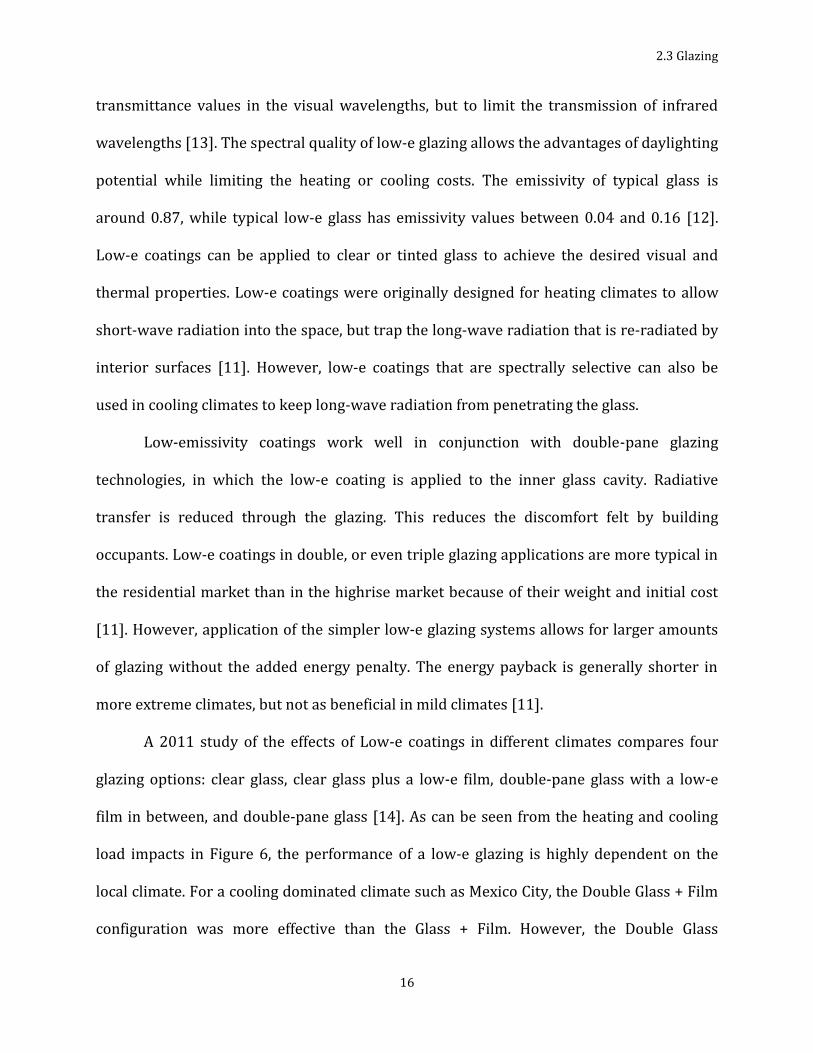
2.3 Glazing
16
transmittance values in the visual wavelengths, but to limit the transmission of infrared
wavelengths [13]. The spectral quality of low-e glazing allows the advantages of daylighting
potential while limiting the heating or cooling costs. The emissivity of typical glass is
around 0.87, while typical low-e glass has emissivity values between 0.04 and 0.16 [12].
Low-e coatings can be applied to clear or tinted glass to achieve the desired visual and
thermal properties. Low-e coatings were originally designed for heating climates to allow
short-wave radiation into the space, but trap the long-wave radiation that is re-radiated by
interior surfaces [11]. However, low-e coatings that are spectrally selective can also be
used in cooling climates to keep long-wave radiation from penetrating the glass.
Low-emissivity coatings work well in conjunction with double-pane glazing
technologies, in which the low-e coating is applied to the inner glass cavity. Radiative
transfer is reduced through the glazing. This reduces the discomfort felt by building
occupants. Low-e coatings in double, or even triple glazing applications are more typical in
the residential market than in the highrise market because of their weight and initial cost
[11]. However, application of the simpler low-e glazing systems allows for larger amounts
of glazing without the added energy penalty. The energy payback is generally shorter in
more extreme climates, but not as beneficial in mild climates [11].
A 2011 study of the effects of Low-e coatings in different climates compares four
glazing options: clear glass, clear glass plus a low-e film, double-pane glass with a low-e
film in between, and double-pane glass [14]. As can be seen from the heating and cooling
load impacts in Figure 6, the performance of a low-e glazing is highly dependent on the
local climate. For a cooling dominated climate such as Mexico City, the Double Glass + Film
configuration was more effective than the Glass + Film. However, the Double Glass

2.3 Glazing
17
configuration had the best overall performance. For Ottawa, the best overall performance
was the Glass + Film. The study also assessed the energy cost implications for the results
based on local heating and cooling costs. For Mexico City the double glass remained the
most successful design, but for Ottawa the double-glass + film configuration achieved the
lowest annual energy cost [14]. Because the cost of heating versus cooling costs for a given
location may differ, economic implications may not match the straight energy saving
characteristics of the glazing type.
This study shows a small sample of the potential energy savings available through
low-emissivity coatings. It only explores one specific metal compound, and two distinct
climates. The low-e market contains a wide variety of options of metal compounds and
glazing configurations. Clearly it is necessary to assess the implications for a given glazing
option for the specific climate. Low-e coatings can be extremely cost-effective in certain
circumstances.
A 1998 study by Sekhar, S.C. analyzes the energy performance and life cycle cost of a
range of types of reflective and low-emissivity coatings in double-pane glass [15]. The
study concludes that for a Singapore climate, the energy savings in terms of both HVAC
Figure 6: Cooling and heating energy loads for (a) Mexico CIty and (b) Ottowa [14]

2.3 Glazing
18
load and lighting energy are significant. The base case was a double pane float glass, and it
was compared to double glaze with heat reflecting glass and two kinds of low-e coatings.
The HVAC load savings can be seen in Table 1. The values are averages of the various tints
also included in the analysis. The study also claims that properly designed window systems
can potentially save 50-70% of the lighting energy, and 30-40% of the perimeter zone
energy with daylighting. Sekhar also showed the discounted payback period of the low-
emissivity glazings for this particular case to be 4 years, which is generally an acceptable
payback period for most companies. This again is one case, in a specific climate, with a
particular geometry, so savings would not be guaranteed for every case. However, this case
does show that savings through these surface coatings are possible.
Table 1: Energy consumption comparison [15]
Glazing Peak Cooling Load Total Load Savings From Baseline
Double Glaze Float Glass 496kW 1790 MWh
Double Glaze Heat Reflective Glass 405kW 1688 MWh 91kW, 102 MWh
Double Glaze HRG with Low-e 384kW 1643 MWh 112kW, 147 MWh
2.3.3 Insulating Glass
Insulating glass units can reduce heat losses compared to single glazing by at least
50% [12]. The concept behind insulating glass is that a gas pocket is created between
sheets of glass, limiting heat conduction, convection, and radiation through the window
surface. Radiative heat losses can be reduced from 0.85 to 0.1, or even lower through the
application of a low-e coating. A 12mm air cavity has a U-value of 3 W/m2K, while with the
addition of a low-e coating that same cavity can reach a U-value of 2 W/m2K [12].

2.3 Glazing
19
Gas-filled cavities have become standard practice for many residential applications,
and are used in limited commercial applications. The gases used to fill the cavity space
further reduce heat transfer through the glass. The most popular gas-fill is Argon gas
because of its relatively low cost [11]. Also used are krypton and xenon, though they are
less readily available and so have a much higher associated cost. The U-value of a 15mm
argon-filled double pane window with low-e coating is about 1.1 W/m2K, while a similar
krypton-filled pane yields a U-value around 0.8 W/m2K [12]. Triple pane windows offer
even further reduction in U-values. The lowest U-values can be achieved through evacuated
panes, in which a vacuum is created between panes. However, the structural stability of the
glass is difficult to achieve with evacuated panes, and the complexity of manufacturing is
cost-prohibitive. A vacuum glazing can cost up to 15% more than a standard double-glazing
with similar thermal properties [16]. However, evacuated glass can achieve heat transfer
rates two to five times less than gas-filled cavities [17]. With all the insulating glass types, it
is difficult to obtain a proper, long-lasting seal on the cavity. Manufacturing expenses are
high, which drastically limits the use of insulating glass on a large scale such as in a highrise
building.
A less common insulating glass category is referred to as transparent insulation
materials. The materials can be glass, polycarbonate, quartz foam, or any other type of
translucent material that allows for the creation of air spaces between the two external
panes of glass. A developing strategy is the use of aerogels, which has microscopic cavity
structures that allow for insulation values of R-12 to R-15, and allow visual transmittance
of around 90% [18]. Combined with low-e coatings, the aerogel panels could make
windows with U-values below 0.6W/m2K. However, development continues to overcome

2.3 Glazing
20
the barriers to a cost-effective manufacturing process, as well as the production of highly
transparent large panels [18]. There are many different configurations for the materials
within the cavity of transparent insulating material glazings. However, due to the complex
nature of these configurations, transparent insulation materials would likely not be used in
highrise buildings to a large extent.
2.3.4 Switchable Glazing
Another emerging technology is chromogenic glass, which responds to the
environment to produce advantageous glazing characteristics. The categories of
chromogenic materials are photochromics, thermochromics, electrochromics, and liquid
crystals [11].
Photochromic materials automatically reduce their transmission capacity in
response to an increase of incident UV light. The advantage to photochromic glazing is its
durability and capacity to reduce glare. A disadvantage is that it does not discern between
times when solar gains may be desirable, such as during the winter. The absorption
properties of photochromic materials also create uncomfortable heat gains and radiation.
At this time, photochromics are difficult to produce to scale, and are rare in large-scale
application, but research in this area is ongoing.
Thermochromic materials change state or properties when heat is applied. There
are several approaches to thermochromic glazing. Cloud Gel and TALD, two hydrogel
thermochromic products, have recently been developed. Hydrogels can have solar energy
transmission values of 0.8 to 0.9 in the low temperature state, while ranging from 0.05 and
0.4 when activated [12]. Care must be taken with hydrogels that freezing does not occur
when temperatures reach below freezing. Another approach to thermochromic glazing is to

2.3 Glazing
21
utilize plastics that begin gradually clouding between 25°C and 120°C [12]. Certain metal
oxides can also be used between the panes of glass, which can act as a low-e coating as
temperature increases [12]. The advantage of thermochromic glazing is that they reduce
overall and peak energy loads. They can also reduce glare and improve thermal comfort.
The disadvantages are that visible light is limited when the thermochromic glazing is
activated, and the life of these glazings is limited. The manufacturing process for
thermochromics needs much further development to make them economically feasible
[19].
Electrochromic glazing research has received the most attention in recent years.
Research to improve marketability and to assess the energy cost savings for electrochromic
windows is on-going [20-30]. Electrochromic glazing operates through the transfer of ions
to influence the visual and infrared transmission qualities of the material. Figure 7 shows a
cross-section of a product being developed by SAGE Electrochromics. Typical of most
electrochromic windows, the unit includes an electrochromic layer (EC), an ion conductor
layer (IC), and a counter electrode layer
(CE) sandwiched between two
transparent conductor layers (TC) [20].
When voltage is applied to the
transparent conductors, Lithium ions
travel through the conductor layer. The
electrochromic layer generally contains
a tungsten oxide, which reacts with the
lithium to form lithium tungstate, a light absorbing material [21]. The amount of change in
Figure 7: Cross-section of a SAGE Electrochromic window [20]
2.3 Glazing
22
the absorption is directly dependent on how much voltage is applied. The process is then
reversed when voltage is removed, and the window returns to the clear state. Low-
emissivity coatings can be used in conjunction with the other layers of the electrochromic
glazing to reduce the amount of the absorbed radiation that is emitted into the space. In
prototype testing at the Lawrence Berkeley National Laboratory, glazings reached a visible
transmittance (VT) range of 0.6-0.05, and solar heat gain coefficients (SHGC) of 0.42-0.09
[22].
Two of the largest advantages to electrochromic windows are that they offer a
greater extent of occupant control than other switching technologies, and they maintain
window views throughout the shading spectrum. The voltage application can either be
occupant controlled, or it can be controlled through a central building automation system,
connected to a variety of feedback devices. The initial cost for these systems is substantial,
not just for the glazing itself, but for the electrical and monitoring systems as well. Once
installed, the operating costs are relatively low. A recent study of electrochromic
prototypes by the Lawrence Berkeley Laboratory revealed that the prototypes would
switch with an applied voltage of ±3-5 V dc [22]. An ASHRAE study quoted that the
electricity needed to power and control 1500ft2 of electrochromic glazing per day is less
than what is needed to power a single 60W light bulb per day [21]. Electrochromic
technology also offers significant potential to reduce total and peak energy consumption.
The Lawrence Berkeley Laboratory testing predicts potential daylighting energy savings of
44% on average, compared to a case with blinds and no daylighting controls. The total daily
cooling loads with lighting heat gains included remained similar to the base case, but the

2.3 Glazing
23
peak loads were reduced by 19-26% with electrochromic windows [22]. The greatest
savings were the greatest for façades facing south, east, and west in hot U.S. climates [23].
There are many factors limiting large-scale application of electrochromic glazing.
The technology has shown to degrade in performance relatively quickly. Compared to the
long-term warranties on many other current glazing technologies, electrochromic glazing
does not measure up. The installation costs are still a concern, and companies such as SAGE
are continuing product development to make electrochromic glazing a viable option. A
1999 analysis by SAGE estimated that in order for significant market penetration,
electrochromic units must be sold at prices below $15/sq.ft, which they have yet to achieve
[24]. A cost-benefit study of a highrise residential tower in Hong Kong showed a 6.6%
savings on annual energy. However, it showed a benefit/cost ratio of 0.6, which means the
investment would not be economically beneficial [25]. The manufacturing process is still
quite complicated, which translates to increased cost. It is also still difficult to produce
large panel sizes that are dependable, let alone on a scale that would be required for
widespread application for highrise buildings. Switching time is a concern with
electrochromics; most current technologies require 5-10 minutes to switch from fully
colored to bleached states [26]. Current electrochromic technologies also display much
more difficulty in switching in low temperatures – on the order of 40-85 minutes [22]. In
variable climates, or on partly cloudy days, this switching time can cause problems for
system controls, and ultimately will negatively affect occupant comfort. While the colored
glass will mitigate some glare, current technology does not adequately intercept enough of
the glare, and secondary glare control may be necessary. There are many aspects of
electrochromic glazing that require improvement, but because of adaptability of control

2.3 Glazing
24
and potential energy savings, electrochromics are currently receiving the most attention as
a potentially feasible switchable glazing technology.
Liquid crystal panels operate similarly to electrochromic layers in that transmission
is changed via the application of an electrical charge. Liquid crystals without applied
voltage are scattered randomly throughout the cavity. When voltage is applied, the crystals
align themselves to permit the transmission of light [12]. There are two main approaches
to liquid crystal technology: suspended particle technology and micro-encapsulation.
Suspended particle technology is a thin cavity of liquid crystals between two sheets of glass
coated with a conduction material. Micro-encapsulation is the same concept, except the
liquid crystals are contained in tiny cavities [11]. The advantage to liquid crystal
technology is that the switching time is much faster than other switching glazings – 1 to 3
seconds [21]. A disadvantage to liquid crystals is that they are non-transparent when no
voltage is applied. This technology is also not stable in larger panels, against ultraviolet
radiation, or in extreme temperatures [12]. Currently liquid crystal technology is more
commonly used indoors and in automobile applications.
2.3.5 Directional Control
There are many options for external shading in order to control the direction of
incident solar radiation. However, a technique that is integrated into the glazing itself is a
holographic device. The holographic effect is achieved by 3-D laser etchings on a
photographic film, which is laminated between two glass panes [12]. The etchings can have
different configurations to achieve a variety of light dispersion and selection. For example,
equally spaced parallel lines will redirect the incident sunlight onto the ceiling, while
concentric elliptical lines will separate the light into individual spectral colors and

2.4 Shading
25
concentrates them on different focal points. The elliptical lines make it possible to regulate
the transmission of certain wavelengths (stopping infrared may be extremely useful) [12].
Holographic glass is often mounted to tracking louvers because the transmission of the
glass is dependent on the angle of incidence. Usually the louvers are programmed to track
the zenith angle of the sun [31]. Holographic glazing has been used on a limited scale in
only a few cases. The technology is extremely complicated to not only produce the glass,
but also to incorporate a low-maintenance, dependable louver system where necessary.
2.4 Shading
Shading devices are available in a wide range of forms – overhangs, side fins, light
shelves, blinds, louvers, and screens. Shading devices can be fixed or moveable, translucent
or opaque; they can be internal, external, or even between panes of glass.
The advantage to external shading is that it blocks or redirects the incident solar
radiation before it enters the building. Internal shades alleviate some glare problems, but
once the infrared radiation has passed through the glazing, the majority of it is dissipated
into the space, so they can cause problems with heat gain. External shading devices are
utilized less for highrise buildings because of the added construction costs, increased
maintenance, and aesthetic effects. Because there are generally large amounts of glazing on
contemporary highrise buildings, external shading devices could have a large energy
savings impact, but they could also drastically alter the view characteristics of the façade.
External shade design is a complex process and is heavily influenced by shade design,
façade orientation, and glazing type [32]. Architects often prefer to maintain continuity in
façade design, but they are now exploring new and creative ways to address the different

2.4 Shading
26
energy needs of each façade orientation. Some architects have even designed the entire
building footprint such that portions of the building provide self-shading [33].
Internal shading devices are common because they are an inexpensive solution for
glare control and they are generally manually operable, which increases occupant control.
Occupant control can have its drawbacks as well, as blinds or shades may remain drawn
when they are not needed, reducing potential daylighting or heating benefits. There are
systems available for automated blinds, which reduce the amount of user control, but are
much more easily optimized for energy saving practices.
Tzempelikos, A. performed a study in 2007 to determine the energy saving potential
of an external roller shade device and lighting control for a south-facing façade in Montreal,
Quebec, Canada [34]. The study optimized the window-to-wall ratios for the south façade at
30%. The transmittance of the shade was also optimized as 20%. Results would vary for
other façade orientations and window-to-wall ratios. The study analyzed the energy effects
of active versus passive lighting controls for the building, and compared passive control
versus active control of shades. Passive control was modeled as the worst-case scenario of
shades closed during 100% of working hours. Active automatic controls optimized the
Figure 8: Comparison of energy consumption for shading and lighting control [34]

2.5 Double-Skin Façades
27
daylight potential, and remained open unless the incident solar radiation posed a glare risk.
Figure 8 shows the potential savings from automatic shading and lighting control. The use
of shading control in particular results in a 50% reduction of the cooling load compared to
no shading control, and a 12% reduction in total annual energy consumption.
Actual savings would depend on what kind of HVAC systems were utilized in
conjunction with the shading device. Alternative glazings were not assessed in this case,
which would impact the results. Shading devices are sensitive to orientation, surface area
ratio, and climate, so results could be more or less pronounced based on change in any of
these variables. A 1998 study by Lee, E. at the Lawrence Berkeley National Laboratory
performed a similar analysis for a building in California [35]. This study drew similar
conclusions regarding a dynamic automated venetian blind system. They were able to
produce 1-22% lighting energy savings, 13-28% cooling load reductions, and 13-28% peak
cooling load reductions annually compared to a static blind with the same daylight controls
[35]. These studies clearly show that shading devices and their controls combined with
lighting controls can potentially have a large impact on the energy consumption of a
building.
2.5 Double-Skin Façades
There has been a dramatic increase in research pertaining to double-skin façades in
the last decade. A double skin façade (DSF) can take a variety of forms, but the most basic
DSFs are made up of two adjacent glazing units with solar control devices in between [36].
The double-skin façade is basically an exaggerated version of double pane glass combined
with the building’s ventilation and shading systems. The original goal of DSFs was to

2.5 Double-Skin Façades
28
provide an effective sound barrier, and
the technology has been developed to
include daylighting and HVAC benefits.
The recent growth in attention for DSFs is
because of the potential natural
ventilation capabilities, and occupant
comfort advantages associated with this
type of façade. However, most European
architects and engineers continue to
advise clients that the main benefit is not
necessarily energy efficiency, depending
on the circumstances [37]. The physics
associated with the DSF makes modeling and prediction of this technology extremely
difficult (Figure 9). Another difficulty is that DSFs vary widely from one design to the next.
DSFs can span multiple floors, or be contained to one floor. The cavities can range from 15-
150cm deep, and a variety of glazings and solar shading devices can make up the DSF
system [38]. Façades can be naturally ventilated, if design properly and climate The success
of DSFs depend on careful control of the integrity of the envelope, which translates to less
occupant control and a more extensive sensor and controls system.
Although double-skin façades have already been implemented in several locations,
the benefits and performance characteristics of ventilating façades are still widely debated.
Double-skin façades have been implemented more often in Europe because of higher
expectations on behalf of occupants in terms of view and daylight [36]. DSFs potentially
Figure 9: Thermodynamics of a DSF [34]

2.5 Double-Skin Façades
29
allow for greater perimeter-to-floor ratios with less negative impacts on occupant comfort.
DSFs have been used most often in new building construction, but there are increasing
cases of retrofit applications [39,40]. Existing double-skin façades have been the focus of
performance measurement and modeling
verification in order to better understand exactly
how the heat transfer occurs. A study by Corgnati,
S. for the application of double-skin façades in
Torino, Italy monitored an existing DSF for two
years. The conclusion was that while the DSF
displayed energy performance on par with other
glazed façades, but was not competitive with
traditional windowed opaque façades [41].
Hamza, N. performed a simulation analysis of DSFs in hot, arid climate. The study showed
that a reflective DSF had lower cooling loads than a reflective single-skin façade [42]. Altan,
H. et al. performed a similar analysis in Sheffield, England, and recommends DSF designs on
the basis of their use of passive solar energy and positive work environment [43]. In 2009,
ASHRAE released a study of the Pearl River Tower in Guangzhou, China. The article
outlines the impacts of certain design decisions for DSFs. The case study shows that the
room conditioning load and cavity ventilation load is lower than the cooling load for a
single façade. However, if the cavity air were returned to the HVAC system and
recirculated, the load would be higher than that of the single façade [36]. Cetiner, I.
compares the energy performance and economic tradeoffs between efficient single-skin
façades and efficient double-skin façades in moderate climates, such as Istanbul. The study
Figure 10: Cross-section of one DSF strategy [5]

2.6 Thermal Concerns
30
concludes that the most efficient DSF design is 22.84% more efficient than the most energy
efficient single-skin configuration. However, it also showed that the most cost effective
single-skin configuration is 24.68% more cost effective over its lifetime than the most cost
effective double-skin configuration [44].
The Cetiner study brings up an important drawback to the ventilating façades,
which is the significant initial investment required to produce a highly energy efficient
double-skin façade envelope. Other disadvantages to double-skin façades are potential
excessive thermal gains and visual discomfort as a result of poor design [36]. Because of
the wide variety of design options and the complicated nature of predictive modeling, it is
difficult to produce a reliable, energy efficient DSF design. Another drawback is that dust,
noise, condensation, odors, and even smoke from potential fires can be problems within
the DSF cavity. If the cavity is naturally ventilated, there is increased risk of these potential
problems, which leads to the increase in maintenance costs [36].
There are many potential advantages to the double-skin façade, as well as many
potential drawbacks. The most important lesson learned from the various studies of DSF
performance is that the façades must be tailored for each individual project and climate in
order to reach maximum efficiency.
2.6 Thermal Concerns
2.6.1 Thermal Bridging
In highly glazed façades much of the focus is concentrated on the glazing portion in
order to reduce the negative thermal impacts. However, even in façades with the highest

2.6 Thermal Concerns
31
window-to-wall ratio, there exists the potential for thermal bridging through the opaque
section of the façade. Window frames and curtain wall fastenings can be sources of heat
loss through thermal bridging. Research is ongoing to determine the extent of the impacts
of various glazing fastening strategies on thermal loss [45-47]. Song, S.Y. et al. performed a
study in 2007 on the performance of several insulation strategies for aluminum curtain
wall fasteners in highrise buildings in Korea [45]. Compared to the existing fastener
strategy, they found 8.14% reduction in heat loss by coating the upper part of the fastener
with urethane foam and the lower part with insulation paint. A Gustavsen, A. study on
various high performance frame systems examined two current curtain wall systems that
yielded overall U-values of 0.73 and 0.65 W/m2K [46]. These U-values are still two to three
times better than typical U-values of insulating glass, but slightly higher than U-values that
can be achieved through opaque, insulated façades (0.2-0.3 W/m2K) [46]. While thermal
bridging effects should be considered with highly glazed façades, the thermal bridging of
the glazing section are much more significant than through the other façade materials.
2.6.2 Occupant Comfort
A major thermal concern with curtain walls is the implications of large amounts of
glazing on occupant comfort. As previously discussed, the increased view and daylighting
from highly glazed façades are generally positive in terms of occupant satisfaction.
However, the heat gains, glare potential, and draft concerns associated with curtain wall
design generally negatively impact occupant satisfaction. Occupant comfort is one of the
most difficult standards to quantify, and it is equally difficult to attempt to predict.
Occupants will subconsciously be affected by dozens of external factors at once, and
preferences for what is “comfortable” can vary significantly from one person to the next.

2.6 Thermal Concerns
32
The most common quantification for thermal comfort is PMV (percent mean vote) and PPD
(predicted percentage of dissatisfaction) [10]. Glass surface temperature and incident solar
radiation are two of the most common sources of problems of occupant comfort in glazed
façades. Several recent studies have examined the occupant comfort associated with
glazing, as well as strategies for improving occupant satisfaction.
Singh, M.G. et al. examined 15 different glazing types in order to quantify the
impacts of different tinted, insulated, and reflective glazings on occupant comfort [10]. This
study mostly examined the thermal effects of incident solar radiation and resulting
temperature changes in the space. They tested the glazings in a variety of Indian climates
throughout the year. Five different
tinted single pane windows were
tested, as well as 10 double-pane
windows with a variety of
configurations (tinted, absorbing, low-
e) and U-values. PPD was calculated
based on the ISO standard equation
7730, with variables such as mean
radiant temperature, air temperature,
transmittance, incident radiation,
convection coefficients, metabolic
rates, and human mechanical
efficiency. Figure 11 and Figure 12
Figure 11: PPD for cold and cloudy climate of Shillong [10]
Figure 12: PPD for hot and dry climate of Jodhpur [10]

2.6 Thermal Concerns
33
show the results of two types of climates for the range of glazing types. As is evident, the
effectiveness of the glazing is dependent on climate, further enforcing the necessity of
climate-specific design choices. For the hot and dry climate, the double pane windows with
absorbing film produced the best results, while the single glazing showed up to 80%
dissatisfaction. For the cloudy, cold climate, the single panel glazing and low-emissivity
double-panel glazings produced the most satisfaction, while the absorptive double glazing
produced the most dissatisfaction. The solar PPD for the cold climate was shown as
negative because the warming effect from the incident solar radiation is actually a positive
attribute. As can be seen from the variety of results of this study, the choice in glazing can
dramatically impact the satisfaction of the occupants.
In a 2011 study, Hwang, R.C. and Shu, S.Y. assessed the impact of building envelope
regulation on thermal comfort and the energy-saving potential of PMV-based comfort
control in glass-façade buildings [48]. The analysis was performed for the climate region of
Taiwan. Simulations were performed with a variety of glazing types, overhangs, and glazing
areas. For glazing type, it was shown that discomfort increases with higher transmittance
because of incident solar radiation to the space. Discomfort also increases as a result of
absorption because of the increased surface temperature of the glass. The total radiation
varied with the SHGC in a quadratic relationship. It was also shown that discomfort
increases with increased window size due to the radiant heat of the surface and the
increased solar radiation – the solar radiation accounting for a larger fraction of the total
radiation as the window area increases. They concluded that it is possible to achieve
energy conservation and satisfactory levels of thermal comfort through careful façade

2.6 Thermal Concerns
34
design. It was also concluded that the energy savings through PMV-based control in areas
with high cooling loads were limited, but increased in potential as cooling load decreased.
The other common source of occupant discomfort with highly glazed façades is the
induced draft from surface temperature of the glass. The occupant discomfort caused by
radiation from surface temperature in cooling conditions was discussed previously.
However, in heating climates it is often necessary to utilize radiators and convectors below
or near the windows to mitigate the effects of cold drafts from the cold glass surface
temperatures. Ge, H. et al. studied the effects of the cold drafts created by two types of
glazing on occupant comfort [49]. Heiselberg, P. has also performed research in this area
[50, 51]. The cold draught is caused because of a temperature differential between the cold
glass surface and the warmer room air. A conventional double glazing unit was compared
to a high-performance glazing unit. The results showed that occupants closer than 2m from
the wall experienced discomfort from drafts [49]. Heiselberg suggests that structural
components be used to work as obstacles to break down the convective boundary layer
and reduce the draft. Ge suggests the use of an overhead diffuser to break up the boundary
layer. The HVAC load impacts of this approach have yet to be determined. He also suggests
the use of a better-insulated glass panel. Besides the conduction benefits of a well-insulated
window, a study by Larsson, validates the conclusion that improved insulation will increase
the surface temperature of the glass, reducing the convective losses [52]. He also suggests
that improved thermal performance of the window reduces, or even eliminates the
necessity for HVAC systems below the windows. Reduction of the HVAC system not only
potentially reduces the load, but also increases the amount of useable floor space.

2.7 Ventilation and HVAC
35
The influence of shading devices on thermal comfort was discussed previously (2.4
Shading). Solar shading devices act to mitigate glare concerns, but also prevent incident
solar radiation from being absorbed by the glazing and/or being transmitted into the room
causing uncomfortable solar gains [9,34,53]. Shading devices must be optimized for a given
climate, much like most façade characteristics. Other simple strategies such as assigning
occupied zones away from the glazed surface can act to improve overall occupant comfort,
but this strategy often limits the flexibility of the floor plan, and is simply not possible in
other situations.
Optimization of the various façade improvement interventions will result in a more
energy efficient building and increased occupant comfort. The bottom line for most
building owners is not only to obtain tenants, but also to retain them. Occupant comfort is a
large part of that equation.
2.7 Ventilation and HVAC
2.7.1 HVAC loads and Energy Consumption
The quantification of the advantages of these advanced façade technologies is
almost always in terms of heating and cooling load impacts. There is concern on behalf of
the owners for initial cost, but generally in buildings the operating costs vastly outweigh
the initial costs over the building’s lifetime. According to a technical journal from the
Council on Tall Buildings and Urban Habitat, for a building with a 50-year lifespan, the
initial costs account for 12%, maintenance counts for 4%, and operation costs account for
85% of the lifetime costs of the building [54]. The exact amount of the HVAC costs depend

2.7 Ventilation and HVAC
36
on climate and building design, but it does account for a vast majority of the energy
consumption by the building [33].
Annual energy savings are crucial for reducing operational costs, but reduction in
the peak load conditions can provide dramatic cost savings as well. The HVAC system must
be sized for the most extreme heating and cooling requirements. A reduction in the peak
energy requirements for the same building will result in initial and annual cost savings on a
smaller central heating and cooling plant, as well as smaller ducts, pipes, and other system
equipment. For this reason, proper building energy modeling and equipment sizing is
crucial to the energy efficiency of the building. There continues to be new research and
development in energy efficient HVAC system equipment.
A variety of systems have been used throughout recent history for heating and
cooling of highrise buildings. Variable-Air-Volume (VAV) systems are one of the most
common systems in highrise buildings. Some buildings will utilize low-temperature VAV
systems, in which the supply air is much colder than usual (32-48 degrees Fahrenheit) to
allow for lower supply air volumes. Duct sizes can be reduced, however, special measure
must be taken to insulate vents and prevent condensation. Because there are many times in
highrise buildings where the exterior zones require heating while the interior zones
require cooling, many times the VAV systems are supplemented by hot-water or electric
baseboards, or by a reheat system [55]. Another VAV strategy is to implement VAV units in
the interior zones and supply the heating and cooling needs of the exterior zones with fan-
coil units. This allows for reduction of the mechanical systems supporting the VAV system,
but does require additional mechanical pumps and heat exchangers for the fan coil units.

2.7 Ventilation and HVAC
37
However, it is another solution for the issue of highrise buildings requiring heating and
cooling simultaneously.
Displacement ventilation has grown in popularity as well, from its energy-saving
potential. Usually the air is introduced into the space at the floor level, thereby encouraging
stratification. The concept behind displacement ventilation is similar to that of the UFAD
systems. The system is configured to condition the occupied space. In most buildings, air is
delivered from above. This generally conditions the air from floor to ceiling throughout the
building. Because of stratification with the displacement ventilation, the space is only
conditioned to about 1.8m above the floor height, which is much a little over half the typical
floor-to-ceiling height [37]. The overall volume of conditioned space is reduced,
theoretically limiting the HVAC requirements to each space. This system also removes
contaminants to the upper region of the room, away from occupants rather than diffused
throughout the space. A popular method of displacement ventilation, called under-floor air
distribution (UFAD), is under much scrutiny for proof of the benefits assumed to
accompany the system. There are benefits to stratification of the room air with UFAD
systems, but also potential health and thermal conduction concerns due to the
concentration of hot air and contaminants at the ceiling. It is difficult for UFAD systems to
control the conditioning of perimeter zones separately from interior zones. There are also
maintenance concerns with the cleanliness and limited access to the under floor systems.
UFAD systems are climate dependent, and it are still a relatively new technology, so they
are not currently widely implemented. They can be more cost intensive to install, but they
also require less ductwork, which can limit the expense of the system [55].

2.7 Ventilation and HVAC
38
Some tall buildings with glazed façades utilize a central atrium with the stack effect
to provide some natural ventilation for the space (See Natural Ventilation). Stack effect
occurs when outdoor temperatures are lower than the inside temperatures. Cool air flows
in the lower floors and rises through the building as it is warmed. In highrise buildings this
effect can be more pronounced because of the height of the buildings. Stack effect can be
utilized to ventilate, but in highrise buildings it can also cause pressure issues and can
make it difficult to keep the building uniformly heated or cooled [55]. Mixed-mode
operational systems switch to a mechanically ventilated system during the winter to
mitigate heat losses [37]. A mixed-mode trombe wall system could be utilized to provide
insulation and heat through a double-skin façade arrangement.
These and other energy-saving HVAC systems have been gaining in popularity in
recent years, but further research is necessary to gain a more accurate cost-benefit analysis
for implementation in highrise buildings.
2.7.2 Natural Ventilation
The first generation of highrise buildings had much more thermally massive façades,
which were naturally ventilated generally through operable windows. As façade design
changed, mechanical ventilation became more and more heavily relied on. Because of the
fuel consumption and high energy cost associated with mechanical systems, there has been
an increasing amount of attention for passive approaches to building HVAC. Natural
ventilation has been revived as a potential energy-saving HVAC intervention.
Natural ventilation in highrise buildings harnesses the potential of buoyancy and
the stack effect to remove heat from the building envelope [56]. The configuration of each
natural ventilation system is unique to the building layout, orientation, thermal mass, and

2.7 Ventilation and HVAC
39
façade design. Climate also plays a large role in the design and success of natural
ventilation systems. Because natural ventilation is tied intrinsically to the building design,
it is most often carried out in new construction. Yeang, K. provides guidelines for
implementation of natural ventilation systems in his book, The Green Skyscraper: The Basis
for Designing Sustainable Intensive Buildings [40]. He suggests that the building orientation,
surface to volume ratio, and footprint must all be tailored for maximum natural ventilation
from the beginning of the design process to ensure the greatest success.
Natural ventilation can be integrated into the daytime HVAC strategy, or it can be
used separately in a “night-flush” strategy. Daytime natural ventilation under the right
climate conditions improves the occupant comfort and satisfies the code ventilation
requirements for fresh air. Nighttime ventilation takes advantage of the cooler night
temperatures to remove heat loads that have been absorbed by the thermal mass in the
space. With this strategy, the thermal mass is then “activated” at night and cooling is
released throughout the day. Nighttime ventilation under the right circumstances will
reduce the peak and total cooling load, and in certain climates and building designs it can
eliminate the need for mechanical air-conditioning [56].
There are several potential configurations for natural ventilation, and the basic
concepts can be adapted to individual designs. Natural ventilation can be used in different
configurations in isolated floors with cross flow ventilation or in individual rooms with
single-sided ventilation (Figure 13). The disadvantage to the isolated approach is that it is
usually only effective when the width-to-height ratio is less than 5 for each space [57]. This
could limit the complete reliance on natural ventilation for spaces that do not comply.
However, individual spaces are typically simpler to model and predict performance. The

2.7 Ventilation and HVAC
40
double-skin façade works well with the concept of natural ventilation because the second
façade provides protection from some of the noise, wind, pollutant and thermal concerns
associated with single skin façades and natural ventilation. It allows for a more controlled
form of natural ventilation. Double-skin façade systems can be isolated to single stories, or
they can span multiple stories. Both approaches are adaptable for natural ventilation. The
GSW Headquarters in Berlin is an example of the double-skin façade and natural
ventilation. This design uses a west-facing DSF as a thermal flue. As the air is heated and
rises due to buoyancy, it draws fresh air from the cooler, east façade. The GSW building is
naturally ventilated for around 70% of the year [5]. The Commerzbank building in
Frankfurt takes a different approach by utilizing an atrium for the thermal flue (Figure 14).
The Commerzbank building relies on natural ventilation more than 80% of the year. The
disadvantage to this approach is that high pressure differences can be created by the
buoyancy effect [25]. To mitigate this effect, the spaces can be divided into separate
segments that are individually tied to the outdoors.
Full natural ventilation represents the greatest potential for HVAC operation and
equipment savings. However, even the most careful designs may not be able to rely on
Figure 14: Natural ventilation through an atrium [55] Figure 13: Natural ventilation in isolated spaces [55]

2.8 Integrated Design Process
41
natural ventilation year round. Mixed-mode ventilation allows for some of the energy
saving advantages of natural ventilation, but addresses both heating and cooling loads.
Most buildings using natural ventilation would need to utilize a supplemental HVAC system
to meet year-round loads. It is hoped that a successful natural ventilation design will allow
the HVAC system to be downsized as a result of lower peak loads. Yeang, K. compares
energy consumption of a typical air-conditioned office to good practice, open-plan natural
ventilation. With a base-case load of 390 kWh/m2, he expects that natural ventilation could
produce the same results with only 136 kWh/m2, or 65% energy savings per unit area [37].
Similar to the other building components, design of a natural ventilation system requires
careful planning and optimization for the particular climate and building use in conjunction
with the other building components in order to produce a successful design.
2.8 Integrated Design Process
A common theme with façade design is that everything is climate dependent, and
design choices for one component often affects the design of another, seemingly unrelated
component. In an effort to produce the most energy efficient building design, integrated
design is essential. Façade design is integral to the tangled web of systems within the
building design (Figure 15). The performance of the façade and supporting systems are
closely tied to the building orientation, floor layout, and location. These are variables that
are generally decided very early on in the design process. In order to have the greatest
opportunity for energy savings, façade design must be considered in conjunction with the
other variables at the beginning design stages. For example, a footprint that is optimized
for solar potential will influence the choice of glazing; the glazing that is optimized for both

2.8 Integrated Design Process
42
its thermal characteristics will reduce the size and nature of the HVAC needs; the glazing
that is further optimized for daylight potential will reduce the electrical lighting load, which
will decrease the sensible heat gains, which will further reduce the size of the HVAC
system. If the footprint was not addressed early on, the energy consumption savings from
the glazing could potentially be drastically reduced, which would in turn affect all the other
potential benefits.
Tzempelikos, A. et al. performed a simulation and optimization of façade design,
lighting design and control, and HVAC components for a Montreal institutional building
[59]. Because they performed this service in the beginning design phase, they were able to
influence factors such as window-to-wall ratio, shading components, and daylight potential
rather than simply being able to select the most energy efficient glazing. Because of the
Figure 15: Tall Building System Integration Web [58]

2.8 Integrated Design Process
43
compounding nature of effective façade, daylighting, and HVAC design, they were able to
reduce the baseline peak cooling load by up to 36%, and eliminate the need for perimeter
heating altogether [59].
Effective integrated design first requires a paradigm shift. Most architects and
engineers have already acknowledged the benefits of integrated design. It is not always
possible because of client constraints, but integrated design from the start makes it easier
for the engineer to produce the best results possible. The other major component involved
in system design in the conceptual stage is the necessity of simulation and modeling
capabilities. Case studies can provide a baseline for many initial design decisions. If there
were a more extensive, centralized organization of case studies and simulation research,
then case studies could probably be used more extensively farther into the design process.
However, because performance characteristics are unique to each design situation, case
studies do not produce the hard numbers often required to convince the building owner to
pursue an initially costly, yet energy efficient design.
There have been many recent published journals and research papers that assess
different façade technologies in a variety of climates, and most of them utilize at least one
type of simulation software. There is a large amount of new research coming out of Hong
Kong and China because the recent surge in highrise construction in Asia, and the need for
energy efficient new construction and retrofits [25, 60-70]. Bojik, M. and Yik, F. from the
Hong Kong Polytechnic University have done extensive research and simulation of glazing
technologies in the hot, humid climates of Hong Kong and other areas [25, 60, 65, 67]. Lam,
J. and Wan, K. have also contributed to the research through the City University of Hong
Kong in the simulation and design recommendations for building envelopes in a variety of

2.8 Integrated Design Process
44
Asian climates [61, 62, 65]. Tzempelikos, A. has contributed numerous publications about
the relationship between glazing and thermal systems through simulation [34, 53, 59, 71].
Lee, E. out of the Lawrence Berkeley National Laboratory has published many simulation-
based reviews of various types of high performance building façades [23, 35, 56, 37, 72].
The Lawrence Berkeley National Laboratory and its associates have published numerous
building case studies, technology reviews, market assessments, and a variety of simulation-
based research. A variety of façade technologies have been assessed in a variety of climates:
the hot and humid of Hong Kong, the temperate climate of California, and the heating
dominated climate of Russia [73]. These studies can be utilized as case studies to guide
design decisions for similar climates, but design decisions will change based on building
orientation, façade materials, and specific building purposes. Building energy simulation is
one of the most common ways engineers, architects, and researchers quantify results and
justify conclusions.
One of the largest barriers to effective energy-efficient design is that simulation is
often time consuming and complicated. Some of the most widely used simulation software
for façade simulations is EnergyPlus, BLAST, DOE-2, and HTB2. EnergyPlus is more
prominent in the recent simulation-based research. These programs, while powerful, are
still quite complicated. This adds time and, consequently, cost to the already complex and
extensive design process. Efforts have been made to more seamlessly integrate building
energy simulation into the design process, and improve optimization. A 2004 study
assessed the advantages of an integrative building simulation program – one that modeled
lighting, energy, ventilation, and fire and smoke risks [74]. The extensive modeling would
be time consuming, but it would provide comprehensive building monitoring, and

2.9 Code Compliance
45
improved optimization of systems. Zheng, G. et al. suggest a “grey relational method,” which
is a vector analysis method to aid the decision-making process for incomplete or uncertain
systems [69]. It is also helpful in situations where alternatives are difficult to quantitatively
compare. The study concludes that the improved grey relational projection theory for
façade design, but it is currently not commonly used. Tzempelikos, A. presents a
methodology for a systematic approach to the selection of glazed facades in conjunction
with consideration for the heating and cooling implications [71]. It is intended to be an
integrated approach, ideally implemented at the beginning design phase. Design and
consulting companies are constantly searching for new ways to improve their processes.
However, the research previously referenced shows the invaluable nature of energy
simulation in guiding the choice of façade alternatives.
2.9 Code Compliance
Three international organizations have developed the most commonly accepted
building codes [75]. The most commonly used code in the United States is the ASHRAE/IES
90.1 is a code for the energy efficient design of new buildings, except for low-rise
residential buildings. The code stipulates the heating, ventilation and air conditioning
requirements, occupant comfort standards, and energy consumption standards. Standard
90.1 stipulates a maximum window-to-wall ratio for commercial buildings based on the
climate, internal loads, and window transmittance. The International Energy Conservation
Code is another set of commonly used standards focusing on energy efficiency. The IECC
specifies window-to-wall ratio based on climate, R-value, and heating degree-days. It also
specifies the SHGC for window systems including framing for different kinds of glazings.

2.9 Code Compliance
46
The third set of codes is from the Chartered Institute of Building Services Engineers, or
CIBSE. The window-to-wall ratios are determined based on building type. It also sets
standards building energy efficiency, lighting, HVAC, fires safety, and sustainability.
The infiltration of a building can have a large impact on the safety and energy
consumption of a building. For this reason, building codes have established standards for
air tightness for buildings. ASHRAE 90.1-2007, which is cited by many current building
codes in the United States requires air leakage for fenestration to be less than 0.4 cfm/ft2.
The IECC 2006 Code specifies requirements for curtain walls in particular. The IECC
requires air leakage of less than 0.3 cfm/ft2 of glazing area. Both documents comment on
the necessity of sealing all joints with caulking or other sealants. These standards are
helpful for energy efficient design of buildings, but a recent ASHRAE Journal article by Colin
Genge comments on the difficulty of actually testing and proving these air tightness values
in a highrise building [55]. Typically the standards of the IECC and ASHRAE are based on a
standard ASTM (American Society for Testing and Materials) test procedure requiring
certain test pressure. For highrise buildings it is difficult to maintain a uniform building
pressure throughout the entire building because of stack effects and wind effects that
change as heigh increases. In the article, Genge suggests that the testing procedure must be
tailored to the needs of a highrise building. This shows that, while there may be air
tightness standards in place, highrise buildings likely need more attention in the form of
specific tightness requirements and testing procedures.
With regards to other building design criteria specifically relative to highrise
buildings, ASHRAE has published a chapter called “Tall Buildings” in the ASHRAE Handbook
– HVAC Applications. This document outlines a variety of design concerns that are specific

2.9 Code Compliance
47
to highrise buildings such as stack effect and fire protection. It has rules of thumb for
design practices and general guidelines.
The International Building Code has included a portion specifically relating to the
regulations placed on “tall buildings.” These codes focus mostly on fire and safety
requirements of highrise building designs. Much of the code is dedicated to fire resistance
measures, evacuation strategies, and fire containment. September 11, 2001 caused these
and similar codes to be re-evaluated because of the catastrophic collapse of the World
Trade Center. Safety for highrise buildings is a complicated issue, and one that is highly
regulated by codes. There are not as many code requirements for HVAC systems and façade
types specifically for highrise buildings.
Governments around the world are beginning realize the importance of energy
efficiency in the building realm. Because many governments already have a system of
requirements in place for building codes, it provides a platform for introducing new
programs to encourage energy efficient options. The European Commission has begun to
require building energy labels and regular inspection of air conditioning plants to
encourage energy efficiency and proper equipment maintenance [76]. The UK has
implemented these strategies as part of a plan to reduce the annual carbon footprint. The
United States Green Building Council has implemented the Leadership in Energy and
Environmental Design (LEED) certification program, which has become a popular incentive
program for implementing energy efficient building technologies. The LEED system is a
rating system that allows buildings to receive certification on a scale of energy efficiency.
The LEED system is not a code standard, but it does help direct the design process toward
more energy efficient measures. It has become almost a status symbol for buildings,

2.10 Case Studies
48
increasing its appeal to tenants or clients. It has been shown that energy efficient buildings
are occupied faster, and can be cost effective if designed properly. It is the intent of the
LEED certification system to incentivize design choices towards energy efficiency.
2.10 Case Studies
2.10.1 Energy Efficient Highrise Retrofit: The Empire State Building
The Empire State Building is one of the most recognizable skyscrapers in the United
States, and possibly the world. It was recently the subject of a large retrofit design process
to improve the energy efficiency of the façade. The building owner was committed to a
profitable design, but he was also committed to energy efficiency from the beginning of the
retrofit process [77]. The Empire State Building opened in 1931, at 1472 feet tall. It
maintained the record for the world’s tallest building for over forty years [5]. This office
building retrofit was not just intended to improve the energy efficiency of the Empire State
Building. The owner was committed to making the retrofit a model for future retrofits of
similar, inefficient buildings [77]. Rocky Mountain Institute, Jones Lang LaSalle, Johnson
Controls, and the Clinton Climate Initiative were the major organizations that were
involved or consulted in the retrofit.
The Empire State Building (ESB) retrofit design team took an integrated approach
throughout the process, in what they called a “deep” retrofit [78]. The first step was to
assess the existing systems and energy usage of the building using eQUEST. They then
generated over 70 potential interventions that could meet the goal of 68% of the existing
energy usage. 17 implementable strategies were identified, which were modeled and used

2.10 Case Studies
49
for an analysis of net present value for each intervention. The process was extremely
collaborative from the building owners, to the research organizations, to the building
maintenance staff. Careful planning and strategic assessment of alternatives led to a final
design recommendation that was both energy efficient and cost effective.
The planning team attempted to balance the reduction in energy use with financial
returns. Eight measures were eventually selected [78]. First the façade was updated. The
ESB façade was made up of insulated glass. All 6,500 windows were planned to be removed
and updated with a suspended coated film and gas filled. Radiative barriers were installed
behind existing perimeter radiator units. The existing window-to-wall ratio is very difficult
to alter, especially in more massive exteriors like the ESB. The extent to which daylighting
can be effected in retrofits is generally limited. However, control systems for the lighting
systems were designed to take maximum advantage of available daylighting, complete with
occupancy sensors and task lighting. A new energy efficient demand control ventilation
system with VAV units was designed. The existing control system was upgraded to digital
and would offer greater control of the new and existing systems. Also a new tenant energy
management strategy was planned, which would provide more in depth feedback for
tenant energy use, hopefully reinforcing the daily practice of energy efficiency. One of the
most significant sources of savings was in the installation of a smaller chiller plant. Because
of the integrated design approach, the cooling load was reduced by 1,600 tons, leaving the
existing chiller vastly oversized. The ESB owners had been planning to replace the entire
system, but they were now able to simply update the system, saving up to $17 million
initial equipment costs. The final design plan would cost $13 million initially, and provide a
38% reduction in energy use, and annual energy savings of $4.4 million.

2.10 Case Studies
50
Clearly the retrofit efforts in the Empire State Building yielded not only
environmental benefits, but also will provide financial benefits for the building owners for
years to come. One of the goals of the ESB project was to form a process and provide the
tools necessary for other highrise buildings to follow suit. Since the Empire State Building,
interest in highrise retrofits has increased greatly. In 4 years, another U.S. highrise icon will
be receiving an extreme renovation of its own. The Willis Tower (formerly the Sears
Tower) will be undergoing massive renovations to produce the annual energy savings up to
80% from the baseline [79]. The 16,000 windows on the building’s exterior will receive
updates to increase the insulation value, saving up to 60% of heating energy. Daylighting
capacity will be expanded to allow for savings of up to 40% of the existing lighting energy.
Successful, high-profile energy retrofits in highrise buildings will only serve to reinforce
the fact that energy efficient measures are affordable and effective for buildings at all
stages.
2.10.2 Energy Efficient New Construction
The Commerzbank, built in 1997 in Frankfurt, Germany is one of the first of many in
the new generation of ecological highrise designs [4]. The goal in the design of the
Commerzbank tower was to build the first high-rise in the world that utilized natural
ventilation and at the same time natural lighting. Integrated design was used to ensure that
the façade, floor plans, and HVAC strategies work en tandem to produce an energy efficient
final product. The tower consists of a triangular ground plan with a segmented atrium that
runs the length of the building. The energy-efficient façade reduces the heat gains, making
utilization of the natural ventilation more effective. The tower is able to utilize natural
ventilation for up to 80% of the year [4].

2.11 Application
51
The Hearst Tower, commissioned in 2006, was the first LEED Gold certified
skyscraper in New York City. In order to achieve a design that is 26% more energy efficient
than the typical construction methods, the 600-ft tower utilizes a wide range of ecological
building design measures [80]. The lightweight, diagonal external structural braces allow
for large, unobstructed view glass and an open floor plan. These measures allow for
maximum light penetrability into the space. The façade is enclosed by low-emissivity glass
that reduces the amount of solar gain into the space. The energy efficient façade combined
with a lighting control strategy helps to further reduce the energy consumption of the
Hearst Tower.
The Comcast Center in Philadelphia was the tallest LEED certified building in the
United States at the time of its 2009 commissioning [81]. This is achieved through a variety
of energy efficiency measures, including an energy efficient façade design. The glazing for
this building is a high-performance, ultra-clear, low-iron glass [82]. The glazing blocks 60%
of solar heat gains, while allowing in 70% of the visible light. This allows for a drastic
reduction in heating and cooling equipment and operational costs. The building also
incorporates sunscreens and louvers to optimize daylight. Lighting and occupant sensors
combined with an energy efficient control strategy take full advantage of the energy saving
potential of the façade.
2.11 Application
The built environment in the United States is responsible for 41% of overall fuel
consumption, which equates to around 31.8 Quadrillion Btu annually [2]. There is a wide
range of available technologies, which could potentially drastically reduce the national

2.11 Application
52
annual consumption. Architects and engineers are now more mindful than ever of the
energy implications of their design decisions. As a result of the growth of energy
consciousness, new designs and retrofits have been introduced to the market that validate
the energy efficiency and cost-effectiveness of a variety of interventions. However, a vast
majority of buildings in the U.S. and worldwide could benefit from more energy efficient
façades. One major barrier to implementation is the complex and time-consuming nature of
a proper modeling and design process. While increased efforts at the beginning of the
design process often results in a more successful final design, many building owners would
be more likely to pursue these measures if the design process were streamlined. Another
barrier to implementation, especially with façade design, is the nature of energy efficient
design in that it is climate specific, and unique to each specific design. This also increases
the design time involved to achieve all the potential energy efficient advantages of façade
design.
The purpose of this analysis is to be able to provide some general guidelines based
on building energy simulations that quantify the potential savings related to the products
mentioned throughout Chapter 2. These guidelines will be able to provide a starting point
for architects and engineers to be able to understand which variables impact the energy
consumption of a building and how much. The simulations will cover the range of US
climate zones to provide climate-specific recommendations.
For highrise buildings, the façade design is crucial to the energy performance of the
building. Curtain wall technology has allowed buildings to achieve heights and silhouettes
that are more impressive than ever. Glazing technology, natural ventilation strategies, and
new HVAC methods have made the energy efficiency potential of these glazed façades

2.11 Application
53
higher than ever. The following analysis and recommendations will provide a simple design
guide, which will hopefully encourage implementation of these energy conservation
measures. Widespread implementation of these measures could result in a large reduction
in annual energy consumption worldwide.
Chapter 3: Highrise Building Energy Model
54
Chapter 3: Highrise Building Energy Model
3.1 Building Energy Simulation Tool
There are several whole-building energy simulation tools that would be able to
provide energy analysis of a typical highrise building. EnergyPlus is the best-equipped
simulation engine for exploring the thermal and energy impacts related to curtain walls in
highrise buildings. EnergyPlus is able to model the energy and water consumption of a
building, based on user inputs that describe the form and function of the building and its
systems [85]. These variables include building dimensions and materials, HVAC systems,
and occupancy patterns, along with many other variables that are necessary to quantify the
energy consumption of a building.
EnergyPlus is based on the BLAST and DOE-2 calculation engines, and while there
are several whole-building simulation tools available to perform annual energy
consumption calculations, EnergyPlus is the most robust. EnergyPlus offers integrated
simulation of loads, systems, and plants, allowing for more accurate equipment sizing and
prediction of building operation.

3.2 Department of Energy Benchmark Building
55
3.2 Department of Energy Benchmark Building
In order to perform the energy simulations and implement the different products
found in Chapter 2, it was necessary to identify a building design that represents the
characteristics of a “typical” highrise building. The Department of Energy (DOE) has
developed a library of building energy models to represent the “typical” characteristics of
sixteen different commercial building types within the national building stock. The purpose
of these models is to provide a common starting point for research and development of
energy efficiency strategies [84]. The DOE has developed the commercial building models
using the whole building energy simulation software EnergyPlus [85]. Sixteen commercial
building types were selected in order to represent 70% of the national commercial building
stock according to the data regarding the principal building activity of the building stock
from the Commercial Buildings Energy Consumption Survey (CBECS) in 2003 [84]. The
DOE has provided EnergyPlus building models in each building type for each ASHRAE
climate zone. This study will focus on the “new construction” model for “Large Office
Buildings.” Table 2 shows a summary of the key variables and their sources [84]. Many of
the envelope parameters vary depending on the climate type. Because the DOE provides
models for all the ASHRAE climate types, each model is tailored to the specific climate
requirements according to ASHRAE 90.1-2004. The climate-specific variables include
envelope values, weather files used, site to source energy conversion factors, and ground
temperatures.
EnergyPlus offers two different methodologies for glazing performance modeling:
the Complex Glazing System and the Simple Glazing System. The complex glazing system
requires specific layer-by-layer information to be known for a glazing assembly. The

3.2 Department of Energy Benchmark Building
56
benchmark models utilize the simple glazing system, which requires inputs for overall U-
value, SHGC, and visible transmittance values. Because this study is assessing general
performance characteristics rather than evaluating specific glazing selections, the Simple
Glazing system is the most appropriate methodology for this study.
Table 2: DOE Benchmark Building variables and sources
DOE Benchmark Building Large Office Source
Occupancy 200 ft2/person ASHRAE 62.1-2004
Lighting Power Density 1.0 W/sqft ASHRAE 90.1-2004
Ventilation 20 cfm/person ASHRAE 62.1-2004
Process Loads 0.7 W/ft2 + 18.5kW elevator load ASHRAE 62.1-2004
Service Hot Water 21.3 gal/hr*floor Jamagin et al. 2006, ASHRAE 2007
Schedules ~7:00am – 6:00pm ASHRAE 90.1-1989
Footprint 240’ x 160’ EIA 2005
Height 12 stories: 156’ (47.6m) EIA 2005
Floor-to-floor height 13’ (3.96m) EIA 2005
Plenum depth 4’ (1.2m) EIA 2005
Perimeter Zone Depth 20’ (6.1m) EIA 2005
Window-to-Wall Ratio 38% EIA 2005
Roof Construction Insulation above deck: U-0.048 to 0.063 ASHRAE 90.1-2004
Wall Construction Steel: U-0.064 to 0.124 ASHRAE 90.1-2004
Wall, Below Grade C-0.119 to 1.140 ASHRAE 90.1-2004
Slab-on-Grade Floors F-0.54 to 0.73 ASHRAE 90.1-2004
Vertical Glazing U-0.35 to 1.22; SHGC 0.25 to 0.49 ASHRAE 90.1-2004
Lighting Power Density 1.0 W/sqft ASHRAE 90.1-2004
HVAC System Type Multizone Variable Air Volume ASHRAE 90.1-2004
Economizer Included in: 2b, 3c, 4c, 5a, 5b, 6b, 7 (82°F max) ASHRAE 90.1-2004
Boiler Efficiency 78% ASHRAE 90.1-2004
Chiller COP 5.5 ASHRAE 90.1-2004
Figure 16: DOE Benchmark Building – Large Office Zoning Plan

3.3 Highrise Baseline Model
57
3.3 Highrise Baseline Model
3.3.1 Highrise Geometry
The DOE Benchmark Building energy model for a Large Office building is twelve
stories tall. As discussed previously, the criteria for the height of a “highrise” building is not
clearly defined. In order to assess the energy efficiency implications of the variables
surrounding curtain walls in highrise buildings, the height of the reference building model
needed to be increased to a height that is “typical” of highrise buildings. The Global Tall
Building Database of the Council on Tall Buildings and Urban Habitat (CTBUH) contains
statistics for the world’s “tall buildings.” The CTBUH definition of a tall building is a
building that “exhibits some element of ‘tallness’” in one or more of the following
categories: height relative to context, proportion, or inclusion of tall building technologies
(elevator, structural wind bracing, 14 stories or above) [86]. This database includes
statistics regarding height, construction material, date of completion, usage type, number
of floors, and location. The data was filtered to include completed tall buildings in the
United States, and was analyzed to determine reasonable values for representing “typical”
height of a highrise building in the United States.
The average height of the highrise buildings in the CTBUH database is 416.67 ft.
(128.71 m), and the average number of floors is 32. Figure 17 and Figure 18 show the
frequency of building heights, which was used to determine whether any extreme height
values were skewing the average values. The averages fall within the range of the majority
of building heights, which validates the use of the average values for a “typical” highrise
building model. The average floor-to-floor height was also calculated to be 13.12 ft. (4 m),
which is very close to the 13 ft. floor-to-floor height used in the DOE Benchmark building.

3.3 Highrise Baseline Model
58
0
20
40
60
80
100
1206
19
32
45
58
71
84
97
11
0
12
3
13
6
14
9
16
2
17
5
18
8
20
1
21
4
22
7
24
0
25
3
26
6
27
9
29
2
30
5
31
8
33
1
34
4
35
7
37
0
38
3
39
6
40
9
42
2
43
5
44
8
Fre
qu
en
cy
Height (m)
Av
erag
e: 1
27
m
0
20
40
60
80
100
120
140
160
180
200
6 91
21
51
82
12
42
73
03
33
63
94
24
54
85
15
45
76
06
36
66
97
27
57
88
18
48
79
09
39
69
91
02
10
51
08
11
1
Fre
qu
en
cy
Number of Floors
Av
erag
e: 3
2 F
loo
rs
Figure 17: Height of highrise buildings in the United States [86]
Figure 18: Number of floors in highrise buildings in the United States [86]

3.3 Highrise Baseline Model
59
3.2.2 Climate Zone Selection
ASHRAE has specified fifteen climate zones: the eight numbered zones characterized
by temperature, which are subdivided for moist (A), dry (B), and marine (C) climates. The
Department of Energy selected sixteen locations across all the climate zones in cities of
concentrated population. From the sixteen representative cities, eleven cities were selected
that would serve as a representative sample of climates and cities where construction of
highrise buildings is more likely. Figure 19 shows the locations that were selected for this
analysis.
Figure 19: ASHRAE Climate Zone classifications and representative cities [84]

3.3 Highrise Baseline Model
60
3.2.2 Updated Baseline
The DOE Benchmark building models largely follow ASHRAE Standard
requirements from 2004 [87]. The models were updated to the new ASHRAE 2010
Standards in order to be more relevant to current construction practices and requirements
[88]. Table 3 highlights the changes that were made between the energy models taken
directly from the DOE library and the Highrise Baseline models, which use the increased
highrise height and updated ASHRAE Standard values. More detailed envelope values for
each climate are listed in Appendix A.
Table 3: DOE Benchmark Building variables updated to Highrise Baseline
Variables DOE Benchmark Highrise Baseline
Footprint 240’ x 160’ 240’ x 160’
Height 12 stories
156’ (47.6m) 32 stories
416’ (126.8m)
Floor-to-floor height 13’ (3.96m) 13’ (3.96m)
Plenum depth 4’ (1.2m) 4’ (1.2m)
Perimeter Zone Depth 20’ (6.1m) 20’ (6.1m)
Window-to-Wall Ratio 38% 38%
Envelope Standard ASHRAE 90.1-2004 ASHRAE 90.1-2010
Roof Construction Insulation above deck
U-0.048 to 0.063 Insulation above deck
U-0.048 to 0.063
Wall Construction Steel
U-0.064 to 0.124 Steel
U-0.064 to 0.124
Wall, Below Grade C-0.119 to 1.140 C-0.119 to 1.140
Slab-on-Grade Floors, Unheated F-0.54 to 0.73 F-0.52 to 0.73
Vertical Glazing U-0.35 to 1.22
SHGC 0.25 to 0.49 U-0.35 to 1.20
SHGC 0.25 to 0.45
Lighting Power Density 1.0 W/sqft 1.0 W/sqft
HVAC System Type Multizone Variable Air Volume Multizone Variable Air Volume
Economizer Included in: 2b, 3c, 4c, 5a, 5b, 6b, 7
(82°F max) Included in: 2b, 3c, 4c, 5b, 6b, 7 (75°F max);
5a (70°F max)
Boiler Efficiency 78% 80%
Chiller COP 5.5 5.672

Chapter 4: Comparison of Highrise Baseline Model
61
Chapter 4: Comparison of Highrise Baseline Model
4.1 DOE Benchmark Building updated to DOE Benchmark 32 Stories
The first update that was made was to the DOE Large Office Benchmark Building
was to update the geometry so that it reflected the typical height of a highrise as calculated
earlier from the CTBUH database. The DOE model is
set up with a basement, ground floor, top floor, and
middle floor (with a multiplier). There are six
thermal zones per floor: one core zone, 4 perimeter
zones, and one shared plenum per floor. The eleven
building simulations were performed for the
original DOE Large Office Benchmark Buildings, and
again after the model had been extended to 32
stories. The results are compared in Table 4. As can
be seen, the energy use intensity (EUI) is slightly
reduced by increasing the height of the building.
Figure 20: 3D image of Highrise Baseline

4.1 DOE Benchmark Building updated to DOE Benchmark 32 Stories
62
Table 4: Energy Use Intensity for 12 stories vs. 32 stories
Further analysis of the EnergyPlus outputs revealed that increasing the height of the
building made the impacts of the top and bottom floors less pronounced. The middle floors
have much lower energy consumption per square foot of area because the heat transfer
between adjacent floors is much lower than the heat transfer from the roof to the ambient
air or the first floor through the slab on grade. This results in a lower kBtu/sqft for the 32
story building, although the total energy consumption is greater, as expected.
Energy Use Intensity for 12 stories vs. 32 stories (kBtu/sqft.)
Location
DOE Benchmark (12 Stories) (ASHRAE 90.1-1994)
DOE Benchmark (32 Stories) (ASHRAE 90.1-1994)
Site Energy Source Energy Site Energy Source Energy
Miami, FL (1A) 56.84 187.57 53.28 175.69
Houston, TX (2A) 55.17 193.44 52.17 181.77
Phoenix, AZ (2B) 54.22 167.58 51.19 157.72
Atlanta, GA (3A) 50.58 163.68 47.73 153.80
San Francisco, CA (3C) 44.50 129.92 41.66 120.70
Baltimore, MD (4A) 52.61 173.05 50.04 163.18
Seattle, WA (4C) 43.15 71.70 40.44 66.82
Chicago, IL (5A) 51.55 157.49 49.07 147.54
Denver, CO (5B) 44.13 133.91 41.36 124.31
Helena, MT (6B) 46.45 139.19 43.67 129.05
Duluth, MN (7) 55.26 149.78 53.11 140.59
Average: 50.41 151.57 47.61 141.92

4.2 DOE Benchmark Building updated to Highrise Baseline
63
4.2 DOE Benchmark Building updated to Highrise Baseline
The DOE Benchmark Building was not only updated to highrise geometry, but the
variables were updated to meet ASHRAE Standards from 2010. Through the process of
updating the variables, each variable was assessed to determine how much of an impact
the updates had on the overall energy consumption values. Figure 21 shows the percent of
site energy savings achieved by changing each variable individually. The magnitude of
change in each variable from the ASHRAE 90.1-2004 values to the -2010 values is not
consistent across all locations. However, as seen in Figure 21, the energy performance
improvements made in the opaque wall construction U-values and the glazing values
achieved the greatest energy savings. The average energy savings moving from ASHRAE
-2.00%
0.00%
2.00%
4.00%
6.00%
8.00%
10.00%
Boiler Efficiency
Chiller COP
Roof Construction
Slab-on-grade and Below-grade
Wall Construction (Opaque)
Glazing
Economizer
Figure 21: Site Energy Savings through updates to ASHRAE 90.1-2010

4.2 DOE Benchmark Building updated to Highrise Baseline
64
90.1-2004 to -2010 for wall U-values is 2.89%, while the average for updating the window
U-values and SHGCs is 2.42%. The hot, dry climates of Phoenix and Houston benefit from
the significant decrease of window U-value from 1.22 Btu/hr*ft2*°F to 0.7 Btu/hr*ft2*°F.
The energy consumption of the highrise in San Francisco improved 8.77% by updating the
wall U-value from 0.124 Btu/hr*ft2*°F to 0.084 Btu/hr*ft2*°F. Duluth, Minnesota also
improved significantly from the wall U-value update. The other climate regions
experienced improvements that hover between 1% and 3% for improvements to the
envelope energy performance values. It should also be noted that the roof construction and
below grade construction updates had little to no impact on the overall building energy
consumption. This is to be expected as the roof and below grade envelope area account for
very little of the overall envelope area. The boiler and chiller efficiency improvements
affected the overall building energy performance very little – typically less than 1%.
The energy consumption improvements cannot be directly compared across all
climate zones, as the updates from ASHRAE 90.1-2004 to -2010 were not necessarily the
same for each climate. The chiller and boiler updates were consistent across all climate
zones, and as is expected, the improved chiller efficiency has a greater impact in cooling
climates, while the improved boiler efficiency has a greater impact on heating dominated
climates.

65
4.3 ASHRAE 90.1-2010 Highrise Baseline Models
The energy models were updated to meet ASHRAE 90.1-2010 standards. With all the
variable updates in place, the baseline models showed marked improvement over the
ASHRAE 90.1-1994 32 story versions of the DOE Benchmark buildings. Table 5 shows the
improvement that was made. In order to validate the models and determine whether the
EUI is realistic or not, the results were compared to the EUI of several existing buildings
from the BuildingGreen.com case study database [89]. This database shows a variety of
existing buildings with an EUI as low as 17kBtu/sqft up to 60 or 70kBtu/sqft. The energy
Table 5: Energy Use Intensity for New Construction by Location
Energy Use Intensity for New Construction by Location (kBtu/sqft.)
Location 32 Story Benchmark (ASHRAE 90.1-1994)
Highrise Baseline (ASHRAE 90.1-2010)
Savings
Miami, FL (1A) 53.28 50.94 4.40%
Houston, TX (2A) 52.17 48.40 7.24%
Phoenix, AZ (2B) 51.19 46.85 8.48%
Atlanta, GA (3A) 47.73 46.91 1.73%
San Francisco, CA (3C) 41.66 37.63 9.67%
Baltimore, MD (4A) 50.04 47.79 4.50%
Seattle, WA (4C) 40.44 38.81 4.04%
Chicago, IL (5A) 49.07 45.93 6.39%
Denver, CO (5B) 41.36 39.58 4.30%
Helena, MT (6B) 43.67 41.14 5.78%
Duluth, MN (7) 53.11 47.78 10.04%
Average: 47.61 44.70 6.11%

4.3 ASHRAE 90.1-2010 Highrise Baseline Models
66
intensity of the building depends highly on the usage rates and schedules, so the range of
potential EUIs for a given highrise office building is quite wide. For the purpose of this
study, the BuidlingGreen.com database validates that the baseline models has an EUI that is
within a realistic range compared to existing large office buildings.
In order to understand how much impact an optimized curtain wall design would
have, it is important to understand the origins of the energy losses and gains. Figure 22
shows the breakdown of annual sensible heat gain and loss components for Miami, FL (a
cooling dominated climate) and Chicago, IL (a heating dominated climate). The “Opaque
and other” sensible gain component includes the thermal impacts of the walls, floors, and
roof as well as a time delay associated with the thermal massing of the envelope. As seen
below, it is the most significant sensible heat component that the building’s HVAC system
must overcome. Changes in the building envelope will not only affect the ratio of
-10000
0
10000
20000
30000
40000
50000
Miami, FL Chicago, IL
Ax
is T
itle
Opaque and other (-)
Infiltration (-)
Window (-)
Opaque and other (+)
Infiltration (+)
Window (+)
Equipment (+)
Lights (+)
Occupants (+)
Figure 22: Annual Sensible Heat Gain and Loss Components for Miami and Chicago

4.3 ASHRAE 90.1-2010 Highrise Baseline Models
67
conduction through the exterior envelope, they will also alter the thermal massing effects
taken into consideration in the energy model. Gains related to “Equipment” (plug loads)
and “Occupants” will remain constant, while all the other sensible gain components are
subject to change with changes in the envelope properties.
Figure 23 and Figure 24 show the breakdown of end use energy for Miami and
Chicago baseline models. It is important to note that lighting and equipment loads make up
a significant portion of the overall energy consumption. In all the climates, lighting and
equipment loads make up between 55% and 75% of the overall end use energy in the
building. Unless daylighting is used to reduce the lighting loads, the lighting and equipment
loads represent a large percentage of the overall energy consumption that will be
unaffected by improving the envelope design for a highrise building.
Heating0.36%
Cooling32.96%
Interior Lighting21.14%
Exterior Lighting1.19%
Interior Equipment
31.45%
Exterior Equipment
2.80%
Fans2.41%
Pumps4.91%
Heat Rejection2.78%
Heating16.15%
Cooling14.46%
Interior Lighting23.57%
Exterior Lighting1.33%
Interior Equipment
35.07%
Exterior Equipment
3.12%
Fans2.45%
Pumps2.42%
Heat Rejection
1.43%
Figure 23: Miami Annual End Use Energy Figure 24: Chicago Annual End Use Energy

4.3 ASHRAE 90.1-2010 Highrise Baseline Models
68
Heating and cooling-related energy comprises 25-45% of the building energy usage.
That usage can be broken down further to determine which zone is consuming the most
HVAC energy. Each floor is broken into 6 zones: core, plenum, north, south, east, and west.
The depth of the perimeter zones is 20 feet. Below is the energy breakdown by zone for
Miami and Chicago. Throughout all the climate zones, the core typically represents 60-65%
of the heating and cooling loads. Any envelope improvements would mostly impact the
heating and cooling loads for the perimeter zones. The south perimeter zone requires
slightly more heating and cooling energy than the other perimeter zones. The difference
may be large enough to warrant approaching each façade differently as one strategy may
be cost effective on the south side, but not on the other façades. Based on the percentage of
building heating and cooling energy related to the perimeter zones, between 5% and 13.5%
of the total building energy consumption could potentially be impacted through improved
envelope values.
Core59.19%
N Perimeter9.38%
E Perimeter9.04%
S Perimeter11.82%
W Perimeter
9.10%
Basement1.47%
Core63.48%
N Perimeter8.03%
E Perimeter8.19%
S Perimeter10.75%
W Perimeter
8.23%
Basement1.33%
Figure 25: Miami Heating/Cooling Energy by Zone Figure 26: Chicago Heating/Cooling Energy by Zone

Chapter 5: Curtain Wall Envelope Analysis
69
Chapter 5: Curtain Wall Envelope Analysis
5.1 Curtain Wall Variables
Each building design is made up of countless variables that impact the energy
consumption of the building. For this analysis the scope is focused on variables closely
related to the building envelope, particularly the curtain wall itself. The envelope analysis
was broken into two major categories. The first is a sensitivity analysis in which one
variable was altered in the baseline model to determine which variables had the most
significant impact on overall energy consumption. The second is an optimization of glazing
properties.
Several variables related to the overall building envelope were chosen for the initial
sensitivity analysis to determine their impacts on the energy consumption of the building.
These variables include window-to-wall ratio, U-value of both the wall and windows, solar
heat gain coefficient (SHGC), visible transmittance (VT), and overhang size. The range of
values for each variable is limited to realistic design values and values of real products on
the current market, as outlined in Chapter 2. High cost items such as switchable glazing or
directional glazing were not evaluated at this time.

5.1 Curtain Wall Variables
70
Table 6 shows the variables assessed, what ranges were used, and what
combinations were simulated. Two main climate zones were focused on for initial variable
assessment: Miami, FL and Chicago, IL. These climates are representative of cooling-
dominated climates and heating dominated climates, respectively. Each variable was first
modeled for Miami and Chicago to determine how significant the impact will be. If the
change in cost or energy proved to be significant, then the analysis was extended to include
all eleven climate zones.
Many of the minimum and maximum values were selected based on the ASHRAE
90.1 requirements that the envelope meet certain performance standards at minimum. The
window-to-wall ratio (WTW ratio) minimum aligns with ASHRAE 90.1, and the maximum
of 95% correlates to the maximum possible WTW ratio available from a popular high
performance curtain wall assembly manufacturer, Kawneer (www.kawneer.com). Their
Curtain Wall 1600 Wall System®3 was used as a representative assembly for the current
market. The SHGC and VT values were varied to match values available in the market as
discussed in Section 2.3: Glazing. The window and wall U-value maximums were taken
from ASHRAE 90.1 requirements, and the minimum values correlate to best-practice
market values. The maximum overhang depth of 1.5m was selected as a realistic boundary
based on aesthetics and practicality.

71
Table 6: Simulated Variables and Ranges Used
Baseline: All 11 Climates
Group 1: WTW Ratio
All 11 Climates 40% 50% 60% 70% 80% 90% 95%
Group 2: Window U-value (Btu/hr*ft2*°F)
40% WTW Ratio 70% WTW Ratio
Miami, FL 0.92 0.36 0.64 0.08 0.92 0.36 0.64 0.08
Houston, TX 0.545 0.39 0.235 0.08 0.545 0.39 0.235 0.08
Phoenix, AZ 0.545 0.39 0.235 0.08 0.545 0.39 0.235 0.08
Atlanta, GA 0.47 0.34 0.21 0.08 0.47 0.34 0.21 0.08
San Francisco, CA 0.47 0.34 0.21 0.08 0.47 0.34 0.21 0.08
Baltimore, MD 0.395 0.29 0.185 0.08 0.395 0.29 0.185 0.08
Seattle, WA 0.395 0.29 0.185 0.08 0.395 0.29 0.185 0.08
Chicago, IL 0.3575 0.265 0.1725 0.08 0.3575 0.265 0.1725 0.08
Denver, CO 0.3575 0.265 0.1725 0.08 0.3575 0.265 0.1725 0.08
Helena, MT 0.3575 0.265 0.1725 0.08 0.3575 0.265 0.1725 0.08
Duluth, MN 0.32 0.24 0.16 0.08 0.32 0.24 0.16 0.08
Group 3: Solar Heat Gain Coefficient
40% WTW Ratio 70% WTW Ratio
All 11 Climates 0.2 0.3 0.4 0.5 0.6 0.2 0.3 0.4 0.5 0.6
Group 4: Overhangs (m) – N/S/E/W, and S/E only
40% WTW Ratio 70% WTW Ratio
Miami, FL 0.25 0.5 0.75 1 1.25 1.5 0.25 0.5 0.75 1 125 1.5
Chicago, IL 0.25 0.5 0.75 1 1.25 1.5 0.25 0.5 0.75 1 125 1.5
Group 5: Opaque Envelope U-value ( Btu/hr*ft2*°F)
40% WTW Ratio 70% WTW Ratio
Miami, FL 0.098 0.072 0.046 0.02 0.098 0.072 0.046 0.02
Chicago, IL 0.053 0.042 0.031 0.02 0.053 0.042 0.031 0.02
Group 6: Add Daylight Control
a: WTW Ratio
Miami, FL 40 50 60 70 80 90 95
Chicago, IL 40 50 60 70 80 90 95
All Other Climates 40 70
b: Overhang Depth (m)
40% WTW Ratio 70% WTW Ratio
Miami, FL 0.25 0.5 0.75 1 1.25 1.5 0.25 0.5 0.75 1 1.25 1.5
Chicago, IL 0.25 0.5 0.75 1 1.25 1.5 0.25 0.5 0.75 1 1.25 1.5
c: Visible Transmittance
40% WTW Ratio 70% WTW Ratio
All Climates 0.3 0.5 0.7 0.9 0.3 0.5 0.7 0.9

5.1 Curtain Wall Variables
72
The combinations of variables were chosen based on engineering judgment for
which variables were dependent on others in terms of thermal performance. For instance,
the glazing VT will affect the effectiveness of daylight control, so those variables were
paired. The energy performance of the façade is highly influenced by WTW ratio, so in
order to have simulations that represent current highrise façade design, the variables were
simulated with a the 40% baseline WTW ratio as well as the 70% WTW ratio, which is
within the range of current practice cited in Chapter 2. Miami, FL and Chicago, IL. were
used as representative cities for more extreme climates. If a variable had significant impact
in Miami and Chicago, then the simulation runs were expanded to all eleven climate zones.
A total of 378 simulations were run for the initial sensitivity analysis.

73
5.2 Opaque Envelope U-value
The U-value of the opaque wall sections in a highrise building are generally
considered of lesser importance as compared to other envelope factors. The weak points in
the window itself and the fastening points where the window meets the spandrel sections
are the focus of current research because of the concern for thermal bridging in these two
areas. Simulations were performed in order to determine the magnitude of improvements
of thermal performance in the opaque portions of the assembly.
The impact of U-value on energy consumption and annual cost were evaluated for
Miami, FL and Chicago, IL to determine its impacts on a cooling- and heating-dominated
climate. The U-value was incrementally reduced from the ASHRAE 90.1-2010 to U-0.02
Btu/hr*ft2*°F, which corresponds to an R-50 insulation value. This analysis shows that even
at a 40% WTW ratio, the reduction of the U-value of the opaque section has a much smaller
impact on overall energy consumption and cost as compared to the window U-value. Figure
27 shows the difference in energy consumption compared to the baseline, and Figure 28
shows the
-300.00
-250.00
-200.00
-150.00
-100.00
-50.00
0.00
50.00
40% WTW,U-0.098
40% WTW,U-0.072
40% WTW,U-0.046
40% WTW,U-0.02
70% WTW,U-0.098
70% WTW,U-0.072
70% WTW,U-0.046
70% WTW,U-0.02
Heat Rejection
Pumps
Fans
Cooling
Heating
Figure 27: Wall U-value - Annual Energy Consumption Difference from Baseline - Miami, FL

5.2 Opaque Envelope U-value
74
-1200
-1000
-800
-600
-400
-200
0
200
40% WTW,U-0.053
40% WTW,U-0.042
40% WTW,U-0.031
40% WTW,U-0.02
70% WTW,U-0.053
70% WTW,U-0.042
70% WTW,U-0.031
70% WTW,U-0.02
En
erg
y C
on
sum
pti
on
Dif
fere
nce
fro
m
Ba
seli
ne
(G
J)
Heat Rejection
Pumps
Fans
Cooling
Heating
$(9,000.00)
$(8,000.00)
$(7,000.00)
$(6,000.00)
$(5,000.00)
$(4,000.00)
$(3,000.00)
$(2,000.00)
$(1,000.00)
$-
$1,000.00
0.0000 0.0100 0.0200 0.0300 0.0400 0.0500 0.0600 0.0700
En
erg
y C
ost
Dif
fere
nce
fro
m
Ba
seli
ne
40% WTW Ratio
70% WTW Ratio
Figure 28: Wall U-value - Annual Energy Cost Difference from Baseline - Miami, FL
Figure 29: Wall U-value - Annual Energy Consumption Difference from Baseline - Chicago, IL
Figure 30: Wall U-value - Annual Energy Cost Difference from Baseline - Chicago, IL
$(5,000.00)
$(4,000.00)
$(3,000.00)
$(2,000.00)
$(1,000.00)
$-
$1,000.00
0.000 0.020 0.040 0.060 0.080 0.100 0.120 0.140
En
erg
y C
on
sum
pti
on
Dif
fere
nce
fr
om
Ba
seli
ne
(G
J)
40% WTW Ratio
70% WTW Ratio

5.2 Opaque Envelope U-value
75
percent cost savings for Miami. Figure 29 and Figure 30 show the impacts in Chicago.
Chicago shows more significant energy and cost savings, but even a U-value of 0.02
Btu/hr*ft2*°F only produces $8,117 saved annually, which is a very small savings compared
to the overall energy cost of $1,361,080 annually for the baseline.
The energy consumption and cost savings for improving the wall U-value are less
than 0.5% from the baseline case each. This is compared to up to 15% savings from
baseline for improving the window U-value. In examining a cooling- and heating-
dominated climate, it is evident that the improving the thermal performance of the opaque
section U-value should not be the main concern for energy or cost savings in any climate
zone.

5.3 Window-to-Wall Ratio
76
5.3 Window-to-Wall Ratio
The DOE Benchmark model utilizes a 40% window-to-wall ratio (WTW ratio). As
explained in Chapter 2, today’s highrise buildings have WTW ratios over 60%. A series of
simulations were performed to assess how the WTW ratio factors in to the energy
consumption of the highrise building model.
-40.00%
-20.00%
0.00%
20.00%
40.00%
60.00%
80.00%
100.00%
120.00%
140.00%
50% WTWRatio
60% WTWRatio
70% WTWRatio
80% WTWRatio
90% WTWRatio
95% WTWRatio
% D
iffe
ren
ce f
rom
Ba
seli
ne
Occupants (+)
Lights (+)
Equipment (+)
Window (+)
Infiltration )+)
Opaque and other (+)
Window (-)
Infiltration (-)
Opaque and other (-)
-10000
0
10000
20000
30000
40000
50000
60000
40% WTWRatio
50% WTWRatio
60% WTWRatio
70% WTWRatio
80% WTWRatio
90% WTWRatio
95% WTWRatio
Se
nsi
ble
Ga
ins
(GJ)
Opaque and other (-)
Infiltration (-)
Window (-)
Opaque and other (+)
Infiltration )+)
Window (+)
Equipment (+)
Lights (+)
Occupants (+)
Figure 31: Sensible Gains - Miami, FL
Figure 32: Sensible Gains Percent Difference from Baseline - Miami, FL

5.3 Window-to-Wall Ratio
77
Figure 31 and Figure 33 show magnitude of change in annual sensible heat gains
and losses for the building when the WTW ratio is varied for Miami and Chicago,
respectively. Figure 32 and Figure 34 show the percent change for each sensible
component as the WTW ratio is increased. As can be expected, the gains and losses related
to the windows experience the greatest change. The percent change is consistent between
-10000
0
10000
20000
30000
40000
50000
60000
40% WTWRatio
50% WTWRatio
60% WTWRatio
70% WTWRatio
80% WTWRatio
90% WTWRatio
95% WTWRatio
Se
nsi
ble
Ga
ins
(GJ)
Opaque and other (-)
Infiltration (-)
Window (-)
Opaque and other (+)
Infiltration )+)
Window (+)
Equipment (+)
Lights (+)
Occupants (+)
Figure 33: Sensible Gains - Chicago, IL
-40.00%
-20.00%
0.00%
20.00%
40.00%
60.00%
80.00%
100.00%
120.00%
140.00%
50% WTWRatio
60% WTWRatio
70% WTWRatio
80% WTWRatio
90% WTWRatio
95% WTWRatio
% D
iffe
ren
ce f
rom
Ba
seli
ne
Occupants (+)
Lights (+)
Equipment (+)
Window (+)
Infiltration )+)
Opaque and other (+)
Window (-)
Infiltration (-)
Opaque and other (-)
Figure 34: Sensible Gains Percent Difference from Baseline - Chicago, IL

5.3 Window-to-Wall Ratio
78
heating and cooling dominated climates, however the magnitude of change in annual
sensible gains is greater for Miami than for Chicago.
Figure 35 and Figure 36 show the magnitude and percent difference in HVAC energy
required for Miami and Chicago as the WTW ratio increases as compared to the 40% WTW
ratio baseline. As the WTW ratio increases, and the sensible gains increase, driving the
increase in HVAC energy. The figures for all the climate zones can be seen in Appendix B.
0.00%
2.00%
4.00%
6.00%
8.00%
10.00%
12.00%
14.00%
16.00%
18.00%
-1000
0
1000
2000
3000
4000
5000
6000
7000
8000
50% WTWRatio
60% WTWRatio
70% WTWRatio
80% WTWRatio
90% WTWRatio
95% WTWRatio
% D
iffe
ren
ce f
rom
Ba
seli
ne
En
d U
se E
ne
rgy
Co
nsu
mp
tio
n (
GJ)
Heat Rejection
Pumps
Fans
Cooling
Heating
% Differencefrom Baseline
Figure 35: Window-to-wall Ratio –Heating and Cooling Energy Difference from Baseline – Miami, FL
Figure 36: Window-to-wall Ratio – Percent Heating and Cooling Energy Difference from Baseline - Chicago, IL
-2.00%
0.00%
2.00%
4.00%
6.00%
8.00%
10.00%
12.00%
14.00%
16.00%
18.00%
-1000
0
1000
2000
3000
4000
5000
6000
7000
8000
50% WTWRatio
60% WTWRatio
70% WTWRatio
80% WTWRatio
90% WTWRatio
95% WTWRatio
% D
iffe
ren
ce f
rom
Ba
seli
ne
En
d U
se E
ne
rgy
Co
nsu
mp
tio
n (
GJ)
Heat Rejection
Pumps
Fans
Cooling
Heating
% Difference fromBaseline

5.3 Window-to-Wall Ratio
79
Both the annual energy consumption and the annual energy cost generally increase
linearly with respect to WTW ratio. However, due to different utility costs around the
country, the two are not necessarily parallel. Figure 37 shows how the energy consumption
increases with WTW ratio. The heating-dominated climates have steeper slopes, meaning
the WTW ratio is a more sensitive variable in cooler climates. Miami, Houston, Atlanta, and
Baltimore show a slight decrease in energy consumption when the WTW ratio increases to
50%, but then the trend continues upward from there. The savings at the 50% WTW ratio
can be traced to a reduction in overall cooling energy.
40000
45000
50000
55000
60000
65000
70000
75000
80000
35% 45% 55% 65% 75% 85% 95%
An
nu
al
En
erg
y C
on
sum
pti
on
(G
J)
WTW Ratio
Miami, FL
Houston, TX
Phoenix, AZ
Atlanta, GA
San Francisco, CA
Baltimore, MD
Seattle, WA
Chicago, IL
Denver, CO
Helena, MT
Duluth, MN
Figure 37: All Climates - Energy consumption vs. Window-to-wall Ratio
$-
$500,000.00
$1,000,000.00
$1,500,000.00
$2,000,000.00
$2,500,000.00
35% 45% 55% 65% 75% 85% 95%
An
nu
al
En
erg
y C
ost
($
)
WTW Ratio
Miami, FL
Houston, TX
Phoenix, AZ
Atlanta, GA
San Francisco, CA
Baltimore, MD
Seattle, WA
Chicago, IL
Denver, CO
Helena, MT
Duluth, MN
Figure 38: All Climates - Annual Energy Cost vs. Window-to-wall Ratio

5.3 Window-to-Wall Ratio
80
The change in annual energy cost also in general varies linearly, but does not exactly
mirror the slope of the energy consumption trends. The annual energy cost for the Highrise
Baseline in Miami (40% WTW ratio) is $1,501,907 and increases to $1,568,738 (95% WTW
ratio). There is a cost outlier at a 50% WTW ratio. The cost per year drops to $1,500,339, a
$1,567 savings per year. The 95% WTW ratio case increases in annual energy costs by
$66,831, which is a 4.45% annual cost increase. In Miami the cost for each percent increase
in WTW ratio is about $1,520 annually, or 0.1%. Chicago’s baseline cost is $1,361,080 and
increases linearly. At 95% WTW ratio, energy cost is $128,301 more per year than at 40%
WTW ratio, which is a 9.43% increase from the baseline. This is an annual increase of
$2,332 per percent increase in WTW ratio, or 0.17% for each percent of WTW ratio
increased. As seen in Table 7, all climate zones experience between 0.09% and 0.24% cost
increase per WTW ratio percentage. If the average highrise building has a WTW ratio of
70%, this translates to a 2.7-7.2% annual utility cost increase.
Table 7: Sensitivity of Annual Energy Consumption and Annual Cost to WTW Ratio
Annual Energy Change
(GJ/% WTW)
% Annual Energy Change
(%GJ /% WTW)
Annual Cost Change ($/% WTW)
% Annual Cost Change (%$ /% WTW)
Miami, FL 65.42 0.10% $ 1,519.97 0.10%
Houston, TX 66.38 0.10% $ 2,242.16 0.12%
Phoenix, AZ 95.80 0.15% $ 1,599.98 0.13%
Atlanta, GA 56.34 0.09% $ 1,869.18 0.12%
San Francisco, CA 99.72 0.20% $ 1,791.85 0.09%
Baltimore, MD, 76.89 0.12% $ 1,579.87 0.14%
Seattle, WA 183.72 0.35% $ 2,043.64 0.21%
Chicago, IL 190.27 0.31% $ 2,332.75 0.17%
Denver, CO 139.35 0.26% $ 1,089.56 0.21%
Helena, MT 180.56 0.33% $ 1,963.67 0.19%
Duluth, MN 217.25 0.34% $ 2,177.64 0.24%

5.3 Window-to-Wall Ratio
81
During the highrise design process, WTW ratio is often selected based on aesthetics
and view consideration, and not for its impacts on energy consumption or energy cost.
However, in a cool climate like Chicago, an 80% WTW ratio consumes an additional 7,550
GJ of energy per year and costs an extra $93,213 in utility costs per year over a 40% WTW
ratio. The National Renewable Energy Lab produced a technical support document that
gives cost data for a few specific wall assemblies [91]. The cost for the opaque exterior in a
highrise building ranges from $35.75/sqft to $40.75/sqft, depending on the R-value (R-13
to R-28.5). The cost for the fenestration assemblies range from $67.65/sqft to $78.25/sqft.
Given the general order of magnitude of the construction costs, the capital costs were
calculated for increasing the WTW ratio for the highrise baseline. These costs are shown in
Table 8. Between the additional capital costs and the increased energy cost, the
consequences of an increased WTW ratio for aesthetic and view purposes must be
understood and carefully weighed. These tradeoffs are important in all climate zones, but
increase in quantifiable significance in colder climates.
Table 8: Cost of Facade with Increased WTW Ratio
WTW Ratio
Win Cost low Win Cost
high Opaque
Cost Low Opaque
Cost High Total Low
Cost Total High
Cost
Difference from 40%
(Low)
Difference from 40%
(High) 40 $9,002,529.19 $10,413,125.04 $7,363,993.21 $9,671,034.44 $16,366,522.40 $20,084,159.49 - -
50 $11,250,685.68 $13,013,542.57 $6,175,943.03 $8,110,783.93 $17,426,628.72 $21,124,326.50 $1,060,106.31 $1,040,167.01
60 $13,504,288.95 $15,620,260.31 $4,985,014.48 $6,546,753.28 $18,489,303.43 $22,167,013.60 $ 2,122,781.02 $2,082,854.11
70 $15,730,651.06 $18,195,468.52 $3,808,481.66 $5,001,628.36 $19,539,132.72 $23,197,096.88 $3,172,610.31 $3,112,937.39
80 $18,006,048.71 $20,827,395.58 $2,606,035.75 $3,422,472.12 $20,612,084.45 $24,249,867.70 $4,245,562.05 $4,165,708.22
90 $20,228,522.34 $23,398,106.03 $1,431,557.81 $1,880,045.85 $21,660,080.15 $25,278,151.88 $5,293,557.75 $5,193,992.40
95 $21,382,350.32 $24,732,725.98 $821,811.32 $1,079,273.88 $22,204,161.64 $25,811,999.86 $5,837,639.23 $5,727,840.37

5.4 Overhang Depth
82
5.4 Overhang Depth
In certain climates, overhangs can be very useful for blocking detrimental solar
thermal gains. The depth of the overhang can be optimized for a given location to block
solar gains when they are not needed, yet allow for gains during the winter months when
the sun’s azimuth angle is lower in the sky. The simulations for overhang depth varied the
depth from the baseline case (none) to 1.5m. The energy and cost savings both showed
linear responses to increased overhang depth.
-3000.00
-2500.00
-2000.00
-1500.00
-1000.00
-500.00
0.00
40%WTW,0.25m
Overhang
40%WTW,0.5m
Overhang
40%WTW,0.75m
Overhang
40%WTW,1.0m
Overhang
40%WTW,1.25m
Overhang
40%WTW,1.5m
Overhang
70%WTW,0.25m
Overhang
70%WTW,0.5m
Overhang
70%WTW,0.75m
Overhang
70%WTW,1.0m
Overhang
70%WTW,1.25m
Overhang
70%WTW,1.5m
Overhang
En
erg
y C
on
sum
pti
on
Dif
fere
nce
fr
om
Ba
seli
ne
(G
J)
Heat Rejection
Pumps
Fans
Cooling
Heating
$(60,000.00)
$(50,000.00)
$(40,000.00)
$(30,000.00)
$(20,000.00)
$(10,000.00)
$-
0.00 0.20 0.40 0.60 0.80 1.00 1.20 1.40 1.60
En
erg
y C
ost
Dif
fere
nce
fro
m B
ase
lin
e
Overhang Depth (m)
40% WTW Ratio
70% WTW Ratio
Figure 39: Overhang Depth - Energy Consumption Difference from Baseline - Miami, FL
Figure 40: Overhang Depth - Energy Cost Difference from Baseline - Miami, FL

5.4 Overhang Depth
83
A Department of Energy and Construction Cost Estimates provides a cost estimate
for window overhangs at $12.37/ft for each linear foot of shaded window [92]. The North
and South walls are 240 ft in length, and the East and West walls are 160 ft long. Linear
length of shaded window for the entire building is 25,600ft. The cost per foot of depth of
the overhang is then $316,672/ft depth. The calculations for Miami and Chicago yielded
annual utility cost savings for both a 40% WTW ratio and a 70% WTW ratio. As seen in
Table 9 the high capital costs associated with implementing overhangs over each window
are extremely high, resulting in simple payback periods generally between 25 and 45 years.
-2000.00
-1500.00
-1000.00
-500.00
0.00
500.00
40%WTW,0.25m
Overhang
40%WTW,0.5m
Overhang
40%WTW,0.75m
Overhang
40%WTW,1.0m
Overhang
40%WTW,1.25m
Overhang
40%WTW,1.5m
Overhang
70%WTW,0.25m
Overhang
70%WTW,0.5m
Overhang
70%WTW,0.75m
Overhang
70%WTW,1.0m
Overhang
70%WTW,1.25m
Overhang
70%WTW,1.5m
Overhang
En
erg
y C
on
sum
pti
on
Dif
fere
nce
fro
m
Ba
seli
ne
( G
J)
Heat Rejection
Pumps
Fans
Cooling
Heating
$(45,000.00)
$(40,000.00)
$(35,000.00)
$(30,000.00)
$(25,000.00)
$(20,000.00)
$(15,000.00)
$(10,000.00)
$(5,000.00)
$-
$5,000.00
0.00 0.20 0.40 0.60 0.80 1.00 1.20 1.40 1.60
En
erg
y C
ost
Dif
fere
nce
fro
m B
ase
lin
e
Overhang Depth (m)
40% WTW Ratio
70% WTW Ratio
Figure 41: Overhang Depth - Energy Consumption Difference from Baseline - Chicago, IL
Figure 42: Overhang Depth - Energy Cost Difference from Baseline - Chicago, IL

5.4 Overhang Depth
84
The building may outlast the calculated payback period, but most building owners would
not agree to implement a strategy with such high payback periods.
When looking at the breakdown of energy consumption by façade, the South and
East façades are most affected by the implementation of overhangs. However, while
reducing overhangs to these two façades reduces the capital costs, but it also reduces the
magnitude of energy cost savings. The payback period is reduced in most climates, but is
still 20 to 30 years (Table 10). The results suggest that overhangs in highrise building
design are not as cost effective as other strategies may be.
Table 9: Simple Payback Period Calculation for Overhang Depth on All Façades - Miami and Chicago
Depth of Overhang
Miami Annual Cost Savings
Capital Cost Simple Payback
Period Chicago Annual
Cost Savings Capital Cost
Simple Payback Period
40% WTW Ratio
0.25m $ 9,447 $ 259,734 27.49 yrs $ 14,749 $ 259,734 17.61 yrs
0.5m $ 18,637 $ 519,469 27.87 yrs $ 19,991 $ 519,469 25.99 yrs
0.75m $ 27,661 $ 779,203 28.17 yrs $ 28,327 $ 779,203 27.51 yrs
1m $ 33,534 $ 1,038,937 30.98 yrs $ 36,027 $ 1,038,937 28.84 yrs
1.25m $ 37,245 $ 1,298,672 34.87 yrs $ 42,648 $ 1,298,672 30.45 yrs
1.5m $ 40,252 $ 1,558,406 38.72 yrs $ 48,001 $ 1,558,406 32.47 yrs
70% WTW Ratio
0.25m $ 4,546 $ 259,734 57.13 yrs $ 6,463 $ 259,734 40.19 yrs
0.5m $ 10,119 $ 519,469 51.34 yrs $ 12,701 $ 519,469 40.90 yrs
0.75m $ 16,533 $ 779,203 47.13 yrs $ 17,740 $ 779,203 43.92 yrs
1m $ 23,337 $ 1,038,937 44.52 yrs $ 23,735 $ 1,038,937 43.77 yrs
1.25m $ 28,463 $ 1,298,672 45.63 yrs $ 29,593 $ 1,298,672 43.88 yrs
1.5m $ 34,386 $ 1,558,406 45.32 yrs $ 35,573 $ 1,558,406 43.81 yrs

5.4 Overhang Depth
85
Table 10: Simple Payback Period Calculation for Overhang Depth on South and East Facades – Miami and Chicago
Depth of Overhang
Miami Annual Cost Savings
Capital Cost Simple Payback
Period Chicago Annual
Cost Savings Capital Cost
Simple Payback Period
40% WTW Ratio
0.25m $6,029 $129,867 21.54 yrs $6,11 $129,867 21.22 yrs
0.5m $10,995 $259,734 23.62 yrs $11,831 $259,734 21.95 yrs
0.75m $15,558 $389,602 25.04 yrs $17,148 $389,602 22.72 yrs
1m $19,546 $519,469 26.58 yrs $19,402 $519,469 26.77 yrs
1.25m $22,818 $649,336 28.46 yrs $20,286 $649,336 32.01 yrs
1.5m $25,162 $779,203 30.97 yrs $21,306 $779,203 36.57 yrs
70% WTW Ratio
0.25m $4,723 $129,867 27.50 yrs $3,813 $129,867 34.06 yrs
0.5m $8,280 $259,734 31.37 yrs $8,330 $259,734 31.18 yrs
0.75m $12,252 $389,602 31.80 yrs $13,032 $389,602 29.90 yrs
1m $15,931 $519,469 32.61 yrs $18,331 $519,469 28.34 yrs
1.25m $19,000 $649,336 34.18 yrs $21,611 $649,336 30.05 yrs
1.5m $22,334 $779,203 34.89 yrs $24,709 $779,203 31.54 yrs

5.5 Window U-value
86
5.5 Window U-value
The window U-values for the variable analysis were incrementally reduced from the
climate zone-specific ASHRAE 90.1-2010 values down to 0.08 Btu/hr*ft2*°F. The U-value
minimum represents the highest thermal performance available from Serious Windows, a
company based in Boulder, Colorado that provides products and services related to high
performance glazing strategies [90]. The U-value analysis was performed to determine the
sensitivity of energy consumption to the window U-value. The effects were considered for a
40% WTW ratio and 70% WTW ratio in order to test how the U-value sensitivity changes
at different WTW ratios. The ASHRAE baseline WTW ratio is 40%, and 70% was chosen to
represent a WTW ratio that is more typical of current curtain wall design.
The simulation results show that the response of energy consumption to window U-
value is not linear. The curves showing percent energy saved from baseline vs. window U-
value are more characteristic of second or third order equations, and they are very
different across the climate zones. Figure 43 shows a clear point of diminishing returns in
terms of energy consumption in Miami around U-0.64 Btu/hr*ft2*°F for a 40% WTW ratio.
If the WTW ratio is increased to 70%, the critical point is at U-0.36 Btu/hr*ft2*°F. The
-1800.00
-1600.00
-1400.00
-1200.00
-1000.00
-800.00
-600.00
-400.00
-200.00
0.00
200.00
40% WTW,U-0.92
40% WTW,U-0.64
40% WTW,U-0.36
40% WTW,U-0.08
70% WTW,U-0.92
70% WTW,U-0.64
70% WTW,U-0.36
70% WTW,U-0.08
En
erg
y C
on
sum
pti
on
Dif
fere
nce
fr
om
Ba
seli
ne
(G
J)
Heat Rejection
Pumps
Fans
Cooling
Heating
Figure 43: Window U-value - Energy Consumption Change from Baseline – Miami, FL

5.5 Window U-value
87
decrease of U-value reduces both the heat loss and heat gain to the outside environment.
Beyond the “critical points” for Miami, any further reduction in U-value acts to trap
unwanted internal gains, which increases the need for cooling in the space. The cooling
energy required in Miami is much more significant than the heating energy. Figure 44
shows the response of only the cooling energy required in response to window U-value.
The energy relating to heating is more sensitive to changing U-value than the energy
related to cooling (Figure 46). For a climate such as Miami where there is little to no
heating energy required, even though decreasing the U-value can reduce the heating
energy drastically it has very little impact on the overall building energy consumption. For
a heating-dominated climate like Chicago, decreasing the window U-value can have a much
larger impact on overall building energy consumption. As seen in Figure 45, decreasing the
window U-value does increase the required cooling energy, but the decreases in the
required heating energy far outweigh the increases in cooling energy.
-4.00%
-3.50%
-3.00%
-2.50%
-2.00%
-1.50%
-1.00%
-0.50%
0.00%
0.00 0.10 0.20 0.30 0.40 0.50 0.60 0.70 0.80 0.90 1.00
% D
iffe
ren
ce E
ne
rgy
C
on
sum
pti
on
fro
m B
ase
lin
e
U-value (Btu/hr*ft2*°F )
Cooling 40%WTW
Cooling 70%WTW
Figure 44: Window U-value – Percent Cooling Energy Savings from Baseline – Miami, FL

5.5 Window U-value
88
Reduction in U-value generally results in substantial cost savings across all the
climate zones. The graphs showing cost savings from the baseline for all the climate zones
can be seen in Appendix C. The graph of cost savings for Miami (Figure 47) shows two
fairly similar, fourth order cost savings trend lines. For both 40% and 70% WTW ratios, the
most cost-effective option lies between 0.36 Btu/hr*ft2*°F and 0.64 Btu/hr*ft2*°F. Most of
the other cooling-dominated climate zones show a relationship between U-value and
energy cost similar to Chicago (Figure 48) that is close to linear, with cost savings
increasing as the U-value is decreased. Two outlying climates are Atlanta and San
-12000
-10000
-8000
-6000
-4000
-2000
0
2000
40% WTW,U-0.3575
40% WTW,U-0.265
40% WTW,U-0.1725
40% WTW,U-0.08
70% WTW,U-0.3725
70% WTW,U-0.265
70% WTW,U-0.1725
70% WTW,U-0.08
En
erg
y C
on
sum
pti
on
Dif
fere
nce
fr
om
Ba
sle
ine
(G
J)
Heat Rejection
Pumps
Fans
Cooling
Heating
-80.00%
-70.00%
-60.00%
-50.00%
-40.00%
-30.00%
-20.00%
-10.00%
0.00%
10.00%
0.0000 0.0500 0.1000 0.1500 0.2000 0.2500 0.3000 0.3500 0.4000
% E
ne
rgy
Co
nsu
mp
tio
n D
iffe
ren
ce
fro
m B
ase
lin
e
U-value (Btu/hr*ft2*°F )
Cooling40% WTW
Heating40% WtW
Cooling70% WTW
Heating70% WTW
Figure 45: Energy Consumption Change from Baseline - Chicago, IL
Figure 46: U-value – Percent Heating and Cooling Energy Savings from Baseline - Chicago, IL

5.5 Window U-value
89
Francisco. Atlanta shows similar curves to Miami, in that reducing the U-value to 0.08
Btu/hr*ft2*°F actually increases the cost of energy as compared to a U-0.21 Btu/hr*ft2*°F
window. San Francisco is an outlier because as a result of decreasing the U-value, the heat
is trapped in the building to the point that the increase in cooling energy costs outweighs
the decrease in heating energy reduction. So reduction of U-value is not beneficial in San
Francisco in terms of energy cost.
$(35,000.00)
$(30,000.00)
$(25,000.00)
$(20,000.00)
$(15,000.00)
$(10,000.00)
$(5,000.00)
$-
$5,000.00
$10,000.00
0.00 0.20 0.40 0.60 0.80 1.00 1.20 1.40
Co
st D
Iffe
ren
ce f
rom
Ba
seli
ne
U-value (Btu/hr*ft2*°F )
40% WTW Ratio
70% WTW Ratio
Figure 47: Window U-value - Cost Difference from Baseline - Miami, FL
$(80,000.00)
$(70,000.00)
$(60,000.00)
$(50,000.00)
$(40,000.00)
$(30,000.00)
$(20,000.00)
$(10,000.00)
$-
$10,000.00
0.0000 0.0500 0.1000 0.1500 0.2000 0.2500 0.3000 0.3500 0.4000 0.4500 0.5000
Co
st D
iffe
ren
ce f
rom
Ba
seli
ne
U-value (Btu/hr*ft2*°F)
40% WTW Ratio
70% WTW Ratio
Figure 48: Window U-value - Cost Difference from Baseline - Chicago, IL

5.5 Window U-value
90
Table 11: Sensitivity of Annual Energy Consumption and Annual Cost to Window U-value
40% WTW 70% WTW
Climate
Annual Energy Change
GJ
-0.1 U-value
% Annual Energy Change
%GJ
-0.1 U-value
Annual Cost Change
$
-0.1 U-value
% Annual Cost Change
% $
-0.1 U-value
Annual Energy Change
GJ
-0.1 U-value
% Annual Energy Change
%GJ
-0.1 U-value
Annual Cost Change
$
-0.1 U-value
% Annual Cost Change
% $
-0.1 U-value
Miami, FL -65.68 -0.10% -2782.74 -0.19% -111.43 -0.16% -3478.81 -0.23%
Houston, TX -267.64 -0.41% -4937.74 -0.28% -506.83 -0.78% -6335.97 -0.35%
Phoenix, AZ -372.59 -0.60% -5069.53 -0.41% -579.03 -0.88% -7116.94 -0.56%
Atlanta, GA -351.89 -0.56% -3393.08 -0.22% -837.57 -1.34% -8351.54 -0.56%
San Francisco, CA -85.53 -0.17% 4576.92 0.23% -341.88 -0.64% 5823.27 0.29%
Baltimore, MD -748.85 -1.17% -7250.48 -0.65% -1546.34 -2.43% -15024.05 -1.31%
Seattle, WA -770.65 -1.49% -5268.33 -0.55% -1446.70 -2.53% -10318.57 -1.01%
Chicago, IL -1584.08 -2.58% -10867.03 -0.80% -2701.85 -4.03% -20077.84 -1.40%
Denver, CO -816.46 -1.54% -5095.95 -0.97% -1373.62 -2.42% -8585.68 -1.55%
Helena, MT -1097.09 -2.00% -10499.73 -1.02% -2497.00 -4.15% -17363.78 -1.59%
Duluth, MN -2689.54 -4.22% -20367.81 -2.25% -4507.08 -6.41% -34640.63 -3.56%
Table 11 shows comparison of energy and cost sensitivities across climates. To put
the values in useful units, the table shows the change in energy and cost for every 0.1
Btu/hr*ft2*°F that the U-value is decreased. As discussed, San Francisco shows an increase
in cost when the U-value is decreased, even though the energy consumption is overall
slightly reduced. The cause for this is an increased proportion of cooling energy to heating
energy. Energy and cost savings are more sensitive in cooler climates. Increased WTW
ratios also increase the generally positive impact of improving the U-value for both overall
energy and total utility cost saving potential.
The NREL Technical Support Document provides cost information for a few window
assemblies for highrise buildings. The fenestration constructions range from single pane,
clear glass to a high performing double pane with low-e and tinted glass. The cost data is
associated with specific assemblies, which include a specific SHGC, VT value, and U-value.

5.5 Window U-value
91
The relationships between the U-values and cost are not linear, and there is no database
available to provide cost information down to the detail necessary to ascertain the exact
cost increase in relation to U-value alone. However, to estimate what potential payback
periods may be like for a given climate, two window assemblies with similar SHGC and
different U-factors were used to calculate what the change in cost per square foot might be
for every 0.1 U-value. A “base” cost of $75.00 was used, and Table shows the results of
calculations to determine how much cost would be added per square foot of fenestration to
reduce each climate’s window U-value to 0.08 Btu/hr*ft2*°F. This was compared with the
savings achieved with the same U-value, and a simple payback period was calculated for
each climate. As can be seen, some climates achieve very reasonable payback periods under
20 years. Based on a potential life of the window of 20-30 years, some of the cooling-
dominated climates would need to replace the windows before any return on investment
was made.
Table 12: Estimated Simple Payback Period for Reducing U-value to 0.08 Btu/hr*ft2*°F
Climate change
in U-value
increased cost/sqft
base cost
best U-value cost
Increased cost
(40% WTW)
Annual Savings
Payback Period
Increased cost
(70% WTW)
Annual Savings
Payback Period
Miami, FL 0.84 6.599 $75.00 $81.60 $878,099 $ 16,410 53.51 $1,534349 $23,640 64.90
Houston, TX 0.62 4.870 $75.00 $79.87 $648,121 $ 30,614 21.17 $1,132,496 $39,283 28.83
Phoenix, AZ 0.62 4.870 $75.00 $79.87 $648,121 $ 31,431 20.62 $1,132,496 $44,125 25.67
Atlanta, GA 0.52 4.085 $75.00 $79.08 $543,585 $ 3,980 136.58 $ 949,835 $31,575 30.08
San Francisco, CA 0.39 3.064 $75.00 $78.06 $407,688 - - $ 712,376 - -
Baltimore, MD 0.42 3.299 $75.00 $78.30 $439,050 $ 30,452 14.42 $ 767,175 $63,101 12.16
Seattle, WA 0.42 3.299 $75.00 $78.30 $439,050 $ 22,127 19.84 $ 767,175 $43,338 17.70
Chicago, IL 0.37 2.906 $75.00 $77.91 $386,782 $ 40,208 9.62 $ 675,844 $74,288 9.10
Denver, CO 0.37 2.906 $75.00 $77.91 $386,782 $ 18,855 20.51 $ 675,844 $31,767 21.28
Helena, MT 0.37 2.906 $75.00 $77.91 $386,782 $ 38,849 9.96 $ 675,844 $64,246 10.52
Duluth, MN 0.4 3.142 $75.00 $78.14 $418,143 $ 65,177 6.42 $ 730,643 $110,850 6.59

5.5 Window U-value
92
The simple payback periods calculated in this process are estimates. The actual cost
of the window assembly would actually be based on a quote from a specific manufacturer
and based on the entire curtain wall assembly design. Components impacting the cost
include window U-value, window SHGC, VT values, curtain wall assembly type, and labor
costs. Labor costs have been built into the cost per square foot values listed in the NREL
Technical Support Document. However, in reality, the U-0.08 Btu/hr*ft2*°F fenestration
from Serious glass is a multi-pane assembly with a somewhat complex construction
process, so that may increase the capital cost of the curtain wall assembly. What Table 12
does show is the order of magnitude of the potential cost increase and payback period for
the improved window U-value, as well as how the information from the U-value analysis
could be used to help guide future design processes. Through careful design, dependent on
reasonable cost quotes from curtain wall suppliers, improving the window U-value appears
to be a viable option for many climates, and specifically for heating-dominated climates.

5.6 Window Solar Heat Gain Coefficient
93
5.6 Window Solar Heat Gain Coefficient
The SHGC is responsible for controlling the amount of solar gains allowed into the
space. The range of SHGCs used for the sensitivity analysis was 0.2-0.6. This range is
representative of realistic potential SHGCs available on the current market.
Figures 49-52 show how the required heating and cooling energy changes as the
SHGC increases. The change in energy consumption is due to the added heat gains through
the envelope, and the required HVAC energy to remove those gains from the space. The
increase in SHGC has different impacts depending on the climate zone.
-4000.00
-2000.00
0.00
2000.00
4000.00
6000.00
8000.00
10000.00
12000.00
40% WTW,SHGC - 0.2
40% WTW,SHGC - 0.3
40% WTW,SHGC - 0.4
40% WTW,SHGC - 0.5
40% WTW,SHGC - 0.6
70% WTW,SHGC-0.2
70% WTW,SHGC-0.3
70% WTW,SHGC-0.4
70% WTW,SHGC-0.5
70% WTW,SHGC-0.6
En
erg
y C
on
sum
pti
on
Dif
fere
nce
fro
m
Ba
seli
ne
(G
J)
Heat Rejection
Pumps
Fans
Cooling
Heating
-50.00%
0.00%
50.00%
100.00%
150.00%
200.00%
250.00%
300.00%
350.00%
0.10 0.20 0.30 0.40 0.50 0.60 0.70
% D
iffe
ren
ce f
rom
Ba
seli
ne
SHGC
Cooling40% WTW
Heating40% WTW
Cooling70% WTW
Heating70% WTW
Figure 49: SHGC - Energy Consumption Difference from Baseline - Miami, FL
Figure 50: SHGC - Heating and Cooling Energy Consumption Percent Difference from Baseline - Miami
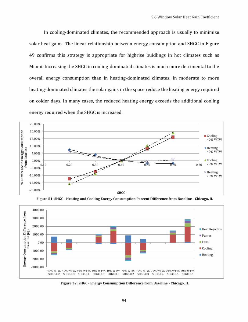
5.6 Window Solar Heat Gain Coefficient
94
In cooling-dominated climates, the recommended approach is usually to minimize
solar heat gains. The linear relationship between energy consumption and SHGC in Figure
49 confirms this strategy is appropriate for highrise buidlings in hot climates such as
Miami. Increasing the SHGC in cooling-dominated climates is much more detrimental to the
overall energy consumption than in heating-dominated climates. In moderate to more
heating-dominated climates the solar gains in the space reduce the heating energy required
on colder days. In many cases, the reduced heating energy exceeds the additional cooling
energy required when the SHGC is increased.
-3000.00
-2000.00
-1000.00
0.00
1000.00
2000.00
3000.00
4000.00
40% WTW,SHGC-0.2
40% WTW,SHGC-0.3
40% WTW,SHGC-0.4
40% WTW,SHGC-0.5
40% WTW,SHGC-0.6
70% WTW,SHGC-0.2
70% WTW,SHGC-0.3
70% WTW,SHGC-0.4
70% WTW,SHGC-0.5
70% WTW,SHGC-0.6
En
erg
y C
on
sum
pti
on
Dif
fere
nce
fro
m
Ba
seli
ne
(G
J) Heat Rejection
Pumps
Fans
Cooling
Heating
-20.00%
-15.00%
-10.00%
-5.00%
0.00%
5.00%
10.00%
15.00%
20.00%
25.00%
0.10 0.20 0.30 0.40 0.50 0.60 0.70
% D
iffe
ren
ce in
En
erg
y C
on
sum
pti
on
fr
om
Ba
seli
ne
SHGC
Cooling40% WTW
Heating40% WTW
Cooling70% WTW
Heating70% WTW
Figure 52: SHGC - Energy Consumption Difference from Baseline - Chicago, IL
Figure 51: SHGC - Heating and Cooling Energy Consumption Percent Difference from Baseline - Chicago, IL

5.6 Window Solar Heat Gain Coefficient
95
The figures for all climate zones can be seen in Appendix D These graphs show that
as the graphs move from climate zone 1A to 7, the increased SHGC becomes less
detrimental to the cooling energy consumption. In Chicago and Duluth, an increase in SHGC
beyond ASHRAE 90.1-2010 requirements results in a decrease in the amount of heating
energy required. However, because of the additional cooling energy required, the
drawbacks outweigh benefits. ASHRAE 90.1-2010 dictates a prescriptive requirement for a
maximum SHGC of 0.25 for Miami’s climate. Because not many products on the market
have SHGC’s much lower than 0.25, the opportunities to improve the energy consumption
in a highrise building beyond code requirements are limited when assessing SHGC.
Table 13: Sensitivity of Annual Energy Consumption and Cost with respect to change in SHGC
40% WTW 70% WTW
Climate Annual Energy
Change (GJ/0.1SHGC)
% Annual Energy Change (%GJ/0.1SHGC)
Annual Cost Change
($/0.1 SHGC)
% Annual Cost Change
(% $/0.1 SHGC)
Annual Energy Change
(GJ/0.1SHGC)
% Annual Energy Change (%GJ/0.1SHGC)
Annual Cost Change
($/0.1SHGC)
% Annual Cost Change
(% $/0.1 SHGC)
Miami, FL 190.49 0.28% $ 37,201.14 2.48% 204.34 0.42% $ 55,818.00 3.65%
Houston, TX 189.71 0.29% $ 44,256.86 2.47% 169.12 0.37% $ 59,253.43 3.28%
Phoenix, AZ 164.33 0.26% $ 23,112.05 1.88% 171.36 0.38% $ 42,411.71 3.32%
Atlanta, GA 173.01 0.28% $ 40,396.00 2.62% 127.55 0.31% $ 42,712.57 2.85%
San Francisco, CA 165.37 0.33% $ 49,758.57 2.52% 173.53 0.47% $ 75,115.14 3.71%
Baltimore, MD 197.34 0.31% $ 30,120.50 2.70% 91.23 0.28% $ 35,166.50 3.07%
Seattle, WA 168.28 0.32% $ 24,466.00 2.54% 130.75 0.45% $ 36,716.50 3.58%
Chicago, IL 93.35 0.15% $ 23,948.00 1.76% 71.35 0.21% $ 33,408.00 2.33%
Denver, CO 106.86 0.20% $ 10,377.50 1.98% 82.80 0.28% $ 15,610.50 2.81%
Helena, MT 79.39 0.14% $ 17,560.00 1.70% 63.95 0.22% $ 27,865.50 2.56%
Duluth, MN 23.19 0.04% $ 9,736.67 1.07% 18.42 0.08% $ 16,224.00 1.67%
While the change in energy consumption may not be large, it does have significant
implications for utility costs. Because the change of cost and energy consumption are both
approximately linear (Figures 53-56), it allows for the calculation of change from the

5.6 Window Solar Heat Gain Coefficient
96
baseline per increase of 0.1 SHGC. The values are shown in Table 13, which shows the
sensitivity of energy consumption and cost as they relate to SHGC. As pointed out earlier,
energy consumption in cooler climates is less responsive to SHGC. However, because of the
different utility rates and because cost of electricity is generally higher than gas, the
percent change in annual utility costs is relatively similar across all climates. However, the
utility cost savings achieved could justify additional costs incurred by installing a window
with a lower SHGC.
Table 14: Estimated Simple Payback Period for Reducing SHGC
Climate change
in SHGC
Increased Cost/sqft
Base Cost
Cost for “Best” SHGC
Increased cost
(40% WTW)
Annual Savings
Payback Period
Increased cost
(70% WTW)
Annual Savings
Payback Period
Miami, FL 0.05 0.409 $75.00 $75.41 $54,490 $26,871 2.03 $95,212 $32,897 2.89
Houston, TX 0.05 0.409 $75.00 $75.41 $54,490 $25,896 2.10 $95,212 $33,050 2.88
Phoenix, AZ 0.05 0.409 $75.00 $75.41 $54,490 $16,909 3.22 $95,212 $24,190 3.94
Atlanta, GA 0.05 0.409 $75.00 $75.41 $54,490 $26,144 2.08 $95,212 $22,470 4.24
San Francisco, CA 0.05 0.409 $75.00 $75.41 $54,489 $26,359 2.07 $95,212 $41,172 2.31
Baltimore, MD 0.2 1.638 $75.00 $76.64 $217,958 $36,392 5.99 $380,850 $45,705 8.33
Seattle, WA 0.2 1.638 $75.00 $76.64 $217,958 $37,266 5.85 $380,850 $57,553 6.62
Chicago, IL 0.2 1.638 $75.00 $76.64 $217,958 $32,974 6.61 $380,850 $48,903 7.79
Denver, CO 0.2 1.638 $75.00 $76.64 $217,958 $14,035 15.53 $380,850 $18,866 20.19
Helena, MT 0.2 1.638 $75.00 $76.64 $217,958 $20,951 10.40 $380,850 $31,885 11.94
Duluth, MN 0.25 2.047 $75.00 $77.05 $272,448 $15,255 17.86 $476,062 $26,477 17.98
As with the U-value, cost savings and simple payback period were calculated from
the cost information available from NREL. There are two window assemblies with the same
U-value and different SHGC. Without a detailed database that provides the exact cost of the
particular assemblies in the models, the cost must be extrapolated from the NREL data.
Simple payback periods were calculated for reducing the SHGC in each climate to 0.2. Not
surprisingly, the cooling-dominated climates show payback periods under 10 years.
However, if the real cost of decreasing the SHGC as anywhere near the $8.2/SHGC used for

5.6 Window Solar Heat Gain Coefficient
97
this estimation, then initial capital cost will be offset in a reasonable amount of time. In
combination with an optimal U-value, the payback period of the envelope improvements
would be attractive to any building owner.
0
10000
20000
30000
40000
50000
60000
70000
80000
90000
0.15 0.25 0.35 0.45 0.55 0.65
En
erg
y C
on
sum
pti
on
(G
J)
SHGC
Miami, FL
Houston, TX
Phoenix, AZ
Atlanta, GA
San Francisco, CA
Baltimore, MD
Seattle, WA
Chicago, IL
Denver, CO
Helena, MT
Duluth, MN
0
10000
20000
30000
40000
50000
60000
70000
80000
0.15 0.25 0.35 0.45 0.55 0.65
En
erg
y C
on
sum
pti
on
(G
J)
SHGC
Miami, FL
Houston, TX
Phoenix, AZ
Atlanta, GA
San Francisco, CA
Baltimore, MD
Seattle, WA
Chicago, IL
Denver, CO
Helena, MT
Duluth, MN
Figure 53: SHGC - Annual Energy Consumption vs. Solar Heat Gain Coefficient - 40% WTW Ratio
Figure 54: SHGC - Annual Energy Consumption vs. Solar Heat Gain Coefficient - 70% WTW Ratio

5.6 Window Solar Heat Gain Coefficient
98
$-
$500,000
$1,000,000
$1,500,000
$2,000,000
$2,500,000
0.15 0.25 0.35 0.45 0.55 0.65
En
erg
y C
ost
($
)
SHGC
Miami, FL
Houston, TX
Phoenix, AZ
Atlanta, GA
San Francisco, CA
Baltimore, MD
Seattle, WA
Chicago, IL
Denver, CO
Helena, MT
Duluth, MN
$-
$500,000
$1,000,000
$1,500,000
$2,000,000
$2,500,000
0.15 0.25 0.35 0.45 0.55 0.65
En
erg
y C
ost
($
)
SHGC
Miami, FL
Houston, TX
Phoenix, AZ
Atlanta, GA
San Francisco, CA
Baltimore, MD
Seattle, WA
Chicago, IL
Denver, CO
Helena, MT
Duluth, MN
Figure 55: Annual Energy Cost vs. Solar Heat Gain Coefficient - 40% WTW Ratio
Figure 56: Annual Energy Cost vs. Solar Heat Gain Coefficient - 70% WTW Ratio

5.7 Impacts of Daylight Control
99
5.7 Impacts of Daylight Control
Daylight Control is an often-used energy conservation method that involves the
installation of sensors within the space that feed a control system that keeps the
illuminance in the space at a set value. For offices a typical value is 500lux. AHSRAE 90.1-
2010 [88] now requires photocell daylighting controls when the “primary sightlighted area
in an enclosed space equals or exceeds 250ft2.” Most offices would fit this criteria, so
daylighting of exterior zones has become standard practice. Daylighting takes advantage of
useful light as it penetrates the glazing, and reduces the lighting power to meet the
illuminance setpoint of the space. While daylight control is not part of the envelope design,
variables such as window-to-wall ratio, SHGC, and overhang depth can have a major
influence on the effectiveness of daylight control. Simulations were run with added daylight
control to determine whether the addition of daylight control would impact the sensitivity
of these variables. Daylighting sensors were assigned to the center of each perimeter
façade zone at the height of the work plane, and were assigned a conservative setpoint of
500lux.
EnergyPlus offers two different daylight control calculation methodologies: Detailed
and DELight. The main differences between the two methods are that DELight can analyze
complex fenestration and shading devices, and that DELight calculates interior refelctions
with a radiosity method. There are a few other differences in the calculations, outlined in
EnergyPlus documentation. The most critical attribute to assess when selecting a
methodology is accuracy of the calcualtion. Todd Gibson performed a validation study of
several different daylighting software packages, including EnergyPlus Detailed calculations
and EnergyPlus DELight [97]. Gibson compared each software to measured experimental

5.7 Impacts of Daylight Control
100
data and found that the Detailed calculations offered a much more realistic approximation
for the illuminance on the work plane at different sensor locations, varying exterior
illuminance conditions, and did not dramatically increase simulation time. For these
reasons, the detailed method was utilized for this analysis.
By just implementing the daylight control in the baseline highrise, immediately
Miami and Chicago each experience around $50,000 annual cost savings. The NREL
Technical Support Document cites a study performed by RMH Group in 2010 that
estimated the cost of implementing daylighting controls at $0.55/ft2 of daylit area. The
capital cost of the daylight control system for this particular model is $195,275. Given the
yearly cost savings of implementing the daylighting, the payback period would be around 4
years, and well worth the initial investment.
5.7.1 Daylight Control and Window-to-wall Ratio
The response of energy cost to increased WTW ratio is very similar in the cases with
daylight control and without. Adding daylight control reduces the change in cost for each
percent of increased WTW ratio by $408/(%WTW). Chicago is even less impacted by the
addition of daylight in the WTW ratio cases, with a reduction of only $49/(%WTW).
$(20,000)
$(10,000)
$-
$10,000
$20,000
$30,000
$40,000
$50,000
$60,000
$70,000
$80,000
30% 40% 50% 60% 70% 80% 90% 100%En
erg
y C
ost
Dif
fere
nce
fro
m
Ba
seli
ne
WTW Ratio
Miami WTW
Miami WTW Daylight
Figure 57: Daylight Comparison - Energy Cost Difference from Baseline - Miami, FL
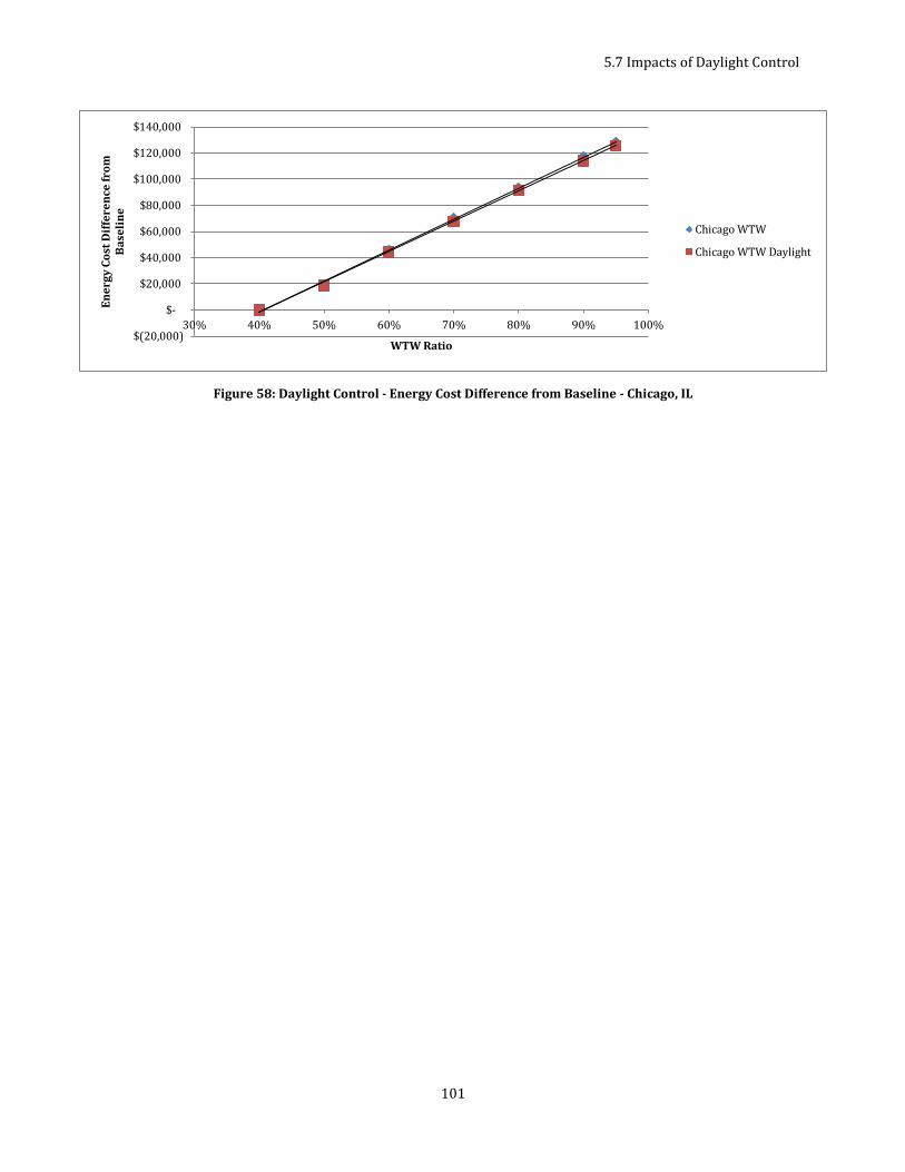
5.7 Impacts of Daylight Control
101
$(20,000)
$-
$20,000
$40,000
$60,000
$80,000
$100,000
$120,000
$140,000
30% 40% 50% 60% 70% 80% 90% 100%
En
erg
y C
ost
Dif
fere
nce
fro
m
Ba
seli
ne
WTW Ratio
Chicago WTW
Chicago WTW Daylight
Figure 58: Daylight Control - Energy Cost Difference from Baseline - Chicago, IL
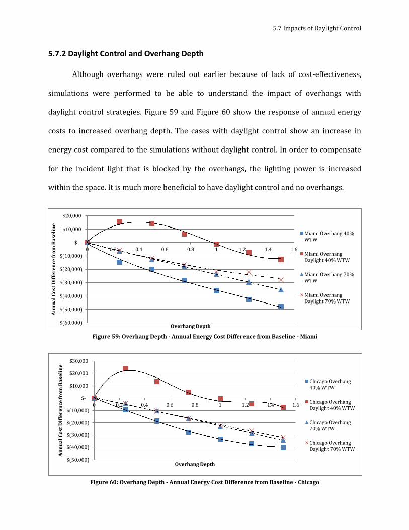
5.7 Impacts of Daylight Control
102
5.7.2 Daylight Control and Overhang Depth
Although overhangs were ruled out earlier because of lack of cost-effectiveness,
simulations were performed to be able to understand the impact of overhangs with
daylight control strategies. Figure 59 and Figure 60 show the response of annual energy
costs to increased overhang depth. The cases with daylight control show an increase in
energy cost compared to the simulations without daylight control. In order to compensate
for the incident light that is blocked by the overhangs, the lighting power is increased
within the space. It is much more beneficial to have daylight control and no overhangs.
$(60,000)
$(50,000)
$(40,000)
$(30,000)
$(20,000)
$(10,000)
$-
$10,000
$20,000
0 0.2 0.4 0.6 0.8 1 1.2 1.4 1.6
An
nu
al
Co
st D
iffe
ren
ce f
rom
Ba
seli
ne
Overhang Depth
Miami Overhang 40%WTW
Miami OverhangDaylight 40% WTW
Miami Overhang 70%WTW
Miami OverhangDaylight 70% WTW
Figure 59: Overhang Depth - Annual Energy Cost Difference from Baseline - Miami
$(50,000)
$(40,000)
$(30,000)
$(20,000)
$(10,000)
$-
$10,000
$20,000
$30,000
0 0.2 0.4 0.6 0.8 1 1.2 1.4 1.6
An
nu
al
Co
st D
iffe
ren
ce f
rom
Ba
seli
ne
Overhang Depth
Chicago Overhang40% WTW
Chicago OverhangDaylight 40% WTW
Chicago Overhang70% WTW
Chicago OverhangDaylight 70% WTW
Figure 60: Overhang Depth - Annual Energy Cost Difference from Baseline - Chicago
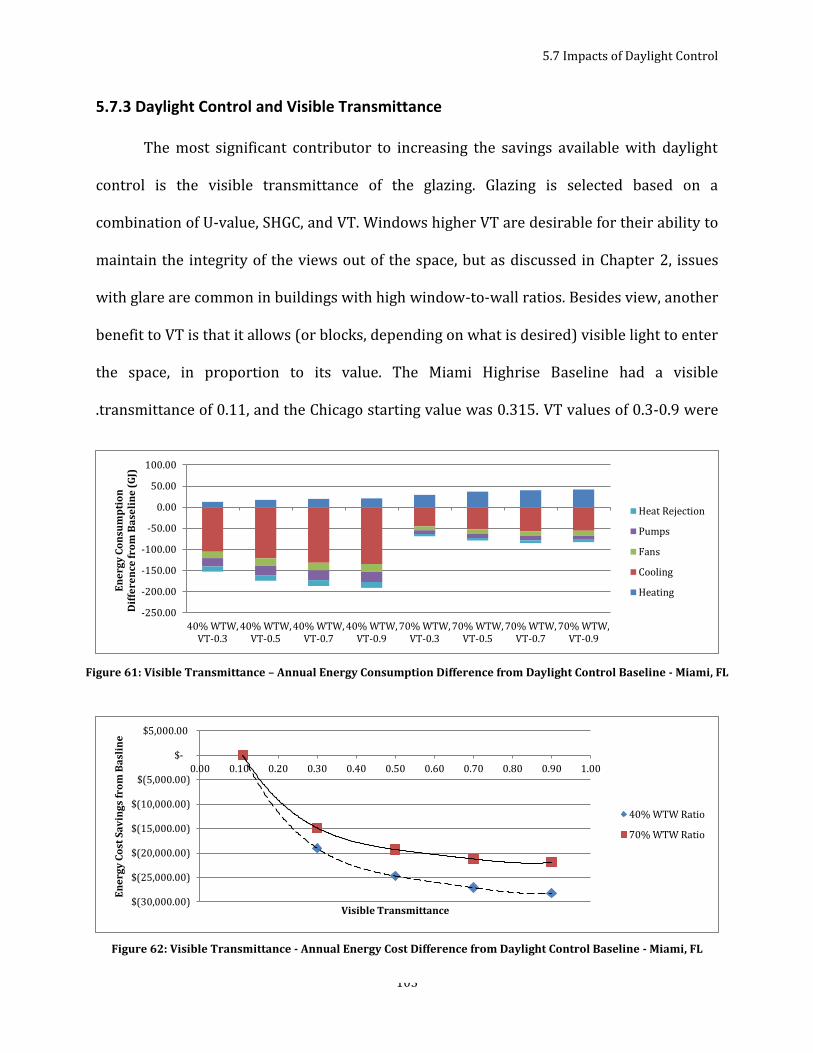
5.7 Impacts of Daylight Control
103
5.7.3 Daylight Control and Visible Transmittance
The most significant contributor to increasing the savings available with daylight
control is the visible transmittance of the glazing. Glazing is selected based on a
combination of U-value, SHGC, and VT. Windows higher VT are desirable for their ability to
maintain the integrity of the views out of the space, but as discussed in Chapter 2, issues
with glare are common in buildings with high window-to-wall ratios. Besides view, another
benefit to VT is that it allows (or blocks, depending on what is desired) visible light to enter
the space, in proportion to its value. The Miami Highrise Baseline had a visible
.transmittance of 0.11, and the Chicago starting value was 0.315. VT values of 0.3-0.9 were
$(30,000.00)
$(25,000.00)
$(20,000.00)
$(15,000.00)
$(10,000.00)
$(5,000.00)
$-
$5,000.00
0.00 0.10 0.20 0.30 0.40 0.50 0.60 0.70 0.80 0.90 1.00
En
erg
y C
ost
Sa
vin
gs
fro
m B
asl
ine
Visible Transmittance
40% WTW Ratio
70% WTW Ratio
-250.00
-200.00
-150.00
-100.00
-50.00
0.00
50.00
100.00
40% WTW,VT-0.3
40% WTW,VT-0.5
40% WTW,VT-0.7
40% WTW,VT-0.9
70% WTW,VT-0.3
70% WTW,VT-0.5
70% WTW,VT-0.7
70% WTW,VT-0.9
En
erg
y C
on
sum
pti
on
D
iffe
ren
ce f
rom
Ba
seli
ne
(G
J)
Heat Rejection
Pumps
Fans
Cooling
Heating
Figure 61: Visible Transmittance – Annual Energy Consumption Difference from Daylight Control Baseline - Miami, FL
Figure 62: Visible Transmittance - Annual Energy Cost Difference from Daylight Control Baseline - Miami, FL
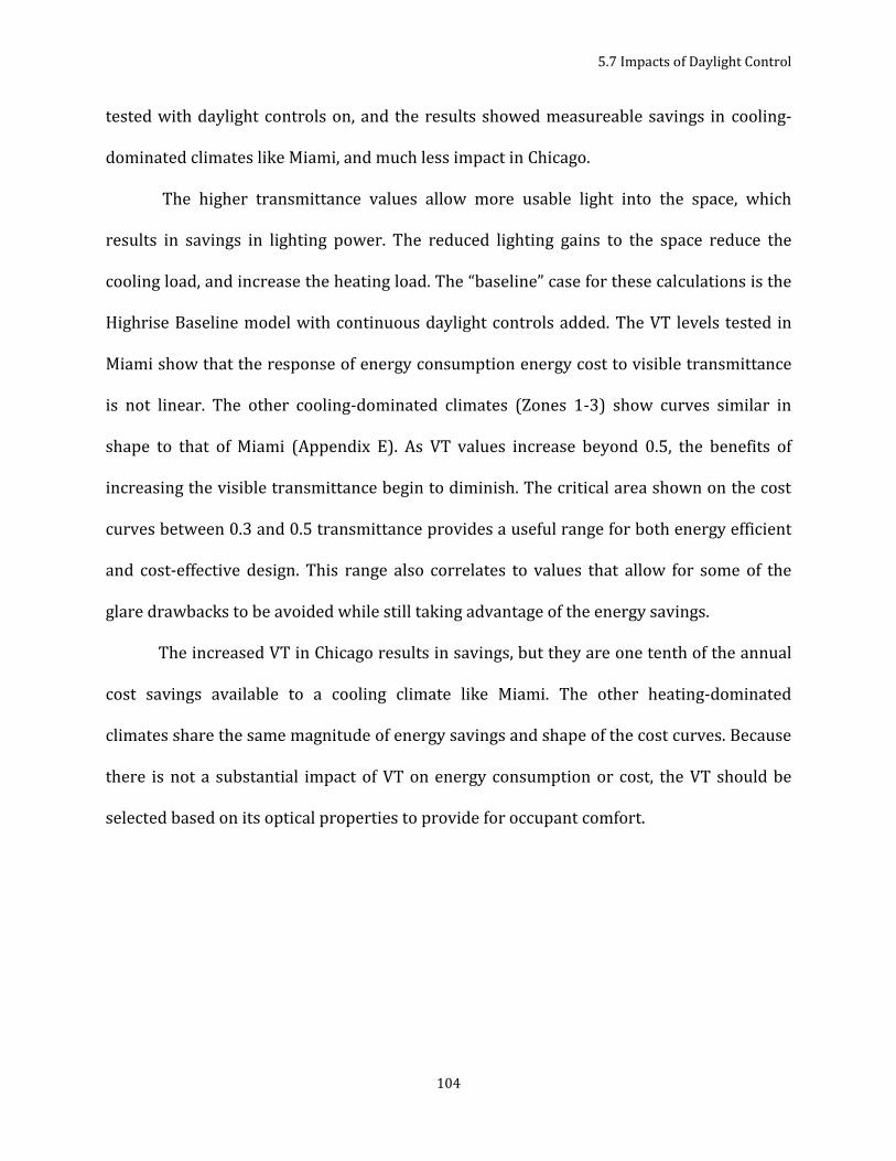
5.7 Impacts of Daylight Control
104
tested with daylight controls on, and the results showed measureable savings in cooling-
dominated climates like Miami, and much less impact in Chicago.
The higher transmittance values allow more usable light into the space, which
results in savings in lighting power. The reduced lighting gains to the space reduce the
cooling load, and increase the heating load. The “baseline” case for these calculations is the
Highrise Baseline model with continuous daylight controls added. The VT levels tested in
Miami show that the response of energy consumption energy cost to visible transmittance
is not linear. The other cooling-dominated climates (Zones 1-3) show curves similar in
shape to that of Miami (Appendix E). As VT values increase beyond 0.5, the benefits of
increasing the visible transmittance begin to diminish. The critical area shown on the cost
curves between 0.3 and 0.5 transmittance provides a useful range for both energy efficient
and cost-effective design. This range also correlates to values that allow for some of the
glare drawbacks to be avoided while still taking advantage of the energy savings.
The increased VT in Chicago results in savings, but they are one tenth of the annual
cost savings available to a cooling climate like Miami. The other heating-dominated
climates share the same magnitude of energy savings and shape of the cost curves. Because
there is not a substantial impact of VT on energy consumption or cost, the VT should be
selected based on its optical properties to provide for occupant comfort.

5.7 Impacts of Daylight Control
105
-40
-20
0
20
40
60
80
100
120
140
160
40% WTW,VT-0.3
40% WTW,VT-0.5
40% WTW,VT-0.7
40% WTW,VT-0.9
70% WTW,VT-0.3
70% WTW,VT-0.5
70% WTW,VT-0.7
70% WTW,VT-0.9
En
erg
y C
on
sum
pti
on
Dif
fere
nce
fro
m
Ba
seli
ne
(G
J) Heat Rejection
Pumps
Fans
Cooling
Heating
There is no cost data available that provides a direct relationship between VT and
cost per square foot of glazing, so no payback period can be calculated for VT. It is very
difficult to isolate any of the window parameters from the others. However, a visible
transmittance value appropriate for the climate and for the occupants clearly can provide
energy savings, cost savings, and a comfortable space.
Figure 63: Visible Transmittance - Annual Energy Consumption Difference from Daylight Control Baseline - Chicago, IL
$(4,500.00)
$(4,000.00)
$(3,500.00)
$(3,000.00)
$(2,500.00)
$(2,000.00)
$(1,500.00)
$(1,000.00)
$(500.00)
$-
$500.00
$1,000.00
0.000 0.200 0.400 0.600 0.800 1.000
En
erg
y C
ost
Sa
vin
gs
fro
m B
ase
lin
e
40% WTW Ratio
70% WTW Ratio
Figure 64: Visible Transmittance - Annual Energy Cost Difference from Daylight Control Baseline - Chicago, IL

Chapter 6: Parametric Analysis of Window Properties
106
Chapter 6: Parametric Analysis of Window Properties
6.1 Parametric Analysis of Window Properties
The sensitivity analyses in Chapter 5 provide useful insight as to which variables
have the most significant impacts on overall building energy consumption. Because of the
high window-to-wall ratio and the more critical energy path in the walls of the glazing,
annual energy consumption and cost were not very sensitive to changes in the wall U-
values for a highrise building with a curtainwall construction. The analysis of the
adjustment of WTW ratio showed that setting a maximum WTW ratio of 50% is beneficial
for all climates, and limiting it to 40% is beneficial in all climate zones “higher” than climate
zone 3A. Although the argument for limiting WTW ratio for the purposes of limiting energy
consumption is compelling, there are tradeoffs such as view and aesthetics to consider.
These are a few of the driving factors that have led to WTW ratios more typically around
70% in current high-rise buildings. Overhangs are typically cost-prohibitive in highrise
building design, although they do result in reduced energy consumption. Window U-value,
SHGC, VT, and daylighting controls had the greatest energy consumption impacts, and
made the most compelling economic cases as well.

6.1 Parametric Analysis of Window Properties
107
Chapter 5 showed that the critical highrise wall properties are the glazing
properties. Therefore, a more thorough analysis of curtainwall performance focused on the
glazing properties was performed. When selecting glazing for an assembly, all three
window properties must be specified: U-value, SHGC, and VT. While the Chapter 5 analyses
held all variables constant except for the variable of interest, in real-world applications all
three window properties are subject to change. In order to understand the interaction
between the three properties, a parametric analysis was performed.
The WTW ratio for the parametric analysis was held constant at 70% WTW ratio, to
represent a typical WTW ratio for current curtainwall designs. Daylighting was modeled (at
a 500 lux setpoint) because it has become standard practice, and in many jurisdictions,
required by code. Enabling daylighting controls of the interior lighting also allows for a
better understanding of all the energy tradeoffs possible via adjusting the window
properties. Overhangs were not modeled in light of the high initial cost of incorporating
them into the design.
The parametric analysis was performed in all climate zones previously assessed,
and the following window properties were analyzed:
Table 15: Window Properties for Parametric Analysis
U-value SHGC VT
0.08 0.1 0.3
0.2 0.2 0.5
0.4 0.3 0.7
0.6 0.4 0.9
0.8 0.5
0.6
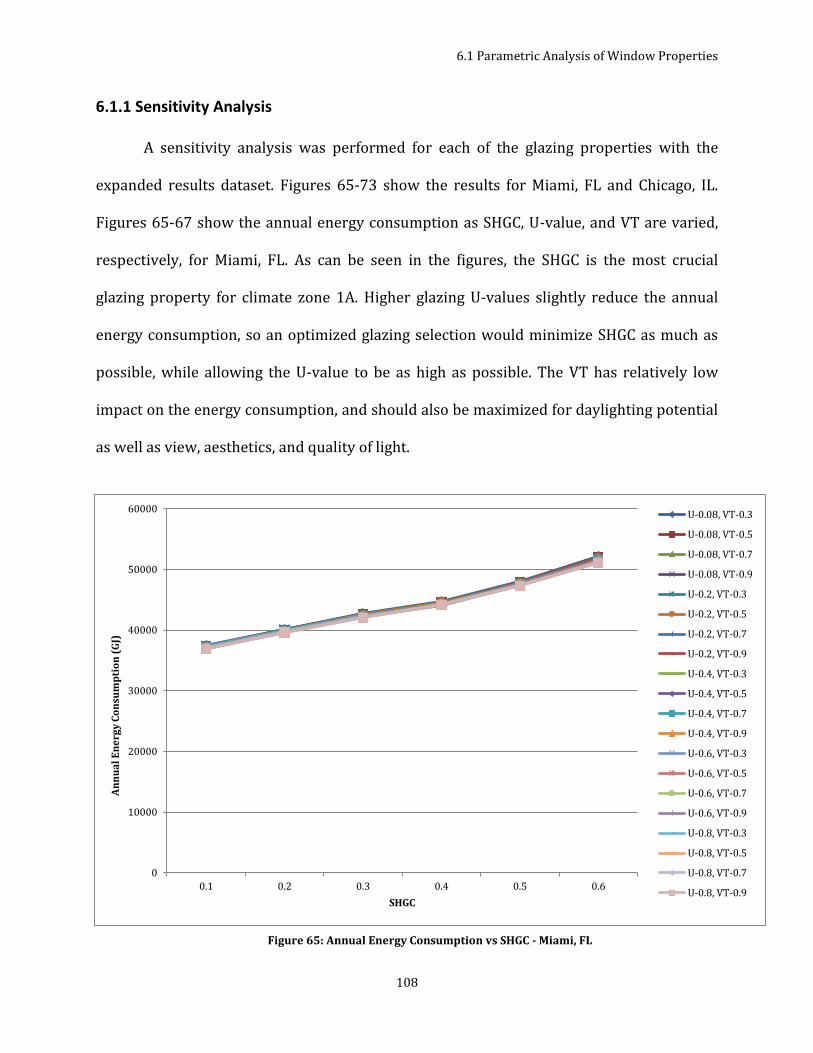
6.1 Parametric Analysis of Window Properties
108
6.1.1 Sensitivity Analysis
A sensitivity analysis was performed for each of the glazing properties with the
expanded results dataset. Figures 65-73 show the results for Miami, FL and Chicago, IL.
Figures 65-67 show the annual energy consumption as SHGC, U-value, and VT are varied,
respectively, for Miami, FL. As can be seen in the figures, the SHGC is the most crucial
glazing property for climate zone 1A. Higher glazing U-values slightly reduce the annual
energy consumption, so an optimized glazing selection would minimize SHGC as much as
possible, while allowing the U-value to be as high as possible. The VT has relatively low
impact on the energy consumption, and should also be maximized for daylighting potential
as well as view, aesthetics, and quality of light.
Figure 65: Annual Energy Consumption vs SHGC - Miami, FL
0
10000
20000
30000
40000
50000
60000
0.1 0.2 0.3 0.4 0.5 0.6
An
nu
al
En
erg
y C
on
sum
pti
on
(G
J)
SHGC
U-0.08, VT-0.3
U-0.08, VT-0.5
U-0.08, VT-0.7
U-0.08, VT-0.9
U-0.2, VT-0.3
U-0.2, VT-0.5
U-0.2, VT-0.7
U-0.2, VT-0.9
U-0.4, VT-0.3
U-0.4, VT-0.5
U-0.4, VT-0.7
U-0.4, VT-0.9
U-0.6, VT-0.3
U-0.6, VT-0.5
U-0.6, VT-0.7
U-0.6, VT-0.9
U-0.8, VT-0.3
U-0.8, VT-0.5
U-0.8, VT-0.7
U-0.8, VT-0.9

6.1 Parametric Analysis of Window Properties
109
0
10000
20000
30000
40000
50000
60000
0.08 0.2 0.4 0.6 0.8
An
nu
al
En
erg
y C
on
sum
pti
on
(G
J)
U-value
SHGC-0.1, VT-0.3
SHGC-0.1, VT-0.5
SHGC-0.1, VT-0.7
SHGC-0.1, VT-0.9
SHGC-0.2, VT-0.3
SHGC-0.2, VT-0.5
SHGC-0.2, VT-0.7
SHGC-0.2, VT-0.9
SHGC-0.3, VT-0.3
SHGC-0.3, VT-0.5
SHGC-0.3, VT-0.7
SHGC-0.3, VT-0.9
SHGC-0.4, VT-0.3
SHGC-0.4, VT-0.5
SHGC-0.4, VT-0.7
SHGC-0.4, VT-0.9
SHGC-0.5, VT-0.3
SHGC-0.5, VT-0.5
SHGC-0.5, VT-0.7
SHGC-0.5, VT-0.9
SHGC-0.6, VT-0.3
SHGC-0.6, VT-0.5
SHGC-0.6, VT-0.7
SHGC-0.6, VT-0.9
Figure 66: Annual Energy Consumption vs. U-value – Miami,FL
0
10000
20000
30000
40000
50000
60000
0.3 0.5 0.7 0.9
An
nu
al
En
erg
y C
on
sum
pti
on
(G
J)
Visible Transmittance
U-0.08, SHGC-0.1U-0.08, SHGC-0.2U-0.08, SHGC-0.3U-0.08, SHGC-0.4U-0.08, SHGC-0.5U-0.08, SHGC-0.6U-0.2, SHGC-0.1U-0.2, SHGC-0.2U-0.2, SHGC-0.3U-0.2, SHGC-0.4U-0.2, SHGC-0.5U-0.2, SHGC-0.6U-0.4, SHGC-0.1U-0.4, SHGC-0.2U-0.4, SHGC-0.3U-0.4, SHGC-0.4U-0.4, SHGC-0.5U-0.4, SHGC-0.6U-0.6, SHGC-0.1U-0.6, SHGC-0.2U-0.6, SHGC-0.3U-0.6, SHGC-0.4U-0.6, SHGC-0.5U-0.6, SHGC-0.6U-0.8, SHGC-0.1U-0.8, SHGC-0.2U-0.8, SHGC-0.3U-0.8, SHGC-0.4U-0.8, SHGC-0.5U-0.8, SHGC-0.6
Figure 67: Annual Energy Consumption vs. Visible Transmittance - Miami, FL

6.1 Parametric Analysis of Window Properties
110
Figure 68 shows how the components of HVAC energy are impacted as the SHGC is
increased for a U-value of 0.2 and a VT of 50%. The required cooling energy is the HVAC
component most heavily impacted by the increase in SHGC. End uses also tied to cooling
energy such as heat rejection, pumps, and fans also increase in annual energy consumption
as the SHGC is increased. The graphs for other combinations of U-value and VT follow
similar trends.
Figures 69-71 show the same information for Chicago, IL. As the results of the
Chapter 5 analyses showed, the building energy consumption for a building in climate zone
5A is much more responsive to changes in U-value than the warmer climate of Miami. The
slope of the SHGC graph as compared to the U-value graph shows that the building energy
consumption is marginally more sensitive to SHGC than U-value. However, both variables
are critical to the optimization of energy consumption for heating-dominated climates. For
an optimal glazing selection for Chicago, the U-value and SHGC should both be minimized.
The VT also has relatively little impact, and should be maximized.
0
10000
20000
30000
40000
50000
60000
0.1 0.2 0.3 0.4 0.5 0.6
An
nu
al
En
d U
se E
ne
rgy
Co
nsu
mp
tio
n (
GJ)
SHGC
Sum of Heat Rejection
Sum of Pumps
Sum of Fans
Sum of Interior Lighting
Sum of Heating
Sum of Cooling
Figure 68: Annual End Use Energy Consumption vs. SHGC - Miami, FL - U-0.2, VT 50%

6.1 Parametric Analysis of Window Properties
111
0
5000
10000
15000
20000
25000
30000
35000
40000
0.08 0.2 0.4 0.6 0.8
An
nu
al
En
erg
y C
on
sum
pti
on
(G
J)
U-value
SHGC-0.1, VT-0.3
SHGC-0.1, VT-0.5
SHGC-0.1, VT-0.7
SHGC-0.1, VT-0.9
SHGC-0.2, VT-0.3
SHGC-0.2, VT-0.5
SHGC-0.2, VT-0.7
SHGC-0.2, VT-0.9
SHGC-0.3, VT-0.3
SHGC-0.3, VT-0.5
SHGC-0.3, VT-0.7
SHGC-0.3, VT-0.9
SHGC-0.4, VT-0.3
SHGC-0.4, VT-0.5
SHGC-0.4, VT-0.7
SHGC-0.4, VT-0.9
SHGC-0.5, VT-0.3
SHGC-0.5, VT-0.5
SHGC-0.5, VT-0.7
SHGC-0.5, VT-0.9
SHGC-0.6, VT-0.3
SHGC-0.6, VT-0.5
SHGC-0.6, VT-0.7
SHGC-0.6, VT-0.9
0
5000
10000
15000
20000
25000
30000
35000
40000
0.1 0.2 0.3 0.4 0.5 0.6
An
nu
al
En
erg
y C
on
sum
pti
on
(G
J)
SHGC
U-0.08, VT-0.3
U-0.08, VT-0.5
U-0.08, VT-0.7
U-0.08, VT-0.9
U-0.2, VT-0.3
U-0.2, VT-0.5
U-0.2, VT-0.7
U-0.2, VT-0.9
U-0.4, VT-0.3
U-0.4, VT-0.5
U-0.4, VT-0.7
U-0.4, VT-0.9
U-0.6, VT-0.3
U-0.6, VT-0.5
U-0.6, VT-0.7
U-0.6, VT-0.9
U-0.8, VT-0.3
U-0.8, VT-0.5
U-0.8, VT-0.7
U-0.8, VT-0.9
Figure 69: Annual Energy Consumption vs. SHGC – Chicago, IL
Figure 70: Annual Energy Consumption vs. U-value – Chicago, IL

6.1 Parametric Analysis of Window Properties
112
Figure 72 shows how the components of HVAC energy are impacted as the SHGC is
increased for a U-value of 0.2 and a VT of 50%. The graphs for other U-value and VT
combinations follow similar patterns. As can be seen, the heating energy component
reaches a minimum at a SHGC of 0.3, while overall energy consumption is optimized at
0
5000
10000
15000
20000
25000
30000
35000
40000
0.3 0.5 0.7 0.9
An
nu
al
En
erg
y C
on
sum
pti
on
(G
J)
Visible Transmittance
U-0.08, SHGC-0.1U-0.08, SHGC-0.2U-0.08, SHGC-0.3U-0.08, SHGC-0.4U-0.08, SHGC-0.5U-0.08, SHGC-0.6U-0.2, SHGC-0.1U-0.2, SHGC-0.2U-0.2, SHGC-0.3U-0.2, SHGC-0.4U-0.2, SHGC-0.5U-0.2, SHGC-0.6U-0.4, SHGC-0.1U-0.4, SHGC-0.2U-0.4, SHGC-0.3U-0.4, SHGC-0.4U-0.4, SHGC-0.5U-0.4, SHGC-0.6U-0.6, SHGC-0.1U-0.6, SHGC-0.2U-0.6, SHGC-0.3U-0.6, SHGC-0.4U-0.6, SHGC-0.5U-0.6, SHGC-0.6U-0.8, SHGC-0.1U-0.8, SHGC-0.2U-0.8, SHGC-0.3U-0.8, SHGC-0.4U-0.8, SHGC-0.5U-0.8, SHGC-0.6
Figure 71: Annual Energy Consumption vs. Visible Transmittance – Chicago, IL
0
5000
10000
15000
20000
25000
30000
35000
0.1 0.2 0.3 0.4 0.5 0.6
An
nu
al
En
d U
se E
ne
rgy
Co
nsu
mp
tio
n (
GJ)
SHGC
Sum of Heat Rejection
Sum of Pumps
Sum of Fans
Sum of Interior Lighting
Sum of Heating
Sum of Cooling
Figure 72: Annual End Use Energy Consumption vs. SHGC – Chicago, IL - U-0.2, VT 50%

6.1 Parametric Analysis of Window Properties
113
minimum SHGC values. The reduction in heating energy from a SHGC of 0.1 to 0.3 is offset
by the increase in cooling energy.
Figure 73 shows a similar graph, but versus U-value on the x-axis. The cooling
energy is decreased slightly as the U-value increases. However, the driving factor for the
reduced energy consumption at lower U-values is because of the decrease in heating
energy required to overcome the conductance losses through the glazing.
Figur
6.1.2 Energy Consumption Optimization
The goal of the final analysis was to identify the optimal glazing selection for a
curtainwall assembly in each climate zone. A total of 120 simulations were run for each
climate zone, analyzing each possible combination of the glazing properties listed in Table
15. An important factor in the optimization of the glazing selection is the real-world limit
on luminous efficacy. As discussed in Section 2.3.1 Tinted Glazing, the limits to luminous
efficacy (ratio of visible transmittance to shading coefficient) determined by LBNL are 0.5
0
5000
10000
15000
20000
25000
30000
35000
0.08 0.2 0.4 0.6 0.8
An
nu
al
En
d U
se E
ne
rgy
Co
nsu
mp
tio
n (
GJ)
U-value
Sum of Heat Rejection
Sum of Pumps
Sum of Fans
Sum of Interior Lighting
Sum of Heating
Sum of Cooling
Figure 73: Annual End Use Energy Consumption vs. U-value - Chicago, IL - SHGC-0.2, VT 50%
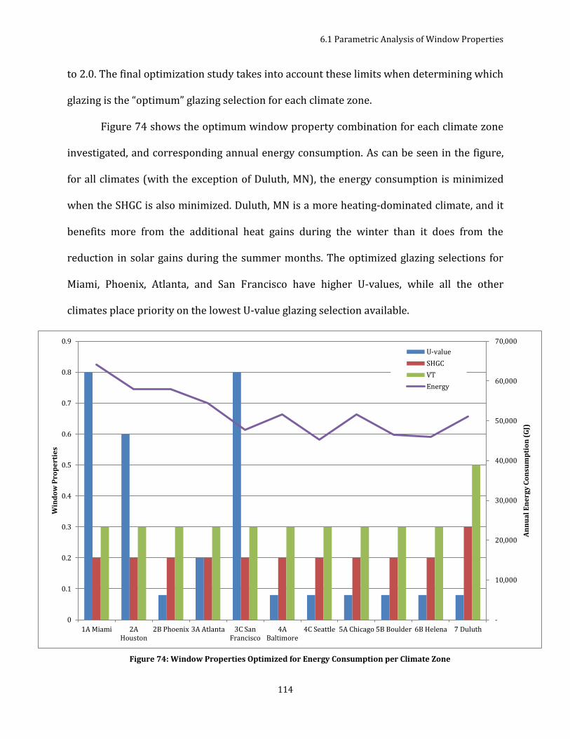
6.1 Parametric Analysis of Window Properties
114
to 2.0. The final optimization study takes into account these limits when determining which
glazing is the “optimum” glazing selection for each climate zone.
Figure 74 shows the optimum window property combination for each climate zone
investigated, and corresponding annual energy consumption. As can be seen in the figure,
for all climates (with the exception of Duluth, MN), the energy consumption is minimized
when the SHGC is also minimized. Duluth, MN is a more heating-dominated climate, and it
benefits more from the additional heat gains during the winter than it does from the
reduction in solar gains during the summer months. The optimized glazing selections for
Miami, Phoenix, Atlanta, and San Francisco have higher U-values, while all the other
climates place priority on the lowest U-value glazing selection available.
-
10,000
20,000
30,000
40,000
50,000
60,000
70,000
0
0.1
0.2
0.3
0.4
0.5
0.6
0.7
0.8
0.9
1A Miami 2AHouston
2B Phoenix 3A Atlanta 3C SanFrancisco
4ABaltimore
4C Seattle 5A Chicago 5B Boulder 6B Helena 7 Duluth
An
nu
al
En
erg
y C
on
sum
pti
on
(G
J)
Win
do
w P
rop
ert
ies
U-value
SHGC
VT
Energy
Figure 74: Window Properties Optimized for Energy Consumption per Climate Zone

6.1 Parametric Analysis of Window Properties
115
Investigated more closely, it becomes clear that for the cooling-dominated climates,
the SHGC is by far the most critical value in terms of energy efficiency. Figures 228-238 in
Appendix F show the glazing properties of the ten lowest and the ten highest energy
consumers for each climate zone. For climate zones 1A through 4C, the SHGC is the
dominant window property, and there is very little increase in annual energy consumption
(<1%) for any U-value when the SHGC and VT are minimized at 0.2 and 0.3, respectively. In
climates 5A and above, the U-value begins to play a more critical role. However the lowest
ten energy performers are all within 4% of the “optimum” glazing selection.
6.1.3 Energy Cost Optimization
In addition to weather differences across the climate zones, each climate zone has
its own utility rate structure. Consumption charges vary between utility providers, as well
as demand charges. The glazing selections not only affect annual energy consumption, but
varying the glazing properties can also raise, lower, or shift the time and magnitude of the
peak demand. For this reason, an “optimum selection” was investigated on a cost basis.
Figure 75 below shows the window properties optimized on a cost basis for all climate
zones investigated. The climate zones of Miami, San Francisco, Baltimore, Chicago, and
Helena showed no change from the energy consumption optimization. The other climate
zones (Houston, Phoenix, Atlanta, Seattle, Denver, and Duluth) had a different optimum
selection when optimizing for cost.

6.1 Parametric Analysis of Window Properties
116
While in most of these climate zones, optimizing for energy cost rather than energy
consumption results in less than 1% difference in annual energy costs, the impacts for
Duluth were more substantial. When seeking to minimize energy consumption, the
optimum glazing selection is a glazing with U-0.08, SHGC-0.3, and VT-50%. By optimizing
for cost rather than energy consumption, the optimum selection is a glazing with U-0.08,
SHGC-0.2, and VT-30%. This change in window properties reduced the annual energy cost
by $9,739 (1.2%). However, the most substantial potential cost savings for Duluth is tied to
a potential reduction in required chiller capacity by 211 tons. This is due to the reduced
$-
$200,000
$400,000
$600,000
$800,000
$1,000,000
$1,200,000
$1,400,000
$1,600,000
$1,800,000
$2,000,000
0
0.1
0.2
0.3
0.4
0.5
0.6
0.7
0.8
0.9
1A Miami 2AHouston
2BPhoenix
3A Atlanta 3C SanFrancisco
4ABaltimore
4C Seattle 5A Chicago 5B Denver 6B Helena 7 Duluth
An
nu
al
En
erg
y C
ost
($
)
Win
do
w P
rop
ert
ies
U-value
SHGC
VT
Cost
Figure 75: Window Properties Optimized for Energy Cost per Climate Zone

6.1 Parametric Analysis of Window Properties
117
SHGC and VT, which reduces the incident solar radiation, thereby reducing the peak cooling
loads in each of the exterior zones.
Each of the climate zones achieve the optimum energy cost point at minimum SHGC
and VT levels. Because electricity is generally more expensive per unit of energy across all
the climate zones, measures that reduce electricity consumption and demand have greater
impacts on annual energy costs than those that reduce natural gas consumption. As
discussed in the sensitivity analysis, the annual energy consumption of the facility is highly
sensitive to SHGC selection. Because of the relatively higher cost of electricity, and the
ability of the SHGC to minimize the peak cooling loads within the exterior zones, reducing
the SHGC is essential to minimizing the annual energy costs of the facility.
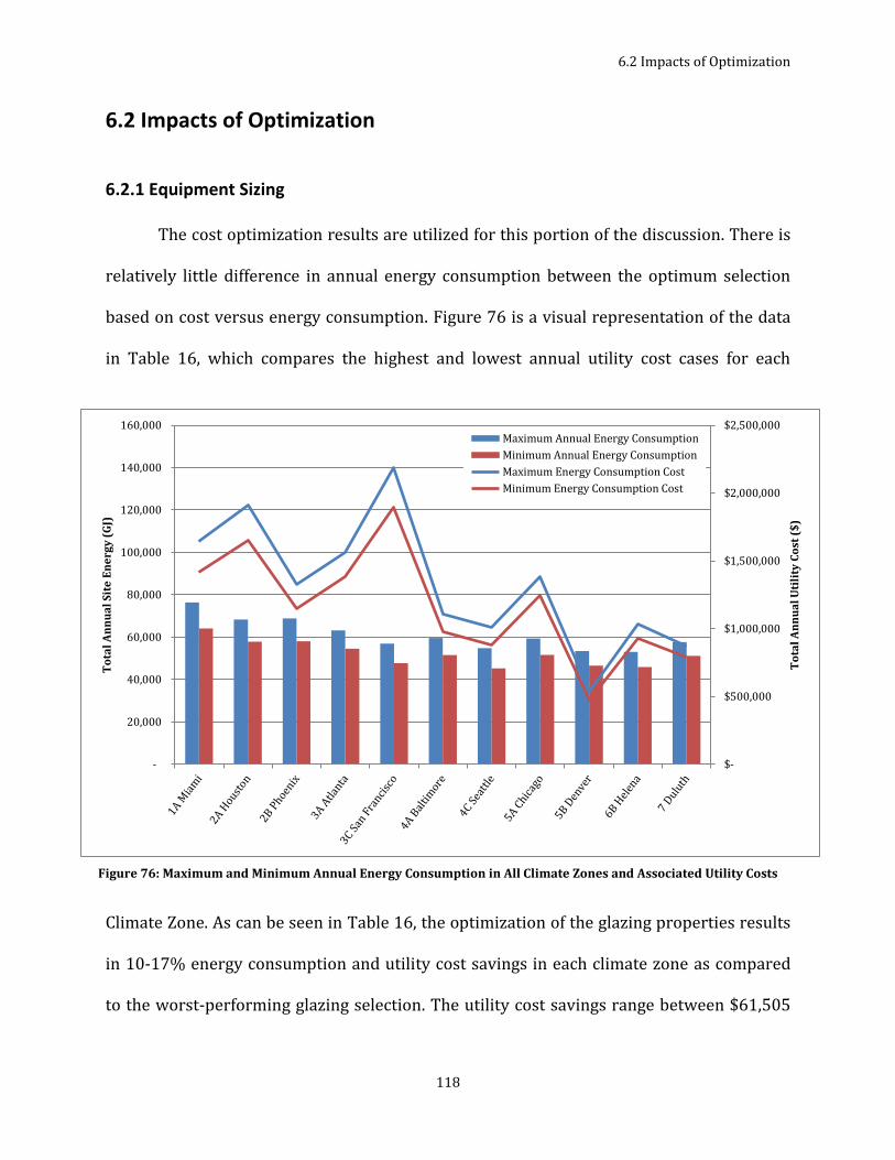
6.2 Impacts of Optimization
118
6.2 Impacts of Optimization
6.2.1 Equipment Sizing
The cost optimization results are utilized for this portion of the discussion. There is
relatively little difference in annual energy consumption between the optimum selection
based on cost versus energy consumption. Figure 76 is a visual representation of the data
in Table 16, which compares the highest and lowest annual utility cost cases for each
Climate Zone. As can be seen in Table 16, the optimization of the glazing properties results
in 10-17% energy consumption and utility cost savings in each climate zone as compared
to the worst-performing glazing selection. The utility cost savings range between $61,505
$-
$500,000
$1,000,000
$1,500,000
$2,000,000
$2,500,000
-
20,000
40,000
60,000
80,000
100,000
120,000
140,000
160,000
To
tal
An
nu
al
Uti
lity
Co
st (
$)
To
tal
An
nu
al
Sit
e E
ne
rgy
(G
J)
Maximum Annual Energy Consumption
Minimum Annual Energy Consumption
Maximum Energy Consumption Cost
Minimum Energy Consumption Cost
Figure 76: Maximum and Minimum Annual Energy Consumption in All Climate Zones and Associated Utility Costs

6.2 Impacts of Optimization
119
annual all the way up to $303,389. Each of the “maximum” glazing selections has glazing
with SHGC-0.6 and VT-50%. Glazing with similar properties is available on today’s market,
so it is a realistic option for building owners and designers.
Table 16: Maximum and Minimum Annual Energy Consumption and Associated Utility Costs
Annual Energy Consumption Annual Utility Costs
Max (GJ)
Min (GJ) Diff. % Diff,
Max ($)
Min ($) Diff. % Diff,
1A Miami 76,399 64,094 12,305 16.1% $1,644,600 $1,415,989 $228,612 13.9%
2A Houston 68,349 57,895 10,453 15.3% $1,909,846 $1,653,099 $256,747 13.4%
2B Phoenix 68,780 58,033 10,747 15.6% $1,324,483 $1,150,214 $174,268 13.2%
3A Atlanta 63,021 54,689 8,331 13.2% $1,569,372 $1,375,972 $193,400 12.3%
3C San Fran 56,392 47,695 8,697 15.4% $2,196,348 $1,892,959 $303,389 13.8%
4A Baltimore 59,591 51,554 8,037 13.5% $1,107,754 $975,399 $132,355 11.9%
4C Seattle 54,808 45,406 9,402 17.2% $1,011,470 $880,766 $130,704 12.9%
5A Chicago 59,387 51,614 7,773 13.1% $1,379,393 $1,242,364 $137,029 9.9%
5B Denver 53,459 46,596 6,864 12.8% $534,771 $473,265 $61,506 11.5%
6A Helena 53,048 45,947 7,101 13.4% $1,037,959 $929,719 $108,240 10.4%
7 Duluth 57,713 51,159 6,554 11.4% $870,502 $783,585 $86,916 10.0%
In addition to the annual energy consumption and utility cost implications
associated with an optimized glazing selection, as previously discussed, the glazing
properties are closely tied to the magnitude of the internal gains within the space and
thereby the sizing of the HVAC equipment. Table 16: Maximum and Minimum Annual
Energy Consumption and Associated Utility Costs shows the resulting differential in
calculated chiller and boiler capacities for the worst-case versus optimum glazing
selections analyzed.
The difference in chiller capacity from the worst-case glazing to the optimum
glazing selection ranges between 550 tons in and 790 tons across the climate zones. Based
on a typical cost per ton for a centrifugal chiller ($250/ton), the glazing optimization would
result in initial chiller equipment cost savings between $137,500 and $197,500 [94]. This is
a conservative estimate, as additional capital savings would be available by way of reduced

6.2 Impacts of Optimization
120
pump and piping sizing, and smaller cooling tower capacity. If the improved glazing results
in the ability to eliminate an entire chiller from the design, the mechanical room square
footage could be reduced and labor and building automation controls installation costs
would also be reduced. According to a white paper published by the International District
Energy Association, the total installed cost of a chilled water system of this size is
$3,000/ton [95]. Given this figure, the initial cost savings could be in the realm of $750,000
to $2,270,000 for the chilled water system alone.
The difference in boiler capacity ranges between 22 MBH (million Btu/hr) in Miami
and 33 MBH in San Francisco. According to a DOE study of installed cost for natural-gas-
fired hot-water boilers, this translates to initial cost savings in the range of $61,808 to
$91,376 [96]. The savings for the initial hot water system costs are similar in nature to
0
5
10
15
20
25
30
35
40
45
50
-
100
200
300
400
500
600
700
800
900
Bo
ile
r C
ap
aci
ty (
MB
H)
Ch
ile
r C
ap
aci
ty (
ton
s)
Difference in Chiller Capacity
Difference in Boiler Capacity
Figure 77: Reduction in Chiller and Boiler Capacity for Glazing Optimization

6.2 Impacts of Optimization
121
those of the chilled water system: reduced boiler size, piping, pumps, mechanical room, and
labor.
6.2.2 Occupant Comfort
Occupant comfort is a crucial function of the building’s HVAC system. However the
glazing properties play a crucial role in occupant comfort as well. EnergyPlus is able to
calculate the total time throughout the occupied hours of the year in which the HVAC
system fails to meet the operative temperature setpoint in each zone (Based on ASHRAE
55-2004). Figure 78 shows the total facility unmet cooling and heating hours (during
-
200
400
600
800
1,000
1,200
Un
me
t H
ou
rs
Max Energy Cooling Load Not Met
Max Energy Heating Load Not Met
Min Energy Cooling Load Not Met
Min Energy Heating Load Not Met
Figure 78: Unmet Cooling and Heating Hours for Maximum and Minimum Glazing Selections

6.2 Impacts of Optimization
122
occupied hours) for glazing selection with the highest and lowest energy consumption. This
was investigated to verify that energy savings were not being achieved at the expense of
occupant comfort. As shown in the graph, the glazing with the poorest energy performance
actually has greater unmet hours than the optimum selection.
A detailed investigation of the source of the unmet cooling hours reveals that the
vast majority of the unmet hours throughout the year occur in the south-facing zones
throughout the building from 1:00pm to 5:00pm. The inability of the HVAC system to
maintain the space temperature setpoint stems from the direct solar gains of the southern
façade. The space temperature rises no more than 3degC above setpoint, but does result in
unmet hours throughout the year. The simulations with lower SHGC and VT limit the direct
solar gains within the south zones, thereby reducing hours throughout the year in which
the temperature rises above setpoint.
The investigation of the unmet cooling and heating hours for the parametric
analysis results reveal a side benefit of optimizing the glazing selection for energy
performance. Glazing selections that minimize glare and reduce the peak heating and
cooling loads also offer occupants a more consistent and comfortable operative
temperature. In highrise buildings where floors are often leased to tenants, occupant
comfort is critical, and should be factored into curtainwall glazing selections.

6.2 Impacts of Optimization
123
6.2.3 Aesthetic and View Quality
While reducing SHGC and VT is a cost-effective strategy across all climate zones,
there are aesthetic and view-quality trade-offs that would need to be assessed by the
building owner and design team. In order to achieve SHGC-0.2 and VT-30%, the glazing
must be highly reflective and tinted. Below are images from the glazing manufacturer
Viracon that show the aesthetic quality of glazing walls with SHGC-0.2 and VT-30% [93].
From the occupant’s perspective, the daylight transmitted to the space will appear slightly
dim. This may be advantageous to the use of the space and desirable to the owner.
However, if natural light aesthetic and aggressive daylighting controls are high priorities
for the owner and design team, this glazing selection methodology may not represent the
“optimum” selection for the project. If a higher SHGC and VT are desired for aesthetic
purposes, the design team must also be sure to understand the energy consumption, utility
cost, and equipment sizing implications of moving away from selecting a less-than-
optimum glazing selection.
Figure 79: Viracon Glazing Examples: SHGC-0.2, VT-30% [93]

Chapter 7: Results
124
Chapter 7: Results
7.1 Design Recommendations
The analysis of the selected envelope parameters provides valuable insight into the
nature of energy consumption within a highrise building, and what efforts should be made
to improve the energy consumption of the building. For the curtainwall configuration
analyzed for this study, with a window-to-wall ratio of 70%, the difference in energy
consumption between the best- and worst-performing selections varies between 11.4%
and 17.2% in all climate zones. Given the magnitude of potential impact to energy
consumption, the optimization of curtainwall glazing properties should be a top priority for
design teams in all climate zones.
The relative difference in annual utility cost between the best- and worst-
performing selections varies between 9.9% and 13.9% in all climate zones. The annual
utility cost difference ranges between $61,505 and $303,389. The true cost impact for an
optimized glazing selection must also include the cost impacts of reduced equipment sizing.
The parametric analysis revealed substantial differences in the building’s peak heating and
cooling loads over the range of glazing property combinations. Optimizing the glazing

7.2 Summary and Future Work
125
showed potential to impact the chilled and hot water system sizing by 20-33% across the
climate zones. The savings available through reduced HVAC equipment sizing could
contribute greatly to the potential added cost of improved glazing, and should be factored
in the glazing selection cost analysis for any project.
The sensitivity and parametric analyses show that the most critical glazing property
for curtainwall designs in highrise buildings is the SHGC of the glazing. Across all climate
zones, the most efficient glazing selection minimizes SHGC, while maximizing the VT. While
this glazing selection may not possess the design team’s desired aesthetic or daylighting
characteristics, it is the most efficient glazing selection.
One of the most compelling components of the results of this study is the degree to
which the glazing selection has the ability to affect the annual energy consumption, annual
utility cost, and initial HVAC equipment sizing across all climates. It is said that the most
efficient building is one with no windows, no doors, no lights and no people. However,
because the built environment is one in which people live, work, and play, there will always
be tradeoffs between energy consumption, aesthetics, and occupant comfort. The results of
this study show that careful consideration should be made when analyzing those tradeoffs
and selecting a glazing for curtainwalls in highrise buildings. Whole building energy
modeling can be extremely useful in helping building owners and architects to assess and
understand the full impacts of the tradeoffs in glazing selection.
7.2 Summary and Future Work
Natural ventilation within a highrise building was identified as an energy efficiency
measure in Chapter 2, but was not within the scope for this research. It would be

7.2 Summary and Future Work
126
meaningful to understand the effectiveness of natural ventilation within highrise buildings
and determine the cost tradeoff between the energy saved and the additional cost for an
operational envelope.
The daylighting controls assessed in this study represented a very basic daylighting
strategy. Daylighting design is a complex process, and requires extensive modeling efforts
to optimize the design characteristics of the space. A next step in assessing the optimization
of curtainwall glazing properties in combination with daylighting would require a detailed
daylighting study. For a particular project, the team may want to analyze specific glazing
assemblies, complete with spectral properties and utilize the EnergyPlus complex glazing
system calculations. With a relatively low surface area to volume ratio, the geometry of the
DOE benchmark building does not maximize daylighting potential for a building of this size.
There are a variety of variables that could be assessed such as internal surface reflectance,
interior geometry (light shelves, open plenum design, and internal glazing), surface to
volume ratio, and footprint geometry that could be analyzed to determine whether
daylighting controls could be better utilized for a building of this size. In this study, the
visible transmittance properties of the glazing may become more critical to the overall
efficiency of the building.
Improved glazing and energy efficient curtain wall assemblies continue to be a large
focus in research. Many of the glazing strategies identified in Chapter 2 were eliminated
from this analysis because they were either too expensive to implement at current market
price, or they were too complicated for the large façade sizes associated with highrise
buildings. Continued research in both the glazing portion and the curtain wall assemblies
could potentially open up opportunities for significant energy savings in the future.

7.3 Conclusion
127
7.3 Conclusion
The preceding study shows the importance of critically assessing glazing properties
in curtainwall designs for highrise buildings. It also underscores the importance of
understanding the total impacts of glazing selection including equipment sizing and
thermal comfort. Architects are often driven by aesthetics at the expense of energy
efficiency. However, the changing energy climate as well as the changing culture
surrounding the design of the built environment is forcing these efficiency-related
questions to the forefront. As shown above, whole-building energy modeling is a powerful
tool that should be utilized in the design process for energy efficient curtain walls in
highrise buildings. Careful glazing selection in a curtainwall design has the potential to
dramatically minimize the contribution of the built environment to national energy
consumption.
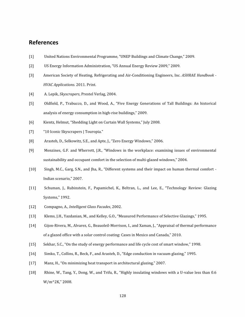
128
References
[1] United Nations Environmental Programme, “UNEP Buildings and Climate Change,” 2009.
[2] US Energy Information Administration, “US Annual Energy Review 2009,” 2009.
[3] American Society of Heating, Refrigerating and Air-Conditioning Engineers, Inc. ASHRAE Handbook -
HVAC Applications. 2011. Print.
[4] A. Lepik, Skyscrapers, Prestel Verlag, 2004.
[5] Oldfield, P., Trabucco, D., and Wood, A., “Five Energy Generations of Tall Buildings: An historical
analysis of energy consumption in high-rise buildings,” 2009.
[6] Kientz, Helmut, “Shedding Light on Curtain Wall Systems,” July 2008.
[7] “10 Iconic Skyscrapers | Touropia.”
[8] Arasteh, D., Selkowitz, S.E., and Apte, J., “Zero Energy Windows,” 2006.
[9] Menzines, G.F. and Wherrett, J.R., “Windows in the workplace: examining issues of environmental
sustainability and occupant comfort in the selection of multi-glazed windows,” 2004.
[10] Singh, M.C., Garg, S.N., and Jha, R., “Different systems and their impact on human thermal comfort -
Indian scenario,” 2007.
[11] Schuman, J., Rubinstein, F., Papamichel, K., Beltran, L., and Lee, E., “Technology Review: Glazing
Systems,” 1992.
[12] Compagno, A., Intelligent Glass Facades, 2002.
[13] Klems, J.H., Yazdanian, M., and Kelley, G.O., “Measured Performance of Selective Glazings,” 1995.
[14] Gijon-Rivera, M., Alvarez, G., Beauoleil-Morrison, I., and Xaman, J., “Appraisal of thermal performance
of a glazed office with a solar control coating: Cases in Mexico and Canada,” 2010.
[15] Sekhar, S.C., “On the study of energy performance and life cycle cost of smart window,” 1998.
[16] Simko, T., Collins, R., Beck, F., and Arasteh, D., “Edge conduction in vacuum glazing,” 1995.
[17] Manz, H., “On minimizing heat transport in architectural glazing,” 2007.
[18] Rhine, W., Tang, Y., Dong, W., and Trifu, R., “Highly insulating windows with a U-value less than 0.6
W/m^2K,” 2008.
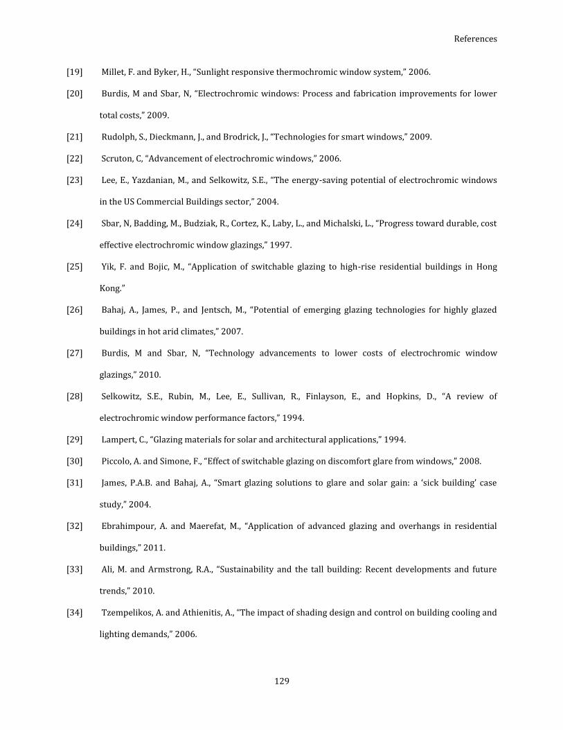
References
129
[19] Millet, F. and Byker, H., “Sunlight responsive thermochromic window system,” 2006.
[20] Burdis, M and Sbar, N, “Electrochromic windows: Process and fabrication improvements for lower
total costs,” 2009.
[21] Rudolph, S., Dieckmann, J., and Brodrick, J., “Technologies for smart windows,” 2009.
[22] Scruton, C, “Advancement of electrochromic windows,” 2006.
[23] Lee, E., Yazdanian, M., and Selkowitz, S.E., “The energy-saving potential of electrochromic windows
in the US Commercial Buildings sector,” 2004.
[24] Sbar, N, Badding, M., Budziak, R., Cortez, K., Laby, L., and Michalski, L., “Progress toward durable, cost
effective electrochromic window glazings,” 1997.
[25] Yik, F. and Bojic, M., “Application of switchable glazing to high-rise residential buildings in Hong
Kong.”
[26] Bahaj, A., James, P., and Jentsch, M., “Potential of emerging glazing technologies for highly glazed
buildings in hot arid climates,” 2007.
[27] Burdis, M and Sbar, N, “Technology advancements to lower costs of electrochromic window
glazings,” 2010.
[28] Selkowitz, S.E., Rubin, M., Lee, E., Sullivan, R., Finlayson, E., and Hopkins, D., “A review of
electrochromic window performance factors,” 1994.
[29] Lampert, C., “Glazing materials for solar and architectural applications,” 1994.
[30] Piccolo, A. and Simone, F., “Effect of switchable glazing on discomfort glare from windows,” 2008.
[31] James, P.A.B. and Bahaj, A., “Smart glazing solutions to glare and solar gain: a ‘sick building’ case
study,” 2004.
[32] Ebrahimpour, A. and Maerefat, M., “Application of advanced glazing and overhangs in residential
buildings,” 2011.
[33] Ali, M. and Armstrong, R.A., “Sustainability and the tall building: Recent developments and future
trends,” 2010.
[34] Tzempelikos, A. and Athienitis, A., “The impact of shading design and control on building cooling and
lighting demands,” 2006.
References
130
[35] Lee, E., DiBartolomeo, D.L., Vine, E.L., and Selkowitz, S.E., “Integrated performance of an automated
venetian blind/electric lighting system in a full-scale private office,” 1998.
[36] Sinclair, R., Phillips, D., and Mezhibovski, V., “Ventilating Facades,” 2009.
[37] Lee, E., “High performance commercial building facades,” 2002.
[38] Selkowitz, S.E., Aschenhoug, O., and Lee, E., “Advanced interactive facades - critical elements for
future green buildings?,” 2003.
[39] Guardo, A., Coussirat, M., Egusquiza, E., Alavedra, P., and Castilla, R., “A CFD approach to evaluate the
influence of construction and operation parameters on the performance of ATF in Mediterranean
climates,” 2009.
[40] [50] [38] Yeang, K., The Green Skyscraper, Prestel Verlag, 1999.
[41] Corgnati, S., Perino, M., and Serra, V., “Experimental assessment of the performance of an active
transparent facade during actual operating conditions,” 2007.
[42] Hamza, N., “Double versus single skin facades in hot arid climates,” 2004.
[43] Altan, H., Ward, I., Moheinikova, J., and Vajkay, F., “An internal assessment of the thermal comfort and
daylighting conditions of naturally ventilated building with an active glazed facade in a temperate
climate,” 2008.
[44] Cetiner, I. and Ozkan, E., “An approach for the evaluation of energy and cost efficiency of glass
facades,” 2004.
[45] Song, S.Y., Yi, J.S., and Koo, B.K., “Insulation plan of aluminum curtain wall-fastening unit for high-rise
residential complex,” 2007.
[46] Gustavsen, A., Jelle, B., Arasteh, D., and Kohler, C., “State-of-the-art highly insulating window frames -
research and market review,” 2007.
[47] Griffith, B., Finlayson, E., Yazdanian, M., and Arasteh, D., “The significance of bolts in the thermal
performance of curtain-wall frames for glazed facades,” 1997.
[48] Hwang, R.L. and Shu, S.Y., “Building envelope regulations on thermal comfort in glass facade
buildings and energy saving potential for PMV-based control,” 2010.
[49] Ge, H. and Fazio, P., “Experimental investigation of cold draft induced by two different types of
glazing panels in metal curtain walls,” 2003.

References
131
[50] Heiselberg, P., “Draught risk from cold vertical surfaces,” 1994.
[51] Heiselberg, P. and Bjorn, E., “Measures to avoid downdraft from large glazed facades,” 1995.
[52] Larsson, U. and Moshfegh, “Experimental investigation of downdraught from well-insulated
windows,” 2002.
[53] Tzempelikos, A. and Bessoudo, M., “Indoor thermal environmental conditions near glazed facades
with shading devices - Part II,” 2010.
[54] Goncalves, J. and Bode, K., “THe importance of real life data to support environmental claims for tall
buildings,” 2011.
[55] International Building Code, “Code and Commentary, Volume 1,” 2009.
[56] Lee, E., Selkowitz, S.E., Levi, M., Blanc, S., McConahey, E., McClintock, M., and Hakkarainen, P., “Active
load management with advaced window wall systems: research and industry perspectives,” 2002.
[57] Etheridge, DW and Ford, B., “Natural Ventilation of Tall Buildings,” 2008.
[58] Ali, M. and Armstrong, R.A., “Overview of sustainable design factors in high-rise buildings,” 2008.
[59] Tzempelikos, A., Athienitis, A., and Karava, P., “Simulation of facade and envelope design options for
a new institutional building,” 2007.
[60] Li, D. and Tsang, E., “Energy performance of windows in high-rise residential buildings in Hong
Kong,” 2001.
[61] Lam, J., Wan, K., Tsang, C., and Yang, L., “Building energy efficiency in different climates,” 2008.
[62] Lam, J., Tsang, C., Li, D., and Cheung, S., “Residential building envelope heat gain and cooling energy
requirements.”
[63] Li, D. and Tsang, E., “An analysis of daylighting performance for office buildings in Hong Kong,” 2007.
[64] Niu, J., “Some significant environmental issues in high-rise residential building design in urban
areas.”
[65] Wan, K. and Yik, F., “Building design and energy end-use characteristics of high-rise residential
buildings in Hong-Kong,” 2003.
[66] Wong, S.L., Wan, K., Li, D., and Lam, J., “Impact of climate change on residential building envelope
cooling loads in subtropical climates,” 2010.

References
132
[67] Bojic, M. and Yik, F., “Application of advanced glazing to high-rise residential buildings in Hong
Kong,” 2007.
[68] Cheung, C., Fuller, R., and Luther, M., “Energy-efficient envelope design for high-rise apartments,”
2004.
[69] Zheng, G., Jing, Y., Huang, H., and Gao, Y., “Application of improved grey relational projection method
to evaluate sustainable building envelope performance,” 2009.
[70] Yoshino, H., Yoshino, Y., Zhang, Q., Mochida, A., LI, N., and Li, Z., “Indoor thermal environment and
energy saving for urban residential buildings in China,” 2006.
[71] Tzempelikos, A., Athienitis, A., and Nazos, A., “Integrated design of perimeter zones with glass
facades,” 2010.
[72] Lee, E., Selkowitz, S.E., Rubinstein, F., Klems, J.H., Beltran, L., and DiBartolomeo, D.L., “A
comprehensive approach to integrated envelope and lighting systems for new commercial buildings,”
1994.
[73] Armstrong, P., Dirks, J., Reilly, R., Currie, B., Nesse, R., Komarov, O., and Necrasov, B., “Russian
apartment building thermal response models for retrofit selection and verification,” 1999.
[74] Tang, D. and Kim, J., “Simulation support for sustainable design of buildings,” 2004.
[75] Assem, E.O. and Al-Mumin, A.A., “Code compliance of fully glazed tall office buildings in hot climate,”
2010.
[76] Dalton, K. and John, R., “Towards more sustainable tall buildings,” 2008.
[77] “Empire State Building White Paper,” 2010.
[78] Fluhrer, C., Maurer, E., and Deshmukh, A., “Achieving radically energy efficient retrofits: The Empire
State Building Example,” 2010.
[79] “Transforming an Icon.”
[80] Spirito, G. and Terranova, A., New Urban Giants, White Star S.p.A., 2008.
[81] “Philadelphia Announces the Tallest LEED Certified Building in US | Inhabitat - Green Design Will
Save the World.”
[82] “Robert A.M. Stern Architects - Comcast Center.”
[83] Genge, C., “Controlling Air Leakage In Tall Buildings.” 2009. ASHRAE Journal.

References
133
[84] Deru, M., Field, K., Studer, D., Benne, K., Griffith, B., Torcellini, P., Liu, B., Halverson, M., Winiarski, D.,
Rosenberg, M., Yazdanian, M., Huang, J., Crawley, D., “U.S. Department of Energy Commercial
Reference Building Models of the National Building Stock,” Feb. 2011.
[85] “EnergyPlus Energy Simulation Software,” http://apps1.eere.energy.gov/buildings/energyplus, Dec.
7, 2011.
[86] The Skyscraper Center, The Global Tall Building Database of the Council on Tall Buildings and Urban
Habitat:, http://www.ctbuh.org/TallBuildings/HeightStatistics/Criteria/tabid/446/language/en-
US/Default.aspx . 2012.
[87] Energy Standard for Buildings Except Low-Rise Residential Buildings, ANSI/ASHRAE/IESNA
Standard 90.1-2004. 2004.
[88] Energy Standard for Buildings Except Low-Rise Residential Buildings, ANSI/ASHRAE/IESNA
Standard 90.1-2010. 2010.
[89] BuildingGreen.com, buildinggreen.com, April. 2012.
[90] Serious Windows, http://www.seriouswindows.com/, April. 2012.
[91] Leach, M., Lobato, C., Hirsch, A., Pless, S., Torcellini, P. “Technical Support Document: Strategies for
50% Energy Savings in Large Office Buildings.” September 2010. National Renewable Energy
Laboratory.
[92] Winiarski, D., Shankle, S., Hail, J., Liu, B. “Appendix B: Energy and Construction Cost Estimates.”
[93] Viracon, Inc. http://www.viracon.com/ April 2012.
[94] Trane Quick Reference for Efficient Chiller System Design.
http://www.trane.com/commercial/uploads/pdf/865/ctv-trt-001-en.pdf. April 2012.
[95] Tredinnick, S. “Benefits of Economic Analyses (part 2): Real-world examples.” 2010. International
District Energy Association.
[96] “ASHRAE NOPR TSD Chapter 5: Life Cycle Cost and Payback Period Analysis.”
https://www1.eere.energy.gov/buildings/appliance_standards/commercial/pdfs/ch_5_ashrae_nopr
_tsd.pdf. April 2012.
[97] Gibson, Todd Allen. “Daylighting Software Validation Study and Development of a Simplified Method
to Predict the Energy Impacts of Façade Design and Daylighting Control in Private Offices.” 2003.

134
Appendix A: Envelope Values
Roof U-values (Btu/h*ft
2*°F) for New Construction by Location
Location DOE Benchmark
(ASHRAE 90.1-1994)
Highrise Baseline
(ASHRAE 90.1-2010)
Miami, FL (1A) 0.063 0.063
Houston, TX (2A) 0.063 0.048
Phoenix, AZ (2B) 0.063 0.048
Atlanta, GA (3A) 0.063 0.048
San Francisco, CA (3C) 0.063 0.048
Baltimore, MD (4A) 0.063 0.048
Seattle, WA (4C) 0.063 0.048
Chicago, IL (5A) 0.063 0.048
Denver, CO (5B) 0.063 0.048
Helena, MT (6B) 0.063 0.048
Duluth, MN (7) 0.063 0.048
Wall U-values (Btu/h*ft2*°F) for New Construction by Location
Location DOE Benchmark
(ASHRAE 90.1-1994)
Highrise Baseline
(ASHRAE 90.1-2010) Steel Frame Mass Steel Frame Mass
Miami, FL (1A) 0.124 0.580 0.124 0.580
Houston, TX (2A) 0.124 0.580 0.124 0.151
Phoenix, AZ (2B) 0.124 0.580 0.124 0.151
Atlanta, GA (3A) 0.124 0.151 0.084 0.123
San Francisco, CA (3C) 0.124 0.580 0.084 0.123
Baltimore, MD (4A) 0.124 0.580 0.064 0.104
Seattle, WA (4C) 0.124 0.151 0.064 0.104
Chicago, IL (5A) 0.084 0.151 0.064 0.090
Denver, CO (5B) 0.084 0.151 0.064 0.090
Helena, MT (6B) 0.084 0.123 0.064 0.080
Duluth, MN (7) 0.084 0.123 0.064 0.071

Appendix A: Envelope Values
135
Wall Below-Grade C-factor (Btu/h*ft2*°F) for New Construction by Location
Location DOE Benchmark
(ASHRAE 90.1-1994) Highrise Baseline
(ASHRAE 90.1-2010)
C-factor Ins. Req’d C-factor Ins. Req’d
Miami, FL (1A) 1.140 NR 1.140 NR
Houston, TX (2A) 1.140 NR 1.140 NR
Phoenix, AZ (2B) 1.140 NR 1.140 NR
Atlanta, GA (3A) 1.140 NR 1.140 NR
San Francisco, CA (3C) 1.140 NR 1.140 NR
Baltimore, MD (4A) 1.140 NR 1.140 NR
Seattle, WA (4C) 1.140 NR 1.140 NR
Chicago, IL (5A) 1.140 NR 0.119 R-7.5 ci
Denver, CO (5B) 1.140 NR 0.119 R-7.5 ci
Helena, MT (6B) 1.140 NR 0.119 R-7.5 ci
Duluth, MN (7) 0.119 R-7.5 ci 0.119 R-7.5 ci
Slab-on-grade Floors F-factor (Btu/h*ft*°F) for New Construction by Location
Location DOE Benchmark
(ASHRAE 90.1-1994)
Highrise Baseline
(ASHRAE 90.1-2010)
F-factor Ins. Req’d F-factor Ins. Req’d
Miami, FL (1A) 0.73 NR 0.73 NR Houston, TX (2A) 0.73 NR 0.73 NR Phoenix, AZ (2B) 0.73 NR 0.73 NR Atlanta, GA (3A) 0.73 NR 0.73 NR
San Francisco, CA (3C) 0.73 NR 0.73 NR Baltimore, MD (4A) 0.73 NR 0.73 NR
Seattle, WA (4C) 0.73 NR 0.73 NR Chicago, IL (5A) 0.73 NR 0.73 NR
Denver, CO (5B) 0.73 NR 0.73 NR Helena, MT (6B) 0.73 NR 0.54 R-10 for 24 in
Duluth, MN (7) 0.73 NR 0.52 R-15 for 24 in

Appendix A: Envelope Values
136
Window Overall U-value (Btu/h*ft2*°F) and SHGC for New Construction by Location
Location DOE Benchmark
(ASHRAE 90.1-1994)
Highrise Baseline
(ASHRAE 90.1-2010)
U-value SHGC U-value SHGC
Miami, FL (1A) 1.22 0.25 1.20 0.25 Houston, TX (2A) 1.22 0.25 0.70 0.25 Phoenix, AZ (2B) 1.22 0.25 0.70 0.25 Atlanta, GA (3A) 0.57 0.25 0.60 0.25
San Francisco, CA (3C) 1.22 0.34 0.60 0.25 Baltimore, MD (4A) 0.57 0.39 0.50 0.40
Seattle, WA (4C) 0.57 0.39 0.50 0.40 Chicago, IL (5A) 0.57 0.39 0.45 0.40
Denver, CO (5B) 0.57 0.39 0.45 0.40 Helena, MT (6B) 0.57 0.39 0.45 0.40
Duluth, MN (7) 0.57 0.49 0.40 0.45

137
Appendix B: Window-to-Wall Ratio Results
Miami, FL WTW Ratio Results
-40.00%
-20.00%
0.00%
20.00%
40.00%
60.00%
80.00%
100.00%
120.00%
140.00%
50% WTWRatio
60% WTWRatio
70% WTWRatio
80% WTWRatio
90% WTWRatio
95% WTWRatio
Sn
esi
ble
Ga
ins
% D
iff
fro
m
Ba
seli
ne
Occupants (+)
Lights (+)
Equipment (+)
Window (+)
Infiltration )+)
Opaque and other (+)
Window (-)
Infiltration (-)
-50.00%
0.00%
50.00%
100.00%
150.00%
200.00%
250.00%
300.00%
350.00%
400.00%
450.00%
40% 50% 60% 70% 80% 90% 100%
% D
iffe
ren
ce f
rom
Ba
seli
ne
WTW Ratio
Cooling
Heating
-10000
0
10000
20000
30000
40000
50000
60000
40% WTWRatio
50% WTWRatio
60% WTWRatio
70% WTWRatio
80% WTWRatio
90% WTWRatio
95% WTWRatio
Se
nsi
ble
Ga
ins
(GJ_
Opaque and other (-)
Infiltration (-)
Window (-)
Opaque and other (+)
Infiltration )+)
Window (+)
Equipment (+)
Figure 80: WTW Ratio - Sensible Gains - Miami, FL
Figure 81: WTW Ratio - Sensible Gains Change from Baseline - Miami, FL
Figure 82: WTW Ratio - Heating and Cooling Energy % Difference from Baseline - Miami, FL

Appendix B: Window-to-Wall Ratio Results
138
Houston, TX Results
-10000
0
10000
20000
30000
40000
50000
40% WTWRatio
50% WTWRatio
60% WTWRatio
70% WTWRatio
80% WTWRatio
90% WTWRatio
95% WTWRatio
Opaque and other (-)
Infiltration (-)
Window (-)
Opaque and other (+)
Infiltration )+)
Window (+)
Equipment (+)
Lights (+)
Occupants (+)
-20.00%
0.00%
20.00%
40.00%
60.00%
80.00%
100.00%
120.00%
140.00%
160.00%
50% WTWRatio
60% WTWRatio
70% WTWRatio
80% WTWRatio
90% WTWRatio
95% WTWRatio
Occupants (+)
Lights (+)
Equipment (+)
Window (+)
Infiltration )+)
Opaque and other (+)
Window (-)
Infiltration (-)
Opaque and other (-)
-500.00
0.00
500.00
1000.00
1500.00
2000.00
2500.00
3000.00
3500.00
4000.00
50% WTW Ratio 60% WTW Ratio 70% WTW Ratio 80% WTW Ratio 90% WTW Ratio 95% WTW Ratio
Dif
fere
nce
fro
m B
ase
lin
e (
GJ_
HeatRejection
Pumps
Fans
Cooling
Heating
Figure 83: WTW Ratio - Energy Consumption Difference from Baseline - Miami, FL
Figure 84: WTW Ratio - Sensible Gains - Houston, TX
Figure 85: WTW Ratio - Sensible Gains Change from Baseline - Houston, TX

Appendix B: Window-to-Wall Ratio Results
139
Phoenix, AZ WTW Ratio Results
-50.00%
0.00%
50.00%
100.00%
150.00%
200.00%
250.00%
40% 50% 60% 70% 80% 90% 100%
Cooling
Heating
-3000.00
-2000.00
-1000.00
0.00
1000.00
2000.00
3000.00
4000.00
5000.00
50% WTWRatio
60% WTWRatio
70% WTWRatio
80% WTWRatio
90% WTWRatio
95% WTWRatio
Heat Rejection
Pumps
Fans
Cooling
Heating
-10000
0
10000
20000
30000
40000
50000
60000
40% WTWRatio
50% WTWRatio
60% WTWRatio
70% WTWRatio
80% WTWRatio
90% WTWRatio
95% WTWRatio
Opaque and other (-)
Infiltration (-)
Window (-)
Opaque and other (+)
Infiltration )+)
Window (+)
Equipment (+)
Lights (+)
Occupants (+)
Figure 88: WTW Ratio - Sensible Gains - Phoenix, AZ
Figure 87: WTW Ratio - Heating and Cooling Energy % Difference from Baseline -
Figure 86: WTW Ratio - Energy Consumption Difference from Baseline - Houston, TX

Appendix B: Window-to-Wall Ratio Results
140
0.00%
50.00%
100.00%
150.00%
200.00%
250.00%
40% 50% 60% 70% 80% 90% 100%
Cooling
Heating
-20.00%
0.00%
20.00%
40.00%
60.00%
80.00%
100.00%
120.00%
140.00%
50% WTWRatio
60% WTWRatio
70% WTWRatio
80% WTWRatio
90% WTWRatio
95% WTWRatio
Occupants (+)
Lights (+)
Equipment (+)
Window (+)
Infiltration )+)
Opaque and other (+)
Window (-)
0.00
1000.00
2000.00
3000.00
4000.00
5000.00
6000.00
50% WTW Ratio60% WTW Ratio70% WTW Ratio80% WTW Ratio90% WTW Ratio95% WTW Ratio
Heat Rejection
Pumps
Fans
Cooling
Heating
Figure 89: WTW Ratio - Sensible Gains Change from Baseline - Phoenix, AZ
Figure 91: WTW Ratio - Heating and Cooling Energy % Difference from Baseline - Phoenix, AZ
Figure 90: WTW Ratio - Energy Consumption Difference from Baseline - Phoenix, AZ
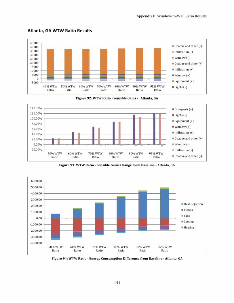
Appendix B: Window-to-Wall Ratio Results
141
Atlanta, GA WTW Ratio Results
-5000
0
5000
10000
15000
20000
25000
30000
35000
40000
45000
40% WTWRatio
50% WTWRatio
60% WTWRatio
70% WTWRatio
80% WTWRatio
90% WTWRatio
95% WTWRatio
Opaque and other (-)
Infiltration (-)
Window (-)
Opaque and other (+)
Infiltration )+)
Window (+)
Equipment (+)
Lights (+)
-20.00%
0.00%
20.00%
40.00%
60.00%
80.00%
100.00%
120.00%
140.00%
50% WTWRatio
60% WTWRatio
70% WTWRatio
80% WTWRatio
90% WTWRatio
95% WTWRatio
Occupants (+)
Lights (+)
Equipment (+)
Window (+)
Infiltration )+)
Opaque and other (+)
Window (-)
Infiltration (-)
Opaque and other (-)
-4000.00
-3000.00
-2000.00
-1000.00
0.00
1000.00
2000.00
3000.00
4000.00
5000.00
6000.00
50% WTWRatio
60% WTWRatio
70% WTWRatio
80% WTWRatio
90% WTWRatio
95% WTWRatio
Heat Rejection
Pumps
Fans
Cooling
Heating
Figure 92: WTW Ratio - Sensible Gains - Atlanta, GA
Figure 93: WTW Ratio - Sensible Gains Change from Baseline - Atlanta, GA
Figure 94: WTW Ratio - Energy Consumption Difference from Baseline - Atlanta, GA

Appendix B: Window-to-Wall Ratio Results
142
San Francisco, CA WTW Ratio Results
-40.00%
-20.00%
0.00%
20.00%
40.00%
60.00%
80.00%
100.00%
120.00%
140.00%
160.00%
180.00%
40% 50% 60% 70% 80% 90% 100%
Cooling
Heating
-10000
-5000
0
5000
10000
15000
20000
25000
30000
35000
40000
40% WTWRatio
50% WTWRatio
60% WTWRatio
70% WTWRatio
80% WTWRatio
90% WTWRatio
95% WTWRatio
Opaque and other (-)
Infiltration (-)
Window (-)
Opaque and other (+)
Infiltration )+)
Window (+)
Equipment (+)
Lights (+)
Occupants (+)
-20.00%
0.00%
20.00%
40.00%
60.00%
80.00%
100.00%
120.00%
140.00%
50% WTWRatio
60% WTWRatio
70% WTWRatio
80% WTWRatio
90% WTWRatio
95% WTWRatio
Occupants (+)
Lights (+)
Equipment (+)
Window (+)
Infiltration )+)
Opaque and other (+)
Window (-)
Infiltration (-)
Opaque and other (-)
Figure 96: WTW Ratio - Sensible Gains - San Francisco, CA
Figure 97: WTW Ratio - Sensible Gains Change from Baseline - San Francisco, CA
Figure 95: WTW Ratio - Heating and Cooling Energy % Difference from Baseline - Atlanta, GA

Appendix B: Window-to-Wall Ratio Results
143
Baltimore, MD WTW Ratio Results
0.00%
50.00%
100.00%
150.00%
200.00%
250.00%
300.00%
40% 50% 60% 70% 80% 90% 100%
Cooling
Heating
-10000
-5000
0
5000
10000
15000
20000
25000
30000
35000
40000
45000
40% WTWRatio
50% WTWRatio
60% WTWRatio
70% WTWRatio
80% WTWRatio
90% WTWRatio
95% WTWRatio
Opaque and other (-)
Infiltration (-)
Window (-)
Opaque and other (+)
Infiltration )+)
Window (+)
Equipment (+)
Lights (+)
Occupants (+)
0.00
1000.00
2000.00
3000.00
4000.00
5000.00
6000.00
50% WTWRatio
60% WTWRatio
70% WTWRatio
80% WTWRatio
90% WTWRatio
95% WTWRatio
Heat Rejection
Pumps
Fans
Cooling
Heating
Figure 100: WTW Ratio - Sensible Gains - Baltimore, MD
Figure 99: WTW Ratio - Heating and Cooling Energy % Difference from Baseline - San Francisco, CA
Figure 98: WTW Ratio - Energy Consumption Difference from Baseline - San Francisco, CA

Appendix B: Window-to-Wall Ratio Results
144
-20.00%
0.00%
20.00%
40.00%
60.00%
80.00%
100.00%
120.00%
140.00%
50% WTWRatio
60% WTWRatio
70% WTWRatio
80% WTWRatio
90% WTWRatio
95% WTWRatio
Occupants (+)
Lights (+)
Equipment (+)
Window (+)
Infiltration )+)
Opaque and other (+)
Window (-)
Infiltration (-)
Opaque and other (-)
-40.00%
-20.00%
0.00%
20.00%
40.00%
60.00%
80.00%
100.00%
120.00%
40% 50% 60% 70% 80% 90% 100%
Cooling
Heating
-6000.00
-4000.00
-2000.00
0.00
2000.00
4000.00
6000.00
8000.00
50% WTWRatio
60% WTWRatio
70% WTWRatio
80% WTWRatio
90% WTWRatio
95% WTWRatio
Heat Rejection
Pumps
Fans
Cooling
Heating
Figure 101: WTW Ratio - Sensible Gains Change from Baseline - Baltimore, MD
Figure 103: WTW Ratio - Heating and Cooling Energy % Difference from Baseline - Baltimore, MD
Figure 102: WTW Ratio - Energy Consumption Difference from Baseline - Baltimore, MD
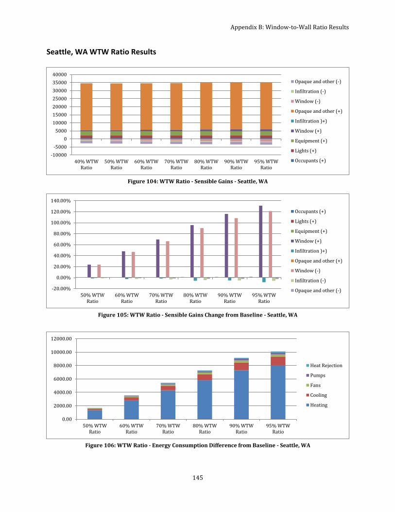
Appendix B: Window-to-Wall Ratio Results
145
Seattle, WA WTW Ratio Results
-10000
-5000
0
5000
10000
15000
20000
25000
30000
35000
40000
40% WTWRatio
50% WTWRatio
60% WTWRatio
70% WTWRatio
80% WTWRatio
90% WTWRatio
95% WTWRatio
Opaque and other (-)
Infiltration (-)
Window (-)
Opaque and other (+)
Infiltration )+)
Window (+)
Equipment (+)
Lights (+)
Occupants (+)
-20.00%
0.00%
20.00%
40.00%
60.00%
80.00%
100.00%
120.00%
140.00%
50% WTWRatio
60% WTWRatio
70% WTWRatio
80% WTWRatio
90% WTWRatio
95% WTWRatio
Occupants (+)
Lights (+)
Equipment (+)
Window (+)
Infiltration )+)
Opaque and other (+)
Window (-)
Infiltration (-)
Opaque and other (-)
0.00
2000.00
4000.00
6000.00
8000.00
10000.00
12000.00
50% WTWRatio
60% WTWRatio
70% WTWRatio
80% WTWRatio
90% WTWRatio
95% WTWRatio
Heat Rejection
Pumps
Fans
Cooling
Heating
Figure 104: WTW Ratio - Sensible Gains - Seattle, WA
Figure 105: WTW Ratio - Sensible Gains Change from Baseline - Seattle, WA
Figure 106: WTW Ratio - Energy Consumption Difference from Baseline - Seattle, WA

Appendix B: Window-to-Wall Ratio Results
146
Chicago, IL WTW Ratio Results
0.00%
20.00%
40.00%
60.00%
80.00%
100.00%
120.00%
140.00%
160.00%
180.00%
40% 50% 60% 70% 80% 90% 100%
Cooling
Heating
-10000
-5000
0
5000
10000
15000
20000
25000
30000
35000
40000
40% WTWRatio
50% WTWRatio
60% WTWRatio
70% WTWRatio
80% WTWRatio
90% WTWRatio
95% WTWRatio
Opaque and other (-)
Infiltration (-)
Window (-)
Opaque and other (+)
Infiltration )+)
Window (+)
Equipment (+)
Lights (+)
Occupants (+)
-20.00%
0.00%
20.00%
40.00%
60.00%
80.00%
100.00%
120.00%
140.00%
50% WTWRatio
60% WTWRatio
70% WTWRatio
80% WTWRatio
90% WTWRatio
95% WTWRatio
Occupants (+)
Lights (+)
Equipment (+)
Window (+)
Infiltration )+)
Opaque and other (+)
Window (-)
Infiltration (-)
Opaque and other (-)
Figure 108: WTW Ratio - Sensible Gains - Chicago, IL
Figure 109: WTW Ratio - Sensible Gains Change from Baseline - Chicago, IL
Figure 107: WTW Ratio - Heating and Cooling Energy % Difference from Baseline - Seattle, WA

Appendix B: Window-to-Wall Ratio Results
147
Denver, CO WTW Ratio Results
0.00
2000.00
4000.00
6000.00
8000.00
10000.00
12000.00
50% WTWRatio
60% WTWRatio
70% WTWRatio
80% WTWRatio
90% WTWRatio
95% WTWRatio
Heat Rejection
Pumps
Fans
Cooling
Heating
0.00%
10.00%
20.00%
30.00%
40.00%
50.00%
60.00%
70.00%
80.00%
90.00%
40% 50% 60% 70% 80% 90% 100%
Cooling
Heating
-10000
-5000
0
5000
10000
15000
20000
25000
30000
35000
40000
45000
40% WTWRatio
50% WTWRatio
60% WTWRatio
70% WTWRatio
80% WTWRatio
90% WTWRatio
95% WTWRatio
Opaque and other (-)
Infiltration (-)
Window (-)
Opaque and other (+)
Infiltration )+)
Window (+)
Equipment (+)
Lights (+)
Occupants (+)
Figure 112: WTW Ratio - Sensible Gains - Denver, CO
Figure 111: WTW Ratio - Heating and Cooling Energy % Difference from Baseline - Chicago, IL
Figure 110: WTW Ratio - Energy Consumption Difference from Baseline - Chicago, IL

Appendix B: Window-to-Wall Ratio Results
148
-20.00%
0.00%
20.00%
40.00%
60.00%
80.00%
100.00%
120.00%
140.00%
50% WTWRatio
60% WTWRatio
70% WTWRatio
80% WTWRatio
90% WTWRatio
95% WTWRatio
Occupants (+)
Lights (+)
Equipment (+)
Window (+)
Infiltration )+)
Opaque and other (+)
Window (-)
Infiltration (-)
0.00
1000.00
2000.00
3000.00
4000.00
5000.00
6000.00
7000.00
8000.00
9000.00
50% WTWRatio
60% WTWRatio
70% WTWRatio
80% WTWRatio
90% WTWRatio
95% WTWRatio
Heat Rejection
Pumps
Fans
Cooling
Heating
0.00%
20.00%
40.00%
60.00%
80.00%
100.00%
120.00%
140.00%
40% 50% 60% 70% 80% 90% 100%
Cooling
Heating
Figure 113: WTW Ratio - Sensible Gains Change from Baseline - Denver, CO
Figure 115: WTW Ratio - Heating and Cooling Energy % Difference from Baseline - Denver, CO
Figure 114: WTW Ratio - Energy Consumption Difference from Baseline - Denver, CO

Appendix B: Window-to-Wall Ratio Results
149
Helena, MT WTW Ratio Results
-10000
-5000
0
5000
10000
15000
20000
25000
30000
35000
40000
40% WTWRatio
50% WTWRatio
60% WTWRatio
70% WTWRatio
80% WTWRatio
90% WTWRatio
95% WTWRatio
Opaque and other (-)
Infiltration (-)
Window (-)
Opaque and other (+)
Infiltration )+)
Window (+)
Equipment (+)
Lights (+)
Occupants (+)
-20.00%
0.00%
20.00%
40.00%
60.00%
80.00%
100.00%
120.00%
140.00%
50% WTWRatio
60% WTWRatio
70% WTWRatio
80% WTWRatio
90% WTWRatio
95% WTWRatio
Occupants (+)
Lights (+)
Equipment (+)
Window (+)
Infiltration )+)
Opaque and other (+)
Window (-)
Infiltration (-)
Opaque and other (-)
0.00
2000.00
4000.00
6000.00
8000.00
10000.00
12000.00
50% WTWRatio
60% WTWRatio
70% WTWRatio
80% WTWRatio
90% WTWRatio
95% WTWRatio
Heat Rejection
Pumps
Fans
Cooling
Heating
Figure 116: WTW Ratio - Sensible Gains - Helena, MT
Figure 117: WTW Ratio - Sensible Gains Change from Baseline - Helena, MT
Figure 118: WTW Ratio - Energy Consumption Difference from Baseline - Helena, MT
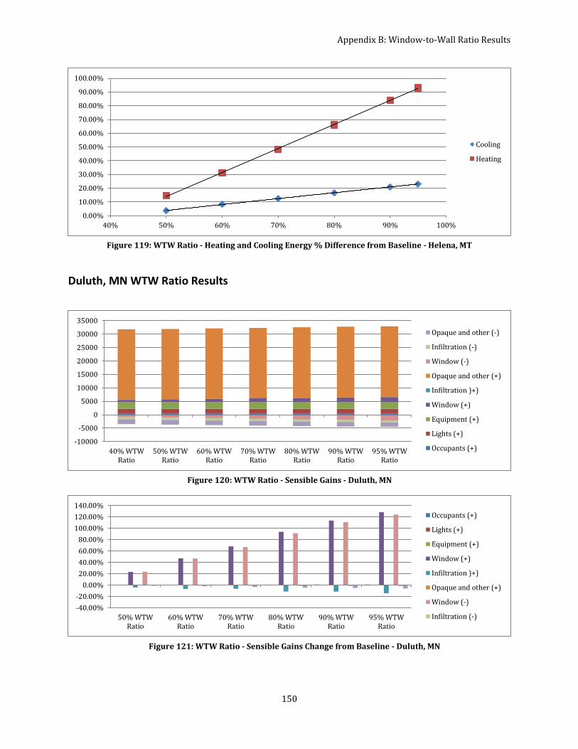
Appendix B: Window-to-Wall Ratio Results
150
Duluth, MN WTW Ratio Results
0.00%
10.00%
20.00%
30.00%
40.00%
50.00%
60.00%
70.00%
80.00%
90.00%
100.00%
40% 50% 60% 70% 80% 90% 100%
Cooling
Heating
-10000
-5000
0
5000
10000
15000
20000
25000
30000
35000
40% WTWRatio
50% WTWRatio
60% WTWRatio
70% WTWRatio
80% WTWRatio
90% WTWRatio
95% WTWRatio
Opaque and other (-)
Infiltration (-)
Window (-)
Opaque and other (+)
Infiltration )+)
Window (+)
Equipment (+)
Lights (+)
Occupants (+)
-40.00%
-20.00%
0.00%
20.00%
40.00%
60.00%
80.00%
100.00%
120.00%
140.00%
50% WTWRatio
60% WTWRatio
70% WTWRatio
80% WTWRatio
90% WTWRatio
95% WTWRatio
Occupants (+)
Lights (+)
Equipment (+)
Window (+)
Infiltration )+)
Opaque and other (+)
Window (-)
Infiltration (-)
Figure 120: WTW Ratio - Sensible Gains - Duluth, MN
Figure 121: WTW Ratio - Sensible Gains Change from Baseline - Duluth, MN
Figure 119: WTW Ratio - Heating and Cooling Energy % Difference from Baseline - Helena, MT

Appendix B: Window-to-Wall Ratio Results
151
0.00
2000.00
4000.00
6000.00
8000.00
10000.00
12000.00
14000.00
50% WTWRatio
60% WTWRatio
70% WTWRatio
80% WTWRatio
90% WTWRatio
95% WTWRatio
Heat Rejection
Pumps
Fans
Cooling
Heating
0.00%
10.00%
20.00%
30.00%
40.00%
50.00%
60.00%
70.00%
40% 50% 60% 70% 80% 90% 100%
Cooling
Heating
Figure 123: WTW Ratio - Heating and Cooling Energy % Difference from Baseline - Duluth, MN
Figure 122: WTW Ratio - Energy Consumption Difference from Baseline - Duluth, MN

152
Appendix C: Window U-values Results
Miami, FL Window U-value Results
Figure 124: Window U-value - Sensible Gains % Difference from Baseline - Miami, FL
Figure 125: Window U-value - Energy Consumption Difference from Baseline - Miami, FL
Figure 126: Window U-value - Heating and Cooling Energy % Difference from Baseline - Miami, FL
-100.00%
-80.00%
-60.00%
-40.00%
-20.00%
0.00%
20.00%
40.00%
40% WTW,U-0.92
40% WTW,U-0.64
40% WTW,U-0.36
40% WTW,U-0.08
70% WTW,U-0.92
70% WTW,U-0.64
70% WTW,U-0.36
70% WTW,U-0.08
Occupants (+)
Lights (+)
Equipment (+)
Window (+)
Infiltration )+)
Opaque and other (+)
Window (-)
Infiltration (-)
-1800.00
-1600.00
-1400.00
-1200.00
-1000.00
-800.00
-600.00
-400.00
-200.00
0.00
200.00
40% WTW,U-0.92
40% WTW,U-0.64
40% WTW,U-0.36
40% WTW,U-0.08
70% WTW,U-0.92
70% WTW,U-0.64
70% WTW,U-0.36
70% WTW,U-0.08
Heat Rejection
Pumps
Fans
Cooling
Heating
-120.00%
-100.00%
-80.00%
-60.00%
-40.00%
-20.00%
0.00%
0.00 0.10 0.20 0.30 0.40 0.50 0.60 0.70 0.80 0.90 1.00Cooling 40%WTW
Heating 40%WtW
Cooling 70%WTW
Heating 70%WTW

Appendix C: Window U-values Results
153
Houston, TX Window U-value Results
Figure 128: Window U-value - Sensible Gains % Difference from Baseline - Houston, TX
-100.00%
-80.00%
-60.00%
-40.00%
-20.00%
0.00%
20.00%
40.00%
40% WTW,U-0.545
40% WTW,U-0.39
40% WTW,U-0.235
40% WTW,U-0.08
70% WTW,U-0.545
70% WTW,U-0.39
70% WTW,U-0.235
70% WTW,U-0.08
Occupants (+)
Lights (+)
Equipment (+)
Window (+)
Infiltration )+)
Opaque and other (+)
Window (-)
Infiltration (-)
$(35,000.00)
$(30,000.00)
$(25,000.00)
$(20,000.00)
$(15,000.00)
$(10,000.00)
$(5,000.00)
$-
$5,000.00
$10,000.00
0.00 0.20 0.40 0.60 0.80 1.00 1.20 1.40
40% WTW Ratio
70% WTW Ratio
Figure 127: Window U-value Energy Cost Difference from Baseline - Miami, FL
-3500.00
-3000.00
-2500.00
-2000.00
-1500.00
-1000.00
-500.00
0.00
500.00
40% WTW,U-0.545
40% WTW,U-0.39
40% WTW,U-0.235
40% WTW,U-0.08
70% WTW,U-0.545
70% WTW,U-0.39
70% WTW,U-0.235
70% WTW,U-0.08
Heat Rejection
Pumps
Fans
Cooling
Heating
Figure 129: Window U-value Energy Consumption Difference from Baseline - Houston, TX

Appendix C: Window U-values Results
154
Phoenix, AZ Window U-value Results
Figure 132: Window U-value - Sensible Gains % Difference from Baseline - Phoenix, AZ
-100.00%
-80.00%
-60.00%
-40.00%
-20.00%
0.00%
20.00%
40.00%
40% WTW,U-0.545
40% WTW,U-0.39
40% WTW,U-0.235
40% WTW,U-0.08
70% WTW,U-0.545
70% WTW,U-0.39
70% WTW,U-0.235
70% WTW,U-0.08
Occupants (+)
Lights (+)
Equipment (+)
Window (+)
Infiltration )+)
Opaque and other (+)
Window (-)
Infiltration (-)
$(45,000.00)
$(40,000.00)
$(35,000.00)
$(30,000.00)
$(25,000.00)
$(20,000.00)
$(15,000.00)
$(10,000.00)
$(5,000.00)
$-
0.000 0.100 0.200 0.300 0.400 0.500 0.600 0.700 0.800
40% WTW Ratio
70% WTW Ratio
-100.00%
-90.00%
-80.00%
-70.00%
-60.00%
-50.00%
-40.00%
-30.00%
-20.00%
-10.00%
0.00%
0.000 0.100 0.200 0.300 0.400 0.500 0.600Cooling40% WTW
Heating40% WtW
Cooling70% WTW
Heating70% WTW
Figure 130: Window U-value - Heating and Cooling Energy % Difference from Baseline – Houston, TX
Figure 131: Window U-value - Energy Cost Difference from Baseline- Houston, TX
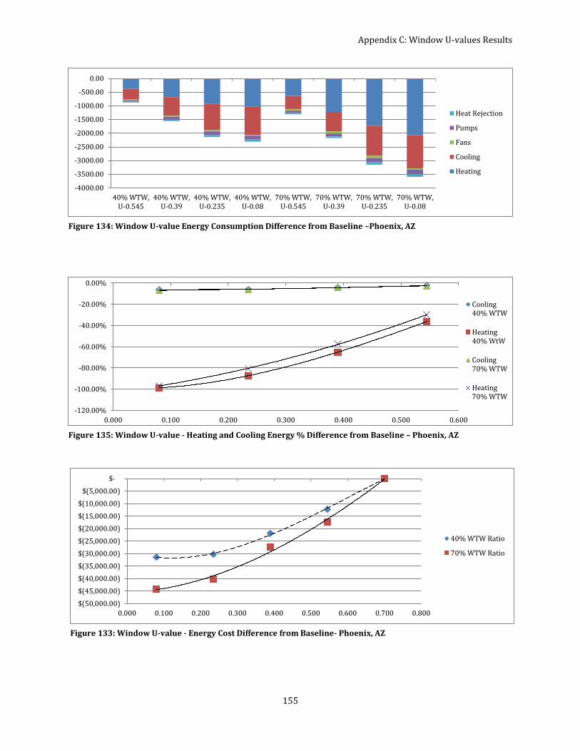
Appendix C: Window U-values Results
155
$(50,000.00)
$(45,000.00)
$(40,000.00)
$(35,000.00)
$(30,000.00)
$(25,000.00)
$(20,000.00)
$(15,000.00)
$(10,000.00)
$(5,000.00)
$-
0.000 0.100 0.200 0.300 0.400 0.500 0.600 0.700 0.800
40% WTW Ratio
70% WTW Ratio
-120.00%
-100.00%
-80.00%
-60.00%
-40.00%
-20.00%
0.00%
0.000 0.100 0.200 0.300 0.400 0.500 0.600
Cooling40% WTW
Heating40% WtW
Cooling70% WTW
Heating70% WTW
-4000.00
-3500.00
-3000.00
-2500.00
-2000.00
-1500.00
-1000.00
-500.00
0.00
40% WTW,U-0.545
40% WTW,U-0.39
40% WTW,U-0.235
40% WTW,U-0.08
70% WTW,U-0.545
70% WTW,U-0.39
70% WTW,U-0.235
70% WTW,U-0.08
Heat Rejection
Pumps
Fans
Cooling
Heating
Figure 134: Window U-value Energy Consumption Difference from Baseline –Phoenix, AZ
Figure 135: Window U-value - Heating and Cooling Energy % Difference from Baseline – Phoenix, AZ
Figure 133: Window U-value - Energy Cost Difference from Baseline- Phoenix, AZ

Appendix C: Window U-values Results
156
Atlanta, GA Window U-value Results
-100.00%
-80.00%
-60.00%
-40.00%
-20.00%
0.00%
20.00%
0.00 0.05 0.10 0.15 0.20 0.25 0.30 0.35 0.40 0.45 0.50
Cooling40% WTW
Heating40% WtW
Cooling70% WTW
Heating70% WTW
-6000.00
-5000.00
-4000.00
-3000.00
-2000.00
-1000.00
0.00
1000.00
2000.00
40% WTW,U-0.47
40% WTW,U-0.34
40% WTW,U-0.21
40% WTW,U-0.08
70% WTW,U-0.47
70% WTW,U-0.34
70% WTW,U-0.21
70% WTW,U-0.08
Heat Rejection
Pumps
Fans
Cooling
Heating
-100.00%
-80.00%
-60.00%
-40.00%
-20.00%
0.00%
20.00%
40.00%
40% WTW,U-0.47
40% WTW,U-0.34
40% WTW,U-0.21
40% WTW,U-0.08
70% WTW,U-0.47
70% WTW,U-0.34
70% WTW,U-0.21
70% WTW,U-0.08
Occupants (+)
Lights (+)
Equipment (+)
Window (+)
Infiltration )+)
Opaque and other (+)
Window (-)
Infiltration (-)
Opaque and other (-)
Figure 136: Window U-value - Sensible Gains % Difference from Baseline –Atlanta, GA
Figure 138: Window U-value Energy Consumption Difference from Baseline -Atlanta, GA
Figure 137: Window U-value - Heating and Cooling Energy % Difference from Baseline – Atlanta, GA

Appendix C: Window U-values Results
157
San Francisco, CA Window U-value Results
-100.00%
-80.00%
-60.00%
-40.00%
-20.00%
0.00%
20.00%
40.00%
60.00%
40% WTW,U-0.47
40% WTW,U-0.34
40% WTW,U-0.21
40% WTW,U-0.08
70% WTW,U-0.47
70% WTW,U-0.34
70% WTW,U-0.21
70% WTW,U-0.08
Occupants (+)
Lights (+)
Equipment (+)
Window (+)
Infiltration )+)
Opaque and other (+)
Window (-)
Infiltration (-)
Opaque and other (-)
-100.00
-50.00
0.00
50.00
100.00
150.00
200.00
40% WTW,VT-0.3
40% WTW,VT-0.5
40% WTW,VT-0.7
40% WTW,VT-0.9
70% WTW,VT-0.3
70% WTW,VT-0.5
70% WTW,VT-0.7
70% WTW,VT-0.9
Heat Rejection
Pumps
Fans
Cooling
Heating
$(35,000.00)
$(30,000.00)
$(25,000.00)
$(20,000.00)
$(15,000.00)
$(10,000.00)
$(5,000.00)
$-
0.00 0.10 0.20 0.30 0.40 0.50 0.60 0.70
40% WTW Ratio
70% WTW Ratio
Figure 141: Window U-value - Sensible Gains % Difference from Baseline - San Francisco, CA
Figure 140: Window U-value Energy Consumption Difference from Baseline - San Francisco, CA
Figure 139: Window U-value - Energy Cost Difference from Baseline – Atlanta, GA

Appendix C: Window U-values Results
158
Figure 142: Window U-value - Heating and Cooling Energy % Difference from Baseline – San Francisco, CA
Figure 143: Window U-value - Energy Cost Difference from Baseline- San Francisco, CA
Baltimore, MD Window U-value Results
Figure 144: Window U-value - Sensible Gains % Difference from Baseline - Baltimore, MD
-2.00%
-1.00%
0.00%
1.00%
2.00%
3.00%
4.00%
5.00%
6.00%
7.00%
8.00%
9.00%
0.00 0.10 0.20 0.30 0.40 0.50 0.60 0.70 0.80 0.90 1.00
Cooling40% WTW
Heating40% WtW
Cooling70% WTW
Heating70% WTW
$(30,000.00)
$(25,000.00)
$(20,000.00)
$(15,000.00)
$(10,000.00)
$(5,000.00)
$-
0.00 0.10 0.20 0.30 0.40 0.50 0.60 0.70 0.80 0.90 1.00
40% WTW Ratio
70% WTW Ratio
-1.40%
-1.20%
-1.00%
-0.80%
-0.60%
-0.40%
-0.20%
0.00%
0.20%
0.40%
40% WTW,VT-0.3
40% WTW,VT-0.5
40% WTW,VT-0.7
40% WTW,VT-0.9
70% WTW,VT-0.3
70% WTW,VT-0.5
70% WTW,VT-0.7
70% WTW,VT-0.9
Occupants (+)
Lights (+)
Equipment (+)
Window (+)
Infiltration )+)
Opaque and other (+)
Window (-)
Infiltration (-)

Appendix C: Window U-values Results
159
Figure 145: Window U-value Energy Consumption Difference from Baseline - Baltimore, MD
Figure 147: Window U-value - Heating and Cooling Energy % Difference from Baseline – Baltimore, MD
-40.00
-20.00
0.00
20.00
40.00
60.00
80.00
100.00
120.00
40% WTW,VT-0.3
40% WTW,VT-0.5
40% WTW,VT-0.7
40% WTW,VT-0.9
70% WTW,VT-0.3
70% WTW,VT-0.5
70% WTW,VT-0.7
70% WTW,VT-0.9
Heat Rejection
Pumps
Fans
Cooling
Heating
-0.50%
0.00%
0.50%
1.00%
1.50%
2.00%
0.000 0.100 0.200 0.300 0.400 0.500 0.600 0.700 0.800 0.900 1.000
Cooling40% WTW
Heating40% WtW
Cooling70% WTW
Heating70% WTW
$(9,000.00)
$(8,000.00)
$(7,000.00)
$(6,000.00)
$(5,000.00)
$(4,000.00)
$(3,000.00)
$(2,000.00)
$(1,000.00)
$-
$1,000.00
$2,000.00
0.000 0.100 0.200 0.300 0.400 0.500 0.600 0.700 0.800 0.900 1.000
40% WTW Ratio
70% WTW Ratio
Figure 146: Window U-value - Energy Cost Difference from Baseline- Baltimore, MD

Appendix C: Window U-values Results
160
-1.00%
-0.50%
0.00%
0.50%
1.00%
1.50%
2.00%
2.50%
3.00%
3.50%
4.00%
0.000 0.100 0.200 0.300 0.400 0.500 0.600 0.700 0.800 0.900 1.000
Cooling40% WTW
Heating40% WtW
Cooling70% WTW
Heating70% WTW
Seattle, WA Window U-value Results
-2.00%
-1.50%
-1.00%
-0.50%
0.00%
0.50%
1.00%
40% WTW,VT-0.3
40% WTW,VT-0.5
40% WTW,VT-0.7
40% WTW,VT-0.9
70% WTW,VT-0.3
70% WTW,VT-0.5
70% WTW,VT-0.7
70% WTW,VT-0.9
Occupants (+)
Lights (+)
Equipment (+)
Window (+)
Infiltration )+)
Opaque and other (+)
Window (-)
Infiltration (-)
-50.00
0.00
50.00
100.00
150.00
200.00
250.00
40% WTW,VT-0.3
40% WTW,VT-0.5
40% WTW,VT-0.7
40% WTW,VT-0.9
70% WTW,VT-0.3
70% WTW,VT-0.5
70% WTW,VT-0.7
70% WTW,VT-0.9
Heat Rejection
Pumps
Fans
Cooling
Heating
Figure 148: Window U-value - Sensible Gains % Difference from Baseline - Seattle, WA
Figure 149: Window U-value Energy Consumption Difference from Baseline - Seattle, WA
Figure 150: Window U-value - Heating and Cooling Energy % Difference from Baseline – Seattle, WA

Appendix C: Window U-values Results
161
Chicago, IL Window U-value Results
-100.00%
-80.00%
-60.00%
-40.00%
-20.00%
0.00%
20.00%
40.00%
60.00%
40% WTW,U-0.3575
40% WTW,U-0.265
40% WTW,U-0.1725
40% WTW,U-0.08
70% WTW,U-0.3575
70% WTW,U-0.265
70% WTW,U-0.1725
70% WTW,U-0.08
Occupants (+)
Lights (+)
Equipment (+)
Window (+)
Infiltration )+)
Opaque and other (+)
Window (-)
Infiltration (-)
-12000
-10000
-8000
-6000
-4000
-2000
0
2000
40% WTW,U-0.3575
40% WTW,U-0.265
40% WTW,U-0.1725
40% WTW,U-0.08
70% WTW,U-0.3575
70% WTW,U-0.265
70% WTW,U-0.1725
70% WTW,U-0.08
Heat Rejection
Pumps
Fans
Cooling
Heating
$(6,000.00)
$(5,000.00)
$(4,000.00)
$(3,000.00)
$(2,000.00)
$(1,000.00)
$-
$1,000.00
0.000 0.100 0.200 0.300 0.400 0.500 0.600 0.700 0.800 0.900 1.000
40% WTW Ratio
70% WTW Ratio
Figure 152: Window U-value - Sensible Gains % Difference from Baseline - Chicago, IL
Figure 153: Window U-value Energy Consumption Difference from Baseline - Chicago, IL
Figure 151: Window U-value - Energy Cost Difference from Baseline- Seattle, WA

Appendix C: Window U-values Results
162
Figure 154: Window U-value - Heating and Cooling Energy % Difference from Baseline – Chicago, IL
Figure 155: Window U-value - Energy Cost Difference from Baseline- Chicago, IL
Denver, CO Window U-value Results
-80.00%
-70.00%
-60.00%
-50.00%
-40.00%
-30.00%
-20.00%
-10.00%
0.00%
10.00%
0.0000 0.0500 0.1000 0.1500 0.2000 0.2500 0.3000 0.3500 0.4000 Cooling 40%WTW
Heating 40%WtW
Cooling 70%WTW
Heating 70%WTW
$(80,000.00)
$(70,000.00)
$(60,000.00)
$(50,000.00)
$(40,000.00)
$(30,000.00)
$(20,000.00)
$(10,000.00)
$-
$10,000.00
0.0000 0.0500 0.1000 0.1500 0.2000 0.2500 0.3000 0.3500 0.4000 0.4500 0.5000
40% WTW Ratio
70% WTW Ratio
-1.60%
-1.40%
-1.20%
-1.00%
-0.80%
-0.60%
-0.40%
-0.20%
0.00%
0.20%
0.40%
40% WTW,VT-0.3
40% WTW,VT-0.5
40% WTW,VT-0.7
40% WTW,VT-0.9
70% WTW,VT-0.3
70% WTW,VT-0.5
70% WTW,VT-0.7
70% WTW,VT-0.9
Occupants (+)
Lights (+)
Equipment (+)
Window (+)
Infiltration )+)
Opaque and other (+)
Window (-)
Infiltration (-)
Opaque and other (-)
Figure 156: Window U-value - Sensible Gains % Difference from Baseline - Denver, CO

Appendix C: Window U-values Results
163
-40.00
-20.00
0.00
20.00
40.00
60.00
80.00
100.00
120.00
40% WTW,VT-0.3
40% WTW,VT-0.5
40% WTW,VT-0.7
40% WTW,VT-0.9
70% WTW,VT-0.3
70% WTW,VT-0.5
70% WTW,VT-0.7
70% WTW,VT-0.9
Heat Rejection
Pumps
Fans
Cooling
Heating
Figure 158: Window U-value Energy Consumption Difference from Baseline - Denver, CO
-0.50%
0.00%
0.50%
1.00%
1.50%
2.00%
2.50%
0.000 0.100 0.200 0.300 0.400 0.500 0.600 0.700 0.800 0.900 1.000
Cooling40% WTW
Heating40% WtW
Cooling70% WTW
Heating70% WTW
$(2,000.00)
$(1,500.00)
$(1,000.00)
$(500.00)
$-
$500.00
0.000 0.100 0.200 0.300 0.400 0.500 0.600 0.700 0.800 0.900 1.000
40% WTW Ratio
70% WTW Ratio
Figure 157: Window U-value - Heating and Cooling Energy % Difference from Baseline – Denver, CO
Figure 159: Window U-value - Energy Cost Difference from Baseline- Denver, CO

Appendix C: Window U-values Results
164
Helena, MT Window U-value Results
Figure 162: Window U-value - Heating and Cooling Energy % Difference from Baseline – Helena, MT
-0.50%
0.00%
0.50%
1.00%
1.50%
2.00%
0.000 0.100 0.200 0.300 0.400 0.500 0.600 0.700 0.800 0.900 1.000
Cooling40% WTW
Heating40% WtW
Cooling70% WTW
Heating70% WTW
-1.60%-1.40%-1.20%-1.00%-0.80%-0.60%-0.40%-0.20%0.00%0.20%0.40%
40% WTW,VT-0.3
40% WTW,VT-0.5
40% WTW,VT-0.7
40% WTW,VT-0.9
70% WTW,VT-0.3
70% WTW,VT-0.5
70% WTW,VT-0.7
70% WTW,VT-0.9
Occupants (+)
Lights (+)
Equipment (+)
Window (+)
Infiltration )+)
Opaque and other (+)
Window (-)
Infiltration (-)
Figure 160: Window U-value - Sensible Gains % Difference from Baseline - Helena, MT
-40.00
-20.00
0.00
20.00
40.00
60.00
80.00
100.00
120.00
140.00
160.00
180.00
40% WTW,VT-0.3
40% WTW,VT-0.5
40% WTW,VT-0.7
40% WTW,VT-0.9
70% WTW,VT-0.3
70% WTW,VT-0.5
70% WTW,VT-0.7
70% WTW,VT-0.9
Heat Rejection
Pumps
Fans
Cooling
Heating
Figure 161: Window U-value Energy Consumption Difference from Baseline - Helena, MT

Appendix C: Window U-values Results
165
Figure 163: Window U-value - Energy Cost Difference from Baseline- Helena, MT
Duluth, MN Window U-value Results
Figure 165: Window U-value Energy Consumption Difference from Baseline - Duluth, MN
$(4,500.00)
$(4,000.00)
$(3,500.00)
$(3,000.00)
$(2,500.00)
$(2,000.00)
$(1,500.00)
$(1,000.00)
$(500.00)
$-
$500.00
$1,000.00
0.000 0.100 0.200 0.300 0.400 0.500 0.600 0.700 0.800 0.900 1.000
40% WTW Ratio
70% WTW Ratio
-100.00
-50.00
0.00
50.00
100.00
150.00
200.00
40% WTW,VT-0.3
40% WTW,VT-0.5
40% WTW,VT-0.7
40% WTW,VT-0.9
70% WTW,VT-0.3
70% WTW,VT-0.5
70% WTW,VT-0.7
70% WTW,VT-0.9
Heat Rejection
Pumps
Fans
Cooling
Heating
-1.50%
-1.00%
-0.50%
0.00%
0.50%
1.00%
1.50%
40% WTW,VT-0.3
40% WTW,VT-0.5
40% WTW,VT-0.7
40% WTW,VT-0.9
70% WTW,VT-0.3
70% WTW,VT-0.5
70% WTW,VT-0.7
70% WTW,VT-0.9
Occupants (+)
Lights (+)
Equipment (+)
Window (+)
Infiltration )+)
Opaque and other (+)
Window (-)
Infiltration (-)
Figure 164: Window U-value - Sensible Gains % Difference from Baseline - Duluth, MN
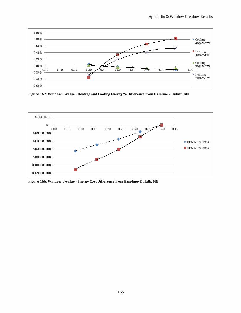
Appendix C: Window U-values Results
166
-0.60%
-0.40%
-0.20%
0.00%
0.20%
0.40%
0.60%
0.80%
1.00%
0.00 0.10 0.20 0.30 0.40 0.50 0.60 0.70 0.80 0.90 1.00
Cooling40% WTW
Heating40% WtW
Cooling70% WTW
Heating70% WTW
Figure 167: Window U-value - Heating and Cooling Energy % Difference from Baseline – Duluth, MN
$(120,000.00)
$(100,000.00)
$(80,000.00)
$(60,000.00)
$(40,000.00)
$(20,000.00)
$-
$20,000.00
0.00 0.05 0.10 0.15 0.20 0.25 0.30 0.35 0.40 0.45
40% WTW Ratio
70% WTW Ratio
Figure 166: Window U-value - Energy Cost Difference from Baseline- Duluth, MN

167
Appendix D: Solar Heat Gain Coefficient Analysis Results
Miami, FL SHGC Results
-40.00%-20.00%
0.00%20.00%40.00%60.00%80.00%
100.00%120.00%140.00%
40%WTW,
SHGC - 0.2
40%WTW,
SHGC - 0.3
40%WTW,
SHGC - 0.4
40%WTW,
SHGC - 0.5
40%WTW,
SHGC - 0.6
70%WTW,
SHGC-0.2
70%WTW,
SHGC-0.3
70%WTW,
SHGC-0.4
70%WTW,
SHGC-0.5
70%WTW,
SHGC-0.6
Occupants (+)
Lights (+)
Equipment (+)
Window (+)
Infiltration )+)
Opaque and other (+)
Window (-)
Infiltration (-)
Figure 169: SHGC - Sensible Heat Gains % Difference from Baseline - Miami, FL
-4000.00
-2000.00
0.00
2000.00
4000.00
6000.00
8000.00
10000.00
12000.00
40%WTW,
SHGC - 0.2
40%WTW,
SHGC - 0.3
40%WTW,
SHGC - 0.4
40%WTW,
SHGC - 0.5
40%WTW,
SHGC - 0.6
70%WTW,
SHGC-0.2
70%WTW,
SHGC-0.3
70%WTW,
SHGC-0.4
70%WTW,
SHGC-0.5
70%WTW,
SHGC-0.6
Heat Rejection
Pumps
Fans
Cooling
Heating
Figure 168: SHGC - Energy Consumption Difference from Baseline - MIami, FL
-50.00%
0.00%
50.00%
100.00%
150.00%
200.00%
250.00%
300.00%
350.00%
0.10 0.20 0.30 0.40 0.50 0.60 0.70
Cooling 40%WTW
Heating 40%WTW
Cooling 70%WTW
Heating 70%WTW
Figure 170: SHGC - Heating and Cooling Energy % Difference from Baseline - Miami, FL

Appendix D: Solar Heat Gain Coefficient Analysis Results
168
Figure 171: SHGC - Energy Cost Savings from Baseline - Miami, FL
Houston, TX SHGC Results
Figure 172: SHGC - Sensible Heat Gains % Difference from Baseline - Houston, TX
Figure 173: SHGC - Energy Consumption Difference from Baseline - Houston, TX
$(50,000.00)
$-
$50,000.00
$100,000.00
$150,000.00
$200,000.00
$250,000.00
0 0.1 0.2 0.3 0.4 0.5 0.6 0.7
40% WTW Ratio
70% WTW Ratio
-40.00%-20.00%
0.00%20.00%40.00%60.00%80.00%
100.00%120.00%140.00%
40%WTW,
SHGC - 0.2
40%WTW,
SHGC - 0.3
40%WTW,
SHGC - 0.4
40%WTW,
SHGC - 0.5
40%WTW,
SHGC - 0.6
70%WTW,
SHGC-0.2
70%WTW,
SHGC-0.3
70%WTW,
SHGC-0.4
70%WTW,
SHGC-0.5
70%WTW,
SHGC-0.6
Occupants (+)
Lights (+)
Equipment (+)
Window (+)
Infiltration )+)
Opaque and other (+)
Window (-)
Infiltration (-)
-2000.00
0.00
2000.00
4000.00
6000.00
8000.00
10000.00
40%WTW,
SHGC - 0.2
40%WTW,
SHGC - 0.3
40%WTW,
SHGC - 0.4
40%WTW,
SHGC - 0.5
40%WTW,
SHGC - 0.6
70%WTW,
SHGC-0.2
70%WTW,
SHGC-0.3
70%WTW,
SHGC-0.4
70%WTW,
SHGC-0.5
70%WTW,
SHGC-0.6
Heat Rejection
Pumps
Fans
Cooling
Heating

Appendix D: Solar Heat Gain Coefficient Analysis Results
169
Figure 174: SHGC - Heating and Cooling Energy % Difference from Baseline - Houston, TX
Figure 175: SHGC - Energy Cost Savings from Baseline - Houston, TX
Phoenix, AZ SHGC Results
Figure 176: SHGC - Sensible Heat Gains % Difference from Baseline - Phoenix, AZ
-20.00%
-10.00%
0.00%
10.00%
20.00%
30.00%
40.00%
50.00%
60.00%
70.00%
0.10 0.20 0.30 0.40 0.50 0.60 0.70
Cooling 40%WTW
Heating 40%WTW
Cooling 70%WTW
Heating 70%WTW
$(50,000.00)
$-
$50,000.00
$100,000.00
$150,000.00
$200,000.00
$250,000.00
0 0.1 0.2 0.3 0.4 0.5 0.6 0.7
40% WTW Ratio
70% WTW Ratio
-50.00%
0.00%
50.00%
100.00%
150.00%
200.00%
40%WTW,
SHGC - 0.2
40%WTW,
SHGC - 0.3
40%WTW,
SHGC - 0.4
40%WTW,
SHGC - 0.5
40%WTW,
SHGC - 0.6
70%WTW,
SHGC-0.2
70%WTW,
SHGC-0.3
70%WTW,
SHGC-0.4
70%WTW,
SHGC-0.5
70%WTW,
SHGC-0.6
Occupants (+)
Lights (+)
Equipment (+)
Window (+)
Infiltration )+)
Opaque and other (+)
Window (-)
Infiltration (-)

Appendix D: Solar Heat Gain Coefficient Analysis Results
170
Figure 177: SHGC - Energy Consumption Difference from Baseline - Phoenix, AZ
Figure 178: SHGC - Heating and Cooling Energy % Difference from Baseline - Phoenix, AZ
Figure 179: SHGC - Energy Cost Savings from Baseline - Phoenix, AZ
-2000.00
-1000.00
0.00
1000.00
2000.00
3000.00
4000.00
5000.00
6000.00
7000.00
8000.00
40%WTW,
SHGC - 0.2
40%WTW,
SHGC - 0.3
40%WTW,
SHGC - 0.4
40%WTW,
SHGC - 0.5
40%WTW,
SHGC - 0.6
70%WTW,
SHGC-0.2
70%WTW,
SHGC-0.3
70%WTW,
SHGC-0.4
70%WTW,
SHGC-0.5
70%WTW,
SHGC-0.6
Heat Rejection
Pumps
Fans
Cooling
Heating
-10.00%
-5.00%
0.00%
5.00%
10.00%
15.00%
20.00%
25.00%
30.00%
35.00%
0.10 0.20 0.30 0.40 0.50 0.60 0.70
Cooling40% WTW
Heating40% WTW
Cooling70% WTW
Heating70% WTW
$(40,000.00)
$(20,000.00)
$-
$20,000.00
$40,000.00
$60,000.00
$80,000.00
$100,000.00
$120,000.00
$140,000.00
$160,000.00
0 0.1 0.2 0.3 0.4 0.5 0.6 0.7
40% WTW Ratio
70% WTW Ratio

Appendix D: Solar Heat Gain Coefficient Analysis Results
171
San Francisco, CA SHGC Results
Figure 180: SHGC - Sensible Heat Gains % Difference from Baseline - San Francisco, CA
Figure 181: SHGC - Energy Consumption Difference from Baseline - San Francisco, CA
-50.00%
0.00%
50.00%
100.00%
150.00%
200.00%
250.00%
40%WTW,
SHGC - 0.2
40%WTW,
SHGC - 0.3
40%WTW,
SHGC - 0.4
40%WTW,
SHGC - 0.5
40%WTW,
SHGC - 0.6
70%WTW,
SHGC-0.2
70%WTW,
SHGC-0.3
70%WTW,
SHGC-0.4
70%WTW,
SHGC-0.5
70%WTW,
SHGC-0.6
Occupants (+)
Lights (+)
Equipment (+)
Window (+)
Infiltration )+)
Opaque and other (+)
Window (-)
Infiltration (-)
-2000.00
0.00
2000.00
4000.00
6000.00
8000.00
10000.00
40%WTW,
SHGC - 0.2
40%WTW,
SHGC - 0.3
40%WTW,
SHGC - 0.4
40%WTW,
SHGC - 0.5
40%WTW,
SHGC - 0.6
70%WTW,
SHGC-0.2
70%WTW,
SHGC-0.3
70%WTW,
SHGC-0.4
70%WTW,
SHGC-0.5
70%WTW,
SHGC-0.6
Heat Rejection
Pumps
Fans
Cooling
Heating

Appendix D: Solar Heat Gain Coefficient Analysis Results
172
Figure 182: SHGC - Heating and Cooling Energy % Difference from Baseline - San Francisco, CA
Figure 183: SHGC - Energy Cost Savings from Baseline - San Francisco, CA
Baltimore, MD SGHC Results
Figure 184: SHGC - Sensible Heat Gains % Difference from Baseline - Baltimore, MD
-40.00%
-20.00%
0.00%
20.00%
40.00%
60.00%
80.00%
100.00%
120.00%
140.00%
160.00%
0.10 0.20 0.30 0.40 0.50 0.60 0.70
Cooling 40%WTW
Heating 40%WTW
Cooling 70%WTW
Heating 70%WTW
$(100,000.00)
$(50,000.00)
$-
$50,000.00
$100,000.00
$150,000.00
$200,000.00
$250,000.00
$300,000.00
0 0.1 0.2 0.3 0.4 0.5 0.6 0.7
40% WTW Ratio
70% WTW Ratio
-60.00%
-40.00%
-20.00%
0.00%
20.00%
40.00%
60.00%
80.00%
40%WTW,
SHGC - 0.2
40%WTW,
SHGC - 0.3
40%WTW,
SHGC - 0.4
40%WTW,
SHGC - 0.5
40%WTW,
SHGC - 0.6
70%WTW,
SHGC-0.2
70%WTW,
SHGC-0.3
70%WTW,
SHGC-0.4
70%WTW,
SHGC-0.5
70%WTW,
SHGC-0.6
Occupants (+)
Lights (+)
Equipment (+)
Window (+)
Infiltration )+)
Opaque and other (+)
Window (-)
Infiltration (-)

Appendix D: Solar Heat Gain Coefficient Analysis Results
173
Figure 185: SHGC - Energy Consumption Difference from Baseline - Baltimore, MD
Figure 186: SHGC - Heating and Cooling Energy % Difference from Baseline - Baltimore, MD
Figure 187: SHGC - Energy Cost Savings from Baseline - Baltimore, MD
-3000.00
-2000.00
-1000.00
0.00
1000.00
2000.00
3000.00
4000.00
5000.00
40%WTW,
SHGC - 0.2
40%WTW,
SHGC - 0.3
40%WTW,
SHGC - 0.4
40%WTW,
SHGC - 0.5
40%WTW,
SHGC - 0.6
70%WTW,
SHGC-0.2
70%WTW,
SHGC-0.3
70%WTW,
SHGC-0.4
70%WTW,
SHGC-0.5
70%WTW,
SHGC-0.6
Heat Rejection
Pumps
Fans
Cooling
Heating
-20.00%
-15.00%
-10.00%
-5.00%
0.00%
5.00%
10.00%
15.00%
20.00%
25.00%
0.10 0.20 0.30 0.40 0.50 0.60 0.70
Cooling 40%WTW
Heating 40%WTW
Cooling 70%WTW
Heating 70%WTW
$(60,000.00)
$(40,000.00)
$(20,000.00)
$-
$20,000.00
$40,000.00
$60,000.00
$80,000.00
0 0.1 0.2 0.3 0.4 0.5 0.6 0.7
40% WTW Ratio
70% WTW Ratio

Appendix D: Solar Heat Gain Coefficient Analysis Results
174
Seattle, WA SHGC Results
Figure 188: SHGC - Sensible Heat Gains % Difference from Baseline - Seattle, WA
Figure 189: SHGC - Energy Consumption Difference from Baseline - Seattle, WA
Figure 190: SHGC - Heating and Cooling Energy % Difference from Baseline – Seattle, WA
-80.00%-60.00%-40.00%-20.00%
0.00%20.00%40.00%60.00%80.00%
100.00%
40%WTW,
SHGC - 0.2
40%WTW,
SHGC - 0.3
40%WTW,
SHGC - 0.4
40%WTW,
SHGC - 0.5
40%WTW,
SHGC - 0.6
70%WTW,
SHGC-0.2
70%WTW,
SHGC-0.3
70%WTW,
SHGC-0.4
70%WTW,
SHGC-0.5
70%WTW,
SHGC-0.6
Occupants (+)
Lights (+)
Equipment (+)
Window (+)
Infiltration )+)
Opaque and other (+)
Window (-)
Infiltration (-)
-5000.00
-4000.00
-3000.00
-2000.00
-1000.00
0.00
1000.00
2000.00
3000.00
4000.00
5000.00
6000.00
40%WTW,
SHGC - 0.2
40%WTW,
SHGC - 0.3
40%WTW,
SHGC - 0.4
40%WTW,
SHGC - 0.5
40%WTW,
SHGC - 0.6
70%WTW,
SHGC-0.2
70%WTW,
SHGC-0.3
70%WTW,
SHGC-0.4
70%WTW,
SHGC-0.5
70%WTW,
SHGC-0.6
Heat Rejection
Pumps
Fans
Cooling
Heating
-30.00%
-20.00%
-10.00%
0.00%
10.00%
20.00%
30.00%
40.00%
50.00%
0.10 0.20 0.30 0.40 0.50 0.60 0.70
Cooling 40%WTW
Heating 40%WTW
Cooling 70%WTW
Heating 70%WTW

Appendix D: Solar Heat Gain Coefficient Analysis Results
175
Figure 191: SHGC - Energy Cost Savings from Baseline – Seattle, WA
Chicago, IL SHGC Results
Figure 192: SHGC - Sensible Heat Gains % Difference from Baseline - Chicago, IL
Figure 193: SHGC - Energy Consumption Difference from Baseline - Chicago, IL
$(80,000.00)
$(60,000.00)
$(40,000.00)
$(20,000.00)
$-
$20,000.00
$40,000.00
$60,000.00
$80,000.00
$100,000.00
0 0.1 0.2 0.3 0.4 0.5 0.6 0.7
40% WTW Ratio
70% WTW Ratio
-100.00%
-50.00%
0.00%
50.00%
100.00%
150.00%
200.00%
250.00%
40%WTW,
SHGC-0.2
40%WTW,
SHGC-0.3
40%WTW,
SHGC-0.4
40%WTW,
SHGC-0.5
40%WTW,
SHGC-0.6
70%WTW,
SHGC-0.2
70%WTW,
SHGC-0.3
70%WTW,
SHGC-0.4
70%WTW,
SHGC-0.5
70%WTW,
SHGC-0.6
Occupants (+)
Lights (+)
Equipment (+)
Window (+)
Infiltration )+)
Opaque and other (+)
Window (-)
Infiltration (-)
-3000.00
-2000.00
-1000.00
0.00
1000.00
2000.00
3000.00
4000.00
40%WTW,
SHGC-0.2
40%WTW,
SHGC-0.3
40%WTW,
SHGC-0.4
40%WTW,
SHGC-0.5
40%WTW,
SHGC-0.6
70%WTW,
SHGC-0.2
70%WTW,
SHGC-0.3
70%WTW,
SHGC-0.4
70%WTW,
SHGC-0.5
70%WTW,
SHGC-0.6
Heat Rejection
Pumps
Fans
Cooling
Heating

Appendix D: Solar Heat Gain Coefficient Analysis Results
176
Figure 194: SHGC - Heating and Cooling Energy % Difference from Baseline - Chicago, IL
Figure 195: SHGC - Energy Cost Savings from Baseline - Chicago, IL
Denver, CO SHGC Results
Figure 196: SHGC - Sensible Heat Gains % Difference from Baseline - Denver, CO
-20.00%
-15.00%
-10.00%
-5.00%
0.00%
5.00%
10.00%
15.00%
20.00%
25.00%
0.10 0.20 0.30 0.40 0.50 0.60 0.70
Cooling 40%WTW
Heating 40%WTW
Cooling 70%WTW
Heating 70%WTW
$(60,000.00)
$(40,000.00)
$(20,000.00)
$-
$20,000.00
$40,000.00
$60,000.00
$80,000.00
0 0.1 0.2 0.3 0.4 0.5 0.6 0.7
40% WTW Ratio
70% WTW Ratio
-60.00%
-40.00%
-20.00%
0.00%
20.00%
40.00%
60.00%
80.00%
40%WTW,
SHGC - 0.2
40%WTW,
SHGC - 0.3
40%WTW,
SHGC - 0.4
40%WTW,
SHGC - 0.5
40%WTW,
SHGC - 0.6
70%WTW,
SHGC-0.2
70%WTW,
SHGC-0.3
70%WTW,
SHGC-0.4
70%WTW,
SHGC-0.5
70%WTW,
SHGC-0.6
Occupants (+)
Lights (+)
Equipment (+)
Window (+)
Infiltration )+)
Opaque and other (+)
Window (-)
Infiltration (-)

Appendix D: Solar Heat Gain Coefficient Analysis Results
177
Figure 197: SHGC - Energy Consumption Difference from Baseline - Denver, CO
Figure 198: SHGC - Heating and Cooling Energy % Difference from Baseline - Denver, CO
Figure 199: SHGC - Energy Cost Savings from Baseline - Denver, CO
-3000.00
-2000.00
-1000.00
0.00
1000.00
2000.00
3000.00
4000.00
40%WTW,
SHGC - 0.2
40%WTW,
SHGC - 0.3
40%WTW,
SHGC - 0.4
40%WTW,
SHGC - 0.5
40%WTW,
SHGC - 0.6
70%WTW,
SHGC-0.2
70%WTW,
SHGC-0.3
70%WTW,
SHGC-0.4
70%WTW,
SHGC-0.5
70%WTW,
SHGC-0.6
Heat Rejection
Pumps
Fans
Cooling
Heating
-25.00%
-20.00%
-15.00%
-10.00%
-5.00%
0.00%
5.00%
10.00%
15.00%
20.00%
25.00%
30.00%
0.10 0.20 0.30 0.40 0.50 0.60 0.70
Cooling 40%WTW
Heating 40%WTW
Cooling 70%WTW
Heating 70%WTW
$(30,000.00)
$(20,000.00)
$(10,000.00)
$-
$10,000.00
$20,000.00
$30,000.00
$40,000.00
0 0.1 0.2 0.3 0.4 0.5 0.6 0.7
40% WTW Ratio
70% WTW Ratio

Appendix D: Solar Heat Gain Coefficient Analysis Results
178
Helena, MT SHGC Results
Figure 200: SHGC - Sensible Heat Gains % Difference from Baseline - Helena, MT
Figure 201: SHGC - Energy Consumption Difference from Baseline - Helena, MT
Figure 202: SHGC - Heating and Cooling Energy % Difference from Baseline - Helena, MT
-80.00%-60.00%-40.00%-20.00%
0.00%20.00%40.00%60.00%80.00%
100.00%
40%WTW,
SHGC - 0.2
40%WTW,
SHGC - 0.3
40%WTW,
SHGC - 0.4
40%WTW,
SHGC - 0.5
40%WTW,
SHGC - 0.6
70%WTW,
SHGC-0.2
70%WTW,
SHGC-0.3
70%WTW,
SHGC-0.4
70%WTW,
SHGC-0.5
70%WTW,
SHGC-0.6
Occupants (+)
Lights (+)
Equipment (+)
Window (+)
Infiltration )+)
Opaque and other (+)
Window (-)
Infiltration (-)
-2000.00
-1500.00
-1000.00
-500.00
0.00
500.00
1000.00
1500.00
2000.00
2500.00
3000.00
40%WTW,
SHGC - 0.2
40%WTW,
SHGC - 0.3
40%WTW,
SHGC - 0.4
40%WTW,
SHGC - 0.5
40%WTW,
SHGC - 0.6
70%WTW,
SHGC-0.2
70%WTW,
SHGC-0.3
70%WTW,
SHGC-0.4
70%WTW,
SHGC-0.5
70%WTW,
SHGC-0.6
Heat Rejection
Pumps
Fans
Cooling
Heating
-30.00%
-20.00%
-10.00%
0.00%
10.00%
20.00%
30.00%
0.10 0.20 0.30 0.40 0.50 0.60 0.70
Cooling 40%WTW
Heating 40%WTW
Cooling 70%WTW
Heating 70%WTW

Appendix D: Solar Heat Gain Coefficient Analysis Results
179
Figure 203: SHGC - Energy Cost Savings from Baseline - Helena, MT
Duluth, MN SHGC Results
Figure 204: SHGC - Sensible Heat Gains % Difference from Baseline - Duluth, MN
Figure 205: SHGC - Energy Consumption Difference from Baseline - Duluth, MN
$(40,000.00)
$(30,000.00)
$(20,000.00)
$(10,000.00)
$-
$10,000.00
$20,000.00
$30,000.00
$40,000.00
$50,000.00
$60,000.00
$70,000.00
0 0.1 0.2 0.3 0.4 0.5 0.6 0.7
40% WTW Ratio
70% WTW Ratio
-80.00%
-60.00%
-40.00%
-20.00%
0.00%
20.00%
40.00%
60.00%
40%WTW,
SHGC - 0.2
40%WTW,
SHGC - 0.3
40%WTW,
SHGC - 0.4
40%WTW,
SHGC - 0.5
40%WTW,
SHGC - 0.6
70%WTW,
SHGC-0.2
70%WTW,
SHGC-0.3
70%WTW,
SHGC-0.4
70%WTW,
SHGC-0.5
70%WTW,
SHGC-0.6
Occupants (+)
Lights (+)
Equipment (+)
Window (+)
Infiltration )+)
Opaque and other (+)
Window (-)
Infiltration (-)
-3000.00
-2000.00
-1000.00
0.00
1000.00
2000.00
3000.00
40%WTW,
SHGC - 0.2
40%WTW,
SHGC - 0.3
40%WTW,
SHGC - 0.4
40%WTW,
SHGC - 0.5
40%WTW,
SHGC - 0.6
70%WTW,
SHGC-0.2
70%WTW,
SHGC-0.3
70%WTW,
SHGC-0.4
70%WTW,
SHGC-0.5
70%WTW,
SHGC-0.6
Heat Rejection
Pumps
Fans
Cooling
Heating
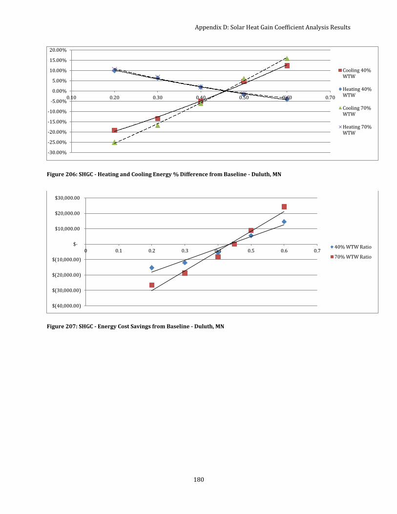
Appendix D: Solar Heat Gain Coefficient Analysis Results
180
Figure 206: SHGC - Heating and Cooling Energy % Difference from Baseline - Duluth, MN
Figure 207: SHGC - Energy Cost Savings from Baseline - Duluth, MN
-30.00%
-25.00%
-20.00%
-15.00%
-10.00%
-5.00%
0.00%
5.00%
10.00%
15.00%
20.00%
0.10 0.20 0.30 0.40 0.50 0.60 0.70
Cooling 40%WTW
Heating 40%WTW
Cooling 70%WTW
Heating 70%WTW
$(40,000.00)
$(30,000.00)
$(20,000.00)
$(10,000.00)
$-
$10,000.00
$20,000.00
$30,000.00
0 0.1 0.2 0.3 0.4 0.5 0.6 0.740% WTW Ratio
70% WTW Ratio

Appendix E: Visible Transmittance Analysis Results
181
Appendix E: Visible Transmittance Analysis Results
Miami, FL Visible Transmittance Results
Houston, TX Visible Transmittance Results
-250.00
-200.00
-150.00
-100.00
-50.00
0.00
50.00
100.00
40% WTW,VT-0.3
40% WTW,VT-0.5
40% WTW,VT-0.7
40% WTW,VT-0.9
70% WTW,VT-0.3
70% WTW,VT-0.5
70% WTW,VT-0.7
70% WTW,VT-0.9
En
erg
y C
on
sum
pti
on
D
iffe
ren
ce f
rom
Ba
seli
ne
(G
J)
Heat Rejection
Pumps
Fans
Cooling
Heating
$(30,000.00)
$(25,000.00)
$(20,000.00)
$(15,000.00)
$(10,000.00)
$(5,000.00)
$-
$5,000.00
0.00 0.20 0.40 0.60 0.80 1.00
Visible Transmittance
40% WTW Ratio
70% WTW Ratio
Figure 208: Visible Transmittance - Annual Energy Consumption Difference from Daylight Baseline - Miami, FL
Figure 209: Visible Transmittance - Annual Energy Cost Difference from Daylight Baseline - Miami, FL
-150.00
-100.00
-50.00
0.00
50.00
100.00
150.00
40% WTW,VT-0.3
40% WTW,VT-0.5
40% WTW,VT-0.7
40% WTW,VT-0.9
70% WTW,VT-0.3
70% WTW,VT-0.5
70% WTW,VT-0.7
70% WTW,VT-0.9
En
erg
y C
on
sum
pti
on
D
iffe
ren
ce f
rom
Ba
seli
n (
GJ)
Heat Rejection
Pumps
Fans
Cooling
Heating
Figure 210: Visible Transmittance - Annual Energy Consumption Difference from Daylight Baseline - Houston, TX

Appendix E: Visible Transmittance Analysis Results
182
Figure 211: Visible Transmittance - Annual Energy Cost Difference from Daylight Baseline - Houston, TX
Phoenix, AZ Visible Transmittance Results
Figure 212: Visible Transmittance - Annual Energy Consumption Difference from Daylight Baseline - Phoenix, AZ
$(30,000.00)
$(25,000.00)
$(20,000.00)
$(15,000.00)
$(10,000.00)
$(5,000.00)
$-
0.000 0.100 0.200 0.300 0.400 0.500 0.600 0.700 0.800 0.900 1.000
Visible Transmittance
40% WTW Ratio
70% WTW Ratio
-150.00
-100.00
-50.00
0.00
50.00
100.00
150.00
40% WTW,VT-0.3
40% WTW,VT-0.5
40% WTW,VT-0.7
40% WTW,VT-0.9
70% WTW,VT-0.3
70% WTW,VT-0.5
70% WTW,VT-0.7
70% WTW,VT-0.9
En
erg
y C
on
sum
pti
on
D
iffe
ren
ce f
rom
Ba
seli
ne
(G
J)
Heat Rejection
Pumps
Fans
Cooling
Heating
$(25,000.00)
$(20,000.00)
$(15,000.00)
$(10,000.00)
$(5,000.00)
$-
0.000 0.100 0.200 0.300 0.400 0.500 0.600 0.700 0.800 0.900 1.000
Visible Transmittance
40% WTW Ratio
70% WTW Ratio

Appendix E: Visible Transmittance Analysis Results
183
Atlanta, GA Visible Transmittance Results
Figure 213: Visible Transmittance - Annual Energy Consumption Difference from Daylight Baseline - Atlanta, GA
Figure 214: Visible Transmittance - Annual Energy Cost Difference from Daylight Baseline - Atlanta, GA
San Francisco, CA Visible Transmittance Results
Figure 215: Visible Transmittance - Annual Energy Consumption Difference from Daylight Baseline - San
Francisco, CA
-150.00
-100.00
-50.00
0.00
50.00
100.00
150.00
200.00
40% WTW,VT-0.3
40% WTW,VT-0.5
40% WTW,VT-0.7
40% WTW,VT-0.9
70% WTW,VT-0.3
70% WTW,VT-0.5
70% WTW,VT-0.7
70% WTW,VT-0.9
Heat Rejection
Pumps
Fans
Cooling
Heating
$(14,000.00)
$(12,000.00)
$(10,000.00)
$(8,000.00)
$(6,000.00)
$(4,000.00)
$(2,000.00)
$-
0.00 0.10 0.20 0.30 0.40 0.50 0.60 0.70 0.80 0.90 1.00
Visible Transmittance
40% WTW Ratio
70% WTW Ratio
-100.00
-50.00
0.00
50.00
100.00
150.00
200.00
40% WTW,VT-0.3
40% WTW,VT-0.5
40% WTW,VT-0.7
40% WTW,VT-0.9
70% WTW,VT-0.3
70% WTW,VT-0.5
70% WTW,VT-0.7
70% WTW,VT-0.9
Heat Rejection
Pumps
Fans
Cooling
Heating

Appendix E: Visible Transmittance Analysis Results
184
Baltimore, MD Visible Transmittance Results
Figure 216: Visible Transmittance - Annual Energy Consumption Difference from Daylight Baseline - Baltimore,
MD
Figure 217: Visible Transmittance - Annual Energy Cost Difference from Daylight Baseline - Baltimore, MD
$(30,000.00)
$(25,000.00)
$(20,000.00)
$(15,000.00)
$(10,000.00)
$(5,000.00)
$-
0.00 0.10 0.20 0.30 0.40 0.50 0.60 0.70 0.80 0.90 1.00
Visible Transmittance
40% WTW Ratio
70% WTW Ratio
-40.00
-20.00
0.00
20.00
40.00
60.00
80.00
100.00
120.00
40% WTW,VT-0.3
40% WTW,VT-0.5
40% WTW,VT-0.7
40% WTW,VT-0.9
70% WTW,VT-0.3
70% WTW,VT-0.5
70% WTW,VT-0.7
70% WTW,VT-0.9
Heat Rejection
Pumps
Fans
Cooling
Heating
$(8,000.00)
$(7,000.00)
$(6,000.00)
$(5,000.00)
$(4,000.00)
$(3,000.00)
$(2,000.00)
$(1,000.00)
$-
$1,000.00
$2,000.00
0.000 0.100 0.200 0.300 0.400 0.500 0.600 0.700 0.800 0.900 1.000
Visible Transmittance
40% WTW Ratio
70% WTW Ratio

Appendix E: Visible Transmittance Analysis Results
185
Seattle, WA Visible Transmittance Results
Figure 218: Visible Transmittance - Annual Energy Consumption Difference from Daylight Baseline - Seattle, WA
Figure 219: Visible Transmittance - Annual Energy Cost Difference from Daylight Baseline - Seattle, WA
Chicago, IL Visible Transmittance Results
Figure 220: Visible Transmittance - Annual Energy Consumption Difference from Daylight Baseline - Chicago, IL
-50.00
0.00
50.00
100.00
150.00
200.00
250.00
40% WTW,VT-0.3
40% WTW,VT-0.5
40% WTW,VT-0.7
40% WTW,VT-0.9
70% WTW,VT-0.3
70% WTW,VT-0.5
70% WTW,VT-0.7
70% WTW,VT-0.9
Heat Rejection
Pumps
Fans
Cooling
Heating
$(4,000.00)
$(3,500.00)
$(3,000.00)
$(2,500.00)
$(2,000.00)
$(1,500.00)
$(1,000.00)
$(500.00)
$-
$500.00
$1,000.00
0.000 0.100 0.200 0.300 0.400 0.500 0.600 0.700 0.800 0.900 1.000
Visible Transmittance
40% WTW Ratio
70% WTW Ratio
-40
-20
0
20
40
60
80
100
120
140
160
40% WTW,VT-0.3
40% WTW,VT-0.5
40% WTW,VT-0.7
40% WTW,VT-0.9
70% WTW,VT-0.3
70% WTW,VT-0.5
70% WTW,VT-0.7
70% WTW,VT-0.9
Heat Rejection
Pumps
Fans
Cooling
Heating

Appendix E: Visible Transmittance Analysis Results
186
Figure 221: Visible Transmittance - Annual Energy Cost Difference from Daylight Baseline - Chicago, IL
Denver, CO Visible Transmittance Results
Figure 222: Visible Transmittance - Annual Energy Consumption Difference from Daylight Baseline - Denver, CO
Figure 223: Visible Transmittance - Annual Energy Cost Difference from Daylight Baseline - Denver, CO
$(4,500.00)
$(4,000.00)
$(3,500.00)
$(3,000.00)
$(2,500.00)
$(2,000.00)
$(1,500.00)
$(1,000.00)
$(500.00)
$-
$500.00
$1,000.00
0.000 0.100 0.200 0.300 0.400 0.500 0.600 0.700 0.800 0.900 1.000
Visible Transmittance
40% WTW Ratio
70% WTW Ratio
-40.00
-20.00
0.00
20.00
40.00
60.00
80.00
100.00
120.00
40% WTW,VT-0.3
40% WTW,VT-0.5
40% WTW,VT-0.7
40% WTW,VT-0.9
70% WTW,VT-0.3
70% WTW,VT-0.5
70% WTW,VT-0.7
70% WTW,VT-0.9
Heat Rejection
Pumps
Fans
Cooling
Heating
$(2,000.00)
$(1,500.00)
$(1,000.00)
$(500.00)
$-
$500.00
0.000 0.100 0.200 0.300 0.400 0.500 0.600 0.700 0.800 0.900 1.000
Visible Transmittance
40% WTW Ratio
70% WTW Ratio

Appendix E: Visible Transmittance Analysis Results
187
Helena, MT Visible Transmittance Results
Figure 224: Visible Transmittance - Annual Energy Consumption Difference from Daylight Baseline - Helena, MT
Figure 225: Visible Transmittance - Annual Energy Cost Difference from Daylight Baseline - Helena, MT
Duluth, MN Visible Transmittance Results
Figure 226: Visible Transmittance - Annual Energy Consumption Difference from Daylight Baseline - Duluth, MN
-40.00-20.00
0.0020.0040.0060.0080.00
100.00120.00140.00160.00180.00
40% WTW,VT-0.3
40% WTW,VT-0.5
40% WTW,VT-0.7
40% WTW,VT-0.9
70% WTW,VT-0.3
70% WTW,VT-0.5
70% WTW,VT-0.7
70% WTW,VT-0.9
Heat Rejection
Pumps
Fans
Cooling
Heating
$(4,500.00)
$(4,000.00)
$(3,500.00)
$(3,000.00)
$(2,500.00)
$(2,000.00)
$(1,500.00)
$(1,000.00)
$(500.00)
$-
$500.00
$1,000.00
0.000 0.100 0.200 0.300 0.400 0.500 0.600 0.700 0.800 0.900 1.000
Visible Transmittance
40% WTW Ratio
70% WTW Ratio
-100.00
-50.00
0.00
50.00
100.00
150.00
200.00
40% WTW,VT-0.3
40% WTW,VT-0.5
40% WTW,VT-0.7
40% WTW,VT-0.9
70% WTW,VT-0.3
70% WTW,VT-0.5
70% WTW,VT-0.7
70% WTW,VT-0.9
Heat Rejection
Pumps
Fans
Cooling
Heating
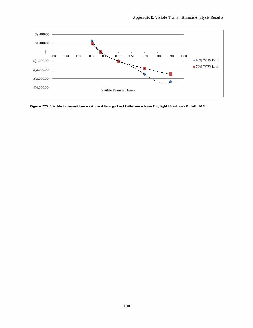
Appendix E: Visible Transmittance Analysis Results
188
Figure 227: Visible Transmittance - Annual Energy Cost Difference from Daylight Baseline - Duluth, MN
$(4,000.00)
$(3,000.00)
$(2,000.00)
$(1,000.00)
$-
$1,000.00
$2,000.00
0.00 0.10 0.20 0.30 0.40 0.50 0.60 0.70 0.80 0.90 1.00
Visible Transmittance
40% WTW Ratio
70% WTW Ratio

189
Appendix F: Window Properties for Highest and Lowest Ten Energy
Consumers
Figure 228: Window Properties for Highest and Lowest Ten Energy Consumers - Miami, FL
Figure 229: Window Properties for Highest and Lowest Ten Energy Consumers - Houston, TX

Appendix F: Window Properties for Highest and Lowest Ten Energy Consumers
190
Figure 230: Window Properties for Highest and Lowest Ten Energy Consumers - Phoenix, AZ
Figure 231: Window Properties for Highest and Lowest Ten Energy Consumers - Atlanta, GA

Appendix F: Window Properties for Highest and Lowest Ten Energy Consumers
191
Figure 232: Window Properties for Highest and Lowest Ten Energy Consumers - San Francisco, CA
Figure 233: Window Properties for Highest and Lowest Ten Energy Consumers - Baltimore, MD

Appendix F: Window Properties for Highest and Lowest Ten Energy Consumers
192
Figure 234: Window Properties for Highest and Lowest Ten Energy Consumers - Seattle, WA
Figure 235: Window Properties for Highest and Lowest Ten Energy Consumers - Chicago, IL

Appendix F: Window Properties for Highest and Lowest Ten Energy Consumers
193
Figure 236: Window Properties for Highest and Lowest Ten Energy Consumers - Denver, CO
Figure 237: Window Properties for Highest and Lowest Ten Energy Consumers - Helena, MT

Appendix F: Window Properties for Highest and Lowest Ten Energy Consumers
194
Figure 238: Window Properties for Highest and Lowest Ten Energy Consumers - Duluth, MN

195