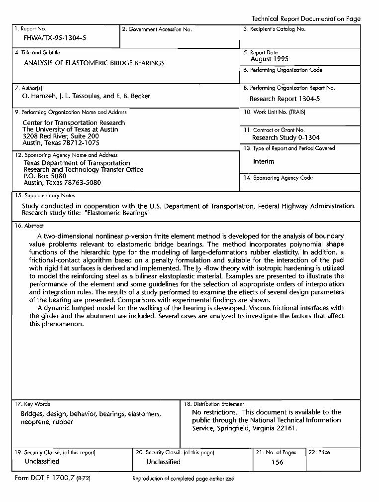
Technical Report Documentation Page

1 . Report No. 2. Government Accession No. 3. Recipient's Catalog No.

FHWA/TX-95-1 304-5

4. Title and Subtitle

ANALYSIS OF ELASTOMERIC BRIDGE BEARINGS

7. Author[sJ 0. Hamzeh, J. L. Tassoulas, and E. B. Becker

9. Performing Organization Name and Address

Center for Transportation Research

5. Report Date August 1995

6. Performing Organization Code

8. Performing Organization Report No.

Research Report 1 304-5

1 0. Work Unit No. [TRAISJ

The University of Texas at Austin 11. Contract or Grant No. 3208 Red River, Suite 200 Research Study 0-1 304 Austin, Texas 78712-1075

t-:-:--:----:---:-----:-~-:------------------l 13. Type of Report and Period Covered 12. Sponsoring Agency Name and Address

Texas Department of Transportation Research and Technology Transfer Office P.O. Box 5080 Austin, Texas 78763-5080

15. Supplementary Notes

Interim

14. Sponsoring Agency Code

Study conducted in cooperation with the U.S. Department of Transportation, Federal Highway Administration. Research study title: "Eiastomeric Bearings"

16. Abstract

A two-dimensional nonlinear p-version finite element method is developed for the analysis of boundary value problems relevant to elastomeric bridge bearings. The method incorporates polynomial shape functions of the hierarchic type for the modeling of large-deformations rubber elasticity. ·In addition, a frictional-contact algorithm based on a penalty formulation and suitable for the interaction of the pad with rigid flat surfaces is derived and implemented. The J2 -flow theory with isotropic hardening is utilized to model the reinforcing steel as a bilinear elastoplastic material. Examples are presented to illustrate the performance of the element and some guidelines for the selection of appropriate orders of interpolation and integration rules. The results of a study performed to examine the effects of several design parameters of the bearing are presented. Comparisons with experimental findings are shown.

A dynamic lumped model for the walking of the bearing is developed. Viscous frictional interfaces with the girder and the abutment are included. Several cases are analyzed to investigate the factors that affect this phenomenon.

17. Key Words 1 8. Distribution Statement

Bridges, design, behavior, bearings, elastomers, neoprene, rubber

No restrictions. This document is available to the public through the National Technical Information Service, Springfield, Virginia 221 61 .

19. Security Classif. [of this report)

Unclassified

Form DOT F 1700.7 (8-72)

20. Security Classif. [of this page)

Unclassified

Reproduction of completed page authorized

21 . No. of Pages

156

22. Price

ANALYSIS OF ELASTOMERIC BRIDGE BEARINGS

by

O.Hamzeh J. L. Tassoulas

and E. B. Becker

Research Report Number 1304-5

Research Project 0-1304 Elastomeric Bearings

conducted for the

TEXAS DEPARTMENT OF TRANSPORTATION

in cooperation with the

U.S. Department of Transportation Federal Highway Administration

by the

CENTER FOR TRANSPORTATION RESEARCH Bureau of Engineering Research

THE UNIVERSITY OF TEXAS AT AUSTIN

August 1995

IMPLEMENTATION

Use of the computational procedure described in this report permits estimation of the shear and compressive stiffnesses of elastomeric bridge bearings. The procedure is applicable to plain as well as steel-reinforced pads, flat or tapered. In addition to the stiffnesses, estimates of stress and deformation levels in the bearings are obtained. The results of application of the procedure indicate that neither the stiffnesses nor the levels of stress and deformation are affected significantly by the taper of the pad.

The report also addresses the phenomenon of bearing movement ("walking"). By means of analysis of a simple model, the movement is linked to the loss of adhesion and increase in smoothness at the pad-girder and pad-abutment interfaces in the presence of the waxy substance that is added to rubber as a protectant and is exuded to the pad surfaces.

Prepared in cooperation with the Texas Department of Transportation and the U.S. Department of Transportation, Federal Highway Administration.

The contents of this report reflect the views of the authors, who are responsible for the facts and the accuracy of the data presented herein. The contents do not necessarily reflect the official view or policies of the Federal Highway Administration or the Texas Department of Transportation. This report does not constitute a standard, specification, or regulation.

NO INTENDED FOR CONSTRUCTION, BIDDING, OR PERMIT PURPOSES

John L. Tassoulas, P.E. #71599 Eric B. Becker, P.E. #78854

Research Supervisors

Ill

TABLE OF CONTENTS

Chapter 1-11\ITRODUCTION ..................................................................................... 1

1.1 Elastomeric Bearings............................................................................ 1

1.2 State of the Art . . . . . . . . . . . . . . . . . . . . . . . . . . . . . . . . . . . . . . . . . .. . . . . . . . . . . . . . . . . . . . . . . . . . . .. .. . . . . . . . . . . . . 5

1.2.1 Methods of Analysis.................................................................. 5

1.2.2 Finite Element Adaptive Methods: the p-version ... . . . .. . . . . . .. . ...... 6

1.2.3 Contact Algorithms .................................................................... 12

1.3 Objective............................................................................................... 13

Chapter 2- P-VERSION FINITE ELEMENT METHOD ............................................. 14

2.1 Introduction ........................................................................................... 14

2.2 Large-Deformation Kinematics ............................................................. 14

2.3 Hyperelastic Incompressible Materials .................................................. 19

2.4 Problem Statement.. ............................................................................. 20

2.5 Finite Element Discretization ................................................................ 21

2.6 Displacement Interpolation ................................................................... 24

2.6.1 Comer Modes ........................................................................... 24

2.6.2 Side Modes ............................................................................... 24

2.6.3 Internal Modes .......................................................................... 26

2. 7 Pressure Interpolation .......................................................................... 28

2.8 Order of Interpolations .......................................................................... 28

2.9 Numerical Integration ............................................................................ 31

v

Chapter 3- FRICTIONAL-CONTACT ALGORITHM .................................................. 33

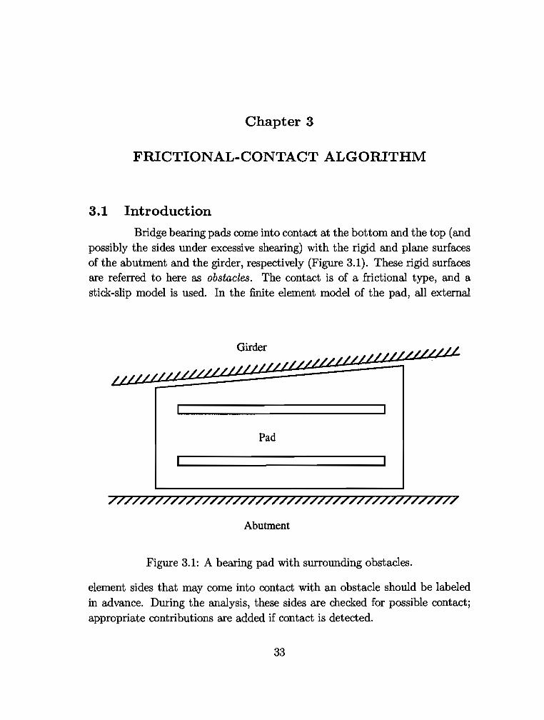
3.1 Introduction .......................................................................................... 33

3.2 Frictional Contact at a Point by Penalty Formulation ............................ 34

3.3 Contact Contribution to the Virtual Work .............................................. 36

3.4 Contact Contribution to the Finite Element Equations.......................... 39

3.5 Practical Considerations....................................................................... 40

Chapter 4- EXAMPLES AND APPLICATIONS ........................................................ 42

4.1 Introduction .......................................................................................... 42

4.2 Performance of the Higher-Order Element........................................... 42

4.2.1 Comparisons with the Quadratic Element.. ............................... 43

4.2.2 Order of Pressure Interpolation ................................................. 44

4.2.3 Order of Integration Rule .......................................................... 51

4.3 Bridge Bearing Pads ............................................................................ 51

4.3.1 Preliminary Notes ...................................................................... 53

4.3.2 General Observations............................................................... 56

4.3.3 FXO in Tapered Pads ................................................................ 63

4.3.4 Effect of Some Design Factors ................................................. 69

4.3.4.1 Compressive Load, FY ................................................ 70

4.3.4.2 Shear Modulus of Rubber, G ....................................... 71

4.3.4.3 Flat vs. Tapered Pads .................................................. 71

4.3.4.4 Number of Steel Laminates ......................................... 72

4.3.4.5 Thickness of Steel Laminates ...................................... 72

4.3.4.6 Positioning of Steel Laminates (horizontal vs. radial) in Tapered Pads .......................................................... 72

4.3.4.7 Other Results ............................................................... 73

VI

4.3.5 Analysis ..................................................................................... 74

4.3.5.1 Compressive Stiffness of the Pad, Kcomp ...................... 7 4

4.3.5.2 Shear Stiffness of the Pad, Kshear··· .............................. 75

4.3.5.3 Effect of Shearing the Pad ........................................... 81

4.3.5.4 Maximum Stresses and Strains in the Rubber ............. 82

4.3.5.5 Stresses in the Steel Laminates ................................... 83

4.4 Comparisons with Some Experimental Results . . . .. . .. . . . . . .. . . . .. ... .. . .......... 83

Chapter 5- A MODEL FOR THE 'WALKING" OF THE PAD ..................................... 88

5.1 Introduction ............................................................................................ 88

5.2 Review of Rubber Friction . . .. . . .. .. ........... .. . .. . . .. .. .. . . .. . . . .. . . . . . . .. . .. . . .. ....... ... 89

5.3 The Hysteresis Component.................................................................. 97

5.4 Regularized Coulomb Friction .............................................................. 100

5.5 Modeling the Pad ................................................................................. 103

5.6 Equations of Motion ............................................................................. 106

5.7 Examples ............................................................................................. 108

5.8 Closing Remarks ................................................................................. 118

ChapterS- CONCLUSIONS AND RECOMMENDATIONS ...................................... 122

APPENDIX A- Contact Contributions in a Matrix Form ............................................ 125

APPENDIX B- Constant Average Acceleration Method .......................................... 130

BIBLIOGRAPHY ....................................................................................................... 131

VII

VIII

4.1

4.2

4.3

4.4

4.5

LIST OF TABLES

Models used for element comparisons .................................................. 43

Models used for studying pressure order-of-interpolation ...................... 48

Summary of the results of the cases: 3- and 6-shim flat pads, with G = 689.5 KPa (100 psi), an average compressive stress of -3447 KPa (-500 psi), and a yield stress for the steel of cryield = 275,800 KPa (40E + 03 psi) .................................................................................................... 69

The reduction factor of the shear modulus of a glued pad .................... 78

The reduction factor of the shear modulus of a friction-held pad ........... 79

IX

X

LIST OF FIGURES

1.1 Elastomeric bridge bearings ................................................................................ 2

1.2 Friction and contact. ............................................................................................ 7

1.3 Example on h-, p-, and hp-versions for the pad .................................................. 9

2.1 Mapping X from 0 0 to 0c ................................................................................... 15

2.2 Stretching of a unit cube ................................................................................... 17

2.3 The domain and the boundary conditions ......................................................... 20

2.4 The master element .......................................................................................... 22

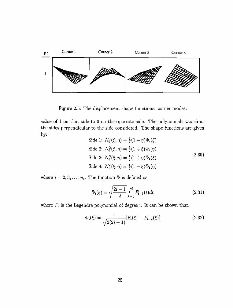
2.5 The displacement shape functions: corner modes ........................................... 25

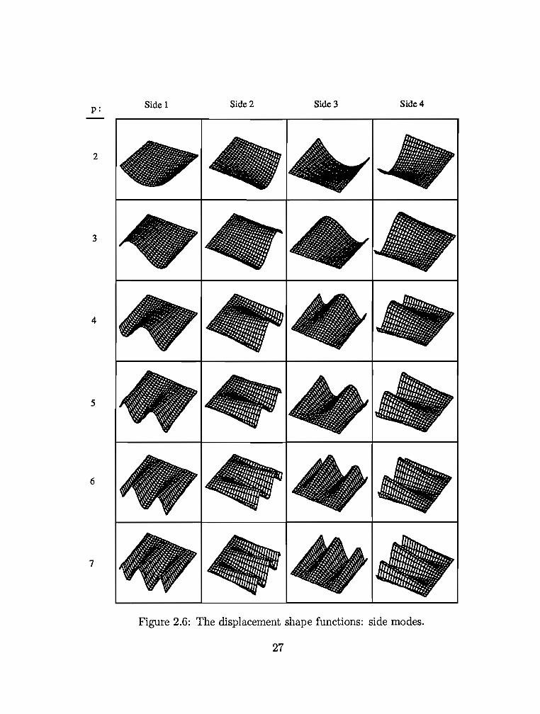
2.6 The displacement shape functions: side modes .................................... : ......... 27

2. 7 The displacement shape functions: internal modes ......................................... 29

2.8 Spanning set for polynomial shape functions .................................................... 30

2.9 Example of constraint count.. ............................................................................ 31

3.1 A bearing pad with surrounding obstacles ........................................................ 33

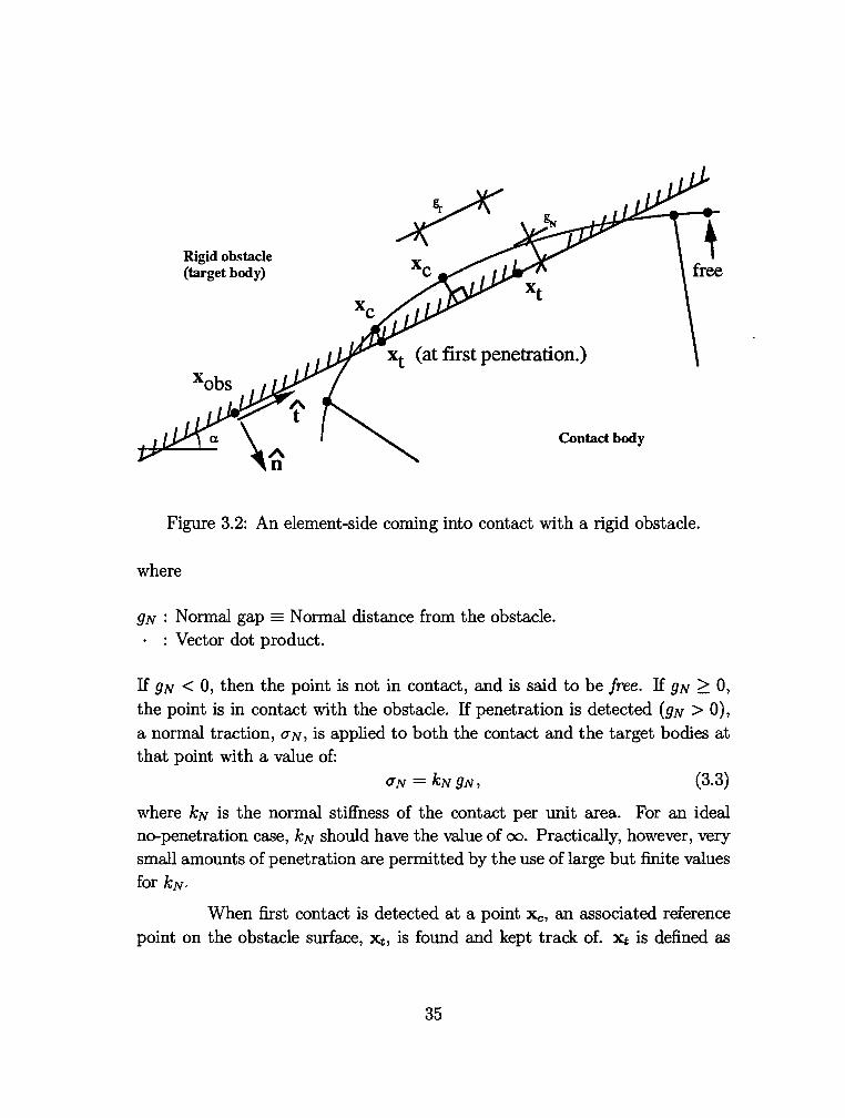
3.2 An element-side coming into contact with a rigid obstacle ................................ 35

3.3 The friction law .................................................................................................. 37

4.1 Glues, compressed piece of rubber analyzed using the 9-node element: Cases A and 8 .................................................................................................. 45

4.2 Glued, compressed piece of rubber analyzed using the 9-node element: Cases C and D .................................................................................................. 46

4.3 Glued, compressed piece of rubber analyzed using the higher-order element: Cases E, F and G .............................................................................. 4 7

4.4 Glued, compressed and sheared piece of rubber analyzed using: a) 20 nine-node elements; b) one higher-order element ........................................... 48

XI

4.5 The compression problem analyzed using one higher-order element with different constraint counts ................................................................................. 49

4.6 The compression-and-shear problem analyzed using one higher-order element with different constraint counts ............................................................ 50

4. 7 The compression-and-shear problem analyzed using one higher-order element with different integration rules ............................................................. 52

4.8 The meshes used for flat pads: a) 3 laminates; b) 6 laminates ....................... 53

4.9 Stress-strain relationship used for steel ............................................................ 55

4.10 Rubber contour plots for a compressed, 3-shim flat pad. cravg = -3447 KPa (-500 psi), G = 689.5 KPa (100 psi) ..................................................................... 57

4.11 Rubber contour plots for a compressed, 4% tapered pad, with 3 radial shims. cravg = -3447 KPa (-500 psi), G = 689.5 KPa (100 psi) ........................... 58

4.12 Deformed shapes for a 3-shim flat pad: a) under compression; b) compression and 50% shear. cravg = -3447 KPa (-500 psi), G = 689.5 KPa (100 psi) ............................................................................................................ 59

4.13 Deformed shapes for a 6-shim flat pad: a) under compression; b) compression and 50% shear. cravg = -3447 KPa (-500 psi), G = 689.5 KPa (100 psi) ............................................................................................................ 60

4.14 Rubber contour plots for a compressed and sheared, 3-shim flat pad. cravg = -3447 KPa (-500 psi), G = 689.5 KPa (100 psi) ................................................ 61

4.15 Pressure distribution at top of a flat pad under compression. cravg = -3447 KPa (-500 psi), G = 689.5 KPa (100 psi) .......................................................... 62

4.16 Contour plot for effective stress in the steel of a 3-shim 'flat pad under compression: cravg = -3447 KPa (-500 psi); cryield = 275.8 MPa (40E + 03 psi); contour values creffl'cryeidl: a} 0.025, b) 0.0625, and c) 0.1 ................................. 64

4.17 Contour plot for effective stress in the steel of a 3-shim flat pad under compression and 50% shear: O"avg = -3447 KPa (-500 psi); cryield = 275.8 MPa (40E + 03 psi); contour values crefffcryield: a) 0.15, b) 0.275, and c) 0.4 .... 65

4.18 cr11 distribution in the steel along laminate interfaces in a 3-shim flat pad, under pure compression, and compression and 50% shear. cravg = -3447 KPa (-500 psi) ................................................................................................... 66

4.19 The meshes used for tapered pads: a) horizontal laminates; b) radial laminates. Slope = 4°/o ..................................................................................... 67

4.20 A static model for FXO in tapered pads with radial shims .................................. 68

XII

4.21 Compressive force vs. vertical displacement for a 3-shim flat pad (a one-inch strip) .............................................................................................................. 70

4.22 Deformed shape for a compressed 5-shim pad with a mismatch: slope of pad = 0%, slope of girder= 2% ......................................................................... 7 4

4.23 A block of rubber under simple shear ................................................................ 76

4.24 Shear stress vs. shear strain in simple shear .................................................... 77

4.25 Deformed shape for a plain glued flat pad under 1 00% shear .......................... 78

4.26 Shear force vs. horizontal displacement for a 3-shim flat pad (a one-inch strip). cravg = -3447 KPa (-500 psi), G = 689.5 KPa (100 psi) ............................ 80

4.27 Change in vertical displacement upon shearing the pad ................................... 81

4.28 Stress-strain curve from simple shear test used to fit material constants .......... 85

4.29 The mesh used for the 2-shim flat pads ............................................................ 86

4.30 Deformed shape for a 2-shim flat pad under compression and 50% shear. cravg = -4378 KPa (-635 psi) .............................................................................. 86

4.31 Analytical vs. experimental shear force-deflection curves for a 2-shim flat pad (a one-inch strip): a) Gn = 689.5 KPa; b) Gn = 1379 KPa ......................... 87

5.1 The complex modulus ....................................................................................... 90

5.2 Illustration of the relationship between relative velocity and the hysteresis component of friction ......................................................................................... 93

5.3 Fhys as a function of vr ...................................................................................... 94

5.4 Sharp vs. round asperities ................................................................................ 95

5.5 Effect of temperature on friction of rubber ......................................................... 96

5.6 Effect of temperature and lubricant type ........................................................... 96

5. 7 Voigt model ....................................................................................................... 98

5.8 Cone-shaped asperities .................................................................................... 99

5.9 The interface and the friction law .................................................................... 101

5.10 Girder, pad and abutment nodes and the forces acting on them .................... 104

5.11 Cross-section of pad at Slaughter Creek bridge .............................................. 109

XIII

5.12 Time needed for a pad to slip a specified distance vs. slope .......................... 111

5.13 The distance the pad slips in 30 days as a function of E ...........•...........•.......•• 111

5.14 The motion of the top and the bottom of the pad and the girder in the case: slope= 0, E = 10-8

••••••••••••••..•.••••.••••.••••.••••••••.••••••..•.••••••.•••.••••••••...•.•.••••..••••••• 113

5.15 The motion of the top and the bottom of the pad and the girder in the case: slope= 0, E = 10-3

............•...•....•.............................•.............•..........•••••.•...•..•. 114

5.16 The motion of the to and the bottom of the pad and the girder in the case: slope= 1°/o, E = 10-8

••••.••.••••..•••••••••••..•••••••••••••••••••.••••••••••••••.•••••.•..•••••••••••••••.• 115

5.17 The motion of the top and the bottom of the pad and the girder in the case: slope= 1°/o, E = 5 X 10-5

..............••.....................•••........•...............•.•............•.• 116

5.18 The motion of the top and the bottom of the pad and the girder in the case: slope= 1°/o, E = 2 X 10-4

...............•.................................................................. 117

5.19 The motion of the top and the bottom of a tapered pad and the girder in the case: FX = Ksheari0<. > ,...FY, E = 10-8

••.•••••...•••.....••••.••••••••••••••.••.••••••••••.••••..••.• 119

5.20 The motion of the top and the bottom of a tapered pad and the girder under the vertical load of the girder only: a) E = 10-3

, b) E = 10-6 •...•...........•..•......••.. 120

XIV

SUMMARY

A two-dimensional nonlinear p-version finite element method is developed for the analysis of boundary value problems relevant to elastomeric bridge bearings. The method incorporates polynomial shape functions of the hierarchic type for the modeling of large­deformations rubber elasticity. In addition, a frictional-contact algorithm based on a penalty formulation and suitable for the interaction of the pad with rigid flat surfaces is derived and implemented. The J2-flow theory with isotropic hardening is utilized to model the reinforcing steel as a bilinear elastoplastic material. Examples are presented to illustrate the performance of the element and some guidelines for the selection of appropriate orders of interpolation and integration rules. The results of a study performed to examine the effects of several design parameters of the bearing are presented. Comparisons with experimental findings are shown.

A dynamic lumped model for the walking of the bearing is developed. Viscous frictional interfaces with the girder and the abutment are included. Several cases are analyzed to investigate the factors which affect this phenomenon.

XV

Chapter 1

INTRODUCTION

1.1 Elastomeric Bearings

Advances in structural analysis and design, in addition to the devel­opment of high-strength materials and new construction techniques, have made possible large structures with long spans. Due to various causes, large struc­tural components may experience substantial movements. These movements can be accommodated by either designing the structure and its foundations to absorb the forces which develop, or by separating the neighboring components by bearings. The bearings can be designed to transfer only some forces and to prevent the transfer of others.

In bridges, the superstructure moves due to temperature effects, mov­ing loads, earthquakes, concrete shrinkage and creep, etc. Unless bearings are used to accommodate the effects of these movements, the girders will apply large horizontal forces on the piers. Several types of bearing pads have been used to support the girders on the abutment: sliding devices, rolling devices, rockers, and elastomeric bearings [1].

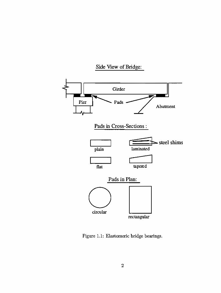
In plan, elastomeric bearings are circular or rectangular. In cross­section, they are either flat or tapered to accommodate an inclined girder in a bridge with slope (Figure 1.1). Moreover, the pads can be either plain or laminated (Figure 1.1). Plain bearings are made up of a layer of rubber which is thin relative to its in-plan dimensions. These bearings are appropriate only for bridges with small loads and short spans. For long spans, however, thicker pads are needed to absorb the large shear deformations. Thick layers of rubber do not have enough stiffness to carry the high compressive loads without excessive distortion and bulging of the sides. The shape factor (S), defined as the ratio of the loaded area to the area on the sides free to bulge, is a measure of the bulging restraint. It can be shown [2, 3, 4, 5] that the compressive stiffness of a block

1

Side View of Bridge:

Girder

Pads in Cross-Sections :

plain

flat

~steel shims laminated

J tapered

Pads in Plan:

0 circular

rectangular

Figure 1.1: Elastomeric bridge bearings.

2

made of an incompressible rubber is roughly proportional to S2. Therefore, in order to increase the compressive stiffness (Kcornp) of the pad, S has to be increased. In most cases, this is done by reinforcing the pads with laminates of steel placed in planes perpendicular to the compressive load direction, so as to divide the rubber into thinner layers. This significantly increases Kcarnp while preserving the shear flexibility. The pad in this case is said to be laminated. In a few cases, the bearing is reinforced with fibers; the present work, however, is concerned with steel-reinforced bearings.

One of the first uses of rubber pads was in Australia, in the year 1889 [6]. Plain natural rubber pads were used to support a viaduct on top of the piers. The pads are still functioning well; degradation is only within one millimeter of the surface. The first major application of laminated natural rubber bearings was in Pelham Bridge, Lincoln (UK). The pads were installed in 1955, and the bridge was opened in June 1958 (7].

In the United States, Texas, California, Florida, North Dakota, and Rhode Island were the first states to use elastomeric pads in bridges in the 1950's [8]. At the same time, Great Britain and France were using them in railroad bridges. Elastomeric bearings are also used in other structural appli­cations [9, 10, 6]: antivibration mountings for railroads and buildings, pads in precast parking structures, and base-isolation devices for structures in earth­quake zones.

Elastomeric bearings are the most widely used bridge-support systems because they [8, 11, 12]:

• are effective. While having high compressive stiffness, they are flexible enough in shear to prevent the transfer of harmful shear forces to the abutment. In addition, they immediately start to deform in shear; i.e., there is no static friction to overcome as in the case of sliding devices.

• do not have any moving parts which may freeze.

• distribute the load evenly and absorb vibrations.

• are simple.

• are easy to install.

3

• are compact.

• are weather-resistant.

• have low initial and installation costs.

• require little or no maintenance.

Rubber is defined as [7]: "Any material which can undergo large de­formations and recover almost completely and instantaneously on the release of the deforming forces." This kind of material was originally obtained from the tree Hevea Brasiliensis and called rubber or India rubber due to its pencil-lead erasing properties. It is also called Caouchouc which comes from the Indian word Caa-o-chu or the weeping tree. Rubber is a material which belongs to a broader group called polymers. A polymer is a material with long chain molecules made up of repeated small units (mers). IT these molecules are long and chemically joined at only few points (cross links), over a range of tempera­tures, they will have the elastic property of the rubber. Hence, they are called elastomers.

Two different types of rubber are used in elastomeric bearing pads: Natural Rubber (NR) and Synthetic Rubber (SR) [1]. During and after World War II, due to high demand for rubber as well as the restrictions on natural rub­ber supplies, synthetic rubbers were developed and before long came into wide spread use. That included their application in elastomeric bearings. The syn­thetic rubbers most used in bridge bearings are: Neoprene (polychloroprene), Butyl (polyisobutylene), and Nitrile (butadiene-acrylonitrile).

Natural rubber, when slightly stretched, loses most of its resistance to cracking by ozone. Therefore, special waxes are mixed with it, which migrate to the surface and form a protective coating. Neoprene and Butyl, on the other hand, have inherent ozone-resistance. Some countries (e.g., Germany) prohibit completely the use of natural rubber in elastomeric bridge bearings [13].

Manufacturing of rubber starts with the raw polymer, which is either natural or synthetic [14, 15, 1, 16, 6]. In the original form, the molecules of these materials are not linked together. Other substances are added to the raw polymer: vulcanizing agents (usually sulphur); reinforcing fillers (usually

4

carbon black); and other ingredients, such as antioxidants, antiozonants (wax), mixing oil and vulcanization accelerators. These materials are then blended to give a homogeneous mix. Layers of this mix and laminates of steel are put together in a mold which has the required shape of the pad. They are heated to about 140° C under pressure for a period of time, so that the vulcaniza­tion (cross-linking) process can take place. The rubber is then referred to as vulcanized rubber.

1.2 State of the Art

1.2.1 Methods of Analysis

Methods of the structural analysis of elastomeric bearings can be classified as either approximate analytical or rigorous discrete methods. In the approximate methods, simplifying assumptions about the material behavior, stress field and the deformed shape are introduced in order to produce ana­lytical solutions (deformed shapes, stresses, stiffnesses) of the pad idealized as a block of rubber. The solution may incorporate empirical factors which are calibrated experimentally. It is only possible to solve for very simple and usu­ally idealized deformations by these methods. Some of the first researchers to investigate such problems were: A.N. Gent, P.B. Lindley, E.A. Meinecke, F. Conversy, and B.P. Holownia. The stiffness relations developed were utilized in many specifications as the basis for bearing design. For examples of these and other similar approaches, see [2, 3, 17, 18, 19, 6, 20, 21, 22, 11, 23, 24, 4, 5, 25].

In order to analyze the pad in a more rigorous way, numerical methods can be used to solve the field equations. To this end, several approaches have been exploited. Soni and Becker [26] developed a method in which the pad is assumed to consist of a linear elastic material. This material is the result of smearing a heterogeneous continuum into an equivalent homogeneous one. The finite element method was used to solve the resulting equations. Holownia [20], assuming a linear elastic material and small deformations and strains, solved the problem using the finite difference method. Herrmann and co-workers [27, 28], employing the idea of an equivalent homogeneous continuum, performed a nonlinear (material and geometry) finite element analysis of the pad. They refer to their analysis as a 'composite analysis.'

5

The general finite-element-based method of analysis deals with the medium as an inhomogeneous continuum. The steel laminates are modeled as an elastoplastic material, and the rubber layers as a nonlinear elastic (hypere­lastic) incompressible (or nearly incompressible) material. Large deformations are taken into account. Most finite element analyses of elastomers use the quadratic isoparametric (Lagrangian) element [29, 30, 31, 32, 33, 34, 35, 36, 37, 38].

The incompressibility condition of the rubber is enforced by either the penalty method or the Lagrange multiplier method. In the penalty method, the displacements are the only unknown field variables to be interpolated and solved for. On the other hand, in the Lagrange multiplier method, both the displacements and the pressure have to be interpolated. The incompressibil­ity condition, which is introduced as a mathematical idealization to simplify the problem, is satisfied approximately in the penalty method and exactly in the Lagrange multiplier method. Under high hydrostatic pressures, how­ever, the slight compressibility becomes an important factor to consider in the analysis. The rubber, hence, can be modeled as a nearly incompressible (quasi­incompressible) material. A dilatation-like unknown can then be introduced as an additional field variable, interpolated over the domain, and solved for.

In the analysis, contact between elastomeric bearings and neighboring bodies can be dealt with in two ways: approximately or rigorously. In the first way, complete attachment is assumed to exist between the two contacting bodies. Therefore, the phenomena of frictional slip, lift, and roll-over of edges can not be captured (Figure 1.2). In more rigorous approaches, a frictionless or frictional-contact algorithm is used for more realistic modeling.

1.2.2 Finite Element Adaptive Methods: the p-version

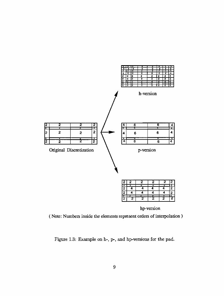
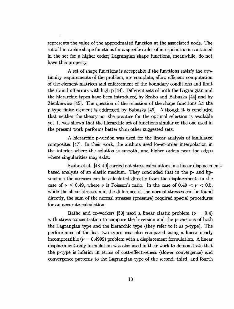
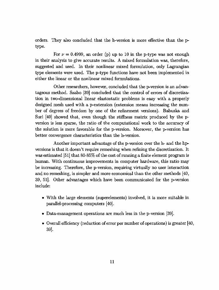
Since the earliest applications of the finite element method to complex and nonlinear problems, the question of the reliability of the solutions and ways to improve them became essential. Methods have been developed to estimate the errors in the solution and to try to control them. As illustrated in Figure 1.3, a finite element discretization can be refined using any of the following three versions [39, 40]:

6

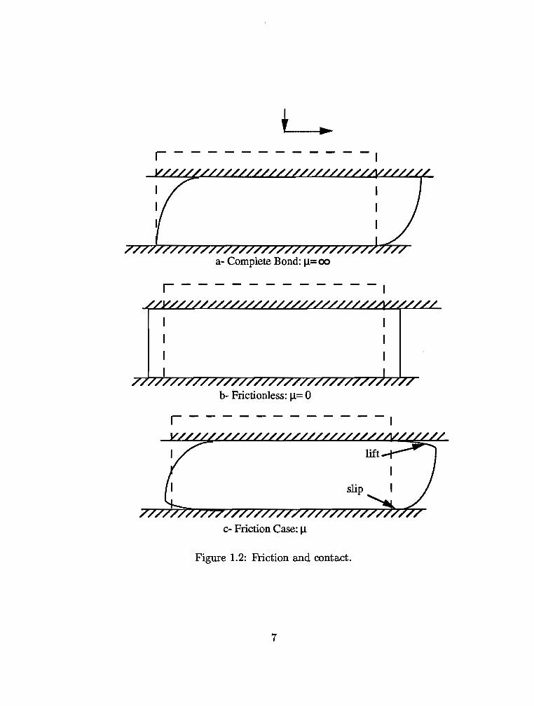
r------ -I

a- Complete Bond: 1.1= oo

r -I

b- Frictionless: 1.1= 0

r --,

c- Friction Case: ll

Figure 1.2: Friction and contact.

7

• h-version: In this version, the mesh is enriched with smaller elements of the same order. his a norm for measuring the element size.

• p-version: In this version, the errors are controlled by increasing p, the order of the approximating functions.

• hp-version: This version is a hybrid of the first two. The element sizes, h, are decreased and the order of the interpolating functions, p, are si­multaneously increased.

Another method, referred to as the Fast Adaptive Composite Grid Method [41], has been used to improve the finite element solutions. This method uses iterations between a global coarse mesh and local refined meshes (over areas of high errors) in order to drive the coarse-fine interface residuals to zero.

Methods for improving the domain discretization are also called adap­tive methods. A finite element method is called self-adaptive when it is asso­ciated with an error estimate and the mesh is refined (adapted) automatically if needed.

The h-version has essentially been used since the advent of the finite element method. Furthermore, the idea of using higher-order approximating functions in numerical methods has been known and used for a long time. It was not, however, until early in the 1970's that the p- and hp-versions began to be investigated and applied in a finite element context by Szabo [40].

. The first paper to appear on the p-version was [42] and on the hp­version was [43]. Since then much research has been done on implementing these methods into a broad range of finite element applications: plane elastic­ity, plates and shells, stability, fracture mechanics, fluid mechanics, nonlinear elasticity, and transient problems. For an extended bibliography, see [40].

The shape functions used in conjunction with a p-version can be either Lagrangian or hierarchic. A Lagrangian shape function is associated with a specific node in the element; its value equals one at that node and zero at the remaining nodes. A hierarchic mode, on the other hand, doesn't have to satisfy this property. While the coefficient associated with a hierarchic mode doesn't necessarily have a physical meaning, a Lagrangian degree of freedom

8

2 2 2 2 2 2 2

2 2 12 2 2 2 2 2 2 2 2 2 2 2 2 2 2 2 2 2 2 2 2

2 2 2 2 2 2 2 2

h-version

2 2 2 2 4 6 6 4

., ? 2 2 4 6 6 4

2 2 ' 2 4 6 6 4

Original Discretization p-version

2 2 2 2 2 2

2 4 4 4 4 2 2 4 4 4 4 2

2 2 2 2 2 ' hp-version

(Note: Numbers inside the elements represent orders of intetpolation)

Figure 1.3: Example on h-, p-, and hp-versions for the pad.

9

represents the value of the approximated function at the associated node. The set of hierarchic shape functions for a specific order of interpolation is contained in the set for a higher order; Lagrangian shape functions, meanwhile, do not have this property.

A set of shape functions is acceptable if the functions satisfy the con­tinuity requirements of the problem, are complete, allow efficient computation of the element matrices and enforcement of the boundary conditions and limit the round-off errors with high p (44]. Different sets of both the Lagrangian and the hierarchic types have been introduced by Szabo and Babuska [44] and by Zienkiewicz (45]. The question of the selection of the shape functions for the p-type finite element is addressed by Babuska [46]. Although it is concluded that neither the theory nor the practice for the optimal selection is available yet, it was shown that the hierarchic set of functions similar to the one used in the present work performs better than other suggested sets.

A hierarchic p-version was used for the linear analysis of laminated composites [47]. In their work, the authors used lower-order interpolation in the interior where the solution is smooth, and higher orders near the edges where singularities may exist.

Szabo et al. [48, 49] carried out stress calculations in a linear displacement­based analysis of an elastic medium. They concluded that in the p- and hp­versions the stresses can be calculated directly from the displacements in the case of v < 0.49, where v is Poisson's ratio. In the case of 0.49 < v < 0.5, while the shear stresses and the difference of the normal stresses can be found directly, the sum of the normal stresses (pressure) required special procedures for an accurate calculation.

Bathe and co-workers [50] used a linear elastic problem (v = 0.4) with stress concentration to compare the h-version and the p-versions of both the Lagrangian type and the hierarchic type (they refer to it asp-type). The performance of the last two types was also compared using a linear nearly incompressible (v = 0.4999) problem with a displacement formulation. A linear displacement-only formulation was also used in their work to demonstrate that the p-type is inferior in terms of cost-effectiveness (slower convergence) and convergence patterns to the Lagrangian type of the second, third, and fourth

10

orders. They also concluded that the h-version is more effective than the p­type.

For v = 0.4999, an order (p) up to 10 in the p-type was not enough in their analysis to give accurate results. A mixed formulation was, therefore, suggested and used. In their nonlinear mixed formulation, only Lagrangian type elements were used. The p-type functions have not been implemented in either the linear or the nonlinear mixed formulations.

Other researchers, however, concluded that the p-version is an advan­tageous method. Szabo [39] concluded that the control of errors of discretiza­tion in two-dimensional linear elastostatic problems is easy with a properly designed mesh used with a p-extension (extension means increasing the num­ber of degrees of freedom by one of the refinement versions). Babuska and Suri (40] showed that, even though the stiffness matrix produced by the p­version is less sparse, the ratio of the computational work to the accuracy of the solution is more favorable for the p-version. Moreover, the p-version has better convergence characteristics than the h-version.

Another important advantage of the p-version over the h- and the hp­versions is that it doesn't require remeshing when refining the discretization. It was estimated [51] that 80-85% of the cost of running a finite element program is human. With continuous improvements in computer hardware, this ratio may be increasing. Therefore, the p-version, requiring virtually no user interaction and no remeshing, is simpler and more economical than the other methods [40, 39, 51]. Other advantages which have been communicated for the p-version include:

• With the large elements (superelements) involved, it is more suitable in parallel-processing computers [40].

• Data-management operations are much less in the p-version [39].

• Overall efficiency (reduction of error per number of operations) is greater [40, 39].

11

1.2.3 Contact Algorithms

Contact algorithms are designed to model the interaction of two bod­ies at the surface where they are touching each other. Physically, no penetration of one body into the other takes place, and in the shear direction, friction forces develop to resist one body's attempt to translate tangent to the other. The contact also involves plastic deformations, plowing and wear of the contacting bodies.

Early solutions for the contact problem were based on the classical elasticity theory [52, 53]. With the use of numerical methods to solve solid mechanics problems, new contact algorithms were developed. Those methods varied in their complexity, ranging from complete bond to the cases of friction­less and frictional contact and slip {Figure 1.2).

Different approaches are used to enforce the boundary conditions as­sociated with contact: the penalty method [54, 31, 55], Lagrange multiplier method [56, 57, 58, 59, 60] and hybrid or mixed methods [52]. Solution tech­niques can be explicit or implicit [54, 61]. In the penalty formulation, normal and tangential springs are introduced at the contact surface. No additional unknowns are involved in this method. In a mixed formulation, however, both the displacements and the tractions at the surface are included in the set of unknowns of the problem, and are solved for directly.

The penalty method satisfies the contact condition of no penetration only approximately; the multiplier method, on the other hand, satisfies the condition exactly. However, while the multiplier method increases the sizes of the finite element matrices and the number of degrees of freedom, the penalty method keeps them intact. In addition, the stiffness matrix in the multiplier method is indefinite and has zero diagonal terms that may cause some prob­lems [60]. On the other hand, the accuracy of the penalty method is dependent on the choice of the penalty parameter.

Different friction laws have been suggested for use in contact algo­rithms [62]. The regularized Coulomb law is the most popular one. Other laws, based on plasticity theory, are represented mathematically by polyno­mial relationships between the shear and the normal tractions [63, 55, 56]. Coulomb's law represents a special case in which the polynomial order equals

12

one. In plasticity-based laws, the yield surface represents a sliding surface. These laws involve an elastic part followed by a plastic (sliding) part.

1.3 Objective

In the present work, a two-dimensional p-version finite element method for the analysis of the elastomeric bearings is presented. The method is based on a large-deformations and large-strains formulation. The steel is modeled as a bilinear elastoplastic material. The J2-flow theory with isotropic hardening is utilized. The rubber is considered an incompressible hyperelastic material, and the Lagrange multiplier method is used to enforce incompressibility.

The application of a p-version with functions of the hierarchic type is investigated for the boundary value problems relevant to the analysis of elastomeric bearings. The order of pressure interpolation required for a specific displacement interpolation order is discussed. Integration rules necessary with the higher-order functions are examined. In addition, a contact algorithm based on a penalty formulation is derived and implemented. It incorporates the regularized Coulomb friction law. The algorithm is appropriate for the contact of the large elements of the p-version with rigid flat surfaces which move as rigid bodies.

A study is performed to examine some parameters which affect the performance and the design of the pad. Some analyses are compared with experimental results. Examples are presented to illustrate some aspects of the higher-order element.

In Chapter five, a lumped dynamic model for the out-of-place trans­lation of the pad (walking) is developed. Viscous frictional interfaces with the girder and the abutment are included. Several cases are analyzed to examine the factors which affect this phenomenon.

13

Chapter 2

P-VERSION FINITE ELEMENT METHOD

2.1 Introduction

A p-version finite element method is used to model elastomeric bear­ings in a two-dimensional plane-strain setting. The elastomer is treated as an incompressible elastic material undergoing large deformations (a hypere­lastic material). The incompressibility condition in enforced by the Lagrange multiplier method where the multiplier is a pressure-like variable. Therefore, both the displacement and the pressure fields need to be interpolated over the domain of the problem. When steel, which is modeled as a bilinear elasto­plastic material, is used to reinforce the elastomer, only the displacements are interpolated over the laminates.

The higher-order shape functions used for displacement interpolation are of the hierarchic type. The functions used for pressure interpolation are, besides being hierarchic, nonconforming (i.e., discontinuous at element bound­aries). In this chapter, a brief introduction to large-deformation kinematics and to constitutive modeling of hyperelastic materials is given. Next, the boundary value problem is discretized. by the finite element method. Then, the higher­order functions are presented. Finally, aspects of interpolation orders and nu­merical integration are discussed.

2.2 Large-Deformation Kinematics

When a body undergoes large deformations, a clear distinction be­tween its position before and after deformation is drawn and a different set of kinematic quantities are defined. Assume that the body n deforms from the reference (usually the undeformed) configuration no to the current (deformed)

14

X

'dX Reference Configuration

X

Current Configuration

Figure 2.1: Mapping X from no to nc.

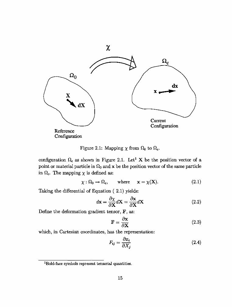
configuration nc as shown in Figure 2.1. Let1 X be the position vector of a point or material particle in no and x be the position vector of the same particle in flc. The mapping X is defined as:

where x = x(X). (2.1)

Taking the differential of Equation ( 2.1) yields:

ax ax dx axdX= axdX (2.2)

Define the deformation gradient tensor, F, as:

8x F=-

8X (2.3)

which, in Cartesian coordinates, has the representation:

(2.4)

1 Bold-face symbols represent tensorial quantities.

15

F maps infinitesimal vectors (dX.) from the reference configuration into infinitesimal vectors (dx) in the current configuration (FdX. = dx). It can be shown that the ratio of the volume of an infinitesimal element in Oc ( dv) to its volume in 0o (dV) equals the determinant ofF (also called the Jacobian determinant, J):

J=detF dv dV

(2.5)

Since the material occupying any volume in the original configuration must also occupy positive volume when deformed, J must always satisfy: J > 0.

The deformation gradient F can be decomposed (polar decomposition theorem) into two components:

F=RU (2.6)

where

R : An orthogonal tensor (i.e., RR T I = The Identity tensor; superscript T indicates the transpose).

U : A symmetric positive-definite tensor.

The decomposition ( 2.6) is unique. Moreover, component U acts first on the material of the body at point X (in flo) followed by R which does not distort the material any more but only applies a local rigid body rotation. Therefore, R, which is called the rotation tensor, does not produce any additional stresses. All stretching information is stored in U only, hence it is called the stretch tensor.

The principal directions of U are the solutions of:

(i=1,3)

where

u1 : ith principal direction of stretch (eigenvector· of U). ,\i : ith principal stretch (eigenvalue of U).

16

(2.7)

F=U

1.0

1.0

Undeformed Deformed

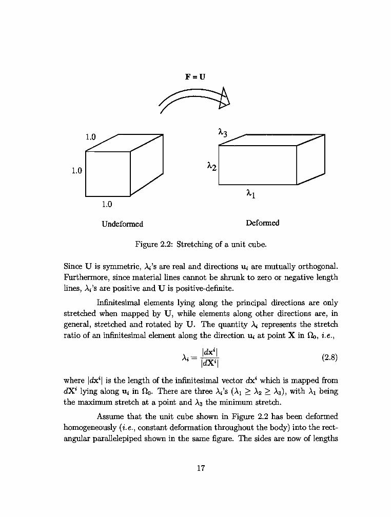
Figure 2.2: Stretching of a unit cube.

Since U is symmetric, ..\/s are real and directions 11i are mutually orthogonal. Furthermore, since material lines cannot be shrunk to zero or negative length lines, ..\/s are positive and U is positive-definite.

Infinitesimal elements lying along the principal directions are only stretched when mapped by U, while elements along other directions are, in general, stretched and rotated by U. The quantity ..\i represents the stretch ratio of an infinitesimal element along the direction Ui at point X in no, i.e.,

(2.8)

where ldxil is the length of the infinitesimal vector dxi which is mapped from dXi lying along ui in no. There are three ..\i's (..\1 ~ A2 > Aa), with AI being the maximum stretch at a point and ..\3 the minimum stretch.

Assume that the unit cube shown in Figure 2.2 has been deformed homogeneously (i.e., constant deformation throughout the body) into the rect­angular parallelepiped shown in the same figure. The sides are now of lengths

17

..\1 , ..\2 , and ,\3 and are parallel to their undeformed positions. The deformation gradient is given by:

F [

~01 ~2 0 ] 0 ~3

(2.9)

and the Jacobian determinant:

J _ d F _ dv _ ..\1,\2..\a _ , , , = et - dV - 1 - "'1"'2"'3 (2.10)

It is clear that for this case U F and R = I.

In order to remove the R component which does not contribute to the stresses, the right Cauchy-Green tensor is defined as:

(2.11)

While F is not necessarily symmetric, C is clearly symmetric and positive­definite. Define the principal invariants of C as :

f 1 traceC

f 2 ![(traceC)2- traceC2]

fa= detC

For the cube example introduced above, C is given by:

and

C=U2= [ ~Oi ~~ ~] 0 ,\~

h =.Ai+.A~+.A~ f2 = (,\1..\2)2 + (..\2..\a)2 + (.Aa..\1)2

fa (A1A2Aa)2 = F

If the material is incompressible, then:

J = ,\1,\2,\3 1

(2.12)

(2.13)

(2.14)

(2.15)

For more information on the kinematics of large deformations, one can refer to [64, 65].

18

2.3 Hyperelastic Incompressible Materials

Hyperelastic materials are characterized by a strain energy density function, E. For an isotropic hyperelastic material, E can be written as a function of the principal invariants of C:

(2.16)

In this study, the rubber is idealized as an incompressible material with the incompressibility condition enforced using the Lagrange multiplier method. Different choices could be used for the constraint equation and the associated multiplier; for example:

c= /3 -1 = 0 (2.17)

could be used. The multiplier in this case represents the hydrostatic pressure. For the incompressible case, the function E becomes:

(2.18)

For hyperelastic incompressible materials, the Cauchy stress tensor is given by [64, 32]:

where

p : Hydrostatic pressure. I : Identity tensor. B: Left Cauchy-Green tensor (B = FFT).

(2.19)

Note that the constitutive behavior of the material is expressed in the functions :~ and :R. The pressure, p, cannot be obtained from the de­formation and must be obtained from equilibrium equations. Different mod­els are available for the strain energy density function E. For more details, see [66, 64, 67].

19

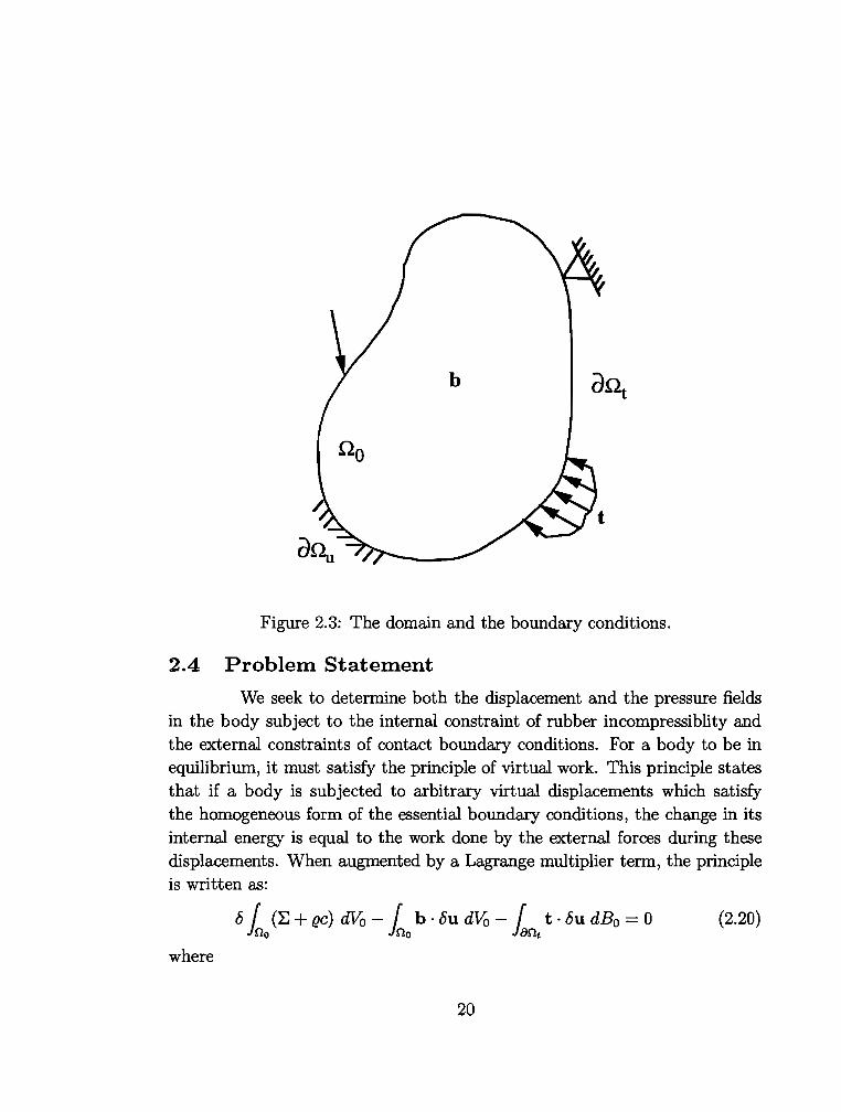
Figure 2.3: The domain and the boundary conditions.

2.4 Problem Statement

We seek to determine both the displacement and the pressure fields in the body subject to the internal constraint of rubber incompressiblity and the external constraints of contact boundary conditions. For a body to be in equilibrium, it must satisfy the principle of virtual work. This principle states that if a body is subjected to arbitrary virtual displacements which satisfy the homogeneous form of the essential boundary conditions, the change in its internal energy is equal to the work done by the external forces during these displacements. When augmented by a Lagrange multiplier term, the principle is written as:

6 f (E + gc) dVo - f b · 6u dVo - f t · 6u dB0 0 (2.20) lno lno lant

where

20

8 : The variational operator. no : The reference configuration of the domain. 8nt : Part of the boundary of the domain over which tractions are prescribed. E : Strain energy density function per unit volume. {} : Lagrange multiplier. c : For rubber: The incompressibility constraint equation; - 0, otherwise. u = x - X : Displacement vector field. x : Position vector in the current configuration. X : Position vector in the reference configuration. b : Body forces. t : Surface tractions. 8u : Virtual displacements. dVo : Infinitesimal volume element in the reference configuration. dB0 : Infinitesimal surface element in the reference configuration.

The last term in the above equation, representing the boundary con­ditions (contact forces in our case), is detailed in the next chapter.

2.5 Finite Element Discretization

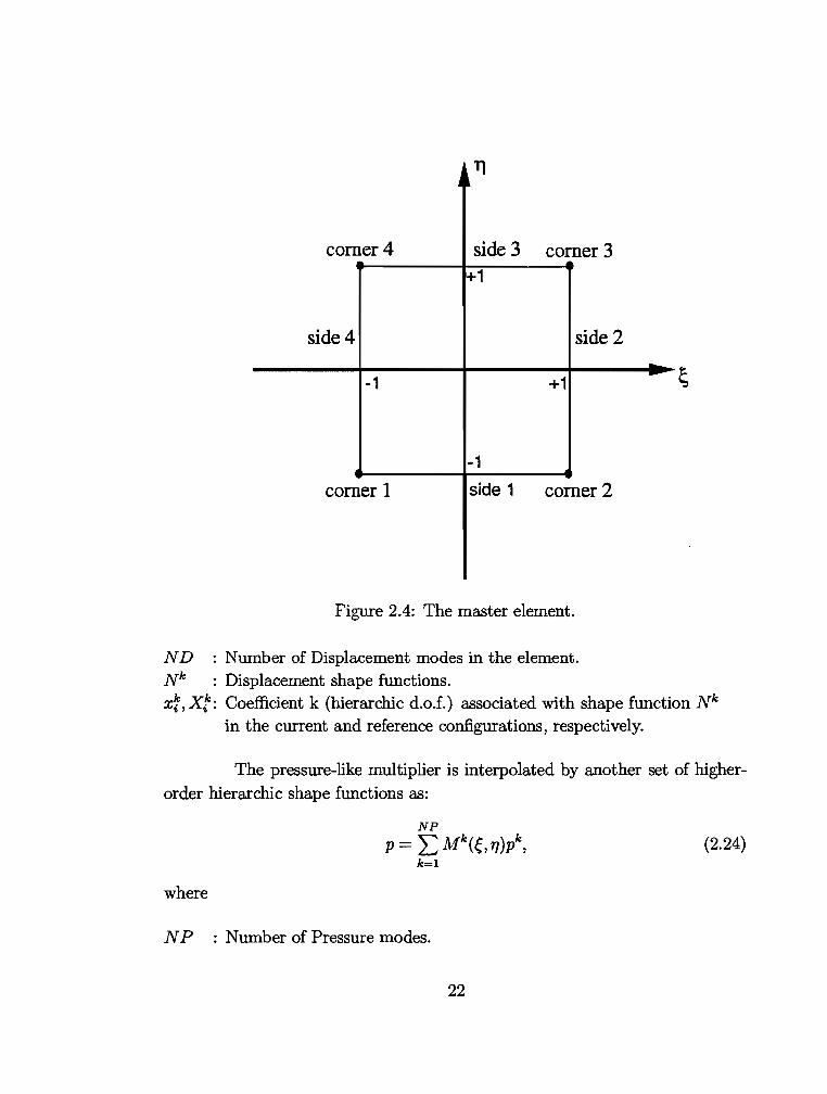
The domain is discretized into quadrilateral elements over which higher­order hierarchic shape functions are used to interpolate the displacements and the pressure. The elements are mapped from a master element (Figure 2.4) by an isoparametric map.

The ith_coordinate (i = 1, 2) of a point is interpolated as:

ND xi = L Nk(f., TJ)Xik reference configuration

k=l ND

Xi = L Nk (f., TJ )xf current configuration k=l

and the displacements:

ND

ui =xi- xi= I: Nk(t;., 17)(xf- x:), k=l

where

21

(2.21)

(2.22)

(2.23)

J~ 11

comer4 side 3 comer 3 +1

side4 side2 ... --1 +1

-1

comer 1 side 1 comer 2

Figure 2.4: The master element.

N D : Number of Displacement modes in the element. Nk : Displacement shape functions. xf,Xf: Coefficient k (hierarchic d.o.f.) associated with shape function Nk

in the current and reference configurations, respectively.

The pressure-like multiplier is interpolated by another set of higher­order hierarchic shape functions as:

NP p = 2: Mk(e,1])pk, (2.24)

k=l

where

NP : Number of Pressure modes.

22

Mk : Pressure shape functions. pk : Coefficient k associated with shape function Mk.

Using the chain ru1e, the variation in the strain energy density, 8E, can now be written as:

(2.25)

where summation over repeated indices is assumed. Similarly, the variation of the constraint term is given by:

(2.26)

with the pressure-like variable, p, representing Lagrange mu1tiplier, g.

Substituting the terms above into the virtual work statement (Equa­tion ( 2.20)) yields:

(2.27)

0

where

NUMEL: NUMber of ELements in the model. no : The domain of element e. 800 : Part of the element boundary where tractions are prescribed. bi, ti : ith-components of band t, respectively.

For arbitrary variations 8x~ and 8pk, a set of equations of the form:

(2.28)

is obtained, where I and F represent the internal and generalized nodal point forces, respectively. These equations represent a highly nonlinear set of equa­tions in the unknowns x and p which are solved incrementally using Newton's

23

method. Over each increment (step), several iterations are performed until the solution converges. The solution at each iteration represents displacement and pressure increments ( dx, dp) which are used to update these coefficients (x, p) from the previous iteration. Further details on the derivations and the individual terms can be found in [34].

2.6 Displacement Interpolation

Hierarchic shape functions of the type introduced by Szabo and Babuska (44, 46] have been used to map both the reference and the current configurations of the body from the master element. These shape functions are grouped int() three categories: corner modes, side modes and internal modes.

2.6.1 Corner Modes

This group is shown in Figure 2.5. Four bilinear shape functions with a value of one at the corresponding corner and zero along far sides are utilized:

(2.29)

where (e.h 1Ji) are the coordinates of corner i of the master element. All sub­sequent shape functions vanish at all four corners. Therefore, the coefficient associated with a corner shape function represents the value of the function being interpolated at that corner. If these shape functions only are used in an element, it will correspond to the familiar four-noded bilinear element.

2.6.2 Side Modes

There are Pi - 1 shape functions associated with side j, where Pi (> 2) is the order of interpolation along that side. In the present work, we have implemented the capability of having different orders (2 < Pi < 8) along different sides of each element as long as the same order is specified for the adjacent element sharing the same side to ensure continuity.

The side modes are given as products of polynomials in the direction of the side and a linear function in the perpendicular direction varying from a

24

p: Comer 1 Corner2 Comer 3 Comer4

1

Figure 2.5: The displacement shape functions: corner modes.

value of 1 on that side to 0 on the opposite side. The polynomials vanish at the sides perpendicular to the side considered. The shape functions are given by:

Side 1: Nl(f., 17) = t(l-17)4:>i(f.)

Side 2: N'f(f,, 17) t(l + f.)4:>i(17)

Side 3: Nl(f., 17) = !(1 17)4>i(f.)

Side 4: Nt(f.,17) = !(1- f,)4:>i(17)

where i = 2, 3, ... , Pi. The function 4:> is defined as:

where Fi is the Legendre polynomial of degree i. It can be shown that:

25

(2.30)

(2.31)

(2.32)

Functions q. i up to order 8 are given by the following formulas:

q,2(e) = e- 1

q,3(e) = e-e q,4(e) = se-4 - 6e2 + 1

q,s(e) = 7e5- we+~

q,6(e) = 21e6 - 3se4 + 1se2 - 1

q,7(e) = 33e - 63e5 + 35e - se

q,s (e) = 429e8 - 924e6 + 63oe - 14oe + 5

(2.33)

Functions in this group of order p < 7 are shown in Figure 2.6. All functions associated with side j up to order Pi are used (hierarchy). When Pi has a value less than two for a side, zero modes are contributed by that specific side. The coefficient associated with a side shape function of order two represents the deviation of the interpolated function from linear interpolation at mid-side. Geometric interpretation of higher-order coefficients is not straightforward.

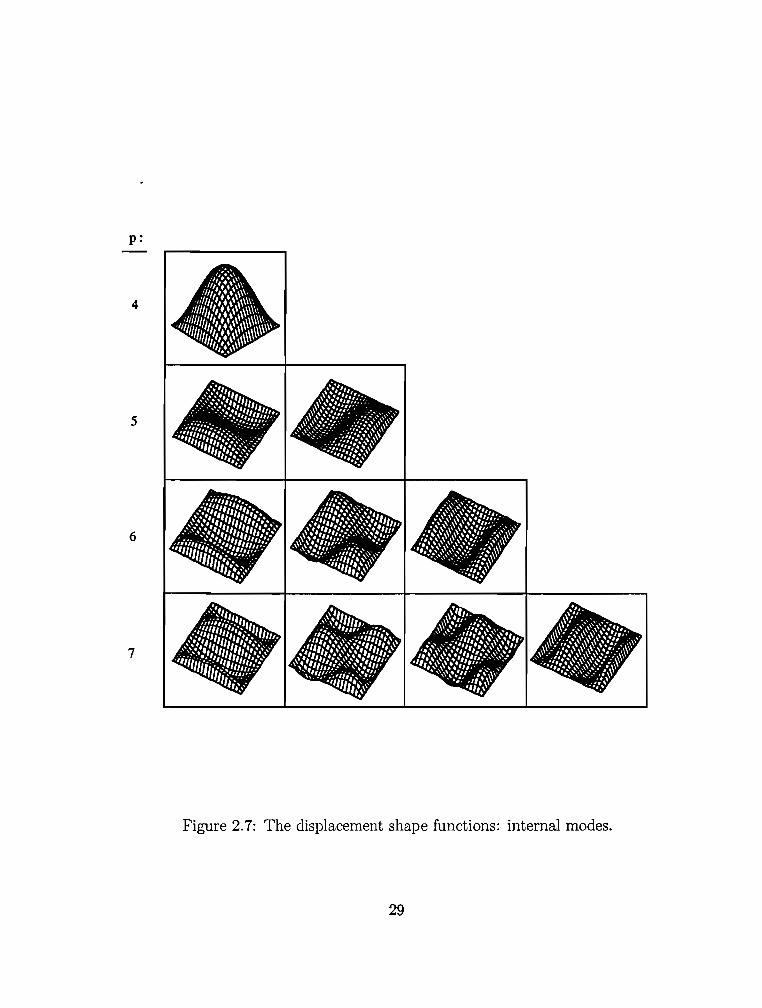
2.6.3 Internal Modes

Internal modes are given as products of polynomials in thee and TJ

directions. These shape functions vanish at all sides. There are NI = (p- 2)(p- 3)/2 modes, where (p > 4) is the interpolation order of the internal modes of the element at hand. p could be varied among elements and in general does not have to be the same as any of the sides of the element. Internal shape functions of order p are given by:

N1 = q,2(e)q,2(TJ)

N2 = q,2(e)q,3(T/)

N4 = q,2(e)q,4(TJ)

N3 = q,3(e)q,2(T/)

Ns = q,3(e)q,3(TJ) N6 q.4(e)q.2(TJ)

26

(2.34)

p:

2

3

4

5

6

7

Side 1 Side2 Side3 Side4

Figure 2.6: The displacement shape functions: side modes.

27

where the first N I modes are used. <Pi(e) is given by Equation ( 2.31) above. This group is shown in Figure 2.7 (pup to 7).

2. 7 Pressure Interpolation

The shape functions used here are of the non-conforming type. For order of interpolation equal top, the first N P = (p+ l)(p+2)/2 of the following polynomials are used:

M1=l

M2=e

M4=e

2.8 Order of Interpolations

(2.35)

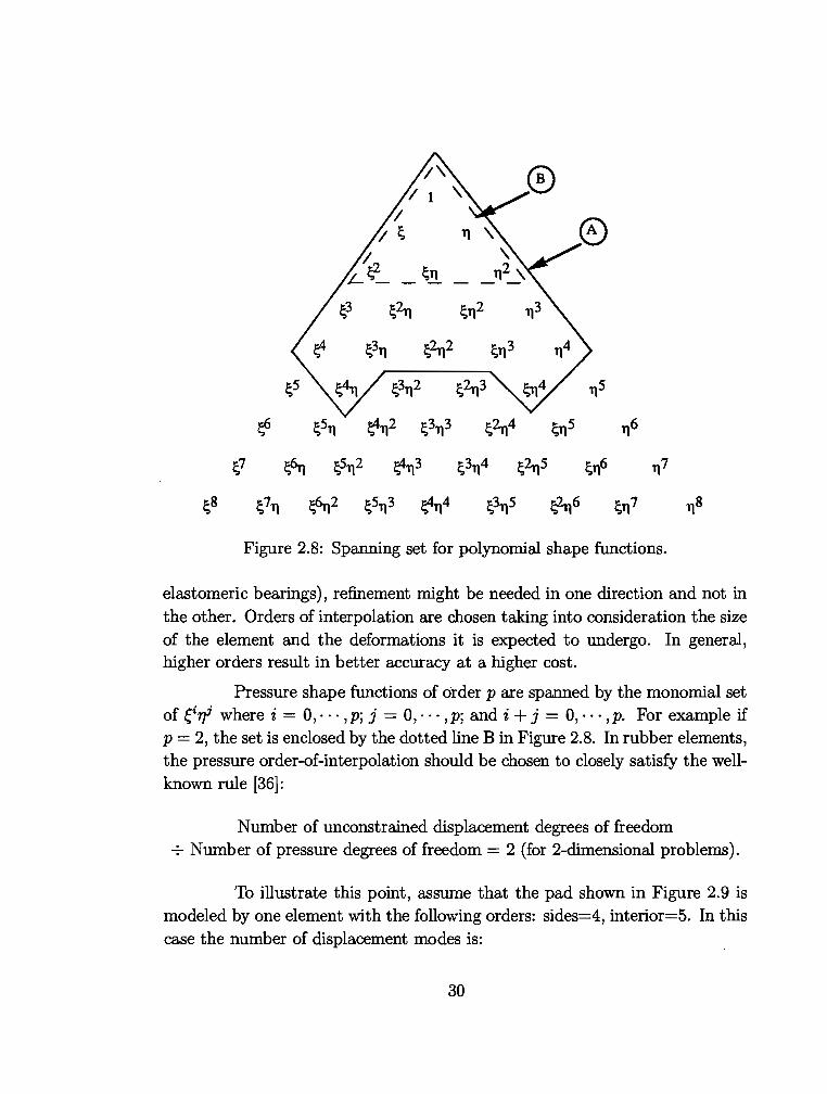
The polynomial shape functions presented above are linear combina­tions of monomials of the form eirf shown in Figure 2.8. For instance, let us assume that an order of four has been chosen for all the sides and the interior of an element. The spanning set of monomials for the shape functions in this case are grouped inside the solid line A in the same figure. This element has a displacement order of interpolation of four. H, however, any of the sides or the interior has an order less than four, some of the monomials of order < 4 may not be included and the order of interpolation would be less than four.

As mentioned earlier, p can be varied among elements as well as among the sides and the interior of each element. In order to guarantee a complete span of monomials up to order p over an element, that order should be specified for all the sides as well as the interior of that element. However, this rule can be violated in transition elements which lie between elements of different orders. In addition, as in the case of thin layered media (for example,

28

p:

4

5

6

7

Figure 2. 7: The displacement shape functions: internal modes.

29

s2rt s112

s311 s2rt2 s113

s3112 115

tf' s511 ~2 s3113 s2rt4 915 116

s1 ~ ss112 ~3 s3n4 s2rts srf' 117

ss s7n ~2 ss113 ~4 s3ns ;2rt6 sn7 118

Figure 2.8: Spanning set for polynomial shape functions.

elastomeric bearings), refinement might be needed in one direction and not in the other. Orders of interpolation are chosen taking into consideration the size of the element and the deformations it is expected to undergo. In general, higher orders result in better accuracy at a higher cost.

Pressure shape functions of order p are spanned by the monomial set of ~i'TJi where i = 0, · · · ,p; j = 0, · · · ,p; and i + j = 0, · · · ,p. For example if p = 2, the set is enclosed by the dotted line B in Figure 2.8. In rubber elements, the pressure order-of-interpolation should be chosen to closely satisfy the well­known rule [36]:

Number of unconstrained displacement degrees of freedom +Number of pressure degrees of freedom= 2 (for 2-dimensional problems).

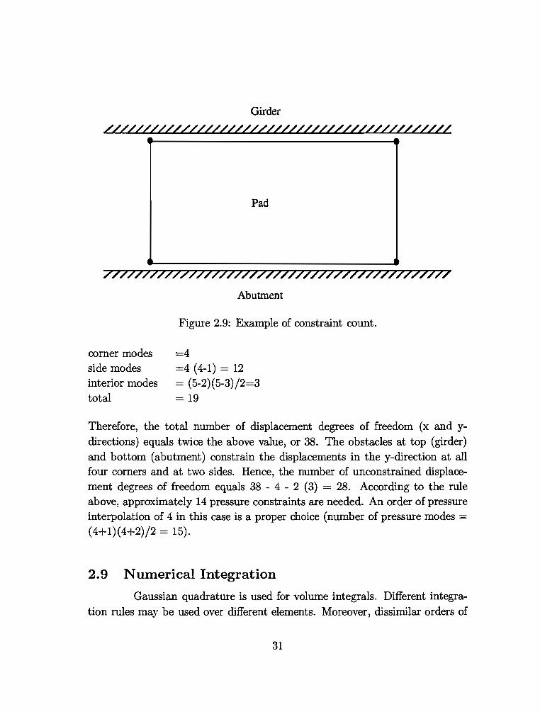
To illustrate this point, assume that the pad shown in Figure 2.9 is modeled by one element with the following orders: sides=4, interior=5. In this case the number of displacement modes is:

30

Girder

LL/LL///LL///////L//L////L/L//L////////LL/L/L

Pad

777777777777777777777777777777777777777777777

Abutment

corner modes side modes interior modes total

Figure 2.9: Example of constraint count.

=4 =4 (4-1) = 12 = (5-2)(5-3)/2=3 = 19

Therefore, the total number of displacement degrees of freedom (x and y­directions) equals twice the above value, or 38. The obstacles at top (girder) and bottom (abutment) constrain the displacements in they-direction at all four corners and at two sides. Hence, the number of unconstrained displace­ment degrees of freedom equals 38 - 4 - 2 (3) = 28. According to the rule above, approximately 14 pressure constraints are needed. An order of pressure interpolation of 4 in this case is a proper choice (number of pressure modes= (4+1)(4+2)/2 = 15).

2.9 Numerical Integration

Gaussian quadrature is used for volume integrals. Different integra­tion rules may be used over different elements. Moreover, dissimilar orders of

31

integration can be used in the e-direction and the 1]-direction over each element. The order of interpolation as well as the size of an element are important factors in selecting integration rules for that element. It has been observed that the integration rule should have an order at least equal to the order of displacement interpolation of the specific element. Higher orders of integration, however, re­sult in better deformed shapes towards the edges and in better enforcement of the incompressibility condition as illustrated by examples in Chapter 4. Surface integration is discussed in the next chapter.

32

Chapter 3

FRlCTIONAL-CONTACT ALGORITHM

3.1 Introduction

Bridge bearing pads come into contact at the bottom and the top (and possibly the sides under excessive shearing) with the rigid and plane surfaces of the abutment and the girder, respectively (Figure 3.1). These rigid surfaces are referred to here as obstacles. The contact is of a frictional type, and a stick-slip model is used. In the finite element model of the pad, all external

Girder 1 «UIIL tl/tlltll/ltttti/Lt/10{ .

Pad

777777777777777777777777777777777777777777777

Abutment

Figure 3.1: A bearing pad with surrounding obstacles.

element sides that may come into contact with an obstacle should be labeled in advance. During the analysis, these sides are checked for possible contact; appropriate contributions are added if contact is detected.

33

In this chapter, contact tractions are computed using a penalty for­mulation. The contribution of these tractions to the virtual work is then found, integrated over the contact surface, and differentiated for the incremental pro­cedure. Afterwards, the contact contributions to the finite element equations are derived. Finally, some practical considerations which aid the numerical method are discussed.

3.2 Frictional Contact at a Point by Penalty Formula­tion

In two-dimensional problems, the position of each obstacle is fully described by three degrees of freedom: two translations and a rotation. In the current application (bridge bearings}, the horizontal translations and the rotations are prescribed functions of time for both obstacles. In the vertical direction, the abutment's motion (zero displacement} and the girder's vertical load are usually prescribed. However, for generality, one degree of freedom, for which loads can be prescribed, is added to the set of unknowns for each obstacle representing its vertical displacement. This obstacle degree of freedom might be prescribed as in the case of the abutment. The position vector (Xobs = {Uobs V008 }T} of a point on the obstacle's surface and the angle (a} that the obstacle makes with the horizon (Figure 3.2} are used to describe the rigid body motion. The discretized model of the pad is referred to as the contact body and the rigid obstacle as the target body. The normal and tangent unit vectors, ii and t respectively, on the target-body surface are given by:

ii ={sin a - cosa}T t {cos a sina}T, (3.1}

where a = a(t).

Consider a point 1 Xc on an element-side along the boundary of the contact body and coming into contact with the target body. The gap, or the normal distance of the point Xc from the obstacle surface, is calculated as:

9N = -(Xc- Xobs} · ii, (3.2)

1 In the following, a point p may be referred to by its pa.ition vector in the current configuration, x.

34

Rigid obstacle (target body)

xt (at first penetration.)

Contact body

Figure 3.2: An element-side coming into contact with a rigid obstacle.

where

9N : Normal gap= Normal distance from the obstacle. · : Vector dot product.

If 9N < 0, then the point is not in contact, and is said to be free. If 9N > 0, the point is in contact with the obstacle. If penetration is detected (gN > 0), a normal traction, UN, is applied to both the contact and the target bodies at that point with a value of:

(3.3)

where kN is the normal stiffness of the contact per unit area. For an ideal no-penetration case, kN should have the value of oo. Practically, however, very small amounts of penetration are permitted by the use of large but finite values for kN.

When first contact is detected at a point Xc, an associated reference point on the obstacle surface, Xt, is found and kept track of. Xt is defined as

35

the position vector in the current configuration of the point on the obstacle surface closest to Xc at first penetration. It is calculated by:

Xt = Xc + 9N ii (at first penetration) (3.4)

Point Xt is moved with the obstacle and, as explained later, updated after convergence if a slip condition occurs.

If a point Xc is in contact, a tangential gap is calculated as:

9T = -(Xc- Xt) · t, (3.5)

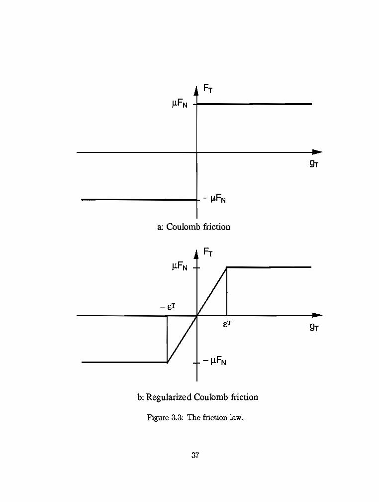
and tangential tractions are applied in opposite directions on the two surfaces in accordance with a regularized Coulomb friction law (Figure 3.3). This law, which results from modifying Coulomb's law, satisfies continuity at zero slip with a linear part over the range -ei' < 9T < cT. The variable cT is a regularization parameter (see Section 5.4). Smaller values of cT require the use of smaller step-sizes and/or more iterations, but, on the other hand, imply stiffer response in the stick case and, therefore, less relative tangential motion. The law distinguishes between two cases: Case 1: Stick condition, loTI ~cT. The tangential traction in this case is:

where p, is the coefficient of friction between the two surfaces. Case 2: Slip condition, IBTI >cT. In this case:

(3.6)

(3.7)

The application of these tractions is analogous to the addition of a tangential elastic-perfectly-plastic spring at the point.

3.3 Contact Contribution to the Virtual Work

The normal and tangential tractions (UN, UT) at a point Xc contribute to the virtual work expression by the amount:

(3.8)

36

Fr

~FN ~------------------

a: Coulomb friction

Fr

-eT

b: Regularized Coulomb friction

Figure 3.3: The friction law.

37

where the subscript c stands for contact. The virtual changes 6gN and 6gT are given by:

Equation ( 3.2) :::} 6gN = -(6Xc- 6Xoos) · n

Equation ( 3.5) => 69T = -(6Xc- 6xt) · t

However, since Xc = Xc + uc, it is clear that:

where

(3.9)

(3.10)

Xc : The position vector of point Xc in the reference configuration (constant). uc : The displacement vector of point Xc·

The reference point Xt moves with the obstacle surface; therefore:

where

Uoos : The displacement vector of point Xobs·

Vobs : Vertical displacement of the obstacle.

(3.11)

In the last equation, the fact that Uobs is a prescribed function has been ob­served. The virtual changes 6gN and 6gT become:

6gN =-(Due- Dlloos) · D

6gT = -(6Uc- 6uobs) · t (3.12)

The contribution to the virtual work expression (Equation ( 3.8)) can now be written as:

(3.13)

The contribution of contact tractions over the entire surface, r c, is found by integrating the individual contributions:

(VW)c fr c d(VW)c

- f -(6uc- 6uobs) · (O'N n + O'T t) dS (3.14) ire

38

3.4 Contact Contribution to the Finite Element Equa­tions

The linearization of the finite element equations (Equations ( 2.28)) entails contributions to both the RHS (Right Hand Side= the force vector) and the LHS (Left Hand Side= the tangent stiffness matrix). Using numerical integration over the master element, Equation ( 3.14) becomes:

N

(VW)c = 2: -wtk Jk(6u~- 6uobs) · (u~ fi. + u~ t) (3.15) k=l

where

wtk : Weight associated with integration point k. Jk : Determinant of the Jacobian of the mapping from the master-element

surface to the contact surface at integration point k. N : Number of points used in surface integration.

This gives the contact contribution to the RHS of the finite element equations. For detailed expressions in a matrix form, see Appendix A.

On the other hand, contribution to the LHS results from the direc­tional derivative of the virtual work term (Equation ( 3.15)):

N

D(VW)cfiU = 2: -wtk(6u~-6uobs)· [tiJk(u~ fi. + u~t) + Jk(fiu~ fi. + fiu~ t)] k=l

{3.16) where

(3.17)

and

fiqT = p.E~tf (fi9N9T 9Nfi9T)

= _,..E~tl (gTfi. + 9Nt) · (tiu~- fiuobs) , for I9TI :5 cT {3.18)

fiuT = J.LkN sign(9T) figN

= -J.L kN sign(9T) fi. · (fiu~ - fiuobs) , for I9TI > cT (3.19)

39

The Jacobian J and its increment tl.J along element-sides 1 and 3 (TJ = con­stant) are given by:

(3.20)

and along sides 2 and 4 (e =constant) by:

[ 2 2] 1

8x 8y 2 1 8x 8 8y 8

J = (-) + (-) ::::? tl.J = - [--(tl.x) + --(tl.y)l 8TJ 8TJ J 8TJ 8TJ 8TJ 8TJ (3.21)

where (x, y) are the coordinates of point Xc and are given by (see Equation ( 2.22)):

(3.22)

Substituting these expressions back into Equation ( 3.16) produces the contact contributions to the tangent stiffness matrix. The contact contri­bution yields nonsymmetric stiffness matrices. The matrix expressions for the individual cases are given in Appendix A.

3.5 Practical Considerations

The state of a point on the contact surface can be any of the follow­ing three states: free, stick and slip. The particular state is determined by the normal and tangential gaps at that point (gN,9T). However, to aid the con­vergence of the numerical method, some restrictions are applied to the contact condition of a point regardless of the values of 9N and 9T· Since the slip con­dition does not produce any (tangent) stiffness contribution, it is occasionally helpful to enforce a stick condition on the point. A point is held in place when an abrupt change in its contact condition is noted, as in the following cases:

• Change from free to slip.

• Change from slip to the right to slip to the left.

40

• At the first iteration in a step.

After convergence in a step, the contact condition of each (integration) point is checked. If a slip condition is detected (IBTI > c-T), the reference point XT is updated. It is translated along the obstacle surface towards xc so that IBTI =c-T.

For better representation of the contact, a trapezoidal rather than a Gaussian ru1e is used to integrate the contact equations. Different integration ru1es can be specified for different element sides along the contact surface, depending on the length of the side.

41

Chapter 4

EXAMPLES AND APPLICATIONS

4.1 Introduction

The higher-order element described in Chapter 2, along with the frictional-contact algorithm of Chapter 3, were implemented in a computer code named 'TEXPVER.' The code has been used to analyze both theoretical examples and practical applications, specifically, bridge bearing pads.

In Section 4.2, the performance of the higher-order element along with some observations about the required orders of pressure interpolation and integration rules are investigated qualitatively. It is to be emphasized that, by no means is it concluded that the proposed element is either better or worse than existing alternatives. However, the results obtained using the element in practical applications are very sound. The hierarchic shape functions combined with the nonconforming pressure modes performed satisfactorily in nonlinear rubber-elasticity problems.

Next, actual cases of bridge bearing pads are analyzed in an attempt to study the factors which affect their behavior under limiting design loads. The overall response of the pad is discussed with emphasis on its shear and compressive stiffnesses. In addition, the internal stress and strain fields are computed and contoured. Their ultimate values are found and compared. The steel laminates are observed for possible yielding.

4.2 Performance of the Higher-Order Element

The ability of the higher-order element to capture the large deforma­tions, typical of rubber, is tested in this section. Comparisons with the familiar nine-node quadratic element are shown. In addition, some examples concern­ing the appropriate choices of the order of pressure interpolation and the rule

42

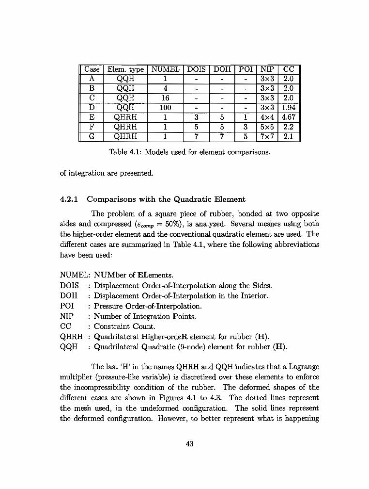
Case Elem. type NUMEL DOIS cc A QQH 2.0 B QQH 2.0 c QQH 2.0 D QQH 1.94 E QHRH 3 4.67 F QHRH 5 5x5 2.2

QHRH 7 7x7 2.1

Table 4.1: Models used for element comparisons.

of integration are presented.

4.2.1 Comparisons with the Quadratic Element

The problem of a square piece of rubber, bonded at two opposite sides and compressed {ccornp = 50%), is analyzed. Several meshes using both the higher-order element and the conventional quadratic element are used. The different cases are summarized in Table 4.1, where the following abbreviations have been used:

NUMEL: NUMber of ELements. DOIS : Displacement Order-of-Interpolation along the Sides. DOll : Displacement Order-of-Interpolation in the Interior. POI : Pressure Order-of-Interpolation. NIP : Number of Integration Points. CC : Constraint Count. QHRH : Quadrilateral Higher-ordeR element for rubber {H). QQH : Quadrilateral Quadratic {9-node) element for rubber {H).

The last 'H' in the names QHRH and QQH indicates that a Lagrange multiplier {pressure-like variable) is discretized over these elements to enforce the incompressibility condition of the rubber. The deformed shapes of the different cases are shown in Figures 4.1 to 4.3. The dotted lines represent the mesh used, in the undeformed configuration. The solid lines represent the deformed configuration. However, to better represent what is happening

43

internally, each element has been divided graphically into a specified number of quadrilaterals, originally equal squares. These quadrilaterals have been drawn over the deformed mesh.

It is clear from the deformed shapes that a single 9-node element (Case A) is not capable of representing the expected deformed shape. Case D resulted in the best deformed shape; the corner elements, however, did not behave well beyond a strain of ccomp = 30%.

Cases E, F and G use one element of the higher-order type. The displacement and pressure orders-of-interpolation as well as the integration rules are enriched from Case E to Case F to Case G. In Case E, the order of interpolation (cubic) is only one degree higher than the order in the quadratic element of Case A. It is obvious that the solution has improved considerably. In fact, it is reasonably concluded that the solution keeps improving in Cases F and G. An indication supporting this belief is that the incompressibility condition (which is translated graphically as equal areas for the quadrilaterals in the deformed configuration) is better enforced in elements with higher orders.

The other example used is a fiat piece of rubber which is glued at its top and bottom, compressed and sheared. Figure 4.4 shows the solution obtained using 20 quadratic 9-node elements. Figure 4.4 also shows the solu­tion obtained using a single higher-order element with the following properties: DOIS = 5, DOli = 7, POI = 4 and NIP = 7x7. It is evident that the two solutions are quite similar.

In conclusion, the higher-order element appears capable, with fewer number of elements than conventional elements, of modeling the nonlinear be­havior of rubber. It is relevant to add that the element has passed the constant­strain patch test.

4.2.2 Order of Pressure Interpolation

Two examples are used to study the required order of pressure inter­polation. A square piece of rubber, bonded at two opposite sides, compressed in the first example and compressed and sheared in the second, is analyzed. Three finite element models with one element each are used (see Table 4.2). While the displacement order-of-interpolation is kept constant in the three elements,

44

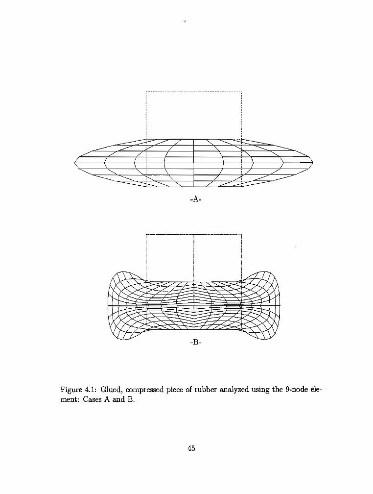
,--------·-·----------------------·-----i

-A-

' ' ' : ' ' ' i ' ' ' :

r·--·----·-·- ,----·-------~

I I ! l ! l : : :

-B-

Figure 4.1: Glued, compressed piece of rubber analyzed using the 9-node ele­ment: Cases A and B.

45

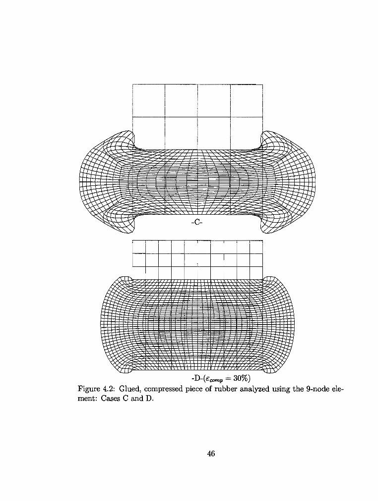
-D-(scomp = 30%) Figure 4.2: Glued, compressed piece of rubber analyzed using the 9-node ele­ment: Cases C and D.

46

~--~~-~~-----------------~-........... --------------------~

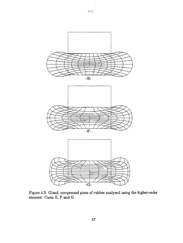
! i i ! ! i : i ! !

-E-

Figure 4.3: Glued, compressed piece of rubber analyzed using the higher-order element: Cases E, F and G.

47

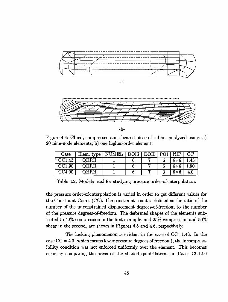
-a-

-b-

Figure 4.4: Glued, compressed and sheared piece of rubber analyzed using: a) 20 nine-node elements; b) one higher-order element.

NUMEL DOIS DOli POI NIP 1 6 7 6 6x6 1 6 7 5 6x6 1 6 7 3 6x6

Table 4.2: Models used for studying pressure order-of-interpolation.

the pressure order-of-interpolation is varied in order to get different values for the Constraint Count ( CC). The constraint count is defined as the ratio of the number of the unconstrained displacement degrees-of-freedom to the number of the pressure degrees-of-freedom. The deformed shapes of the elements sub­jected to 40% compression in the first example, and 25% compression and 50% shear in the second, are shown in Figures 4.5 and 4.6, respectively.

The locking phenomenon is evident in the case of CC=1.43. In the case CC = 4.0 (which means fewer pressure degrees of freedom), the incompress­ibility condition was not enforced uniformly over the element. This becomes clear by comparing the areas of the shaded quadrilaterals in Cases CC1.90

48

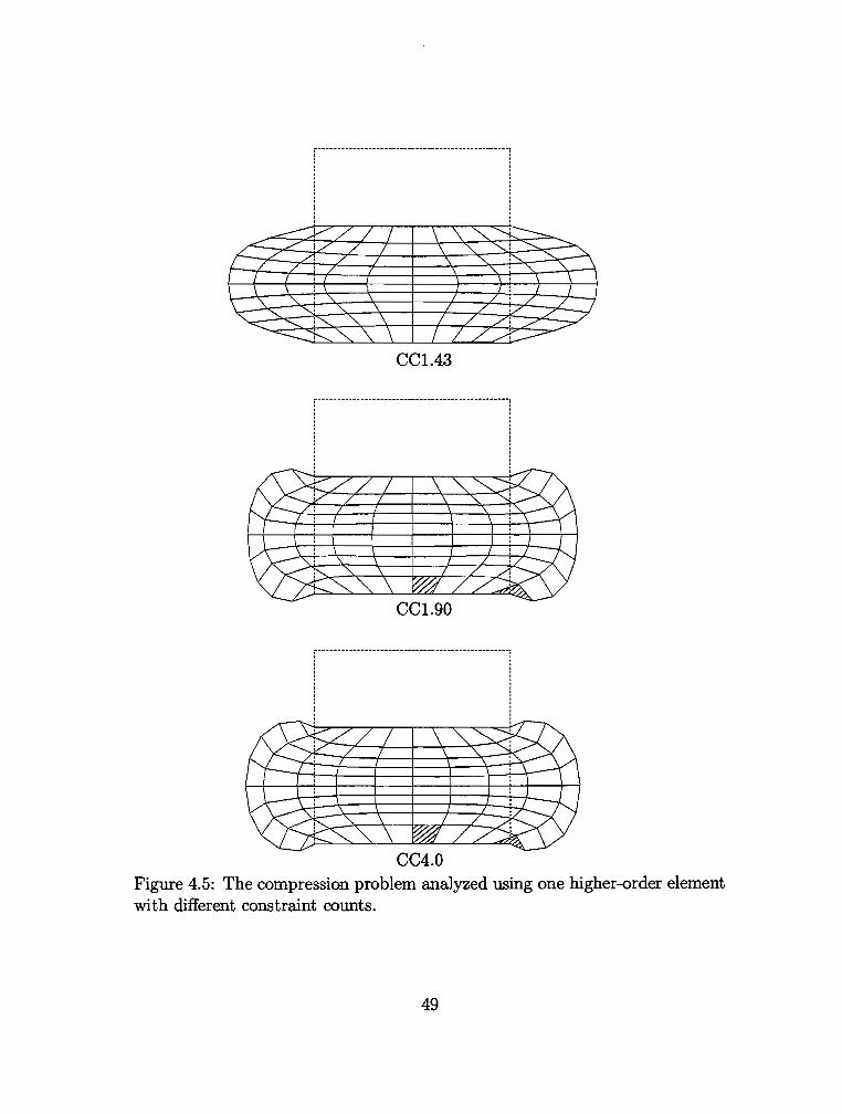
CCL43

[ ---------------------------:

i i

CCL90

_____ ...................................... ____________________________ _ ' ' ' ' ' ' ' ' ' ' ' . ' . ' ' ' . ' ' ' . ' ' ' ' ' . ' ' ' ' . ' ' ' . '

CC4.0 Figure 4.5: The compression problem analyzed using one higher-order element with different constraint counts.

49

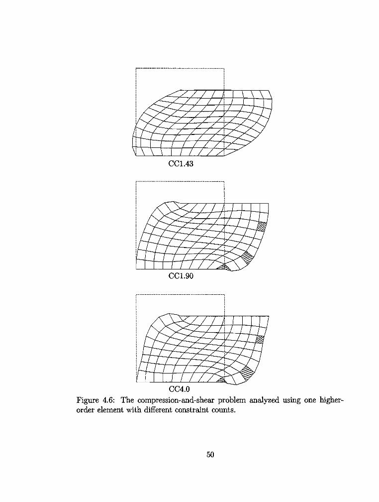
CC1.43

--------------------------------------------------· ' ' ' ' ' ' ' ' ' ' ' ' ' ' ' ' ' ' ' ' ' . ' '

'

CC1.90

----------- ---------------------------------------' ' ' ' ' ' ' ' ' ' ' . ' ' ' ' ' ' ' ' ' ' ' '

'

'

CC4.0

Figure 4.6: The compression-and-shear problem analyzed using one higher­order element with different constraint counts.

50

and CC4.00. Furthermore, the deformed shape of Case CC1.90 appears to be smoother than Case CC4.00, especially when shear is applied (Figure 4.6). The value of CC=l.9 was the closest to the optimal ratio of 2 and resulted in the best solution among the three cases (smoother and better enforcement of incompressibility).

In conclusion, Hughes' rule of thumb [36] that the pressure order-of­interpolation should be chosen so that the constraint count of the entire model comes as close as possible to 2 appears to be useful. If CC is much less than 2, the model is overconstrained, and locking becomes imminent. On the other hand, constraint counts far higher than 2 result in an underconstrained model and the incompressibility condition is underrepresented.

4.2.3 Order of Integration Rule

The problem of combined compression and shear is analyzed using one element with the following properties: DOIS 5, DOli = 7, POI= 4. The element is considered of order 5. The integration rule is a Gaussian quadrature with orders of 4x4, 5x5 and 6x6 in Cases NIP4x4, NIP5x5 and NIP6x6, respectively. The deformed shapes under 40% compression and 80% shear are shown in Figure 4. 7.

An integration rule of order less than that of the element is not enough (Case NIP4x4 converged to an absurd solution). Although Cases NIP5x5 and NIP6x6 have both converged, the deformed shape in the latter is more accurate (in Case NIP5x5, the model has flipped inside out at the lower right corner). Thus, it can be conservatively concluded that using more integration points results in better deformations, especially towards the corners.

4.3 Bridge Bearing Pads

Several cases of bridge bearing pads are analyzed. The effects of various design factors of the pad on its overall behavior as well as on stress and strain measures in both materials, rubber and steel, are discussed.

51

------------- ------------------------------------·

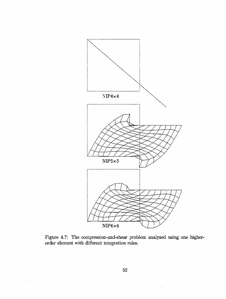
NIP4x4

'

'

'

'

[----------- -- --------------------,

~=-~~r-~------~

---------------------------------·-------------· . ' . . . . . . ' ' . ' ' ' . . . . . . . . . . . . . . ' ' . . . . . . . '

Figure 4. 7: The compression-and-shear problem analyzed using one higher­order element with different integration rules.

52

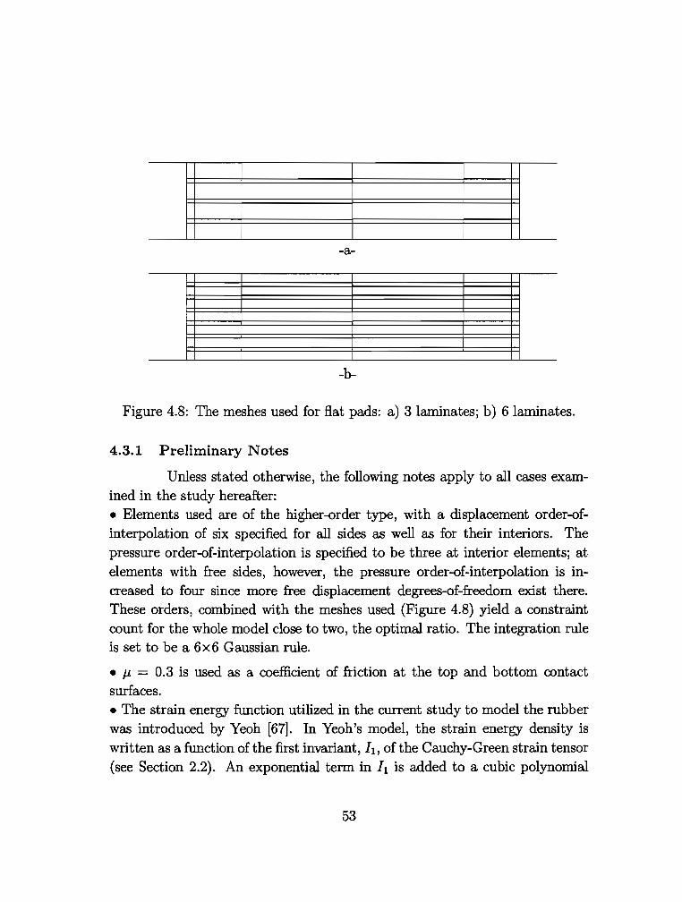
-a-

-b-

Figure 4.8: The meshes used for flat pads: a) 3 laminates; b) 6 laminates.

4.3.1 Preliminary Notes

Unless stated otherwise, the following notes apply to all cases exam­ined in the study hereafter: • Elements used are of the higher-order type, with a displacement order-of­interpolation of six specified for all sides as well as for their interiors. The pressure order-of-interpolation is specified to be three at interior elements; at elements with free sides, however, the pressure order-of-interpolation is in­creased to four since more free displacement degrees-of-freedom exist there. These orders, combined with the meshes used (Figure 4.8) yield a constraint count for the whole model close to two, the optimal ratio. The integration rule is set to be a 6x6 Gaussian rule.

• J.L = 0.3 is used as a coefficient of friction at the top and bottom contact surfaces. • The strain energy function utilized in the current study to model the rubber was introduced by Yeah [67]. In Yeah's model, the strain energy density is written as a function of the first invariant, !1, of the Cauchy-Green strain tensor (see Section 2.2). An exponential term in 11 is added to a cubic polynomial

53

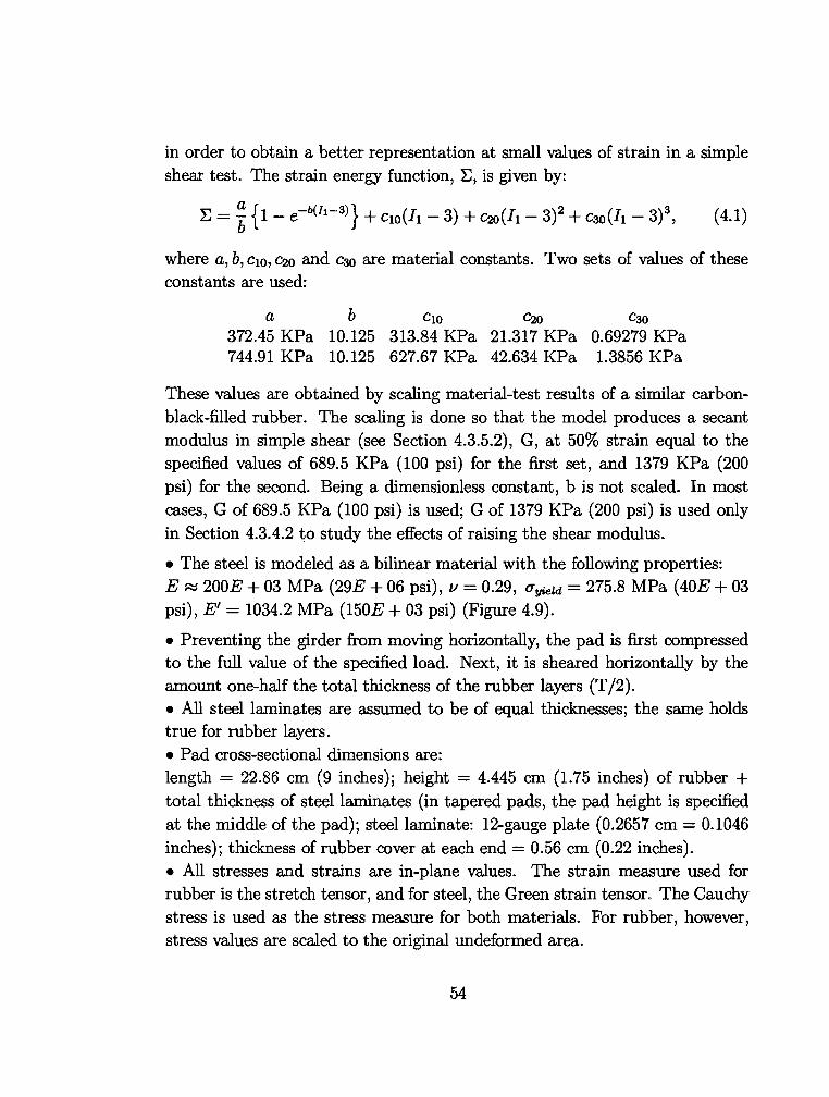
in order to obtain a better representation at small values of strain in a simple shear test. The strain energy function, E, is given by:

where a, b, cw, D.!o and C3o are material constants. Two sets of values of these constants are used:

a b cw D.!o C3o 372.45 KPa 10.125 313.84 KPa 21.317 KPa 0.69279 KPa 744.91 KPa 10.125 627.67 KPa 42.634 KPa 1.3856 KPa

These values are obtained by scaling material-test results of a similar carbon­black-filled rubber. The scaling is done so that the model produces a secant modulus in simple shear (see Section 4.3.5.2), G, at 50% strain equal to the specified values of 689.5 KPa (100 psi) for the first set, and 1379 KPa (200 psi) for the second. Being a dimensionless constant, b is not scaled. In most cases, G of 689.5 KPa (100 psi) is used; G of 1379 KPa (200 psi) is used only in Section 4.3.4.2 to study the effects of raising the shear modulus.

• The steel is modeled as a bilinear material with the following properties: E ~ 200E + 03 MPa (29E + 06 psi), v = 0.29, l1yield = 275.8 MPa (40E + 03 psi), E' = 1034.2 MPa (150E + 03 psi) (Figure 4.9).

• Preventing the girder from moving horizontally, the pad is first compressed to the full value of the specified load. Next, it is sheared horizontally by the amount one-half the total thickness of the rubber layers (T /2). • All steel laminates are assumed to be of equal thicknesses; the same holds true for rubber layers. • Pad cross-sectional dimensions are: length = 22.86 em (9 inches); height = 4.445 em (1.75 inches) of rubber + total thickness of steel laminates (in tapered pads, the pad height is specified at the middle of the pad); steel laminate: 12-gauge plate (0.2657 em= 0.1046 inches); thickness of rubber cover at each end= 0.56 em (0.22 inches). • All stresses and strains are in-plane values. The strain measure used for rubber is the stretch tensor, and for steel, the Green strain tensor. The Cauchy stress is used as the stress measure for both materials. For rubber, however, stress values are scaled to the original undeformed area.

54

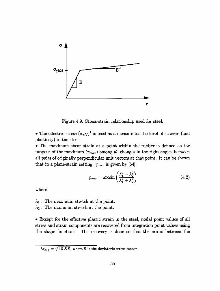
cr

O'yield E'

£

Figure 4.9: Stress-strain relationship used for steel.

• The effective stress ( u ef 1) 1 is used as a measure for the level of stresses (and plasticity) in the steel. • The maximum shear strain at a point within the rubber is defined as the tangent of the maximum (/max) among all changes in the right angles between all pairs of originally perpendicular unit vectors at that point. It can be shown that in a plane-strain setting, /m.a:r: is given by [64]:

lm.a:r: . (AI- A~) arcsm A i + A~

where

AI : The maximum stretch at the point. A2 : The minimum stretch at the point.

(4.2)

• Except for the effective plastic strain in the steel, nodal point values of all stress and strain components are recovered from integration point values using the shape functions. The recovery is done so that the errors between the

1aeff = yfl.5 S.S, where Sis the deviatoric stress tensor.

55

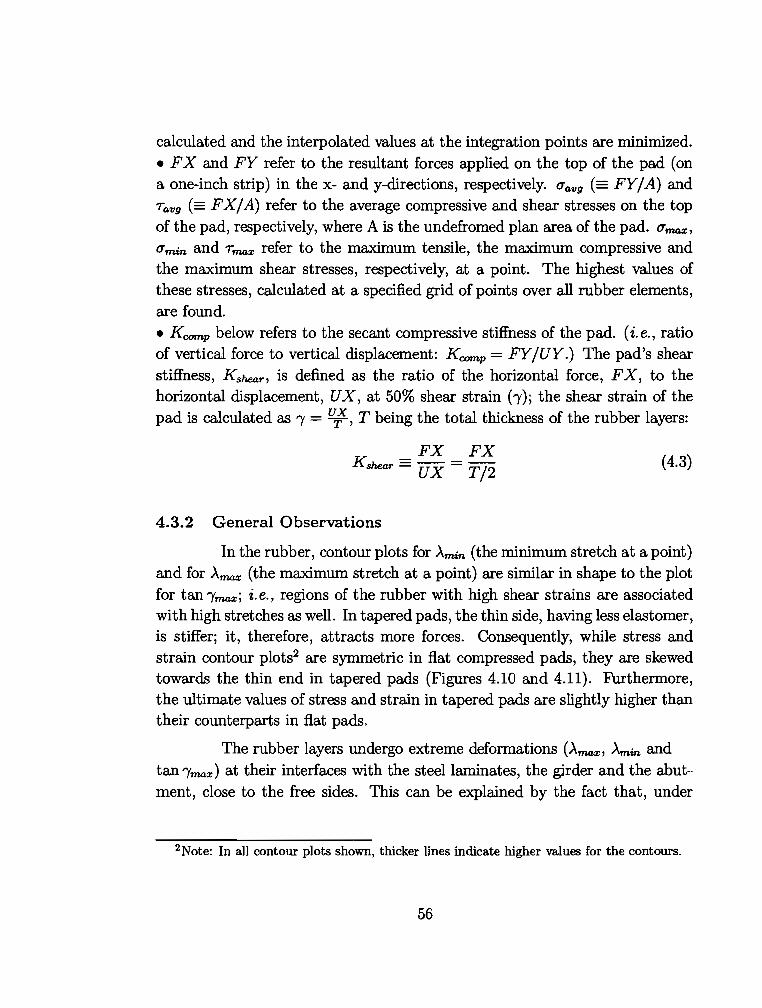
calculated and the interpolated values at the integration points are minimized. • F X and FY refer to the resultant forces applied on the top of the pad (on a one-inch strip) in the x- andy-directions, respectively. l1avg FY/A) and Tavg (= FX/A) refer to the average compressive and shear stresses on the top of the pad, respectively, where A is the undefromed plan area of the pad. l1~, l1min and r~ refer to the maximum tensile, the maximum compressive and the maximum shear stresses, respectively, at a point. The highest values of these stresses, calculated at a specified grid of points over all rubber elements, are found. • Kcmnp below refers to the secant compressive stiffness of the pad. (i.e., ratio of vertical force to vertical displacement: Kcmnp FY /UY.) The pad's shear stiffness, Kshear, is defined as the ratio of the horizontal force, F X, to the horizontal displacement, U X, at 50% shear strain ( r); the shear strain of the pad is calculated as r = u;, T being the total thickness of the rubber layers:

FX FX Kshear = UX T/2 (4.3)

4.3.2 General Observations

In the rubber, contour plots for Amm (the minimum stretch at a point) and for A~ (the maximum stretch at a point) are similar in shape to the plot for tan !max; i.e., regions of the rubber with high shear strains are associated with high stretches as well. In tapered pads, the thin side, having less elastomer, is stiffer; it, therefore, attracts more forces. Consequently, while stress and strain contour plots2 are symmetric in flat compressed pads, they are skewed towards the thin end in tapered pads (Figures 4.10 and 4.11). FUrthermore, the ultimate values of stress and strain in tapered pads are slightly higher than their counterparts in flat pads.

The rubber layers undergo extreme deformations (A~, Amm and tan !max) at their interfaces with the steel laminates, the girder and the abut­ment, close to the free sides. This can be explained by the fact that, under

2Note: In all contour plots shown, thicker lines indicate higher values for the contours.

56

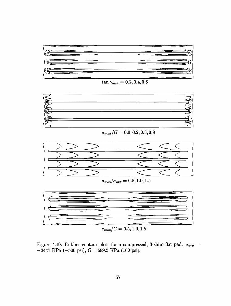
. ~ I{

i". J,

tan l'f'fUJ/X = 0.2, 0.4, 0.6

l~ ~ !b ~.

'~ 4 :~ 2

Umarr)G 0.0, 0.2, 0.5, 0.8

Umin/Uavg = 0.5, 1.0, 1.5

Figure 4.10: Rubber contour plots for a compressed, 3-shim fiat pad. Uavg = -3447 KPa ( -500 psi), G = 689.5 KPa (100 psi).

57

\ ~

~~

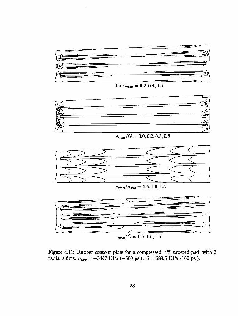
r£-

~-

1 tan ffll.a!'£ = 0.2, 0.4, 0.6

~ ~-~~ 'Lp"

= I~ ~:1 i~ ~

Umo;x/G = 0.0, 0.2, 0.5, 0.8

(

I

Figure 4.11: Rubber contour plots for a compressed, 4% tapered pad, with 3

radial shims. Uavg = -3447 KPa ( -500 psi), G = 689.5 KPa (100 psi).

58

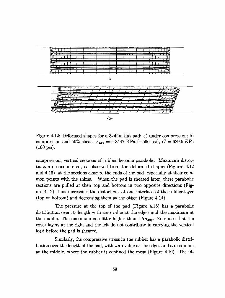
-a-

-b-

Figure 4.12: Deformed shapes for a 3-shim flat pad: a) rmder compression; b) compression and 50% shear. O'avg = -3447 KPa (-500 psi), G = 689.5 KPa (100 psi).

compression, vertical sections of rubber become parabolic. Maximum distor­tions are encountered, as observed from the deformed shapes (Figures 4.12 and 4.13), at the sections close to the ends of the pad, especially at their com­mon points with the shims. When the pad is sheared later, these parabolic sections are pulled at their top and bottom in two opposite directions (Fig­ure 4.12), thus increasing the distortions at one interface of the rubber-layer (top or bottom) and decreasing them at the other (Figure 4.14).

The pressure at the top of the pad (Figure 4.15) has a parabolic distribution over its length with zero value at the edges and the maximum at the middle. The maximum is a little higher than 1.5uavg· Note also that the cover layers at the right and the left do not contribute in carrying the vertical load before the pad is sheared.

Similarly, the compressive stress in the rubber has a parabolic distri­bution over the length of the pad, with zero value at the edges and a maximum at the middle, where the rubber is confined the most (Figure 4.10). The ul-

59

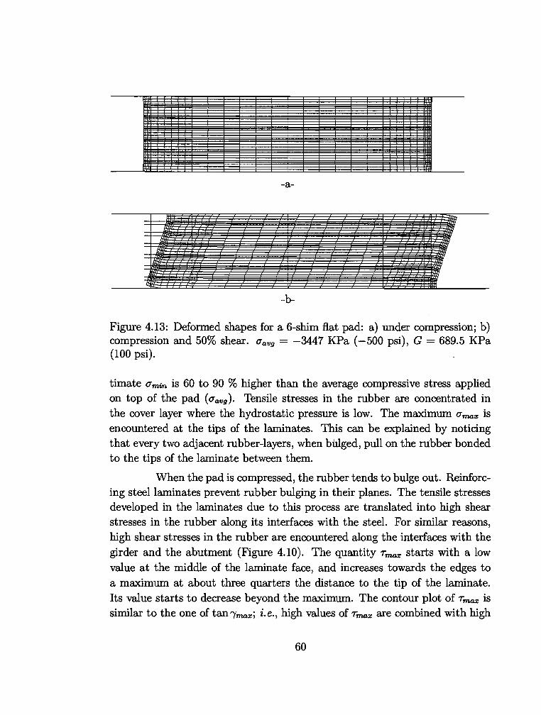
-a-

-b-

Figure 4.13: Deformed shapes for a 6-shim flat pad: a) under compression; b) compression and 50% shear. Uavg = -3447 KPa ( -500 psi), G = 689.5 KPa (100 psi).

timate u min is 60 to 90 % higher than the average compressive stress applied on top of the pad (uav9 ). Tensile stresses in the rubber are concentrated in the cover layer where the hydrostatic pressure is low. The maximum Umax is encountered at the tips of the laminates. This can be explained by noticing that every two adjacent rubber-layers, when bUlged, pull on the rubber bonded to the tips of the laminate between them.

When the pad is compressed, the rubber tends to bulge out. Reinforc­ing steel laminates prevent rubber bulging in their planes. The tensile stresses developed in the laminates due to this process are translated into high shear stresses in the rubber along its interfaces with the steel. For similar reasons, high shear stresses in the rubber are encountered along the interfaces with the girder and the abutment (Figure 4.10). The quantity 7max starts with a low value at the middle of the laminate face, and increases towards the edges to a maximum at about three quarters the distance to the tip of the laminate. Its value starts to decrease beyond the maximum. The contour plot of 7max is similar to the one of tan /maxi i.e., high values of 7max are combined with high

60

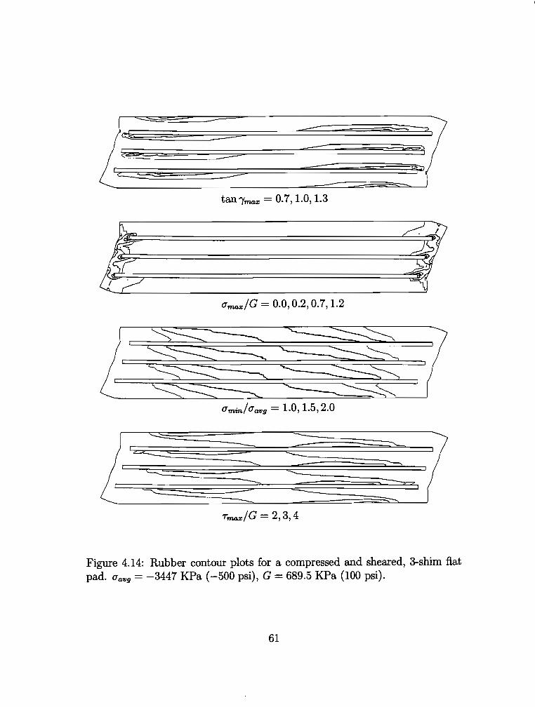
tanrmax = 0.7, 1.0, 1.3

O'max/G 0.0, 0.2, 0.7, 1.2

O'mm/O'a:vg = 1.0, 1.5, 2.0

Tmax/G = 2, 3, 4

Figure 4.14: Rubber contour plots for a compressed and sheared, 3-shim flat pad. O'avg = -3447 KPa ( -500 psi), G = 689.5 KPa (100 psi).

61

-

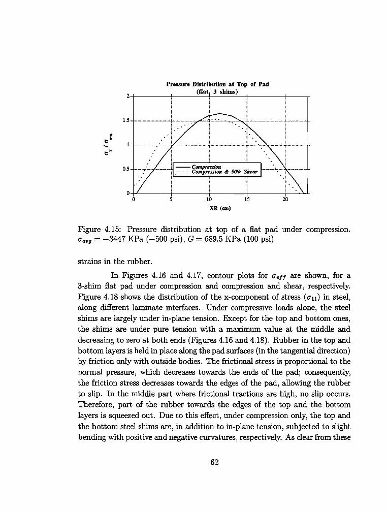
Pressure Distribution at Top of Pad (flat 3 shims)

2+-------~-------+----~~--------~---r

1.s ·······-···················r·············;··"· ~ - G . :

. l

OS .' 1 --Compression · ........ , ...... ···········: - - - - - Compression & SO% Shear ···········;····: ··········•···

. 1,, . '!-. ~ .

0~------~-------+------~--------~~~ 0 s 10 15 20

XR (CIIl)

Figure 4.15: Pressure distribution at top of a flat pad under compression. Uavg = -3447 KPa ( -500 psi), G = 689.5 KPa (100 psi).

strains in the rubber.

In Figures 4.16 and 4.17, contour plots for Ueff are shown, for a 3-shim flat pad under compression and compression and shear, respectively. Figure 4.18 shows the distribution of the x-component of stress (u11) in steel, along different laminate interfaces. Under compressive loads alone, the steel shims are largely under in-plane tension. Except for the top and bottom ones, the shims are under pure tension with a maximum value at the middle and decreasing to zero at both ends (Figures 4.16 and 4.18). Rubber in the top and bottom layers is held in place along the pad surfaces (in the tangential direction) by friction only with outside bodies. The frictional stress is proportional to the normal pressure, which decreases towards the ends of the pad; consequently, the friction stress decreases towards the edges of the pad, allowing the rubber to slip. In the middle part where frictional tractions are high, no slip occurs. Therefore, part of the rubber towards the edges of the top and the bottom layers is squeezed out. Due to this effect, under compression only, the top and the bottom steel shims are, in addition to in-plane tension, subjected to slight bending with positive and negative curvatures, respectively. As clear from these

62

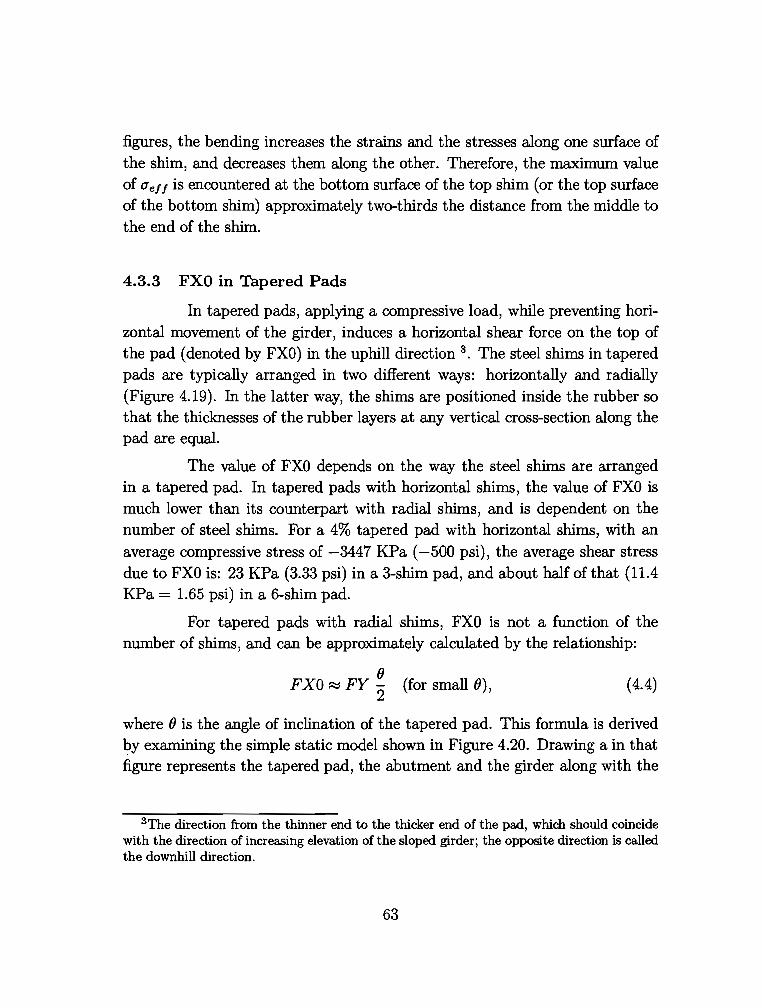
figures, the bending increases the strains and the stresses along one surface of the shim, and decreases them along the other. Therefore, the maximum value of a ef 1 is encountered at the bottom surface of the top shim (or the top surface of the bottom shim) approximately two-thirds the distance from the middle to the end of the shim.

4.3.3 FXO in Tapered Pads

In tapered pads, applying a compressive load, while preventing hori­zontal movement of the girder, induces a horizontal shear force on the top of the pad (denoted by FXO) in the uphill direction 3. The steel shims in tapered pads are typically arranged in two different ways: horizontally and radially (Figure 4.19). In the latter way, the shims are positioned inside the rubber so that the thicknesses of the rubber layers at any vertical cross-section along the pad are equaL

The value of FXO depends on the way the steel shims are arranged in a tapered pad. In tapered pads with horizontal shims, the value of FXO is much lower than its counterpart with radial shims, and is dependent on the number of steel shims. For a 4% tapered pad with horizontal shims, with an average compressive stress of -3447 KPa ( -500 psi), the average shear stress due to FXO is: 23 KPa (3.33 psi) in a 3-shim pad, and about half of that (11.4 KPa = 1.65 psi) in a 6-shim pad.

For tapered pads with radial shims, FXO is not a function of the number of shims, and can be approximately calculated by the relationship:

(} FXO ~ FY 2 (for small 0), (4.4)

where (} is the angle of inclination of the tapered pad. This formula is derived by examining the simple static model shown in Figure 4.20. Drawing a in that figure represents the tapered pad, the abutment and the girder along with the

3The direction from the thinner end to the thicker end of the pad, which should coincide with the direction of increasing elevation of the sloped girder; the opposite direction is called the downhill direction.

63

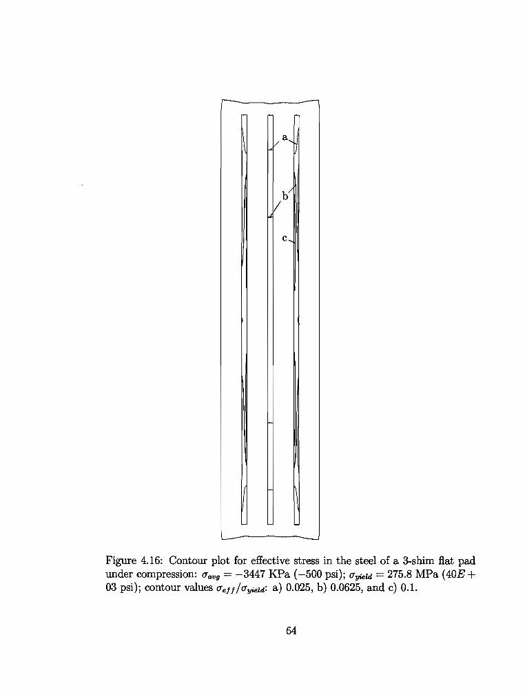
a

b

c

Figure 4.16: Contour plot for effective stress in the steel of a 3-shim flat pad under compression: qavg = -3447 KPa (-500 psi); qyield = 275.8 MPa (40E+ 03 psi); contour values qefffqyield: a) 0.025, b) 0.0625, and c) 0.1.

64

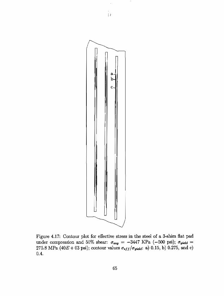
a b

c

Figure 4.17: Contour plot for effective stress in the steel of a 3-shim fiat pad under compression and 50% shear: Ua:vg = -3447 KPa ( -500 psi}; Uyie!.d = 275.8 MPa (40E+03 psi); contour values Uett/Uyield: a) 0.15, b) 0.275, and c) 0.4.

65

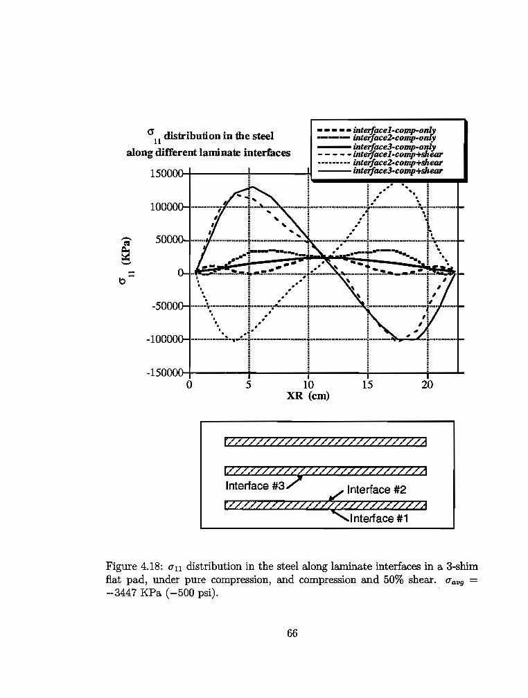
0'11

distribution in dte steel

along different laminate interfaces

• • • • • interf..acel-comp-on(y ·--- inteiface2-comp-onfy --- interf..ace3-comp-only - - - -- inteif_acel-comp+sheor

-~ ---0

•••• ••• ·- inteiface2-comp+sheor

15~~r-------------r-------------~:::::~~:;~ac;e~~;c~o;mp:;+sh.:;eor~ .. ~ : .· ·.

0 5

: .· '• § i .·· ·-. ~

··-·-~ ............................... :r--·····-···· .... -s--·-· .. . i .:! .,

! __ ....... :, .. ::~+-·-·-P"·-

10 XR (em)

......... ..-... : . : ... : ·. ........ . : .

15 20

rZZZVZZZZZ77ZZZZZVVZZ%ZZ22!

ez~WVVVZZVZA Interface #3 Interface #2

~ Figure 4.18: uu distribution in the steel along laminate interfaces in a 3-shlm fiat pad, under pure compression, and compression and 50% shear. Uavg = -3447 KPa ( -500 psi). ·

66

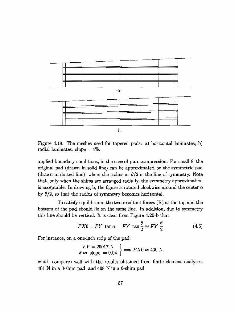
. -a-

-b-

Figure 4.19: The meshes used for tapered pads: a) horizontal laminates; b) radial laminates. slope= 4%.

applied boundary conditions, in the case of pure compression. For small(), the original pad (drawn in solid line) can be approximated by the symmetric pad (drawn in dotted line), where the radius at 8/2 is the line of symmetry. Note that, only when the shims are arranged radially, the symmetry approximation is acceptable. In drawing b, the figure is rotated clockwise around the center o by () /2, so that the radius of symmetry becomes horizontal.

To satisfy equilibrium, the two resultant forces (R) at the top and the bottom of the pad should lie on the same line. In addition, due to symmetry this line should be verticaL It is clear from Figure 4.20-b that:

() () F XO = FY tan a = FY tan- ~ FY - ( 4.5)

2 2

For instance, on a one-inch strip of the pad:

FY = 20017 N } ==> FXO ~ 400 N () ~ slope 0.04 '

which compares well with the results obtained from finite element analyses: 401 Nina 3-shim pad, and 408 Nina 6-shim pad.

67

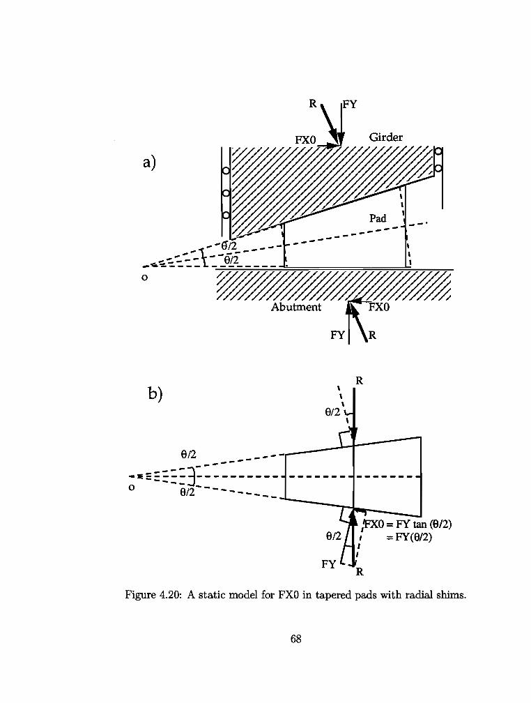
FY

a)

Abutment

b)

----------·===::3::: ______ _ .................. 0 8/2 ........ - .... - - - - - -

8/2

FY

FY

R

1'FXO = FY tan (8/2)

=FY(8/2)

R

Figure 4.20: A static model for FXO in tapered pads with radial shims.

68

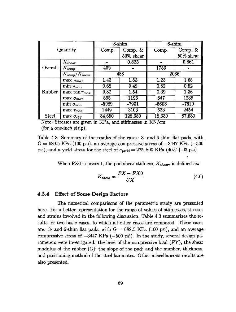
3-shim 6-shim Quantity Comp. Comp. & Comp.

50% shear Kshear - 0.823 -

Overall Kcamp 402 - I 1753

Kcamp/ Kshear 488 max Ama.x 1.43 1.83 1.23 min Amin 0.68 0.49 0.82

Rubber max tan1ma.x 0.82 1.54 0.39 max Uma.x 895 1193 647 min Umin -5989 -7901 -5603 max Tma.x 1449 3103 633

Steel max Uef! 34,650 128,380 18,330 Note: Stresses are given m KPa, and stiffnesses m KN/cm (for a one-inch strip).

Comp. & 50% shear

0.861 -

2036 1.68 0.52 1.36 II

. 1238 -7619 2454

87,630

Table 4.3: Summary of the results of the cases: 3- and 6-shim flat pads, with G = 689.5 KPa (100 psi), an average compressive stress of -3447 KPa (-500 psi), and a yield stress for the steel of Uyiezd = 275,800 KPa (40E + 03 psi).

When FXO is present, the pad shear stiffness, Kshear, is defined as:

FX-FXO ux

4.3.4 Effect of Some Design Factors

(4.6)

The numerical comparisons of the parametric study are presented here. For a better representation for the range of values of stiffnesses, stresses and strains involved in the following discussion, Table 4.3 summarizes there­sults for two basic cases, to which all other cases are compared. These cases are: 3- and 6-shim flat pads, with G = 689.5 KPa (100 psi), and an average compressive stress of -3447 KPa ( -500 psi). In the study, several design pa­rameters were investigated: the level of the compressive load (FY); the shear modulus of the rubber (G); the slope of the pad; and the number, thickness, and positioning method of the steel laminates. Other miscellaneous results are also presented.

69

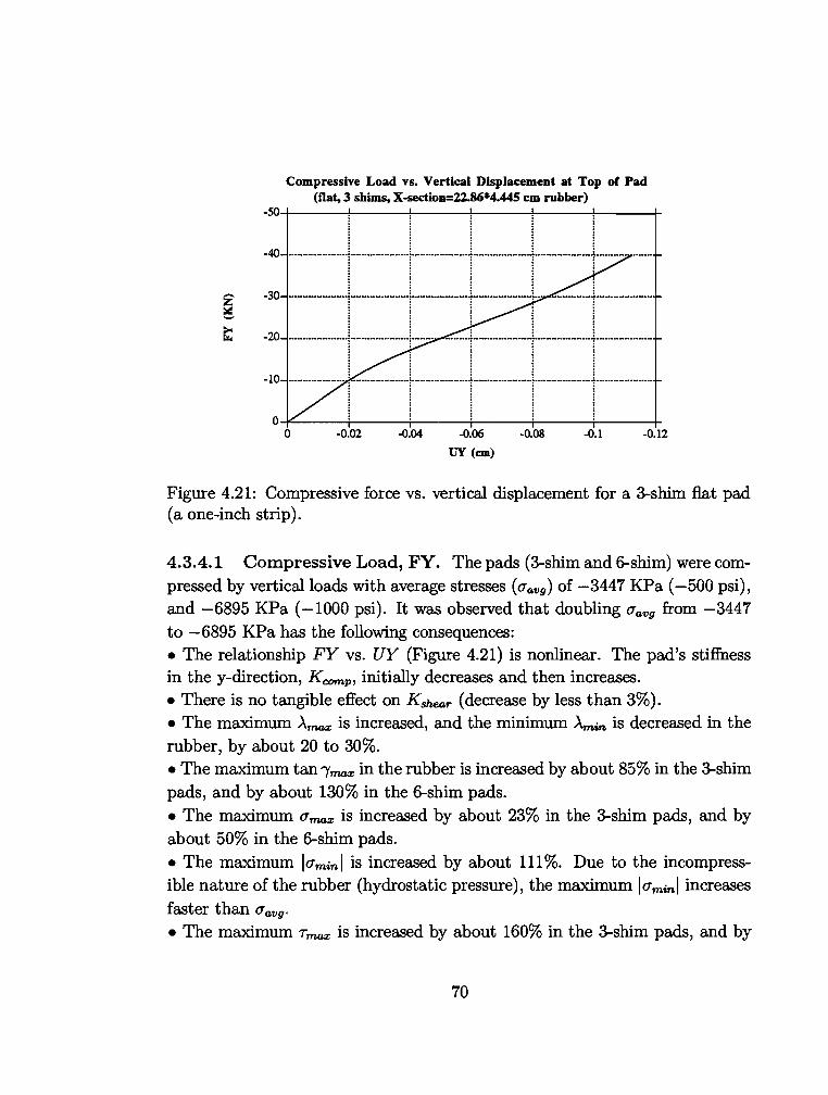
Compressive Load vs. Vertical Displacement at Top of Pad (flat, 3 shims, X-section=2l.86*4.445 em rubber)

-50+----+-----+-----+--~r---+---+

40 : : : : :

:,. =··+·: .. ~~+.:~=·· :: =~·:=t~~::~=t=~.d=

I I I I I 0~-----r---r--~---~r---r---+

0 -0.02 -0.04 -0.06

UY (em)

-0.08 -0.1 -0.12

Figure 4.21: Compressive force vs. vertical displacement for a 3-shim flat pad (a one-inch strip).

4.3.4.1 Compressive Load, FY. The pads (3-shim and 6-shim) were com­pressed by vertical loads with average stresses (o-avg) of -3447 KPa (-500 psi), and -6895 KPa ( -1000 psi). It was observed that doubling O"avg from -3447 to -6895 KPa has the following consequences: • The relationship FY vs. UY (Figure 4.21) is nonlinear. The pad's stiffness in they-direction, Kcomp, initially decreases and then increases. • There is no tangible effect on Kshear (decrease by less than 3%). • The maximum Amax is increased, and the minimum Amin is decreased in the rubber, by about 20 to 30%. • The maximum tan /max in the rubber is increased by about 85% in the 3-shim pads, and by about 130% in the 6-shim pads. • The maximum O"max is increased by about 23% in the 3-shim pads, and by about 50% in the 6-shim pads. • The maximum luminl is increased by about 111%. Due to the incompress­ible nature of the rubber (hydrostatic pressure), the maximum luminl increases faster than O"avg·

• The maximum Tmax is increased by about 160% in the 3-shim pads, and by

70

about 320% in the 6-shim pads. • The maximum O'eff is increased in the steel by about 108%.

4.3.4.2 Shear Modulus of Rubber, G. Two values for the (material) shear modulus have been used in 3-shim flat pads: 689.5 KPa (100 psi) and 1379 KPa (200 psi). Increasing G by a 100% has the following effects: • Kcomp is increased by about 150%. • Kshear is increased by about 97%. • The maximum .A'/'114X and the minimum Amin in the rubber are reduced by about 20 to 30%. • The maximum tan /rrw.z in the rubber is reduced by about 70%. • The maximum O'rrw.z is increased by about 32%. • Since the vertical load is specified, the increase in G does not have consider­able effect on the ultimate O'min (about 5% decrease). • The maximum Trrw.z is reduced by about 45%. • The maximum O'eff is reduced by about 17%.

4.3.4.3 Flat vs. Tapered Pads. Changing the slope of the top surface of the pad from 0% (flat pad) to 4% (tapered pad) leads to: • A slight decrease in Kcomp: about 5 to 10% in the 3-shim pads, and about 20% in the 6-shim pads. • A very small (less than 4%) effect on Kshear·

• An increase of less than 10% in the maximum and the minimum stretches in the rubber. • An increase in the maximum tan /rrw.z in the rubber of about 7 to 12% in the 3-shim pads, and of about 50% in the 6-shim pads. • An increase in the maximum a'/'114X in the rubber of about 7% in the 3-shim pads, and of about 20% in the 6-shim pads. • An increase of about 5 to 10% in the maximum Iammi· • An increase in the maximum Trrw.z in the rubber of about 25% in the 3-shim pads, and of about 50% in the 6-shim pads. • An increase in the maximum O'eff in the steel of about 10% in the 3-shim pads, and of about 15 to 25% in the 6-shim pads.

71

4.3.4.4 Number of Steel Laminates. Two different pads are compared: one with three 12-gauge shims, and the other with six shims of the same gauge. The total thickness of rubber is kept the same and is evenly divided between the layers. The increase in the number of laminates from three to six has the following effects: • It has a paramount effect on Kcomp (increase by about 270 to 340%). • Kshear is slightly increased (about 5%). • Extreme values of Amax and Amin in the rubber are reduced by 10 to 20%; this, in turn, implies a reduction in the maximum stresses in the rubber. • The maximum tan lm.az is reduced by 30 to 50%. • The maximum cr ma::c in the rubber is decreased by about 17 to 28%. • The maximum lcrminl in the rubber is decreased by about 6%. • The maximum Tma::c in the rubber is decreased by about 40 to 55%. • The maximum CTeff in the steel is decreased by about 45%.

4.3.4.5 Thickness of Steel Laminates. Keeping everything else the same in a 3-shim flat pad, 3 different thicknesses of the steel laminates have been tried: 10-gauge (0.3416 em), 12-gauge (0.2657 em) and 14-gauge (0.1897 em). It is concluded that, as long as the laminates are thick enough (as in the sizes chosen) to prevent yielding, changing the laminate thickness has no effect on the compressive and shear stiffnesses of the pad. Similarly, it does not have any tangible effect on the strains, CTmin or Tmax in the rubber. The only effects observed are: • Maximum tensile stresses in the rubber are concentrated in the cover layer at the tips of the laminates. By increasing the laminate thickness, CTm.az is decreased. Likewise, the maximum CTeff in the steel is obviously decreased by increasing the thickness of the shims:

t: 0.1897 .-....+

Maximumcrmax/G: 1.40 -+

MaximumCTeff/CTyield: 0.1452 -+

0.2657 -+

1.30 -+

0.1256 -+

0.3416 em 1.24

0.1122

4.3.4.6 Positioning of Steel Laminates (horizontal vs. radial) in Ta­pered Pads. As explained above, the steel laminates in tapered pads can be arranged in the cross section either radially or horizontally.

72

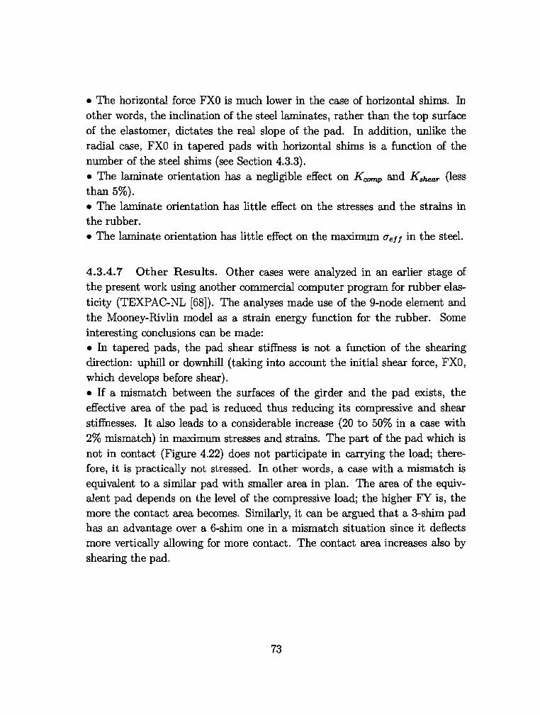
• The horizontal force FXO is much lower in the case of horizontal shims. In other words, the inclination of the steel laminates, rather than the top surface of the elastomer, dictates the real slope of the pad. In addition, unlike the radial case, FXO in tapered pads with horizontal shims is a function of the number of the steel shims (see Section 4.3.3). • The laminate orientation has a negligible effect on Kcamp and Kshear (less than 5%). • The laminate orientation has little effect on the stresses and the strains in the rubber. • The laminate orientation has little effect on the maximum u ef 1 in the steel.

4.3.4. 7 Other Results. Other cases were analyzed in an earlier stage of the present work using another commercial computer program for rubber elas· ticity {TEXPAC.NL [68]). The analyses made use of the 9-node element and the Mooney·Rivlin model as a strain energy function for the rubber. Some interesting conclusions can be made: • In tapered pads, the pad shear stiffness is not a function of the shearing direction: uphill or downhill (taking into account the initial shear force, FXO, which develops before shear). • If a mismatch between the surfaces of the girder and the pad exists, the effective area of the pad is reduced thus reducing its compressive and shear stiffnesses. It also leads to a considerable increase {20 to 50% in a case with 2% mismatch) in maximum stresses and strains. The part of the pad which is not in contact (Figure 4.22) does not participate in carrying the load; there· fore, it is practically not stressed. In other words, a case with a mismatch is equivalent to a similar pad with smaller area in plan. The area of the equiv­alent pad depends on the level of the compressive load; the higher FY is, the more the contact area becomes. Similarly, it can be argued that a 3-shim pad has an advantage over a 6·shim one in a mismatch situation since it deflects more vertically allowing for more contact. The contact area increases also by shearing the pad.

73

- -

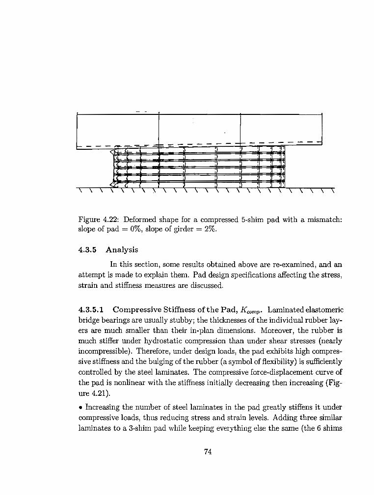
..... =--=,...::- = =-- - - ..._ --- ---- . < il-

<.; (

\ \ \ \ \ \ \ \ \ \ \ \ \ \ \ \ \ \ \ \ \ \

Figure 4.22: Deformed shape for a compressed 5-shim pad with a mismatch: slope of pad 0%, slope of girder= 2%.

4.3.5 Analysis

In this section, some results obtained above are re-examined, and an attempt is made to explain them. Pad design specifications affecting the stress, strain and stiffness measures are discussed.

4.3.5.1 Compressive Stiffness of the Pad, Kcamp· Laminated elastomeric bridge bearings are usually stubby; the thicknesses of the individual rubber lay­ers are much smaller than their in-plan dimensions. Moreover, the rubber is much stiffer under hydrostatic compression than under shear stresses (nearly incompressible). Therefore, under design loads, the pad exhibits high compres­sive stiffness and the bulging of the rubber (a symbol of flexibility) is sufficiently controlled by the steel laminates. The compressive force-displacement curve of the pad is nonlinear with the stiffness initially decreasing then increasing (Fig­ure 4.21).

• Increasing the number of steel laminates in the pad greatly stiffens it under compressive loads, thus reducing stress and strain levels. Adding three similar laminates to a 3-shim pad while keeping everything else the same (the 6 shims

74

are evenly spaced throughout the thickness of the pad), raises Kcomp by about 270 to 340%.

• The shear modulus of the Rubber, G, has a significant effect on Koomp:

G : 689.5 KPa (100 psi) --+ 1379 KPa (200 psi) ==:::;.. Kcomp increases by about 150%

• Tapered pads have slightly lower Kcomp than the flat pads:

1 0 4(]'1 { 5 to 10% decrease in 3-shim pads.

s ope : --+ IO ==> 20(]'1 d . 6- hi ads 10 ecrease m s m p .

4.3.5.2 Shear Stiffness of the Pad, Kshear· In this section, the ideal simple shear is discussed first. Then, the case of a glued pad is analyzed. Finally, the case of a real pad sheared by friction forces is presented. & shown shortly, the secant shear modulus is reduced going from the first to the second to the third case.

The ideal simple shear (Figure 4.23) is a homogeneous state of defor­mations with a deformation gradient tensor, F, given by [64]:

[ 1 1 0 l F= 0 1 0 , 0 0 1

(4.7)

where 1 =tan e = ~::.; is the shear strain. In simple shear, in addition to the shear force, a tensile force is required to maintain the thickness, T, constant throughout the deformation. Simple shear cannot be obtained exactly due to the state of the boundary conditions at the corners (Figure 4.23). In practice, however, the experiment is done on a flat piece of rubber with thickness-to­length ratio small enough to neglect the end effects.

From Equation ( 4. 7) above, the right Cauchy-Green strain tensor is obtained as:

(4.8)

Therefore, (4.9)

75

~

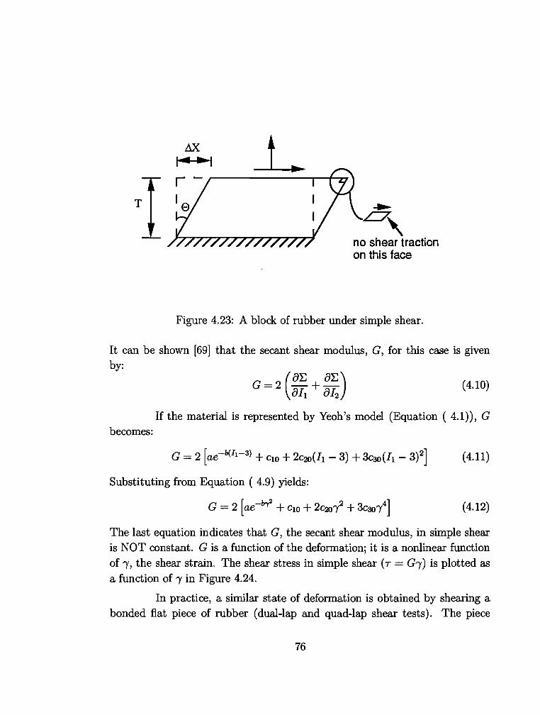
L:7' no shear traction on this face

Figure 4.23: A block of rubber under simple shear.

It can be shown [69] that the secant shear modulus, G, for this case is given by:

(4.10)

If the material is represented by Yeoh's model (Equation ( 4.1)), G becomes:

G = 2 [ae-b(h-a) + cw + 2c20(h- 3) + 3cao(Jl- 3)2] (4.11)

Substituting from Equation ( 4.9) yields:

(4.12)

The last equation indicates that G, the secant shear modulus, in simple shear is NOT constant. G is a function of the deformation; it is a nonlinear function of 1, the shear strain. The shear stress in simple shear ( T = G1) is plotted as a function of 1 in Figure 4.24.

In practice, a similar state of deformation is obtained by shearing a bonded fiat piece of rubber (dual-lap and quad-lap shear tests). The piece

76

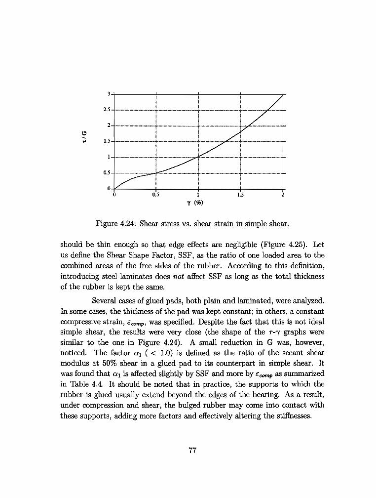
3;-------~--------~--------~-------r

2.5 ·-· t--·-j--········-t-···········-· ·······-: : :

2 ·················-·············t················--····--1--··········-·········- ~--·· ·····················-·

1.5 --·····················-+--·----··-·········-·-···1···-···-·-··-· ········f···········-·--·-······ : : :

~ I i

.~ ==r:=-=:::.r===F~=::= 0~------~--------~--------~-------+

0 0.5 1 1.5 2

r (%)

Figure 4.24: Shear stress vs. shear strain in simple shear.

should be thin enough so that edge effects are negligible {Figure 4.25). Let us define the Shear Shape Factor, SSF, as the ratio of one loaded area to the combined areas of the free sides of the rubber. According to this definition, introducing steel laminates does not affect SSF as long as the total thickness of the rubber is kept the same.

Several cases of glued pads, both plain and laminated, were analyzed. In some cases, the thickness of the pad was kept constant; in others, a constant compressive strain, C:comv, was specified. Despite the fact that this is not ideal simple shear, the results were very close (the shape of the r-r graphs were similar to the one in Figure 4.24). A small reduction in G was, however, noticed. The factor a 1 ( < 1.0) is defined as the ratio of the secant shear modulus at 50% shear in a glued pad to its counterpart in simple shear. It was found that a 1 is affected slightly by SSF and more by C:comp as summarized in Table 4.4. It should be noted that in practice, the supports to which the rubber is glued usually extend beyond the edges of the bearing. As a result, under compression and shear, the bulged rubber may come into contact with these supports, adding more factors and effectively altering the stiffnesses.

77

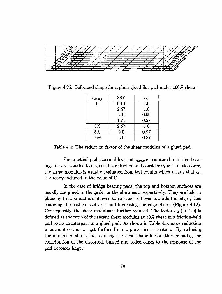
Figure 4.25: Deformed shape for a plain glued flat pad under 100% shear.

€camp SSF Ql

0 5.14 1.0 2.57 1.0 2.0 0.99 1.71 0.98

3% 2.57 1.0 5% 2.0 0.97 10% 2.0 0.87

Table 4.4: The reduction factor of the shear modulus of a glued pad.

For practical pad sizes and levels of ecornp encountered in bridge bear­ings, it is reasonable to neglect this reduction and consider a 1 ~ 1.0. Moreover, the shear modulus is usually evaluated from test results which means that a1

is already included in the value of G.

In the case of bridge bearing pads, the top and bottom surfaces are usually not glued to the girder or the abutment, respectively. They are held in place by friction and are allowed to slip and roll-over towards the edges, thus changing the real contact area and increasing the edge effects (Figure 4.12). Consequently, the shear modulus is further reduced. The factor a 2 ( < 1.0) is defined as the ratio of the secant shear modulus at 50% shear in a friction-held pad to its counterpart in a glued pad. As shown in Table 4.5, more reduction is encountered as we get further from a pure shear situation. By reducing the number of shims and reducing the shear shape factor (thicker pads), the contribution of the distorted, bulged and rolled edges to the response of the pad becomes larger.

78

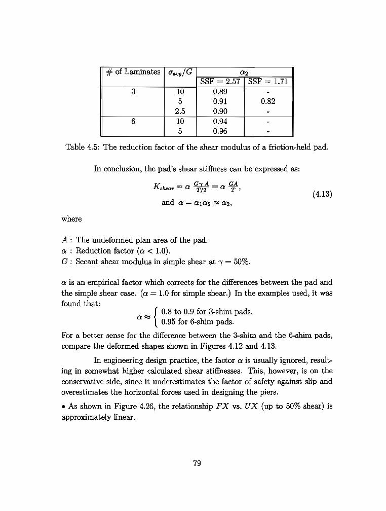
# of Laminates C!avg/G a2 SSF = 2.57 SSF 1.71

3 10 0.89 -5 0.91 0.82

2.5 0.90 -6 10 0.94 -

5 0.96 -Table 4.5: The reduction factor of the shear modulus of a friction-held pad.

In conclusion, the pad's shear stiffness can be expressed as:

K _ G1A _ GA shear - a T/2 - a T'

and a= a1a2 ~ a2,

where

A : The undeformed plan area of the pad. a : Reduction factor (a< 1.0). G : Secant shear modulus in simple shear at 1 = 50%.

(4.13)

a is an empirical factor which corrects for the differences between the pad and the simple shear case. (a= 1.0 for simple shear.) In the examples used, it was found that:

{ 0.8 to 0.9 for 3-shim pads.

a~ 0.95 for 6-shim pads.

For a better sense for the difference between the 3-shim and the 6-shim pads, compare the deformed shapes shown in Figures 4.12 and 4.13.

In engineering design practice, the factor a is usually ignored, result­ing in somewhat higher calculated shear stiffnesses. This, however, is on the conservative side, since it underestimates the factor of safety against slip and overestimates the horizontal forces used in designing the piers.

• As shown in Figure 4.26, the relationship FX vs. UX (up to 50% shear) is approximately linear.

79

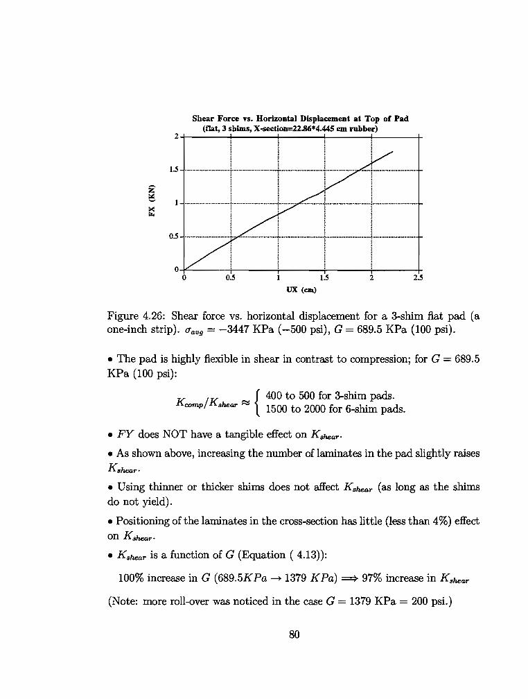
Shear Force vs. Horizontal Displacement at Top of Pad (flat. 3 shims, X-seetion=22.86*4.445 em rubber)

2+-----~~----~------4-----~-------+

!

1.5 ·························t-·····················t .... --.. - ....... +················ ·····!························· ~ i ~ ~

I ......................... 1 ....................... .1 ... ___ _ ______ : ....................... ..1 .......... -····-·· ..

I i ! ! 0.5 ·········------------- ········-··-······--···----·-->···············--····•····--···--··-··-: : :

I I I i ~ ~

0~----~r------+------+-----~-------+ 0 0.5 1.5 2 2.5

UX (em)

Figure 4.26: Shear force vs. horizontal displacement for a 3-shim flat pad (a one-inch strip). qa:vg = -3447 KPa ( -500 psi), G = 689.5 KPa (100 psi).

• The pad is highly flexible in shear in contrast to compression; for G = 689.5 KPa (100 psi):

{ 400 to 500 for 3-shim pads.

Kcomp/ Kshear ~ 1500 to 2000 for 6-shim pads.

• FY does NOT have a tangible effect on Ks~~ear-

• As shown above, increasing the number of laminates in the pad slightly raises

Kshear•

• Using thinner or thicker shims does not affect Kshear (as long as the shims do not yield).

• Positioning of the laminates in the cross-section has little (less than 4%) effect on Ks~~ear-

• Kshear is a function of G (Equation ( 4.13)):

100% increase in G (689.5KPa--+ 1379 KPa) ==} 97% increase in Kshear

(Note: more roll-over was noticed in the case G = 1379 KPa 200 psi.)

80

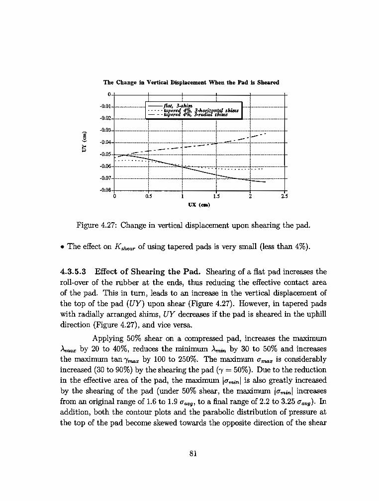
The Change in Vertical Displa<:emeot When the Pad is Sheared

0+-------~-----+------~------~-----+

-0.01 ··-···········--·· --flat, 3-shim ... .l .. ·-···················· • · · - · tapered 4'§!, 3-horiZPntaJ shims i - - -tapered 4%; 3-radwl shims :

-0.02 ----·----- l : : ···t···············-···· -0.03 ....................... .l . .__ ................ ._l ______________ J __________________ l_ _______________ _

~04 -~-:-1:-===i==··~==-f--~:c:::t:~---0.05 ········-·•············-········--.-..----·········!················--·-.-..---·····-··············· -0.06 : .. :.: .. : .. :.: .. :.: . .:..:.( .. :.: .. :.... _____ . ~ '·'·----.··:-:··:··j·:··:·:··;·:··:··:·:··:·J:-·:-:-::················ -0.07 ......................... .l. ....................... .l ......................... ~·-·········· .... 1. ....................... .

~ ~ ~ -0.08+-------i-------+-------+-------+-------+ 0 0.5 1.5 2 2.5

UX (em)

Figure 4.27: Change in vertical clisplacement upon shearing the pad.

• The effect on Kshear of using tapered pads is very small (less than 4%).

4.3.5.3 Effect of Shearing the Pad. Shearing of a flat pad increases the roll-over of the rubber at the ends, thus reducing the effective contact area of the pad. This in turn, leads to an increase in the vertical clisplacement of the top of the pad (UY) upon shear (Figure 4.27). However, in tapered pads with raclially arranged shims, UY decreases if the pad is sheared in the uphill direction (Figure 4.27), and vice versa.

Applying 50% shear on a compressed pad, increases the maximum Ama.x by 20 to 40%, reduces the minimum Amin by 30 to 50% and increases the maximum tan "fmo.x by 100 to 250%. The maximum Umax is considerably increased (30 to 90%) by the shearing the pad ('y 50%). Due to the reduction in the effective area of the pad, the maximum luminl is also greatly increased by the shearing of the pad (under 50% shear, the maximum luminl increases from an original range of 1.6 to 1.9 Ua119 , to a final range of 2.2 to 3.25 Ua119 ). In adclition, both the contour plots and the parabolic clistribution of pressure at the top of the pad become skewed towards the opposite clirection of the shear

81

(Figure 4.15).

Furthermore, as explained earlier, when the parabolic cross-sections of the right half of a rubber layer are sheared to the right, the strains decrease at their top and increase at their bottom. This, leads to the release of high shear stresses at the top interfaces and to their increase at the bottom interfaces. The opposite happens at the left half of the pad. Maximum Tmax is increased by about 100 to 200% or even more upon the application of a 50% shear strain.

When the pad is sheared, all shims are bent. Since the shims are rel­atively thin, bending will have high impact on the stresses and strains in them (Figures 4.16, 4.17, and 4.18). By applying 50% shear after compression, the maximum Ueff increases in the following manner: In 3-shim pads, it increases from an original range of 0.13 to 0.26 u!field to a final range of 0.47 to 0. 75 u!fieldi

in 6-shim pads, it increases from an original range of 0.07 to 0.14 Uyield to a final range of 0.32 to 0.46 uyield.

4.3.5.4 Maximum Stresses and Strains in the Rubber. Rubber max­imum tensile stresses occur in the cover layer, particularly at the shim tips. Maximum compressive stresses are in the middle of the pad, and maximum shear stresses are at layer interfaces. High shear strains (and stretches) are found towards the tips of the steel-rubber interfaces. In tapered pads, maxi­mum values are slightly higher in the thin end.

Based on some experimental work [5, 25], a value of 3.0 was suggested as a limit on the maximum shear strain in the rubber to safeguard against fatigue-induced elastomer cracking in the vicinity of laminate interfaces. The maximum shear strain is calculated under compression and shear from com­bined dead and live loads. For all 3-shim cases analyzed, except for one, the maximum shear strain in the rubber was about 0.4 to 0.67 of this proposed value. The 3-shim case where the maximum shear strain was about 3.0 is a flat pad with average compressive load of -6895 KPa (-1000 psi) and 50% shear. For 6-shim cases, however, the maximum shear strain was about 0.47 to 0.6 of the limiting value when Uavg = -3447 KPa ( -500 psi) and about 0.67 of the limit when Uavg = -6895 KPa ( -1000 psi).

• Increasing the average compressive stress (uavg = FY/A) on top of the pad

82

causes an increase of the extreme strains in rubber:

. -344 7 _ 6895KP { 20 to 30% increase in the extreme stretches. (J avg • --1- a ====? 85 to 130% increase in the max. shear strain.

• Adding more laminates (of the same thickness) while keeping the total thick­ness of rubber the same, decreases rubber strains:

# f l · t 3 6 { 10 to 20% reduction in the extreme stretches. o amma es : --~- ====? 30 50~ d t• . h h t . to to re uc 1on m t e max. s ear s ram.

• Increasing G stiffens the pad, thus reducing the strains in the rubber.

4.3.5.5 Stresses in the Steel Laminates. In all examples studied, no plastic deformations took place (aflield = 275.8 MPa = 40 ksi; aavo = -3447, -6895 KPa; 3,6-shims). The maximum ae!f in the steel laminates of a pad subjected to vertical loading only is almost proportional to aavg·

The main objective of introducing the steel laminates is to reduce rubber bulging and to stiffen the pad vertically. By so functioning, the shims are subjected to in-plane tensile forces with maximum values towards the middle. If more laminates are used, the total tension is divided into smaller shares: Increasing the number of laminates from 3 to 6, reduces the maximum a eft by about 45%. Likewise, using thicker laminates reduces the stresses in the steel.

Stresses and strains in the steel laminates are relatively low (and mainly tensile) if the pad is subjected to compression only. Applying shear on the pad, thus bending the laminates, is the main factor causing the significant increase in their stresses (Figures 4.16 through 4.18).

4.4 Comparisons with Some Experimental Results

Rubber as a material is less understood than many other materi­als used by structural engineers. In addition to its highly nonlinear elastic response, several other factors, such as plasticity, viscoplasticity, temperature­dependence, etc., affect its behavior. Furthermore, there is lack of predictability due to different compounding, manufacturing and treating procedures which

83

lead to products with dissimilar properties. Rubber components are, therefore, complex to analyze and to test.

The experimental results presented in this section were obtained from tests done at the Phil M. Ferguson Structural Laboratory of The University of Texas at Austin [70, 71]. The tests were conducted as part of a research project on elastomeric bridge bearings. Tests on both plain pieces of rubber as well as full-scale pads were carried out. General behavior and observations are also used for comparisons.

The stress-strain curve (Figure 4.28) obtained from a simple shear test was used to fit a strain energy function of the form given by Equation ( 4.1) using the method of least squares. The choice of this specific curve was based on the fact that it covers a large range of strain values, and that the material constants obtained (unlike for other curves) seemed reasonable. However, the shear modulus at 50% shear, G, of this specific test was outside the range of values obtained by all other tests (see Table 5.1 of reference [70]). Therefore, the material constants were scaled in order to yield a shear modulus within that range. The constants, scaled, are:

a b c1o Cw Cso Gn = 689.5 KPa 189.39 KPa 36.645 433.54 KPa 22.937 KPa 4.9266 KPa Gn = 1379 KPa 233.09 KPa 36.645 533.59 KPa 28.230 KPa 6.0635 KPa,

where Gn is the nominal shear modulus (the modulus claimed by the manufac­turer).

The same type of rubber was used to manufacture 2-shim pads that were used in the testing program. The pads have a cross-section similar to that described in Section 4.3.1, except that they have only two steel laminates. Finite element analyses were performed on these pads using the above material constants. The mesh used is depicted in Figure 4.29 where the elements are of the same type used in the previous section.

In Figure 4.30, the deformed shape under compression and shear is shown. Figure 4.31 shows both the experimental and the theoretical shear force-deflection curves up to T /2 for the cases of Gn = 689.5 KPa (100 psi) and Gn = 1379 KPa (200 psi), respectively. Tis the total thickness of rubber. The curves are close to within 10% difference.

84

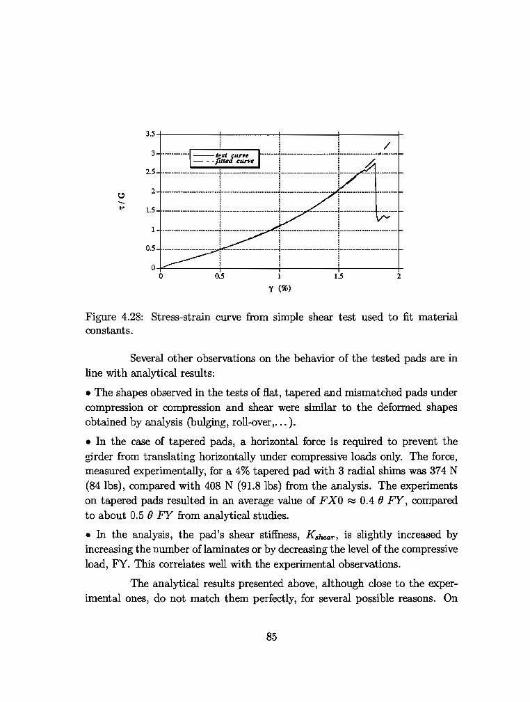
3.5+------!-----!-----+------+­/

3 ............... ::-::-: 1,:/eJ"[;:~e ········ j ·--···················--r·--···~· .. ···-···

2: =::=-+=+-~l=-=:::= ! ~ I

1.5 ············-················-r--·---·····-·····-·-r-········ ···············1············-··- -·······-~ ~ a

1 ...................................... .J. .............. _ ............. _.... -~: _ ................................................. -e .... ----................................. - .. : : :

~ ~ ~ 0.5 .............................. ·······-····~·-·········,································i ·····················-·····

0~---~----~----~-----+-0 0.5 1 1.5 2

'Y (%)

Figure 4.28: Stress-strain curve from simple shear test used to fit material constants.

Several other observations on the behavior of the tested pads are in line with analytical results:

• The shapes observed in the tests of flat, tapered and mismatched pads under compression or compression and shear were similar to the deformed shapes obtained by analysis (bulging, roll-over, ... ).

• In the case of tapered pads, a horizontal force is required to prevent the girder from translating horizontally under compressive loads only. The force, measured experimentally, for a 4% tapered pad with 3 radial shims was 374 N (84 lbs), compared with 408 N (91.8 lbs) from the analysis. The experiments on tapered pads resulted in an average value of FXO ~ 0.4 8 FY, compared to about 0.5 8 FY from analytical studies.

• In the analysis, the pad's shear stiffness, Kshear, is slightly increased by increasing the number of laminates or by decreasing the level of the compressive load, FY. This correlates well with the experimental observations.

The analytical results presented above, although close to the exper­imental ones, do not match them perfectly, for several possible reasons. On

85

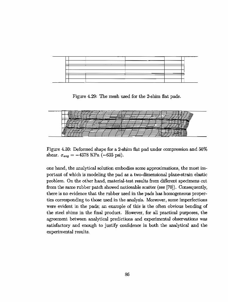
Figure 4.29: The mesh used for the 2-shim flat pads.

Figure 4.30: Deformed shape for a 2-shim flat pad under compression and 50% shear. O'avg = -4378 KPa ( -635 psi).

one hand, the analytical solution embodies some approximations, the most im­portant of which is modeling the pad as a two-dimensional plane-strain elastic problem. On the other hand, material-test results from different specimens cut from the same rubber patch showed noticeable scatter (see [70]). Consequently, there is no evidence that the rubber used in the pads has homogeneous proper­ties corresponding to those used in the analysis. Moreover, some imperfections were evident in the pads; an example of this is the often obvious bending of the steel shims in the final product. However, for all practical purposes, the agreement between analytical predictions and experimental observations was satisfactory and enough to justify confidence in both the analytical and the experimental results.

86

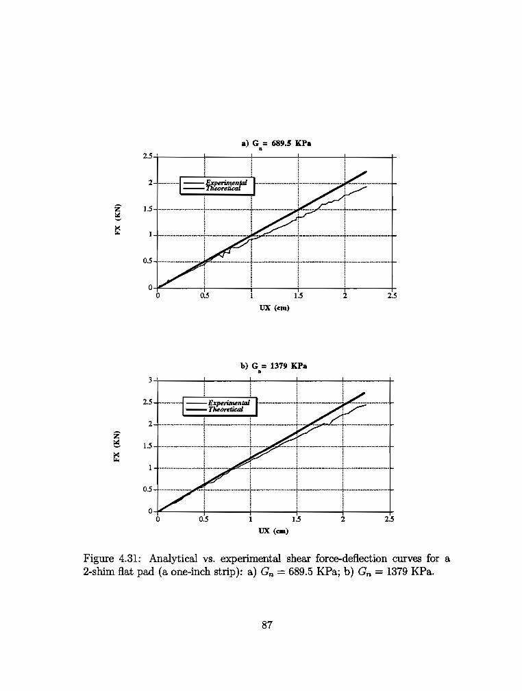
a) G = 689.5 KPa ll

2.5+----+----!-------J.----1-----+

2 -··i=;~:=t" ;t-·--t-·-- i -·-laS i : : : ............ _ ............. _ ...... ~~~---······--~--·---....... _r_·-----··--···· = ........... _ ............... T ........ ~ ........................... ..

~ ~ i : : : : : . : -··--··--··········1········--·---· ... . ................. _ ~ -······--··········1"""" ................................... .. ~ i E

o.s ........................ : -··················· j ·--····--·t··········--··········t-·····--·············

~ E ! 0~---r---~'r----+'----r' ----r

0 0.5 1.5 2 k5

UX (elll)

b) G = 1379 KPa ll

3+----~--~----+---~----+ i

k5 ···-···-i ~ Jjt!:~uu: 1····-···--··--r----... ··-.......... ; 2 ·········---·- 1--················j·----··-----+···· ... ·-t·-······-··········-·

~ ~ : ~ 1.5 ·····--··--··· ... ··-:···················-··!"········ · ·········r--· ... ···············-:·······-····-········

1 ........................ 1............. . ..... ; ........ ·---·--···f·····-·········---f···-···················· : ! ! !

··:·-··· ............... ~ •• u .......... r .............. ~ ...................... u .... r····-······--···· ..... .,. ................... _ ..................... .. 0.5

i ! I i 0~---r---~-----+-----~----+

0 0.5 l.S 2 2.5

UX (ea)

Figure 4.31: Analytical vs. experimental shear force-deflection curves for a 2-shim flat pad (a one-inch strip): a) Gn = 689.5 KPa; b) Gn = 1379 KPa.

87

Chapter 5

A MODEL FOR THE "WALKING" OF THE PAD

5.1 Introduction

Bridge bearing pads are held in place by friction with the abutment and the girders. However, in several cases pads have been observed to grad­ually and slowly move from their original position. This slip may continue to accumulate (over weeks or even months) and the pad may eventually fail to perform as designed. This phenomenon is referred to as "walking'' of the pad. It is believed that the walking problem is linked to the presence of the waxy substance added to the rubber as an ozone protector. The wax is believed to act as a lubricant when exuded to the surfaces of the pad.

Pad walking has sometimes been observed before the bridge was opened to traffic. This means that despite the absence of live loads due to vehicles, the pad may walk due to the movements and loads of the upper struc­ture of the bridge itself. Moreover, pads have walked in cases where the shear force due to the movement of the girders did not exceed the interface frictional capacity (normal load x coefficient of friction).

In this chapter, friction of elastomers is reviewed and the various factors affecting it are discussed. The hysteresis component of friction, which is the dominant component in lubricated surfaces, is emphasized. This leads to a regularized Coulomb friction law which is implemented in a model for the walking of the pad. The law introduces viscosity on the pad-girder and the pad-abutment interfaces. A simple model of the girder-pad-abutment system is described and examples are presented. The factors affecting walking are discussed.

88

5.2 Review of Rubber Friction

Early work on friction is attributed to well-known scientists: Leonardo da Vinci in late fifteenth century; Amontons in late sixteenth century; Coulomb in the eighteenth century; and Euler, also in the eighteenth century, who intro­duced the term "coefficient of friction" [72, 73, 74, 62]. The basic principles of friction put forward during that period can be summarized as follows:

• The coefficient of friction, p,, is a function of the materials of the contact­ing bodies.

• The static coefficient of friction, /lstatic, is higher than the dynamic coef­ficient of friction, /ldyna,mic, which is not a function of velocity, v.

• p, is neither a function of the normal load, N, nor a function of the contact area, A.

• Maximum frictional force = p, x N.

In late nineteenth century and early in the twentieth century, interest in friction was revived. Recent theories have categorized friction into different types depending on the lubrication [72, 73, 74]. These types, in the order of decreasing p,, are:

1. Dry Friction. No lubricant exists.

2. Boundary Friction. The lubricant film is very thin and interrupted by areas of solid contact.

3. Elasto-Hydrodynamic Friction. The lubricant film is thin but complete with no gaps. Friction force is transferred through the lubricant and through deformation of the bodies in contact.

4. Hydrodynamic Friction. Enough lubricant exists to warrant the use of fluid-mechanics equations (Reynold's equation) to solve the lubrication and friction problem. Types 3 and 4 are usually encountered between moving mechanical parts.

89

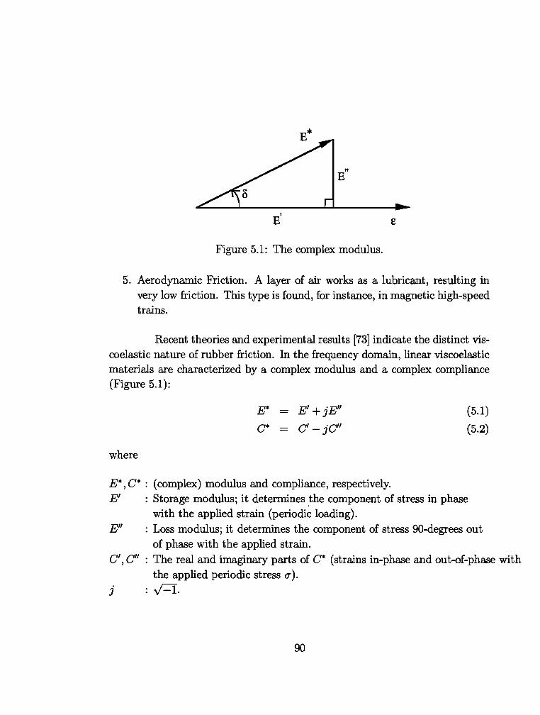
" E

I

E £

Figure 5.1: The complex modulus.

5. Aerodynamic Friction. A layer of air works as a lubricant, resulting in very low friction. This type is found, for instance, in magnetic high-speed trains.

Recent theories and experimental results [73] indicate the distinct vis­coelastic nature of rubber friction. In the frequency domain, linear viscoelastic materials are characterized by a complex modulus and a complex compliance (Figure 5.1):

where

E*

C*

E' + jE"

C'- jC"

E*, C* : (complex) modulus and compliance, respectively.

(5.1)

(5.2)

E' : Storage modulus; it determines ,the component of stress in phase with the applied strain (periodic loading).

E" : Loss modulus; it determines the component of stress 90-degrees out of phase with the applied strain.

C', C" : The real and imaginary parts of C* (strains in-phase and out-of-phase with the applied periodic stress u).

j :..;=I.

90

The loss tangent, tan 8, is defined as:

E" C" tan8 = E' = C' (5.3)

In general, tan 8 is a function of the frequency of the applied load, and is a measure of damping in the rubber. A highly dissipative rubber is characterized by a high loss tangent.

The friction force of the type encountered with bridge pads can be decomposed into two components, adhesion and hysteresis [73, 74, 75]:

(5.4)

hence: (5.5)

Adhesion:

This component is due to bond forces that develop between the molecules of the two contacting bodies. These forces arise at the real contact area and increase by the increase of this area. Therefore, adhesion is higher in smoother contact surfaces. Adhesion exists even as a component of static friction. In dynamic cases, however, another mechanism comes into the picture. Rubber chains that have formed links with the other surface are stretched until they rupture and release their energy. At the same time other links are being formed so that this process is repeated.

Different theories attempt to quantify adhesion friction. One such theory concludes a relationship of the form [73, 74]:

E' K1-tan8

'[I'

where Kt and rare constants, and pis the pressure (p = N fA).

Hysteresis:

(5.6)

This component is the sum of all forces needed to deform one body (rubber in this case) by the asperities of the other. In metal friction, this

91

component is associated with plastic deformations and breaking of the material at the asperity level, hence known as the "plowing friction." In general, this component is referred to as the deformation friction, and exists only when the relative tangential velocity, vr, between the two bodies is non-zero. For perfectly smooth surfaces, this force vanishes.

In !"ubber friction, the hysteresis component can be explained as fol­lows (Figure 5.2). Let the rubber be moving on top of a rigid surface with asperities. If VT is zero, the pressure that the asperity exerts on the rubber has a symmetric distribution around the asperity tip, and the net horizontal force is, therefore, zero. If VT, however, is not zero, the pressure distribution is skewed and a net horizontal resultant force is developed at each asperity tip. The sum of all of these individual forces comprise the hysteresis friction force. As vr increases, the pressure distribution is increasingly skewed, and Fhys increases. For high velocities, however, the rubber does not have enough time to conform to the asperities (Figure 5.2) and it touches only their tips. In this case, Fhys starts to decline again.

The nonsymmetric pressure distribution around the asperity is due to the delayed reaction of the rubber when deformed by the asperity. This causes its accumulation on the forward surface of the asperity facing the moving rubber. Thus, the material properties of the rubber are important factors in determining Fhys.

A theory for hysteresis friction, similar to the one for adhesion, results in the formula [73, 74]:

P,hys = K2 (;,) n tan8 (5.7)

where K 2 and n (> 1) are constants. Since it is the main component on lubricated surfaces, hysteresis is revisited in the next section.

Elements on the surface of the rubber are subjected to periodic load­ing from moving asperities. This, in addition to the repeated pattern of forming and rupturing adhesive bonds, implies cyclic storing, releasing, and losing en­ergy from the rubber. This process is very much dependent on the viscoelastic properties of the rubber. For this reason, tan8 appears in Equations (5.6) and (5.7).

92

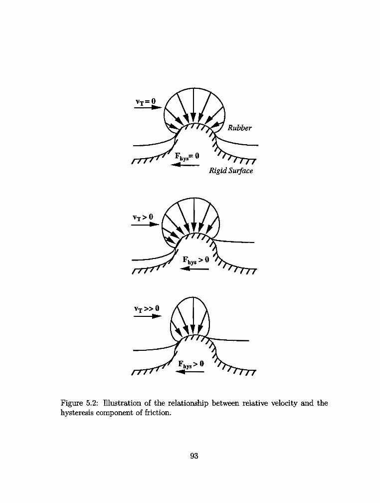
Rigid Surface

Figure 5.2: lllustration of the relationship between relative velocity and the hysteresis component of friction.

93

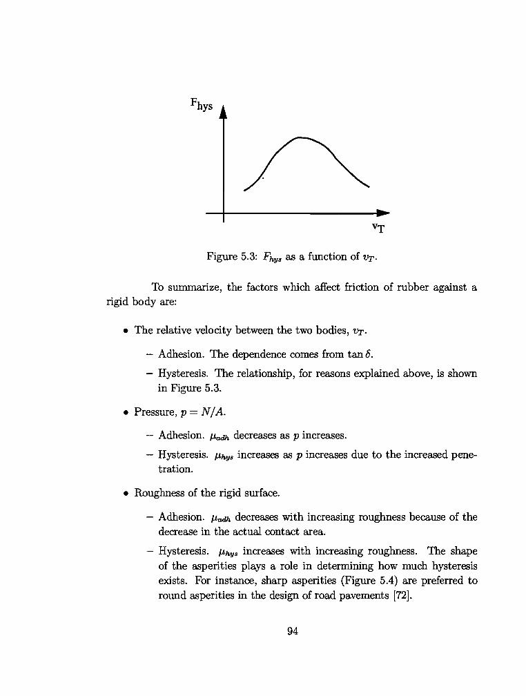
Figure 5.3: Fhys as a function of VT·

To summarize, the factors which affect friction of rubber against a rigid body are:

• The relative velocity between the two bodies, VT.

- Adhesion. The dependence comes from tan 8.

- Hysteresis. The relationship, for reasons explained above, is shown in Figure 5.3.

• Pressure, p = N /A.

- Adhesion. f..Ladh decreases asp increases.

- Hysteresis. f..Lhys increases asp increases due to the increased pene-tration.

• Roughness of the rigid surface.

- Adhesion. f..Ladh decreases with increasing roughness because of the decrease in the actual contact area.

- Hysteresis. f..Lhys increases with increasing roughness. The shape of the asperities plays a role in determining how much hysteresis exists. For instance, sharp asperities (Figure 5.4) are preferred to round asperities in the design of road pavements [72].

94

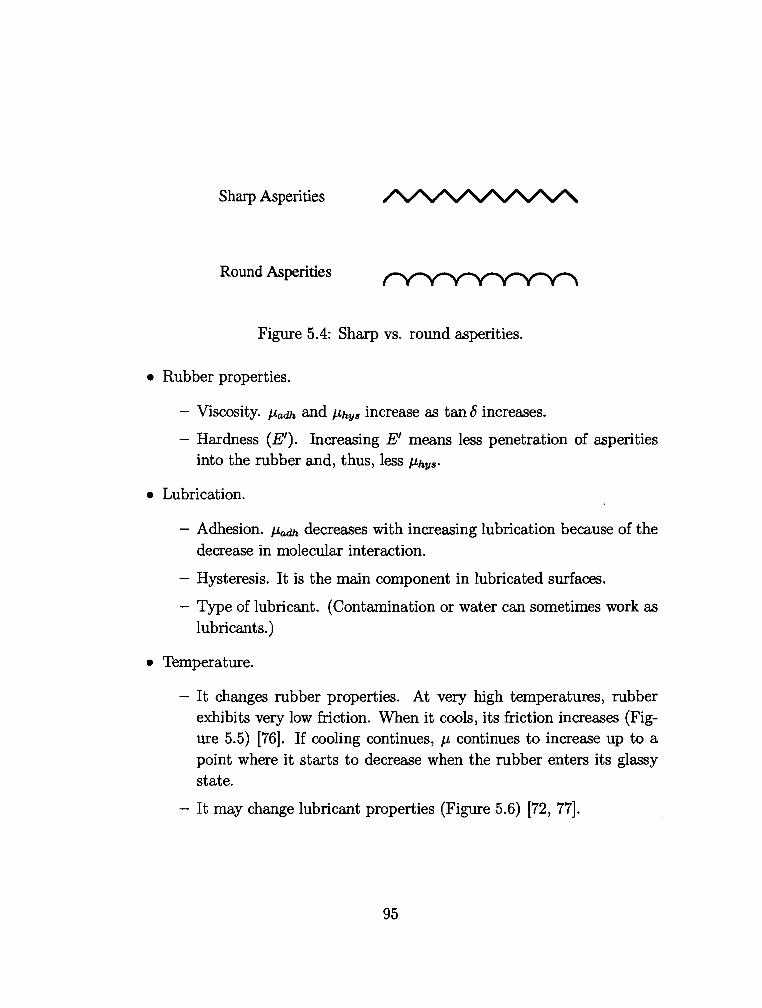
Sharp Asperities

Round Asperities

Figure 5.4: Sharp vs. round asperities.

• Rubber properties.

- Viscosity. f.ladh and J.lhys increase as tan 6 increases.

- Hardness (E'). Increasing E' means less penetration of asperities into the rubber and, thus, less f.lhys·

• Lubrication.

- Adhesion. J.ladh decreases with increasing lubrication because of the decrease in molecular interaction.

- Hysteresis. It is the main component in lubricated surfaces.

- Type of lubricant. (Contamination or water can sometimes work as lubricants.)

• Temperature.

- It changes rubber properties. At very high temperatures, rubber exhibits very low friction. When it cools, its friction increases (Fig­ure 5.5) [76]. If cooling continues, f.l continues to increase up to a point where it starts to decrease when the rubber enters its glassy state.

- It may change lubricant properties (Figure 5.6) {72, 77].

95

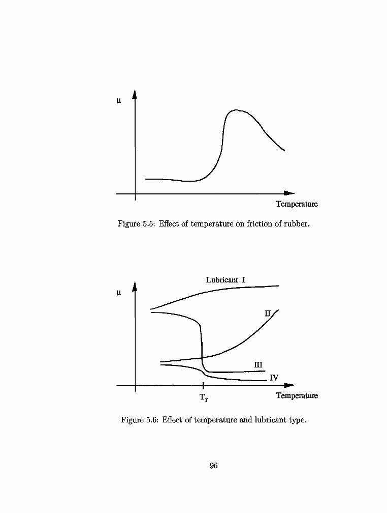
Temperature

Figure 5.5: Effect of temperature on friction of rubber.

Lubricant I

!l

Temperature

Figure 5.6: Effect of temperature and lubricant type.

96

With regard to friction of bearing pads, the coefficient of dry friction was discussed in a paper by Schrage [13]. Quantitatively, a relationship was presented for J.L as a function of p. It is of the form:

/3 J.L=a+- ~~

p

This form of J.L is similar to the apparent coefficient of friction in granular materials (such as sands) that exhibit cohesion and friction [78]:

s /3 s = /3 + ap * J.L = - = a + - (5.9) p p

where s is the shear strength of the soil and a and /3 are the coefficient of friction and the cohesion of the soil, respectively. Comparing Equation ( 5.8) to Equations ( 5.6) and (5.7) shows that the form of relationship ( 5.8) (specifically the dependence on pressure) is not very accurate.

In other related work [79, 11, 12, 4], the "walking'' problem has been attributed to shear forces which exceed the friction capacity of the interfaces. Viscosity-induced slipping, however, has not been mentioned in any literature. The solution introduced and adopted by the current AASHTO specification [80] is to limit the maximum shear force to one-fifth of the minimum compressive force. If that limit is not met, the pad is required to be restrained.

5.3 The Hysteresis Component

The theory outlined here is called the unified theory [73, 7 4] since a similar theory is used to arrive at an expression for the adhesion component. Fhys is the sum of hysteresis forces at all asperity tips in contact with the rubber. Each of these individual forces equals the energy dissipated by the volume of rubber deformed and displaced by the asperity, divided by the distance between neighboring asperities.

Specific geometries for the rigid surface are assumed and the energies lost are expressed as the product of the loss modulus, E", by the volume of the deformed rubber. Using solutions for these volumes from elasticity theory, one finally arrives at an expression of the form:

J.Lhys = 4 C "( (~)n tan6 (5.10)

97

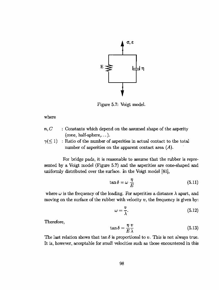
0', £

E

Figure 5.7: Voigt model.

where

n, C : Constants which depend on the assumed shape of the asperity (.cone, half-sphere, ... ).

1( < 1) : Ratio of the number of asperities in actual contact to the total number of asperities on the apparent contact area (A).

For bridge pads, it is reasonable to assume that the rubber is repre­sented by a Voigt model (Figure 5. 7) and the asperities are cone-shaped and uniformly distributed over the surface. In the Voigt model [81],

tan6 =w; (5.11)

where w is the frequency of the loading. For asperities a distance .>t apart, and moving on the surface of the rubber with velocity v, the frequency is given by:

Therefore, 1JV

tan6 = -­E.>t

(5.12)

(5.13)

The last relation shows that tan 6 is proportional to v. This is not always true. It is, however, acceptable for small velocities such as those encountered in this

98

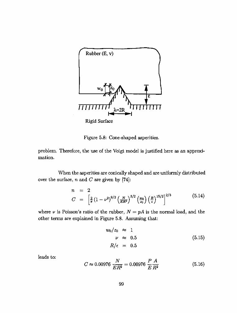
Rubber (E, v)

Rigid Surface

Figure 5.8: Cone-shaped asperities.

problem. Therefore, the use of the Voigt model is justified here as an approxi­mation.

When the asperities are conically shaped and are uniformly distributed over the surface, nand Care given by [74]:

n 2

c = [~<1 -v2>9/2 (-lfrr)3'2 (::;:) (~f5/2r'3 (5.14)

where vis Poisson's ratio of the rubber, N =pAis the normal load, and the other terms are explained in Figure 5.8. Assuming that:

wo/Zo ~ 1

l/ ~ 0.5 (5.15)

R/E - 0.5

leads to: N PA

C ~ 0.00976 ER2 = 0.00976 E R 2 (5.16}

99

In the case of cone-shaped asperities:

>.. = 2R (5.17)

Substituting back into Equation ( 5.10) yields:

A TJ (P)s /.Lhys = 0.02 R3 E E v (5.18)

where 1 has been assumed to be 1 (i.e., all asperities are in contact), a reason­able assumption for quasi-static problems.

On the basis of the above equation, the following observations can be made:

1. /.Lhys is proportional to v.

2. As R increases (fewer, bigger asperities), /.Lhys decreases.

3. /.Lhys is proportional to the ratio P / E (J.Lhys is lower for harder rubbers).

4. TJ/ E in the Voigt model is called the retardation time. It is on the order of the time needed for creep to complete. As this time increases, /.Lhys

increases.

5.4 Regularized Coulomb Friction

Coulomb's law of friction, extended for the dynamic case (Figure 5.9), states that the friction force between two bodies moving relative to each other does not depend on the velocity. It is, however, proportional to the normal force applied at the interface:

(5.19)

where

F1 : The friction force. J.L : Proportionality factor = Coefficient of friction. N : The normal load.

100

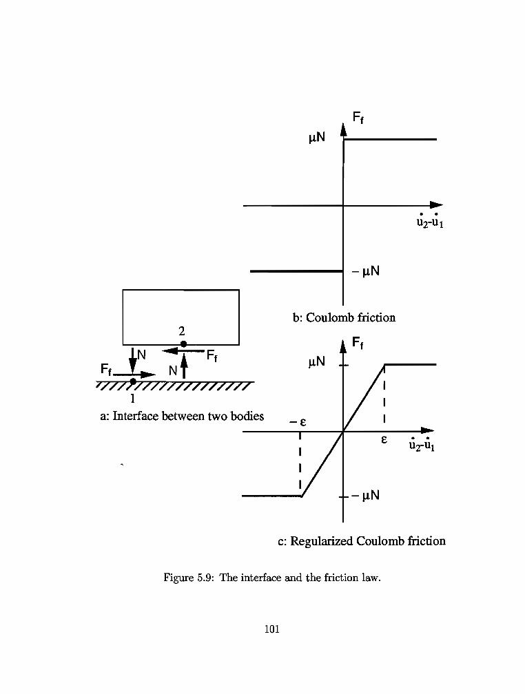
------t -J.lN

2

F,L :t F, 777/h7777777777777

1

a: Interface between two bodies

b: Coulomb friction

• •

• •

c: Regularized Coulomb friction

Figure 5.9: The interface and the friction law.

101

Coulomb's law is modified (regularized) so that the friction force is a linear function of relative velocity in the range -e < (ii2 - iii)< e, where

ii2 - ii1 : Difference in tangential ( i.e., in the direction of the tangent of the interface) velocities of contacting bodies 1 and 2.

e : Regularization parameter.

The regularization serves two purposes. First, it removes the discontinuity in the neighborhood of zero relative tangential velocity. Second, with the velocity­dependent linear part, the model now more accurately represents the physical phenomenon of friction discussed earlier. Since the problem of the pad is a quasistatic one, the analysis is mostly over that linear part.

Over the linear region, the friction force is proportional to the normal force Nand the ratio(~- ii1)/e. As shown in Figure 5.9, the friction force in regularized Coulomb friction law is given by:

{

p, u2~'"1 N - e < (ii2- ii1) < e, Ft=

11. u2- 1h N otherwise. ,.., lu2-u1l

(5.20)

The velocity-dependent linear part introduces viscous effects into the frictional model. It is clear from Equation ( 5.20) that increasing the parameter e reduces the friction force F1 and widens the range over which viscous behavior prevails. Therefore, e is referred to as a viscosity parameter.

To get some physical insight and qualitative feeling of the viscos­ity parameter, e, the friction force F1 (Equation ( 5.20)) is compared to the hysteresis-friction force (Equation ( 5.18)) yielding :

j.t = /-thys = 0.02 ~ !]_ (1!..) 3 e v R3 E E

(5.21)

The last equation indicates that, besides being a function of the viscous prop­erties of the elastomer ( 11/ E), e is a function of the properties of the surface it is rubbing against (its microtexture). In addition, on lubricated interfaces, e is a function of the ratio pf E. In conclusion, increasing the hysteresis component, the primary component of friction on lubricated surfaces, requires a smaller e.

102

5.5 Modeling the Pad

At each girder end, three separate bodies interact: the girder, the pad, and the abutment. The vertical load of the girder is transferred to the abutment through the pad. In addition, the pad by its shear flexibility accommodates the horizontal translations of the girder end due to thermal as well as other effects (concrete shrinkage, creep, etc.).

The girder and the abutment apply two types of stresses on the sur­faces of the pad: normal and tangential. In the model used, the stresses are replaced by resultant forces (normal and tangential) at nodal points located along the interfaces (Figure 5.10).

A tapered pad is used to accommodate a girder with inclination of an angle () relative to the abutment. A dynamic model is developed to facilitate the incorporation of both the velocity-dependent friction law introduced above and the time-dependent quantities such as displacements, loads, etc. Nodes 0 and 1 are located on the abutment and on the bottom of the pad, respectively, to monitor the motion at that interface. Similarly, two nodes, 2 and g, are placed on the top of the pad and on the girder, respectively. Usually Node 0 is motionless and the vertical load and horizontal movement of Node g are prescribed. The pad, the nodes, and the set of forces acting on the interfaces are shown in Figure 5.10.

Two coordinate systems are defined, (x, y) and (x', y') (Figure 5.10). A transformation matrix is used to relate quantities relative to the level system (x,y) to quantities relative to the inclined system (x',y'):

{ u~} [cosO sin()]{Ua} v~ - -sinO cosO v2

where

u, v : Displacements in the x and y-directions, respectively. u', v': Displacements in the x' and y' -directions, respectively.

The quantities involved in the model are as follows:

103

(5.22)

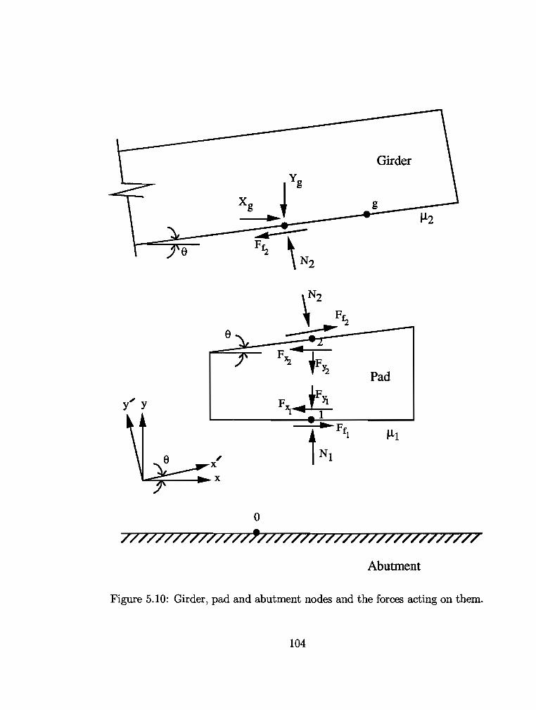
Girder

Xg i Yg g

.... Jl2

a \N2 \N2

Ftz

a ~

F .... ~ "l F~

Pad

y' y F~ "1 1 .... Fe

Jll tNt I , X

X

0

777777777777777177777777777777777777777777

Abutment

Figure 5.10: Girder, pad and abutment nodes and the forces acting on them.

104

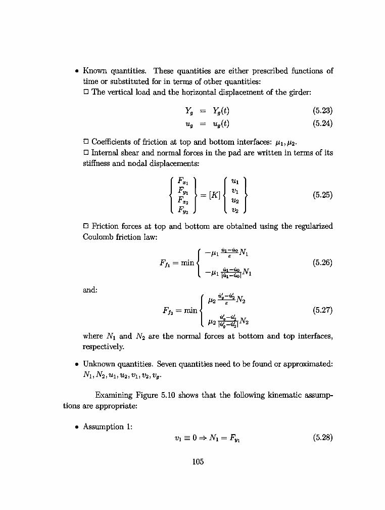
• Known quantities. These quantities are either prescribed functions of time or substituted for in terms of other quantities: 0 The vertical load and the horizontal displacement of the girder:

Yg - Yg(t)

Ug u9 (t)

0 Coefficients of friction at top and bottom interfaces: J.lb J.t2 •

(5.23)

(5.24)

0 Internal shear and normal forces in the pad are written in terms of its stiffness and nodal displacements:

(5.25)

0 Friction forces at top and bottom are obtained using the regularized Coulomb friction law:

and:

Fh =min {

~N J.l2 g 2

il-~ J.l2~N2

(5.26)

(5.27)

where N1 and N2 are the normal forces at bottom and top interfaces, respectively.

• Unknown quantities. Seven quantities need to be found or approximated: N1 , N2 , u 1 , u2 , v1 , v2 , v9 •

Examining Figure 5.10 shows that the following kinematic assump­tions are appropriate:

• Assumption 1: (5.28)

105

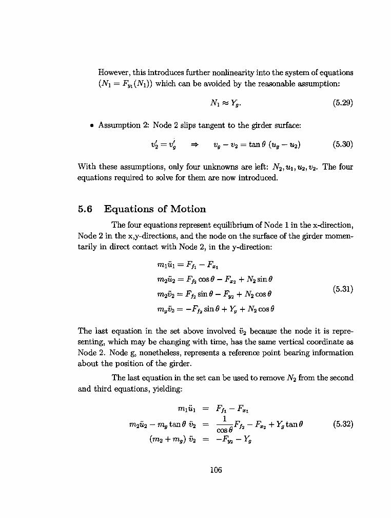
However, this introduces further nonlinearity into the system of equations (NI = Fy1 (NI)) which can be avoided by the reasonable assumption:

(5.29)

• Assumption 2: Node 2 slips tangent to the girder surface:

(5.30)

With these assumptions, only four unknowns are left: N2, Ut, u2, v2. The four equations required to solve for them are now introduced.

5.6 Equations of Motion

The four equations represent equilibrium of Node 1 in the x-direction, Node 2 in the x,y-directions, and the node on the surface of the girder momen­tarily in direct contact with Node 2, in they-direction:

m1ii1 = F11- Fx1

ffl2ii2 = F12 cos 0 - Fx2 + N2 sin 0

ffl2V2 = F12 sin 0 - Fy2 + N2 cos 0

m9 ii2 = -Fh sin 0 + Yy + N2 cos 0

(5.31)

The last equation in the set above involved ii2 because the node it is repre­senting, which may be changing with time, has the same vertical coordinate as Node 2. Node g, nonetheless, represents a reference point bearing information about the position of the girder.

The last equation in the set can be used to remove N 2 from the second and third equations, yielding:

m2ii2 - m9 tan 0 ii2

(m2 + m9 ) ii2

106

(5.32)

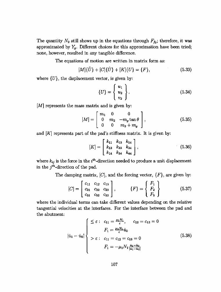
The quantity N2 still shows up in the equations through F12 ; therefore, it was approximated by Yg. Different choices for this approximation have been tried; none, however, resulted in any tangible difference.

The equations of motion are written in matrix form as:

[M){U} + [C]{ir} + [K]{U} = {F}, {5.33)

where { U}, the displacement vector, is given by:

(5.34)

[M] represents the mass matrix and is given by:

[M] [ ~1 ~2 -m9°tane] , o 0 ma+m9

{5.35)

and [K] represents part of the pad's stiffness matrix. It is given by:

[K] = [ ~~~ ~~: ~~ l ' k14 ks4 k44

. {5.36)

where kii is the force in the ith-direction needed to produce a unit displacement in the lh-direction of the pad.

The damping matrix, [C], and the forcing vector, {F}, are given by:

[

Cn C12 C13] [C] = C21 C22 C23 ,

C31 C32 Cgg

{5.37)

where the individual terms can take different values depending on the relative tangential velocities at the interfaces. For the interface between the pad and the abutment:

< c •• c11 -- e1!:'1 , c c - 0 v c 12 = 13-

F1 e1;r1 uo

> e : Cn C12 C13 = 0 (5.38)

F =-II N 'li.1-'li.Q 1 ,-l 1 lu1 -'li.ol

107

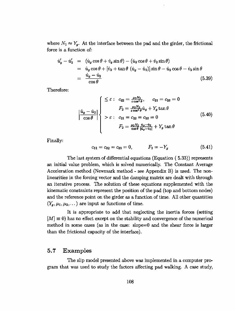
where N 1 ~ Yg. At the interface between the pad and the girder, the frictional force is a function of:

(u9 cos 0 + v9 sinO)- (u2 cos 0 + v2 sinO)

u9 cos 0 + [v2 + tanO (u9 - u2)] sinO- u2 cos 0- v2 sinO

Therefore:

Finally:

u9 -u2

cosO

l

u9 - iL21 cosO

< e : r~ _ P.2N2. ~~~ - eco528' ~1 = ~3 = 0

F2 = e~~28 u9 + Yg tanO

> e : C21 = C22 = C23 = 0

F2 = JI.2N82I~u-~l + Yg tanO COS Ug-U2

C31 = C32 = C33 = 0, Fg = -Yg

(5.39)

(5.40)

(5.41)

The last system of differential equations (Equation ( 5.33)) represents an initial value problem, which is solved numerically. The Constant Average Acceleration method (Newmark method- see Appendix B) is used. The non­linearities in the forcing vector and the damping matrix are dealt with through an iterative process. The solution of these equations supplemented with the kinematic constraints represent the position of the pad (top and bottom nodes) and the reference point on the girder as a function of time. All other quantities (Yg, /1-1, /1-2, ... ) are input as functions of time.

It is appropriate to add that neglecting the inertia forces (setting [M] = 0) has no effect except on the stability and convergence of the numerical method in some cases (as in the case: slope=O and the shear force is larger than the frictional capacity of the interface).

5. 7 Examples

The slip model presented above was implemented in a computer pr<r gram that was used to study the factors affecting pad walking. A case study,

108

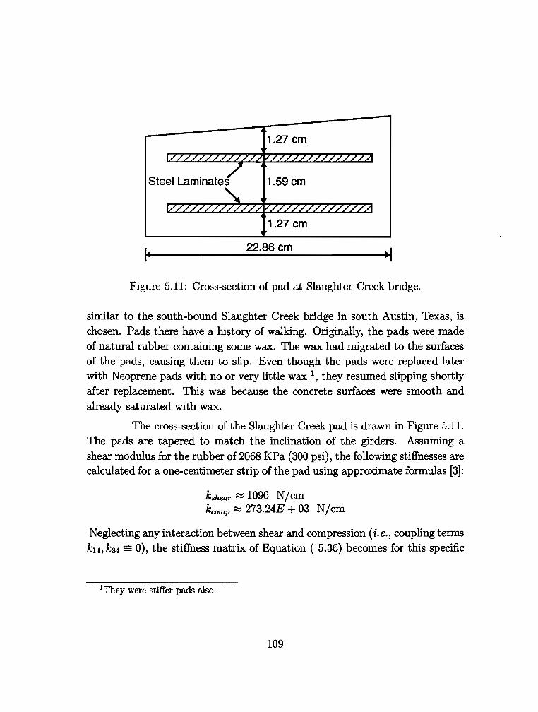
22.86 em

Figure 5.11: Cross-section of pad at Slaughter Creek bridge.

similar to the south-bound Slaughter Creek bridge in south Austin, Texas, is chosen. Pads there have a history of walking. Originally, the pads were made of natural rubber containing some wax. The wax had migrated to the surfaces of the pads, causing them to slip. Even though the pads were replaced later with Neoprene pads with no or very little wax 1, they resumed slipping shortly after replacement. This was because the concrete surfaces were smooth and already saturated with wax.

The cross-section of the Slaughter Creek pad is drawn in Figure 5.11. The pads are tapered to match the inclination of the girders. Assuming a shear modulus for the rubber of 2068 KPa (300 psi), the following stiffnesses are calculated for a one-centimeter strip of the pad using approximate formulas [3]:

kshear ~ 1096 N I em kcomp ~ 273.24E + 03 N /em

Neglecting any interaction between shear and compression (i.e., coupling terms k14, k34 = 0), the stiffness matrix of Equation ( 5.36) becomes for this specific

1They were stiffer pads also.

109

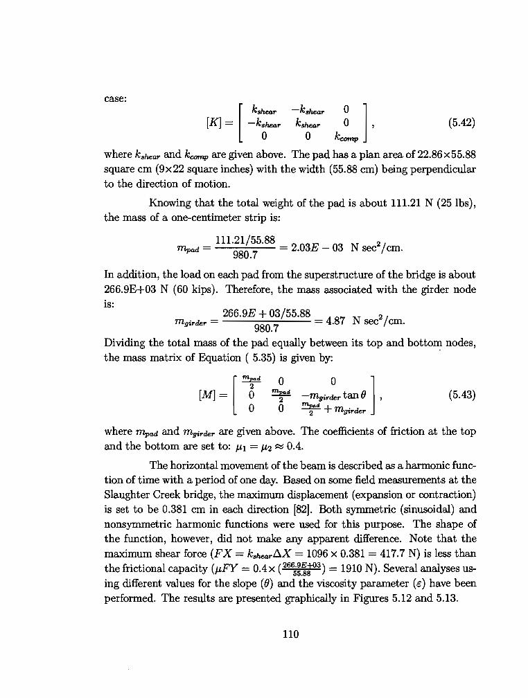
case:

[K] [

ks~u:ar -kshear

-kshear kshear

0 0 ~ l ' kCO'Inp

(5.42)

where kshear and kCO'Inp are given above. The pad has a plan area of 22.86x55.88 square em {9x22 square inches) with the width (55.88 em) being perpendicular to the direction of motion.

Knowing that the total weight of the pad is about 111.21 N (25 lbs), the mass of a one-centimeter strip is:

= 111.21/55.88 = 2 03E _ 03 N 2/ 11'lpad

980.7

. sec em.

In addition, the load on each pad from the superstructure of the bridge is about 266.9E+03 N (60 kips). Therefore, the mass associated with the girder node is:

mgirder 266.9E + 03/55.88 = 4 87 N 2 /

980.7 . sec em.

Dividing the total mass of the pad equally between its top and botto~ nodes, the mass matrix of Equation ( 5.35) is given by:

[M] = 5 m~od -mgirder tan() , [ ~ 0 0 l

0 0 mrd + mgirder

(5.43)

where 'mpa.d and mgirder are given above. The coefficients of friction at the top and the bottom are set to: J.LI = J.L2 ~ 0.4.

The horizontal movement of the beam is described as a harmonic func­tion of time with a period of one day. Based on some field measurements at the Slaughter Creek bridge, the maximum displacement (expansion or contraction) is set to be 0.381 em in each direction [82]. Both symmetric (sinusoidal) and nonsymmetric harmonic functions were used for this purpose. The shape of the function, however, did not make any apparent difference. Note that the maximum shear force (FX = kshearllX 1096 x 0.381 = 417.7 N) is less than the frictional capacity (J.LFY = 0.4x e665:~3 ) = 1910 N). Several analyses us­ing different values for the slope (0) and the viscosity parameter (e) have been performed. The results are presented graphically in Figures 5.12 and 5.13.

110

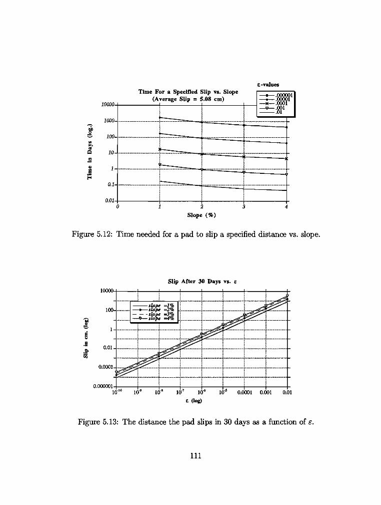
,-.. l:lil .s '-'

"' >.

" Q

.5! Gl

E E:

£-values

10000

1000

Time For a Specified Slip vs. Slope --w1 (Average Slip = 5.08 em) --+-. 1 ,_----------------~--------------------~----------------~----~~- 1 --v--__ :8?1

~ ·································F·········::::-:::::: ......... =-.... -t··=·········==·········==·········::f=··-·····=·········=·········=:J········

100 ~

································F~········::::::::: ........ ::::..-..... -t=········=········::::::::·········~······+:::::········=········=·········=f······

10

1

*-·······························~fr···===······=······=·····---,r=····=······=·····:::::::······::::·····~····-~·····=······=······=·····=······j···

································-Fr·=······===·········=·······-+=·····=·········:.:::::::········::4······+==·········==········=·········=±·····

0.1 i--································rr==······::::::::: ........ ::::..-..... -r=········=········===·········~······-:=········=········=·········==J······

0. 0 1,_-----------------i------------------+------------------i---------------------+-o 1 2

Slope (%)

3 4

Figure 5.12: Time needed for a pad to slip a specified distance vs. slope.

El .. .e .eo ~

Slip After 30 Days vs. £

10000,_------+-----~---------+---------r--------+---------~----~---------r

.--'----...... ----.. . . . . --slope =I% ·1···············-r··············r···············1···············:··;;;,

100 ::::= ~:~~ 3i i:=~l=r~~+=-+----------------·-t··-----------·-t··-------------~----------------:------ - - -----------··f··------------·t··-------------

: : ! ~ . ! : ---·············r····------·-··r··---------···-!··;· ~- ··= -------·-·-··r··············-~------·······-·T···············

001 : : ::;;oo:: : : : :

• ················r··············+····· ··· ·············j···············r··············r-·············r··············

0.0001 ::::::·:=·:::··:~·-······+:::::::::::::J:::::::::::::::I:::::::::::::r:::::::::::::r:::::::::::::J::::::::::::::: ------------·-I···············r····--------.. ··~·-··············f···············y·······--------~----·-----·----T····-----·-·---

o.oooooi ,_ ________ +' --------....,'f---+' ---------+-' ---------t'---------+' ---------;'r------+ 10·10 10-c; 0.0001 0.001 O.Ql

£ (Jog)

Figure 5.13: The distance the pad slips in 30 days as a function of c.

111

The first figure (Figure 5.12) shows the time (in days) needed for a pad with different values of e to walk an average of 5.08 em, versus the slope (8). The average slip is defined as the average of the horizontal displacements of the top and the bottom nodes (Nodes 1 and 2) of the pad. The graphs have not been extended to the zero value of slope since absolutely no walking occurs for this case; a perfectly flat pad will not have a net slip for symmetry reasons. In Figure 5.13, the average slip (in em) which takes place over a period of 30 days is plotted as a function of the parameter e for different values of the slope. It is clear from these graphs that increasing the slope and/or the viscosity parameter increases the slip of the pad. However, for very small values of e (dry, rough surfaces) or zero slopes, the slip is negligible.

For a qualitative study of the walking, the displacements vs. time of Node 1 and Node 2 of the pad and the prescribed motion of the girder (Node g) are shown for different cases in Figures 5.14 through 5.18. These graphs were chosen as samples to illustrate some characteristic behaviors.

Figures 5.14 and 5.15 correspond to a flat pad with two extreme values of w-s and w-a' respectively, given for the parameter e. Although, for a large value of e {I0-3), the top and the bottom of the pad slip back and forth (approximately half the distance the girder moves), no net walking is obtained when the slope vanishes.

The movements encountered in a tapered pad (slope= I%) for low (10-8), medium (5 X IQ-5) and high (2 X 10-4) values for c are plotted in Figures 5.16 to 5.18 as functions of time. When e is low, the top of the pad moves along with the girder, while its bottom sticks to the abutment with no overall walking over time. The pad in this case behaves as intended. For the medium-valued e, the (tapered) pad inches gradually out of place, as shown in Figure 5.17. For high e's, however, (very low friction) the top and the bottom of the pad move almost together; i.e., the pad is squeezed out as a rigid body.

In reality, a perfect zero slope is almost impossible to achieve. There­fore, practically every pad is prone to walk provided that slippery smooth interfaces exist. This conclusion agrees well with the field observations [71]. Pads in use have been observed to walk whenever a waxy substance has coated their surfaces, thus producing the viscous effects included in this simple model.

112

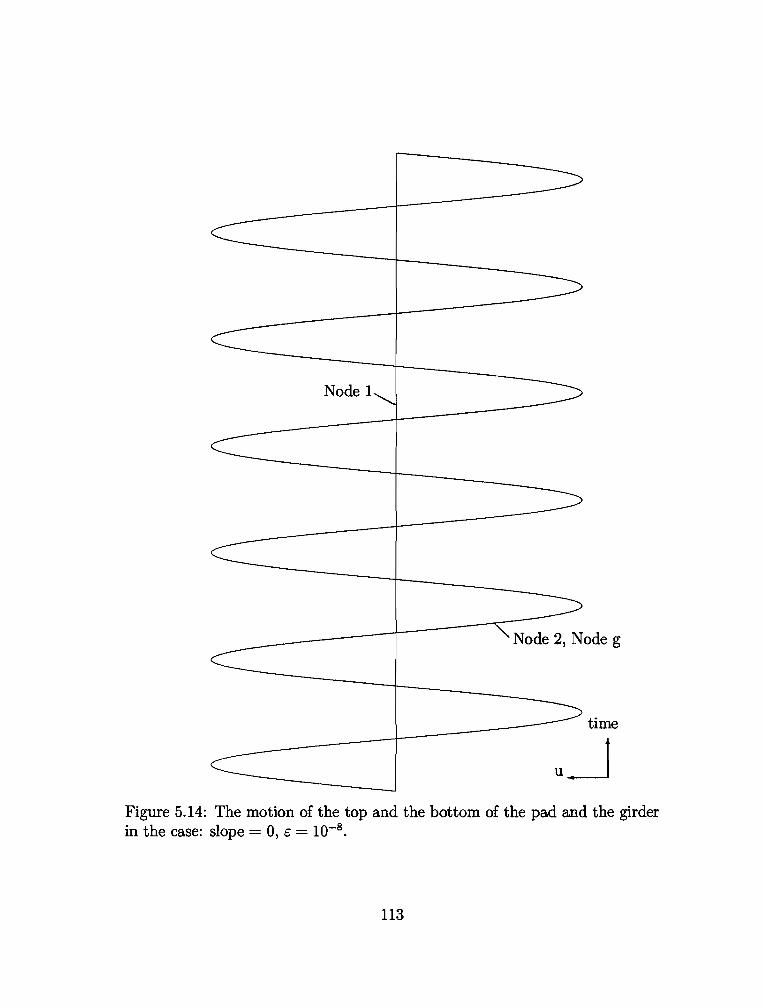
Node 1

time

Figure 5.14: The motion of the top and the bottom of the Pad Blld the girder

in the case: slope= 0, c = 10-8•

113

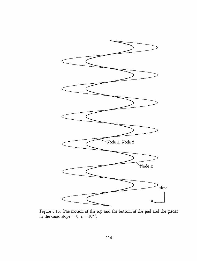
Node 1, Node 2

time

Figure 5.15: The motion of the top a.nd the bottom of the pad a.nd the @.rder in the case: slope ::::::. 0, e = 10-

3

.

114

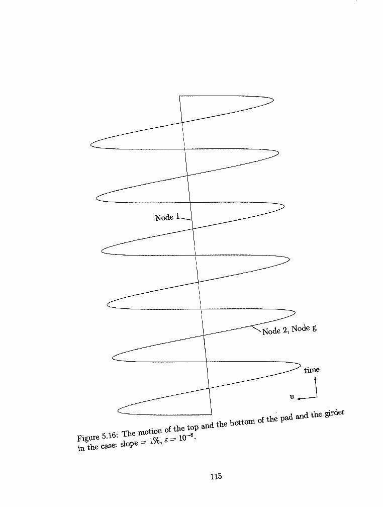
Node 1

time

FigUI<' 5.16: The motion of the toP and the bottom of the pad and the girdet

in the case: slope ::::: 1%, £ = 10-8

.

115

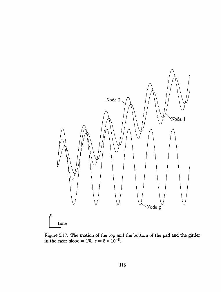
Nodeg

u

Gm· Figure 5.17: The motion of the top and the bottom of the pad and the girder in the case: slope = 1%, e = 5 X 10-5•

116

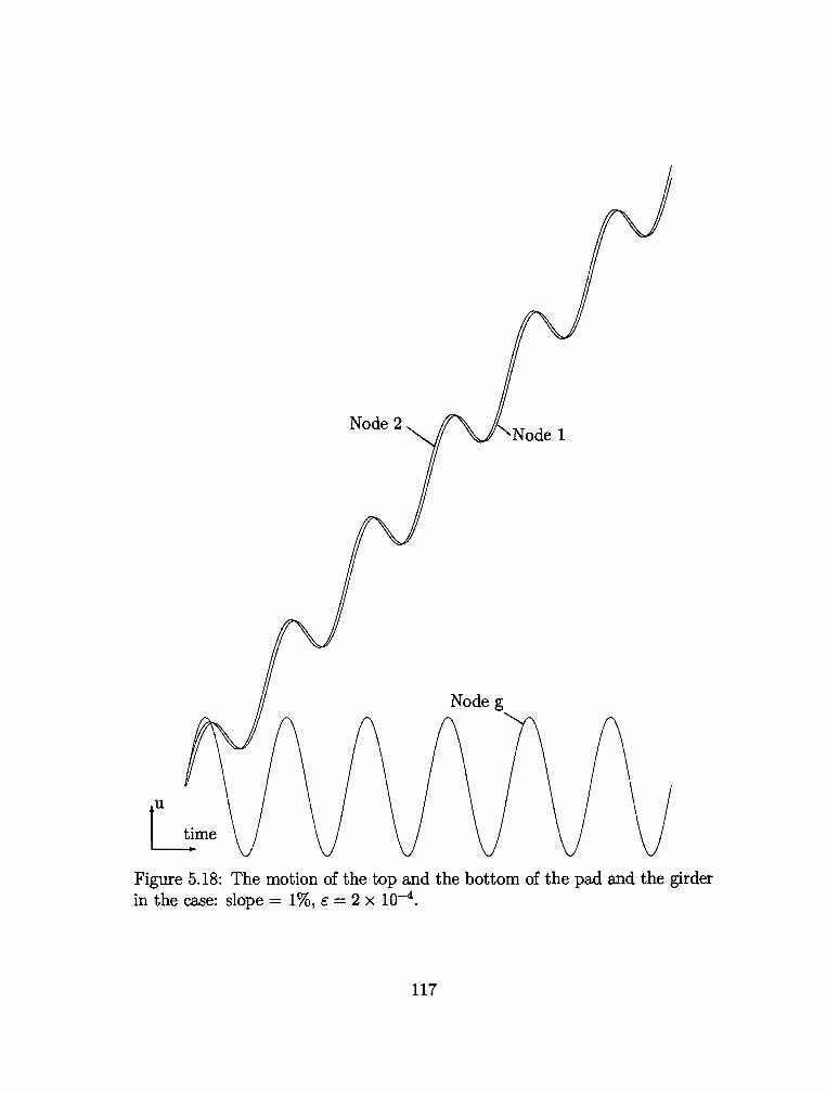
Nodeg

u

~me Figure 5.18: The motion of the top and the bottom of the pad and the girder in the case: slope = 1%, s = 2 x 10-4

•

117

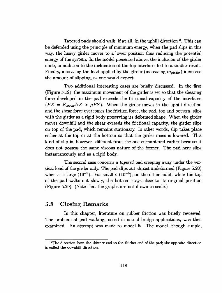
Tapered pads should walk, if at all, in the uphill direction 2 • This can be defended using the principle of minimum energy; when the pad slips in this way, the heavy girder moves to a lower position thus reducing the potential energy of the system. In the model presented above, the inclusion of the girder node, in addition to the inclination of the top interface, led to a similar result. Finally, increasing the load applied by the girder (increasing mgirder} increases the amount of slipping, as one would expect.

Two additional interesting cases are briefly discussed. In the first (Figure 5.19), the maximum movement of the girder is set so that the shearing force developed in the pad exceeds the frictional capacity of the interfaces (FX = Kshe.arD.X > p,FY}. When the girder moves in the uphill direction and the shear force overcomes the friction force, the pad, top and bottom, slips with the girder as a rigid body preserving its deformed shape. When the girder moves downhill and the shear exceeds the frictional capacity, the girder slips on top of the pad, which remains stationary. In other words, slip takes place either at the top or at the bottom so that the girder mass is lowered. This kind of slip is, however, different from the one encountered earlier because it does not possess the same viscous nature of the former. The pad here slips instantaneously and as a rigid body.

The second case concerns a tapered pad creeping away under the ver­tical load of the girder only. The pad slips out almost undeformed (Figure 5.20) when e. is large (lo-3). For small e. (lo-6), on the other hand, while the top of the pad walks out slowly, the bottom stays close to its original position (Figure 5.20}. (Note that the graphs are not drawn to scale.}

5.8 Closing Remarks

In this chapter, literature on rubber friction was briefly reviewed. The problem of pad walking, noted in actual bridge applications, was then examined. An attempt was made to model it. The model, though simple,

2The direction from the thinner end to the thicker end of the pad; the opposite direction is called the downhill direction.

118

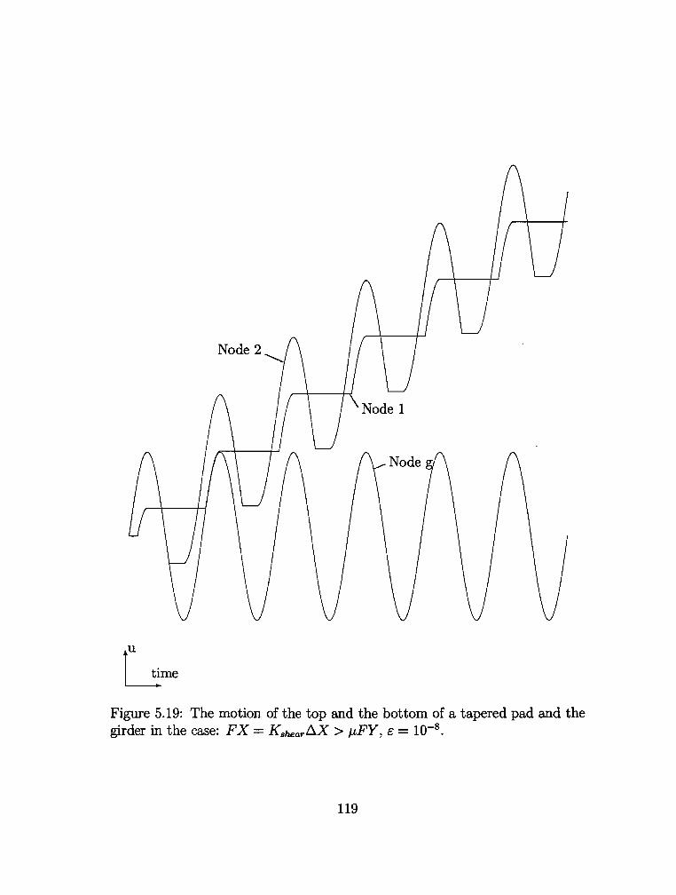
Figure 5.19: The motion of the top and the bottom of a tapered pad and the girder in the case: FX = Kshearf).X > J.LFY, € = 10-8

.

119

a)

b)

Node 2"\

\

Nodeg

Node 1

Nodeg

\ \

Figure 5.20: The motion of the top and the bottom of a tapered pad and the girder under the vertical load of the girder only: a) e = w-3 , b) e = w-6

•

120

was able to predict behavior similar to that found in the field studies. Large values of e, which are interpreted in the field as waxy smooth interfaces, are responsible for the walking of the pad even in cases where the available friction capacity has not been overcome.

Moreover, the use of this dynamic model facilitated the inclusion of time-dependent quantities and the incorporation of viscous friction. The model must be validated with lab tests, and its parameters should be calibrated. Further in-depth study for the parameter e is required.

Finally, when wax exists, the adhesion component of friction becomes minimal. The hysteresis component, which is not affected by the wax, remains as the only friction. As given by Equation ( 5.18), this component is a func­tion of the properties of the concrete surface and the viscous properties of the rubber. On smooth surfaces, the hysteresis component becomes very small. Smooth surfaces and wax are, therefore, a recipe for walking. In such cases, it is helpful to try to increase the hysteresis component although this would not guarantee eliminating the walking problem. Some ways to accomplish that are to use rough concrete surfaces (sharp asperities are preferred for this purpose) and to use softer elastomers (lower E).

121

Chapter 6

CONCLUSIONS AND RECOMMENDATIONS

In most cases, elastomeric bridge bearings have performed satisfacto­rily. Occasionally, however, they failed due to a variety of reasons; walking is the most-reported failure mode in the state of Texas. This work was an effort towards better understanding of the behavior of these pads that will contribute to the ultimate goal of perfecting their design and performance.

An analytical model for the structural analysis of elastomeric bear­ings was developed and implemented. The model involves a p-version nonlinear finite element method accompanied with a frictional-contact algorithm for the interaction with other bodies. Material as well as geometrical nonlinearities were included. Furthermore, points on the contact surface may stick1 slip or separate, thus modifying the limits of the real contact surface and adding more nonlinearities to the model. The penalty method was used in the contact algo­rithm, and Lagrange multipliers were used to enforce rubber incompressibility.

The element performed favorably in both theoretical examples and bearing applications. By allowing the choice of different orders of interpolation at different places, the method provides better control of the constraint count than the usual h-version method. Also, the p-version does not require any remeshing of the domain for higher p's. However, it is more difficult to specify some boundary conditions (curved edges for example) on the suggested element.

Using practical examples, the rule stating that the constraint count in two-dimensional discretized boundary value problems must be close to two, was shown to be valid for the higher-order element. The integration rule needed to integrate the finite element equations should have an order at least equal to that of the element.

While the compressive stiffness of an elastomeric bearing increases at large axial loads, its shear stiffness remains almost constant, with an apparent

122

shear modulus slightly less than that of the rubber itself. No signifigant effects on stiffnesses, stresses or strains were associated with tapered pads (up to · 4%). Keeping the total thickness of the elastomer the same, a pad with more steel laminates behaves better: whereas the compressive stiffness is noticeably increased, the shear flexibility is kept intact; stresses, strains and edge effects (bulging and roll-over) are significantly reduced.

Using elastomers with higher shear modulus produces stiffer pads with smaller strains. However, since the horizontal deflection of the bearing rather than the force is prescribed, some stresses may increase. If a slope mismatch (initial imperfection) between the pad and the girder exist, the pad's stiffnesses are reduced and its internal stresses and strains are increased. This case is equivalent to using a pad with a reduced area that depends on the applied loads and deflections.

When the pad is compressed, the reinforcing steel laminates are sub­jected to relatively low tensile stresses. When the pads are sheared in addition, the shims are bent and substantially higher bending stresses are added. Al­though stresses in the steel are increased by the use of thinner shims, no yielding was detected in any case of the parametric study, even under extreme design loads. Only the tensile stresses in the rubber, which are concentrated in the cover layer mainly at the tips of the steel shims, were increased by reducing the thickness of these shims. Furthermore, whether the shims in tapered pads were arranged horizontally or radially had little effect.

The "walking'' phenomenon was analyzed using a dynamic lumped model. It was concluded that smooth, waxy interfaces are the primary cause of walking, even when the pad is properly designed so that the anticipated maximum shear force does not exceed the available friction capacity. The wax (lubricant) is responsible for reducing or eliminating the adhesion between the elastomer and the contact surface; the smoothness, on the other hand, diminishes the remaining friction component, i.e., hysteresis.

Finally, further work on this subject is recommended along the fol­lowing lines:

• In the plane-strain finite element analysis presented, the elastomer is pre­vented from bulging in the out-of-plane direction. This causes the model to

123

be stiff under axial loads. For better modeling of the axial behavior, the finite element model should be extended to the three dimensional case.

• The material model for the rubber should be improved. In addition to in­cluding the slight compressibility, viscoplastic and temperature effects must be investigated.

• The use of friction models other than the regularized Coulomb's law should be investigated for both the contact algorithm and the walking model.

• Elaborate quantitive investigation of the higher-order element should be car­ried out to determine its economy and relevance to the general rubber elas­ticity problem. Using other sets of hierarchic shape functions and/or adding Lagrangian-type side modes are also worthy of study.

• The method may be augmented by an error estimate and extended to become self-adaptive.

• Simplified design and analysis methods used in everyday practice (e.g., the approximate formulas of the compressive stiffness based on the shape factor and the shear stiffness based on the shear modulus) can be improved and calibrated by the finite element model. For instance, the shear modulus of the whole pad must be slightly reduced from the material modulus. In addition, shear deformations due to FXO must be considered in bearing design.

• The theoretical findings of the slip model should be validated by tests, and the parameter c need to be calibrated by the results of these tests. Moreover, it would be useful to conduct some experiments on rubber friction (adhesion and hysteresis) on both lubricated and dry surfaces, and on the relationship between that friction and the pressure, temperature and smoothness of the surface.

124

Appendix A

Contact Contributions in a Matrix Form

Equations (3.15) and (3.16) represent the contact contributions to the RHS and the LHS respectively. In this appendix, these contributions are written in a matrix form. Define the vector U as:

where

{Uc}, {Vc} : Arrays of displacement coefficients of nodes on the contact surface in the x- andy-directions respectively.

Vobs : Obstacle degree of freedom.

(A.1)

Equation (3.11) was kept in mind in defining U. The contribution to the RHS (Equation (3.15)) becomes:

N

(VW)c = 6U · L wtk Jk R! k=l

where 6U is the virtual change in vector U:

6U= { i~~:~} 6vobs

R~ is the contribution of integration point k and is given by:

where

! { (<T~ n1 + <Tf t1) Nik} I

R! = { (<1~ ~ + <Tf t2) Nik}

-(0"~ ~ + <Tf t2)

125

(A.2)

(A.3)

(A.4)

n1, n2 : Components of the unit normal vector n (see Equation (3.1)). t~, t2 : Components of the unit tangent vector i (see Equation (3.1)). Nf : Shape function associated with displacement degree-of-freedom i

evaluated at integration point k.

Equations (3.16) through (3.21) produce expressions for the contri­butions to the LHS for the different cases:

1. Sides 1 and 3: 1-a. I9TI ~ c.T : In this case:

Or:

D(VW)c ll.U 2:~=1 -wtk

{:/7; [~! :e(ll.x) + ~ ~(ll.y)] (6u~- 6uoo.s). (u~ n + u~ t) -Jk (6u~- 6uoo.s)·

[kN fi 0 D + ¥!- (gTt 0 D + 9Nt 0t)] (fl.u~- fl.Uoos)}

(A.5)

D(VW), Ll.U = 5lP' (t. -wt"K!) Ll.U (A.6)

where 0 is the vector cross product symbol (64], ll.U is the increment of vector U:

6. u = { ~ ~~:i } ' ll.voos

(A.7)

and K~ is the contribution of integration point k to the tangent stiffness matrix. It is given by:

(A.8)

where

126

[ ~kN l -JN;,Ni kNn1n1 + ST (gTt1n1 + 9N t1t1)

K~? 18y8Ni

l:J - J Bf.. Bf.. Ni (qN n1 + qT t1)

-J N;N; [ kNn,n, jLkN l ST (gT tl~ + 9N tlt2)

K~a [ ~kN l l - JNi kNn1~ + ST (9Tt1~ + 9Nt1t2)

K?.l 18x8Ni l:J J 8f.. 8f.. Ni (qN ~+(IT t2)

[ p.kN l -JNiNi kN~n1 + ST (gTt2n1 + 9Nt2t1)

K?? 18y8Ni ,, J 8f.. 8f.. Ni (qN ~ +(IT t2)

[ JLkN l -JNiNi kN~~ + ST (gTt2n2 + 9Nt2t2)

K?a [ ~kN l '

- J Ni kNn2~ + ST (gT t2n2 + 9N t2t2)

K~l 18x8Ni :J - - J Bf.. Bf.. (qN n2 +(IT t2)

[ p.kN l +J Ni kNn2n1 + €7' (gT t2n1 + 9N t2t1)

K~2 18y8Ni :J - J Bf.. Bf.. (qN n2 +(IT t2)

[ jLkN l +JNj kN~n2 + £7' (gTt2n2 + 9N t2t2)

Kaa = [ p.kN l -J kN~~ + £7' (!JT t2~ + 9N t2t2)

The nonsymmetry of the contact tangent stiffness matrix is clear from the expressions above. 1-b. IUTI > eT :

127

Similarly,

D(VW)c .6.U = E!,1 -wtk

{ -fr [~~ ;(.6.x) + ~ ;(.6.y)] (6u~- 6uobs). (a~ n + (1~ t)

-Jk (6u~ - 01lob8 ) • [ kN n ® n + Jl. kN sign(!JT) t ® n] (./lu~ - .6.U00s)} (A.9)

K~ for this case is given by Equation (A.8) where the individual terms are:

K~? f.J

K~a f,

Ki;l

Kf]

K~3 '

K~I J

18x8N1 - J 8!;. 8!;. N, (aN n1 +aT t1)

-

-

-

-J N,N; [kNn1n1 + p. kN t1n1] 18y8N; J 8!;. 8!;. N;. (aN n1 + UT t1)

-J Nt.N; [kNn1n2 + J1. kN t1~]

J Nt [kNni n2 + p. kN t1 n2] 18x8N; J 8!;. 8!;. N, (aN~+ UT t2)

-J N;,N; [kNn2n1 + J1. kN t2n1] 18y8N; J 8!;. 8!;. N;. (aN~+ aT t2)

-JN;,Nj [kNn2n2 + p.kNt2n2]

JN;, [kNn2~ + p.kNt2n2] 18x8Ni

- J 8/;. 8/;. (UN ~ + UT t2)

+JNj [kN~ni + p.kNt2n1] 18y8N;

- - J 8!;. 8!;. (aN~ +aT t2)

+JNj [kN~~ + p.kNt2n2]

K 33 - -J [kNn2~ + p.kNt2n2]

128

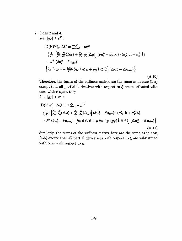
2. Sides 2 and 4: 2-a. IYTI < eT :

D(VW)c l:l.U = 2:~1 -wtk

{ fr [~ J!,(l:l.x) + ~ J!,(l:l.y)] {t5u~- t5noos) ·{at D.+ a~ t) -Jk {t5u~- t5uoos)·

[kN D.® D.+~ ([}Tt ®D.+ 9Ni ® t)] {l:l.u~ -l:l.uoos)}

{A.lO) Therefore, the terms of the stiffness matrix are the same as in case {1-a) except that all partial derivatives with respect to e are substituted with ones with respect to 11·

2-b. IYTI > eT :

D(VW)c l:l.U = I:f=I -wtk

{ fr [~ !, (l:l.x) + ~ J!,(l:l.y)] {t5u~- blloos) · (at D.+ a~ t)

-Jk (t5u~- t5uobs) · [ kN D.® D.+ JL kN sign(gT) t ®D.)] (l:l.u~ -l:l.Uoos)}

(A.ll) Similarly, the terms of the stiffness matrix here are the same as in case (1-b) except that all partial derivatives with respect toe are substituted with ones with respect to 11·

129

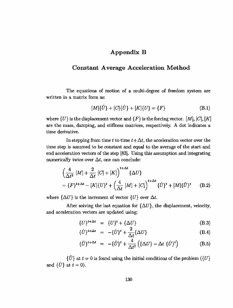
Appendix B

Constant Average Acceleration Method

The equations of motion of a multi-degree of freedom system are written in a matrix form as:

[M]{U} + [C]{U} + [K]{U} = {F} (B.l)

where {U} is the displacement vector and {F} is the forcing vector. [M], [C], [K] are the mass, damping, and stiffness matrices, respectively. A dot indicates a time derivative.

In stepping from timet to time t+ll.t, the acceleration vector over the time step is assumed to be constant and equal to the average of the start and end acceleration vectors of the step [83]. Using this assumption and integrating numerically twice over ll.t, one can conclude:

( 4 2 )t+at

fl.t2 [M] + fl.t [C] + [K] { fl.U}

( 4 )t+at

{F}t+at- [K]{U}t + ll.t [M] + [C] {U}t + [M]{U}t (B.2)

where {fl.U} is the increment of vector {U} over ll.t.

After solving the last equation for {fl.U}, the displacement, velocity, and acceleration vectors are updated using:

{U}t+at - {U}t + { fl.U} (B.3)

{U}t+at - -{U}t + ~t {fl.U} (B.4)

{U}t+at -{U}t + fl.~2 ( {fl.U}- ll.t {U}t) (B.5)

{U} at t = 0 is found using the initial conditions of the problem ( {U} and {U} at t = 0).

130

BIBLIOGRAPHY

[I] J. E. Long. Bearings in Structural Engineering. Newnes-Butterworths, London, 197 4.

[2] A. N. Gent and P. B. Lindley. "The Compression of Bonded Rub­ber Blocks". Proceedings of the Institution of Mechanical Engineers, 173(3):111-117, 1959.

[3] A. N. Gent and E. A. Meinecke. "Compression, Bending, and Shear of Bonded Rubber Blocks". Polymer Engineering and Science, 10(1):48-53, January 1970.

[4] J. F. Stanton and C. W. Roeder. Elastomeric Bearings Design, Construc­tion, and Materials. Technical Report NCHRP #248, 'Iransportation Re­search Board, Washington, D.C., August 1982.

[5] C. W. Roeder, J. F. Stanton, and A. W. Taylor. Performance of Elas­tomeric Bearings. Technical Report NCHRP #298, 'fransportation Re­search Board, Washington, D.C., October 1987.

[6] P. Lindley. "Natural Rubber Structural Bearings". In Joint Sealing and Bearing Systems for Concrete Structures, SP-70, pages 353-378, ACI, De­troit, 1981.

[7] P. K. Freakley and A. R. Payne. Theory and Practice of Engineering with Rubber. Applied Science Publishers Ltd., London, 1978.

[8] E. V. Clark and K. Moultrop. "Load-Deformation Characteristics of Elas­tomeric Bridge Bearing Pads". Highway Research Record, 34:9Q-116, 1963.

[9] C. J. Derham and A. G. Thomas. "The Design and Use of Rubber Bear­ings for Vibration Isolation and Seismic Protection of Structures". Eng. Struct., 2:171-175, July 1980.

131

[10] M. S. Chalhoub and J. M. Kelly. "Sliders and Tension Controlled Rein­forced Elastomeric Bearings Combined for Earthquake Isolation". Earth­quake Engineering and Structural Dynamics, 19(3):333-344, April 1990.

[11] R. L. Wilkison. Design of Neoprene Bearing Pads. Technical report, E. I. duPont de Nemours & Co., Delaware, U.S.A., April1959.

[12] J. F. Stanton and C. W. Roeder. "Elastomeric Bearings: An Overview". Concrete International, 14(1):41-46, January 1992.

[13] I. Schrage. "Anchoring of Bearings by Friction". In Joint Sealing and Bearing Systems for Concrete Structures, SP-70, pages 197-213, ACI, De­troit, 1981.

[14] A. W. Taylor, A. N. Lin, and J. W. Martin. "Performance of Elastomers in Isolation Bearings: A Literature Review". Earthquake Spectra, 8(2):279-303, 1992.

[15] S. L. Rosen. Fundamental Principles of Polymeric Materials for Practicing Engineers. Barnes & Noble, New York, 1971.

[16] G. R. Hamed. "Materials and Components". In A. N. Gent, editor, En­gineering with Rubber, pages 13-31. Hanser Publishers, 1992.

[17] A. N. Gent, R. L. Henry, and M. L. Roxbury. "Interfacial Stresses for Bonded Rubber Blocks in Compression and Shear". Journal of Applied Mechanics, Transactions of the ASME, 41(4):855-859, December 1974.

[18] F. Conversy. "Appareils d' Appui en Caoutchouc Frette". Annales des Ponts et Chaussies, 6, November-December 1967.

[19] P. B. Lindley. "Load-Compression Relationships of Rubber Units". Jour­nal of Strain Analysis, 1(3):19Q-195, 1966.

[20] B. P. Holownia. "Stiffness of Rubber Blocks in Contact with Different Surfaces". Plastics and Rubber Processing and Applications, 3(1):9-12, 1983.

[21] B. P. Holownia. "Effect of Poisson's Ratio on Bonded Rubber Blocks". Journal of Strain Analysis, 7(3):236-242, 1972.

132

[22] C. W. Roeder and J. F. Stanton. "State-of-the-Art Ela.stomeric Bridge Bearing Design". ACI Structural Journal, 88(1):31-41, January-February 1991.

[23] Transportation Research Board. Bridge Bearings. Technical Report NCHRP #41, Transportation Research Board, Wa.shington, D.C., 1977.

[24] J. C. Minor and R. A. Egen. Elastomeric Bearing Research. Technical Report NCHRP #109, Highway Research Board, Wa.shington, D.C., 1970.

[25] C. W. Roeder, J. F. Stanton, and T. Feller. Low Temperature Behavior and Acceptance Criteria for Elastomeric Bridge Bearings. Technical Re­

port NCHRP #325, Transportation Research Board, Washington, D.C., December 1989.

[26] M. L. Soni. A Microstructure Continuum Theory for Laminated Elastic Composites. PhD thesis, The University of Texa.s at Austin, Austin, TX 78712, May 1977.

[27] L. R. Herrmann, R. Hamidi, F. Shafigh-Nobari, and C. K. Lim. "Nonlinear Behavior of Elastomeric Bearings: I. Theory". Journal of Engineering Mechanics, ASCE, 114(11):1811-1830, November 1988.

[28] L. R. Herrmann, R. Hamidi, F. Shafigh-Nobari, and A. Ramaswamy. "Nonlinear Behavior of Elastomeric Bearings: II. FE Analysis and Ver­ification". Journal of Engineering Mechanics, ASCE, 114(11):1831-1853, November 1988.

[29] L. R. Herrmann. "Elasticity Equations for Incompressible and Nearly Incompressible Materials". AIAA J., 3(10):1896-1900, 1965.

[30] R. Glowinski and P. Le Tallec. "Finite Elements in Nonlinear Incompress­ible Elasticity''. In J. T. Oden and G. F. Carey, editors, Finite Elements, Volume V: Special Problems in Solid Mechanics, pages 67-93. Prentice­Hall, Englewood Cliffs, N.J., 1984.

[31] T. Endo, J. T. Oden, E. B. Becker, and T. Miller. "A Numerical Analysis of Contact and Limit-point Behavior in a Class of Problems of Finite Elastic Deformations". Computers & Structures, 18(5):899-910, 1984.

133

[32] J. Fine, E. B. Becker, , and T. Miller. Finite Element Analysis and the Design of Rubber Components. Short course, Mechanics Software Inc., Austin, Texas, January 19-21, 1993.

[33] J. C. Simo and R. L. Taylor. "Quasi-Incompressible Finite Element Elas­ticity in Principal Stretches. Continuum Basis and Numerical Algorithms". Computer Methods in Applied Mechanics and Engineering, 85:273-310, 1991. North-Holland.

[34] A. S. Aly. A Finite Element Analysis for Problems of Large Strain and Large Displacement. PhD thesis, The University of Texas at Austin, Austin, TX 78712, May 1981.

[35] T. Miller. A Finite Element Study of Instabilities in Rubber Elasticity. PhD thesis, The University of Texas at Austin, Austin, TX 78712, De­cember 1982.

[36] T. J. R. Hughes. The Finite Element Method. Prentice-Hall, Englewood Cliffs, New Jersey, 1987.

[37] 0. C. Zienkiewicz and R. L. Taylor. The Finite Element Method, volume 1. McGraw-Hill Book Company, London, fourth edition, 1991.

[38] K. J. Bathe. Finite Element Procedures in Engineering Analysis. Prentice­Hall, Englewood Cliffs, New Jersey, 1982.

[39] B. A. Szabo. "The p- and h-p Versions of the Finite Element Method in Solid Mechanics". Computer Methods in Applied Mechanics and Engi­neering, 80:185-195, 1990. North-Holland.

[40] I. Babuska and M. Suri. "The p- and h-p Versions of the Finite Element Method, An Overview". Computer Methods in Applied Mechanics and Engineering, 80:5-26, 1990. North-Holland.

[41] 0. N. Hamzeh. The Fast Adaptive Composite Grid Method in Finite Element Applications. Master's thesis, Colorado State University, Fort Collins, CO 80523, Fall 1990.

134

[42] I. Babuska, B. A. SzabO, and I. N. Katz. "The p-version of the Finite Element Method". SIAM Journal for Numerical Analysis, 18:512-545, June 1981.

[43] I. Babuska and M. R. Dorr. "Error Estimates for the Combined h and p­version of the Finite Element Method". Numerical Mathematics, 37:257-277, 1981.

[44] B. SzabO and I. Babuska. Finite Element Analysis. John Wiley & Sons, 1991.

[45] 0. C. Zienkiewicz and R. L. Taylor. The Finite Element Method, volume 2. McGraw-Hill Book Company, London, fourth edition, 1991.

[46] I. Babu8ka, M. Griebel, and J. Pitkaranta. "The Problem of Selecting the Shape Functions for a p-type Finite Element". International Journal for Numerical Methods in Engineering, 28:1891-1908, 1989.

[47] I. Babuska, B. A. SzabO, and R. L. Actis. "Hierarchic Models for Lami­nated Composites". International Journal for Numerical Methods in En­gineering, 33:503-535, 1992.

[48] B. A. Szabo. "Stress Computations for Nearly Incompressible Materials". In J. K. Nelson, Jr., editor, Computer Utilization in Structural Engineer­ing. Proceedings of the Sessions at the Structures Congress 89, pages 306-313, ASCE, New York, N.Y., May 1989.

[49] B. A. Szabo, L BabuSka, and B. K. Chayapathy. "Stress Computations for Nearly Incompressible Materials by the p-version of the Finite Element Method". International Journal for Numerical Methods in Engineering, 28:2175-2190, 1989.

[50] K. Kato, N. S. Lee, and K. J. Bathe. "Adaptive Finite Element Analysis of Large Strain Elastic Response". Computers & Structures, 4 7( 4/5):829-855, 1993.

135

[51] D. A. Dunavant. "Experience with the p-version Program PROBE". In Computer Utilization in Structural Engineering. Proceedings of the Ses­sions at the Structures Congress 89, pages 314-321, New York, N.Y., 1989. ASCE.

[52] T. Y. Chang, A. F. Saleeb, , and S. C. Shyu. "Finite Element Solutions of Two-dimensional Contact Problems Based on a Consistent Mixed For­mulation". Computers & Structures, 27(4):455-466, 1987.

[53] S. Timoshenko and J. N. Goodier. Theory of Elasticity. McGraw-Hill, New York, 1951.

[54] J. Hallquist and D. Nike. An Implicit, Finite Deformation, Finite-element Code for Analyzing the Static and Dynamic Response of Two-dimensional Solids. Technical Report UCRL-52678, University of California-Lawrence Livermore National Laboratory, 1979.

[55] P. Wriggers, T. Vu Van, , and E. Stein. "Finite Element Formulation of Large Deformation Impact-Contact Problems with Friction". Computers & Structures, 37(3):319-331, 1990.

[56] J. W. Ju and R. L. Taylor. "A Perturbed Lagrangian Formulation for the Finite Element Solution of Nonlinear Frictional Contact Problems". Journal of Theoretical and Applied Mechanics, 7(1):1-14, 1988.

[57] K. J. Bathe and S. Mijailovich. "Finite Element Analysis of Frictional Con­tact Problems". Journal of Theoretical and Applied Mechanics, 7(1):31-45, 1988. Special issue.

[58] M. G. Katona. "A Simple Contact-Friction Interface Element with Ap­plication to Buried Culverts". International Journal for Numerical and Analytical Methods in Geomechanics, 7:371-384, 1983.

[59] K. J. Bathe and A. Chaudhary. "A Solution Method for Planar and Axisymmetric Contact Problems". International Journal for Numerical Methods in Engineering, 21:65-88, 1985.

136

[60] B. Nour-Omid and P. Wriggers. "A Two-Level Iteration Method for Solu­tion of Contact Problems". Computer Methods in Applied Mechanics and Engineering, 54:131-144, 1986. North-Holland.

[61] M. J. Saran and R. H. Wagoner. "A Consistent Implicit Formulation for Nonlinear Finite Element Modeling with Contact and Friction: Part I-Theory". Journal of Applied Mechanics, ASME, 58:499-506, June 1991.

[62] J. A. C. Martins, J. T. Oden, and F. M. F. SimOes. "A Study of Static and Kinetic Friction". International Journal of Engineering Science, 28(1):29-92, 1990.

[63] A. Ibrahimbegovic and E. L. Wilson. "Unified Computational Model for Static and Dynamic Frictional Contact Analysis". International Journal for Numerical Methods in Engineering, 34:233-247, 1992.

[64] R. W. Ogden. Non-Linear Elastic Deformations. Ellis Horwood Series in Mathematics and its Applications. Ellis Horwood, England, 1984.

[65] M. E. Gurtin. An Introduction to Continuum Mechanics. Mathematics in Science and Engineering Series. Academic Press, New York, NY, 1981.

[66] L. R. G. Theloar. The Physics of Rubber Elasticity. Oxford University Press, London, third edition, 1975.

[67] 0. H. Yeoh. "Some Forms of the Strain Energy Function for Rubber". Rubber Chemistry and Technology, 66(5):754-771, Nov.-Dec. 1993.

[68] TEXPAC-NL, A Finite Element Code for Elastomeric Analysis. TEXas Polymer Analysis Corp., Dallas, Texas, 1987. developed by: Mechanics Software Inc.

[69] R. S. Rivlin. "Large Elastic Deformations". In F. R. Eirich, editor, Rhe­ology: Theory and Applications, Vol.l. Academic Press, New York, 1956.

[70] Y. J. Arditzoglou. Test Methods for Elastomeric Bearings on Bridges. Master's thesis, The University of Texas at Austin, Austin, TX 78712, May 1994.

137

[71] J. V. Muscarella. Analysis and Design of Elastomeric Bearings. PhD thesis, The University of Texas at Austin, Austin, TX 78712, May 1995.

[72] F. P. Bowden and D. Tabor. Friction, An Introduction to Tribology. An­chor Science Study Series. Anchor Press/Doubleday, Garden City, New York, 1973.

[73] D. F. Moore. The Friction and Lubrication of Elastomers. International Series of Monographs on Materials Science and Technology. Pergamon Press, Oxford, England, first edition, 1972.

[7 4] D. F. Moore. Principles and Applications of Tribology. International Series in Materials Science and Technology. Pergamon Press, Oxford, England, first edition, 1975.

[75] H. W. Kummer. Unified Theory of Rubber and Tire Friction. Technical Report ERB B-94, The Pennsylvania State University, University park, Pennsylvania, July 1966.

[76] G. M. Bartenev and V. V. Lavrentev. Friction and Wear of Polymers. Tri­bology Series. Elsevier Scientific Publishing Company, Amsterdam, 1981. Translated by: D. B. Payne.

[77] D. D. Fuller. Theory and Practice of Lubrication for Engineers. John Wiley & Sons, second edition, 1984.

(78] M. B. Peterson and M. Kanakia. "Friction with Solid Lubricant Films". In F. F. Ling and C. H. T. Pan, editors, Approaches to Modeling of Friction and Wear, page 102. Columbia University, N.Y., Springer-Verlag, Decem­ber 17-19 1986.

(79] J. R. Libby. "Four Case Histories: Elastomeric Bearing Pad Connections in Precast Concrete Parking Structures". Concrete International: Design and Construction, 9(9):5Q-58, September 1987.

(80] American Association of State Highway and Transportation Officials. Standard Specifications for Highway Bridges. 15th edition, AASHTO, Washington, D.C., 1992.

138

[81] J. D. Ferry. Viscoelastic Properties of Polymers. John Wiley & Sons, second edition, 1970.

[82] B. A. English. Elastomeric Bearings: Background Information and Field Studies. Master's thesis, The University of Texas at Austin, Austin, TX 78712, May 1993.

[83] M. Paz. Structural Dynamics: Theory and Computation. Van Nostrand Reinhold Co., New York, second edition, 1985.

139