HAL Id: hal-01575669https://hal.archives-ouvertes.fr/hal-01575669

Submitted on 14 Feb 2018

HAL is a multi-disciplinary open accessarchive for the deposit and dissemination of sci-entific research documents, whether they are pub-lished or not. The documents may come fromteaching and research institutions in France orabroad, or from public or private research centers.

L’archive ouverte pluridisciplinaire HAL, estdestinée au dépôt et à la diffusion de documentsscientifiques de niveau recherche, publiés ou non,émanant des établissements d’enseignement et derecherche français ou étrangers, des laboratoirespublics ou privés.

Analysis of digitized 3D mesh curvature histograms forreverse engineering

Silvère Gauthier, William Puech, Roseline Bénière, Gérard Subsol

To cite this version:Silvère Gauthier, William Puech, Roseline Bénière, Gérard Subsol. Analysis of digitized 3D meshcurvature histograms for reverse engineering. Computers in Industry, Elsevier, 2017, 92-93, pp.67-83.10.1016/j.compind.2017.06.008. hal-01575669

Analysis of digitized 3D mesh curvature histograms forreverse engineering

S. Gauthiera,b, W. Puecha, R. Beniereb, G. Subsola

aLIRMM Laboratory, UMR 5506, CNRS, University of Montpellier, 860 rue de St Priest,Montpellier, France

bC4W, 219 rue Le Titien, Montpellier, France

Abstract

Today, it has become more frequent and reasonably easy to digitize the surfaceof 3D objects. However, the obtained results are often inaccurate and noisy.In this paper, we present an efficient method to analyze a curvature histogramfrom a digitized 3D surface using a real object. Moreover, we propose to use thecurvature histogram analysis for many steps of a reverse engineering process,which can be used to retrieve a CAD model from a digitized one for example.Our objective is to design a fast and fully automated method, which is seldomseen in reverse engineering. Experimental results applied on digitized 3D meshesshow the efficiency and the robustness of our proposed method.

Keywords: 3D Mesh, digitized, curvature, distribution, reverse engineering

c©2017. This manuscript version is made available under the CC-BY-NC-ND 4.0 licensehttp://creativecommons.org/licenses/by-nc-nd/4.0/

Formal publication: https://doi.org/10.1016/j.compind.2017.06.008

1. Introduction

The availability of 3D scanners has increased the fast development of appli-cations in Computed-Aided Design (CAD), reverse engineering, medicine andinspection. Many 3D processes use the objects shape, like segmentation, recog-nition or classification for example. In the production line of manufactured5

objects, steps can be distributed to many partners, and during the process,some data can be lost. An industrial reverse engineering application aims toreconstruct an object as a combination of geometric primitives, from a digitized3D mesh or 3D point cloud [1, 2]. For mechanical objects, we search for planes,spheres, cylinders and cones, but also torus and more specifically developable10

or ruled surfaces. This can lead to quality control or object modification issuesfor example. To reconstruct the initial geometry, we must take into accountthe shape of the objects and their relationship with each other. But an objectshape can be very complex, and the measured data can often be noisy. So, weneed robust 3D descriptors to accurately define the objects shape.15

Preprint submitted to Computers in Industry June 26, 2017

In previous work, geometry descriptors like the curvatures [3, 4] allow us todeal with the 3D mesh shape. But the curvature is computed locally, while it isoften necessary to characterize the shape globally. To do this, we can constructcurvature distributions [5, 6] and analyze them.

In this paper, we propose a method based on the analysis of a digitized 3D20

mesh curvature histogram. We use the curvature approximation from Beniereet al. [7] who incorporates two other methods [8, 9]. Then, a distribution is con-structed continuously by a kernel estimation from all of the curvature values.Finally, an accurate curvature distribution analysis is realized. In the distribu-tion, we propose to search for peaks and valleys, and compute some statistics25

depending on the chosen application. Indeed, curvature distribution approxi-mately describes the objects shape, so these distributions can be useful to manyapplications. In this paper, we propose to use a curvature histogram to segment3D meshes, detect primitive type and measure the quality of the mesh.

This paper is organized as follows. Previous work in this topic is presented30

in Section 2. In Section 3, we present in detail our distribution construction andanalysis. Section 4 is dedicated to three uses of curvature distribution, whichare mesh segmentation, primitive type detection with tolerances adaptationand mesh quality evaluation. In Section 5, we apply our proposed analysison digitized 3D surfaces of real objects and we show that our analysis hugely35

improves the obtained results. Finally, we conclude and propose directions forfuture research in Section 6.

2. Previous work

We present in Section 2.1 previous work on curvatures and distributions.Then, we show three fields in 3D mesh processing: mesh segmentation in Sec-40

tion 2.1.1, geometric primitive type detection in Section 2.1.2 and mesh qualityevaluation in Section 2.1.3.

2.1. Curvature distribution

Intuitively, curvature quantifies the deviation between a curve and a straightline, or between a surface and a plane in 3D. The curvature of a 2D curve at a45

point P equals the inverse of the osculating circle radius r at P . The osculatingcircle is the circular arc which best approximates the curve around P (Fig. 1.a).

On a 3D surface, an infinity of curvature directions exists around the normalvector of P (Fig. 1.b). So, we need to distinguish particular curvatures. Prin-cipal curvatures are the minimum and maximum curvatures. Mean curvature50

and Gaussian curvature equal respectively the mean and the product of princi-pal curvatures. The Euler formula gives the continuous curvature at a point Pfor each tangent vector ti:

kn(ti) = kmaxcos2(θ) + kminsin

2(θ), (1)

where kmax and kmin are the principal curvatures, and θ is the angle betweenthe maximum principal direction ~dmax and the direction of kn. But since a mesh55

2

Figure 1: Curvature representation on: a) 2D curves and b) 3D surfaces.

is a discrete object, we need to approximate the curvature from a point cloud.Chen and Schmitt [8] compute “discrete” curvatures at P with the Meusniertheorem:

kn(t) = kC ∗ cos(θ), (2)

where kC is the curvature at P of the curve obtained by intersection betweenthe surface and a plane PC , and θ is the angle between the normal at P and60

the normal of the plane PC . Each neighbor pair of P defines a plane with P ,and the curvature circle is the circumscribed circle of the three points. A linearregression is then applied on all discrete curvatures to retrieve approximatedprincipal curvatures.

Dong and Wang [9] compute discrete curvatures with:65

kn(t) =< Pi − P,Ni −N >

||Pi − P ||2, (3)

where Pi is a neighbor of P with a normal Ni, and ~t the projection of ~PiP on thetangent plane of P . A linear regression is also applied on all discrete curvatures,but with a coefficient fixed to the maximum computed value.

Beniere et al. [2] compute discrete curvatures with the formula 3 for eachneighbor of P , and apply the linear regression of [8]. For our proposed ap-70

proach, we prefer to use this approximation because it is more accurate. Indeed,equation 3 uses each neighbor independently and avoids some curve distortion.Moreover, fixing a linear regression coefficient when we do not know if we havecomputed the real maximum curvature is dangerous. Curvatures are often usedto caracterize surface shape [10, 11]. So, for example, it is possible to analyze a75

shape to detect saliency [12] or apply segmentation [13, 5].There are many different types of distributions. But overall, we can dis-

tinguish discrete and continous distributions. A discrete distribution is oftenrepresented by a histogram, as illustrated in Fig. 2.a. On the other hand, con-tinous distributions correspond to mathematical models. Common models are80

Gaussian or Normal distributions (Fig. 2.b).

3

Figure 2: a) Discrete and b) Continuous distribution samples.

In our case, computed curvature values are real. So, it is necessary to approx-imate a discrete distribution with a continuous model. Most of the time, modelsare optimized from the measured data. Model optimization estimates the pa-rameters of a density function by maximizing the joint likelihood of the observed85

samples to be generated by this model. A common optimization algorithm isthe Expectation-Maximisation (EM) [14]. For example, these distributions canbe used in image processing to improve compression [6], for perceptual hashingsystems [15], or even automatic image thresholding [16].

Previous methods in 3D mesh processing proposed to use distributions[17, 5].90

For example, Demarsin et al. [17] compute an absolute mean curvature his-togram used to extract object edges. They analyze many histogram resolutionsto define a sufficient bin number. However, Chen and Feng [5] construct a signedmean curvature histogram, then apply a Laplacian smooth modifier and analyzethe histogram to segment the object. They can separate homogeneous intervals95

by histogram analysis. But the main limitation of these two methods is that thehistogram is constructed with a discrete approach, whereas curvature values arereal. To extend their methods, we can construct a histogram by optimisationor kernel estimation for example.

2.1.1. Segmentation100

A segmentation is a partitioning of a digital image, a 3D mesh or a 3D pointcloud in several regions, as illustrated in Fig. 3. For 3D objects, we distinguishbetween cloud-based [18] and mesh-based approaches [19].

Many different 3D mesh segmentation algorithms have been published [20,21], but each segmentation gives more or less good results depending on the cho-105

sen application. Most of the time, a segmentation brings together points withsimilar criteria. For example, the segmentation can be based on a waterfall [22],hierarchical clustering [23], iterative merging [24] or remeshing [25]. In reverseengineering, the best results are reached when using curvatures, because prim-itives are extracted from curvatures analysis. Some methods use curvatures110

to segment by discontinuities [1, 5], clustering [26], or to better digitize [27],but they are often not robust enough around object edges or are sensitive tonoise [13, 2]. Indeed, curvatures are often inaccurate around object edges be-cause adjacent points can run over many different primitives. Moreover, weare searching for a fully automatic method, so we cannot use parameters like a115

4

Figure 3: Examples of mesh segmentation from [19]: a) A section-type segmentation, b) asurface-type segmentation.

cluster number [28].The edge extraction of Demarsin et al. [17] is interesting, but it is not entirely

automatic. Indeed, they compute an absolute mean curvature histogram anddefine a threshold leading to edge extraction. Then, they ask for user helpto validate the result or compute another threshold. To extend this threshold120

computation, we can normalize the curvature and fix the histogram range.Chen and Feng [5] propose to construct the mean curvature histogram, and

then to apply a Laplacian smooth modifier. After, they compute valleys onthe histogram, which define segmentation thresholds. Finally, they retrieve theisolated regions and improve their boundaries. But their method is limited since125

they do not have a single primitive per submesh. To extend this segmentation,we can apply a recursive extraction of salient edges.

2.1.2. Primitive type detection

Primitive extraction starts from an initial set of measured data and buildsderived values, which are primitives (Fig 4).130

Figure 4: a) Original 3D mesh, b) Curvature: planar (green), spherical (yellow), convex (blue)and concave (red), c) Point areas, d) Extracted primitives [2].

We generally search for planes, spheres and cylinders because they are themost common primitives contained in mechanical objects, but we can also search

5

for cones, torus or ruled surfaces for example. Primitive extraction can be basedon fitting profiles [1], quadratic surfaces [29] or freeform surfaces [30]. But mostof the time, primitive extraction uses curvature analysis, after a mesh segmen-135

tation [2], with a distribution [31], or even with outlier handling [32]. Sincetwo primitives with identical parameters are not distinguished by their curva-ture, these methods cannot directly handle primitive positions. But curvature isrobust to noise, and can be analyzed locally to extract each primitive separately.

The limit of these methods is that they can not estimate the primitive type140

before extraction. To detect this primitive type, we propose to analyze theprincipal curvature distributions.

2.1.3. Noise and mesh quality evaluation

In many 3D processes, it is important to handle noise properly to avoiddistorted representation. But noise characterization depends on the chosen145

scanner. In fact, noise characterization for depth sensors [33] and for laserbeams [34] are different. So, digitization noise estimation is difficult. Most ofthe time, methods presume a Gaussian and isotropic noise, which does not re-flect reality. To properly deduce the real noise type, it is necessary to know theobject shape before the analysis. But in case of digitized meshes, we cannot150

know this shape. Moreover, many different noises can be present at the sametime. In Fig. 5, we apply different values of gaussian noise to a sphere andcompare curvature histograms. We show that curvature distributions of noisyspheres have a gaussian shape, which is related to the noise type.

Figure 5: Spheres of radius r = 10 with gaussian noise and their corresponding mean curvaturehistogram: a) original sphere, b) σ = 0.01, c) σ = 0.1.

We can also introduce an estimation for the roughness of the surface [35],155

which is defined by a local analysis of the curvature values. Like the noise oncoordinates, the roughness can be difficult to characterize since it depends alsoon the object material and the digitization. Sometimes, roughness can quantifylocally the noise.

6

3. Proposed curvature distribution analysis160

Our proposed method first computes a discrete curvature on each vertexof the initial 3D mesh. This method constructs a continuous estimated andnormalized histogram for each curvature (Section 3.1), then analyzes it (Sec-tion 3.2). An overview of our proposed method is illustrated Fig. 6.

Figure 6: Method overview.

We provide, for example, a peak and valley extraction used for segmentation165

(Section 4.1). In the same way, some statistics computed on each histogram areuseful to adapt geometric extraction tolerances (Section 4.2) or measure thequality of the mesh (Section 4.3).

3.1. Probability curvature distribution

A probability distribution assigns a probability to each measurable subset of170

the possible outcomes of a random experiment, survey, or procedure of statisticalinference. We can represent a probability distribution by a histogram. But todefine the probability distributions for the simplest cases, we need to distinguishbetween discrete and continuous random variables. In the discrete case, we caneasily assign a probability to each possible value. By contrast, when a random175

variable like curvature takes values from a continuum, then probabilities can benonzero only if they refer to intervals.

To approximate continuous curvatures on a discrete 3D mesh, we use themethod proposed by Beniere et al. [2]. In our case, meshes can be definedwith different scales and can give different curvature ranges. So, to construct180

7

curvature histograms which can be compared between many objects, we mustnormalize curvature values with each mesh (Section 3.1.1). Moreover, curvaturevalues are real, so it is more suitable to construct a histogram with kernel-estimation for example (Section 3.1.2).

3.1.1. Normalized curvature185

Histograms must have the same range to make a comparison. Indeed, wemust take into account the mesh scale. To homogenize them, curvature valueshave to be normalized. Our method normalizes curvature values by multiplyingthem by the mean edge length of the mesh.

If the object is correctly meshed and edge lengths are equal, we can deduce190

the minimum and maximum possible curvature values, as illustrated in Fig. 7.We propose then to limit the histogram range according to these values.

Figure 7: Minimum and maximum possible for absolute curvature values.

Edge lengths of a digitized mesh are not all equal, but they are similar enoughto not distort the histogram. If a mesh has varying edge lengths, some curvaturevalues can be truncated. Most of the time, there is only a small number of long195

edges, and the histogram is similar with or without these edges.

3.1.2. Kernel estimation

Curvature values are real, so it is more suitable to compute a histogram witha continuous estimation. Our method computes histograms with a kernel-typeestimation. We chose a gaussian kernel because digitized meshes with only one200

primitive often give gaussian-type curvature distributions. This may be relatedto scanner characteristics. We compute the histogram with:

fh(x) =1

n

n∑i=1

Kh(x− xi), (4)

8

where x is the central value of a bin, fh(x) is the quantity inside the bin, n isthe number of points, xi is the ith point and h is the kernel standard deviation.The gaussian kernel is defined by:205

Kh(x− xi) =1

h√

2πe−

12 (

x−xih )2 . (5)

Each bin of the histogram is computed by centering the kernel on it. Then,kernel density estimation (KDE) is applied on each curvature value and addedto the bin. So each bin is computed with a neighborhood defined by the kernelstandard deviation. Fig. 8 shows an example of a normalized mean curvaturedistribution with a kernel deviation h = 0.01.210

Figure 8: Normalized mean curvature kernel-estimated histogram example.

This continuous estimation makes histograms less sensitive to noise and binnumber. Indeed, high frequency fluctuations are naturally smoothed by thekernel. Besides, if the noise deviation is close to or greater than the kerneldeviation, curvature values can be too mixed and histogram analysis is limited.

3.2. Analysis215

Many caracteristics of a histogram can be useful to numerous applications.We can, for example, search for a modal number and positions (named “peaks”here), pattern, sparsity and statistics. In our method, we essentially providerobust peak and valley detection (Section 3.2.1), and use some statistics likemean and standard deviation (Section 3.2.2).220

3.2.1. Peaks and valleys

To detect homogeneous curvature intervals, we need to detect peaks andvalleys in the histogram, as illustrated in Fig. 9.a and Fig. 9.b. A peak definesa dominant curvature value and a pair of two consecutive valleys defines anhomogeneous interval of curvature.225

To detect peaks (or modes), many methods exist like the mean-shift algo-rithm [36]. But these kind of methods can be heavy and do not detect valleys.Therefore, we prefer to use a simple method based on derivatives.

We begin by computing a discrete approximation of the second derivative ofthe histogram:230

D2(i) = H(i+ 1) +H(i− 1)− 2H(i), (6)

with D2(i) the ith second derivative value and H(i) the ith histogram value.

9

Figure 9: Histogram: a) peaks and b) valleys.

Thus, we aim to detect robust peaks and valleys from the second derivative.A peak (resp. a valley) is a bin with a higher (resp. a lower) probability thanthe two adjacent bins. A robust peak (resp. a robust valley) is a bin with thehighest (resp. the lowest) probability in a window. Finally, a robust peak (resp.235

a robust valley) in the second derivative corresponds to a valley (resp. a peak)in the histogram. Our method uses small sliding windows for both peaks andvalleys detection, just to avoid small fluctuations.

3.2.2. Gaussian Mixture Model

We can also estimate our distribution by a Gaussian Mixture Model (GMM),240

which provides mean and standard deviation of each homogeneous interval ofcurvature. To do this, we can use algorithms like K-Means or Bayesian Informa-tion Criterion (BIC) to give a number of gaussian models. Thus, we can use anExpectation-Maximisation algorithm (EM) to optimize these models (Fig. 10.a).

Figure 10: a) Gaussian Mixture Model of a histogram, b) Starting models with peak andvalley detection.

With our peak and valley detection, it is possible to obtain a fast convergence245

of EM. Indeed, we can suppose that the optimal number of models is close toour number of valleys. Moreover, we can compute starting mean and standarddeviation of each model by computing it between each couple of consecutivevalleys (Fig. 10.b). We can see that these models are already close to optimizedones, so fewer iterations are needed to compute them.250

10

4. Curvature distribution applications

Our method can be useful in many applications. This section presents threeapplications which can be used, for example, in a reverse engineering process:digitized 3D mesh segmentation (Section 4.1), primitive type detection withtolerances adaptation (Section 4.2) and mesh quality measurement (Section 4.3).255

4.1. Segmentation

In our case, we work on digitized meshes, with point coordinate inaccuraciesand noise. To correctly segment these, we aim to extract salient object edgesmatching with intersections between geometric primitives (Section 4.1.1). Wecan retrieve isolated and homogeneous regions (Section 4.1.2). Finally, we also260

apply recursivity (Section 4.1.3) to improve results and obtain only one primitivein each submesh. Our proposed segmentation, based on curvature histogramanalysis, is fast and completely automated. Fig. 11 shows an overview of ourproposed segmentation.

Figure 11: Segmentation overview based on the proposed curvature analysis.

4.1.1. Edge extraction265

The edges of an object are the salient mesh areas characterized by a highcurvature. We propose to extract these edges with curvature histogram analy-sis, as described in Section 3. Indeed, high curvatures are on the extremities ofcurvature histograms. To detect and extract the edges, we apply a thresholdingon curvature values. Our method defines two thresholds, matching with the270

extreme left and right valleys of the histogram (Fig. 12). Points with curva-ture between the two thresholds are labelled “uniform”, and others are labelled“edge”.

11

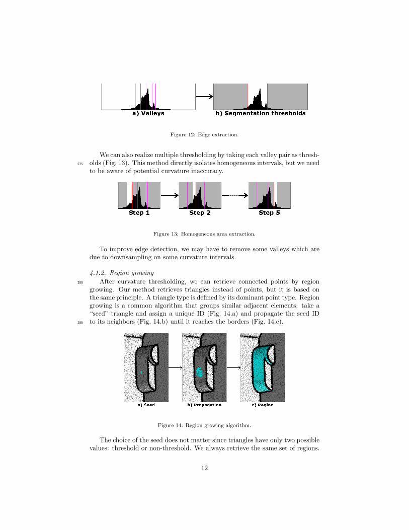
Figure 12: Edge extraction.

We can also realize multiple thresholding by taking each valley pair as thresh-olds (Fig. 13). This method directly isolates homogeneous intervals, but we need275

to be aware of potential curvature inaccuracy.

Figure 13: Homogeneous area extraction.

To improve edge detection, we may have to remove some valleys which aredue to downsampling on some curvature intervals.

4.1.2. Region growing

After curvature thresholding, we can retrieve connected points by region280

growing. Our method retrieves triangles instead of points, but it is based onthe same principle. A triangle type is defined by its dominant point type. Regiongrowing is a common algorithm that groups similar adjacent elements: take a“seed” triangle and assign a unique ID (Fig. 14.a) and propagate the seed IDto its neighbors (Fig. 14.b) until it reaches the borders (Fig. 14.c).285

Figure 14: Region growing algorithm.

The choice of the seed does not matter since triangles have only two possiblevalues: threshold or non-threshold. We always retrieve the same set of regions.

12

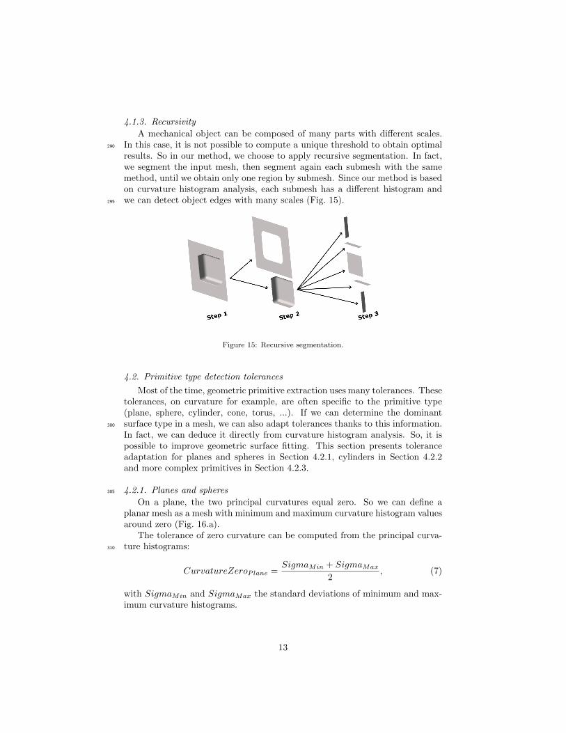
4.1.3. Recursivity

A mechanical object can be composed of many parts with different scales.In this case, it is not possible to compute a unique threshold to obtain optimal290

results. So in our method, we choose to apply recursive segmentation. In fact,we segment the input mesh, then segment again each submesh with the samemethod, until we obtain only one region by submesh. Since our method is basedon curvature histogram analysis, each submesh has a different histogram andwe can detect object edges with many scales (Fig. 15).295

Figure 15: Recursive segmentation.

4.2. Primitive type detection tolerances

Most of the time, geometric primitive extraction uses many tolerances. Thesetolerances, on curvature for example, are often specific to the primitive type(plane, sphere, cylinder, cone, torus, ...). If we can determine the dominantsurface type in a mesh, we can also adapt tolerances thanks to this information.300

In fact, we can deduce it directly from curvature histogram analysis. So, it ispossible to improve geometric surface fitting. This section presents toleranceadaptation for planes and spheres in Section 4.2.1, cylinders in Section 4.2.2and more complex primitives in Section 4.2.3.

4.2.1. Planes and spheres305

On a plane, the two principal curvatures equal zero. So we can define aplanar mesh as a mesh with minimum and maximum curvature histogram valuesaround zero (Fig. 16.a).

The tolerance of zero curvature can be computed from the principal curva-ture histograms:310

CurvatureZeroPlane =SigmaMin + SigmaMax

2, (7)

with SigmaMin and SigmaMax the standard deviations of minimum and max-imum curvature histograms.

13

Figure 16: Principal curvature histograms: a) for a plane and b) for a sphere.

On a sphere, the two principal curvature histogram values are equals andfar from zero. So we can define a spherical mesh as a mesh with minimum andmaximum curvature histogram values which are similar and far from zero, as315

illustrated in Fig. 16.b.The curvature similarity tolerance can be computed with:

LowerBound = min(MuMin − SigmaMin;MuMax − SigmaMax),

UpperBound = max(MuMin + SigmaMin;MuMax + SigmaMax),

SimilarCurvaturesSphere = [LowerBound, UpperBound],

(8)

with (MuMin, SigmaMin) and (MuMax, SigmaMax) the mean and standarddeviation of minimum and maximum curvature histograms respectively.

4.2.2. Cylinders320

On a cylinder, one of the principal curvatures equals zero and the other isfar from zero. So we can define a cylindrical mesh as a mesh with a principalcurvature histogram around zero and the other far from zero (Fig. 17).

Figure 17: Principal curvature histograms for a cylinder.

We can compute a zero curvature tolerance from the histogram with curva-ture values around zero:325

CurvatureZeroCylinder = SigmaZero, (9)

with SigmaZero the standard deviation of the histogram which is around zero.

14

4.2.3. Other primitives

We can also find other primitive signatures in curvature histograms.On a cone, one of the principal curvatures equals zero and the other is

variable (Fig. 18.a). So we can only analyze the zero curvature histogram.330

On a developable surface, one of the curvature equals zero, and the otheris variable. The difficulty is that we may have an inversion of minimum andmaximum curvatures values (Fig. 18.b). A possible solution can be to use theprincipal directions to test the consistency of the two sets of curvatures.

Figure 18: Principal curvature histograms: a) for a cone and b) for a developable surface. Wecan see in hatched orange a constant curvature which can be analyzed.

We can extend this to other surfaces. For example, on a torus or a uniform335

generalized cylinder, one of the curvatures is constant, even if we can have thesame curvature inversion as a developable surface. In all cases, if we can finda constant curvature, we can use it to adapt tolerances and also measure meshquality, as described in Section 4.3.

4.3. Quality measurement340

In many 3D processes, noise leads to distortion and has an impact on resultaccuracy. So to handle this noisy data, we can quantify it on curvature values.

From our curvature distribution approximated by a GMM, as defined inSection 3.2.2, we can retrieve standard deviation of each homogeneous interval,as illustrated in Fig. 19.a, and so estimate a global value representing the noise345

quantity. For example, we can basically use the mean of standard deviations,before or after removing outliers.

In Fig. 19.a, models number 6 and 7 could be outliers because a primitiveleads to a sharp mode, whereas smooth ones are often due to noise. We canalso weight each standard deviation by the number of corresponding points to350

compute the mean.Furthermore, we can also analyse each standard deviation according to the

surface type (primitive), size, position, and so characterize noise more accu-rately. Indeed, the noise depends on the scanner sensor type (depth, laser...),but also on object material, texture, or even scene luminosity and object radi-355

ance. In fact, we can approximate curvature distortion between the digitizedmesh (Fig. 19.a) and the corresponding CAD mesh (Fig. 19.b).

We can also construct many distributions, like minimum, maximum, meanand gaussian curvature histograms, and gather all the informations of thoseto obtain a better characterization. But it is very difficult to have a good,360

15

Figure 19: a) Example of GMM standard deviations. b) Corresponding CAD curvaturedistribution.

accurate and mostly exhaustive method allowing proper noise characterization.In previous work they try to quantify impact of noise on point coordinates, fordepth sensor [33] or laser beam [34] scanners, and propose adapted algorithms.

In our case, we can even characterize the noise on each submesh from a seg-mentation (Section 4.1), and avoid object edge curvature errors in our analysis.365

So, it is possible to measure the noise depending on the mesh area, comparevalues and compute some statistics. This possibly leads to other applicationslike scanner noise characterization [37], for example.

5. Experimental results

Section 5.1 presents three meshes from different scanners. Then, we show370

our results on these meshes, for segmentation in Section 5.2, primitive typedetection in Section 5.3 and quality measurement in Section 5.4.

5.1. Presentation of the three used meshes

For experimental results, we used three digitized meshes from two differentstructured light scanners. The first two come from a first scanner and are375

illustrated in Fig. 20 and Fig. 21 respectively. The third comes from a secondscanner and is illustrated in Fig. 22.

Figure 20: Initial mesh from Scanner 1: Aerospace.

16

Figure 21: Initial mesh from Scanner 1: Moldy.

Figure 22: Initial mesh from Scanner 2: Outlet.

To have an accuracy with an order of magnitude of −3 and center valuesaround zero in the same bin, our method constructs histograms with 1001 bins.These histograms are constructed using a kernel with a standard deviation h =380

0.01. Moreover, we limit our histogram range in the interval [−2; 2] since wenormalize curvature by edge length.

5.2. Segmentation

This section presents results of our segmentation using curvature histogramanalysis. Each figure shows edge extraction and the final submesh set. In385

reverse engineering, our results are very good, since most of the primitives arecorrectly isolated. Indeed, edge extraction is accurate since curvature thresholdsare computed from distribution, and so are adaptative.

The sharp edges of Aerospace are properly detected (Fig. 23.a) and theprimitives are correctly isolated, except for a few tangent ones. We obtain 70390

submeshes and 94.3% of them contain a single primitive (Fig. 23.b).The sharp edges of Moldy are properly detected (Fig. 24.a) and the primitives

are also correctly isolated. We note that freeforms are not over-segmented. Weobtain 48 submeshes and all of them contain a single primitive (Fig. 24.b).

The sharp edges of Outlet are properly detected (Fig. 25.a), except for the395

serrated cylinders, and the primitives are almost all correctly isolated. Weobtain 72 submeshes and all of them contain a single primitive (Fig. 25.b).

As illustrated in Fig. 26, curvatures and thresholds are computed from eachsubmesh at each recursion step. Then, we can continue to segment a submesh

17

Figure 23: a) Edge extraction and b) Segmentation of Aerospace.

Figure 24: a) Edge extraction and b) Segmentation of Moldy.

Figure 25: a) Edge extraction and b) Segmentation of Outlet.

18

until we obtain only one region. We can observe that sharp edges are removed400

from the sharpest to the smoothest. Indeed, each recursion step refines thecurvature thresholds to extract smoother edges.

This recursion has a major impact on the robustness of our method, which isfully automated and adapts to each step. For example, it is possible to correctlysegment an object with heterogeneous noise.405

Figure 26: Example of automatic recursion: a) Edge extraction and b) Segmentation ofManique, c) Edge extraction and d) Segmentation of the first submesh from b), e) Edge ex-traction and f) Segmentation of the first submesh from d). The computed curvature thresholdsare shown in the middle, computed from the corresponding grey part.

We have segmented 30 meshes, with a processor Intel R© CoreTM

i7-4710 CPU@ 2.50GHz. These meshes are extremely varied: they are generated from differ-ent softwares, with or without preprocessing, small or large, more or less noisy.Results are presented in Table 1, where bold names correspond to the threepresented meshes (see section 5.1).410

We can see that our segmentation is fast: less than one minute, except forvery large amounts of triangles. Morover, these times also include curvaturesand mesh topology computation, which represents a large part of the calculation.

To validate our approach, we count the number of submeshes that containonly one primitive. We can see in Table 2 that about 96% of submeshes match415

with only one primitive (remaining 4% can contain similar tangent primitives).Since primitives are correctly isolated, obtained results are suitable for a

reverse engineering application. Indeed, it is more accurate and easy to extract

19

Mesh Triangle T. R.Vase 20 000 <1s 6Fandisk 23 964 <1s 21Lego 24 748 <1s 35Lego small 26 371 <1s 10Cup 55 552 1s 32Yoke 62 276 1s 8Manique 65 090 1s 40Nespresso 71 012 1s 5MediumBolt 89 000 2s 11StripedShoe 100 000 1s 16Connector 195 424 4s 36Outlet 195 853 5s 72Etui 210 963 5s 3Shoe 258 994 3s 4Czslowakei 400 026 8s 162

Mesh Triangle T. R.Part2 414 823 12s 20Chair 500 000 7s 85Gear 500 000 6s 283Aerospace 799 296 16s 70Master 820 793 29s 53Moldy 851 194 13s 48Watertight 921 216 16s 40OilPump 1 064 031 22s 175Carter 1 067 079 34s 108Pump 1 105 570 21s 518Block 1 125 832 33s 113Te 1 297 428 40s 39Splint 2 095 079 1m09s 21Metrologic 2 159 724 1m27s 14ProductPart 3 427 245 2m16s 191

Table 1: Segmentation performances: time (T.) and region number (R.).

Mesh O.P. Total in %Vase 6 6 100Fandisk 20 21 95.2Lego 35 35 100Lego small 10 10 100Cup 32 32 100Yoke 7 8 87.5Manique 33 40 82.5Nespresso 5 5 100MediumBolt 10 11 90.9StripedShoe 16 16 100Connector 33 36 91.7Outlet 72 72 100Etui 3 3 100Shoe 4 4 100Czslowakei 162 162 100

Mesh O.P. Total in %Part2 20 20 100Chair 79 85 92.9Gear 279 283 98.6Aerospace 66 70 94.3Master 49 53 92.5Moldy 48 48 100Watertight 35 40 87.5OilPump 169 175 96.6Carter 106 108 98.1Pump 502 518 96.9Block 111 113 98.2Te 36 39 92.3Splint 19 21 90.5Metrologic 13 14 92.9ProductPart 182 191 95.3

Table 2: Submeshes with only one primitive (O.P.).

20

only one primitive than many on the same mesh, since we do not encountercurvature neighborhood problems or primitive intersections.420

5.3. Primitive type detection

This section presents results of our geometric extraction using curvaturehistogram analysis to detect the primitive type and then adapt the tolerances.Each figure shows extracted primitives with tolerances computed by mesh anal-ysis [7] and curvature analysis. The best mesh analysis results are obtained with425

parameter computations using edge lengths, numbers of points or elements andobject size. We show that our results are better with curvature analysis becausethe tolerances are more accurate and suitable for the purpose. Indeed, we candetermine the main primitive on a mesh (Section 4.2), and particularly on eachsubmesh after segmentation. Since our segmentation gives submeshes with only430

one primitive (Table 2), we can more accurately compute the tolerances for eachprimitive independently.

Aerospace contains 71 primitives with mesh analysis (Fig. 27.a). Some cylin-ders and cones are not extracted because they are often more noisy and so lessstable than planes. We extracted them with curvature analysis and obtained435

105 primitives (Fig. 27.b).

Figure 27: Geometric primitives extraction with a) mesh analysis and b) curvature analysisof Aerospace.

Moldy contains 37 primitives with mesh analysis (Fig. 28.a). The smallcylinders are not extracted because the tolerances must be more accurate thanthose of larger ones. Curvature analysis resolves this problem and leads toextraction of 55 primitives (Fig. 28.b).440

Outlet contains 31 primitives with mesh analysis (Fig. 29.a). All cylindersare missing, because they are too noisy or are serrated on this mesh. Withcurvature analysis, our tolerance adaptation balances the noise and we obtain52 primitives (Fig. 29.b). The serrated cylinders are still not very well rendered,but it is a relatively specific case where the curvature is not constant.445

We have extracted primitives from 30 meshes after segmentation, and com-pared results between the mesh analysis proposed by Beniere et al. [2] and ourproposed curvature analysis in Table 3. These results are related to regionscontaining only one primitive, presented in Table 2.

21

Figure 28: Geometric primitives extraction with a) mesh analysis and b) curvature analysisof Moldy.

Figure 29: Geometric primitives extraction with a) mesh analysis and b) curvature analysisof Outlet.

Mesh F.M.A.[2] F.C.A.

Vase 1 4

Fandisk 14 20

Lego 15 30

Lego small 5 9

Cup 1 4

Yoke 1 3

Manique 28 32

Nespresso 1 4

MediumBolt 4 6

StripedShoe 2 2

Connector 22 28

Outlet 31 52

Etui 2 3

Shoe 2 2

Czslowakei 102 107

Mesh F.M.A.[2] F.C.A.

Part2 11 16

Chair 19 44

Gear 277 279

Aerospace 71 105

Master 0 7

Moldy 37 55

Watertight 8 28

OilPump 17 56

Carter 3 9

Pump 241 263

Block 85 89

Te 20 28

Splint 8 14

Metrologic 0 16

ProductPart 0 62

Table 3: Primitive extraction with Mesh Analysis (F.M.A.) proposed by Beniere et al. [2] andCurvature Analysis (F.C.A.) tolerance adaptation.

22

We can see that curvature analysis leads to a better primitive extraction,450

which is suitable for reverse engineering applications. Indeed, tolerances aremore accurate and adaptative for each submesh, and take the primitive type intoaccount. Moreover, curvature analysis tolerances can balance a larger amountof noise than mesh analysis.

5.4. Quality measurement455

This section presents results of our proposed method using curvature analysisto quantify the noise of a digitized mesh.

Figure 30: Noise in submesh minimum (blue, left), maximum (orange, middle) and mean(grey, right) curvature distributions. Each position on horizontal axis represents a differentsubmesh, and vertical axis shows the corresponding standard deviation values.

We have analyzed the noise of four meshes after segmentation, i.e. the noisein each submesh (Fig. 30). We can see that the noise is often different betweensubmeshes. Moreover, mean curvature is almost always less sensitive to noise.460

These results can lead to a better primitive extraction tolerance adaptation (Sec-tion 4.2), or use in other fields like scanner recognition and authentication [37].

To quantify mesh quality, we can compute statistics on this noise, and thengive a global measurement. For example, we can compute a mean or a pointnumber weighted mean of standard deviations. In the same way, we can compute465

the noise directly from the entire mesh, i.e. without segmentation, from thecurvature distribution GMM (Section 4.3). Since we use a gaussian kernel witha standard deviation h to construct our distribution (Section 3.1.2), we measure

23

a mesh quality by:

σMean < 2h→ Good quality,

2h ≤ σMean < 3h→Middle quality,

σMean ≥ 3h→ Bad quality.

(10)

Mean curvature analysis results on the three used meshes (Section 5.1) are470

compared in Table 4. First of all, we used the entire mesh and a GMM (Sec-tion 3.2.2). Then, we used the segmented mesh with its corresponding sub-meshes (Section 5.2).

a) Without segmentation:Mesh GMM Models Deviation Mean Weighted meanAerospace 3 0.015 0.014 0.015

0.0150.013

Moldy 2 0.023 0.019 0.0220.015

Outlet 3 0.027 0.030 0.0280.0280.034

b) With segmentation:Mesh Submeshes Deviation Mean Weighted meanAerospace 70 min = 0.003 0.013 0.009

max = 0.122Moldy 48 min = 0.001 0.008 0.006

max = 0.086Outlet 72 min = 0.001 0.013 0.010

max = 0.065

Table 4: Measuring the quality: a) without segmentation and b) with segmentation.

Aerospace curvature distribution contains 3 gaussian models which are sim-ilar with a low standard deviation. After segmentation, we obtained a similar475

basic average, but with a better weighted average, suggesting that there arelarge areas that are of a high quality. Globally, this mesh has good qualities.

Moldy curvature distribution contains 2 gaussian models which are differentwith a low to middle standard deviations. After segmentation, the averages aresignificantly better, suggesting that distribution analysis on the entire submesh480

is not adapted. This mesh has an average quality whereas most of its submesheshave a very good quality.

Outlet curvature distribution contains 3 gaussian models which are differentwith two middle and a high standard deviations. After segmentation, the aver-ages are better, suggesting that distribution analysis on the entire mesh is not485

the best approach. This mesh has a high quality when evaluated on submeshes.

24

Globally, we can see through our results that curvature distribution analysison a segmented mesh is better than on the entire mesh. Indeed, the submesheshave homogeneous curvature values and so are consistent for noise evaluation.Although, the entire mesh contains many primitives that are mixed in a unique490

distribution. So, a model can approximate many primitives at the same time.This leads to a degraded approximation and therefore a degraded mesh qualityevaluation.

The noise evaluation, associated with primitive type detection after segmen-tation (Fig. 31), can give a quality coefficient depending on the type.495

Figure 31: Primitive type detection and noise evaluation on Metrologic.

For example, we can compute the quality coefficient with:

if P lane : Qf = SigmaMean,

if Sphere : Qf = SigmaMean,

if Cylinder : Qf = max(SigmaMin, SigmaMax).

(11)

Note that in this object, a submesh contains a torus with two sheres. Ourmethod detects the submesh as spherical, because the minor radius of the torusequals one of the spheres. So, the associated curvature values are similar. How-ever, the major radius leads to a small peak on the maximum curvature his-500

togram, but not significant enough to disturb the method (Fig. 32).In the same way, we can detect submeshes with higher noise than the others

and have a better adaptation of our algorithms. To illustrate this, the upperright plane in Fig. 33 has a slightly higher noise than others for the minimumcurvature distribution.505

We can also use this to improve some processes. For example, we can applya recursion on segmentation with noise handling, depending on the primitive

25

Figure 32: Principal curvature histograms of the submesh containing the torus and the twospheres (Fig.31).

Figure 33: Primitive type detection and noise evaluation on Lego small.

26

type. Indeed, the interpretation of the noise from a plane is slightly differentthan that from a cylinder or a sphere. So, we can construct histograms with adifferent bin number and kernel standard deviation, according to this noise.510

5.5. Case study: quality control

The proposed approaches developed in this paper can be used in many ap-plications. In case of a process using reverse engineering, we can, for example,control the quality of some parts during a manufacturing process, as illustratedFig. 34.515

Figure 34: Example: quality control in a production line.

In fact, we can digitize separately each part of an object, then analyze theircurvature distributions, as presented in Section 3. This allows us to segmentthe digitized meshes (Section 4.1) and then extract the geometric primitives(Section 4.2). Finally, we can measure distances between the primitives andthe initial points (Section 4.3), but also angles and distances between the dif-520

ferent primitives. We can thus quantify the quality of the manufactured object,and eventually stop the manufacturing process if an anomaly is detected, asillustrated Fig. 34.

Since our proposed methods are fast and automatic, this process can be usedin real time for control on a production line.525

6. Conclusion

In this paper, we proposed a new digitized 3D mesh shape analysis basedon curvature analysis. Our proposed method is fast and fully automated, whichis an advantage for industrial applications like reverse engineering for example.Our proposed analysis first constructs a continuous normalized curvature dis-530

tribution, then searches for peak and valley positions and values, and finallyprovides some statistics computed from the curvature distribution.

Our histogram analysis leads to an automatic computation of some parame-ters. So, it can be useful for a large number of processes using many parameters,which often need to be fixed by an expert.535

We chose a reverse engineering process because it is a growing research area,which becomes a hot topic for industrials. Indeed, it is used in many applica-tions since it allows to retrieve directly a parametric model (and thus a CAD

27

model if discretized) from a digitized object. We can also measure object devi-ation for quality control, reconstruct lost models, copy and understand how a540

mechanical object works for example. Moreover, our proposed applications canbe a reliable base for primitive adjustments (like beautification), assembly orsymmetry analysis.

We applied our method on three fields: 3D mesh segmentation, geomet-ric primitive type detection and measurement of quality. We showed that our545

proposed method is accurate and adapted to many fields, through results ondigitized 3D meshes from different scanners.

For 3D mesh segmentation, curvature thresholds are computed from thedistribution to extract the object salient edges. Then, it is possible to retrieveisolated regions corresponding to the object primitives. The final submeshes550

are homogeneous, and each submesh matches with only one primitive. It alsoprovides important information, like the primitive neighborhood through edgeconnectivity. Our segmentation is fast and automatic.

For primitive extraction, the type of the primitive is deduced from the distri-bution and then curvature tolerances are computed to fully adapt them to each555

3D mesh. Then, more primitives are extracted and they are more accurate.For quality measurement, statistics are computed in the first instance on the

entire mesh, and then on each submesh after segmentation. These statistics, likestandard deviation, quantify the noise of a mesh or its submeshes, and so themesh quality. This quality measurement must be interpretated according to the560

distribution construction parameters.We show that our three applications can be associated to improve results.

These three fields show the extensibility and the robustness of our method,which can be used with any distribution to quickly and automatically adapt amethod according to the input data.565

In future work, we will analyze more precisely our curvature distributionconstruction parameters, like bin number or kernel standard derivation, to im-prove computing accuracy. In the same way, we will try to compute multipleprimitive extraction tolerances in the case of 3D meshes with more than one typeof primitive. We can also search for multi-resolution curvature distributions.570

References

[1] Benko, P. and Martin, R. and Varady, T., Algorithms for reverse engi-neering boundary representation models, Computer-Aided Design 33 (11)(2001) 839 – 851. doi:10.1016/S0010-4485(01)00100-2.

[2] Beniere, R. and Subsol, G. and Gesquiere, G. and Le Breton, F. and Puech,575

W., A comprehensive process of reverse engineering from 3D meshes toCAD models, Computer-Aided Design 45 (11) (2013) 1382 – 1393. doi:

10.1016/j.cad.2013.06.004.

[3] Gatzke, T. and Grimm, C., Estimating Curvature on Triangular Meshes,International Journal of Shape Modeling 12 (01) (2006) 1–28. doi:10.580

1142/S0218654306000810.

28

[4] Magid, E. and Soldea, O. and Rivlin, E., A comparison of Gaussian andmean curvature estimation methods on triangular meshes of range imagedata , Computer Vision and Image Understanding 107 (3) (2007) 139 –159. doi:10.1016/j.cviu.2006.09.007.585

[5] Chen, J. and Feng, H., Automatic prismatic feature segmentation ofscanning-derived meshes utilising mean curvature histograms, Virtual andPhysical Prototyping 9 (1) (2014) 45–61. doi:10.1080/17452759.2013.866874.

[6] Masmoudi, A. and Chaoui, S. and Masmoudi, A., A finite mixture590

model of geometric distributions for lossless image compression, Sig-nal, Image and Video Processing 10 (2016) 671–678. doi:10.1007/

s11760-015-0793-1.

[7] Beniere, R. and Subsol, G. and Gesquiere, G. and Le Breton, F. and Puech,W., Recovering Primitives in 3D CAD meshes, SPIE Electronic Imaging595

2011, 3D Imaging, Interaction and Measurement 7864 (2011) 7864 0R–1–9.doi:10.1117/12.872665.

[8] Chen, X. and Schmitt, F., Intrinsic surface properties from surface trian-gulation, Springer Berlin Heidelberg, 1992, pp. 739–743. doi:10.1007/

3-540-55426-2_83.600

[9] Dong, C. and Wang, G., Curvatures estimation on triangular mesh, Journalof Zhejiang University Science 6 (1) (2005) 128–136. doi:10.1631/jzus.2005.AS0128.

[10] Koenderink, J. and van Doorn, A., Surface shape and curvature scales,Image and Vision Computing 10 (8) (1992) 557 – 564. doi:10.1016/605

0262-8856(92)90076-F.

[11] Tang, C. and Medioni, G., Robust Estimation of Curvature Informationfrom Noisy 3D Data for Shape Description in Computer Vision, The Pro-ceedings of the Seventh IEEE International Conference 1 (1999) 426–433.doi:10.1109/ICCV.1999.791252.610

[12] Watanabe, K. and Belyaev, A., Detection of Salient Curvature Featureson Polygonal Surfaces, Computer Graphics Forum 20 (3) (2001) 385–392.doi:10.1111/1467-8659.00531.

[13] Lavoue, G. and Dupont, F. and Baskurt, A., A new CAD mesh segmenta-tion method, based on curvature tensor analysis, Computer-Aided Design615

37 (2004) 975–987. doi:10.1016/j.cad.2004.09.001.

[14] Mclachlan, G. and Krishnan, T., The EM Algorithm and Extensions,Wiley-Interscience, 1996. doi:10.1002/9780470191613.

29

[15] Hadmi, A. and Puech, W. and Ait Es Said, B. and Ai Ouahman, A., Arobust and secure perceptual hashing system based on a quantization step620

analysis, Signal Processing: Image Communication 28 (8) (2013) 929–948.doi:10.1016/j.image.2012.11.009.

[16] Huang, Z. and Chau, K., A new image thresholding method based onGaussian mixture model, Applied Mathematics and Computationdoi:10.1016/j.amc.2008.05.130.625

[17] Demarsin, K. and Vanderstraeten, D. and Roose, D., Meshless Extractionof Closed Feature Lines Using Histogram Thresholding, Computer-AidedDesign and Applications 5 (5) (2008) 589–600. doi:10.3722/cadaps.

2008.589-600.

[18] Sitnik, R. and Blaszczyk, P., Segmentation of unsorted cloud of points data630

from full field optical measurement for metrological validation , Computersin Industry 63 (1) (2012) 30 – 44. doi:10.1016/j.compind.2011.10.

002.

[19] Shamir, A., A survey on Mesh Segmentation Techniques, Computer Graph-ics Forum 27 (6) (2008) 1539–1556. doi:10.1111/j.1467-8659.2007.635

01103.x.

[20] Petitjean, S., A Survey of Methods for Recovering Quadrics in TriangleMeshes, ACM Computing Surveys 2 (34) (2002) 1–61. doi:10.1145/

508352.508354.

[21] Theologou, P. and Pratikakis, I. and Theoharis, T., A Comprehensive640

Overview of Methodologies and Performance Evaluation Frameworks in 3DMesh Segmentation, Comput. Vis. Image Underst. 135 (C) (2015) 49–82.doi:10.1016/j.cviu.2014.12.008.

[22] Delest, S. and Bone, R. and Cardot, H., Fast segmentation of triangularmeshes using waterfall, VIIP ’06 : International Conference on Visualisal-645

ization, Imaging and Image Processing (2006) 308–312.

[23] Garland, M. and Willmott, A. and Heckbert, P., Hierarchical face clusteringon polygonal surfaces, SI3D ’01 : Proceedings of the 2001 Symposium onInteractive 3D Graphics (2001) 49–58doi:10.1145/364338.364345.

[24] Kim, D. and Yun, I. and Lee, S., Boundary-trimmed 3D triangular mesh650

segmentation based on iterative merging strategy, Pattern Recognition5 (39) (2006) 827–838. doi:10.1016/j.patcog.2005.11.022.

[25] Lai, Y. and Zhou, Q. and Hu, S. and Martin, R., Feature sensitive meshsegmentation, SPM ’06 : Proceedings of the 2006 ACM Symposium on Solidand Physical Modeling (2006) 17–25doi:10.1145/1128888.1128891.655

30

[26] Di Angelo, L. and Di Stefano, P., Geometric segmentation of 3D scannedsurfaces, Computer-Aided Design 62 (2015) 44–56. doi:10.1016/j.cad.2014.09.006.

[27] Courtial, A. and Vezzetti, E., New 3D segmentation approach for reverseengineering selective sampling acquisition, The International Journal of660

Advanced Manufacturing Technology 35 (9) (2008) 900–907. doi:10.

1007/s00170-006-0772-3.

[28] Attene, M. and Falcidieno, B. and Spagnuolo, M., Hierarchical meshsegmentation based on fitting primitives, The Visual Computer : Inter-national Journal of Computer Graphics 3 (22) (2006) 181–193. doi:665

10.1007/s00371-006-0375-x.

[29] Wang, J. and Gu, D. and Yu, Z. and Tan, C. and Zhou, L., A Frameworkfor 3D Model Reconstruction in Reverse Engineering, Comput. Ind. Eng.63 (4) (2012) 1189–1200. doi:10.1016/j.cie.2012.07.009.

[30] Weiss, V. and Andor, L. and Renner, G. and Varady, T., Advanced Surface670

Fitting Techniques, Comput. Aided Geom. Des. 19 (1) (2002) 19–42. doi:10.1016/S0167-8396(01)00086-3.

[31] Chen, J. and Feng, H., Idealization of scanning-derived triangle meshmodels of prismatic engineering parts, International Journal on Inter-active Design and Manufacturing (IJIDeM) (2015) 1–17doi:10.1007/675

s12008-015-0262-7.

[32] Tran, T. and Cao, V. and Laurendeau, D., Extraction of Reliable Primitivesfrom Unorganized Point Clouds, 3D Research 6 (4) (2015) 1–12. doi:

10.1007/s13319-015-0076-1.

[33] Pomerleau, F. and Breitenmoser, A. and Liu, M. and Colas, F. and Sieg-680

wart, R., Noise characterization of depth sensors for surface inspections, in:Applied Robotics for the Power Industry (CARPI), 2012 2nd InternationalConference on, 2012, pp. 16–21. doi:10.1109/CARPI.2012.6473358.

[34] Masuda, H. and Tanaka, I. and Enomoto, M., Reliable Surface Extractionfrom Point-Clouds using Scanner-Dependent Parameters, Computer-Aided685

Design and Applications 10 (2) (2013) 265–277. doi:10.3722/cadaps.

2013.265-277.

[35] Lavoue, Guillaume, A Local Roughness Measure for 3D Meshes and ItsApplication to Visual Masking, ACM Trans. Appl. Percept. 5 (4) (2009)21:1–21:23. doi:10.1145/1462048.1462052.690

[36] Carreira-Perpinan, M., A review of mean-shift algorithms for clustering,CoRR abs/1503.00687.

31

[37] Kharboutly, A. and Puech, W. and Subsol, G. and Hoa, D., Improvingsensor noise analysis for CT-Scanner identification, in: Signal ProcessingConference (EUSIPCO), 2015 23rd European, 2015, pp. 2411–2415. doi:695

10.1109/EUVIP.2014.7018385.

32