Deniz Mengu, Yi Luo, Yair Rivenson, and Aydogan Ozcan

Abstract—Optical machine learning offers advantages in

terms of power efficiency, scalability and computation speed.

Recently, an optical machine learning method based on

Diffractive Deep Neural Networks (D2NNs) has been introduced

to execute a function as the input light diffracts through passive

layers, designed by deep learning using a computer. Here we

introduce improvements to D2NNs by changing the training loss

function and reducing the impact of vanishing gradients in the

error back-propagation step. Using five phase-only diffractive

layers, we numerically achieved a classification accuracy of

97.18% and 89.13% for optical recognition of handwritten digits

and fashion products, respectively; using both phase and

amplitude modulation (complex-valued) at each layer, our

inference performance improved to 97.81% and 89.32%,

respectively. Furthermore, we report the integration of D2NNs

with electronic neural networks to create hybrid-classifiers that

significantly reduce the number of input pixels into an electronic

network using an ultra-compact front-end D2NN with a layer-to-

layer distance of a few wavelengths, also reducing the complexity

of the successive electronic network. Using a 5-layer phase-only

D2NN jointly-optimized with a single fully-connected electronic

layer, we achieved a classification accuracy of 98.71% and

90.04% for the recognition of handwritten digits and fashion

products, respectively. Moreover, the input to the electronic

network was compressed by >7.8 times down to 10×10 pixels.

Beyond creating low-power and high-frame rate machine

learning platforms, D2NN-based hybrid neural networks will find

applications in smart optical imager and sensor design.

Index Terms—All-optical neural networks, Deep learning,

Hybrid neural networks, Optical computing, Optical networks,

Opto-electronic neural networks

I. INTRODUCTION PTICS in machine learning has been widely explored due

to its unique advantages, encompassing power efficiency,

speed and scalability[1]–[3]. Some of the earlier work include

optical implementations of various neural network

architectures[4]–[10], with a recent resurgence[11]–[22],

following the availability of powerful new tools for applying

deep neural networks[23], [24], which have redefined the

state-of-the-art for a variety of machine learning tasks. In this

line of work, we have recently introduced an optical machine

D. Mengu, Y. Luo, Y. Rivenson and A. Ozcan are with the Electrical and

Computer Engineering Department, Bioengineering Department, University of California, Los Angeles, CA 90095 USA, and also with the California

NanoSystems Institute, University of California, Los Angeles, CA 90095

USA (email: denizmengu@ucla.edu; yluo2016@ucla.edu; rivensonyair@ucla.edu ; ozcan@ucla.edu)

learning framework, termed as Diffractive Deep Neural

Network (D2NN)[15], where deep learning and error back-

propagation methods are used to design, using a computer,

diffractive layers that collectively perform a desired task that

the network is trained for. In this training phase of a D2NN,

the transmission and/or reflection coefficients of the individual

pixels (i.e., neurons) of each layer are optimized such that as

the light diffracts from the input plane toward the output

plane, it computes the task at hand. Once this training phase in

a computer is complete, these passive layers can be physically

fabricated and stacked together to form an all-optical network

that executes the trained function without the use of any

power, except for the illumination light and the output

detectors.

In our previous work, we experimentally demonstrated the

success of D2NN framework at THz part of the

electromagnetic spectrum and used a standard 3D-printer to

fabricate and assemble together the designed D2NN

layers[15]. In addition to demonstrating optical classifiers, we

also demonstrated that the same D2NN framework can be used

to design an imaging system by 3D-engineering of optical

components using deep learning[15]. In these earlier results,

we used coherent illumination and encoded the input

information in phase or amplitude channels of different D2NN

systems. Another important feature of D2NNs is that the axial

spacing between the diffractive layers is very small, e.g., less

than 50 wavelengths ()[15], which makes the entire design

highly compact and flat.

Our experimental demonstration of D2NNs was based on

linear materials, without including the equivalent of a

nonlinear activation function within the optical network;

however, as detailed in [15], optical nonlinearities can also be

incorporated into a D2NN using non-linear materials including

e.g., crystals, polymers or semiconductors, to potentially

improve its inference performance using nonlinear optical

effects within diffractive layers. For such a nonlinear D2NN

design, resonant nonlinear structures (based on e.g.,

plasmonics or metamaterials) tuned to the illumination

wavelength could be important to lower the required intensity

levels. Even using linear optical materials to create a D2NN,

the optical network designed by deep learning shows “depth”

advantage, i.e., a single diffractive layer does not possess the

same degrees-of-freedom to achieve the same level of

classification accuracy, power efficiency and signal contrast at

the output plane that multiple diffractive layers can

collectively achieve for a given task. It is true that, for a linear

diffractive optical network, the entire wave propagation and

Analysis of Diffractive Optical Neural

Networks and Their Integration with Electronic

Neural Networks

O

diffraction phenomena that happen between the input and

output planes can be squeezed into a single matrix operation;

however, this arbitrary mathematical operation defined by

multiple learnable diffractive layers cannot be performed in

general by a single diffractive layer placed between the same

input and output planes. That is why, multiple diffractive

layers forming a D2NN show the depth advantage, and

statistically perform better compared to a single diffractive

layer trained for the same classification task, and achieve

improved accuracy as also discussed in the supplementary

materials of [15].

Here, we present a detailed analysis of D2NN framework,

covering different parameters of its design space, also

investigating the advantages of using multiple diffractive

layers, and provide significant improvements to its inference

performance by changing the loss function involved in the

training phase, and reducing the effect of vanishing gradients

in the error back-propagation step through its layers. To

provide examples of its improved inference performance,

using a 5-layer D2NN design (Fig. 1), we optimized two

different classifiers to recognize (1) hand-written digits, 0

through 9, using the MNIST (Mixed National Institute of

Standards and Technology) image dataset[25], and (2) various

fashion products, including t-shirts, trousers, pullovers,

dresses, coats, sandals, shirts, sneakers, bags, and ankle boots

(using the Fashion MNIST image dataset[26]). These 5-layer

phase-only all-optical diffractive networks achieved a

numerical blind testing accuracy of 97.18% and 89.13% for

hand-written digit classification and fashion product

classification, respectively. Using the same D2NN design, this

time with both the phase and the amplitude of each neuron’s

transmission as learnable parameters (which we refer to as

complex-valued D2NN design), we improved the inference

performance to 97.81% and 89.32% for hand-written digit

classification and fashion product classification, respectively.

We also provide comparative analysis of D2NN performance

as a function of our design parameters, covering the impact of

the number of layers, layer-to-layer connectivity and loss

function used in the training phase on the overall classification

accuracy, output signal contrast and power efficiency of D2NN

framework.

Furthermore, we report the integration of D2NNs with

electronic neural networks to create hybrid machine learning

and computer vision systems. Such a hybrid system utilizes a

D2NN at its front-end, before the electronic neural network,

and if it is jointly optimized (i.e., optical and electronic as a

monolithic system design), it presents several important

advantages. This D2NN-based hybrid approach can all-

optically compress the needed information by the electronic

network using a D2NN at its front-end, which can then

significantly reduce the number of pixels (detectors) that

needs to be digitized for an electronic neural network to act

on. This would further improve the frame-rate of the entire

system, also reducing the complexity of the electronic network

and its power consumption. This D2NN-based hybrid design

concept can potentially create ubiquitous and low-power

machine learning systems that can be realized using relatively

simple and compact imagers, with e.g., a few tens to hundreds

of pixels at the opto-electronic sensor plane, preceded by an

ultra-compact all-optical diffractive network with a layer-to-

layer distance of a few wavelengths, which presents important

advantages compared to some other hybrid network

configurations involving e.g., a 4-f configuration[16] to

perform a convolution operation before an electronic neural

network.

To better highlight these unique opportunities enabled by

D2NN-based hybrid network design, we conducted an analysis

to reveal that a 5-layer phase-only (or complex-valued) D2NN

that is jointly-optimized with a single fully-connected layer,

following the optical diffractive layers, achieves a blind

classification accuracy of 98.71% (or 98.29%) and 90.04% (or

89.96%) for the recognition of hand-written digits and fashion

products, respectively. In these results, the input image to the

electronic network (created by diffraction through the jointly-

optimized front-end D2NN) was also compressed by more

than 7.8 times, down to 10×10 pixels, which confirms that a

D2NN-based hybrid system can perform competitive

classification performance even using a relatively simple and

one-layer electronic network that uses significantly reduced

number of input pixels.

In addition to potentially enabling ubiquitous, low-power

and high-frame rate machine learning and computer vision

platforms, these hybrid neural networks which utilize D2NN-

based all-optical processing at its front-end will find other

applications in the design of compact and ultra-thin optical

imaging and sensing systems by merging fabricated D2NNs

with opto-electronic sensor arrays. This will create intelligent

systems benefiting from various CMOS/CCD imager chips

and focal plane arrays at different parts of the electromagnetic

spectrum, merging the benefits of all-optical computation with

simple and low-power electronic neural networks that can

work with lower dimensional data, all-optically generated at

the output of a jointly-optimized D2NN design.

II. RESULTS AND DISCUSSION

A. Mitigating vanishing gradients in optical neural network

training

In D2NN framework, each neuron has a complex

transmission coefficient, i.e.,

𝑡𝑖𝑙(𝑥𝑖 , 𝑦𝑖 , 𝑧𝑖) = 𝑎𝑖

𝑙(𝑥𝑖 , 𝑦𝑖 , 𝑧𝑖)𝑒𝑥𝑝(𝑗𝜙𝑖𝑙(𝑥𝑖 , 𝑦𝑖 , 𝑧𝑖)) , where 𝑖 and 𝑙

denote the neuron and diffractive layer number, respectively.

In [15], 𝑎𝑖𝑙 and 𝜙𝑖

𝑙 are represented during the network training

as functions of two latent variables, 𝛼 and 𝛽, defined in the

following form:

𝑎𝑖𝑙 = 𝑠𝑖𝑔𝑚𝑜𝑖𝑑(𝛼𝑖

𝑙), (1a)

𝜙𝑖𝑙 = 2𝜋 × 𝑠𝑖𝑔𝑚𝑜𝑖𝑑(𝛽𝑖

𝑙), (1b)

where, 𝑠𝑖𝑔𝑚𝑜𝑖𝑑(𝑥) =𝑒𝑥

𝑒𝑥+1, is a non-linear, differentiable

function. In fact, the trainable parameters of a D2NN are these

latent variables, 𝛼𝑖𝑙 and 𝛽𝑖

𝑙 , and eq. (1) defines how they are

related to the physical parameters (𝑎𝑖𝑙 and 𝜙𝑖

𝑙) of a diffractive

optical network. Note that in eq. (1), the sigmoid acts on an

auxiliary variable rather than the information flowing through

the network. Being a bounded analytical function, sigmoid

confines the values of 𝑎𝑖𝑙 and 𝜙𝑖

𝑙 inside the intervals (0,1) and

(0,2𝜋) , respectively. On the other hand, it is known that

sigmoid function has vanishing gradient problem[27] due to

its relatively flat tails, and when it is used in the context

depicted in eq. (1), it can prevent the network to utilize the

available dynamic range considering both the amplitude and

phase terms of each neuron. To mitigate these issues, in this

work we replaced eq. (1) as follows:

𝑎𝑖𝑙 =

𝑅𝑒𝐿𝑈(𝛼𝑖𝑙)

𝑚𝑎𝑥0<𝑖≤𝑀{𝑅𝑒𝐿𝑈(𝛼𝑖𝑙)}

, (2a)

𝜙𝑖𝑙 = 2𝜋 × 𝛽𝑖

𝑙 , (2b)

where ReLU refers to Rectified Linear Unit, and M is the

number of neurons per layer. Based on eq. (2), the phase term

of each neuron, 𝜙𝑖𝑙 , becomes unbounded, but since the

𝑒𝑥𝑝(𝑗𝜙𝑖𝑙(𝑥𝑖 , 𝑦𝑖 , 𝑧𝑖)) term is periodic (and bounded) with

respect to 𝜙𝑖𝑙, the error back-propagation algorithm is able to

find a solution for the task in hand. The amplitude term, 𝑎𝑖𝑙, on

the other hand, is kept within the interval (0,1) by using an

explicit normalization step shown in eq. (2).

To exemplify the impact of this change alone in the training

of an all-optical D2NN design, for a 5-layer, phase-only

(complex-valued) diffractive optical network with an axial

distance of 40 between its layers, the classification

accuracy for Fashion-MNIST dataset increased from reported

81.13% (86.33%) to 85.40% (86.68%) following the above

discussed changes in the parameterized formulation of the

neuron transmission values compared to earlier results in

[15].We will report further improvements in the inference

performance of an all-optical D2NN after the introduction of

the loss function related changes into the training phase, which

is discussed next.

We should note that although the results of this paper

follow the formulation in eq. (2), it is also possible to

parameterize complex modulation terms over the real and

imaginary parts as in [28] and a formulation based on the

Wirtinger derivatives can be used for error backpropagation.

B. Effect of the learning loss function on the performance of

all-optical diffractive neural networks

Earlier work on D2NNs[15] reports the use of mean squared

error (MSE) loss. An alternative loss function that can be used

for the design of a D2NN is the cross-entropy loss[29], [30]

(see the Methods section). Since minimizing the cross-entropy

loss is equivalent to minimizing the negative log-likelihood

(or maximizing the likelihood) of an underlying probability

distribution, it is in general more suitable for classification

tasks. Note that, cross-entropy acts on probability measures,

which take values in the interval (0,1) and the signals coming

from the detectors (one for each class) at the output layer of a

D2NN are not necessarily in this range; therefore, in the

training phase, a softmax layer is introduced to be able to use

the cross-entropy loss. It is important to note that although

softmax is used during the training process of a D2NN, once

the diffractive design converges and is fixed, the class

assignment at the output plane of a D2NN is still based solely

on the maximum optical signal detected at the output plane,

where there is one detector assigned for each class of the input

data (see Figs. 1(a), 1(f)).

When we combine D2NN training related changes reported

in the earlier sub-section on the parametrization of neuron

modulation (eq. (2)), with the cross-entropy loss outlined

above, a significant improvement in the classification

performance of an all-optical diffractive neural network is

achieved. For example, for the case of a 5-layer, phase-only

D2NN with 40 axial distance between the layers, the

classification accuracy for MNIST dataset increased from

91.75% to 97.18%, which further increased to 97.81% using

complex-valued modulation, treating the phase and amplitude

coefficients of each neuron as learnable parameters. The

training convergence plots and the confusion matrices

corresponding to these results are also reported in Figs. 2(a)

and 2(c), for phase-only and complex-valued modulation

cases, respectively. Similarly, for Fashion-MNIST dataset, we

improved the blind testing classification accuracy of a 5-layer

phase-only (complex-valued) D2NN from 81.13% (86.33%) to

89.13% (89.32%), showing a similar level of advancement as

in the MNIST results. Figs. 3(a) and 3(c) also report the

training convergence plots and the confusion matrices for

these improved Fashion-MNIST inference results, for phase-

only and complex-valued modulation cases, respectively. As a

comparison point, a fully-electronic deep neural network such

as ResNet-50[31] (with >25 Million learnable parameters)

achieves 99.51% and 93.23% for MNIST and Fashion-MNIST

datasets, respectively, which are superior to our 5-layer all-

optical D2NN inference results (i.e., 97.81% and 89.32% for

MNIST and Fashion-MNIST datasets, respectively), which in

total used 0.8 million learnable parameters, covering the phase

and amplitude values of the neurons at 5 successive diffractive

layers.

All these results demonstrate that the D2NN framework

using linear optical materials can already achieve a decent

classification performance, also highlighting the importance of

future research on the integration of optical nonlinearities into

the layers of a D2NN, using e.g., plasmonics, metamaterials or

other nonlinear optical materials (see the supplementary

information of [15]), in order to come closer to the

performance of state-of-the-art digital deep neural networks.

C. Performance trade-offs in D2NN design

Despite the significant increase observed in the blind testing

accuracy of D2NNs, the use of softmax-cross-entropy (SCE)

loss function in the context of all-optical networks also

presents some trade-offs in terms of practical system

parameters. MSE loss function operates based on pixel-by-

pixel comparison of a user-designed output distribution with

the output optical intensity pattern, after the input light

interacts with the diffractive layers (see e.g., Figs. 1(d) and

1(i)). On the other hand, SCE loss function is much less

restrictive for the spatial distribution or the uniformity of the

output intensity at a given detector behind the diffractive

layers (see e.g., Figs. 1(e) and 1(j)); therefore, it presents

additional degrees-of-freedom and redundancy for the

diffractive network to improve its inference accuracy for a

given machine learning task, as reported in the earlier sub-

section.

This performance improvement with the use of SCE loss

function in a diffractive neural network design comes at the

expense of some compromises in terms of the expected

diffracted power efficiency and signal contrast at the network

output. To shed more light on this trade-off, we define the

power efficiency of a D2NN as the percentage of the optical

signal detected at the target label detector (𝐼𝐿) corresponding

to the correct data class with respect to the total optical signal

at the output plane of the optical network (𝐸). Fig. 4(b) and

Fig. 4(e) show the power efficiency comparison as a function

of the number of diffractive layers (corresponding to 1, 3 and

5-layer phase-only D2NN designs) for MNIST and Fashion-

MNIST datasets, respectively. The power efficiency values in

these graphs were computed as the ratio of the mean values of

𝐼𝐿 and 𝐸 for the test samples that were correctly classified by

the corresponding D2NN designs (refer to Figs. 4(a) and 4(d)

for the classification accuracy of each design). These results

clearly indicate that increasing the number of diffractive layers

has significant positive impact on the optical efficiency of a

D2NN, regardless of the loss function choice. The maximum

efficiency that a 5-layer phase-only D2NN design based on the

SCE loss function can achieve is 1.98% for MNIST and

0.56% for Fashion-MNIST datasets, which are significantly

lower compared to the efficiency values that diffractive

networks designed with MSE loss function can achieve, i.e.,

25.07% for MNIST and 26.00% for Fashion-MNIST datasets

(see Figs. 4(b) and 4(e)). Stated differently, MSE loss function

based D2NNs are in general significantly more power efficient

all-optical machine learning systems.

Next we analyzed the signal contrast of diffractive neural

networks, which we defined as the difference between the

optical signal captured by the target detector (𝐼𝐿)

corresponding to the correct data class and the maximum

signal detected by the rest of the detectors (i.e., the strongest

competitor (𝐼𝑆𝐶) detector for each test sample), normalized

with respect to the total optical signal at the output plane (𝐸).

The results of our signal contrast analysis are reported in Fig.

4(c) and Fig. 4(f) for MNIST and Fashion-MNIST datasets,

respectively, which reveal that D2NNs designed with an MSE

loss function keep a strong margin between the target detector

(𝐼𝐿) and the strongest competitor detector (among the rest of

the detectors) at the output plane of the all-optical network.

The minimum mean signal contrast value observed for an

MSE-based D2NN design was for a 1-Layer, phase-only

diffractive design, showing a mean signal contrast of 2.58%

and 1.37% for MNIST and Fashion-MNIST datasets,

respectively. Changing the loss function to SCE lowers the

overall signal contrast of diffractive neural networks as shown

in Figs. 4(c) and 4(f).

Comparing the performances of MSE-based and SCE-based

D2NN designs in terms of classification accuracy, power

efficiency and signal contrast, as depicted in Fig. 4, we

identify two opposite design strategies in diffractive all-optical

neural networks. MSE, being a strict loss function acting in

the physical space (e.g., Figs. 1(d) and 1(i)), promotes high

signal contrast and power efficiency of the diffractive system,

while SCE, being much less restrictive in its output light

distribution (e.g., Figs. 1(e) and 1(j)), enjoys more degrees-of-

freedom to improve its inference performance for getting

better classification accuracy, at the cost of a reduced overall

power efficiency and signal contrast at its output plane, which

increases the systems’ vulnerability for opto-electronic

detection noise. In addition to the noise at the detectors,

mechanical misalignment in both the axial and lateral

directions might cause inference discrepancy between the final

network model and its physical implementation. One way to

mitigate this alignment issue is to follow the approach in Ref.

[15] where the neuron size was chosen to be >3-4 times larger

than the available fabrication resolution. Recently developed

micro- and nano-fabrication techniques, such as laser

lithography based on two-photon polymerization [32], emerge

as promising candidates towards monolithic fabrication of

complicated volumetric structures, which might help to

minimize the alignment challenges in diffractive optical

networks. Yet, another method of increasing the robustness

against mechanical fabrication and related alignment errors is

to model and include these error sources as part of the forward

model during the numerical design phase, which might create

diffractive models that are more tolerant of such errors.

D. Advantages of multiple diffractive layers in D2NN

framework

As demonstrated in Fig. 4, multiple diffractive layers that

collectively operate within a D2NN design present additional

degrees-of-freedom compared to a single diffractive layer to

achieve better classification accuracy, as well as improved

diffraction efficiency and signal contrast at the output plane of

the network; the latter two are especially important for

experimental implementations of all-optical diffractive

networks as they dictate the required illumination power levels

as well as signal-to-noise ratio related error rates for all-optical

classification tasks. Stated differently, D2NN framework, even

when it is composed of linear optical materials, shows depth

advantage because an increase in the number of diffractive

layers (1) improves its statistical inference accuracy (see Figs.

4(a) and 4(d)), and (2) improves its overall power efficiency

and the signal contrast at the correct output detector with

respect to the detectors assigned to other classes (see Figs.

4(b), (c), (e), (f)). Therefore, for a given input illumination

power and detector signal-to-noise ratio, the overall error rate

of the all-optical network decreases as the number of

diffractive layers increase. All these highlight the depth

feature of a D2NN.

This is not in contradiction with the fact that, for an all-

optical D2NN that is made of linear optical materials, the

entire diffraction phenomenon that happens between the input

and output planes can be squeezed into a single matrix

operation (in reality, every material exhibits some volumetric

and surface nonlinearities, and what we mean here by a linear

optical material is that these effects are negligible). In fact,

such an arbitrary mathematical operation defined by multiple

learnable diffractive layers cannot be performed in general by

a single diffractive layer placed between the same input and

output planes; additional optical components/layers would be

needed to all-optically perform an arbitrary mathematical

operation that multiple learnable diffractive layers can in

general perform. Our D2NN framework creates a unique

opportunity to use deep learning principles to design multiple

diffractive layers, within a very tight layer-to-layer spacing of

less than 50, that collectively function as an all-optical

classifier, and this framework will further benefit from

nonlinear optical materials[15] and resonant optical structures

to further enhance its inference performance.

In summary, the “depth” is a feature/property of a neural

network, which means the network gets in general better at its

inference and generalization performance with more layers.

The mathematical origins of the depth feature for standard

electronic neural networks relate to nonlinear activation

function of the neurons. But this is not the case for a

diffractive optical network since it is a different type of a

network, not following the same architecture or the same

mathematical formalism of an electronic neural network.

E. Connectivity in diffractive neural networks

In a D2NN design, the layer-to-layer connectivity of the

optical network is controlled by several parameters: the axial

distance between the layers (Δ𝑍), the illumination wavelength

(), the size of each fabricated neuron and the width of the

diffractive layers. In our numerical simulations, we used a

neuron size of approximately 0.53. In addition, the height

and width of each diffractive layer was set to include 200 × 200 = 40𝐾 neurons per layer. In this arrangement, if the

axial distance between the successive diffractive layers is set

to be ~40 as in [15], then our D2NN design becomes fully-

connected. On the other hand, one can also design a much

thinner and more compact diffractive network by reducing Δ𝑍

at the cost of limiting the connectivity between the diffractive

layers. To evaluate the impact of this reduction in network

connectivity on the inference performance of a diffractive

neural network, we tested the performance of our D2NN

framework using Δ𝑍 = 4 , i.e., 10-fold thinner compared to

our earlier discussed diffractive networks. With this partial

connectivity between the diffractive layers, the blind testing

accuracy for a 5-layer, phase-only D2NN decreased from

97.18% ( Δ𝑍 = 40 ) to 94.12% ( Δ𝑍 = 4 ) for MNIST

dataset (see Figs. 2(a) and 2(b), respectively). However, when

the optical neural network with Δ𝑍 = 4 was relaxed from

phase-only modulation constraint to full complex modulation,

the classification accuracy increased to 96.01% (Fig. 2(d)),

partially compensating for the lack of full-connectivity.

Similarly, for Fashion-MNIST dataset, the same compact

architecture with Δ𝑍 = 4 provided accuracy values of

85.98% and 88.54% for phase-only and complex-valued

modulation schemes, as shown in Figs. 3(b) and 3(d),

respectively, demonstrating the vital role of phase and

amplitude modulation capability for partially-connected,

thinner and more compact optical networks (see the all-optical

part of Table A2 in Appendix A).

F. Integration of diffractive neural networks with electronic

networks: Performance analysis of D2NN-based hybrid

machine learning systems

Integration of passive diffractive neural networks with

electronic neural networks (see e.g., Figs. 5(a) and 5(c))

creates some unique opportunities to achieve pervasive and

low-power machine learning systems that can be realized

using simple and compact imagers, composed of e.g., a few

tens to hundreds of pixels per opto-electronic sensor frame. To

investigate these opportunities, for both MNIST (Table I) and

Fashion-MNIST (Table II) datasets, we combined our D2NN

framework (as an all-optical front-end, composed of 5

diffractive layers) with 5 different electronic neural networks

considering various sensor resolution scenarios as depicted in

Table III. For the electronic neural networks that we

considered in this analysis, in terms of complexity and the

number of trainable parameters, a single fully-connected (FC)

digital layer and a custom designed 4-layer convolutional

neural network (CNN) (we refer to it as 2C2F-1 due to the use

of 2 convolutional layers with a single feature and subsequent

2 FC layers) represent the lower end of the spectrum (see

Tables III-IV); on the other hand, LeNet[25], ResNet-50[31]

and another 4-layer CNN[33] (we refer to it as 2C2F-64

pointing to the use of 2 convolutional layers, subsequent 2 FC

layers and 64 high-level features at its second convolutional

layer) represent some of the well-established and proven deep

neural networks with more advanced architectures and

considerably higher number of trainable parameters (see Table

III). All these digital networks used in our analysis, were

individually placed after both a fully-connected (Δ𝑍 = 40)

and a partially-connected (Δ𝑍 = 4) D2NN design and the

entire hybrid system in each case was jointly optimized at the

second stage of the hybrid system training procedure detailed

in the Methods section (see Appendix A, Fig. A1).

Among the all-optical D2NN-based classifiers presented in

the previous sections, the fully-connected ( Δ𝑍 = 40 )

complex modulation D2NN designs have the highest

classification accuracy values, while the partially-connected

(Δ𝑍 = 4) designs with phase-only restricted modulation are

at the bottom of the performance curve (see the all-optical

parts of Tables I and II). Comparing the all-optical

classification results based on a simple max operation at the

output detector plane against the first rows of the “Hybrid

Systems” sub-tables reported in Tables I and II, we can

conclude that the addition of a single FC layer (using 10

detectors), jointly-optimized with the optical part, can make

up for some of the limitations of the D2NN optical front-end

design such as partial connectivity or restrictions on the

neuron modulation function.

The 2nd

, 3rd

and 4th

rows of the “Hybrid Systems” sub-tables

reported in Tables I and II illustrate the classification

performance of hybrid systems when the interface between the

optical and electronic networks is a conventional focal plane

array (such as a CCD or CMOS sensor array). The advantages

of our D2NN framework become more apparent for these

cases, compared against traditional systems that have a

conventional imaging optics-based front-end (e.g., a standard

camera interface) followed by a digital neural network for

which the classification accuracies are also provided at the

bottom of Tables I and II. From these comparisons reported in

Tables I and II, we can deduce that having a jointly-trained

optical and electronic network improves the inference

performance of the overall system using low-end electronic

neural networks as in the cases of a single FC network and

2C2F-1 network; also see Table III for a comparison of the

digital neural networks employed in this work in terms of (1)

the number of trainable parameters, (2) FLOPs, and (3) energy

consumption. For example, when the 2C2F-1 network is used

as the digital processing unit following a perfect imaging

optics, the classification accuracies for MNIST (Fashion-

MNIST) dataset are held as 89.73% (76.83%), 95.50%

(81.76%) and 97.13% (87.11%) for 1010, 2525 and 5050

detector arrays, respectively. However, when the same 2C2F-1

network architecture is enabled to jointly-evolve with e.g., the

phase-only diffractive layers in a D2NN front-end during the

training phase, blind testing accuracies for MNIST (Fashion-

MNIST) dataset significantly improve to 98.12% (89.55%),

97.83% (89.87%) and 98.50% (89.42%) for 1010, 2525 and

50 50 detector arrays, respectively. The classification

performance improvement of the jointly-optimized hybrid

system (diffractive + electronic network) over a perfect

imager-based simple all-electronic neural network (e.g., 2C2F-

1) is especially significant for 1010 detectors (i.e., ~8.4% and

~12.7% for MNIST and Fashion-MNIST datasets,

respectively). Similar performance gains are also achieved

when single FC network is jointly-optimized with D2NN

instead of a perfect imaging optics/camera interface, preceding

the all-electronic network as detailed in Tables I and II. In

fact, for some cases the classification performance of D2NN-

based hybrid systems, e.g. 5-layer, phase-only D2NN followed

by a single FC layer using any of the 1010, 2525 and 5050

detectors arrays, shows a classification performance on par

with a perfect imaging system that is followed by a more

powerful, and energy demanding LeNet architecture (see

Table III).

Among the 3 different detector array arrangements that we

investigated here, 1010 detectors represent the case where

the intensity on the opto-electronic sensor plane is severely

undersampled. Therefore, the case of 10 10 detectors

represents a substantial loss of information for the imaging-

based scenario (note that the original size of the objects in

both image datasets is 28 28). This effect is especially

apparent in Table II, for Fashion-MNIST, which represents a

more challenging dataset for object classification task, in

comparison to MNIST. According to Table II, for a computer

vision system with a perfect camera interface and imaging

optics preceding the opto-electronic sensor array, the

degradation of the classification performance due to spatial

undersampling varies between 3% to 5% depending on the

choice of the electronic network. However, jointly-trained

hybrid systems involving trainable diffractive layers maintain

their classification performance even with ~7.8 times reduced

number of input pixels (i.e., 10×10 pixels compared to the raw

data, 28×28 pixels). For example, the combination of a fully-

connected (40 layer-to-layer distance) D2NN optical front-

end with 5 phase-only (complex) diffractive layers followed

by LeNet provides 90.24% (90.24%) classification accuracy

for fashion products using a 1010 detector array, which

shows improvement compared to 87.44% accuracy that LeNet

alone provides following a perfect imaging optics, camera

interface. A similar trend is observed for all the jointly-

optimized D2NN-based hybrid systems, providing 3-5% better

classification accuracy compared to the performance of all-

electronic neural networks following a perfect imager

interface with 10×10 detectors. Considering the importance of

compact, thin and low-power designs, such D2NN-based

hybrid systems with significantly reduced number of opto-

electronic pixels and an ultra-thin all-optical D2NN front-end

with a layer-to-layer distance of a few wavelengths cast a

highly sought design to extend the applications of jointly-

trained opto-electronic machine learning systems to various

fields, without sacrificing their performance.

On the other hand, for designs that involve higher pixel

counts and more advanced electronic neural networks (with

higher energy and memory demand), our results reveal that

D2NN based hybrid systems perform worse compared to the

inference performance of perfect imager-based computer

vision systems. For example, based on Tables I and II one can

infer that using ResNet as the electronic neural network of the

hybrid system with 50x50 pixels, the discrepancy between the

two approaches (D2NN vs. perfect imager based front-end

choices) is ~0.5% and ~4% for MNIST and Fashion-MNIST

datasets, respectively, in favor of the perfect imager front-end.

We believe this inferior performance of the jointly-optimized

D2NN-based hybrid system (when higher pixel counts and

more advanced electronic networks are utilized) is related to

sub-optimal convergence of the diffractive layers in the

presence of a powerful electronic neural network that is by

and large determining the overall loss of the jointly-optimized

hybrid network during the training phase. In other words,

considering the lack of non-linear activation functions within

the D2NN layers, a powerful electronic neural network at the

back-end hinders the evolution of the optical front-end during

training phase due to its relatively superior approximation

capability. Some of the recent efforts in the literature to

provide a better understanding of the inner workings of

convolutional neural networks[34],[35] might help us to devise

more efficient learning schemes to overcome this “shadowing”

behavior in order to improve the inference performance of our

jointly-optimized D2NN-based hybrid systems. Extending the

fundamental design principles and methods behind diffractive

optical networks to operate under spatially and/or temporally

incoherent illumination is another intriguing research direction

stimulated by this work, as most computer vision systems of

today rely on incoherent ambient light conditions. Finally, the

flexibility of the D2NN framework paves the way for

broadening our design space in the future to metasurfaces and

metamaterials through essential modifications in the

parameterization of the optical modulation functions [36],

[37].

III. METHODS

A. Diffractive neural network architecture

In our diffractive neural network model, the input plane

represents the plane of the input object or its data, which can

also be generated by another optical imaging system or a lens,

e.g., by projecting an image of the object data. Input objects

were encoded in amplitude channel (MNIST) or phase channel

(Fashion-MNIST) of the input plane and were illuminated

with a uniform plane wave at a wavelength of 𝜆 to match the

conditions introduced in [15] for all-optical classification. In

the hybrid system simulations presented in Tables I and II, on

the other hand, the objects in both datasets were represented as

amplitude objects at the input plane, providing a fair

comparison between the two tables. A hybrid system

performance comparison table for phase channel encoded

Fashion-MNIST data is also provided in Table A2 (as part of

Appendix A), providing a comparison to [15].

Optical fields at each plane of a diffractive network were

sampled on a grid with a spacing of ~0.53𝜆 in both 𝑥 and 𝑦

directions. Between two diffractive layers, the free-space

propagation was calculated using the angular spectrum

method[15]. Each diffractive layer, with a neuron size of

0.53𝜆×0.53𝜆 , modulated the incident light in phase and/or

amplitude, where the modulation value was a trainable

parameter and the modulation method (phase-only or

complex) was a pre-defined design parameter of the network.

The number of layers and the axial distance from the input

plane to the first diffractive layer, between the successive

diffractive layers, and from the last diffractive layer to the

detector plane were also pre-defined design parameters of

each network. At the detector plane, the output field intensity

was calculated.

B. Forward propagation model

The physical model in our diffractive framework does not

rely on small diffraction angles or the Fresnel approximation

and is not restricted to far-field analysis (Fraunhofer

diffraction) [38], [39]. Following the Rayleigh-Sommerfeld

equation, a single neuron can be considered as the secondary

source of wave 𝑤𝑖𝑙(𝑥, 𝑦, 𝑧), which is given by:

𝑤𝑖𝑙(𝑥, 𝑦, 𝑧) =

𝑧−𝑧𝑖

𝑟2 (1

2𝜋𝑟+

1

𝑗𝜆) exp (

𝑗2𝜋𝑟

𝜆) (3)

where 𝑟 = √(𝑥 − 𝑥𝑖)2 + (𝑦 − 𝑦𝑖)2 + (𝑧 − 𝑧𝑖)2 and

𝑗 = √−1 . Treating the input plane as the 0th

layer, then for lth

layer (𝑙 ≥ 1), the output field can be modeled as:

𝑢𝑖𝑙(𝑥, 𝑦, 𝑧) = 𝑤𝑖

𝑙(𝑥, 𝑦, 𝑧) ∙ 𝑡𝑖𝑙(𝑥𝑖 , 𝑦𝑖 , 𝑧𝑖) ∙ ∑ 𝑢𝑘

𝑙−1(𝑥𝑖 , 𝑦𝑖 , 𝑧𝑖)

𝑘

= 𝑤𝑖𝑙(𝑥, 𝑦, 𝑧) ∙ |𝐴| ∙ 𝑒𝑗∆𝜃 , (4)

where 𝑢𝑖𝑙(𝑥, 𝑦, 𝑧) denotes the output of the i

th neuron on l

th

layer located at (𝑥, 𝑦, 𝑧) , the 𝑡𝑖𝑙 denotes the complex

modulation, i.e.,

𝑡𝑖𝑙(𝑥𝑖 , 𝑦𝑖 , 𝑧𝑖) = 𝑎𝑖

𝑙(𝑥𝑖 , 𝑦𝑖 , 𝑧𝑖)𝑒𝑥𝑝(𝑗𝜙𝑖𝑙(𝑥𝑖 , 𝑦𝑖 , 𝑧𝑖)). In eq. (4), |𝐴|

is the relative amplitude of the secondary wave, and Δ𝜃 refers

to the additional phase delay due to the input wave at each

neuron, ∑ 𝑢𝑘𝑙−1(𝑥𝑖 , 𝑦𝑖 , 𝑧𝑖)𝑘 , and the complex-valued neuron

modulation function, 𝑡𝑖𝑙(𝑥𝑖 , 𝑦𝑖 , 𝑧𝑖).

C. Training loss function

To perform classification by means of all-optical diffractive

networks with minimal post-processing (i.e., using only a

𝑚𝑎𝑥 operation), we placed discrete detectors at the output

plane. The number of detectors (𝐷) is equal to the number of

classes in the target dataset. The geometrical shape, location

and size of these detectors (6.4 𝜆 ×6.4 𝜆 ) were determined

before each training session. Having set the detectors at the

output plane, the final loss value (𝐿) of the diffractive neural

network is defined through two different loss functions and

their impact on D2NN based classifiers were explored (see the

Results section). The first loss function was defined using the

mean squared error (MSE) between the output plane intensity,

𝑆𝑙+1, and the target intensity distribution for the corresponding

label, 𝐺𝑙+1, i.e.,

𝐿 =1

𝐾∑ (𝑆𝑖

𝑙+1 − 𝐺𝑖𝑙+1)

2𝐾𝑖 , (5)

where 𝐾 refers to the total number of sampling points

representing the entire diffraction pattern at the output plane.

The second loss function used in combination with our all-

optical D2NN framework is the cross-entropy. To use the

cross-entropy loss function, an additional softmax layer is

introduced and applied on the detected intensities (only during

the training phase of a diffractive neural network design).

Since softmax function is not scale invariant[40], the measured

intensities by D detectors at the output plane are normalized

such that they lie in the interval (0,10) for each sample. With

𝐼𝑙 denoting the total optical signal impinging onto the 𝑙𝑡ℎ

detector at the output plane, the normalized intensities, 𝐼𝑙′, can

be found by,

𝐼𝑙′ =

𝐼𝑙

max {𝐼𝑙}× 10. (6)

In parallel, the cross-entropy loss function can be written as

follows:

𝐿 = − ∑ 𝑔𝑙 log(𝑝𝑙)𝐷𝑙 , (7)

where 𝑝𝑙 =𝑒𝐼𝑙

′

∑ 𝑒𝐼𝑙′

𝐷𝑙

and 𝑔𝑙 refer to the 𝑙𝑡ℎ element in the

output of the softmax layer, and the 𝑙𝑡ℎ element of the ground

truth label vector, respectively.

A key difference between the two loss functions is already

apparent from eq. (5) and eq. (7). While the MSE loss function

is acting on the entire diffraction signal at the output plane of

the diffractive network, the softmax-cross-entropy is applied

to the detected optical signal values ignoring the optical field

distribution outside of the detectors (one detector is assigned

per class). This approach based on softmax-cross-entropy loss

brings additional degrees-of-freedom to the diffractive neural

network training process, boosting the final classification

performance as discussed in the Results section, at the cost of

reduced diffraction efficiency and signal contrast at the output

plane.

For both the imaging optics-based and hybrid (D2NN +

electronic) classification systems presented in Tables I and II,

the loss functions were also based on softmax-cross-entropy.

D. Diffractive network training

All neural networks (optical and/or digital) were simulated

using Python (v3.6.5) and TensorFlow (v1.10.0, Google Inc.)

framework. All-optical, hybrid and electronic networks were

trained for 50 epochs using a desktop computer with a

GeForce GTX 1080 Ti Graphical Processing Unit, GPU and

Intel(R) Core (TM) i9-7900X CPU @3.30GHz and 64GB of

RAM, running Windows 10 operating system (Microsoft).

Two datasets were used in the training of the presented

classifiers: MNIST and Fashion-MNIST. Both datasets have

70,000 objects/images, out of which we selected 55,000 and

5,000 as training and validation sets, respectively. Remaining

10,000 were reserved as the test set. During the training phase,

after each epoch we tested the performance of the current

model in hand on the 5K validation set and upon completion

of the 50th

epoch, the model with the best performance on 5K

validation set was selected as the final design of the network

models. All the numbers reported in this work are blind testing

accuracy results held by applying these selected models on the

10K test sets.

The trainable parameters in a diffractive neural network are

the modulation values of each layer, which were optimized

using a back-propagation method by applying the adaptive

moment estimation optimizer (Adam)[41] with a learning rate

of 10-3

. We chose a diffractive layer size of 200×200 neurons

per layer, which were initialized with 𝜋 for phase values and 1

for amplitude values. The training time was approximately 5

hours for a 5-layer D2NN design with the hardware outlined

above.

E. D2NN-based hybrid network design and training

To further explore the potentials of D2NN framework, we

co-trained diffractive network layers together with digital

neural networks to form hybrid systems. In these systems, the

detected intensity distributions at the output plane of the

diffractive network were taken as the input for the digital

neural network at the back-end of the system.

To begin with, keeping the optical architecture and the

detector arrangement at the output plane of the diffractive

network same as in the all-optical case, a single fully-

connected layer was introduced as an additional component

(replacing the simplest max operations in an all-optical

network), which maps the optical signal values coming from

D individual detectors into a vector of the same size (i.e., the

number of classes in the dataset). Since there are 10 classes in

both MNIST and Fashion-MNIST datasets, this simple fully-

connected digital structure brings additional 110 trainable

variables (i.e., 100 coefficients in the weight matrix and 10

bias terms) into our hybrid system.

We have also assessed hybrid configurations that pair

D2NNs with CNNs, a more popular architecture than fully-

connected networks for object classification tasks. In such an

arrangement, when the optical and electronic parts are directly

cascaded and jointly-trained, the inference performance of the

overall hybrid system was observed to stagnate at a local

minimum (see Appendix A, Tables A1 and A2). As a possible

solution to this issue, we divided the training of the hybrid

systems into two stages as shown in Fig. A1. In the first stage,

the detector array was placed right after the D2NN optical

front-end, which was followed by an additional, virtual optical

layer, acting as an all-optical classifier (see Fig. A1(a)). We

emphasize that this additional optical layer is not part of the

hybrid system at the end; instead it will be replaced by a

digital neural network in the second stage of our training

process. The sole purpose of two-stage training arrangement

used for hybrid systems is to find a better initial condition for

the D2NN that precedes the detector array, which is the

interface between the fully optical and electronic networks.

In the second stage of our training process, the already

trained 5-layer D2NN optical front-end (preceding the detector

array) was cascaded and jointly-trained with a digital neural

network. It is important to note that the digital neural network

in this configuration was trained from scratch. This type of

procedure “resembles” transfer learning, where the additional

layers (and data) are used to augment the capabilities of a

trained model[42].

Using the above described training strategy, we studied the

impact of different configurations, by increasing the number

of detectors forming an opto-electronic detector array, with a

size of 10×10, 25×25 and 50×50 pixels. Having different pixel

sizes (see Table III), all the three configurations (10×10,

25×25 and 50×50 pixels) cover the central region of

approximately 53.3𝜆×53.3𝜆 at the output plane of the D2NN.

Note that each detector configuration represents different

levels of spatial undersampling applied at the output plane of a

D2NN, with 10×10 pixels corresponding to the most severe

case. For each detector configuration, the first stage of the

hybrid system training, shown in Fig. A1(a) as part of

Appendix A, was carried out for 50 epochs providing the

initial condition for 5-layer D2NN design before the joint-

optimization phase at the second stage. These different initial

optical front-end designs along with their corresponding

detector configurations were then combined and jointly-

trained with various digital neural network architectures,

simulating different hybrid systems (see Fig. A1(b) and Fig 5).

At the interface of optical and electronic networks, we

introduced a batch normalization layer applied on the detected

intensity distributions at the sensor.

For the digital part, we focused on five different networks

representing different levels complexity regarding (1) the

number of trainable parameters, (2) the number of FLOPs in

the forward model and (3) the energy consumption; see Table

III. This comparative analysis depicted in Table III on energy

consumption assumes that 1.5pJ is needed for each multiply-

accumulate (MAC)[43] and based on this assumption, the 4th

column of Table III reports the energy needed for each

network configuration to classify an input image. The first one

of these digital neural networks was selected as a single fully-

connected (FC) network connecting every pixel of detector

array with each one of the 10 output classes, providing as few

as 1,000 trainable parameters (see Table III for details). We

also used the 2C2F-1 network as a custom designed CNN with

2 convolutional and 2 FC layers with only a single

filter/feature at each convolutional layer (see Table IV). As

our 3rd

network, we used LeNet[25] which requires a certain

input size of 32×32 pixels, thus the detector array values were

resized using bilinear interpolation before being fed into the

electronic neural network. The fourth network architecture

that we used in our comparative analysis (i.e., 2C2F-64), as

described in [33], has 2 convolutional and 2 fully-connected

layers similar to the second network, but with 32 and 64

features at the first and second convolutional layers,

respectively, and has larger FC layers compared to the 2C2F-1

network. Our last network choice was ResNet-50[31] with 50

layers, which was only jointly-trained using the 50×50 pixel

detector configuration, the output of which was resized using

bilinear interpolation to 224×224 pixels before being fed into

the network. The loss function of the D2NN-based hybrid

system was calculated by cross-entropy, evaluated at the

output of the digital neural network.

As in D2NN-based hybrid systems, the objects were

assumed to be purely amplitude modulating functions for

perfect imager-based classification systems presented in

Tables I and II; moreover, the imaging optics or the camera

system preceding the detector array is assumed to be

diffraction limited which implies that the resolution of the

captured intensity at the detector plane is directly limited by

the pixel pitch of the detector array. The digital network

architectures and training schemes were kept identical to

D2NN-based hybrid systems to provide a fair comparison.

Also, worth noting, no data augmentation techniques have

been used for any of the networks presented in this

manuscript.

F. Details of D2NN-based hybrid system training procedure

We introduced a two-stage training pipeline for D2NN-

based hybrid classifiers as mentioned in the previous sub-

section. The main reason behind the development of this two-

stage training procedure stems from the unbalanced nature of

the D2NN-based hybrid systems, especially if the electronic

part of the hybrid system is a powerful deep convolutional

neural network (CNN) such as ResNet. Being the more

powerful of the two and the latter in the information

processing order, deep CNNs adapt and converge faster than

D2NN-based optical front-ends. Therefore, directly cascading

and jointly-training D2NNs with deep CNNs offer a

suboptimal solution on the classification accuracy of the

overall hybrid system. In this regard, Tables A1 and A2 (in

Appendix A) illustrate examples of such a direct training

approach. Specifically, Table A1 contains blind testing

accuracy results for amplitude channel encoded handwritten

digits when D2NN-based optical front-end and electronic

networks were directly cascaded and jointly-trained. Table A2,

on the other hand, shows the testing accuracy results for

fashion-products which are encoded in the phase channel at

the input plane.

Figure A1 illustrates the two-step training procedure for

D2NN-based hybrid system training, which was used for the

results reported in Tables I and II. In the first step, we

introduce the detector array model that is going to be the

interface between the optical and the electronic networks. An

additional virtual diffractive layer is placed right after the

detector plane (see Appendix A, Fig. A1(a)). We model the

detector array as an intensity sensor (discarding the phase

information). Implementing such a detector array model with

an average pooling layer which has strides as large as its

kernel size on both directions, the detected intensity, 𝐼𝐴, is held

at the focal plane array. In our simulations, the size of 𝐼𝐴 was

10×10, 25×25 or 50×50, depending on the choice of the

detector array used in our design. To further propagate this

information through the virtual 1-Layer optical classifier (Fig.

A1(a)), 𝐼𝐴 is interpolated using the nearest neighbour method

back to the object size at the input plane. Denoting this

interpolated intensity as 𝐼𝐴′, the propagated field is given by

√𝐼𝐴′ (see Fig. A1(a)). It is important to note that the phase

information at the output plane of the D2NN preceding the

detector array is entirely discarded, thus the virtual classifier

decides solely based on the measured intensity (or underlying

amplitude) as it would be the case for an electronic network.

After training this model for 50 epochs, the layers of the

diffractive network preceding the detector array are taken as

the initial condition for the optical part in the second stage of

our training process (see Fig. A1(b)). Starting from the

parameters of these diffractive layers, the second stage of our

training simply involves the simultaneous training of a D2NN-

based optical part and an electronic network at the back-end of

the detector array bridging two modalities as shown in Fig.

A1(b). In this second part of the training, the detector array

model is kept identical with the first part and the electronic

neural network is trained from scratch with optical and

electronic parts having equal learning rates (10-3

).

APPENDIX A

Appendix A includes Tables A1 and A2 as well as Figure

A1.

REFERENCES

[1] H. J. Caulfield, J. Kinser, and S. K. Rogers, “Optical neural networks,”

Proc. IEEE, vol. 77, no. 10, pp. 1573–1583, Oct. 1989.

[2] F. T. S. Yu and S. Jutamulia, Optical Signal Processing, Computing,

and Neural Networks, 1st ed. New York, NY, USA: John Wiley & Sons, Inc., 1992.

[3] F. T. S. Yu, “II Optical Neural Networks: Architecture, Design and

Models,” in Progress in Optics, vol. 32, E. Wolf, Ed. Elsevier, 1993, pp. 61–144.

[4] D. Psaltis and N. Farhat, “Optical information processing based on an

associative-memory model of neural nets with thresholding and feedback,” Opt. Lett., vol. 10, no. 2, pp. 98–100, Feb. 1985.

[5] N. H. Farhat, D. Psaltis, A. Prata, and E. Paek, “Optical

implementation of the Hopfield model,” Appl. Opt., vol. 24, no. 10, pp. 1469–1475, May 1985.

[6] K. Wagner and D. Psaltis, “Multilayer optical learning networks,”

Appl. Opt., vol. 26, no. 23, pp. 5061–5076, Dec. 1987.

[7] D. Psaltis, D. Brady, and K. Wagner, “Adaptive optical networks

using photorefractive crystals,” Appl. Opt., vol. 27, no. 9, pp. 1752–1759, May 1988.

[8] D. Psaltis, D. Brady, X.-G. Gu, and S. Lin, “Holography in artificial

neural networks,” Nature, vol. 343, no. 6256, pp. 325–330, Jan. 1990. [9] R. T. Weverka, K. Wagner, and M. Saffman, “Fully interconnected,

two-dimensional neural arrays using wavelength-multiplexed volume

holograms,” Opt. Lett., vol. 16, no. 11, pp. 826–828, Jun. 1991. [10] B. Javidi, J. Li, and Q. Tang, “Optical implementation of neural

networks for face recognition by the use of nonlinear joint transform

correlators,” Appl. Opt., vol. 34, no. 20, pp. 3950–3962, Jul. 1995. [11] Y. Shen et al., “Deep learning with coherent nanophotonic circuits,”

Nat. Photonics, vol. 11, no. 7, pp. 441–446, Jul. 2017.

[12] J. Bueno et al., “Reinforcement learning in a large-scale photonic recurrent neural network,” Optica, vol. 5, no. 6, pp. 756–760, Jun.

2018.

[13] T. W. Hughes, M. Minkov, Y. Shi, and S. Fan, “Training of photonic neural networks through in situ backpropagation and gradient

measurement,” Optica, vol. 5, no. 7, pp. 864–871, Jul. 2018.

[14] B. J. Shastri, A. N. Tait, T. F. de Lima, M. A. Nahmias, H.-T. Peng, and P. R. Prucnal, “Principles of Neuromorphic Photonics,”

ArXiv180100016 Phys., pp. 1–37, 2018.

[15] X. Lin et al., “All-optical machine learning using diffractive deep neural networks,” Science, vol. 361, no. 6406, pp. 1004–1008, Sep.

2018.

[16] J. Chang, V. Sitzmann, X. Dun, W. Heidrich, and G. Wetzstein, “Hybrid optical-electronic convolutional neural networks with

optimized diffractive optics for image classification,” Sci. Rep., vol. 8, no. 1, p. 12324, Aug. 2018.

[17] N. Soures, J. Steidle, S. Preble, and D. Kudithipudi, “Neuro-MMI: A

Hybrid Photonic-Electronic Machine Learning Platform,” in 2018 IEEE Photonics Society Summer Topical Meeting Series (SUM), 2018,

pp. 187–188.

[18] I. Chakraborty, G. Saha, A. Sengupta, and K. Roy, “Toward Fast Neural Computing using All-Photonic Phase Change Spiking

Neurons,” Sci. Rep., vol. 8, no. 1, p. 12980, Aug. 2018.

[19] H. Bagherian, S. Skirlo, Y. Shen, H. Meng, V. Ceperic, and M. Soljacic, “On-Chip Optical Convolutional Neural Networks,”

ArXiv180803303 Cs, Aug. 2018.

[20] A. N. Tait et al., “Neuromorphic photonic networks using silicon photonic weight banks,” Sci. Rep., vol. 7, no. 1, Dec. 2017.

[21] A. Mehrabian, Y. Al-Kabani, V. J. Sorger, and T. El-Ghazawi,

“PCNNA: A Photonic Convolutional Neural Network Accelerator,” ArXiv180708792 Cs Eess, Jul. 2018.

[22] J. George et al., “Electrooptic Nonlinear Activation Functions for

Vector Matrix Multiplications in Optical Neural Networks,” in Advanced Photonics 2018 (BGPP, IPR, NP, NOMA, Sensors,

Networks, SPPCom, SOF), Zurich, 2018, p. SpW4G.3.

[23] Y. LeCun, Y. Bengio, and G. Hinton, “Deep learning,” Nature, vol. 521, no. 7553, pp. 436–444, May 2015.

[24] J. Schmidhuber, “Deep learning in neural networks: An overview,”

Neural Netw., vol. 61, no. Supplement C, pp. 85–117, Jan. 2015. [25] Y. Lecun, L. Bottou, Y. Bengio, and P. Haffner, “Gradient-based

learning applied to document recognition,” Proc. IEEE, vol. 86, no. 11,

pp. 2278–2324, Nov. 1998.

[26] H. Xiao, K. Rasul, and R. Vollgraf, “Fashion-MNIST: a Novel Image

Dataset for Benchmarking Machine Learning Algorithms,” ArXiv170807747 Cs Stat, Aug. 2017.

[27] A. L. Maas, A. Y. Hannun, and A. Y. Ng, “Rectifier nonlinearities

improve neural network acoustic models,” in Proc. icml, 2013, vol. 30, p. 3.

[28] R. Hunger, “An Introduction to Complex Differentials and Complex

Differentiability,” p. 20. [29] L. Wan, M. Zeiler, S. Zhang, Y. Le Cun, and R. Fergus,

“Regularization of neural networks using dropconnect,” in

International Conference on Machine Learning, 2013, pp. 1058–1066. [30] P. Golik, P. Doetsch, and H. Ney, “Cross-entropy vs. squared error

training: a theoretical and experimental comparison.,” in Interspeech,

2013, vol. 13, pp. 1756–1760. [31] K. He, X. Zhang, S. Ren, and J. Sun, “Identity Mappings in Deep

Residual Networks,” in Computer Vision – ECCV 2016, 2016, pp.

630–645. [32] M. Emons, K. Obata, T. Binhammer, A. Ovsianikov, B. N. Chichkov,

and U. Morgner, “Two-photon polymerization technique with sub-50

nm resolution by sub-10 fs laser pulses,” Opt. Mater. Express, vol. 2, no. 7, p. 942, Jul. 2012.

[33] “Build a Convolutional Neural Network using Estimators,”

TensorFlow. [Online]. Available: https://www.tensorflow.org/tutorials/estimators/cnn. [Accessed: 17-

Dec-2018].

[34] K. Simonyan, A. Vedaldi, and A. Zisserman, “Deep Inside Convolutional Networks: Visualising Image Classification Models

and Saliency Maps,” ArXiv13126034 Cs, Dec. 2013. [35] M. D. Zeiler and R. Fergus, “Visualizing and Understanding

Convolutional Networks,” in Computer Vision – ECCV 2014, vol.

8689, D. Fleet, T. Pajdla, B. Schiele, and T. Tuytelaars, Eds. Cham: Springer International Publishing, 2014, pp. 818–833.

[36] M. Jang et al., “Wavefront shaping with disorder-engineered

metasurfaces,” Nat. Photonics, vol. 12, no. 2, pp. 84–90, Feb. 2018. [37] S. M. Kamali, E. Arbabi, A. Arbabi, and A. Faraon, “A review of

dielectric optical metasurfaces for wavefront control,” Nanophotonics,

vol. 7, no. 6, pp. 1041–1068, Jun. 2018. [38] T. D. Gerke and R. Piestun, “Aperiodic volume optics,” Nat.

Photonics, vol. 4, no. 3, pp. 188–193, Mar. 2010.

[39] J.-F. Morizur et al., “Programmable unitary spatial mode manipulation,” J. Opt. Soc. Am. A, vol. 27, no. 11, p. 2524, Nov. 2010.

[40] A. Oland, A. Bansal, R. B. Dannenberg, and B. Raj, “Be Careful What

You Backpropagate: A Case For Linear Output Activations & Gradient Boosting,” ArXiv170704199 Cs, Jul. 2017.

[41] D. P. Kingma and J. Ba, “Adam: A Method for Stochastic

Optimization,” ArXiv E-Prints, vol. 1412, p. arXiv:1412.6980, Dec. 2014.

[42] S. J. Pan and Q. Yang, “A Survey on Transfer Learning,” IEEE Trans.

Knowl. Data Eng., vol. 22, no. 10, pp. 1345–1359, Oct. 2010. [43] M. Horowitz, “1.1 Computing’s energy problem (and what we can do

about it),” in 2014 IEEE International Solid-State Circuits Conference

Digest of Technical Papers (ISSCC), San Francisco, CA, USA, 2014, pp. 10–14.

Tables

Table I. Blind testing accuracies (reported in percentage) for all-optical (D2NN only), D2NN and perfect imager-based hybrid systems used in

this work for MNIST dataset. In the D2NN-based hybrid networks reported here, 5 different digital neural networks spanning from a single fully-connected layer to ResNet-50 were co-trained with a D2NN design, placed before the electronic neural network. All the electronic neural

networks used ReLU as the nonlinear activation function, and all the D2NN designs were based on spatially and temporally coherent illumination

and linear optical materials, with 5 diffractive layers. For a discussion on methods to incorporate optical nonlinearities in a diffractive neural

network, refer to [15]. Yellow and blue colors refer to Δ𝑍 = 40 and Δ𝑍 = 4, respectively.

Table II. Blind testing accuracies (reported in percentage) for all-optical (D2NN only), D2NN and perfect imager-based hybrid systems used in

this work for Fashion-MNIST dataset. In the D2NN-based hybrid networks reported here, 5 different digital neural networks spanning from a single fully-connected layer to ResNet-50 were co-trained with a D2NN design, placed before the electronic neural network. All the electronic

neural networks used ReLU as the nonlinear activation function, and all the D2NN designs were based on spatially and temporally coherent

illumination and linear materials, with 5 diffractive layers. For a discussion on methods to incorporate optical nonlinearities in a diffractive neural

network, refer to [15]. Yellow and blue colors refer to Δ𝑍 = 40 and Δ𝑍 = 4, respectively. For the results reported in the all-optical part of

this table, Fashion-MNIST objects were encoded in the amplitude channel of the input plane. When they are encoded in the phase channel (as in

[15]), blind testing accuracies for a 5-Layer, phase-only (complex) D2NN classifier become 89.13% (89.32%) with Δ𝑍 = 40 and 85.98%

(88.54%) with Δ𝑍 = 4 as reported in Table A2, as part of Appendix A.

Digital Neural

Networks

Trainable

Parameters

FLOPs Energy Consumption

(J/image)

Detector

Configuration

Single FC Layer

1000 2000 1.5×10-9

10×10

6250 12500 9.5×10-9

25×25

25000 50000 3.8×10-8

50×50

2C2F-1

615 3102 2.4×10-9

10×10

825 9048 7.0×10-9

25×25

3345 43248 3.3×10-8

50×50

LeNet25

60840 1×106 7.5×10

-7

10×10

25×25

50×50

2C2F-6433

3.3×105 3.1×10

6 2.4×10

-6 10×10

2.4×106 2.5×10

7 1.9×10

-5 25×25

9.5×106 8.7×10

7 6.5×10

-5 50×50

ResNet[31] 25.5×106 4×10

9 3×10

-3 50×50

Table III. Comparison of electronic neural networks in terms of the number of trainable parameters, FLOPs and energy consumption; these are

compared as they are part of the D2NN-based hybrid networks reported in this work. These 5 digital neural networks are using ReLU as the nonlinear activation function at each neuron. Energy consumption numbers, given in J/image, illustrates the energy needed by the corresponding

neural network to classify a single image. It was assumed that 1.5pJ is consumed for each MAC.

Network architecture

Layer Type Conv layer 1 Conv layer 2 FC layer 1 FC layer 2

Activation ReLU ReLU ReLU Softmax

Detector

configuration

kernel Feature

map

Stride kernel Feature

map

Stride Number of

neurons

Number of

neurons

10×10

6×6 1

1

3×3 1

1

30 10 25×25 2 2

50×50 2 2

Table IV. Parameters of the custom designed network architecture which we refer to as 2C2F-1. Also see Table III for other details and comparison to other electronic neural networks used in this work.

Table A1. Blind testing accuracies (reported in percentage) for all-optical (D2NN only), D2NN and perfect imager-based hybrid systems used in

this work for MNIST dataset. The 2-stage hybrid system training discussed in the Methods section was not used here. Instead, D2NN and 5 different digital neural networks were jointly-trained at the same time from scratch. All the electronic neural networks used ReLU as the

nonlinear activation function, and all the D2NN designs were based on spatially and temporally coherent illumination and linear materials, with 5

diffractive layers. Yellow and blue colors refer to Δ𝑍 = 40 and Δ𝑍 = 4, respectively.

Table A2. Blind testing accuracies (reported in percentage) for all-optical (D2NN only), D2NN and perfect imager-based hybrid systems used in

this work for Fashion-MNIST dataset. The 2-step hybrid system training discussed in the Methods was not used here. Instead, D2NN and 5 different digital neural networks were jointly-trained at the same time from scratch. In addition, the objects were encoded in the phase channel (0-

2π) at the input plane, same as in [15]. All the electronic neural networks used ReLU as the nonlinear activation function, and all the D2NN

designs were based on spatially and temporally coherent illumination and linear materials, with 5 diffractive layers. Yellow and blue colors refer

to Δ𝑍 = 40 and Δ𝑍 = 4, respectively.

List of Figures:

Fig. 1. All-optical D2NN-based classifiers. These D2NN designs were based on spatially and temporally coherent illumination and linear optical

materials/layers. (a) D2NN setup for the task of classification of handwritten digits (MNIST), where the input information is encoded in the amplitude channel of the input plane. (b) Final design of a 5-layer, phase-only classifier for handwritten digits. (c) Amplitude distribution at the

input plane for a test sample (digit ‘0’). (d-e) Intensity patterns at the output plane for the input in (c); (d) is for MSE-based, and (e) is softmax-

cross-entropy (SCE)-based designs. (f) D2NN setup for the task of classification of fashion products (Fashion-MNIST), where the input information is encoded in the phase channel of the input plane. (g) Same as (b), except for fashion product dataset. (h) Phase distribution at the

input plane for a test sample. (i-j) Same as (d) and (e) for the input in (h). refers to the illumination source wavelength. Input plane represents

the plane of the input object or its data, which can also be generated by another optical imaging system or a lens, projecting an image of the object data onto this plane.

Fig. 2. Convergence plots and confusion matrices for all-optical D2NN-based classification of handwritten digits (MNIST dataset). (a)

Convergence curve and confusion matrix for a phase-only, fully-connected D2NN (∆𝑍= 40𝜆) design. (b) Convergence curve and confusion

matrix for a phase-only, partially-connected D2NN (∆𝑍= 4𝜆) design. (c) and (d) are counterparts of (a) and (b), respectively, for complex-

modulation D2NN designs, where both the amplitude and phase of each neuron are trainable parameters.

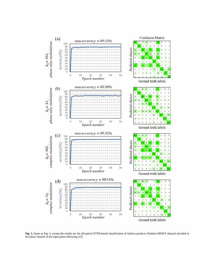
Fig. 3. Same as Fig. 2, except the results are for all-optical D2NN-based classification of fashion products (Fashion-MNIST dataset) encoded in

the phase channel of the input plane following [15].

Fig. 4. Classification accuracy, power efficiency and signal contrast comparison of MSE and SCE loss function based all-optical phase-only

D2NN classifier designs with 1, 3 and 5-layers. (a) Blind testing accuracy, (b) power efficiency and (c) signal contrast analysis of the final design of fully-connected, phase-only all-optical classifiers trained for handwritten digits (MNIST). (d-f) are the same as (a-c), only the classified dataset

is Fashion-MNIST instead.

Fig. 5. D2NN-based hybrid neural networks. (a) The architecture of a hybrid (optical and electronic) classifier. (b) Final design of phase-only

optical layers (𝛥𝑍 = 40 ) at the front-end of a hybrid handwritten digit classifier with a 10×10 opto-electronic detector array at the

bridge/junction between the two modalities (optical vs. electronic). (c) and (d) are same as (a) and (b), except the latter are for Fashion-MNIST dataset. Input plane represents the plane of the input object or its data, which can also be generated by another optical imaging system or a lens,

projecting an image of the object data onto this plane.

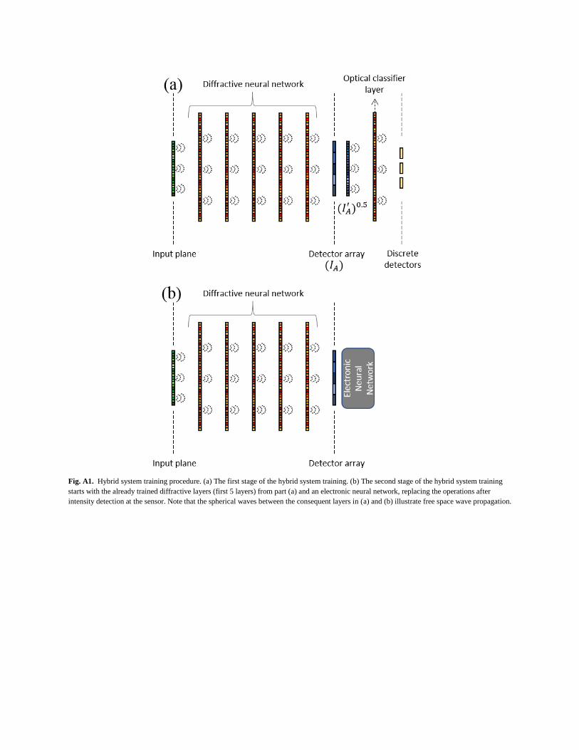
Fig. A1. Hybrid system training procedure. (a) The first stage of the hybrid system training. (b) The second stage of the hybrid system training

starts with the already trained diffractive layers (first 5 layers) from part (a) and an electronic neural network, replacing the operations after

intensity detection at the sensor. Note that the spherical waves between the consequent layers in (a) and (b) illustrate free space wave propagation.