Analysis of Differential Equations Applications from the ...
125
Brigham Young University BYU ScholarsArchive All eses and Dissertations 2017-08-01 Analysis of Differential Equations Applications from the Coordination Class Perspective Omar Antonio Naranjo Mayorga Brigham Young University Follow this and additional works at: hps://scholarsarchive.byu.edu/etd is esis is brought to you for free and open access by BYU ScholarsArchive. It has been accepted for inclusion in All eses and Dissertations by an authorized administrator of BYU ScholarsArchive. For more information, please contact [email protected], [email protected]. BYU ScholarsArchive Citation Naranjo Mayorga, Omar Antonio, "Analysis of Differential Equations Applications from the Coordination Class Perspective" (2017). All eses and Dissertations. 6502. hps://scholarsarchive.byu.edu/etd/6502
Transcript of Analysis of Differential Equations Applications from the ...

Brigham Young UniversityBYU ScholarsArchive
All Theses and Dissertations
2017-08-01
Analysis of Differential Equations Applicationsfrom the Coordination Class PerspectiveOmar Antonio Naranjo MayorgaBrigham Young University
Follow this and additional works at: https://scholarsarchive.byu.edu/etd
This Thesis is brought to you for free and open access by BYU ScholarsArchive. It has been accepted for inclusion in All Theses and Dissertations by anauthorized administrator of BYU ScholarsArchive. For more information, please contact [email protected], [email protected].
BYU ScholarsArchive CitationNaranjo Mayorga, Omar Antonio, "Analysis of Differential Equations Applications from the Coordination Class Perspective" (2017).All Theses and Dissertations. 6502.https://scholarsarchive.byu.edu/etd/6502

Analysis of Differential Equations Applications
from the Coordination Class Perspective
Omar Antonio Naranjo Mayorga
A thesis submitted to the faculty of Brigham Young University
in partial fulfillment of the requirements for the degree of
Master of Arts
Steven R. Jones, Chair Blake E. Peterson
Steven R. Williams
Department of Mathematics Education
Brigham Young University
Copyright © 2017 Omar Antonio Naranjo Mayorga
All Rights Reserved

ABSTRACT
Analysis of Differential Equations Applications from the Coordination Class Perspective
Omar Antonio Naranjo Mayorga Department of Mathematics Education, BYU
Master of Arts
In recent years there has been an increasing interest in mathematics teaching and learning at undergraduate level. However, many fields are little explored; differential equations being one of these topics. In this study I use the theoretical framework of Coordination Classes to analyze how undergraduate mechanical engineering students apply their knowledge in the context of system dynamics and what resources and strategies they used; in this subject, students model dynamics systems based on Ordinary Differential Equations (ODEs). I applied three tasks in different contexts (Mechanical, Electrical and Fluid Systems) in order to identify what information was relevant for the students, readout strategies; what inferences students made with the relevant information, causal nets; and what strategies students used to apply their knowledge in those contexts, concept projections. I found that the core problem at projecting their knowledge relied on the causal nets, coinciding with diSessa and Wagner’s conjecture (2005). I also identified and characterized three strategies or concept projections students used in solving the tasks: Diagram-based approach, Component-based approach and Equation-based approach.
Keywords: Coordination Class, Differential Equations, Transfer of Learning, Concept Projections

ACKNOWLEDGMENTS
I would like to express my gratitude to all the people who have helped me through
this wonderful adventure of writing my master’s thesis. I would like to thank my advisor,
Dr. Steven Jones for his immense patience, support and effective advice. I also express my
appreciation towards the members of my committee, Dr. Blake Peterson and Dr. Steve
Williams for their feedback. I would also like to thank my parents, my daughters and the
rest of my family and all the members of the BYU’s Mathematics Education Department for
their support and motivation. I would like to make special mention to Dr. Cheryl Garn for
her advice and support. Lastly, I would like to thank my wife Carolina; her wonderful
attitude and support have been a lighthouse in this journey and have uplifted my spirit
every time.

iv
TABLE OF CONTENTS
ABSTRACT ........................................................................................................................... ii
ACKNOWLEDGMENTS ..................................................................................................... iii
TABLE OF CONTENTS ...................................................................................................... iv
LIST OF FIGURES .............................................................................................................. vii
LIST OF TABLES ................................................................................................................ ix
CHAPTER 1: RATIONALE .................................................................................................. 1
CHAPTER 2: LITERATURE REVIEW ................................................................................ 8
Student Understanding of Differential Equations .............................................................. 8
Connections between Science/Engineering and Mathematics ......................................... 10
CHAPTER 3: THEORETICAL FRAMEWORK ................................................................ 13
Coordination Classes ........................................................................................................ 13
Readout Strategies and Causal Nets ................................................................................. 15
Transfer, Span, and Concept Projection ........................................................................... 16
Differential Equations and Coordination Classes ............................................................. 20
CHAPTER 4: METHODS ................................................................................................... 22
Participants ....................................................................................................................... 22
Instruments ....................................................................................................................... 23
Selection of Participants ................................................................................................... 25
Description and Solution of Task 1 .............................................................................. 26

v
Description and Solution of Task 2 .............................................................................. 30
Description and Solution of Task 3. ............................................................................. 33
Potential Readouts and Causal Nets ............................................................................. 35
Interviews ......................................................................................................................... 41
Data Analysis .................................................................................................................... 42
Stage One ...................................................................................................................... 43
Stage Two ..................................................................................................................... 44
Stage Three ................................................................................................................... 45
Pilot Study ........................................................................................................................ 45
CHAPTER 5: RESULTS ..................................................................................................... 48
Analysis of Students’ Answers to the Survey .................................................................. 48
Analysis of Students’ Written Work for Task 1 ............................................................... 51
Task 1 - Zane ................................................................................................................ 51
Task 1 – Rebecca .......................................................................................................... 58
Task 1 – Harry .............................................................................................................. 63
Task 1 - Josh ................................................................................................................. 66
Task 1 - Kira ................................................................................................................. 70
Summary of the Strategies ............................................................................................ 74
Analysis of Students’ Written Work for Task 2 ............................................................... 75
Task 2 – Zane ............................................................................................................... 75
vi
Task 2 – Rebecca .......................................................................................................... 78
Task 2 – Harry .............................................................................................................. 81
Task 2 – Josh ................................................................................................................ 83
Task 2 – Kira ................................................................................................................ 85
Analysis of Students’ Written Work for Task 3 ............................................................... 88
Task 3 – Zane ............................................................................................................... 88
Task 3 – Rebecca .......................................................................................................... 91
Task 3 – Harry .............................................................................................................. 94
Task 3 – Josh ................................................................................................................ 96
Task 3 – Kira ................................................................................................................ 98
Summary of Results ....................................................................................................... 100
CHAPTER 6: DISCUSSION ............................................................................................. 102
Implications for the Coordination Class Theory ............................................................ 102
Students’ Leaning on Mathematical Concepts ............................................................... 104
Students’ Strategies as Concept Projections ................................................................... 105
Learning Differential Equations ..................................................................................... 107
Understanding of Students’ Thinking of Differential Equations.................................... 108
Implications for Transfer of Learning Processes ............................................................ 109
Conclusion ...................................................................................................................... 109
REFERENCES ................................................................................................................... 111
vii
LIST OF FIGURES
Figure 1. Connection between physics, mathematics and system dynamics. ...................... 11 Figure 2. “Bird”and “Force”concepts. ................................................................................. 13 Figure 3. Preliminary survey. ............................................................................................... 24 Figure 4. Task 1. .................................................................................................................. 27 Figure 5. Free body diagram of the pendulum. .................................................................... 27 Figure 6. Task 2. .................................................................................................................. 30 Figure 7. Task 3. .................................................................................................................. 33 Figure 8. Mechanical system for the pilot study. ................................................................. 47 Figure 9. Analysis of a student’s work in a pilot study. ....................................................... 47 Figure 10. Zane’s initial excerpts from his work on Task 1. ............................................... 52 Figure 11. Zane’s Free Body Diagram of the Pendulum. .................................................... 53 Figure 12. Zane’s ODE. ....................................................................................................... 54 Figure 13. Zane’s final expression. ...................................................................................... 54 Figure 14. Zane’s flow of reasoning for task 1. ................................................................... 57 Figure 15. Rebecca’s identification of Newton’s Second Law for Task 1. ......................... 59 Figure 16. Rebecca’s partial ODE. ...................................................................................... 60 Figure 17. Rebecca’s component-based analysis of the system. ......................................... 60 Figure 18. Rebecca’s final ODE. ......................................................................................... 61 Figure 19. Rebecca’s flow of reasoning for task 1............................................................... 62 Figure 20. Harry’s misinterpretation of the pendulum inertia. ............................................ 64 Figure 21. Harry’s partial setting up of the ODE. ................................................................ 64 Figure 22. Harry’s final ODE. ............................................................................................. 64 Figure 23. Harry’s flow of reasoning for task 1. .................................................................. 66 Figure 24. Josh first attempt to make sense of the system’s behavior. ................................ 67 Figure 25. Josh’s preliminar expressions. ............................................................................ 67 Figure 26. Josh’s final expression. ....................................................................................... 68 Figure 27. Excerpt from Josh’s discussion about ODE solution techniques. ...................... 69 Figure 28. Josh’s flow of reasoning for task 1. .................................................................... 70 Figure 29. Kira’s FBD. ........................................................................................................ 71 Figure 30. Kira’s reasoning about the components of the system from the equations. ....... 72 Figure 31. Kira’s final ODE. ................................................................................................ 73 Figure 32. Kira’s flow of reasoning for task 1. .................................................................... 73 Figure 33. Zane’s drafts for Task 2. ..................................................................................... 77 Figure 34. Zane’s flow of reasoning for task 2. ................................................................... 77 Figure 35. Rebecca’s initial work on Task 2........................................................................ 78 Figure 36. Rebecca’s diagram of the circuit. ....................................................................... 79 Figure 37. Rebecca’s final expression. ................................................................................ 79 Figure 38. Rebecca’s flow of reasoning for task 2............................................................... 81 Figure 39. Harry’s evidence of KCL use. ............................................................................ 82 Figure 40. Harry’s final expression (ODE). ......................................................................... 82 Figure 41. Harry’s flow of reasoning for task 2. .................................................................. 83 Figure 42. Josh’s final expression. ....................................................................................... 84 Figure 43. Josh’s flow of reasoning for task 2. .................................................................... 85

viii
Figure 44. Kira’s component-based approach results. ......................................................... 86 Figure 45. Kira’s flow of reasoning for task 2. .................................................................... 87 Figure 46. Zane’s analogies between systems. .................................................................... 88 Figure 47. Zane’s guiding (Bernoulli) equation. .................................................................. 88 Figure 48. Exclusion of compressibility term from Zane’s equation. .................................. 88 Figure 49. Zane’s preliminary equation to obtain the ODE. ................................................ 89 Figure 50. Zane’s ODE for Task 3. ...................................................................................... 90 Figure 51. Zane’s flow of reasoning for task 3. ................................................................... 91 Figure 52. Rebecca’s preliminary equation excluding the 4th term. ................................... 92 Figure 53. Rebecca’s final ODE for task 3. ......................................................................... 92 Figure 54. Rebecca’s flow of reasoning for task 3............................................................... 93 Figure 55. Harry’s final ODE for task 3. ............................................................................. 95 Figure 56. Harry’s flow of reasoning for task 3. .................................................................. 95 Figure 57. Josh’s flow of reasoning for task 3. .................................................................... 97 Figure 58. Kira’s final ODE for task 3 and qout interpretation. ............................................ 98 Figure 59. Kira’s flow of reasoning for task 3. .................................................................... 99

ix
LIST OF TABLES
Table 1 .................................................................................................................................. 29 Table 2. ................................................................................................................................. 35 Table 3. ................................................................................................................................. 36 Table 4. ................................................................................................................................. 38 Table 5. ................................................................................................................................. 38 Table 6. ................................................................................................................................. 40 Table 7. ................................................................................................................................. 41 Table 8. ................................................................................................................................. 50 Table 9. ............................................................................................................................... 101 Table 10. ............................................................................................................................. 101

1
CHAPTER 1: RATIONALE
In this study, I intend to explore how students apply the concepts learned in ordinary
differential equations (ODE) courses in the context of an advanced engineering subject, “System
Dynamics”. In this chapter, I provide the justifications for carrying out this study as well as its
importance for both the mathematics education and engineering education communities.
First, I wish to speak of two separate, but related issues within mathematics education. On
one hand, there has been a growing need for professionals in degrees related to Science,
Technology, Engineering and Mathematics (STEM) to help in improving and maintaining the
economic competitiveness of the U.S. with respect to technological and scientific capabilities
(Matthews, 2007; Hall et al, 2011; NMS, 2014; Peters and Kortecamp, 2010). In fact, any
country interested in keeping its industrial, scientific and economic pace has a commitment to
promote the STEM structure that supports it. From the different fronts from which the STEM role
can be strengthened, one is through focusing efforts on improving STEM instruction at all
academic levels (PCAST, 2012).
On the other hand, the educational problems faced by high school and college level
students present various challenges for mathematics education researchers. Matthews (2007)
emphasized the importance of making the necessary arrangements so that the parties involved
(schools, universities, and governmental institutions, among others) pay special attention to the
decline of students choosing STEM related programs at university level (Chen and Soldner,
2013; NMS, 2014). Furthermore, Martinez and Sriraman (2015) also pointed at a fact that many
of those who are currently doing STEM degrees face several challenges along the process and
choose to leave. One of their findings involves the quality of mathematics instruction at

2
undergraduate and graduate level and how it might be one of the causes of STEM students’
attrition.
In this way, on one hand there are STEM students’ attrition and the necessity of recruiting
more students to study STEM related degrees for the reasons aforementioned. On the other hand,
for years, there have been concerns about the teaching and learning process at university level.
One of the reasons for this concern implies the need for preparing future engineers and scientists
for today’s world’s challenges. Hence, research has turned its attention to this issue in recent
decades.
Several studies have addressed issues related to teaching and learning mathematics at the
University level (Artigue, 1999; Peters and Kortecamp, 2010; Bergsten, 2007; Wainwright and
Flick, 2007). As the number of students attending universities increased, it was necessary to pay
attention to educational issues at this level of mathematics. Studies at this level include: The
conceptualization of calculus topics and the conciliation between what is taught at high school
and what students should “know” when starting college level mathematics (Pilgrim, 2014;
Artigue, 1999); Notions and conceptions of limits (Shipman, 2012; Güçler, 2012), derivatives
(Hashemi, et al, 2015; Orton, 1983), definite integrals (Jones, 2015a) , integrals of other kinds
(Jones, 2015b), proof (Powers et al, 2010), differential equations (Soon et al, 2011; Rasmussen,
2001), and linear algebra (Celik, 2015). The amount of specific studies about mathematics at this
level is evidence that there are significant issues that demand the attention of the mathematics
education researchers, along with science and engineering education researchers.
Of the undergraduate mathematics education foci, one emerging branch is concerned with
connections between mathematics and other STEM disciplines, such as science and engineering.
Furthermore, the European Society for Engineering Education (SEFI, 2013) issued a framework
3
for mathematics curricula in engineering education with the intention of making a contribution to
the improvement and development of higher engineering education. Out of the several
recommendations presented, the SEFI Mathematics group quoted Willcox and Bounova (2004):
One of the major findings of this study was that the engineering faculty is unaware of the
details of mathematics class curricula – they do not know specifically where and how
mathematical concepts are taught. Likewise, for many concepts, mathematics faculty do
not have a clear understanding of precisely how their downstream “customers” will use
the skills they teach (Willcox and Bounova, 2004, p. 9)
This statement evidences a possible cause for the challenges that undergraduate
engineering students face at using their mathematics knowledge when they deal with
engineering-related tasks. As a consequence, this situation might generate a disconnect between
mathematics and applied sciences. Eventually, the effects will likely be evidenced in the
professional practice. This problem then, requires a concomitant effort from both engineering
education and mathematics education researchers if we are to deal with this issue more
efficiently. Booth (2008) addressed this issue of teaching and learning mathematics for an
engineering context, thinking about a future “knowledge society” which he defines as the new
societal paradigm that focuses its educational trend towards the necessities of our evolving
society; that is, the paradigm has moved from a humanistic, then industrial to a now modern view
that emphasizes creativity, resourcefulness, problem-solving skills among others. He presented
the results of three studies that shed some light as to how mathematics are used and what the
quality of their learning outcomes is, thinking about their future encounters with math-related
science/engineering/technology subjects. As part of the conclusions, Booth presented the
implications for the processes of teaching that provided the basis of students’ future skills and
4
how mathematics could be integrated in other aspects of their practice as students but also as
future professionals. In summary, “knowledge capability” and preparation for working in the
knowledge society comprise Booth’s conclusions. This implies that instruction should be aimed
at preparing engineers to be able to use their skills in an ever-evolving society in part by taking
their mathematical knowledge in their everyday contexts.
The problem of strengthening the connection between mathematics and applied sciences
can be seen from several points of view. Thus, it is important to illustrate a brief account of what
has been done in this respect in order to provide a proper reasoning of the objective of the present
study. Dray and Manogue (2004) pointed at the necessity of bridging the gap between
mathematics and physical sciences at college level, they referred to the importance of a correct
interpretation (and reconcile) symbolization to facilitate physics concepts understanding
involving mathematical principles. Horwitz and Ebrahimpour (2002) reported on a two-year
project including science and engineering projects in calculus (differential and integral) courses
in which two calculus classes worked on a project-basis framework with the intention of
achieving a stronger connection of the mathematical concepts and some contexts (engineering) in
which these could be applied. Though not necessarily successful, the project was focused on
making the connections more apparent. On the other hand, Pennell, et al., (2009) reported on a
program that intended to reinforce the connection between the concepts of differential equations
and the engineering practice. From among these lines of research, I will focus on how differential
equations concepts are applied in novel contexts by undergraduate students, specifically, at the
analysis of the application of differential equations concepts in engineering settings.
There is a strong notion of how mathematics and physics-related –or engineering-
subjects are interconnected, especially when it comes to interpreting notations or the way

5
physical ideas and concepts are mixed with the mathematics concepts. For example, the
mechanics of materials engineering course (Hibbeler, 1997) has a high load of calculus concepts
such as derivatives, rates of change, and integrals. There are also concepts from geometry and
algebra, fluid mechanics (Fox, 2011), heat transfer (Incropera, 2007), thermodynamics (Çengel,
2002) and system dynamics (Palm, 2005). In this way, mathematics becomes an essential element
that enhances the understanding but it is not the only component needed to perform tasks in
physics or advanced engineering/science topics. However, when a student cannot clearly
understand certain critical mathematical concepts, he/she may find extreme difficulties going any
further with engineering or science task involving mathematical concepts. This problem can also
be given the other way around, that is, the lack of understanding of physical concepts may
prevent the possibility to model real life situations using mathematical tools. Eventually this
might become an issue for the prospective professional who needs to make use of as many tools
as possible to be able to solve everyday problems at work.
Taking into account the last paragraph, one might argue about the specific kind of
knowledge that a professional – practicing – engineer should consider in his or her everyday
practice. Ellis et al., (2004) made a survey among 96 engineers who responded to a varied set of
questions regarding the (mathematical) conceptual understanding required of them at work,
focused on calculus knowledge. In particular, 66% of the interviewees asserted that they were
required to possess a conceptual understanding of differential equations. These results are
remarkable for this study in particular, since there is emphasis on what concepts engineers require
in their practice.
With this in mind, I have noticed the importance of the instruction provided in differential
equations courses and the influence it might exert on later settings where students are required to

6
use concepts learned from this subject. While there have been several studies that analyze how
students learn ODEs (Rassmussen, 2001; Arslan, 2009), what aspects influence this learning
(Raychaudhuri, 2013), and alternative strategies to help them have a better understanding
(Budinski, 2011; Rassmussen and Kwon, 2007; Savoye, 2009; Kwon, 2002), not much has been
studied as for what happens afterwards; namely, how students apply or use the ODEs concepts in
further stages of their instructions to become professionals. As it has been mentioned before,
differential equations concepts are often used in certain settings of professional engineers and
scientists so it is of great interest to dig into the complexities involving students transfer of
learning from a mathematics education research perspective.
The aforementioned studies provide a general perception of the concerns of researchers in
understanding the challenges involving the use of ODEs for future professionals. However,
within this intersection between mathematics and engineering education there are still gaps that
need exploring. Thus, this master’s thesis is intended to answer the following research question:
What knowledge resources and strategies do students use while setting up ODEs in these
engineering contexts?
Having personally graduated as a mechanical engineer, from my point of view I consider
that being able to apply ODEs to engineering is a matter of great importance. I expect to find
valuable information regarding the students’ process of thinking in transferring their knowledge.
As such, this study can contribute to both the mathematics and engineering education
community.
With the purpose of providing answers to the research questions, the aim of this thesis
entails choosing a specific engineering subject extensively connected with ODEs and analyzing
the way that undergraduate engineering students apply those concepts to the novel context. This

7
novel context is System Dynamics, a subject that mechanical engineering undergraduates have to
take usually a year or less before they graduate, so its relevance is evident as for assessing the
preparation of the future professional engineering graduate.
8
CHAPTER 2: LITERATURE REVIEW
Student Understanding of Differential Equations
In this section, I review the undergraduate education research literature pertaining to the
topic of differential equations. In particular, Rasmussen et al., (e.g., 2001, 2000), has conducted
several important studies about students’ understandings and difficulties regarding ODEs. The
objective for those studies was to explore the variety of ways by which elements, like content,
instruction and technology, can foster student learning. At the same time introducing a
framework within which researchers could be based to study the understanding, conceptualizing
and application of ODEs concepts.
Rasmussen’s (2001) framework presents two major themes: 1) functions-as-solutions
dilemma and 2) Students’ intuitions and images. These themes are presented as a way to interpret
students’ thinking. On the one hand, the first theme is divided into three subcategories: 1a)
Interpreting solutions 1b) Interpreting equilibrium solutions and 1c) Focusing on quantities.
These subsets can be interchangeably present at the moment a student is interpreting a system
represented by a differential equation; that is, what seems relevant to the student in order to show
his/her understanding. On the other hand, the second theme is also divided in three subtopics of
understanding: 2a) Equilibrium solutions, 2b) Numerical approximations and 2c) Stability.
The way students focused on the differential equations to interpret their solutions gave
Rasmussen the resources to build his framework. In this way, his study might serve as a useful
foundation to help understand how students in the present study might interpret the solution to
the proposed exercises. However, there are two topics that might not be covered at this point: 1)
Most of Rasmussen’s framework is based on first-order differential equations with only few
mentions to second-order differential equations. In this respect, the present study might shed

9
some light as for alternative ways of students’ interpretations. On the other hand, 2) Rasmussen’s
framework did not include how the context of the situation presented might influence the
interpretation of the solution of the differential equation, which plays a fundamental role in the
present study.
Also, Hubbard (1994) listed several characteristics of an ODE that imply its
understanding: 1) Understanding that the solution of a differential equation involves a function
and not a number; in fact, many possible solutions (functions) depending on the conditions. 2)
Present a description of how the solutions behave.
A differential equation describes the evolution of a system. Mental pictures of a differential
equation allow guesses about the system’s behavior. Also, there is a need to recognize the
elements and how these affect the behavior of the system. For example, consider the non-
homogenous, second-order differential equation:
i.e.: 0.1
A discussion about this system might include the recognition of it being a damped, non-
linear pendulum, forced system. It could also include an explanation of what happens to the
systems as the parameters change. For example, will forcing kick the bob over? What about the
friction? Is friction large enough to eventually make it stop?
Hubbard emphasizes on the necessity that the student communicates his/her findings or
conjectures in terms of statements and not merely in terms of formulas or numbers. For example,
how they describe the behavior of the system and what elements of the equation they use to
support their reasoning.
These are elements that facilitate a proper description of what the differential equation represents
given a certain context. However, it is also necessary to take into account the requirements of the

10
System Dynamics course in order to complement the analysis of a system. Palm (2005) states that
the objective of a system dynamics course entails the mathematical modeling and analysis of
devices and processes so that we understand its time-dependent behavior. In other words, it is
expected to predict the performance of a system as a function of time.
Connections between Science/Engineering and Mathematics
In this section, I address in more detail the literature regarding the connection between
science/engineering and mathematics. For example, Redish (2005) described mathematics as an
essential component for physics problem solving. Indeed, Redish discussed the issue of what
students thought they were doing while solving physics problem situations and how they applied
or used mathematical concepts in contrast with what instructors expected them to be doing. For
instance, when blending mathematics and physics, equations were interpreted in different ways
which caused discrepancies in many cases in the end results. Thus, it may be that this idea can be
extrapolated to other contexts, such as ODEs and its applications, revealing similar disparities.
It is possible to illustrate this matter with the following example. The equations shown
below describe a typical example of an ordinary differential equation. However, while equation
(1) might be the usual representation of the differential equation in a mathematics context, it is
possible to find representations like the one presented in equation (2) in settings such as
engineering classes. Though it might be considered a simple issue, its implications have been
described by Dray and Manogue in reference to ambiguous interpretations of mathematics and
physics on the concept of functions and their use in physics as quantities (2004), and the way
mathematicians, on one hand, and scientists and engineers, on the other, interpret vector calculus
(2003). This issue suggests that the lack of understanding might prevent an appropriate
application of the concepts taken from the mathematics practice, differential equations in

11
particular, or it might happen the other way around. That is, when applying physics or science
concepts to set up mathematical models that will ultimately serve as tools to understand the
behavior of dynamics systems involving differential equations. This leads to the question of how
one’s mathematical background affect this transfer process as an undergraduate student explores
engineering contexts involving the use of ODEs? What aspects (elements of previous knowledge)
are relevant when he/she transfers such concepts in that novel (engineering) situation?
0 (1)
0 (2)
Figure 1 shows a diagram that represents in brief the concepts that a student has to take
into account in order to perform system dynamics tasks. There is a wide variety of concepts from
the mathematics branch, calculus in particular, and these are mixed with knowledge from physics
and introductory engineering courses. This flow diagram displays the correlation between ODEs
and system dynamics and evidences the close connection between these two topics subject of the
present study.
Figure 1. Connection between physics, mathematics and system dynamics.

12
In summary, Rasmussen and Hubbard have studied students’ understanding of ODEs
concepts. The former established a framework to understand and categorize students’ thinking
focused on the different ways students interpret differential equations; the latter argues on the
necessity to establish aspects by which it is possible to evaluate whether a student actually
understands the concepts implied in a differential equation. Redish on the other hand, addressed
the use of mathematics in science/physics. In this study, I intend to explore students’ application
of differential equations concepts to model engineering systems. The applications of ODEs
involve two parts: The first entails modeling a system by obtaining an expression (ODE) and the
second part dealing with the understanding and process of finding the solutions of differential
equations. Since the second part has been more heavily addressed, in this study I focus on the
first part of the application process.
This first part of the process; that is, modelling of systems using differential
equations, is a topic that seems to have been little explored in the literature of mathematics and
engineering education. In this study I intend to delve into the process by which a student has to
set up the differential equation that describes a system in different contexts. I expect to obtain
relevant information that sheds light on this branch of mathematics that connects with
engineering since we currently do not have much knowledge in this respect. In brief, the
modelling process can be divided into three steps according to Blanchard (1998), (1) Establishing
the rules or laws that describe the relationships between the quantities to be analyzed. (2)
Defining the variables and parameters to be used in the model. (3) Using those relationships
between quantities to obtain the desired equation(s), an ODE in this case. This study attempts to
contribute to the existing literature by analyzing how students set up ODEs as they follow these
steps.
13
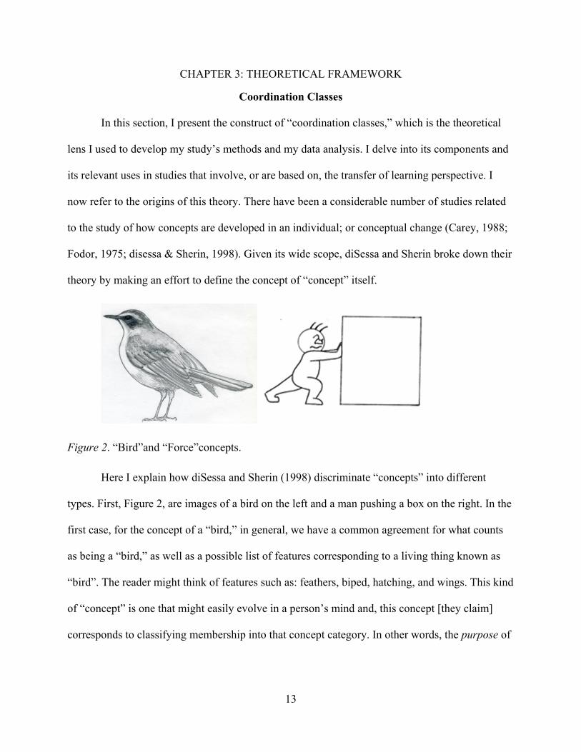
CHAPTER 3: THEORETICAL FRAMEWORK
Coordination Classes
In this section, I present the construct of “coordination classes,” which is the theoretical
lens I used to develop my study’s methods and my data analysis. I delve into its components and
its relevant uses in studies that involve, or are based on, the transfer of learning perspective. I
now refer to the origins of this theory. There have been a considerable number of studies related
to the study of how concepts are developed in an individual; or conceptual change (Carey, 1988;
Fodor, 1975; disessa & Sherin, 1998). Given its wide scope, diSessa and Sherin broke down their
theory by making an effort to define the concept of “concept” itself.
Figure 2. “Bird”and “Force”concepts.
Here I explain how diSessa and Sherin (1998) discriminate “concepts” into different
types. First, Figure 2, are images of a bird on the left and a man pushing a box on the right. In the
first case, for the concept of a “bird,” in general, we have a common agreement for what counts
as being a “bird,” as well as a possible list of features corresponding to a living thing known as
“bird”. The reader might think of features such as: feathers, biped, hatching, and wings. This kind
of “concept” is one that might easily evolve in a person’s mind and, this concept [they claim]
corresponds to classifying membership into that concept category. In other words, the purpose of

14
the concept is to define membership into that concept. The evolution of that concept happens as
the individual adds [or rejects] characteristics that make an entity “a bird”.
The picture showing the man pushing the box might be interpreted as one in which there
is a force involved – generated by the man – acting on the box being moved. This specific type of
concept involves a more than a membership classification. In other words, the “force” concept is
not necessarily just concerned with whether something belongs to the “force” concept, but is
more concerned with obtaining information about the force. The force is not directly visible by
an observer, unlike the bird that is directly visible, but must be inferred through related
observation, such as the acceleration of the object. The concept of “force” can be classified in the
type of concepts defined by diSessa and Sherin (1998) as coordination class. In this case, “force”
does not necessarily have a given visual prototype like there might be one for the concept of
“bird,” which helps distinguish whether an object is a bird or not. The purpose of the “force
concept” is to determine information about the force, such as its direction and magnitude, rather
than to identify whether a thing is or is not a “force.” This concept may consist of a collection of
certain types (classes) of features and elemental pieces of knowledge that when properly
coordinated comprise a coordination class concept. In this example, the concept of force is
composed of other basic elements, which we use to get the desired information. From our
knowledge of Newton’s laws we usually define force as the product of mass and acceleration, F
= ma. Therefore, this concept coordinates three foundational concepts: (1) the mass of the box,
which is the measure of inertia or opposition of that body to be moved; (2) multiplication which
accounts for a successive summation of a given quantity; and (3) acceleration which is the rate of
change of velocity with respect to time. By identifying those sub-elements that make up a force
(mass and acceleration) we are spotting the fact that we need to measure a mass and a change of
15
velocity of a body in order to “find” the force acting on it, that is, how much force is being
exerted on that body.
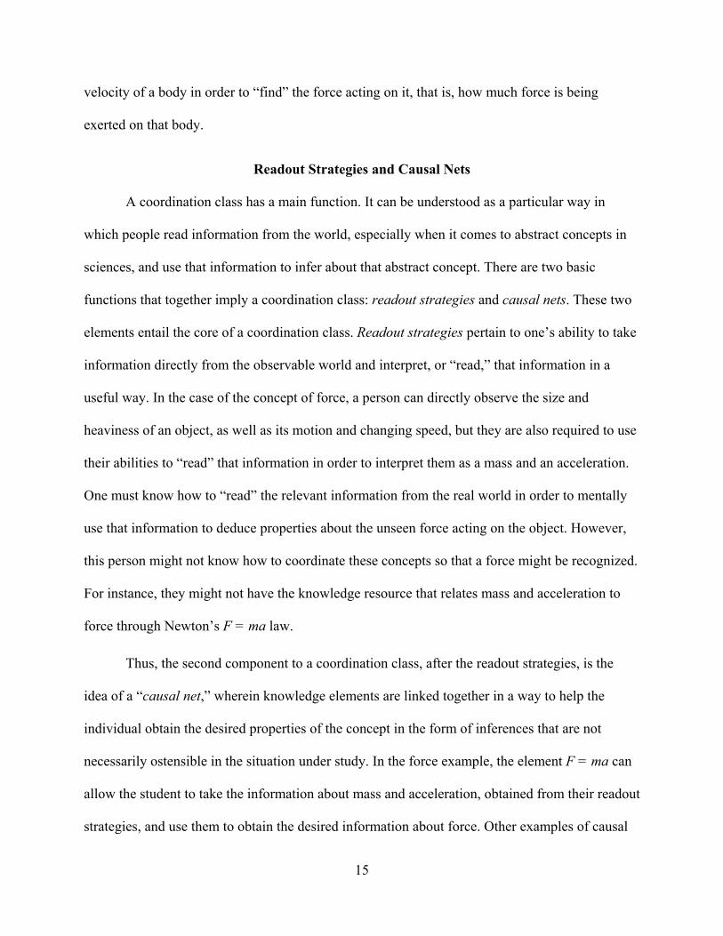
Readout Strategies and Causal Nets
A coordination class has a main function. It can be understood as a particular way in
which people read information from the world, especially when it comes to abstract concepts in
sciences, and use that information to infer about that abstract concept. There are two basic
functions that together imply a coordination class: readout strategies and causal nets. These two
elements entail the core of a coordination class. Readout strategies pertain to one’s ability to take
information directly from the observable world and interpret, or “read,” that information in a
useful way. In the case of the concept of force, a person can directly observe the size and
heaviness of an object, as well as its motion and changing speed, but they are also required to use
their abilities to “read” that information in order to interpret them as a mass and an acceleration.
One must know how to “read” the relevant information from the real world in order to mentally
use that information to deduce properties about the unseen force acting on the object. However,
this person might not know how to coordinate these concepts so that a force might be recognized.
For instance, they might not have the knowledge resource that relates mass and acceleration to
force through Newton’s F = ma law.
Thus, the second component to a coordination class, after the readout strategies, is the
idea of a “causal net,” wherein knowledge elements are linked together in a way to help the
individual obtain the desired properties of the concept in the form of inferences that are not
necessarily ostensible in the situation under study. In the force example, the element F = ma can
allow the student to take the information about mass and acceleration, obtained from their readout
strategies, and use them to obtain the desired information about force. Other examples of causal
16
net elements might be that the direction of acceleration is the same as the direction of the force,
or that multiple forces acting simultaneously only produce acceleration in a single direction
determined by the sum of the forces. There may even need to be causal net elements that help the
student know that size and heaviness of an object both feed into determining “mass,” which is
then subsequently used in the F = ma causal net element to infer about force. In this last example,
we can see that sometimes causal net elements may feed into further causal net elements, creating
a true “web,” or “net” (as the name is meant to imply), of knowledge pieces.
To further illustrate the ideas of readout strategies and causal nets, I give another example
described by diSessa and Sherin (1998) drawing from a more familiar context. Imagine a person
that is purchasing a flight ticket to travel somewhere. If that person wants to know how long it
takes for the plane to arrive at the destination, it is necessary to coordinate certain pieces of
information that are printed on the ticket. A readout strategy may consist of the recognition of the
departure and arrival times as important and relevant aspects to help him/her know the duration
of the flight. However, the cognitive operation required to actually know how many hours the
flight takes entails a further operation, invoking the causal net. In this example, the traveler
knows that it is necessary to obtain the difference between the departure and arrival times to
produce the flight duration. Also, the traveler should have knowledge about time zones which
feed into their ability to correct calculate flight duration that passes through time zones. The
person has to make a set of inferences from the readouts in order to convert that information into
new information, the one that is required. That set of inferences is the causal net.
Transfer, Span, and Concept Projection
At the beginning of this section I mentioned that the coordination class theory is related to
the process of transfer of learning. I now briefly define transfer of learning and its relation with
17
coordination class and then I discuss the elements that entail a coordination class. By the end of
the section, I extend the relation between transfer and coordination class.
Transfer of learning “entails the use (or reuse) of previous knowledge acquired in one
situation (or class of situations) in a ’new’ situation (or class of situations)” (diSessa & Wagner
2005, p. 122). Several studies have taken different approaches to transfer in an effort to show
evidence of this phenomenon. However, given the fact that there are different types of transfer
approaches, it is important to adopt a specific transfer lens that may be consistent with one’s
guiding theory on knowledge. diSessa and Wagner (2005) have outlined a particular view of
transfer that is compatible with the coordination class paradigm. Thus, naturally, it is this
orientation toward transfer that I adopt for my study, and I describe this particular view in this
section.
In order to describe this transfer lens, there are more components of the coordination class
theory to bring up and discuss. I use the concept of force once more to illustrate these additional
constructs. First, suppose a student sees a spring compressed between a person’s two hands. It is
possible that the student can conclude in this situation that there are enough elements to infer that
the spring is exerting a force against the person’s hands. This is because he/she reads the relevant
elements that entail the concept of force. That is, there is a mass, it is being moved by the spring
and the student recognizes the physical law behind this “force” known as Hooke’s law. However,
this same student might not recognize that if a body is submerged in a tank filled with water, this
water is exerting a force that pushes this body toward the surface. In this way, the range of
applicability of the concept is limited to one’s ability to recognize the existence of the concept in
certain contexts. This range of “applicability” of the concept is known as span and it is developed
as the learner accumulates experience and knowledge.
18
As the individual accumulates that experience and knowledge, all of these combine with
the development of skills like intuition, creativity and resourcefulness, they eventually expand
their span to include additional contexts. The way in which the coordination class theory
evidences the expansion of the span is known as alignment. This means that the individual is able
to recognize that the coordination class (the concept) works in the same way as it works in the
previous situations that they experienced in the past. It is worth noting the fact that the theory of
coordination class is also based on the Piagetian conception of knowledge construction
(constructivism) since the individual scaffolds his/her knowledge upon previously acquired
concepts.
There is an important aspect to coordination classes that explains the process of span
expansion and further alignment. diSessa (2004), and diSessa and Wagner (2005), describe the
collection of strategies and knowledge elements used by the individual to implement the concept
(coordination class) in particular contexts as a concept projection. If we think of the student who
is able to recognize a force in the spring-mass system but cannot do so in the context of the body
submerged in water, then it is possible to analyze and keep track of all the decisions, strategies,
inferences and knowledge elements that this student might employ in one context versus another
context For example, the strategies and knowledge pieces used to reason about force in the
spring context would consist of their concept projection of force in the spring context, and the
potential strategies and knowledge pieces used to reason about force in the submerged object
context would consist of their concept projection of force in the fluid context.
To further illustrate the construct of “concept projection,” I give here an example within
mathematics. To begin, consider the concept of the roots of a quadratic function, which is likely a
coordination class concept because it deals with obtaining information in addition to the simple
19
categorization of something as a “root” or not. In general, students may be introduced to this
topic by first being given a function in the factored form, such as:
2 1
In this case, the student “reads” each set of parentheses as a factor. They then use a causal
net element to recognize that any factor has to be equal to zero to make f(x) = 0. Then they
further employ a causal net element to produce a solution after setting each factor to zero.
Consequently the roots or solutions of the equation (x+2)(x-1) = 0 are x = -2 and x = 1. The
concept of “root” is put to work by these readouts and the causal net, which scaffold the strategy
of setting each factor equal to zero. Thus, taken together, these readouts, causal net elements, and
strategies form the concept projection of roots in the factored context. That combination of
knowledge and strategies led him/her to project the root concept and work on this task.
Now suppose the student sees another quadratic function, one that is not given in the
factored form but in the standard form:
2 5
The student might first read the expression as a trinomial (whether they imagine that word
or not), and then use a causal net element that associates trinomials with factoring. They might
try to factor the trinomial and notice that it is not possible to use integers to change the expression
to its factored form. After this realization, the student may switch strategy. They may invoke a
separate causal net element that associates trinomials with the quadratic formula. This leads to the
distinct strategy of using the quadratic formula to find the roots through the solutions to the
equation 2 5 0. This separate set of readouts, causal net elements, and strategies
makes up the concept projection of roots in the trinomial context. That is, in this case, the
concept is projected by using this other strategy, the quadratic formula.
20
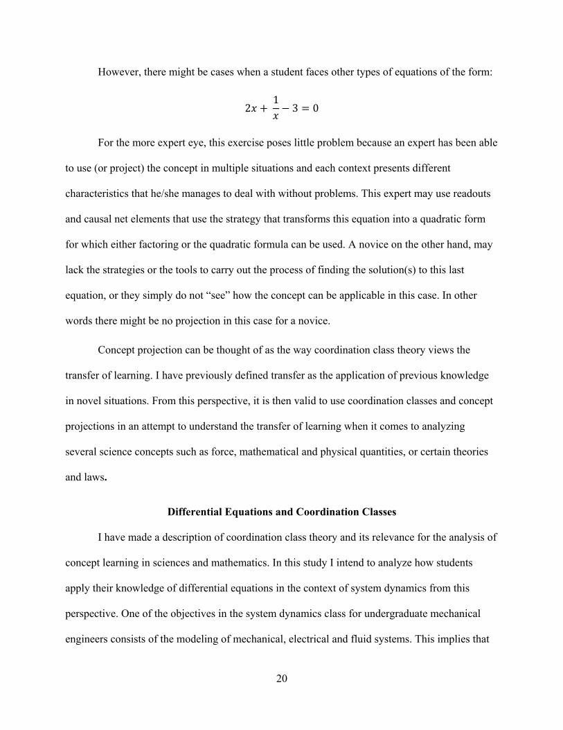
However, there might be cases when a student faces other types of equations of the form:
2 1
3 0
For the more expert eye, this exercise poses little problem because an expert has been able
to use (or project) the concept in multiple situations and each context presents different
characteristics that he/she manages to deal with without problems. This expert may use readouts
and causal net elements that use the strategy that transforms this equation into a quadratic form
for which either factoring or the quadratic formula can be used. A novice on the other hand, may
lack the strategies or the tools to carry out the process of finding the solution(s) to this last
equation, or they simply do not “see” how the concept can be applicable in this case. In other
words there might be no projection in this case for a novice.
Concept projection can be thought of as the way coordination class theory views the
transfer of learning. I have previously defined transfer as the application of previous knowledge
in novel situations. From this perspective, it is then valid to use coordination classes and concept
projections in an attempt to understand the transfer of learning when it comes to analyzing
several science concepts such as force, mathematical and physical quantities, or certain theories
and laws.
Differential Equations and Coordination Classes
I have made a description of coordination class theory and its relevance for the analysis of
concept learning in sciences and mathematics. In this study I intend to analyze how students
apply their knowledge of differential equations in the context of system dynamics from this
perspective. One of the objectives in the system dynamics class for undergraduate mechanical
engineers consists of the modeling of mechanical, electrical and fluid systems. This implies that
21
students are asked to determine the quantity to be studied and to obtain an expression (an ODE)
that relates that quantity with its derivatives. In other words, they have to design a model that
allows them to predict the system’s behavior with respect to time. In general, for this kind of
systems, the expression to be obtained is an Ordinary Differential Equation (ODE).
As described earlier, according to Blanchard et al (1998), the process of modeling consists
of three steps. The first step entails establishing the rules or laws that describe the relationships
between the quantities to be analyzed. The next step consists of defining the variables and
parameters to be used in the model. The third step is using those relationships between quantities
to obtain the desired equation(s), an ODE in this case.
The way that we can obtain information from a system is then given by the proper
modeling of it. Thus, coordination classes offer a suitable approach to analyzing the readout
strategies, causal nets, and possible concept projections evidenced by a student attempting to
work with differential equations in these engineering contexts. This is feasible especially because
the setting I investigate involves students who are taking a system dynamics course and all of
them have had the opportunity to take a differential equations course.
Most of the equations obtained by the students when modeling different types of systems
(mechanical, electrical and fluid, or a combination of these) follow the pattern of ordinary first or
second order differential equations. These can be homogenous or non-homogenous and linear or
non-linear. This engineering course excludes the use of partial differential equations because all
of the systems to study are time-dependent only. In this way, students are likely to set up
equations of the form. I describe this form, and how it relates to the contexts under investigation
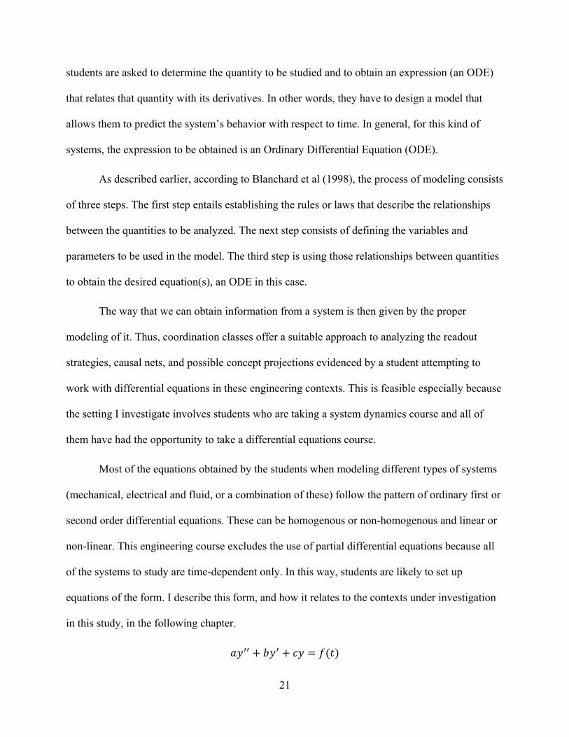
in this study, in the following chapter.
22
CHAPTER 4: METHODS
The arguments presented at the beginning of this study called for the necessity of
continuing with research focused on finding elements that contribute to the strengthening of the
teaching and learning process of mathematics in STEM contexts. As for this study, I emphasize
that the connection between mathematics and science and/or engineering is a matter that requires
attention from mathematics and engineering education as part of the potential solutions to
improve the learning and teaching of mathematics and engineering at undergraduate level,
promote STEM programs, deter students from detrition, among others.
In this study I intend to answer the questions posed in the introduction regarding how
students apply ODEs to engineering contexts involving system dynamics from a coordination
class perspective. This perspective influenced the design of the instruments of data collection,
organization and analysis. These are described in the following paragraphs.
Participants
The study included the participation of five undergraduate mechanical engineering
students. The participants were taking the system dynamics class offered by the mechanical
engineering department at the time of recruitment. These students had all already taken a
differential equations course, as it is a prerequisite for the system dynamics class.
In general, students at this stage are about to graduate and the topics they study during the
system dynamics course are likely to become part of the professional practice for some of them.
At this point of the program, the students have already taken the usual calculus series and also the
series of fundamentals of physics, as well as the first two courses of applied mechanics, statics
and dynamics, (see Figure 1 in the introduction). This helps to make sure that students have
enough background for the tasks to be applied during the sessions. For this manuscript, the five
23
students have been given the pseudonyms, Zane, Kira, Harry, Rebecca and Josh. All of them
were senior mechanical engineering undergraduates from a large university in the United States
and were taking the system dynamics class during the time of the interviews and volunteered to
take part of the study. They were chosen from among a group of 60 students based on their
responses to an initial survey, which I now describe. In the next section, I describe the procedure
for which I chose the participants in the study.
Instruments
In this section I describe the instruments I used to collect the information. Then, I explain
the process to choose the participants in the study and the tasks I assigned them during the
sessions I interviewed them. When describing the tasks assigned to the students I also show how
the tasks are solved and the aspects I took into account to be used during the data analysis stage
of the study.
The initial survey contained a set of questions regarding the student’s interpretation of the
elements comprising ODEs, as well as a section where they expressed their willingness to
participate in the study. I coordinated the administration of the survey with the professor in
charge of the System Dynamics class one month before the end of the semester.
The survey contained a set of six questions that asked the students to express what they
knew and how much they knew and understood about ordinary differential equations (ODEs).
The questions were focused on each of the elements of the ODE, including how they interpreted
the second derivative of y (y’’), the first derivative of y (y’), the function y, what the constants a,
b and c represent, and finally, what zero represents in the equation (see Figure 1). The reason
behind choosing this specific differential equation is because that model is typical in System
Dynamics settings. Thus, students will be reporting their knowledge about a differential equation

24
with which they should be acquainted at this stage of the study and, at the same time, one that is
closely related to the exercises that the interviewees dealt with eventually.
Figure 3. Preliminary survey.
I expected to recruit the five participants in the following way. I wanted two of them to be
students who would potentially show a high performance in solving the tasks, two of them to be
at a “medium” level, and one more student who might have difficulties with the subject. With
that in mind, I could have the possibility to find evidence for both advantages of certain strategies
and possible difficulties associated with the students’ concept projections of ODEs in the system
dynamics contexts.

25
Selection of Participants
Two of the participants were chosen on the basis of the clarity and accurate explanation of
the questions from the survey. These two students were able to give more details when answering
question 1, for example. Both explained the whys beyond correctly identifying it as a second
order linear homogeneous differential equation. These two students also provided clear
understanding of the meaning of each of the elements of the ODE along with examples of
applications in which these elements are used. In question 1 they explained that it is a second
order differential equation because the highest derivative in the expression is a second derivative,
that homogeneity implies that the ODE equals to zero which means that it has no forced input. In
contrast, one of the students considered to have challenges with the concepts, only explained that
it was a second order differential equation involving “two derivatives”. In question 5, they
identified the constants as parameters that affect the system when they take different values.
Also, from question 6, they showed understanding that when the equation is not equal to zero,
there is an external element, in the form of a function that affects the system, also known as
forced response.
The other three participants had a fair understanding of what the differential equation was.
They demonstrated reasonable understanding from part (a) of each question, but for part (b) they
either lacked information about the representation of each element, or their response was actually
irrelevant to the question. In the case of the student who I predicted to have a poor performance,
the answers were short, inaccurate and/or irrelevant. This participant barely identified the
elements of the ODE and showed little depth in the responses. For example, in question 6, this
participant was limited in her response: “no input of force [if it equals to a value other than zero]
turns it into a step or forced response”. In this case, this student immediately correlates the

26
equation with a system of forces not showing evidence that these quantities could be of different
nature, a limited applicability of the concept. We can compare it with the response of a high-
performing student who replied: “There is no forcing function of input… [if it equals to a value
other than zero] the ODE has a forced response in addition to the free response”.
As I analyzed the surveys, I selected ten students, divided in two groups, who satisfied the
profiles described in the previous paragraph. One main group and the second acted as a backup. I
contacted the participants through email and by phone and invited them to participate in two 45-
minute sessions approximately. One student from the main group did not reply so I picked the
replacement from the back-up group. For the interviews, I used three tasks that were similar to
exercises they had seen and done in their system dynamics class. In order to have various
contexts to work with, I chose a mechanical system task, an electrical system task, and a fluid
system task. The students were asked to set up a differential equation that modeled each of the
systems. In order to provide the reader with a baseline of what each task involved, in the
following subsections I describe each of the three tasks the students were given, as well as a
complete “expert-view” solution of them.
Description and Solution of Task 1
Figure 4 shows the first task given to the students in the interviews, which can be
considered a fairly routine, though non-trivial, task for the students in this class. Here I give a
conceptual analysis of this task. The pendulum’s swing will be affected by the elements
connected to it. Furthermore, since it is a pendulum, those elements will make it rotate about the
center of rotation shown between and . This fact implies that the ODE will be generated
from the summation of moments in the system, where a moment is the product of force times the
distance from the center of rotation. A Free Body Diagram can be a useful tool to describe the

27
effect of each element in the system’s behavior. In Figure 5, the pendulum is influenced by three
different forces produced by the elements in the system: the force caused by Spring 1(k1) on top,
and force exerted by the Spring 2 (k2) and the damper (Fc).
Figure 4. Task 1. (Taken from Palm, 2005, p. 244).
Figure 5. Free body diagram of the pendulum.
28
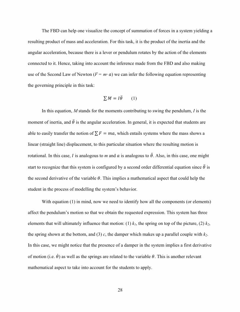
The FBD can help one visualize the concept of summation of forces in a system yielding a
resulting product of mass and acceleration. For this task, it is the product of the inertia and the
angular acceleration, because there is a lever or pendulum rotates by the action of the elements
connected to it. Hence, taking into account the inference made from the FBD and also making
use of the Second Law of Newton (F = m∙ ) we can infer the following equation representing
the governing principle in this task:
∑ (1)
In this equation, M stands for the moments contributing to swing the pendulum, I is the
moment of inertia, and is the angular acceleration. In general, it is expected that students are
able to easily transfer the notion of ∑ , which entails systems where the mass shows a
linear (straight line) displacement, to this particular situation where the resulting motion is
rotational. In this case, is analogous to m and is analogous to . Also, in this case, one might
start to recognize that this system is configured by a second order differential equation since is
the second derivative of the variable . This implies a mathematical aspect that could help the
student in the process of modelling the system’s behavior.
With equation (1) in mind, now we need to identify how all the components (or elements)
affect the pendulum’s motion so that we obtain the requested expression. This system has three
elements that will ultimately influence that motion: (1) k1, the spring on top of the picture, (2) k2,
the spring shown at the bottom, and (3) c, the damper which makes up a parallel couple with k2.
In this case, we might notice that the presence of a damper in the system implies a first derivative
of motion (i.e. ) as well as the springs are related to the variable . This is another relevant
mathematical aspect to take into account for the students to apply.
29
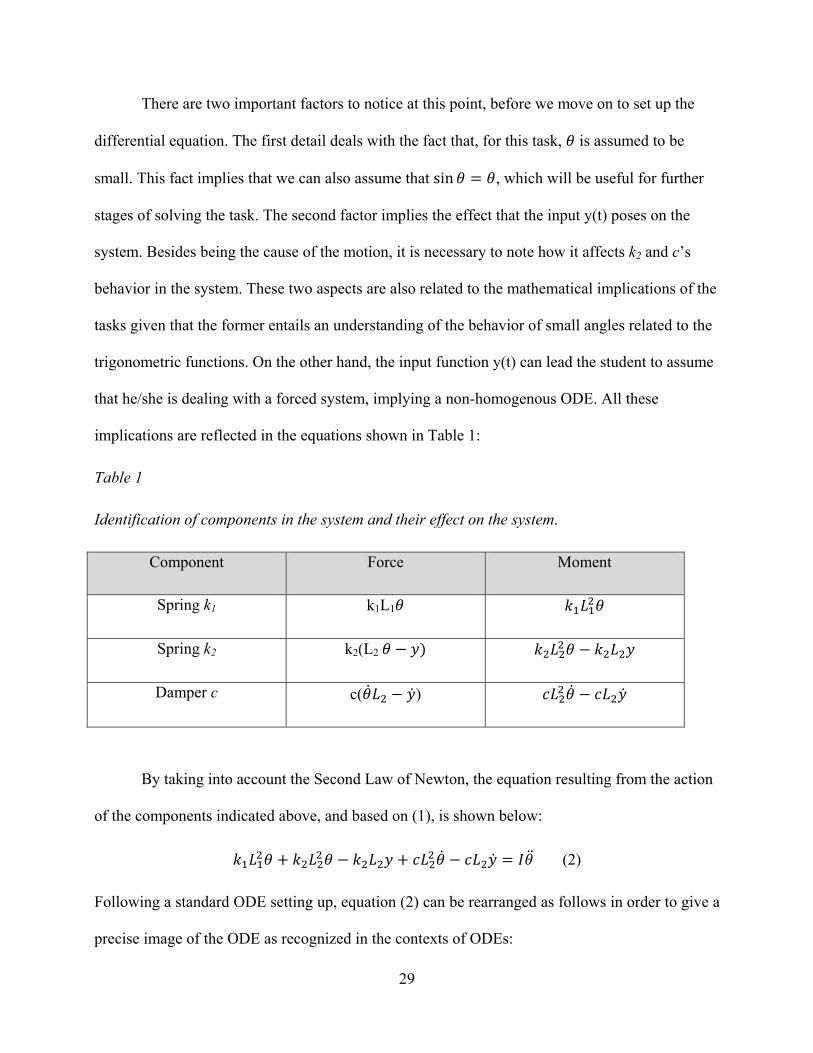
There are two important factors to notice at this point, before we move on to set up the
differential equation. The first detail deals with the fact that, for this task, is assumed to be
small. This fact implies that we can also assume that sin , which will be useful for further
stages of solving the task. The second factor implies the effect that the input y(t) poses on the
system. Besides being the cause of the motion, it is necessary to note how it affects k2 and c’s
behavior in the system. These two aspects are also related to the mathematical implications of the
tasks given that the former entails an understanding of the behavior of small angles related to the
trigonometric functions. On the other hand, the input function y(t) can lead the student to assume
that he/she is dealing with a forced system, implying a non-homogenous ODE. All these
implications are reflected in the equations shown in Table 1:
Table 1
Identification of components in the system and their effect on the system.
Component Force Moment
Spring k1 k1L1
Spring k2 k2(L2
Damper c c( )
By taking into account the Second Law of Newton, the equation resulting from the action
of the components indicated above, and based on (1), is shown below:
(2)
Following a standard ODE setting up, equation (2) can be rearranged as follows in order to give a
precise image of the ODE as recognized in the contexts of ODEs:

30
(3)
This expression contains the variable and its derivatives, the coefficients are all constant
and the right side of the equation shows the input function. This final expression for Task 1 is a
non-homogenous linear second order differential equation.
Description and Solution of Task 2
Figure 6. Task 2. (Taken from Palm, 2005, p. 372).
I now turn my attention to the second task given to the students in their interview (Figure
6), involving electrical systems the students were required to work with in the systems dynamics
class. I note that this particular task was the most difficult, and was used in order to see how
students might work with a rather challenging context. In this task, similar to Task 1, we might
notice that the voltage is affected by the influence of three elements: the capacitor (C), the
inductance (L) and the resistor (R). The current “flows” through the circuit and it does because
of the potential difference known as voltage. This voltage changes (decreases) as the current
passes through each of the elements of the circuit. It decreases until it reaches a value of 0. This

31
fact indicates that the measure of the voltage will be different depending on where the measure is
taken.
On the other hand, from the Kirchhoff’s Law of Current (KCL) we know that, at a given
node1 the current going to the node is equal to the current flowing out of it. The following
equation indicates how the KCL works for this circuit. Given the node located at the point where
is, we have:
(4)
Also, from Ohm’s law, we know can define as follows:
or (5)
We need to analyze and define the effect of the other two elements involved in the circuit.
In equation (5) we have already described the effect of the resistance on the system. Now we
describe the influence of the capacitor (C) on the system:
(6)
From equations (4) and (5) we can rearrange equation (6) as follows:
(7)
This is a significant aspect to take into account, mathematically speaking, given that this
term is part of the final expression. A student should be able to recognize that although this term
involves the variable to model, , it is necessary to derive it so that we eventually obtain the
ODE we are look for.
1 A node is a point on the circuit where two or more elements meet.
32
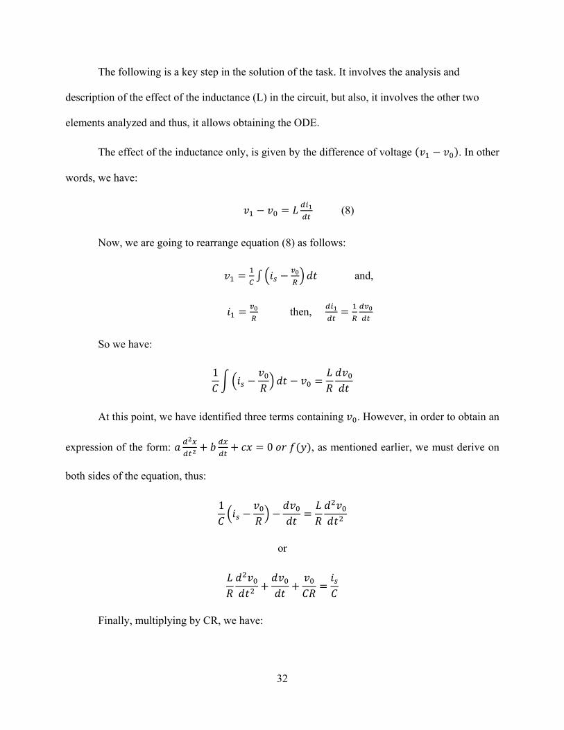
The following is a key step in the solution of the task. It involves the analysis and
description of the effect of the inductance (L) in the circuit, but also, it involves the other two
elements analyzed and thus, it allows obtaining the ODE.
The effect of the inductance only, is given by the difference of voltage . In other
words, we have:
(8)
Now, we are going to rearrange equation (8) as follows:
and,
then,
So we have:
1
At this point, we have identified three terms containing . However, in order to obtain an
expression of the form: 0 , as mentioned earlier, we must derive on
both sides of the equation, thus:
1
or
Finally, multiplying by CR, we have:

33
Similar to Task 1, we have obtained a linear second order differential equation with
constant coefficients. There is an input function, is, acting as the input function so this is a non-
homogenous ODE.
Description and Solution of Task 3.
Figure 7. Task 3. (Taken from Palm, 2005, p. 397-398)
I now discuss the third, and final, task given to the students during their interviews. I note
that this task, which involves a fluid context, was the easiest and was given to see how students
might work with a fairly uncomplicated context. This task requires the analysis of the section of
the tank that encompasses the height h, which is the magnitude of interest. In this way, the
volume of the tank in this section is given by the expression: . This volume V will vary
depending on the input and output flow ( and the orifice at L, respectively). The variation of
the volume (or rate of change) is given by the expression , or the derivative of V, thus we have:

34
This first aspect of the task entails the recognition of related rates of change, an important
topic in calculus. On the other hand, by determining the rate of change of the volume, we came
up with a derivative of the variable we are analyzing.
We can adapt Bernoulli’s equation to this tank situation. The Bernoulli’s principle
considers the conservation of energy in fluid systems. In brief, the rate of change of the volume
of volume flowrate is equal to the difference of the input and output flowrate:
(9)
From equation (9) we know we are close to obtain the model for h. The only term to
define is which relates the volume flowrate at the orifice at L.
2 (10)
Where is the discharge coefficient for the orifice, is the area of the orifice
and g is the gravity constant.
Now equation (9) can be rewritten as follows:
2 (11)
In this case we have obtained a non-linear first-order differential equation given that the
variable h is raised to the ½ power. At this point, students are not required to know the processes
to solve this kind of equations; however, they are expected to understand and recognize the
elements that make up this type of ODE.

35
Potential Readouts and Causal Nets
Now that I have presented an expert’s version of how the tasks could be solved, I provide
a list of likely readout strategies and causal net elements needed to solve each of the tasks. I
conceptualized of this list before performing the analysis, in order to have specific items to look
for during analysis, though, of course, I left open the possibility of detecting additional readouts
and causal net elements as well. In Table 2. I present the potential readouts strategies and causal
net elements of each task, one at a time. I give the symbols likely to be associated with the
readout or causal net element, the interpretation or association for each, and the code I use for
ease in referring to these readouts and causal net elements in the results section. This list of
readouts and causal nets for each of the tasks was contrasted with the work done by the students
and analyzed matches as well as missing aspects in their work compared with the expert’s solved
tasks.
Table 2.
List of potential readouts for task 1.
Task element Possible readout Code
y Input function that makes the system (pendulum)
to experience motion (Useful to obtain the expression to model the system behavior).
T1RO01
k2 Spring 2 constant (To calculate the force and eventually, the moment caused by spring 2)
T1RO02
c Damping constant (To calculate the force, and
eventually, moment caused by the damper)
T1RO03
L2 Distance from the point of rotation of the lever
(pendulum) (To calculate the moment caused by the elements attached to that end)
T1RO04
Amplitude of the pendulum caused by the elements
of the system. This is the variable that represents the output (t)
T1RO05
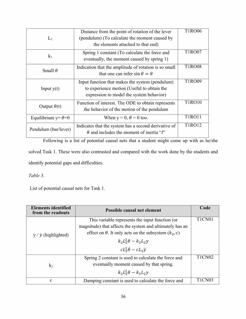
36
L1 Distance from the point of rotation of the lever
(pendulum) (To calculate the moment caused by the elements attached to that end)
T1RO06
k1 Spring 1 constant (To calculate the force and eventually, the moment caused by spring 1)
T1RO07
Small Indication that the amplitude of rotation is so small
that one can infer sin
T1RO08
Input y(t) Input function that makes the system (pendulum)
to experience motion (Useful to obtain the expression to model the system behavior)
T1RO09
Output (t) Function of interest. The ODE to obtain represents
the behavior of the motion of the pendulum
T1RO10
Equilibrium y= =0 When y = 0, = 0 too. T1RO11
Pendulum (bar/lever) Indicates that the system has a second derivative of
and includes the moment of inertia “I”
T1RO12
Following is a list of potential causal nets that a student might come up with as he/she
solved Task 1. These were also contrasted and compared with the work done by the students and
identify potential gaps and difficulties.
Table 3.
List of potential causal nets for Task 1.
Elements identified from the readouts Possible causal net element Code
y / (highlighted)
This variable represents the input function (or magnitude) that affects the system and ultimately has an
effect on . It only acts on the subsystem ( , )
T1CN01
k2
Spring 2 constant is used to calculate the force and eventually moment caused by that spring.
T1CN02
c Damping constant is used to calculate the force and T1CN03

37
eventual moment caused by the damper
It also indicates the existence of a first derivative
L2 Distance from the point of rotation of the lever
(pendulum), it is part of the calculation of the moments generated by the damper and spring 2
T1CN04
L1 Distance from the point of rotation of the lever
(pendulum), it is part of the calculation of the moment generated by the spring 1
T1CN05
k1
Spring 1 constant is used to calculate the force and eventually moment caused by that spring.
T1CN06
It indicates that the system rotates, hence the ODE is
composed by a number of expressions implying moments. There is a sum of moments
T1CN07
Small Indication that the amplitude of rotation is so small that
one can infer sin
T1CN08
Input y(t) Input function that makes the system (pendulum) to
experience motion (Useful to obtain the expression to model the system behavior)
T1CN09
Output (t) Function of interest. The ODE to obtain represents the
behavior of the motion of the pendulum
T1CN10
Equilibrium y= =0 When y = 0, = 0 too. T1CN11
Pendulum (bar/lever) Indicates that the system has a second derivative of and
yields the expression
T1CN12
The existence of many elements
Indicates that their effect on the rotation of the pendulum will be given by the summation of moments equal to the
product of the moment of inertia times . Integrates all the components in the ODE
T1CN13
Table 4. and Table 5. show the potential readout strategies and causal nets for Task 2. These were
used with the same purposes as those for Task 1.
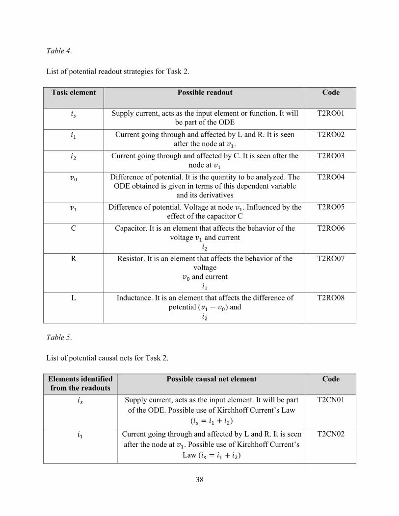
38
Table 4.
List of potential readout strategies for Task 2.
Task element Possible readout Code
Supply current, acts as the input element or function. It will be part of the ODE
T2RO01
Current going through and affected by L and R. It is seen after the node at .
T2RO02
Current going through and affected by C. It is seen after the node at
T2RO03
Difference of potential. It is the quantity to be analyzed. The ODE obtained is given in terms of this dependent variable
and its derivatives
T2RO04
Difference of potential. Voltage at node . Influenced by the effect of the capacitor C
T2RO05
C Capacitor. It is an element that affects the behavior of the voltage and current
T2RO06
R Resistor. It is an element that affects the behavior of the voltage
and current
T2RO07
L Inductance. It is an element that affects the difference of potential ( ) and
T2RO08
Table 5.
List of potential causal nets for Task 2.
Elements identified from the readouts
Possible causal net element Code
Supply current, acts as the input element. It will be part of the ODE. Possible use of Kirchhoff Current’s Law
( )
T2CN01
Current going through and affected by L and R. It is seen after the node at . Possible use of Kirchhoff Current’s
Law ( )
T2CN02

39
Also,
Current going through and affected by C. It is seen after the node at . Possible use of Kirchhoff Current’s Law
( )
1
T2CN03
Several inferences may come from this element. These are accounted for in the solution of the task from the
expert’s perspective.
T2CN04
Difference of potential. Voltage at node . Influenced by the effect of the capacitor C
1
T2CN05
C Capacitor. It is an element that affects the behavior of the voltage and current
1
T2CN06
R Resistor. It is an element that affects the behavior of the voltage
and current
T2CN07
L Inductance affecting the difference of potential and current
T2CN08
Finally, in the same way as I did with the other two tasks, I present Table 6. and Table 7 that
correspond to the possible readout strategies and causal nets for task 3. This task, in contrast with
the first two tasks, contained elements that did not need to be used as part of the set of readouts or
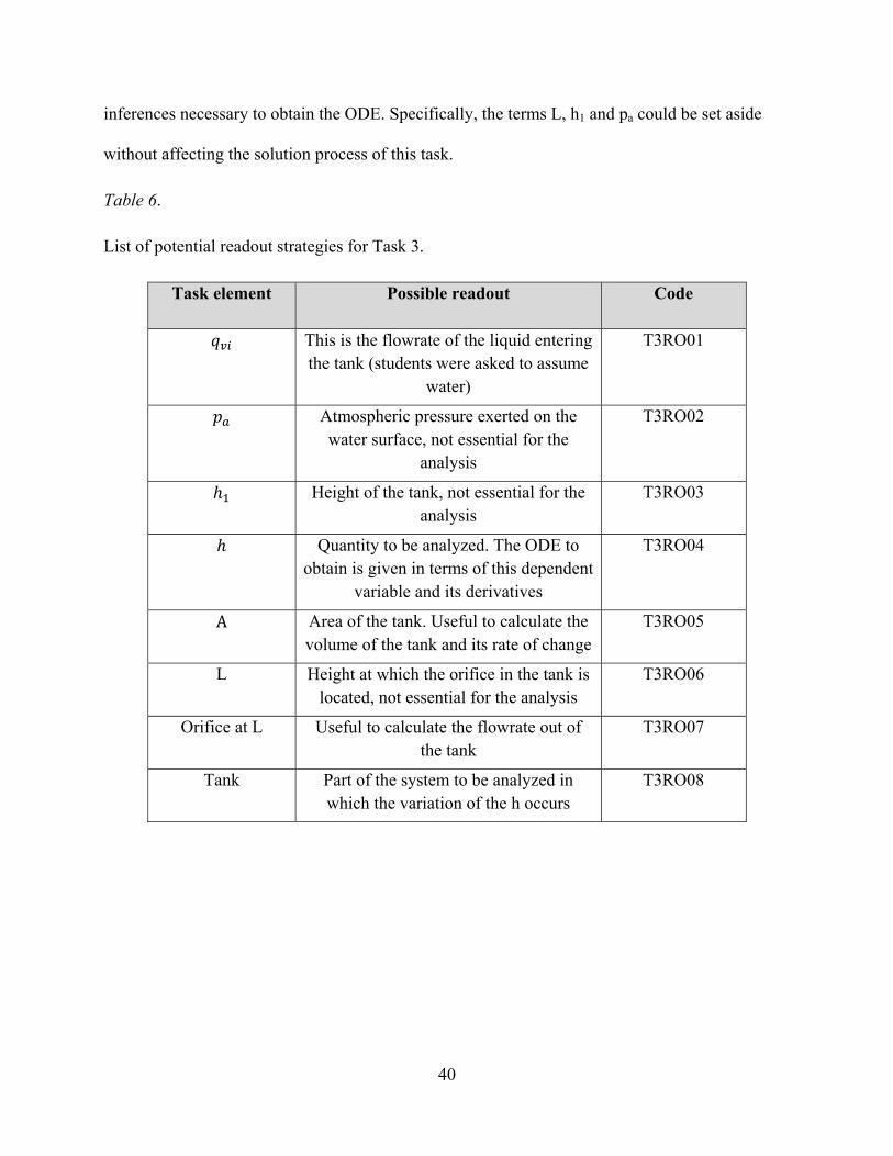
40
inferences necessary to obtain the ODE. Specifically, the terms L, h1 and pa could be set aside
without affecting the solution process of this task.
Table 6.
List of potential readout strategies for Task 3.
Task element Possible readout Code
This is the flowrate of the liquid entering the tank (students were asked to assume
water)
T3RO01
Atmospheric pressure exerted on the water surface, not essential for the
analysis
T3RO02
Height of the tank, not essential for the analysis
T3RO03
Quantity to be analyzed. The ODE to obtain is given in terms of this dependent
variable and its derivatives
T3RO04
A Area of the tank. Useful to calculate the volume of the tank and its rate of change
T3RO05
L Height at which the orifice in the tank is located, not essential for the analysis
T3RO06
Orifice at L Useful to calculate the flowrate out of the tank
T3RO07
Tank Part of the system to be analyzed in which the variation of the h occurs
T3RO08

41
Table 7.
List of potential causal nets for Task 3.
Elements identified from
the readouts
Possible causal net element Code
This flowrate is making the height of the tank increase. It is related to the Bernoulli’s equation
T3CN01
It is an indicator of the surrounding conditions of the problem. Not relevant for the purposes of the task
T3CN02
Height of the tank. This parameter is not relevant to the solution of the task
T3CN03
Quantity to be analyzed. The final ODE will be given in terms of this dependent variable and its derivatives. It seems
that the ODE will not contain second order terms
T3CN04
A Area of the tank. Useful to obtain the volume of the tank.
T3CN05
L This parameter is used only as a reference. From this
distance, water level changes, characterized as
T3CN06
Orifice at L This parameter is related to the flowrate coming out of the tank
2
T3CN07
Tank Element of the system where the variation of the quantity “h” occurs. It can be used as a control volume
T3CN08
Interviews
For the interviews, I scheduled two sessions with each student. In the first session I started
by talking about their responses to the survey and explained how the sessions would be
conducted. I informed them that the first session would take about 45 minutes in which they
would solve Task 1. I made sure that they had recently studied the topic of mechanical systems in

42
their system dynamics class in order to facilitate their thinking process. The sessions were video
recorded and students were asked to write and speak any idea that came to their minds as they
were solving the task. I also kept records of their work on the papers provided during the task.
About three weeks later I scheduled the second session. This time students were asked to
solve Tasks 2 and 3. Since this interview focused only the two tasks, each student took less than
40 minutes overall to solve or at least work on the two exercises the best they could. All sessions
were individual and the students relied on their knowledge only. That is, they did not count on
the help of any textbook, sheet of formulas or any other external help. This is a very important
aspect to mention since some of them alluded to this fact and how it would facilitate the work.
These aspects were taken into account as I present the results of the students’ work.
Data Analysis
The analysis of the students’ work consisted on analyzing two sources, the video
recordings of the interviews and students’ written work. The main analytic tool was the written
work, and the videos were used if clarification was needed for a student explanation or an
element of their written work.
I first reviewed each video in order to get an overall sense of how each student worked
with each task. This state enabled me to sketch their overall solution path. It was useful to begin
to perceive possible readouts and the causal nets for the students. After the first review of the
videos, most of the work was focused on the students’ written work. I performed the analysis in
three stages, where the first stage consisted of two simultaneous parts. I now proceed to describe
how each stage of the analysis was completed.

43
Stage One
The first stage consisted, first, of locating the readouts students used during the solution of
the task. I identified those elements that students considered as relevant to use in order to obtain
the ODE. The lists I provided of possible readout strategies in the previous section was helpful to
anticipate the kinds of things that might make up readouts for these students. Any readout
element that matched one in my list in the previous section was labelled as such. However, I also
recorded readouts that were not in my anticipated list. To identify a readout, any time a student
referred to a symbol or a part of the prompt and made an interpretation of it, I identified that as an
instance of a readout strategy. I recorded what the nature of that readout strategy was, in terms of
what they interpreted that symbol, part of the diagram, or wording of the task to mean. In the
same way, the second stage consisted of identifying the inferences made by the students using the
readouts with which they could eventually obtain an expression that represented an ODE model
of the system. Most of the work I did in these two parts of the first stage consisted on identifying
the readouts and causal nets, as the students worked on the tasks. I identified students’ readouts
when they considered a certain element as relevant for his/her analysis. For example, in task 1,
one of the elements was labelled as “k1”. This was the spring located at the top of the picture (see
Figure 4). The student could state that this element somehow influenced the system and was part
of the ODE, or that this spring produced a force acting on the pendulum or any similar statement;
this is an indication that the student “sees” this piece of information as relevant to set up the ODE
of the system. In this case, that is considered a readout. Most of the readouts were listed in the
tables shown earlier, so if a readout matched one in the table then it was labelled with the
assigned code for convenience.
44
On the other hand, a further step consisted of analyzing how the student used those
readouts. Continuing with the example of the spring 1 from task 1 (k1), a possible causal net
implied the recognition of this element yielding a moment2. In this case, the student infers that
the force of the spring produces a moment defined by the product of the force and the distance
from the center of rotation, for this task specifically it is defined as . Thus, if a student
showed evidence in his/her written work of this expression, then it was evidence of an activation
of the causal net for that corresponding readout, spring 1. Similarly as with the readouts, I listed
potential causal nets for the tasks and if the causal net matched one in the table, it was labelled
accordingly. As mentioned earlier, in addition to the list of potential readouts and causal net
elements, I left open the possibility of detecting others that were used by the students as they
worked on the tasks. These elements were recorded and were listed on a different table, as shown
in the results section.
Stage Two
In the theoretical background chapter I defined concept projections as the set of
knowledge and strategies used by an individual in a context in which a concept is applicable. In
this stage, I made use of the knowledge (readouts and causal nets) and attempted to infer the
strategies used by the students from the set of readouts and causal nets that helped them solve the
task. In other words, I operationalized these strategies so that I could find evidence of concept
projections. As I described concept projections in the theory chapter, I used the example of
quadratic equations to show the different representations in which these are presented. We
defined concept projection of roots in the factored context, or in the trinomial context. Each
concept projection involved a set of identifiable strategies and knowledge. In the same way, I
2 A moment is defined as the product of a force times a distance from the center in rotational systems

45
attempted to categorize the different strategies students used to approach the tasks. Sometimes
they used diagrams, or relied on the information from a specific equation or on the effects of the
components of the system in its behavior. I spotted at those sets of strategies and knowledge and
categorized them accordingly.
Stage Three
In this stage, I examined each strategy to determine whether it was productive for the
student in producing a solution to the task or not. This was done by observing (1) if the strategy
helped them achieve any kind solution at all, (2) whether the solution was correct, and (3)
whether the students had to revise their thinking or approach because of “dead ends.” In doing so,
I was able to observe which readouts and causal net elements allowed some students to progress
further than others. I was also able to observe difficulties students had during their solution
process, and could conjecture as to the possible readouts and causal net elements that factored
into the difficulty.
Pilot Study
Before carrying out this study, I interviewed Patrick, an undergraduate mechanical
engineering student. He volunteered for a pilot study in order to determine the possibility to use
the coordination class theory as presented in this document. Patrick was asked to solve a mass-
damper-spring system. Based on the theory, I identified the readouts and the causal nets although
I did not extend the analysis to hypothesize about concept projections. I briefly describe how I
identified the readouts and the causal nets in this pilot study.
In this task the student, Patrick, was asked to derive the equations of motion for the two
masses labelled as m1 and m2 as shown in Figure 8. In Figure 9, there are four parts that
comprised the analysis of readouts and causal nets. Section 1 indicates that this student was

46
attempting to make some inferences based on the information he saw as relevant (the readouts).
He was trying to remember different formulas learned in the past and that could have something
to do with the principle governing this system, Newton’s Second Law. The first two equations in
this section show that he recognized the effect of the spring in the system F=k(x), also, he
recognized the governing principle by writing the equation F=ma.
This last equation guided part of his reasoning in section 4 where he extended the
expression in an attempt to include all the elements of the system. Section 2 in Figure 9 evidences
Patrick’s recognition of the two masses as being relevant to obtain the equation of motion; that is,
these two drawings are readouts that, later on, are used to activate causal nets in sections 3 and 4
to obtain the ODE for one of the masses. Even though the expressions in sections 3 and 4 are not
entirely correct, still we might find evidence of Patrick’s attempts to use causal nets.
As I mentioned earlier, this pilot study helped me refine the process of identification of
readouts and causal nets. I could notice how a student recognized the relevant information and
not relying on the expert’s view only. Similarly, a student might come up with varied inferences
from what he/she “sees” from the task as well as the eventual selection of strategies; this pilot
study also served this purpose. I used this experience to analyze students’ work since it helped
me to be aware of the different ways in which students might interpret the tasks and the elements
in them. This pilot study also served as a reference to validate the possibility of applying the
concepts of the coordination class theory in this kind of contexts.

47
Figure 8. Mechanical system for the pilot study.
Figure 9. Analysis of a student’s work in a pilot study.
Further inferences from the readout
strategies

48
CHAPTER 5: RESULTS
In this results section, I start making an account of students’ answers to the survey’s
questions in order to highlight their mathematical knowledge regarding ODEs. Then, I describe
the tasks one at a time, starting with the first task for each student, then the second task and
finally the third task. I describe how the five different students attempted to work out a completed
differential equation and the processes they took to do that. Based on the stages described in the
data analysis section, I describe the readouts I identified, then the corresponding causal nets. I
also propose three overall solution strategies that emerged from the data by which the students
were able to progress toward setting up the ODE. These strategies, together with the readouts and
causal net elements that make them up, are considered to be concept projections of ODEs into
these contexts.
Finally, I discuss other aspects from the students’ written work, including decisions,
strategies and the use of other elements that hindered their processes to obtain the requested
ODE. Each student’s description will follow this pattern and though I make attempts to make the
account in the order described in this paragraph, in many passages I made mentions to all the
stages because of the decisions made by the students as they solved the tasks.
Analysis of Students’ Answers to the Survey
Table 8 shows the relevant pieces of information given by the students on the survey.
Some items were included from the initial conversation held in the first session of the interviews.
In that segment I attempted to complement the information they provided in the survey. For
question (1) related to what students understood for an ODE, the most common reference focused
on recognizing a second order equation because of the existence of a second derivative of y,
another common features were linearity and homogeneity although there were no explanations
49
related to these. Zane, Rebecca and Josh made mention of the fact that an ODE relates a variable
and its derivatives while Harry and Kira did not go further with their explanations, especially
Kira who had limited responses to all the questions in general.
With respect to questions (2) and (3) all of them related to the first and second derivatives,
and all but Kira related these to the contexts with which they are more familiar with, mechanical
systems, for this reason, they related these to velocity and acceleration. Question (4) related to the
dependent variable; in this question three of the students thought of it in terms of position,
matching what was mentioned about the previous questions (2) and (3) given the influence of the
mechanical systems.
In question (5) students related the constants with “coefficients” of the function and the
derivatives. Zane was the only one who indicated that these constants were related to the
parameters of the system, trying to provide a better interpretation of these elements. Three of
them, including Zane were more specific by relating these coefficients to the mass-spring-damper
system, thus moving away from the mathematical background and showing more influence from
the engineering and/or physical one. On the other hand, there was a general agreement as for
what they understood for question (6), which was related to the difference between the ODE
being equal to zero or any other value. There was consensus in indicating the when the ODE was
not equal to zero, there was an external function acting on the system and made it a forced
system. In this case there was no mention to any application or relation to an application from
physics or engineering except by Kira who briefly explained that it could be a “step” function, a
kind of function that is often used in the system dynamics course.
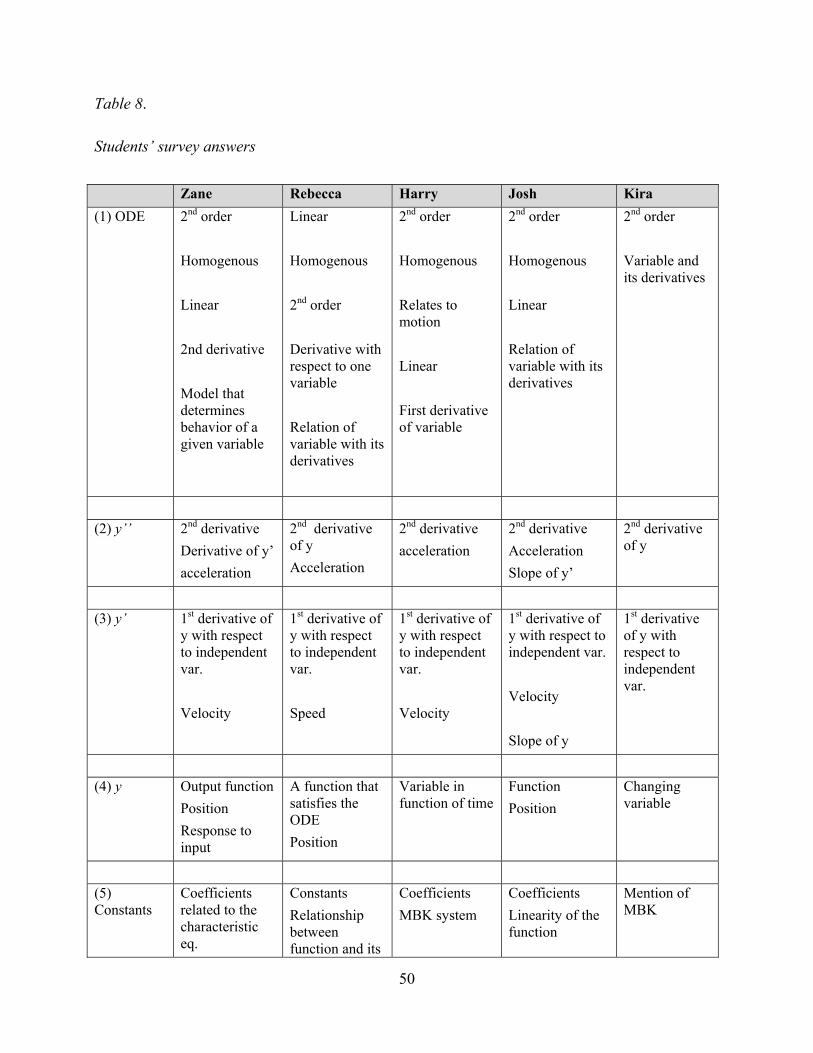
50
Table 8.
Students’ survey answers
Zane Rebecca Harry Josh Kira
(1) ODE 2nd order
Homogenous
Linear
2nd derivative
Model that determines behavior of a given variable
Linear
Homogenous
2nd order
Derivative with respect to one variable
Relation of variable with its derivatives
2nd order
Homogenous
Relates to motion
Linear
First derivative of variable
2nd order
Homogenous
Linear
Relation of variable with its derivatives
2nd order
Variable and its derivatives
(2) y’’ 2nd derivative
Derivative of y’
acceleration
2nd derivative of y
Acceleration
2nd derivative
acceleration
2nd derivative
Acceleration
Slope of y’
2nd derivative of y
(3) y’ 1st derivative of y with respect to independent var.
Velocity
1st derivative of y with respect to independent var.
Speed
1st derivative of y with respect to independent var.
Velocity
1st derivative of y with respect to independent var.
Velocity
Slope of y
1st derivative of y with respect to independent var.
(4) y Output function
Position
Response to input
A function that satisfies the ODE
Position
Variable in function of time
Function
Position
Changing variable
(5) Constants
Coefficients related to the characteristic eq.
Constants
Relationship between function and its
Coefficients
MBK system
Coefficients
Linearity of the function
Mention of MBK

51
System parameters
MBK system
derivatives
(6) Zero // Not zero
No forcing function or input
Non zero: Forced response + free response
External function applied to the system
Zero: Free response
Non zero: forced + free response
Input to the system
No other forces involved
“Heterogeneous”
Zero: No input
Non-zero: step or forced response
Analysis of Students’ Written Work for Task 1
Task 1 - Zane
At the beginning Zane recognized that the system in task 1 was governed by the principle
contained in the Newton’s Second Law understanding that the summation of the forces was equal
to the product of mass and acceleration, which in this case was the product of the moment of
inertia and the angular acceleration. Zane recognized that the pendulum was subject to the forces
exerted by the two springs and the damper and the ODE would contain this parameter, I.; in other
words: ∑ . This reasoning coincides with T1RO12, T1CN12 and T1CN13. From this
moment on, he attempted to explore the possibilities to obtain the mathematical model of the
system. Also, he considered relevant, and used in further steps, the direction of rotation of the
pendulum. Zane used it to determine the sign of each term of the final ODE.
Figure 10 shows the first excerpts made by Zane. In these, there is evidence of his ability
to recognize the pieces of information that he would require in order to set up the ODE. The
pieces circled in the figure show those elements considered the readouts of his work and coincide
with those predicted from the expert’s point of view.
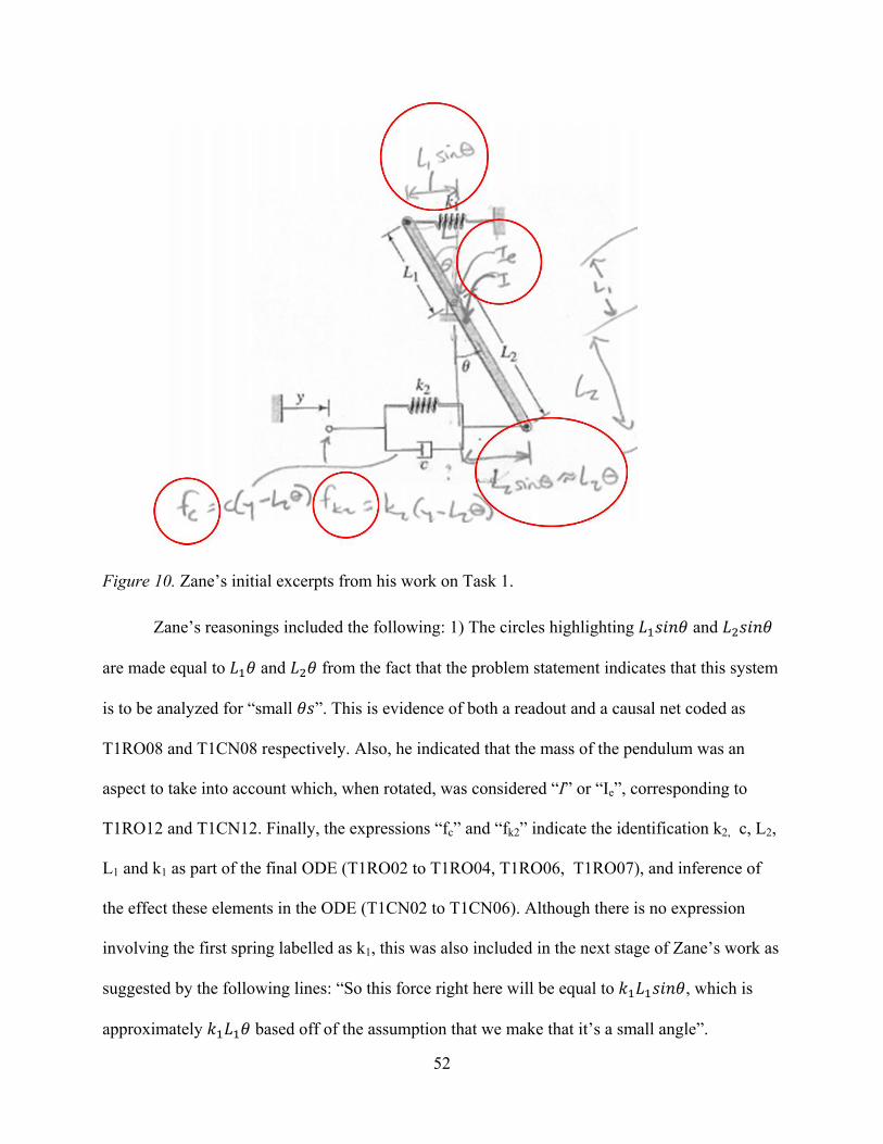
52
Figure 10. Zane’s initial excerpts from his work on Task 1.
Zane’s reasonings included the following: 1) The circles highlighting and
are made equal to and from the fact that the problem statement indicates that this system
is to be analyzed for “small ”. This is evidence of both a readout and a causal net coded as
T1RO08 and T1CN08 respectively. Also, he indicated that the mass of the pendulum was an
aspect to take into account which, when rotated, was considered “I” or “Ie”, corresponding to
T1RO12 and T1CN12. Finally, the expressions “fc” and “fk2” indicate the identification k2, c, L2,
L1 and k1 as part of the final ODE (T1RO02 to T1RO04, T1RO06, T1RO07), and inference of
the effect these elements in the ODE (T1CN02 to T1CN06). Although there is no expression
involving the first spring labelled as k1, this was also included in the next stage of Zane’s work as
suggested by the following lines: “So this force right here will be equal to , which is
approximately based off of the assumption that we make that it’s a small angle”.
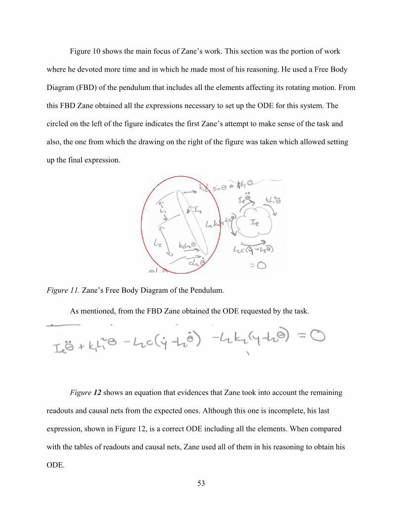
53
Figure 10 shows the main focus of Zane’s work. This section was the portion of work
where he devoted more time and in which he made most of his reasoning. He used a Free Body
Diagram (FBD) of the pendulum that includes all the elements affecting its rotating motion. From
this FBD Zane obtained all the expressions necessary to set up the ODE for this system. The
circled on the left of the figure indicates the first Zane’s attempt to make sense of the task and
also, the one from which the drawing on the right of the figure was taken which allowed setting
up the final expression.
Figure 11. Zane’s Free Body Diagram of the Pendulum.
As mentioned, from the FBD Zane obtained the ODE requested by the task.
Figure 12 shows an equation that evidences that Zane took into account the remaining
readouts and causal nets from the expected ones. Although this one is incomplete, his last
expression, shown in Figure 12, is a correct ODE including all the elements. When compared
with the tables of readouts and causal nets, Zane used all of them in his reasoning to obtain his
ODE.

54
Figure 12. Zane’s ODE.
When using all the readouts and making the inferences linked to those readouts, Zane
followed closely to what is described in the conceptual analysis of this task in the Methods
section. This does not mean that in order to finish the task successfully, students must use this
specific path. In contrast, there might be different ways to arrive to the same solution. In this
case, and taking into account the third stage of the analysis, the relevant aspect that allowed Zane
to use his readouts and facilitated the use of causal nets was his major use of the FBD. In this
way, when referring to the set of knowledge and strategies that enable the application of the
concept involved; that is, the relation between the quantity to be analyzed and its derivatives, the
projection of the concept was facilitated by the FBD. After I make an account of the Zane’s work
I refer to this aspect in more detail.
Figure 13. Zane’s final expression.
Finally, in this case, Zane did not seem to use strategies that hindered the process to
obtain the ODE. His work was straightforward and very close to that of the conceptual analysis
given in the methods section. The figure below shows an approximate flow of Zane’s reasoning

55
in this task. The labels in rectangular shape correspond to readouts (RO) and causal nets (CN)
correspondingly, the dashed arrows represent the approaches used by the students that activated
inferences or readouts. These approaches are described in more detail as they are presented in the
results of students’ work. In this section I introduce the approach used by Zane. Finally, the
dashed hexagon represents whether the student was successful, unsuccessful or partially
successful in obtaining the ODE for a given task.
Figure 14 shows the set of readouts, inferences and strategies used by Zane as he solved
task 1. He initially saw the relevance of the small angle (T1RO08) and the pendulum’s inertia
(T1RO12). Afterwards, the dashed line indicates the “Diagram approach” which, I argue, might
be the concept projection of the concept of the ODE for this specific context. This approach,
which will be explained in the next paragraph, helped Zane to activate the readouts and causal
nets (the set of boxes below the diagram arrow) that led him to obtain the ODE for this task
successfully. This figure is described in more detail below.
Diagram strategy. As shown in the description of Zane’s development of Task 1, he used
a Free Body Diagram as a tool to understand the behavior of the system as a whole but at the
same time, it enabled him to identify the effect that each component posed on the system. The
FDB (Diagram) facilitated his thinking process in these two ways.
In general, we might think of the diagram strategy as a general-to-specific approach that
helps the student focus on the overall system initially. Then, within that system, the student can
attend to individual elements without losing sight of the system as a whole. The diagram
approach resonates with certain methods used in engineering to describe a given system, such as
free-body diagrams, schematics or control volumes. Thus, as is seen in the following sections,
students could apply this approach to any of the three tasks.

56
As described in the theoretical framework, we can consider this to be a projection of the
concept of differential equation in the context of diagrams. This context enables the student to
use the readouts and causal nets to obtain the properties or characterize the quantity involved.
Summary of Zane’s flow of reasoning for Task 1. Each student’s task has been
described using figures similar to Figure 14. The rectangular shapes indicate either a readout
(RO) or a causal net (CN). Each readout and causal net was coded for each task (T1, T2 and T3);
also, each reaout and causal net has been numbered as indicated in tables 2 to 7. In this manner,
T1RO08 indicates the readout number 8 from Task 1 related to the identification of the small
angle theta in this task. It is also important to note that if the rectangle, or any other shape, has a
white font, then it means that it was properly activated and used in the task. On the other hand,
when a rectangle is gray, it means that that specific readout or causal net was not activated,
identified or improperly used; some of these readouts or causal nets were essential to complete
the task, others were not relevant.
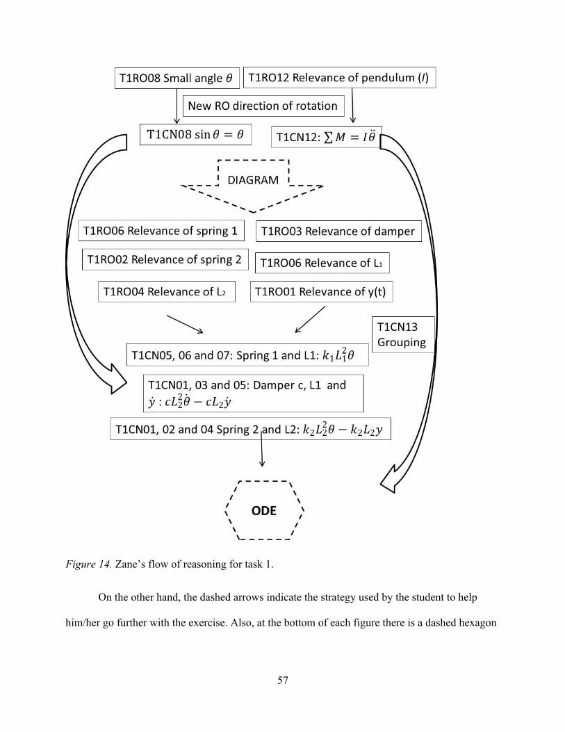
57
Figure 14. Zane’s flow of reasoning for task 1.
On the other hand, the dashed arrows indicate the strategy used by the student to help
him/her go further with the exercise. Also, at the bottom of each figure there is a dashed hexagon

58
that shows whether the student finished the task successfully, meaning that he/she found the right
ODE for the task or not.
In this case, Zane started by recognizing the importance of the small angle theta (T1RO08
and T1CN08) and the relevance of the pendulum (T1RO12 and T1CN12). Later on he used the
Diagram strategy which activated both the necessary readouts and causal nets that eventually led
him to obtain the ODE. The long and short arrows are used as an aid to indicate connection
between readouts and causal nets. Zane showed an adequate performance along all the process to
obtain the ODE. He came up with right causal nets and the strategy he chose (Diagram approach)
served his purposes well.
Task 1 – Rebecca
The first thoughts that Rebecca shared on this task were similar to those by Zane. She
identified the relevance of the small angle , T1RO08, and its implications, T1CN08. Next, she
wrote expressions in the picture indicating the recognition of the effect of the elements (k1, k2,
and c) as forces causing the pendulum to rotate corresponding to T1RO02, T1RO03 and
T1RO07.
In her following work, Rebecca started to think about the governing principle influencing
the system, the Newton’s Second Law. In this way, she recognized that the pendulum was
affected by the components, she recognized previously and from this reasoning she started to
develop the main part of her work to obtain the ODE, T1RO12. She struggled for a moment but
eventually came up with the following expression (T1CN12):

59
Figure 15. Rebecca’s identification of Newton’s Second Law for Task 1.
When asked about the meaning of the expression at the bottom in Figure 15, this is what
she replied:
Interviewer: What does that mean? That “I” and that “ ”?
Rebecca: The “I” is the inertia of the object and theta is the angular displacement, so means that it’s the second derivative with respect to time, meaning it’s the angular acceleration
The next thoughts implied the identification of the effect of each component on the
pendulum. Rebecca proceeded to focus on each of the components of the system in order to finish
the task. The expression below (Figure 16) indicates a partial solution of the task, she was able to
come up with it by relying on the effect of each component. Figure 16 evidences readout
strategies T1RO02, T1RO03 and T1RO07 that correspond to the recognition of the relevance of
the two springs and the damper, as well as the distances L1 and L2 correspondingly. This figure
also shows evidence of the use of causal nets that yield the moments produced by each
component. In this case, the terms indicate a partial expression that is completely reported in the
final answer.

60
Figure 16. Rebecca’s partial ODE.
After obtaining this partial equation, Rebecca went back to analyzing each of the
components in more detail. Figure 17 shows how she obtained analyzed each component
identifying readouts and making the corresponding inferences. Expressions Fk1, Fk2 and Fc were
obtained when the causal nets from the readouts , L1, L2, k1, k2, c, and were activated. In
terms of the codes assigned, she activated the following causal nets T1CN01 to 07 , and 09-10.
Figure 17. Rebecca’s component-based analysis of the system.
Rebecca’s analysis was carried out using a different approach than that used by Zane
(FBD, or Diagram approach); instead, she focused on the components of the system to eventually
put together all the pieces and set the equation. This approach is explained after Rebecca’s
account is completed. Rebecca was then able to finish this task successfully as shown in the
figure below:

61
Figure 18. Rebecca’s final ODE.
The analysis of Rebecca’s readouts and causal nets showed coincidence in most of the
ones predicted by the conceptual analysis presented in the methods section. In both cases, Zane
and Rebecca, there was no need to use T1RO11 and T1CN11 regarding the recognition of y = 0
and = 0 because these elements from the initial conditions are more useful when it comes to
solve the differential equation rather than at this stage when the student has to set up the
expression.
The analysis of Rebecca’s strategies used in conjunction with the set of readouts and
causal nets, evidenced a strong rely on the components effect on the system. In contrast with
Zane’s strategy, who used an FBD, Rebecca did not need to turn to this type of tool. The way that
she was able to arrive to a solution of the task focused mainly on the individual effect of the
elements and thus the projection was possible. This approach is explained in more detail in the
next paragraph after the description of Rebecca’s flow of reasoning in the task.
Summary of Rebecca’s flow of reasoning for Task 1. Figure 19 shows how
Rebecca approached this task. First, she identified the relevance of the small and the inertia of
the pendulum. Next, she used the component-based strategy to analyze each component of the
system (the effect of the springs and the damper along with the function y(t)). She worked on the
readouts and the corresponding causal nets activated by the concept projection from the
component-based approach that led her to obtain the ODE successfully.

62
Figure 19. Rebecca’s flow of reasoning for task 1.
Description of the Component strategy. This strategy consists on the identification and
focus on the components of a system that are ultimately part of the modeling expression. For
example, Rebecca’s solution of the task presented a detailed description of the effect of each of
the components of the system affecting the behavior of . She identified the effect of the two
springs as well as the damper in the system, and then determined how to put these elements
63
together into a coherent whole. There was no evidence of her using any diagram in order to
understand the system’s behavior and ultimately to obtain the ODE representing that behavior.
Thus, the difference between the component and diagram approaches is the guiding framework of
attention. Whereas the diagram approach places initial attention on the whole system, the
component approach places initial attention on individual pieces of the system and on how those
individual pieces relate to other information in the causal net that could be useful for producing
an ODE. In summary, the diagram approach is general-to-specific, while the component approach
is specific-to-general. It can also be considered as the concept projection of the differential
equation in the context of the components of the system.
This strategy was supported by an initial step in which Rebecca identified the governing
principle in the system (Newton’s Second Law). This action was an important activating strategy;
however, the main actions to obtain the final ODE, in the case of Rebecca, focused on the
component-based strategy.
Task 1 – Harry
Harry’s first thoughts on the task involved the fact that the pendulum had a mass even
though the task’s statement did not mention that:
Harry: the rod is not massless so… you need to draw a kind of reaction for the inertia of
the rod (pendulum) because, as you know, like, something the weights … is going to react
[inaudible] the pendulum is going to react to gravity or something”
Then, Harry wrote the term “mI” right next to the pendulum, and then the term “m ”.
This shows recognition of the role of the pendulum (T1RO12); however, the corresponding
causal net (T1CN12) was not activated. This was a first indication of a potential unsuccessful
setting up of the equation. See Figure 20.

64
Figure 20. Harry’s misinterpretation of the pendulum’s inertia.
After this initial analysis, Harry also indicated the importance of the small angle
(T1RO08) and used it afterwards in the expressions dealing with (T1CN08). His main
reasoning was focused on the components of the system, in this way he obtained a partial
expression, as shown in Figure 21, and led him to report his final ODE as seen on Figure 22.
Figure 21. Harry’s partial setting up of the ODE.
Nowhere in Figure 21 Harry shows evidence of inferring the effect of the forces from the
springs and the damper on the system, which at the same time should be observed in the
component analysis. Thus, even though he identified all the readouts for the successful
completion of this task, Harry did not make the right inferences that led to the proper
representation of the system’s ODE.
Figure 22. Harry’s final ODE.
On the other hand, despite the fact that Harry recognizes the relevance of the input y(t)
(T1RO09), he did not activate the causal nets necessary to imply this effect in the system
(T1CN09). Hence, Harry’s work was partially successful in the completion of this task.
65
Summary of Harry’s flow of reasoning for Task 1. Regarding the strategies he
activated for this task, Harry was mostly focused on a component-based analysis which was
insufficient to help him coordinate the inferences to indicate a proper effect of the components of
the system. His work on this task was limited to the excerpts shown in this account as well as
those in which he reasoned about the small angle and some minor notes on the effects of the
components. In this case, those notes did not lead him to express the moments caused by the
springs and damper properly. Figure 23 represents an approximation of his reasoning during this
task; those figures in grey shade represent inability to activate them. The one labelled with
T1CN12 implied that he could not completely infer the fact that there was a rotating system. On
the other hand, the rest of the gray rectangles are related to his difficulty to integrate the elements
of the ODE properly to obtain the right expression. Among these we find T1CN13 Grouping
which implied his inability to put all the elements together in the proper way to obtain a valid
ODE for this system.

66
Figure 23. Harry’s flow of reasoning for task 1.
Task 1 - Josh
In his initial reasoning, Josh did as the other students had done. Given that the statement
of the task indicated at its beginning that they were dealing with a small angle, this was the first
recognition and eventual inference of the task thus implying T1RO08 and T1CN08. On the other
hand, Josh drew a different version of the system, as shown in Figure 24. This diagram could be
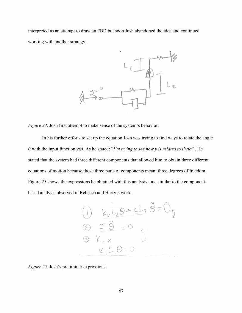
67
interpreted as an attempt to draw an FBD but soon Josh abandoned the idea and continued
working with another strategy.
Figure 24. Josh first attempt to make sense of the system’s behavior.
In his further efforts to set up the equation Josh was trying to find ways to relate the angle
with the input function y(t). As he stated: “I’m trying to see how y is related to theta” . He
stated that the system had three different components that allowed him to obtain three different
equations of motion because those three parts of components meant three degrees of freedom.
Figure 25 shows the expressions he obtained with this analysis, one similar to the component-
based analysis observed in Rebecca and Harry’s work.
Figure 25. Josh’s preliminar expressions.
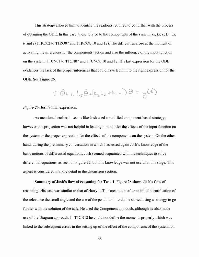
68
This strategy allowed him to identify the readouts required to go further with the process
of obtaining the ODE. In this case, those related to the components of the system: k1, k2, c, L1, L2,
and I (T1RO02 to T1RO07 and T1RO09, 10 and 12). The difficulties arose at the moment of
activating the inferences for the components’ action and also the influence of the input function
on the system: T1CN01 to T1CN07 and T1CN09, 10 and 12. His last expression for the ODE
evidences the lack of the proper inferences that could have led him to the right expression for the
ODE. See Figure 26.
Figure 26. Josh’s final expression.
As mentioned earlier, it seems like Josh used a modified component-based strategy;
however this projection was not helpful in leading him to infer the effects of the input function on
the system or the proper expression for the effects of the components on the system. On the other
hand, during the preliminary conversation in which I assessed again Josh’s knowledge of the
basic notions of differential equations, Josh seemed acquainted with the techniques to solve
differential equations, as seen on Figure 27, but this knowledge was not useful at this stage. This
aspect is considered in more detail in the discussion section.
Summary of Josh’s flow of reasoning for Task 1. Figure 28 shows Josh’s flow of
reasoning. His case was similar to that of Harry’s. This meant that after an initial identification of
the relevance the small angle and the use of the pendulum inertia, he started using a strategy to go
further with the solution of the task. He used the Component approach, although he also made
use of the Diagram approach. In T1CN12 he could not define the moments properly which was
linked to the subsequent errors in the setting up of the effect of the components of the system; on
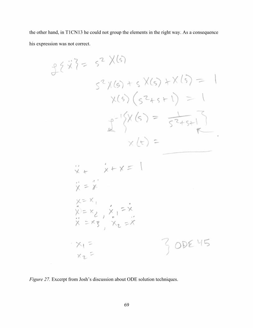
69
the other hand, in T1CN13 he could not group the elements in the right way. As a consequence
his expression was not correct.
Figure 27. Excerpt from Josh’s discussion about ODE solution techniques.
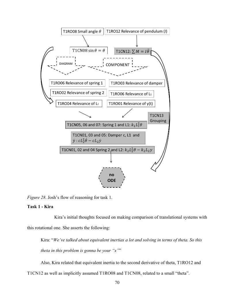
70
Figure 28. Josh’s flow of reasoning for task 1.
Task 1 - Kira
Kira’s initial thoughts focused on making comparison of translational systems with
this rotational one. She asserts the following:
Kira: “We’ve talked about equivalent inertias a lot and solving in terms of theta. So this
theta in this problem is gonna be your “x””
Also, Kira related that equivalent inertia to the second derivative of theta, T1RO12 and
T1CN12 as well as implicitly assumed T1RO08 and T1CN08, related to a small “theta”.
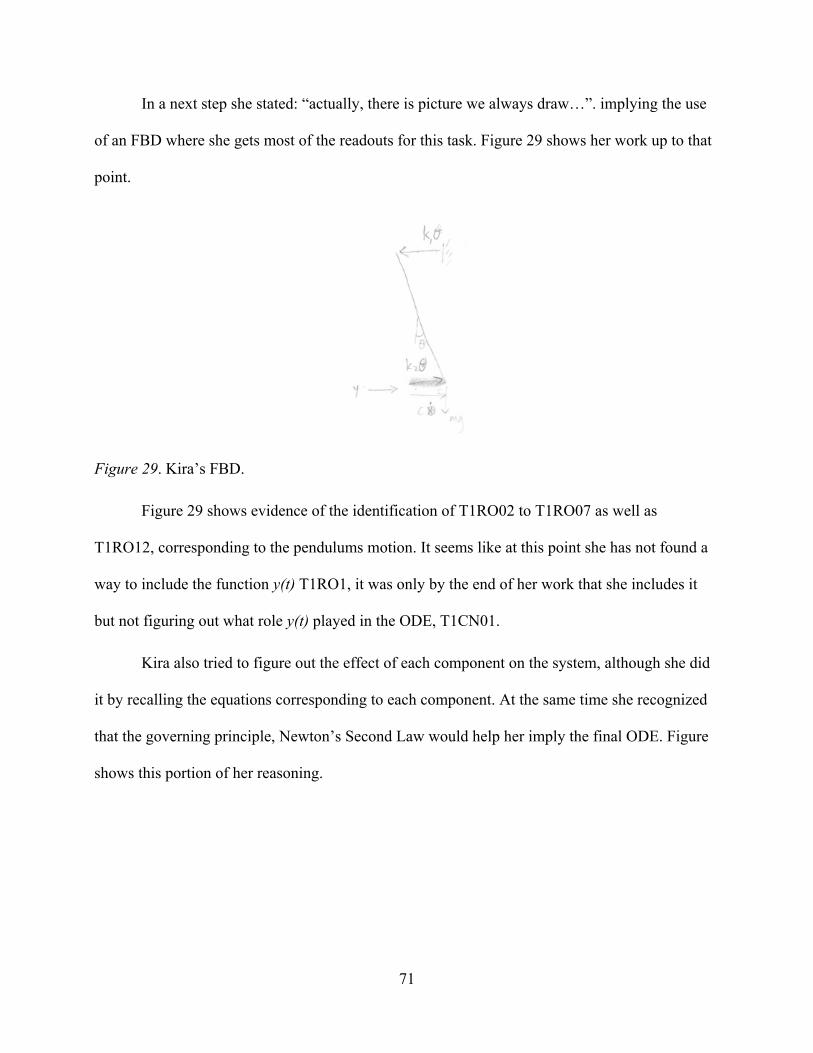
71
In a next step she stated: “actually, there is picture we always draw…”. implying the use
of an FBD where she gets most of the readouts for this task. Figure 29 shows her work up to that
point.
Figure 29. Kira’s FBD.
Figure 29 shows evidence of the identification of T1RO02 to T1RO07 as well as
T1RO12, corresponding to the pendulums motion. It seems like at this point she has not found a
way to include the function y(t) T1RO1, it was only by the end of her work that she includes it
but not figuring out what role y(t) played in the ODE, T1CN01.
Kira also tried to figure out the effect of each component on the system, although she did
it by recalling the equations corresponding to each component. At the same time she recognized
that the governing principle, Newton’s Second Law would help her imply the final ODE. Figure
shows this portion of her reasoning.
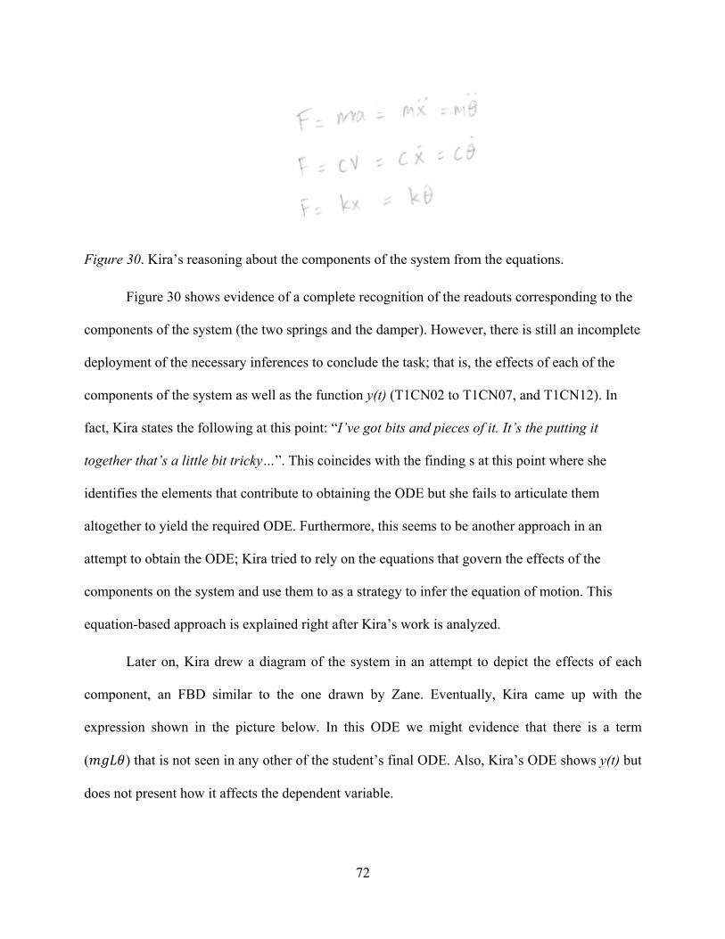
72
Figure 30. Kira’s reasoning about the components of the system from the equations.
Figure 30 shows evidence of a complete recognition of the readouts corresponding to the
components of the system (the two springs and the damper). However, there is still an incomplete
deployment of the necessary inferences to conclude the task; that is, the effects of each of the
components of the system as well as the function y(t) (T1CN02 to T1CN07, and T1CN12). In
fact, Kira states the following at this point: “I’ve got bits and pieces of it. It’s the putting it
together that’s a little bit tricky…”. This coincides with the finding s at this point where she
identifies the elements that contribute to obtaining the ODE but she fails to articulate them
altogether to yield the required ODE. Furthermore, this seems to be another approach in an
attempt to obtain the ODE; Kira tried to rely on the equations that govern the effects of the
components on the system and use them to as a strategy to infer the equation of motion. This
equation-based approach is explained right after Kira’s work is analyzed.
Later on, Kira drew a diagram of the system in an attempt to depict the effects of each
component, an FBD similar to the one drawn by Zane. Eventually, Kira came up with the
expression shown in the picture below. In this ODE we might evidence that there is a term
( ) that is not seen in any other of the student’s final ODE. Also, Kira’s ODE shows y(t) but
does not present how it affects the dependent variable.

73
Figure 31. Kira’s final ODE.
Figure 32. Kira’s flow of reasoning for task 1.
Summary of Kira’s flow of reasoning for Task 1. Kira identified, just like the other
students, the relevance of the angle and the role of the pendulum’s inertia. She used the Diagram
strategy to help her notice the relevance and role of the elements of the system. She then
74
proceeded to use Equation and Component strategy to make an attempt to put together all the
elements (T1CN13) of the ODE. However, similar to Josh and Harry, Kira got stuck on the
impossibility to understand the role of the input function (T1CN01) and could not provide an
accurate expression at the end even though she had noticed its relevance (T1RO01).
Equation strategy. This strategy seems to rely on the fact that there is a main equation
representing the governing principle acting on the system. From that equation the student centers
all his/her efforts to obtain the ODE by manipulating the equation or making substitutions into
the equation. For example, as we see in the electrical context, the student might start his work
recognizing the KCL and base all his/her reasoning on the equation is=i1+i2 . A student using this
approach begins with this equation and attempts to identify how each part of the equation fits
with the context in order to transform the base equation, through substitutions and other
manipulations, into an ODE. In this case, we might consider this, the concept projection of the
differential equation in the context of the equation.
In general, students used this strategy as an ancillary tool when solving Task 1. In the
next two tasks we might notice that this strategy played a stronger role beyond that of only
identifying the governing principle of the system.
Summary of the Strategies
So far I identified three sets of strategies used by the students in order to assist them to solve the
tasks: (1) Diagram strategy, (2) Component strategy and (3) Equation strategy. The diagram-
based strategy involves the use of any diagram or depiction of the system in a simpler
representation. This approach includes the identification of any element in the system that affects

75
the system behavior. In the following analysis of the tasks I describe other examples of Diagrams
depending on the context; Free Body Diagrams are one of these examples.
The second strategy, the Component-based strategy, entails focusing on each of the system’s
components; infer its effects on the system and then figure out the integration of those
components in the whole. As discussed earlier, the diagram approach is general-to-specific, while
the component approach is specific-to-general.
The equation-based approach relies on an equation that governs the system’s behavior and, by
making substitutions and manipulations, converts the equation into an ODE. This approach was
very useful for students when solving task 3, the fluid system, as we may see in the
corresponding analysis.
Analysis of Students’ Written Work for Task 2
Task 2 – Zane
As task 2 was presented, Zane initially departed from the stated objective of producing an
ODE that models the situation, and instead thought of the Laplace transform method. The
Laplace method takes the domain and changes to be “s”, a complex variable, instead of time (t).
The Laplace method is meant to facilitate the solution of this type of exercises, but at the same
time, it avoids the issue of creating an ODE altogether. Thus, using the Laplace method steered
Zane away from the initial goal of the task. Its complexities became a problem not only for him
but for other students who decided to use this strategy to solve the task. On the other hand, the
exercise taken from a textbook (Palm, 2005), was designed in such a way that students do not
need to turn to the Laplace strategy to obtain the ODE.
After attempting the Laplace transform method, Zane then returned to the task of
producing an ODE by writing an outline of the potential effects of the components of the circuit

76
in the system. In Figure 33 it can be seen that Zane recognized the relevance of all the elements
of the system; that is: the currents (is, i1, i2), the components: the capacitor (C), the resistance (R)
and the inductance (L); and the voltages (v1 and vo) (T2RO01 to T1RO08). With respect to the
causal nets for this task, Zane could only activate those corresponding to the currents is, i1 and i2
(T2CN01 to 03) as evidenced in the same picture.
Before finishing all his work for this task, Zane referred to the three expressions at the
bottom of Figure 33:
“so we could combine these relationships just the same way I am doing here
[pointing at Laplace equation] in terms of Kirchhoff’s Current Law. It’s just that, since
they’re time derivatives in voltage and current it’s a little bit harder to manipulate and
integrate things”.
What Zane expresses at this point indicates his lack of knowledge to finish his task
successfully. He was not able to articulate strategies to allow him to coordinate the elements of
which he already had information from. This is a situation in which it is possible to argue that he
lacks the possibility to operate a concept projection. His first attempt entailed the tools provided
by the Laplace method, eventually he tried to use the component-based strategy but he was not
able to articulate the causal nets T1CN04 to T1CN08.
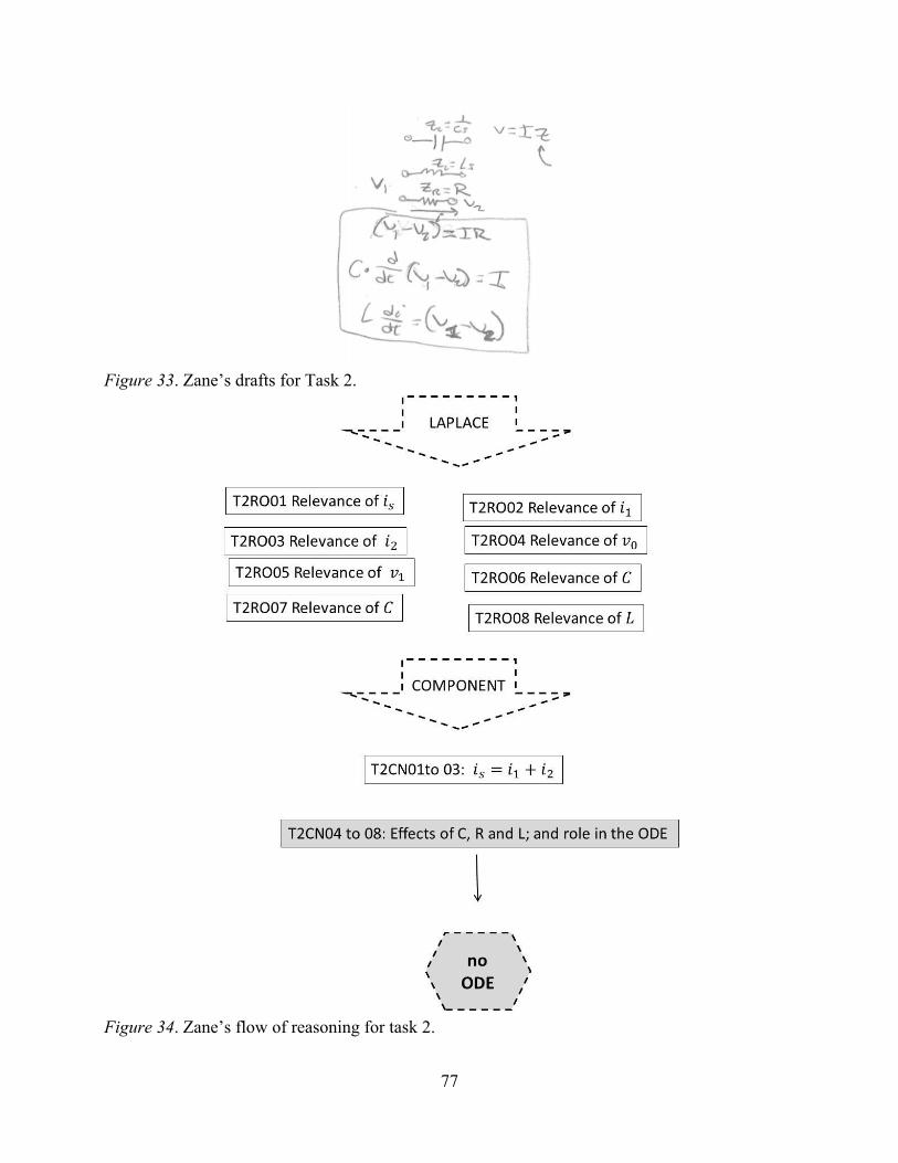
77
Figure 33. Zane’s drafts for Task 2.
Figure 34. Zane’s flow of reasoning for task 2.

78
Summary of Zane’s flow of reasoning for Task 2. Zane started this task by trying to use
the Laplace method but given that he did not have any aid, like a textbook or a sheet of formulas
to help him go further, he discarded this option. During that process though, he noticed the
relevance of the elements of the system and thus he proceeded to use the Component strategy that
allowed him to infer that the system was governed by the Kirchhoff’s Current Law, writing the
equation shown in T2CN01 to 03 in the figure. However, he had problems to infer the specific
role of the elements (T2CN04 to 08) not obtaining the desired ODE this time.
Task 2 – Rebecca
Obtaining the model of the voltage was a particular challenge for the participating
students. Rebecca was probably the student whose final ODE showed the closest resemblance to
the actual solution of the task. Rebecca initially recognized that the circuit was ruled by the
Kirchhoff Current Law. From this law the individual may focus on the nodes of the circuit and
infer that the current entering the node equals the current leaving the node. This indicates T2RO1
to 03 and T2CN01 to 03 correspondingly. See figure below.
Figure 35. Rebecca’s initial work on Task 2.

79
Figure 36. Rebecca’s diagram of the circuit.
After writing this initial equation, Rebecca changed the strategy and started to focus on
the components of the circuit. She did this in an attempt to integrate the results of both strategies
to be able to obtain a new expression for . She showed some understanding of the effect that
each component exerted on the system; nevertheless, as it was not enough for her to go further,
she tried drawing a sketch of the circuit as shown in Figure 36.
This rearrangement of the circuit allowed Rebecca to see a different perspective of the
system as a whole and, at the same time, focus on the effect of the components, just as described
previously, relevance of all the elements in the system: currents, voltages, capacitor, inductance
and resistance (T1RO01 to T1RO08) as well as the equation taken from KCL: T1CN01 to 03. In
fact, she tried to articulate what she had found as she used each strategy but her efforts were
fruitless beyond that point. The figure below shows her last final answer for Task 2.
Figure 37. Rebecca’s final expression.

80
In Rebecca’s case, we might notice her intention to obtain an expression where is the
dependent variable, as well as relating it with its derivatives; however, she lacked the elements
(knowledge) to coordinate her ideas in a way that she could get to the right answer.
Summary of Rebecca’s flow of reasoning for Task 2. Rebecca decided to start working
on the Task using the Diagram strategy and then, almost immediately, the Component strategy.
At doing this she activated the readouts for all the elements of the system. When these relevant
elements were identified, she then proceeded to use the Equation strategy in an attempt to obtain
the ODE. From the equation she could infer some of the effects of the elements but in an
incomplete way (T2CN04 to 08); in this manner, although she was the one who got closer to a
proper ODE for the system, she could not obtain that final expression. Specifically, for all the
students, the role of the inductance (T2CN08) played a significant role to obtain the final
expression but none of them could accurately infer it form the Task.
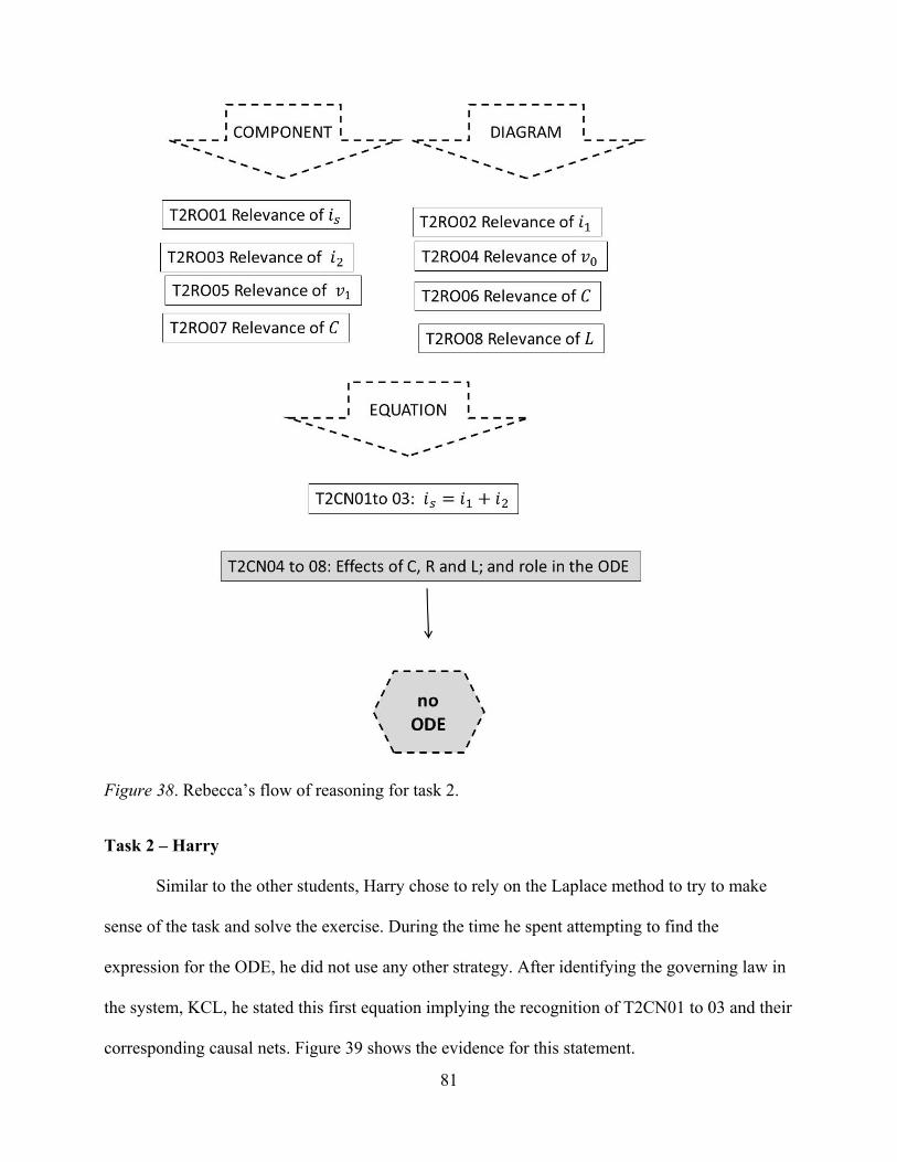
81
Figure 38. Rebecca’s flow of reasoning for task 2.
Task 2 – Harry
Similar to the other students, Harry chose to rely on the Laplace method to try to make
sense of the task and solve the exercise. During the time he spent attempting to find the
expression for the ODE, he did not use any other strategy. After identifying the governing law in
the system, KCL, he stated this first equation implying the recognition of T2CN01 to 03 and their
corresponding causal nets. Figure 39 shows the evidence for this statement.

82
Figure 39. Harry’s evidence of KCL use.
As mentioned earlier, Harry did not rely on any other strategy except by Laplace method
so he tried to make several inferences that came up to be useless to obtain a valid expression. In
fact, not much can be said about Harry’s work up to this point given that his excerpts did not
evidence usable elements to imply the proper use of the causal nets expected for this task
(T2CN01 to T1CN08). Furthermore, his last expression lacked the basic elements expected from
an ODE for this case; that is, there is no dependent variable or its derivatives as shown in Figure
40.
Figure 40. Harry’s final expression (ODE).
Summary of Harry’s flow of reasoning for Task 2. Harry attempted to use the Equation
strategy from which he identified some elements of relevance. However, although he had
identified the governing principle, he did not go much further so he decided to turn to the Laplace
method in an effort to obtain the final expression. At this moment, it seems like he lost track of
the process; he could not infer what the role of each element was, and consequently failed to
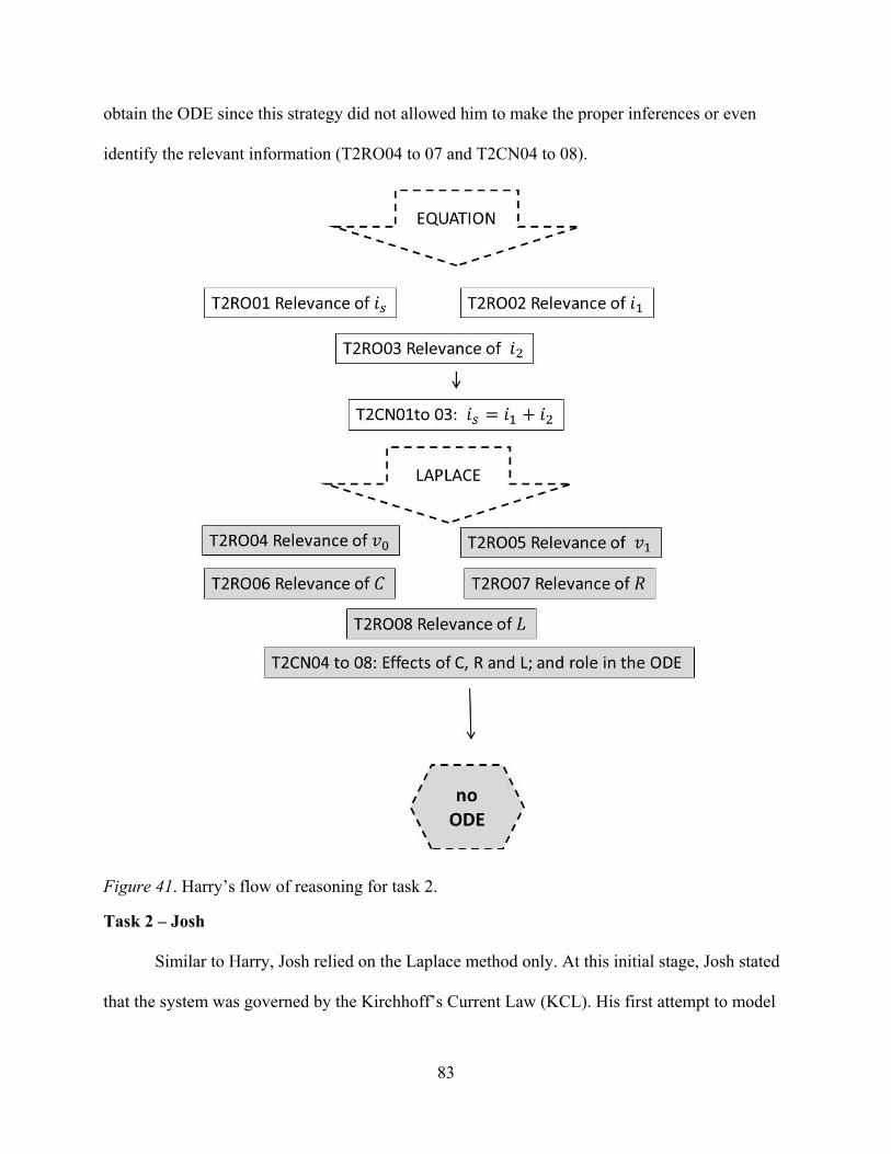
83
obtain the ODE since this strategy did not allowed him to make the proper inferences or even
identify the relevant information (T2RO04 to 07 and T2CN04 to 08).
Figure 41. Harry’s flow of reasoning for task 2.
Task 2 – Josh
Similar to Harry, Josh relied on the Laplace method only. At this initial stage, Josh stated
that the system was governed by the Kirchhoff’s Current Law (KCL). His first attempt to model
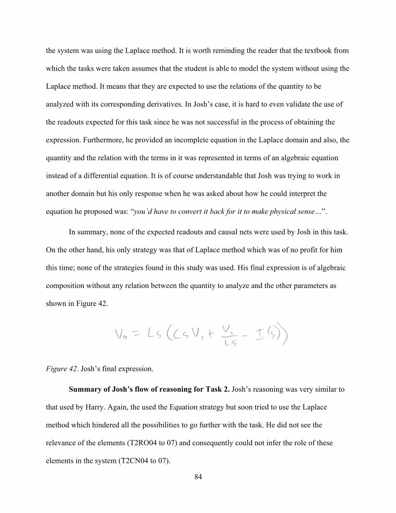
84
the system was using the Laplace method. It is worth reminding the reader that the textbook from
which the tasks were taken assumes that the student is able to model the system without using the
Laplace method. It means that they are expected to use the relations of the quantity to be
analyzed with its corresponding derivatives. In Josh’s case, it is hard to even validate the use of
the readouts expected for this task since he was not successful in the process of obtaining the
expression. Furthermore, he provided an incomplete equation in the Laplace domain and also, the
quantity and the relation with the terms in it was represented in terms of an algebraic equation
instead of a differential equation. It is of course understandable that Josh was trying to work in
another domain but his only response when he was asked about how he could interpret the
equation he proposed was: “you’d have to convert it back for it to make physical sense…”.
In summary, none of the expected readouts and causal nets were used by Josh in this task.
On the other hand, his only strategy was that of Laplace method which was of no profit for him
this time; none of the strategies found in this study was used. His final expression is of algebraic
composition without any relation between the quantity to analyze and the other parameters as
shown in Figure 42.
Figure 42. Josh’s final expression.
Summary of Josh’s flow of reasoning for Task 2. Josh’s reasoning was very similar to
that used by Harry. Again, the used the Equation strategy but soon tried to use the Laplace
method which hindered all the possibilities to go further with the task. He did not see the
relevance of the elements (T2RO04 to 07) and consequently could not infer the role of these
elements in the system (T2CN04 to 07).

85
Figure 43. Josh’s flow of reasoning for task 2.
Task 2 – Kira
Kira’s work on this task involved the use of two strategies. In her first attempt she tried to
analyze the effect of each element of the circuit using the component-based approach (Figure 44).
In this case, Kira identified the relevance of each element of the system, matching those
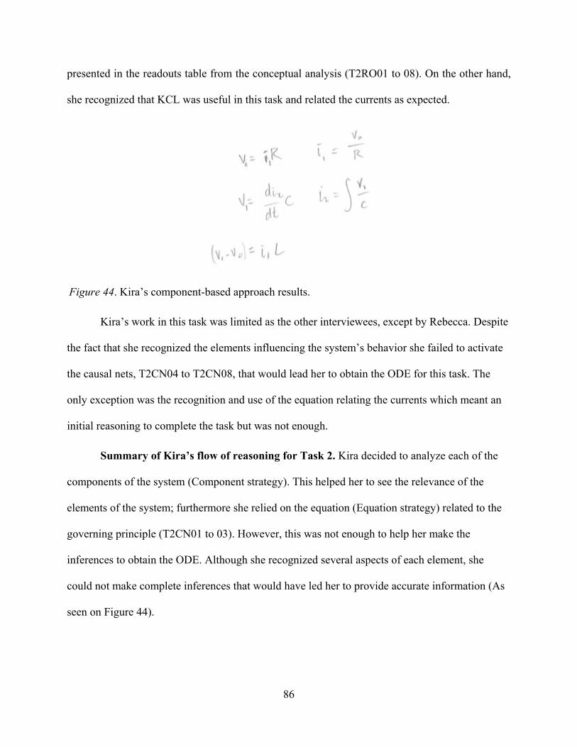
86
presented in the readouts table from the conceptual analysis (T2RO01 to 08). On the other hand,
she recognized that KCL was useful in this task and related the currents as expected.
Figure 44. Kira’s component-based approach results.
Kira’s work in this task was limited as the other interviewees, except by Rebecca. Despite
the fact that she recognized the elements influencing the system’s behavior she failed to activate
the causal nets, T2CN04 to T2CN08, that would lead her to obtain the ODE for this task. The
only exception was the recognition and use of the equation relating the currents which meant an
initial reasoning to complete the task but was not enough.
Summary of Kira’s flow of reasoning for Task 2. Kira decided to analyze each of the
components of the system (Component strategy). This helped her to see the relevance of the
elements of the system; furthermore she relied on the equation (Equation strategy) related to the
governing principle (T2CN01 to 03). However, this was not enough to help her make the
inferences to obtain the ODE. Although she recognized several aspects of each element, she
could not make complete inferences that would have led her to provide accurate information (As
seen on Figure 44).

87
Figure 45. Kira’s flow of reasoning for task 2.
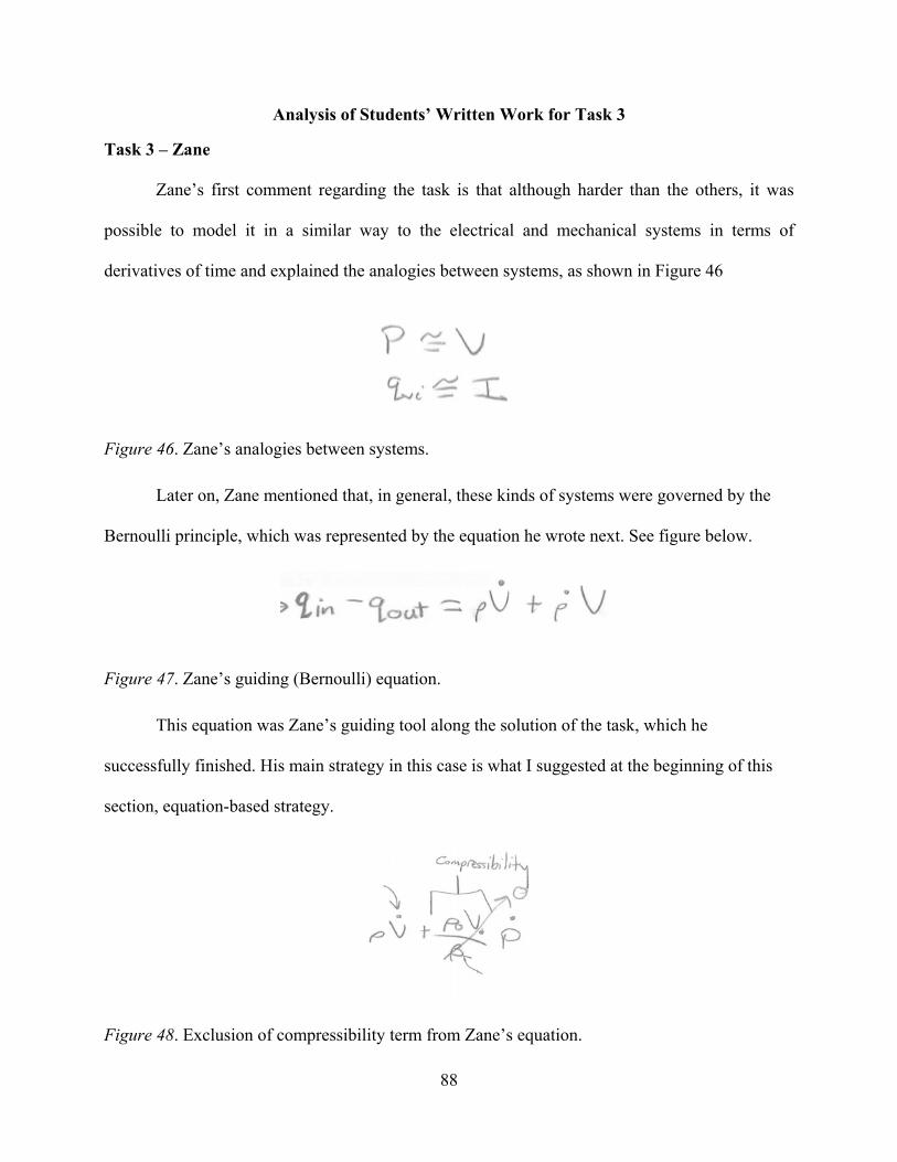
88
Analysis of Students’ Written Work for Task 3
Task 3 – Zane
Zane’s first comment regarding the task is that although harder than the others, it was
possible to model it in a similar way to the electrical and mechanical systems in terms of
derivatives of time and explained the analogies between systems, as shown in Figure 46
Figure 46. Zane’s analogies between systems.
Later on, Zane mentioned that, in general, these kinds of systems were governed by the
Bernoulli principle, which was represented by the equation he wrote next. See figure below.
Figure 47. Zane’s guiding (Bernoulli) equation.
This equation was Zane’s guiding tool along the solution of the task, which he
successfully finished. His main strategy in this case is what I suggested at the beginning of this
section, equation-based strategy.
Figure 48. Exclusion of compressibility term from Zane’s equation.
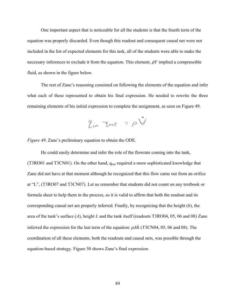
89
One important aspect that is noticeable for all the students is that the fourth term of the
equation was properly discarded. Even though this readout and consequent causal net were not
included in the list of expected elements for this task, all of the students were able to make the
necessary inferences to exclude it from the equation. This element, implied a compressible
fluid, as shown in the figure below.
The rest of Zane’s reasoning consisted on following the elements of the equation and infer
what each of these represented to obtain his final expression. He needed to rewrite the three
remaining elements of his initial expression to complete the assignment, as seen on Figure 49.
Figure 49. Zane’s preliminary equation to obtain the ODE.
He could easily determine and infer the role of the flowrate coming into the tank,
(T3RO01 and T3CN01). On the other hand, qout required a more sophisticated knowledge that
Zane did not have at that moment although he recognized that this flow came out from an orifice
at “L”, (T3RO07 and T3CN07). Let us remember that students did not count on any textbook or
formula sheet to help them in the process, so it is valid to affirm that both the readout and its
corresponding causal net are properly inferred. Finally, by recognizing that the height (h), the
area of the tank’s surface (A), height L and the tank itself (readouts T3RO04, 05, 06 and 08) Zane
inferred the expression for the last term of the equation: (T3CN04, 05, 06 and 08). The
coordination of all these elements, both the readouts and causal nets, was possible through the
equation-based strategy. Figure 50 shows Zane’s final expression.
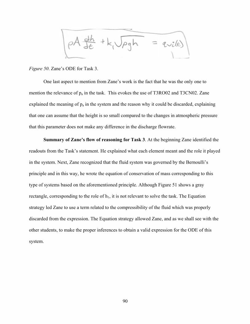
90
Figure 50. Zane’s ODE for Task 3.
One last aspect to mention from Zane’s work is the fact that he was the only one to
mention the relevance of pa in the task. This evokes the use of T3RO02 and T3CN02. Zane
explained the meaning of pa in the system and the reason why it could be discarded, explaining
that one can assume that the height is so small compared to the changes in atmospheric pressure
that this parameter does not make any difference in the discharge flowrate.
Summary of Zane’s flow of reasoning for Task 3. At the beginning Zane identified the
readouts from the Task’s statement. He explained what each element meant and the role it played
in the system. Next, Zane recognized that the fluid system was governed by the Bernoulli’s
principle and in this way, he wrote the equation of conservation of mass corresponding to this
type of systems based on the aforementioned principle. Although Figure 51 shows a gray
rectangle, corresponding to the role of h1, it is not relevant to solve the task. The Equation
strategy led Zane to use a term related to the compressibility of the fluid which was properly
discarded from the expression. The Equation strategy allowed Zane, and as we shall see with the
other students, to make the proper inferences to obtain a valid expression for the ODE of this
system.
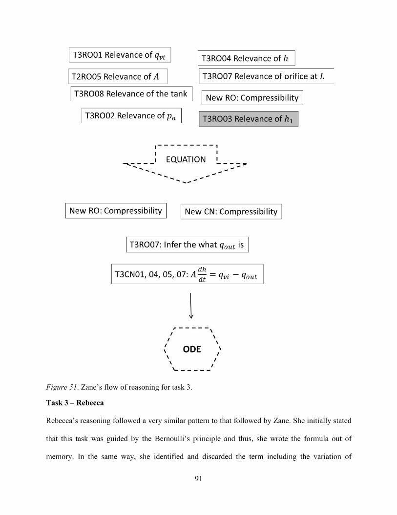
91
Figure 51. Zane’s flow of reasoning for task 3.
Task 3 – Rebecca
Rebecca’s reasoning followed a very similar pattern to that followed by Zane. She initially stated
that this task was guided by the Bernoulli’s principle and thus, she wrote the formula out of
memory. In the same way, she identified and discarded the term including the variation of
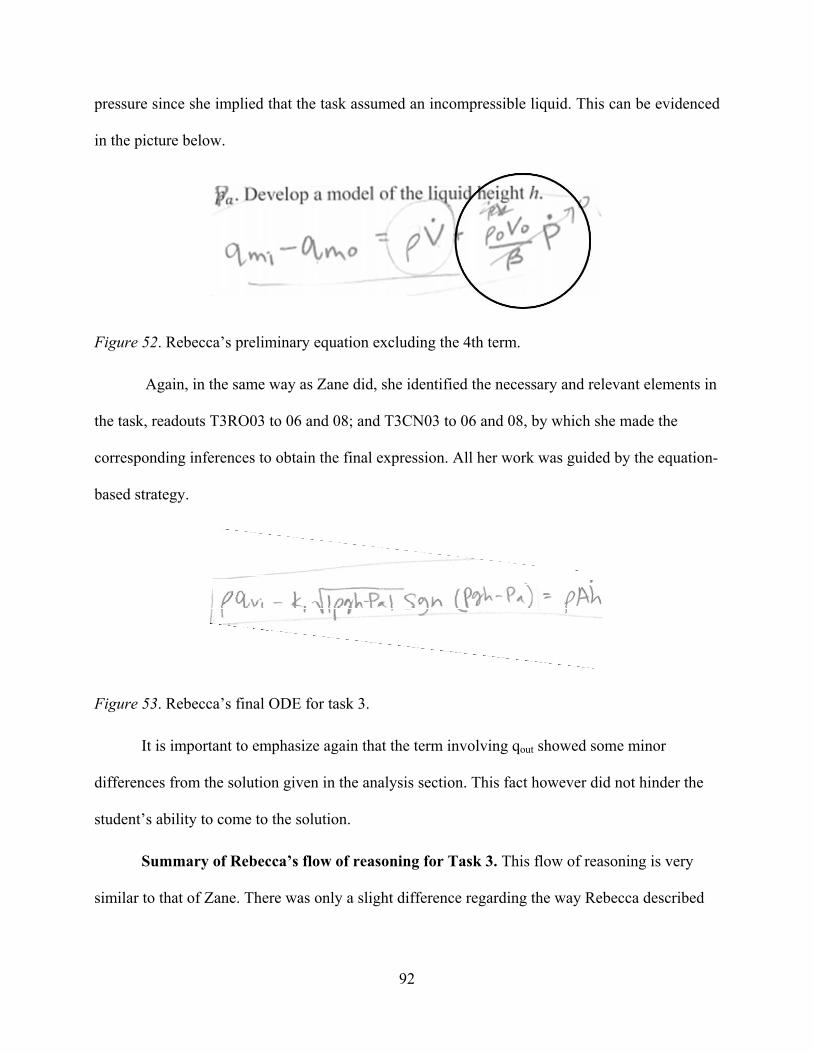
92
pressure since she implied that the task assumed an incompressible liquid. This can be evidenced
in the picture below.
Figure 52. Rebecca’s preliminary equation excluding the 4th term.
Again, in the same way as Zane did, she identified the necessary and relevant elements in
the task, readouts T3RO03 to 06 and 08; and T3CN03 to 06 and 08, by which she made the
corresponding inferences to obtain the final expression. All her work was guided by the equation-
based strategy.
Figure 53. Rebecca’s final ODE for task 3.
It is important to emphasize again that the term involving qout showed some minor
differences from the solution given in the analysis section. This fact however did not hinder the
student’s ability to come to the solution.
Summary of Rebecca’s flow of reasoning for Task 3. This flow of reasoning is very
similar to that of Zane. There was only a slight difference regarding the way Rebecca described

93
the expression for qout ; in both cases, should the students have the usual aids they had obtained
the exact expression. Other than that, the Equation strategy served very well to Rebecca.
Figure 54. Rebecca’s flow of reasoning for task 3.

94
Task 3 – Harry
In order to avoid repetition in the account, it is sufficient to mention that Harry attempted
to follow the same reasoning evidenced by Rebecca and Zane. However, I focus on two
important aspects of his work.
The first differentiating feature in Harry’s work deals with the fact that he used more than
one strategy (Equation-based) to solve the task. As part of his initial analysis, Harry used the tank
as a control volume. A control volume is a closed region used in thermofluids to determine what
elements produce a change in its volume/mass. In this way, this approach coincides with the FBD
strategy used in the mechanical task, thus it can be considered a diagram-based strategy to help
project the concept to analyze. Due to the use of the control volume Harry used T3RO08 and
T3CN08 to help him make sense of the variation of volume in the tank.
There was a second factor in Harry’s work that differed from Zane and Rebecca’s. He did
not discard the compressibility term from his final answer. Even though he was informed that the
task assumed water (an incompressible fluid), he replied:
Interviewer: Let’s assume it’s water…
Harry: OK, so assuming it’s water, I don’t know what that would be again, I will just take that “beta” all the way to my final answer...”
In this way, Harry decided to keep this term and the figure below, Figure 55, shows his
final answer. He identified and operated all the readouts and causal nets expected for this task
except by T3RO02 and T3CN02, which anyway, are not fundamental to come to the final
answer. However, this additional readout, the recognition of the compressibility factor in the
equation, was not properly inferred, in other words, the causal net was not properly applied so he
could have obtained the right final answer.

95
Figure 55. Harry’s final ODE for task 3.
Figure 56. Harry’s flow of reasoning for task 3.
Summary of Harry’s flow of reasoning for Task 3. The only difference between
Harry’s flow of reasoning and the previous students implied that besides using the Equation

96
strategy, he also used the Diagram strategy. This strategy helped Harry see how the water level
(h) changed; he could also identify the corresponding relevant elements and inferences to obtain
the ODE. In this task, the element that demanded more effort was the expression for qout but
eventually each student arrived to a valid expression.
Task 3 – Josh
Summary of Josh’s reasoning for Task 3. The aspect that differentiated Josh’s work
from the others’ was the term qout. Josh was the only student who did not make any reasoning to
obtain an expression for this element. On the other hand, Josh, as Harry, used a control volume to
analyze the change of volume; that is, how h changed in the tank. This corresponds to T3RO08
and T3CN08.
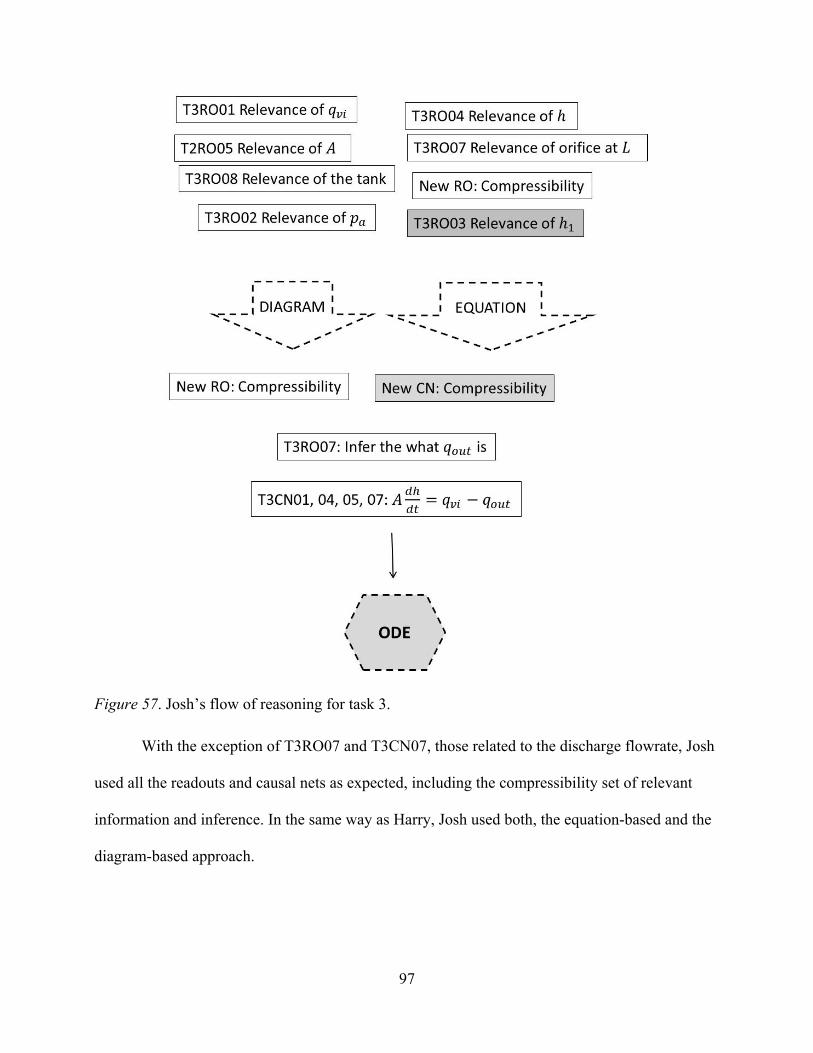
97
Figure 57. Josh’s flow of reasoning for task 3.
With the exception of T3RO07 and T3CN07, those related to the discharge flowrate, Josh
used all the readouts and causal nets as expected, including the compressibility set of relevant
information and inference. In the same way as Harry, Josh used both, the equation-based and the
diagram-based approach.
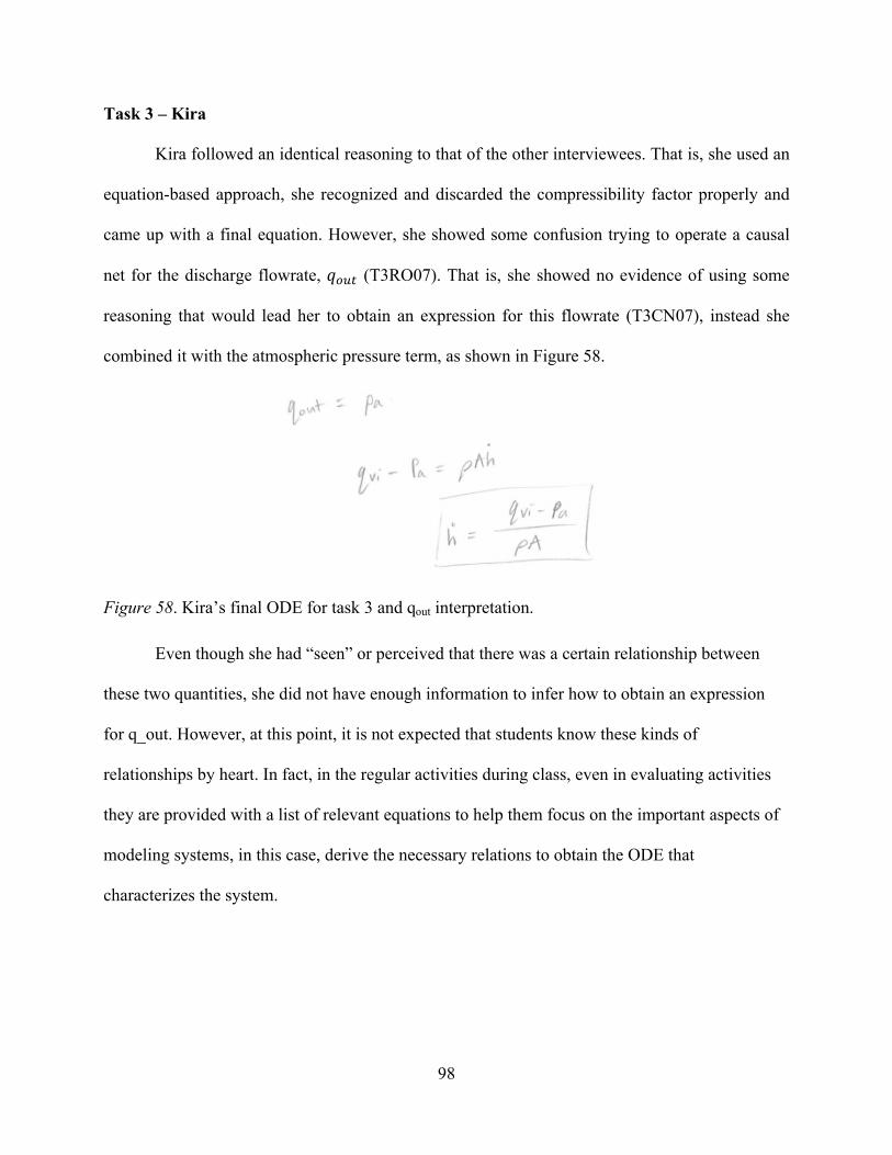
98
Task 3 – Kira
Kira followed an identical reasoning to that of the other interviewees. That is, she used an
equation-based approach, she recognized and discarded the compressibility factor properly and
came up with a final equation. However, she showed some confusion trying to operate a causal
net for the discharge flowrate, (T3RO07). That is, she showed no evidence of using some
reasoning that would lead her to obtain an expression for this flowrate (T3CN07), instead she
combined it with the atmospheric pressure term, as shown in Figure 58.
Figure 58. Kira’s final ODE for task 3 and qout interpretation.
Even though she had “seen” or perceived that there was a certain relationship between
these two quantities, she did not have enough information to infer how to obtain an expression
for q_out. However, at this point, it is not expected that students know these kinds of
relationships by heart. In fact, in the regular activities during class, even in evaluating activities
they are provided with a list of relevant equations to help them focus on the important aspects of
modeling systems, in this case, derive the necessary relations to obtain the ODE that
characterizes the system.
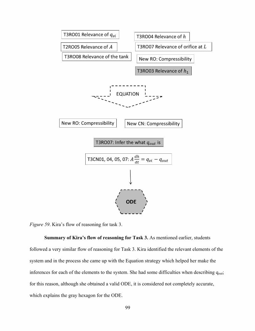
99
Figure 59. Kira’s flow of reasoning for task 3.
Summary of Kira’s flow of reasoning for Task 3. As mentioned earlier, students
followed a very similar flow of reasoning for Task 3. Kira identified the relevant elements of the
system and in the process she came up with the Equation strategy which helped her make the
inferences for each of the elements to the system. She had some difficulties when describing qout;
for this reason, although she obtained a valid ODE, it is considered not completely accurate,
which explains the gray hexagon for the ODE.

100
Summary of Results
The tables below summarize the strategies used by the students in each task, and how
close or successful they were at solving the tasks.
Table 10 presents what strategy(ies), of the three defined in the Results section, each
student used in each task. Kira was the student who tried more strategies along the solution of the
tasks compared to Zane who seemed focused on less approaches but showed better results if we
look at Table 9.. Zane successfully obtained the ODEs for tasks 1 and 3, the mechanical and fluid
system respectively. In terms of success rate, Rebecca showed the best results; as Zane she
obtained correct ODEs for tasks 1 and 3, and she partially succeeded in task 2. Harry and Josh
showed similar results, both completed task 3 and showed partial progress with task 1. On the
other hand, Kira could only show good performance in task 3. In fact, this task was the only one
in which all students successfully obtained an ODE, taking into account the limitations they had
during the interviews.
As stated in the description of the tasks in the Methods section, task 2 was meant to be a
challenging context for the students. Given that they are mechanical engineering undergraduates,
they mention this fact during the interviews, that they are not very familiar with these kinds of
contexts; however, this exercise was informative as for the analysis of the challenges they faced
when they had to apply similar principles in a novel context, which is the essence of transfer of
learning.
Going back to Table 10, Kira’s results show limitations in her abilities to solve the tasks
but at the same time, showed efforts to use as many resources as possible to make sense of the
system’s behavior and attempts to set up the ODEs; this is evidenced along the analysis of the
result of her tasks. Harry and Josh on the other hand, had little effectiveness not only in the
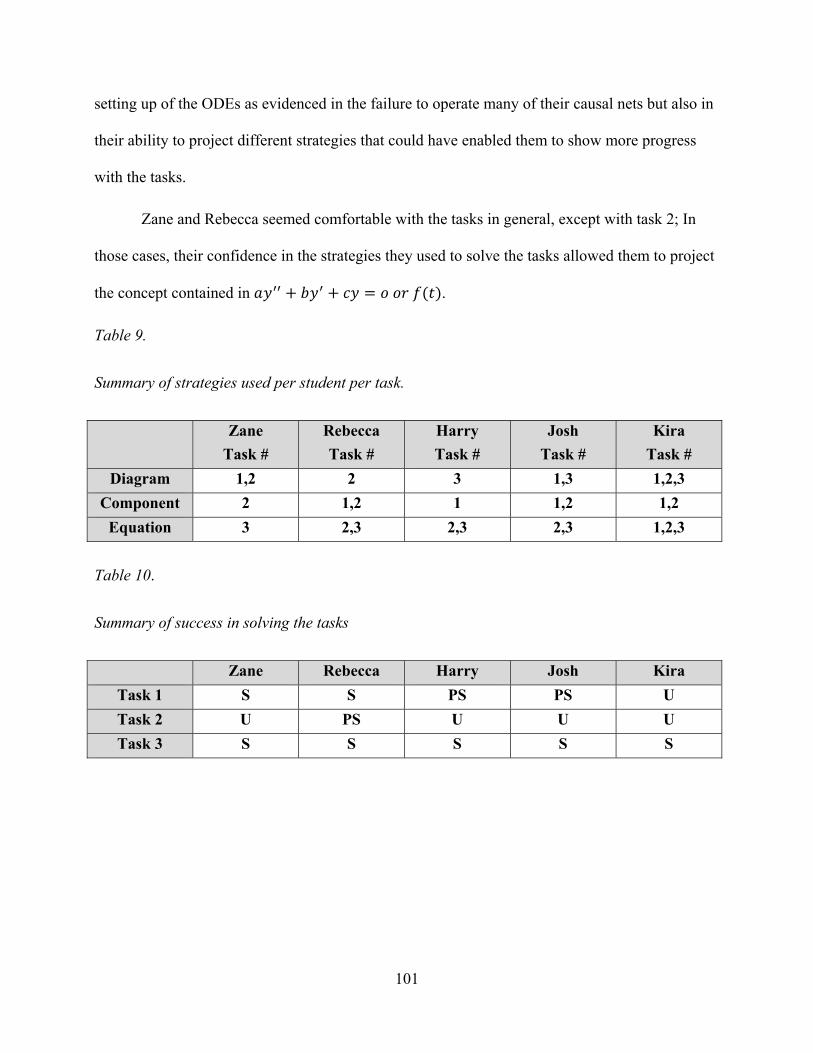
101
setting up of the ODEs as evidenced in the failure to operate many of their causal nets but also in
their ability to project different strategies that could have enabled them to show more progress
with the tasks.
Zane and Rebecca seemed comfortable with the tasks in general, except with task 2; In
those cases, their confidence in the strategies they used to solve the tasks allowed them to project
the concept contained in .
Table 9.
Summary of strategies used per student per task.
Zane
Task #
Rebecca
Task #
Harry
Task #
Josh
Task #
Kira
Task #
Diagram 1,2 2 3 1,3 1,2,3
Component 2 1,2 1 1,2 1,2
Equation 3 2,3 2,3 2,3 1,2,3
Table 10.
Summary of success in solving the tasks
Zane Rebecca Harry Josh Kira
Task 1 S S PS PS U
Task 2 U PS U U U
Task 3 S S S S S

102
CHAPTER 6: DISCUSSION
In this section I discuss the results of this study and compare them with the literature
related to studies on differential equations and the concepts of coordination class. I also discuss
about the extent to which students relied on mathematical concepts throughout the solution of the
tasks. Then, I examine in more detail the implications of the use of the strategies students used
along the tasks. I discuss the implications of this study with aspects of instruction in differential
equations and system dynamics classes. In addition, I consider the implications of this study with
respect to the transfer of learning perspective. Finally I discuss the limitations and implications of
this study for future research in mathematics education and engineering education.
Implications for the Coordination Class Theory
diSessa and Sherin (1998) estimated that it is the causal nets and not the set of readout
strategies, the core problem in learning physics concepts. In this study I have been able to
demonstrate that diSessa and Sherin’s conjecture is true; students in general were able to identify
the elements of information of the systems, even from task 2 despite its difficulty. On the other
hand, the attempts to project the concept based on the strategies identified as I analyzed students’
work seemed to be effective in some cases (Zane and Rebecca), but insufficient in others (Kira).
Besides, Harry and Josh not only were not as fluent in these strategies when compared to their
classmates; but also, the ones the used could not enable them to complete the tasks. It seems
apparent that the concept projection might not be accurate unless the student completely
understands the implications (inferences) of the elements that he/she uses to eventually obtain the
information he/she wants to obtain from a certain quantity.
Coordination class theory describes intrinsic difficulties that students face when reading
information from the world. In this study, I intended to provide students different contexts to
103
challenge students’ understanding of the principles underlying each of the systems they had to
analyze. Given that the participants were all mechanical engineering students, I assumed that they
would probably have better performance in tasks 1 and 3, mechanical and fluid respectively; the
electrical system would pose more difficulties for them. Taking this into account, I recall the
concept of span which relates to the applicability of a concept in different situations. Except by
Rebecca, all the participants were unable to articulate the concepts of ordinary differential
equations in task 2. The fact that they were unfamiliar with how the elements interacted in this
system hindered the possibility to see the differential equation that described that system’s
behavior. diSessa and Wagner (2005) argue that by partitioning the structure of the coordination
class - readouts and causal nets among others – might simplify instruction interventions. This
implies that for learning and teaching matters, coordination class theory might shed light
regarding how to help students widen their span; that is, the applicability of a concept. In this
specific case determined for this study: modeling dynamic systems through ordinary differential
equations.
Within the theory of Coordination Classes diSessa and Wagner (2005) state that
coordination clusters are defined as: “coordination classes that mutually influence each other’s
development”. The evolution of a coordination class is inherently linked to new understanding of
the concepts defining it. For example, a better understanding of the concept of force, imply new
meanings for mass and acceleration. This study included coordination clusters undoubtedly
contributes to the empirical work that has been developed in the previous years, for example
Wagner (2006) with the concepts of “expected value”, “sample” and “distribution” in his study
on the law of large numbers; or Thaden-Koch (2003) with the study on coordinating velocity.
104
Students’ Leaning on Mathematical Concepts
This study evidenced the complexity of analyzing this kind of tasks that involve concepts
from several disciplines (e.g. engineering, physics and mathematics). Our interest is mainly
focused on the mathematical aspects of the tasks, although sometimes the concepts are tightly
intertwined.
The description of the solution of the tasks from the expert’s point of view refers to
mathematical aspects from the tasks. In this paragraph I discuss how students leaned on these
aspects as they worked on the tasks. In Task 1, all of them properly recognized the relevance of
the small angle which allowed them to use simpler terms. The appearance of the variable and
its derivatives came up implicitly as the students inferred the role of each of the components of
the system. There were only brief mentions from Zane and Harry to the fact that the pendulum
mass implies the existence of a second derivative of , which then supposed the fact that the
solution of the task implied a second order differential equation. On the other hand, every student
rearranged their final expression to resemble the form of the ODE they were shown in previous
occasions because that form is potentially helpful in further stages of modeling this kind of
systems
In the case of Task 2 there is little to be mentioned with respect of the mathematical
influence to obtain the ODE for this system due to the lack of familiarity of students with this
kind of contexts. As shown in the Results section, all of them were unsuccessful at arriving to a
valid ODE representation of this system. The only student who was close to finish this task,
Rebecca, did not have the chance to think of potential tools that would help her go further with
the task. Mathematically speaking, she was close to get an expression that would eventually need
derivation and further rearrangements of the terms; however, she failed to recognize the
105
relevance of the node found after the inductor (L) and made the inferences that would have led
her to that point. On the other hand, those students who turned to use the Laplace method (a
mathematical tool) found themselves stuck in it and gave up on that strategy; which lead us to
conclude that, for this Task, there was no evidence that the mathematical tools would make an
impact in the solution of the Task.
In the case of Task 3, the most relevant aspect to note is the fact that all students obtained
the expression for by relating it to the change of the volume of the tank, which refers to that
second step cited by Blanchard et al., (1998). Also, students rearranged the final expression to
make it similar to that of a standard ODE.
In summary, if we think of modelling of dynamic systems as a whole, there are two major
stages to consider; the first implies representing a real life situation in an ODE, the second entails
solving that ODE. Taking this into account, the mathematical aspects involved in this process are
more heavily present at the second stage rather than the first one; however, there is still room for
analyzing the implications of mathematics in the first stage and this study evidences that there are
potential aspects that might shed light on the modelling process.
Students’ Strategies as Concept Projections
Earlier I described three strategies that students used to approach the tasks: Diagram-
based, Component-based and Equation-based. In this section I discuss the scope of these
strategies as well as their relation with the causal nets and readouts.
On the one hand, I argue that these strategies can be considered concept projections
because these entail a set of knowledge and plans in order to apply a certain concept in a given
context. In this manner, I found that students used these three strategies in different ways and this
use allowed them to solve the tasks. On the other hand, I consider the effect of these strategies as

106
for whether these facilitated the solution of the problems and also I make mention of what aspects
were essential to solve each of the tasks.
The diagram strategy allowed the students to visualize a holistic perspective of the task.
As the student has a big picture of the system, it is easier for him/her to identify the elements that
are playing a role in how the system behaves. This is a deduction process that allows the student
to narrow down the terms of the ODE. This strategy may not always be useful in certain contexts
and this is a weakness I identified of it. For example, the electrical system did not allow to use
this strategy effectively although, recognizing its effectiveness, some students attempted to use it.
The component-based strategy on the other hand, allowed the students to focus on the
individual elements of the system and first focus on their effect in the system to, eventually,
include it in the overall analysis. Rebecca chose to use this option in Task 1 and the main part of
her work involved focusing on the task taking into account this strategy. It is worth mentioning
that students chose to use the strategies unaware of what I currently describe in this study; that is,
they had no label or identifying way to choose among the strategies, they only decided as they
solved the tasks. This strategy had a drawback at the moment of putting together all the elements
that had already been described. In trying to solve Task 2, for example, Rebecca had come to a
valid analysis of the components, but she gave up on that strategy because she did not make the
right inference on the effect of one of the components. This last thought implies that, although a
student might be able to draw different strategies, unless he/she makes the right inferences,
he/she will be restrained as to how far he/she can work on a given task. However, in the case of
Rebecca, at least she could identify what aspect of the Task made it difficult to handle. Other
students used different strategies with similar results.

107
The equation-based strategy served well in the case of Task 3 although I presume that this
Task was easily solved using this strategy because there were a few number of elements in the
system. This strategy had the students identify the terms of the equation with their corresponding
component in the system. This seems to be a straightforward technique, but as I already
mentioned, this would not be the case if there were more elements involved.
Now, it is important to consider Kira’s case regarding the use of the strategies. She was
the student who shoed the lower results as she solved the tasks but at the same time, I argue that
it was because she was resourceful as for the use of those strategies that she could show some
progress with the tasks. On the other hand, this case confirms what I stated in the last paragraph
where I argue that no matter how many strategies are used, unless the right causal nets are
properly deployed, there will be stages of the process in which the student will just get stuck.
In contrast, I also consider it is worth mentioning Rebecca’s performance at solving Task
2. Contrary to what happened to Kira in all the Tasks (where she had no productive results), it
was the use of different strategies that allowed her to show some progress. In this case, this
evidence might prove my conjecture of the usefulness of the strategies. In Rebecca’s case, the
combination of strategies allowed to “see” that there was a key aspect in one of the elements of
the system (the inductor) that would lead her to continue with the solution of the task.
Unfortunately for her she could not go any further with the task due to the lack of inferences.
Learning Differential Equations
In the Literature review chapter I cited Blanchard et al. (1998) discussing about the steps
of the process of modeling with differential equations. Steps one involved establishing the rules
or laws that described the quantities to analyze; in step two the student defines the variables and
parameters to use in the model and the third step focuses on using those relationships between

108
quantities to obtain the equation. When compared with the coordination class theory, it is
possible to compare steps 2 with the identification of the readout strategies and steps 1 and 3 with
the operation of the causal nets. Given that Blanchard et al., and other textbooks follow a similar
pattern to approach the modeling process, this study might shed light on methodologies adopted
by authors concerning the teaching of differential equations and thus emphasize on strengthening
students’ skills in these steps.
The strategies used by the participants informed about the different ways in which a
student might approach a task involving the modeling of the differential equation of a system.
These could be assumed as concept projections of the modeling in different instances. These
concept projections facilitated to some extent the implementation of the ordinary differential
equation concept in different contexts. This study has helped identify and define the
characteristics of these projections. This idea could imply effects on the way that modeling is
taught in differential equations courses as well as engineering courses dealing with this process.
It is possible that further studies refine the definition, limitations and scope of these strategies and
thus help students in understanding and carry out modeling of systems more efficiently.
Understanding of Students’ Thinking of Differential Equations
I have also referred to Rasmussen’s framework to interpret students’ understanding and
thinking of differential equations. Although most of the theory he proposed is not applicable
within the scope of this study, I consider that it is important to make mention to a specific section
of his study with respect to part of the students’ results. In his framework, Rasmussen two themes
involving the difficulties that students usually show when reporting understanding (or the lack of
it) of differential equations. One of these themes is called: the function-as-solution dilemma
theme. In this theme, Rasmussen reports that students fail to interpret the solution of a differential
109
equation in terms of a function; they are used to finding the solution of an equation resulting in a
“number” instead of a family of functions. As the results for two of the students in task 2
involved expressions closely related to an algebraic equation than a differential equation, in this
study I have shown evidence that these issues remain in students’ thinking.
Implications for Transfer of Learning Processes
I have also mentioned that coordination class theory, as argued by diSessa and Wagner
(2005) has a structure whose elements can inform the possibility of transfer. Concept projections
and span involve enough elements to consider this theory as a valid precursor to study transfer of
learning processes. A basic conception of transfer allows a yes/no possibility of transferred
knowledge from one situation to another. In contrast, different perspectives of transfer of learning
beg the possibility to study this phenomenon from a transitional and evolving point of view. In
this study I argue that the lack of span in the context of task 2 (electrical system) could be
considered as an argument in favor to analyze transfer of learning in more detail. There were
though certain aspects, like the proper use of the readout strategies; that could evidence a partial
accomplishment of transfer in this context considering the failure in the operation of the causal
nets as stage in which the completion of the transfer process was not completed. Still, it would be
necessary to use the proper transfer of learning perspective to provide further details of the
process. Indeed, the Transfer-In-Pieces perspective (Wagner, 2006) is founded on the
coordination class theory and could provide a suitable framework in this case.
Conclusion
The research questions of this study focused on the way students applied their knowledge
in the modeling of system dynamics as well as obtaining information about the resources and
strategies they used while solving tasks. The figures showing the flow of students’ reasonings in

110
the tasks provided a possible structure of how they approached the tasks and also highlighted the
difficulties they faced at completing the tasks. On the other hand, the identification of those
strategies, the concept projections in the context of: Diagrams, Components and Equations,
offered a suitable framework upon which future studies can have some reference. Along the
Results section I showed evidence of each of these elements and provided useful information
concerning possibilities to analyze aspects of transfer of learning at undergraduate level.
111
REFERENCES
Artigue, M. (1999). The Teaching and Learning of Mathematics at University Level. Notices of
The American Mathematical Society, 46(11), 1377-1385.
Arslan, S. (2010). Traditional instruction of differential equations and conceptual learning.
Teaching Mathematics and Its Applications, 29(2), 94-107.
Bergsten, C. (2007). Investigating quality of undergraduate mathematics lectures. Mathematics
Education Research Journal, 19(3), 48-72.
Booth, S. (2008). Learning and teaching engineering mathematics for the knowledge society.
European Journal of Engineering Education, 33, 381-389.
Budinski, N. &Takaci, D. (2010). Introduction of the Notion of Differential Equations by
Modeling Based Teaching. International Journal for Technology in Mathematics
Education, 18, 107-111.
Buteler, L., Coleoni, E., & Perea, M. (2014). Aprendiendo empuje durante la resolución de
problemas: un análisis desde la Teoría de Clases de Coordinación. Ensciencias, 32(3).
https://doi.org/10.5565/rev/ensciencias.1309
Çengel, Y. & Boles, M. (2002). Thermodynamics. Boston: McGraw-Hill.
Chen, X. & Soldner, M. (2013). STEM Attrition: College Students' Paths Into and Out of STEM
Fields Statistical Analysis Report (pp. 1-10). Washington, D.C.: National Center for
Education Statistics. Retrieved from http://nces.ed.gov/pubs2014/2014001rev.pdf
Christine, M. (2007). CRS Report for Congress Science, Engineering and Mathematics
Education: Status and Issues (pp. 1-6). Washington, D.C.: Congressional Research
Service.
112
Czocher, J., Tague, J., & Baker, G. (2013). Where does the calculus go? An investigation of how
calculus ideas are used in later coursework. International Journal of Mathematical
Education in Science and Technology, 44, 673-684.
diSessa, A. A. (1993). Toward an epistemology of physics. Cognition and instruction, 10(2-3),
105-225..
diSessa, A. A. & Wagner, J. F. (2005). What coordination has to say about transfer. In J. P.
Mestre (Ed.), Transfer of learning from a modern multidisciplinary perspective (pp. 121-
154). Greenwich, CT: Information Age Publishing.
Dray, T. &Manogue, C. (2003). Using Differentials to Bridge the Vector Calculus Gap. The
College Mathematics Journal, 34, 283.
Ellis, M., Williams, B., Sadid, H., Bosworth, K. W., & Stout, L. (2004). Math usage by practicing
engineers: What does it mean to curriculum planners?. p 9, 1.
Güçler, B. (2012). Examining the discourse on the limit concept in a beginning-level calculus
classroom. Educational Studies In Mathematics, 82, 439-453.
Fox, R., Pritchard, P., McDonald, A., & Fox, R. (2011). Fox and McDonald's introduction to
fluid mechanics. Hoboken, NJ: John Wiley &Sons.
Hall, C., Dickerson, J., Batts, D., Kauffmann, P., & Bosse, M. (2011). Are We Missing
Opportunities to Encourage Interest in STEM Fields? Journal of Technology
Education, 23(1), 32-46.
Hashemi, N., Salleh Abu, M., &Kashefi, H. (2015). Designing learning strategy to Improve
Undergraduate Students' Problem Solving in Derivatives and integrals: A Conceptual

113
Framework. Eurasia Journal of Mathematics, Science and Technology Education, 11,
227-238.
Hibbeler, R. (1997). Mechanics of materials. Upper Saddle River, N.J.: Prentice Hall.
Horwitz, A. & Ebrahimpour, A. (2002). Engineering Applications in Differential and Integral
Calculus. International Journal of Engineering Education, 18, 78-88.
Hu, D. &Rebello, N. (2013). Understanding student use of differentials in physics integration
problems. Physical Review Special Topics - Physics Education Research, 9. doi:
10.1103/physrevstper.9.020108
Incropera, F. (2007). Introduction to heat transfer. Hobokenm, NJ: Wiley.
Jones, S. (2015). The prevalence of area-under-a-curve and anti-derivative conceptions over
Riemann sum-based conceptions in students’ explanations of definite integrals.
International Journal of Mathematical Education in Science and Technology, 46, 721-
736.
Jones, S. R. (2015). Areas, anti-derivatives, and adding up pieces: Integrals in pure mathematics
and applied contexts. The Journal of Mathematical Behavior, 38, 9-28
Martinez Ortiz, A. & Sriraman, V. (2015). Exploring Faculty Insights into Why Undergraduate
College Students Leave STEM Fields of Study—A Three-Part Organizational Self-Study.
American Journal of Engineering Education, 6, 43.
Orton, A. (1983). Students' understanding of differentiation. Educational Studies in Mathematics,
14(3), 235-250. doi: 10.1007/bf00410540
Palm, W. (2005). System Dynamics. Boston: McGraw-Hill Higher Education.

114
Pennell, S., Avitabile, P., &White, J. (2009). An Engineering-Oriented Approach to the
Introductory Differential Equations Course. PRIMUS, 19(1), 88-99.
Peters, M. & Kortecamp, K. (2010). Rethinking Undergraduate Mathematics Education: The
importance of classroom climate and self-efficacy on mathematics achievement. Current
Issues in Education, 13(4). Retrieved from http://cie.asu.edu/
Pilgrim, M. (2014). Addressing the Standards for Mathematical Practice in a Calculus Class.
Mathematics Teacher, 108(1), 52-57. Retrieved from
http://www.jstor.org/stable/10.5951/mathteacher.108.1.0052 doi:1
Powers, R., Craviotto, C., & Grassl, R. (2010). Impact of proof validation on proof writing in
abstract algebra. International Journal Of Mathematical Education In Science And
Technology, 41(4), 501-514.
President's Council of Advisors on Science and Technology,. (2012). Report to the President
Engage to Excel: Producing One Million Additional College Graduates with Degrees in
Science, Technology, Engineering, and Mathematics (p. i to x). Washington D.C.:
Executive Office of the President of the United States. Retrieved from
https://www.whitehouse.gov/sites/default/files/microsites/ostp/pcast-engage-to-excel-
final_2-25-12.pdf
Rasmussen, C. (2001). New directions in differential equations. The Journal of Mathematical
Behavior, 20(1), 55-87.
Raychaudhuri, D. (2013). A framework to categorize students as learners based on their cognitive
practices while learning differential equations and related concepts. International Journal
of Mathematical Education in Science and Technology, 44(8), 1239-1256.

115
Redish, E. (2005). Problem Solving and the Use of Math in Physics Courses. In World View on
Physics Education. International Physics Education Conference. Delhi.
Shipman, B. (2012). A Comparative Study of Definitions on Limit and Continuity of Functions.
PRIMUS, 22(8), 609-633.
Soon, W., Lioe, L., & McInnes, B. (2011). Understanding the difficulties faced by engineering
undergraduates in learning mathematical modelling. International Journal Of
Mathematical Education In Science And Technology, 42(8), 1023-1039.
SEFI Société Européenne pour la Formation des Ingénieurs,. (2016). A Framework for
Mathematics Curricula in Engineering Education (pp. 61-65). Brussels: European Society
for Engineering Education (SEFI). Retrieved from http://sefi.htw-
aalen.de/Curriculum/Competency%20based%20curriculum%20incl%20ads.pdf
STEM Education Statistics. (2016). National Math and Science Initiative. Retrieved from
https://www.nms.org/AboutNMSI/TheSTEMCrisis/STEMEducationStatistics.aspx
Wagner, J. (2006). Transfer in Pieces. Cognition And Instruction, 24(1), 1-71.
Wainwright, C., Morrell, P., Flick, L., & Schepige, A. (2004). Observation of Reform Teaching
in Undergraduate Level Mathematics and Science Courses. School Science and
Mathematics, 104(7), 322-335.
Willcox, K. & Bounova, G. (2004). Mathematics in Engineering: Identifying, Enhancing and
Linking the Implicit Mathematics Curriculum. In American Society for Engineering
Education Annual Conference and Exposition. American Society for Engineering
Education. Salt Lake City, Utah.