Analysis of coherent structures and atmosphere-canopy...

Atmos. Chem. Phys., 11, 11921–11936, 2011www.atmos-chem-phys.net/11/11921/2011/doi:10.5194/acp-11-11921-2011© Author(s) 2011. CC Attribution 3.0 License.

AtmosphericChemistry

and Physics

Analysis of coherent structures and atmosphere-canopy couplingstrength during the CABINEX field campaign

A. L. Steiner1, S. N. Pressley2, A. Botros3, E. Jones4, S. H. Chung2, and S. L. Edburg5

1Department of Atmospheric, Oceanic and Space Sciences, University of Michigan, Ann Arbor, MI, USA2Department of Civil and Environmental Engineering, Washington State University, Pullman, WA, USA3Department of Neuroscience, University of California, Los Angeles, CA, USA4Franklin W. Olin College of Engineering, Needham, MA, USA5Department of Geography, University of Idaho, Moscow, ID, USA

Received: 20 June 2011 – Published in Atmos. Chem. Phys. Discuss.: 26 July 2011Revised: 4 November 2011 – Accepted: 9 November 2011 – Published: 1 December 2011

Abstract. Intermittent coherent structures can be respon-sible for a large fraction of the exchange between a for-est canopy and the atmosphere. Quantifying their contri-bution to momentum and heat fluxes is necessary to in-terpret measurements of trace gases and aerosols withinand above forest canopies. The primary objective of theCommunity Atmosphere-Biosphere Interactions Experiment(CABINEX) field campaign (10 July 2009 to 9 August2009) was to study the chemistry of volatile organic com-pounds (VOC) within and above a forest canopy. In thismanuscript we provide an analysis of coherent structures andcanopy-atmosphere exchange during CABINEX to supportin-canopy gradient measurements of VOC. We quantify thenumber and duration of coherent structure events and theirpercent contribution to momentum and heat fluxes with twomethods: (1) quadrant-hole analysis, and (2) wavelet anal-ysis. Despite differences in the duration and number ofevents, both methods predict that coherent structures con-tribute 40–50 % to momentum fluxes and 44-65 % to heatfluxes during the CABINEX campaign. Contributions asso-ciated with coherent structures are slightly greater under sta-ble atmospheric conditions. By comparing heat fluxes withinand above the canopy, we determine the degree of couplingbetween upper canopy and atmosphere, and find that theyare coupled the majority of the time. Uncoupled canopy-atmosphere events occur in the early morning (4–8 a.m. lo-cal time) approximately 30 % of the time. This study con-

Correspondence to:A. L. Steiner([email protected])

firms that coherent structures contribute significantly to theexchange of heat and momentum between the canopy andatmosphere at the CABINEX site, and indicates the need toinclude these transport processes when studying the mixingand chemical reactions of trace gases and aerosols between aforest canopy and the atmosphere.

1 Introduction

Turbulent mixing is the fundamental driver in the exchangeof mass, momentum and scalars between a forest canopy andthe atmosphere (Finnigan et al., 2009; Harman and Finnigan,2008). Quantifying these turbulent processes is necessary tounderstand the surface energy budget (Oncley et al., 2007),the global carbon budget (Law et al., 2002) and the fate ofreactive trace gas species (Holzinger et al., 2005; Sorgel etal., 2011). These vertical motions are particularly relevantfor atmospheric chemistry, where highly reactive gases andaerosols may have reaction time scales on the same orderof magnitude as transport time scales (Dlugi et al., 2010;Fuentes et al., 2007).

Characterizing exchange between tall vegetation canopiesand the atmosphere is complex because the roughness el-ements generate intermittent coherent structures (Finnigan,2000). Coherent structures are defined as a distinct patternof organized turbulence with length scales on the order ofthe canopy height. They typically result from hydrodynamicinstabilities caused by large differences in horizontal windspeeds (wind shear) near the top of the canopy (Finnigan etal., 2009) and are thought to be the main driver of local-scale

Published by Copernicus Publications on behalf of the European Geosciences Union.

http://creativecommons.org/licenses/by/3.0/

11922 A. L. Steiner et al.: Analysis of coherent structures during CABINEX

counter-gradient flow (Raupach and Thom, 1981). Two pri-mary types of exchange motion can occur: (1) A relativelyslow “burst” or ejection of air from within the canopy tothe atmosphere (representing upward motion) and (2) a rel-atively fast downward motion, or “sweep”, that brings airfrom the atmosphere into the forest canopy. Coherent struc-tures have been shown to dominate the exchange between aforest canopy and the atmosphere (Brunet and Irvine, 2000;Collineau and Brunet, 1993a; Raupach et al., 1996). Previ-ous studies indicate that coherent structures are more effec-tive at transmitting scalars than momentum (Thomas and Fo-ken, 2007) and can account for 40–87 % of the total amountof sensible heat fluxes in forested regions (Barthlott et al.,2007). This suggests coherent structures could be an impor-tant factor in the analysis of chemical concentration gradi-ents and fluxes, as measured gradients are often used to in-terpret chemical and physical processes of the forest canopye.g., (Holzinger et al., 2005; Rizzo et al., 2010; Wolfe et al.,2011).

Several techniques have been developed to isolate coher-ent structure events from the background fluctuations in mo-mentum and energy fluxes including (1) quadrant-hole (Q-H)analysis (Bergstrom and Hogstrom, 1989; Finnigan, 1979;Lu and Willmarth, 1973; Raupach, 1981; Shaw et al., 1983)and (2) wavelet transform analysis (Collineau and Brunet,1993a; Gao et al., 1989; Farge, 1992). Q-H analysis is arelatively simple approach that places the fluctuating compo-nents of the horizontal and vertical velocities into quadrantsbased on whether they are positive or negative, and then usesan exclusion region or “hole-size” to eliminate small-scalemotion and isolate stronger events. Wavelet transform anal-ysis is a more complex approach that typically uses the tem-perature time series and a wavelet as an integration kernelto define a continuous wavelet transform of the time seriesto detect events. This method identifies changes in power atspecific points within a time series, which can represent thepresence of a coherent structure.

While coherent structures have been identified as signifi-cant in the micrometeorological community, very few one-dimensional or three-dimensional atmospheric models ofcanopy-atmosphere exchange directly simulate the contribu-tion of coherent structures to vertical mixing. The most sim-plistic vertical mixing parameterizations rely onK-theory,which assumes turbulent motion is analogous to moleculardiffusion and relates a vertical flux to a vertical gradientthrough the eddy diffusivity parameter (K) (Foken, 2008).More complex models build on this approach but use higherorder turbulence closure to represent turbulent fluxes (e.g.,Yamada and Mellor, 1975; Katul et al., 2004). However,to fully capture coherent structures, a simulation techniquesuch as large-eddy simulation (LES) is required. LES solvesthe spatially filtered Navier-Stokes equations and can directlysimulate coherent structures in atmospheric boundary layerflows (Moeng, 1984; Patton et al., 2001).

In this paper, we estimate and evaluate the contribution ofcoherent structures to vertical fluxes of heat and momentumwithin and above a forest canopy during a recent field cam-paign in the summer of 2009 at the University of MichiganBiological Station (UMBS). The Community Atmosphere-Biosphere Interactions Experiment (CABINEX) field studywas designed to elucidate the role of biogenic volatile or-ganic compounds (VOC) and atmospheric oxidation withinthe canopy. As part of CABINEX, physical and chemicalmeasurements were conducted at multiple heights within theforest canopy. While previous studies have evaluated turbu-lence at the UMBS AmeriFlux site (e.g., Su et al., 2008; Vil-lani et al., 2003), a detailed analysis of coherent structuresat the same spatial location and time of CABINEX chemi-cal measurements is required for interpretation of chemicalgradient measurements and other flux measurements at theUMBS facility. This description of canopy-atmosphere cou-pling can be useful in conjunction with chemical gradientmeasurements (e.g. Sorgel et al., 2011) and modeling to un-derstand the role of mixing in atmospheric chemistry studies.The UMBS experimental facility has a broad research com-munity using the site for a wide variety of flux measurements,ranging from biogenic VOC to carbon dioxide and nitrogenfluxes. Further, this work can be useful for scientists studyingatmospheric chemistry at other similar ecosystems. The goalof this paper is to identify coherent structure contributions tomixing in the forest canopy and highlight time periods whenthe canopy is coupled to the atmosphere. The use of twocoherent detection methods provides a comparison of tech-niques that is infrequently implemented in existing literature(Thomas and Foken, 2007).

2 Site and meteorological data description

2.1 Site and field campaign description

The UMBS site is located on approximately 4000 hectaresof mixed deciduous forest in northern Michigan near thecity of Pellston (45◦35′ N, 84◦42′ W). The stand age is ap-proximately 90 years old and has a mean canopy height of22.5 m (Fig. 1; see Carroll et al. (2001) for a full site de-scription). UMBS has three large atmospheric flux towers,including the Forest Accelerated Succession ExperimenT(FASET) tower installed in the fall of 2006 (Nietz, 2010),an AmeriFlux tower established in June 1998 (Baldocchi etal., 2001), and a tower for dedicated atmospheric chemistrystudies established in 1996 during the Program for Researchon Oxidants: PHotochemistry, Emissions, and Transport(PROPHET) (Carroll et al., 2001). This study utilizes datacollected at the PROPHET tower, located approximately 130m southeast of the AmeriFlux tower. The 2009 CABINEXfield campaign was an atmospheric chemistry experimentwith a focus on measuring in-canopy oxidation of biogenicVOC species and formation of aerosols. The PROPHET

Atmos. Chem. Phys., 11, 11921–11936, 2011 www.atmos-chem-phys.net/11/11921/2011/

A. L. Steiner et al.: Analysis of coherent structures during CABINEX 11923

Fig. 1. University of Michigan Biological Station (UMBS)PROPHET tower schematic as configured for CABINEX 2009.Two sonic anemometers were used for this study: “top” at 34 m(1.5 canopy height) and “mid” at 20.6 m (0.92 canopy height).

tower (Fig. 1) was equipped with physical and chemical in-strumentation extending above the tower platform (36.4 m),on the tower platform (31.2 m), in the mid-canopy (20.4 m)and near the forest floor (5 m) (see other manuscripts in thisACP special issue for more detail on specific chemical mea-surements). Data for this paper were collected using two highfrequency sonic anemometers (CSAT-3, Campbell ScientificInstruments) located at the top of the tower, 1.5 times thecanopy height (h) (34 m; 1.5 h) and within the upper portionof the canopy (20.6 m; 0.92 h). At the commencement ofthe campaign, sonic locations were selected to be above thecanopy and in the upper portion of the canopy based on theCABINEX campaign goals concerned with whole-canopyprocessing of chemical compounds and aerosols. The sonic

locations are not candidates for investigating the role of sub-canopy turbulence, and discerning the role of the sub-canopyfrom the upper canopy on chemical processing is an area offuture study. In the following work, we discuss the canopy-atmosphere exchange in the upper portion of the canopy.

2.2 Sonic anemometer data processing

Data from sonic anemometers were collected continuouslyat a rate of 10 Hz from 10 July–8 August 2009. Raw datafor each anemometer includes the three velocity components(defined here as streamwise (u), cross-streamwise (v), andvertical (w)), and temperature (T ). Additionally, 10 Hz CO2and H2O concentrations were collected at the top sonic loca-tion using an open path infrared gas analyzer (IRGA, Licor7500a). High frequency data (10 Hz) are pre-processed in30-min periods (18 000 data points per file) as follows:

1. Data points outside a specified range of the 30-minmean (± five standard deviations) are classified asnoise, removed, and replaced with the 30-min mean.These are likely due to instrument noise or other ex-ternal factors.

2. Coordinate rotation is applied, assuming a negligible30-min mean vertical velocity and a rotation of thestreamwise axis into the mean wind direction (Foken,2008).

After pre-processing, Reynolds decomposition is applied totemperature and three wind components, with each variableseparated into its mean (30-min average) component (u) andthe fluctuating component (u′). Fluxes are calculated foreach 30-min time period as an average product of the 10 Hzfluctuation components (e.g.u′w′ for the kinematic momen-tum flux andw′T ′ for kinematic heat flux). The Obukhovlength (L) is calculated to determine the atmospheric stabil-ity for each 30-min time period as:

L= −u3

∗

kg

Tw′T ′

(1)

whereu∗ is the friction velocity (m s−1), k is the von Karmanconstant,g is the gravitational constant (9.81 m s−1), T isthe average temperature, andw′T ′ the kinematic heat flux.L classifies 30-min time periods as unstable (L< 0), stable(L≥ 0), and neutral (|L| ≥ 1000, where we interpret absolutevalues greater than 1000 as approaching infinity).

2.3 Additional data filters for coherentstructure analysis

Approximately 30 days of sonic anemometer data (10 July–8August 2009) are analyzed (1410 possible 30-min periods),with specific 30-min time periods removed from the analy-sis due to: (1) missing data: incomplete records from either

www.atmos-chem-phys.net/11/11921/2011/ Atmos. Chem. Phys., 11, 11921–11936, 2011


anemometer (40 30-min periods or 2.8 % of the total), (2)rain events: any detected rain at the nearby UMBS Ameri-Flux tower (67 30-min periods, 4.8 %), (3) wind speeds: lessthan 1 m s−1 measured at the upper anemometer to removeweak wind conditions (99 30-min periods, 7.0 % ) and 4)wind direction: winds measured at the upper sonic from di-rections coming through the tower could be subject to inter-ference (winds between 125 and 165 degrees with the sonicoriented towards 325 degrees) (103 periods, 7.3 %). Afterapplying these four filters, 1152 30-min time periods (82 %of total) are available for further analysis.

3 Methods

We use two different methods to detect coherent structuresin the forest canopy: (1) quadrant-hole (Q-H) analysis and(2) wavelet analysis. These two methods are based on differ-ent fundamental principles; therefore the comparison of thesetwo methods provides insight into the detection of coherentstructures and the resulting contribution to the exchange ofenergy and mass between forest and canopy. Both methodsare described in this section, with additional details providedin the Appendix.

3.1 Quadrant-Hole (Q-H) analysis

Q-H or quadrant analysis is one of many conditionalsampling techniques used to study and describe turbulentflows (Antonia, 1981; Lu and Willmarth, 1973). It has beenapplied to study canopy turbulence in crop (Finnigan, 1979;Shaw et al., 1983; Zhu et al., 2007) and forest ecosystems(Baldocchi and Meyers, 1988; Bergstrom and Hogstrom,1989; Gardiner, 1994; Mortiz, 1989; Thomas and Foken,2007). Q-H analysis provides information about turbulentstructures by separating the fluctuating velocity components(u′ andw′) into four categories based on sign. FollowingShaw et al. (1983), the categories or quadrants are numberedconventionally:

Quadrant 1 (Q1):u′>0,w′>0 (outward interaction)

Quadrant 2 (Q2):u′<0,w′>0 (ejection or burst)

Quadrant 3 (Q3):u′<0,w′<0 (inward interaction)

Quadrant 4 (Q4):u′>0,w′<0 (sweep)

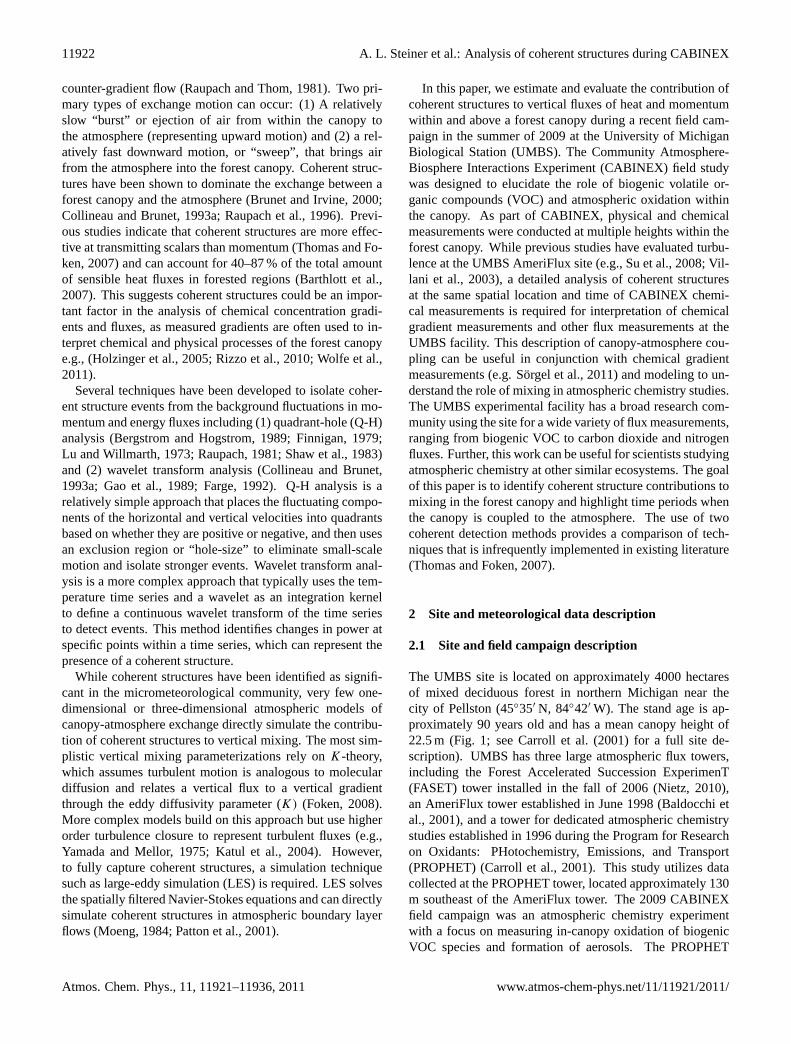
In the u′ versusw′ scatter plot in Fig. 2, events arecharacterized as a “burst” if theu′w′ is in Q2, or a “sweep”if u′w′ is in quadrant Q4. In most forested canopy studies,the sweep quadrant (Q4) is the largest contributor to mo-mentum transfer within and just above the canopy, and theejection quadrant (Q2) is the second most important contrib-utor; outward and inward interactions are also components

37

803

Figure 2. Sample 30-‐minute analysis (28 July 2009 (DOY 209), 12:30 – 13:00LT) using the 804

quadrant analysis method for different hole sizes. Each point represents a 10Hz sonic data 805

point. Note as the hole size increases weak events are excluded, thus for large hole sizes 806

(H=4) only extreme events are considered. 807

808

809

Fig. 2. Sample 30-min analysis (28 July (DOY 209), 12:30–13:00 LT) using the quadrant analysis method for different holesizes. Each point represents a 10 Hz sonic data point. Note as thehole size increases weak events are excluded, thus for large holesizes (H = 4) only extreme events are considered.

of coherent structures but lead to little exchange within aforested canopy (Finnigan, 2000).

In addition to categorizing the data by quadrant, a thresh-old parameter (Bogard and Tiederman, 1986) or hole sizeH (Lu and Willmarth, 1973) is used to separate true burstor sweep events from relatively quiescent motions (Fig. 2).Thus bursts and sweeps are detected when

u′w′ ≥H(urmswrms) (2)

where the subscript rms indicates root mean squared veloc-ity. The number and duration of events detected with Q-Hanalysis are sensitive to the threshold parameterH . Ratherthan tuneH to agree with the wavelet analysis, we used aconstantH (H = 1) for our analysis as determined by otherstudies to be a suitable threshold value (Bogard and Tieder-man, 1986; Comte-Bellow et al., 1978). Sensitivity of ourresults toH was evaluated; similar to other studies, we foundthe number of events decreases quickly with larger hole sizes(see Appendix A) (Baldocchi and Meyers, 1988; Bergstromand Hogstrom, 1989; Mortiz, 1989; Shaw et al., 1983; Zhuet al., 2007). Multiple detections occurring from the sameevent are separated from independent events using a timefrequency parameter (τ ). We selected a constant time fre-quency ofτ = 0.5 s based on analyses of several 30-min pe-riods. Additional information on the Q-H method and a sen-sitivity analysis toH andτ can be found in Appendix A.

3.2 Wavelet analysis

Past studies have successfully implemented the wavelettransform method to identify coherent structures from high-frequency turbulence data (Collineau and Brunet, 1993b;Farge, 1992; Thomas and Foken, 2005). Multiple meth-ods are available for wavelet detection of coherent structures



(Barthlott et al., 2007; Collineau and Brunet, 1993a; Feigen-winter and Vogt, 2005; Lu and Fitzjarrald, 1994; Thomasand Foken, 2005). Here we employ the method of Barthlottet al. (2007), which uses temperature fluctuations to detectramp structures under stable and unstable conditions. Weselect this method because the use of temperature ramps pro-vides a physical basis and easy visualization for the selectionof coherent structure events.

We apply wavelet analysis to the 10 Hz sonic anemometertemperature records for each 30-min period and use a “Mex-ican Hat” wavelet, which has been shown to effectively de-tect coherent structures (e.g., Collineau and Brunet, 1993a;Feigenwinter and Vogt, 2005). For each 30-min time pe-riod throughout the field campaign (1152 total periods afterpre-processing and filtering), we detect coherent structuresaccording to the following techniques defined in Barthlottet al. (2007). First, we average temperature fluctuations to1 Hz and remove any temperature trends, and then we cal-culate the wavelet transform (Wn (s)) and global waveletpower spectrum (W s) over a range of scales or periods (s)

for each 30-min time interval (see Appendix B for defini-tions and detailed methodology). We determine the period ortime scale that produces the clearly defined local maximumin W s. Then, the wavelet coefficient that corresponds to thismaximum period is used to identify coherent structures basedon known differences in temperature fluctuations and rampstructures under stable and unstable conditions (Barthlott etal., 2007). Duration of individual events is calculated fromthe beginning and end times determined above. A samplewavelet analysis that highlights these detection steps is dis-played in Fig. B1.

4 Results and discussion

After a brief description of the CABINEX campaign char-acteristics (Sect. 4.1), the two coherent structure detectionmethods are examined over the duration of the CABINEXcampaign by comparing statistics on the number and dura-tion of events (Sect. 4.2), and the contribution from coher-ent structures to fluxes of momentum and heat (Sect. 4.3).Because each method uses fundamentally different detec-tion criteria, a side-by-side comparison of the resulting fluxcontributions can provide CABINEX collaborators with arange of estimates of the contribution of coherent structuresto canopy mixing for use in future analyses of chemical andaerosol measurements. Lastly, we compare kinematic heatfluxes between the top and mid-level sonic to determine thedegree of coupling between the upper forest canopy and at-mosphere (Sect. 4.4).

4.1 CABINEX campaign characteristics

Averaged temperature (T ), wind speed (u) and friction ve-locity (u∗) derived from the top sonic anemometer data are

Table 1. Statistics of coherent structure detection for the CAB-INEX campaign, indicating the distribution function median (withstandard deviation in parentheses).

Wavelet Q-H

Number of structures

Stable 9.1 (4.9) 300.1 (81.2)Unstable 5.6 (2.8) 237.5 (49.6)

Duration of structures (s)

Stable 115.6 (39.6) 1.8 (0.4)Unstable 90.6 (38.1) 1.3 (0.3)

Momentum flux contribution (%)

Stable 48.3 (17.3) 43.2 (6.7)Unstable 39.9 (15.6) 45.3 (7.1)

Heat flux contribution (% )

Stable 47.5 (16.4) 64.5 (22.0)Unstable 44.2 (16.0) 60.5 (15.7)

Momentum transport efficiency

Stable 1.3 (1.3) 2.1 (0.3)Unstable 1.1 (1.2) 1.9 (0.3)

Heat transport efficiency

Stable 1.3 (1.4) 3.0 (1.5)Unstable 1.2 (1.3) 2.5 (1.1)

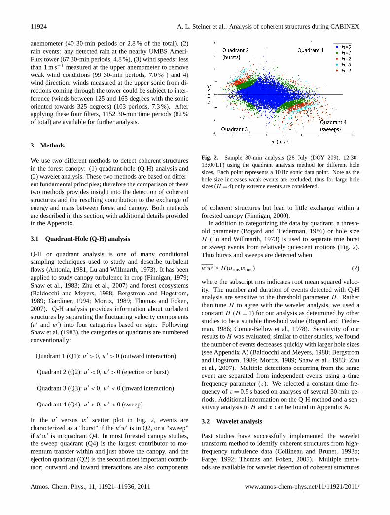
shown for the entire CABINEX campaign (Fig. 3). Air tem-peratures measured above the canopy during the campaignare relatively low for the UMBS site compared to averageair temperatures in other summers (Bertman et al., 2010)and range between 285–297 K (12–24◦C). Diurnal temper-ature ranges of up to 10 K occur throughout the campaign,although some periods have warmer nights and reduced tem-perature ranges (e.g., 22–28 July 2009 or day of year (DOY)203–209). Wind speeds range from calm to 5 m s−1, withsome periods of strong diurnal wind speed variation and oth-ers with very little diurnal variation (DOY 203–209). Liketemperature, friction velocity provides a good visual trace forthe diurnal variations during the campaign, with values rang-ing from 0–1.2 m s−1. As with temperature and wind speed,relatively low magnitudes of friction velocity (< 0.5 m s−1)

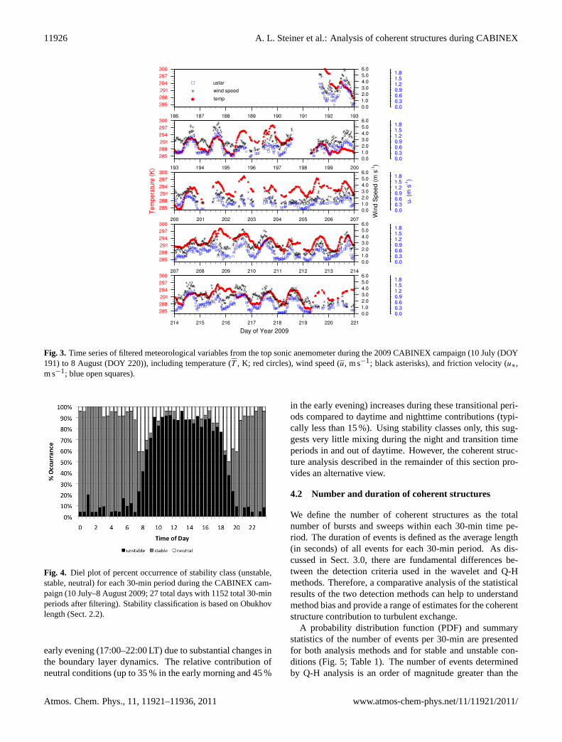
occur during the DOY 203–209 time period.Stability for each 30-min time period is determined by

Eq. (1) and a diel plot is shown in Fig. 4. Depending ondata availability after filtering (Sect. 2.3), each bar repre-sents 21 to 27 data points (e.g., days). During the campaign,sunrise is at approximately 05:00–05:30 LT and sunset at ap-proximately 20:00–20:30 LT. As expected, stable conditionsdominate during the nighttime (22:00–06:00 LT) and char-acterize 80–90 % of the nighttime 30-min periods. Unsta-ble conditions occur 70–90 % of the time during the day-time (10:00–17:00 LT). All three stability classes occur dur-ing transition periods in the morning (06:00–10:00 LT) and



38

810

Figure 3. Time series of filtered meteorological variables from the top sonic anemometer 811

during the 2009 CABINEX campaign (10 July (DOY 161) to 8 August (DOY 220)), including 812

temperature (

€

T , K; red circles), wind speed (

€

u , m s-‐1; black asterisks), and friction velocity 813

( *u , m s-‐1; blue open squares). 814

815

Fig. 3. Time series of filtered meteorological variables from the top sonic anemometer during the 2009 CABINEX campaign (10 July (DOY191) to 8 August (DOY 220)), including temperature (T , K; red circles), wind speed (u, m s−1; black asterisks), and friction velocity (u∗,m s−1; blue open squares).

39

Figure 4. Diel plot of percent occurrence of stability class (unstable, stable, neutral) for 816

each 30-‐minute period during the CABINEX campaign (10 July-‐ 8 August 2009; 27 total 817

days with 1152 total 30-‐minute periods after filtering). Stability classification is based 818

on Obukhov length (Section 2.2). 819

820

821

Fig. 4. Diel plot of percent occurrence of stability class (unstable,stable, neutral) for each 30-min period during the CABINEX cam-paign (10 July–8 August 2009; 27 total days with 1152 total 30-minperiods after filtering). Stability classification is based on Obukhovlength (Sect. 2.2).

early evening (17:00–22:00 LT) due to substantial changes inthe boundary layer dynamics. The relative contribution ofneutral conditions (up to 35 % in the early morning and 45 %

in the early evening) increases during these transitional peri-ods compared to daytime and nighttime contributions (typi-cally less than 15 %). Using stability classes only, this sug-gests very little mixing during the night and transition timeperiods in and out of daytime. However, the coherent struc-ture analysis described in the remainder of this section pro-vides an alternative view.

4.2 Number and duration of coherent structures

We define the number of coherent structures as the totalnumber of bursts and sweeps within each 30-min time pe-riod. The duration of events is defined as the average length(in seconds) of all events for each 30-min period. As dis-cussed in Sect. 3.0, there are fundamental differences be-tween the detection criteria used in the wavelet and Q-Hmethods. Therefore, a comparative analysis of the statisticalresults of the two detection methods can help to understandmethod bias and provide a range of estimates for the coherentstructure contribution to turbulent exchange.

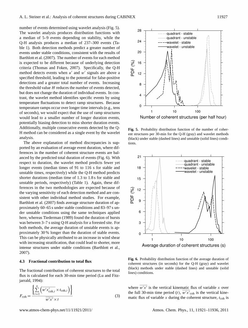
A probability distribution function (PDF) and summarystatistics of the number of events per 30-min are presentedfor both analysis methods and for stable and unstable con-ditions (Fig. 5; Table 1). The number of events determinedby Q-H analysis is an order of magnitude greater than the



number of events determined using wavelet analysis (Fig. 5).The wavelet analysis produces distribution functions witha median of 5–9 events depending on stability, while theQ-H analysis produces a median of 237–300 events (Ta-ble 1). Both detection methods predict a greater number ofevents under stable conditions, consistent with the results ofBarthlott et al. (2007). The number of events for each methodis expected to be different because of underlying detectioncriteria (Thomas and Foken, 2007). Specifically, the Q-Hmethod detects events whenu′ andw′ signals are above aspecified threshold, leading to the potential for false-positivedetections and a greater total number of events. Increasingthe threshold valueH reduces the number of events detected,but does not change the duration of individual events. In con-trast, the wavelet method identifies specific events by usingtemperature fluctuations to detect ramp structures. Becausetemperature ramps occur over longer time intervals (e.g., tensof seconds), we would expect that the use of ramp structureswould lead to a smaller number of longer duration events,potentially biasing detection to miss shorter duration events.Additionally, multiple consecutive events detected by the Q-H method can be considered as a single event by the waveletanalysis.

The above explanation of method discrepancies is sup-ported by an evaluation of average event duration, where dif-ferences in the number of coherent structure events are bal-anced by the predicted total duration of events (Fig. 6). Withrespect to duration, the wavelet method predicts fewer yetlonger events (median times of 91 to 116 s for stable andunstable times, respectively) while the Q-H method predictsshorter durations (median time of 1.3 to 1.8 s for stable andunstable periods, respectively) (Table 1). Again, these dif-ferences in the two methodologies are expected because ofthe varying sensitivity of each detection method and are con-sistent with other individual method studies. For example,Barthlott et al. (2007) finds average structure duration of ap-proximately 60–65 s under stable conditions and 83–97 s un-der unstable conditions using the same techniques appliedhere, whereas Tiederman (1989) found the duration of burstswas between 3–7 s using Q-H analysis for a forested site. Forboth methods, the average duration of unstable events is ap-proximately 30 % longer than the duration of stable events.This can be physically attributed to an increase in wind shearwith increasing stratification, that could lead to shorter, moreintense structures under stable conditions (Barthlott et al.,2007).

4.3 Fractional contribution to total flux

The fractional contribution of coherent structures to the totalflux is calculated for each 30-min time period (Lu and Fitz-jarrald, 1994):

Fcoh=

{n∑i=1

(w′x′

coh,i× tcoh,i

)}w′x′ × t

(3)

40

822

Figure 5. Probability distribution function of the number of coherent structures per 30-‐823

minute for the Q-‐H (gray) and wavelet methods (black) under stable (dashed lines) and 824

unstable (solid lines) conditions. 825

826

Fig. 5. Probability distribution function of the number of coher-ent structures per 30-min for the Q-H (gray) and wavelet methods(black) under stable (dashed lines) and unstable (solid lines) condi-tions.

41

827

Figure 6. Probability distribution function of the average duration of coherent structures 828

(in seconds) for the Q-‐H (gray) and wavelet (black) methods under stable (dashed lines) 829

and unstable (solid lines) conditions. 830

831

Fig. 6. Probability distribution function of the average duration ofcoherent structures (in seconds) for the Q-H (gray) and wavelet(black) methods under stable (dashed lines) and unstable (solidlines) conditions.

wherew′x′ is the vertical kinematic flux of variablex overthe full 30-min time period (t), w′x′

coh is the vertical kine-matic flux of variablex during the coherent structure,tcoh is



42

832

Figure 7. Probability distribution function of percentage of (a) contribution to kinematic 833

momentum flux and (b) contribution to kinematic heat flux, (c) momentum transport 834

efficiency, and (d) heat transport efficiency for the Q-‐H (gray lines), and wavelet methods 835

(black lines) under stable (dashed) and unstable (solid lines) conditions. 836

837

Fig. 7. Probability distribution function of(a) percent contribution to kinematic momentum flux,(b) percent contribution to kinematic heatflux, (c) momentum transport efficiency, and(d) heat transport efficiency for the Q-H (gray lines) and wavelet (black lines) methods understable (dashed) and unstable (solid lines) conditions.

the duration of the coherent structure, andn is the numberof events during the 30-min time period. For each method(wavelet and Q-H), we calculate the fractional contributionof the coherent structures to the kinematic momentum flux(Fm, u′w′) and kinematic heat flux (Fh, w′T ′). We also as-sess the relative efficiency (E) of these contributions by nor-malizingFcoh to the percentage of time they occupy withineach half-hour period (TC) (Barthlott et al., 2007):

TC=

n∑i=1tcoh,i

t(4)

E=Fcoh

TC(5)

Values ofE greater than one indicate that the structures aremore efficient at transporting heat or momentum, with in-creasingE values indicating greater efficiency.

The wavelet and Q-H methods yield similar fractional fluxcontributions of 40–48 % to totalFm from coherent struc-tures (Fig. 7a and Table 1).Fm contributions are slightlyhigher under stable conditions in the wavelet analysis, andslightly lower under stable conditions in the Q-H analysis.

As noted above, this is likely due to an increase in the gen-eration of structures with increasing stratification. In gen-eral, the Q-H analysis shows a narrower distribution than thewavelet analysis similar to the number and duration of events(Figs. 5 and 6), yet the resulting median values are similar.The efficiency of these structures for momentum transport(Fig. 7c) varies between the two methods, with greater effi-ciency by the Q-H method (median value of approximately2). The median efficiency for the wavelet method is slightlygreater than one (1.1 for unstable conditions and 1.3 for sta-ble conditions), yet some structures can be up to four timesas efficient as averaged fluxes as evidenced by the large stan-dard deviation. For both methods, efficiencies are greater un-der stable than unstable conditions, which may be indicativeof the increased importance of these structures under strati-fied conditions.

For Fh, the wavelet method shows a similarFcoh as forFm, with a median contribution of approximately 40–50 %(and with a similar standard deviation) and slightly greatercontributions under stable conditions. The Q-H analysis in-dicates a slightly greater contribution of coherent structuresto the kinematic heat flux, with median values of approx-imately 60–65 %. Standard deviation values and a slight



increase in contributions under stable conditions are simi-lar to the wavelet analysis. Efficiencies of kinematic heatflux are similar to the momentum transport efficiencies forthe wavelet method, but are greater than momentum fluxesfor the Q-H method. Both methods indicate that heat trans-port efficiencies are greater under stable conditions. This re-sult is consistent with Barthlott et al. (2007), who found thatthe coherent structures were slightly more efficient in theirtransport of heat than momentum. The relative contributionof coherent structures to heat or momentum transport is stillunresolved in the literature; for example, some studies showthat the contributions are roughly equal (Gao et al., 1989; Luand Fitzjarrald, 1994), others indicate that momentum fluxesare higher (Bergstrom and Hogstrom, 1989), and others sug-gest that the heat flux contribution is greater (Barthlott et al.,2007; Collineau and Brunet, 1993b; Feigenwinter and Vogt,2005). Reasons why coherent structures may differ in theirtransport of heat and momentum are uncertain, yet have im-plications for atmospheric chemistry.Fh and the eddy diffu-sivity for heat (Kh) are generally used as a proxy for otherscalar transport, and we could expect that coherent structuresmight contribute slightly more to the exchange of gases andaerosols. Despite similar magnitude of flux contributions, thetwo methods presented here show conflicting results on thecontributions to kinematic heat versus momentum flux.Fmcontributions are similar for both methods andFh contribu-tions show an increase with Q-H analysis over wavelet anal-ysis. This is consistent with the transport efficiencies, wheremomentum and heat efficiencies are similar in the waveletanalysis and greater for heat than momentum in the Q-Hanalysis, suggesting that these differences may be methoddependent.

Overall, the flux contributions using each method are sim-ilar despite the differences in the methods implemented toidentify and classify coherent structures. That is, the Q-H analysis method detects more frequent, shorter and moreefficient events while the wavelet method detects less fre-quent, longer events that are only slightly more efficient attransporting fluxes than non-events. Resulting flux contribu-tions from each method are likely similar because coherent-structure contributions are dominated by very large eventsthat are likely detected by both methods. Finnigan (1979)and Shaw et al. (1983) found that half of the total contribu-tion to momentum flux from sweeps comes from events whenu′w′>10|u′w′|; i.e., events so large that they are likely to bedetected by either method. Thomas and Foken (2007) com-pared the wavelet analysis and Q-H analysis and found thatthey can produce fundamentally different results, and favoredwavelet analysis for identifying specific event times and lo-cations. However, our findings at the CABINEX site suggestthat the flux contribution estimates are not sensitive to the de-tection method yet the Q-H method estimates more efficientcoherent structures than the wavelet method.

4.4 Canopy-atmosphere coupling strength

In CABINEX, measurements from two anemometers areavailable to determine the degree of upper canopy-atmosphere coupling, as in (Thomas and Foken, 2007). Wecompare kinematic heat flux above the canopy (Htot,1.5 h)

and the kinematic heat flux measured within the uppercanopy (Htot,0.92 h). Positive ratios suggest that the fluxesare moving in the same direction and indicate coupling be-tween the canopy and atmosphere. Following Thomas andFoken (2007), we use the relationship betweenHtot,1.5 handHtot,0.92 h to define a “strength” threshold for canopy-atmosphere coupling. A regression between these two fluxesabove a minimum value of 0.2 (Htot ≥ 0.2 K m s−1; signify-ing a substantial value) yields a slope of 0.68 (Fig. 8), and theinverse of the high flux slope (1/0.68 = 1.47) determines thethreshold of coupling between canopy and atmosphere. If theratio ofHtot,1.5 h/Htot,0.92 h is greater than zero and below thethreshold, then the canopy and atmosphere are considered tobe “strongly coupled,” as the magnitude of fluxes are rela-tively similar. If the ratio exceeds the threshold value and ispositive, then the flux of heat is in the same direction yet theflux above canopy is much stronger than the in-canopy flux.This suggests a “weakly coupled” canopy and atmosphere.Negative ratios indicate opposing flux direction and suggestthe canopy is uncoupled from the atmosphere.

The canopy and atmosphere tend to be either strongly orweakly coupled over the duration of the CABINEX cam-paign (Fig. 9). Between 10:00–18:00 LT, the canopy andatmosphere are almost always coupled, with strongly cou-pled conditions occurring 56 % of the time and weakly cou-pled conditions occurring 42 % of the time. During thenight (22:00–04:00 LT),Htot,1.5 h /Htot,0.92 h suggests that thecanopy is still coupled to the atmosphere with strong andweak conditions occurring 68 % and 27 % of the time. Thereare several instances of uncoupled conditions throughout thediurnal cycle, predominantly in the early morning (04:00–09:00 LT). The greatest instance of uncoupled conditions oc-curs at 08:00 LT, which occurs 30 % of the time over the fullcampaign period. This analysis of the diurnal cycle suggeststhat coupling occurs between the canopy and atmospheremost of the time, with early morning hours leading to thegreatest number of uncoupled conditions.

Figure 10 identifies the coupling conditions over the fulltime period of the CABINEX campaign. This time serieshighlights the dominance of strong and weakly coupled con-ditions identified in Fig. 9, and also identifies specific dayswhen uncoupled conditions occur in the early morning. Thisfigure can provide guidance for other CABINEX participantson the vertical mixing in the upper portion of the canopy andidentify time periods of strong mixing.



5 Conclusions

We present an analysis of the contribution of coherent struc-tures to vertical fluxes of heat and momentum during theCABINEX campaign 10 July to 8 August 2009 at the Uni-versity of Michigan Biological Station. Two techniques, thequadrant-hole analysis and the wavelet analysis, were usedto identify the contribution of coherent structures to fluxesof momentum and heat between the canopy and the atmo-sphere. While the two methods represent fundamentally dis-parate ideas about how coherent structures can be detected,they demonstrate that the contribution of these structures toturbulent canopy exchange is 40–48 % of the kinematic mo-mentum flux and 44–65 % of the kinematic heat flux. Wealso identify time periods of uncoupled, weakly coupled, orstrongly coupled canopy-atmosphere relationships during thecampaign, which can highlight specific time periods of well-mixed canopy-atmosphere air. The upper canopy and atmo-sphere are coupled the majority of the campaign period, how-ever, uncoupled canopy-atmosphere events occur in the earlymorning (04:00–08:00 LT) approximately 30 % of the time.

There are an increasing number of field campaigns con-ducting atmospheric chemistry gradient measurements atmultiple levels throughout the forest canopy, often withoutsupport from micrometeorologists. While prior micrometeo-rological studies have performed coherent structure analysisfor contributions to fluxes and canopy-atmosphere couplinganalysis (e.g., Thomas and Foken, 2007), there has been lit-tle interaction with the atmospheric chemistry community.The results presented here provide an example of how thesetechniques can be applied to explain mixing within the forestcanopy, a key element for understanding atmospheric chemi-cal gradients within and above forest canopies. The implica-tions of this increased vertical mixing on atmospheric chem-istry are explored in a separate paper in this Special Issue(Bryan et al., 2011), which will incorporate the impacts ofvertical mixing on modeled gradients of atmospheric con-stituents.

Current atmospheric chemistry models do not includeany method to assess coherent structures, and typically relyon traditionalK-theory to explain mixing within a forestcanopy. One exception is the use of large-eddy simulation(LES) models, which capture some of these types of canopy-atmosphere exchange (Edburg, 2009; Patton et al., 2001; Yueet al., 2007), yet these models are rarely coupled with fullchemical modeling due to computational constraints. Our re-sults show that the coherent structures will likely contributesignificantly to the canopy-atmosphere mixing during mostperiods. Somewhat counter intuitive to traditional stabil-ity analysis, coherent structures continue to play a role intransport at night which leads to coupled canopy-atmosphereconditions, a process missed by most atmospheric chemistrymodels.

We suggest future atmospheric chemistry field campaignsinclude multiple levels of meteorological measurements

43

838

Figure 8. Scatter plot of the coherent structure contribution to kinematic heat flux (Htot) 839

between the two heights (top; 1.5h and mid; 0.92h). The black line represents the slope of 840

total heat flux greater than 0.2 K m s-‐1. 841

842

Fig. 8. Scatter plot of the coherent structure contribution to kine-matic heat flux (Htot) between the two heights (top; 1.5 h and mid;0.92 h). The black line represents the slope of total heat flux greaterthan 0.2 K m s−1.

44

Figure 9. Number of occurrences of strongly coupled, weakly coupled, or uncoupled 843

atmosphere-‐canopy over the time period of the campaign (time period as in Figure 4). 844

845

Fig. 9. Number of occurrences of strongly coupled, weakly cou-pled, or uncoupled atmosphere-canopy over the time period of thecampaign (time period as in Fig. 4).

within and above canopies as well as numerical model-ing. The CABINEX campaign utilized data from two sonicanemometers, though clearly more information about thesub-canopy and in-canopy coupling is needed (Thomas andFoken, 2007). We note here that this analysis uses sonic datafrom the upper portion of the canopy, and therefore does notreflect the full coupling between the understory and the atmo-sphere. Further instrumentation in future studies would berequired to assess the below canopy coupling. These exper-imental designs are needed to quantify the role of in-canopychemical processing and exchange and separate sub-canopyprocesses from the upper canopy.



45

846

Figure 10. Time series of coupling over the duration of the campaign (black closed 847

circles). Friction velocity (red open circles) is shown for reference. 848

849

Fig. 10. Time series of coupling over the duration of the campaign (black closed circles). Friction velocity (red open circles) is shown forreference.

Appendix A

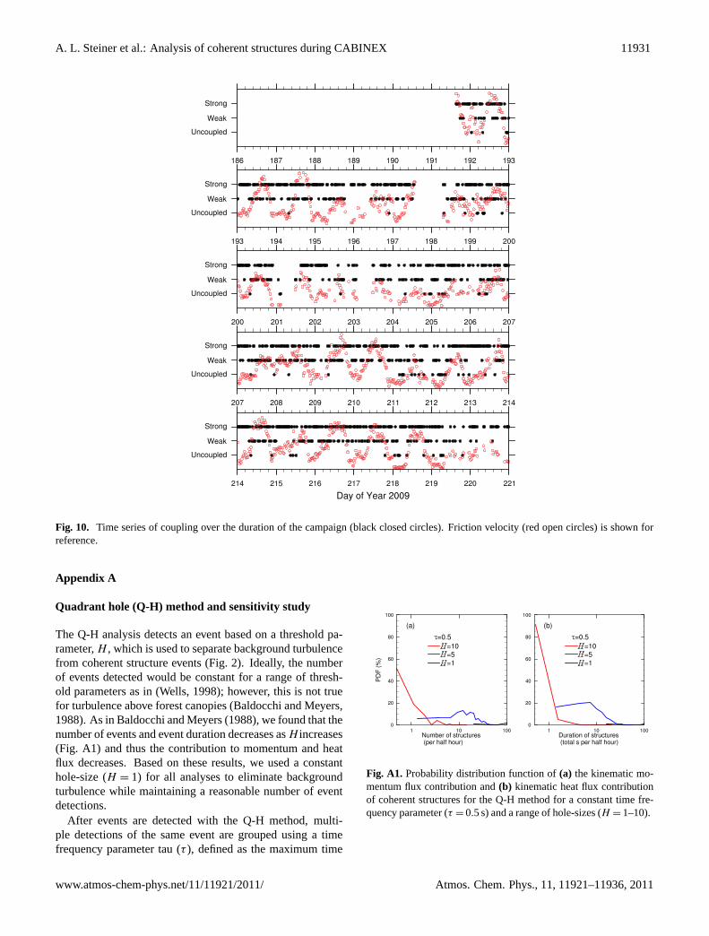
Quadrant hole (Q-H) method and sensitivity study

The Q-H analysis detects an event based on a threshold pa-rameter,H , which is used to separate background turbulencefrom coherent structure events (Fig. 2). Ideally, the numberof events detected would be constant for a range of thresh-old parameters as in (Wells, 1998); however, this is not truefor turbulence above forest canopies (Baldocchi and Meyers,1988). As in Baldocchi and Meyers (1988), we found that thenumber of events and event duration decreases asH increases(Fig. A1) and thus the contribution to momentum and heatflux decreases. Based on these results, we used a constanthole-size (H = 1) for all analyses to eliminate backgroundturbulence while maintaining a reasonable number of eventdetections.

After events are detected with the Q-H method, multi-ple detections of the same event are grouped using a timefrequency parameter tau (τ ), defined as the maximum time

Fig. A1. Probability distribution function of(a) the kinematic mo-mentum flux contribution and(b) kinematic heat flux contributionof coherent structures for the Q-H method for a constant time fre-quency parameter (τ = 0.5 s) and a range of hole-sizes (H = 1–10).



47

856

Figure A2. Sample histogram (left axis) and cumulative probability distribution (right 857

axis) of time between ejections (TE (s)) for a single 30-‐minute time period (07: 30 LT on 19 858

July 2009). The time frequency parameter, τ, can be estimated by the minimum in the 859

histogram or the intersections of the two asymptotic lines in the plot of the cumulative 860

probability distribution on a logarithmic scale against TE (Luchik and Tiederman, 1987; 861

Tiederman, 1989). 862

863

Fig. A2. Sample histogram (left axis) and cumulative probabilitydistribution (right axis) of time between ejections (TE (s)) for a sin-gle 30-min period (07:30 LT on 19 July 2009).τ , the maximumtime between ejections of the same burst event, can be estimated bythe minimum in the histogram or the intersections of the two asymp-totic lines in the plot of the cumulative probability distribution on alogarithmic scale againstTE (Luchik and Tiederman, 1987; Tieder-man, 1989).

between ejections from the same burst.τ is obtained byplotting the histogram or cumulative probability function ofthe time between events and visually detecting two distinctlydifferent statistical regions: a region of multiple ejectionswithin a single burst, and a region of independent detectionsfrom different bursts (Luchik and Tiederman, 1987; Tieder-man, 1989) (Fig. A2). We conducted this analysis for sev-eral half hour periods spanning multiple days during CAB-INEX, and found a range ofτ between 0.3 to 1.5 s. We thenconducted a sensitivity study on a range ofτ (Fig. A3) andfound the variation in both number of structures and durationof structures using the range ofτ values is low. Therefore,we used a constantτ = 0.5 s for all periods in the CABINEXanalysis.

Appendix B

Wavelet analysis and sensitivity tests

Wavelet analysis is a method frequently employed to detectcoherent structures (Collineau and Brunet, 1993b; Gao et al.,19891; Kumar and Foufoula-Georgiou, 1994; Thomas andFoken, 2007). Application of wavelet analysis to canopy-scale turbulence can depict variations of power within a timeseries, where sharp changes in power at specific points inthe time series represent the presence of a coherent structure.This provides additional information as compared to Fouriertransforms, which analyze variations of power yet lose thetime component of the analysis.

48

864

Figure A3. Probability distribution function of (a) the number of coherent structures 865

and (b) the average duration of coherent structures (seconds) for the Q-‐H method for a 866

constant hole-‐size (H = 1) and a range of time frequency parameters (τ = 0.3-‐1.5 s). 867

868

Fig. A3. Probability distribution function of(a) the number of co-herent structures and(b) the average duration of coherent structures(seconds) for the Q-H method for a constant hole-size (H = 1) anda range of time frequency parameters (τ = 0.3−1.5 s).

The wavelet method defines a continuous wavelet trans-form Wn (s) for a variablex(t) (e.g., temperature) using awaveletψ(t) as an integration kernel (Kumar and Foufoula-Georgiou, 1994):

Wn(s)=1

s

∫∞

−∞

x(t)9

(t−n

s

)(B1)

wherenis a position translation,sis a scale dilation, and thewaveletψ(t) is a real or complex-valued function with zeromean (Barthlott et al., 2007). The scale dilation,s, allowsthe broadening or narrowing ofψ(t), andn shifts the time oftheψ(t) origin. By changings over a time series, the ampli-tude and scale of turbulence can be visualized (Torrance andCampo, 1998). The wavelet variance (also called the globalwavelet spectrum;W s) yields the integrated energy content ata specifics, providing a representative scale of the coherentstructures and corresponding to the mean structure duration.

As noted in Sect. 3.2 we employ the Barthlott et al. (2007)method of wavelet analysis and coherent structure detection.This specific detection technique uses temperature fluctu-ations to detect ramp structures under stable and unstableconditions. We employ the “Mexican Hat” wavelet to de-tect ramps (Collineau and Brunet, 1993a; Feigenwinter andVogt, 2005), because the second derivative of the signal cre-ates a change in sign at discontinuities in a similar manner astemperature ramps (Barthlott et al., 2007). For each 30-mintime period throughout the field campaign, we detect coher-ent structures according to the following steps:

1. Average temperature perturbations to 1 Hz and detrendeach 30-min time period (Fig. B1a);

2. Calculate the wavelet function (Fig. B1b) and waveletpower spectrum (Fig. B1c) for each 30-min time period;

3. Determine the period that produces the greatest power,by finding a clearly defined local maximum in the global



49

869

Figure B1. Sample wavelet analysis for a single 30-‐minute period (14:30 LT on 28 July 870

2009) based on the Barthlott et al., (2007) detection method. (a) Temperature 871

perturbation from the mean (K), (b) Wavelet period versus time, (c) Global wavelet 872

spectrum, with the peak power (red dot), which selects the power for the wavelet 873

spectrum for this half hour, and (d) plot of temperature perturbation (T’; black line), 874

vertical wind perturbation (w’; gray line), wavelet (blue line), and detected burst 875

periods (w’ positive; red shaded regions) and sweep periods (w’ negative; blue shaded 876

regions). 877

Fig. B1.Sample wavelet analysis for a single 30-min period (14:30 LT on 28 July 2009) based on the Barthlott et al. (2007) detection method.(a) Temperature perturbation from the mean (K),(b) Wavelet period versus time,(c) Global wavelet spectrum, with the peak power (red dot),which selects the power for the wavelet spectrum for this half hour, and(d) plot of temperature perturbation (T ′; black line), vertical windperturbation (w′; gray line), wavelet (blue line), and detected burst periods (w′ positive; red shaded regions) and sweep periods (w′ negative;blue shaded regions).

50

878 Figure B2. Sensitivity analysis of wavelet technique to the wavelet power spectrum 879

threshold criteria of 40% (black; used in the paper analysis), 30% (blue) and 50% (red) 880

for the (a) number of coherent structures, (b) duration of structures, and (c) percent 881

contribution to total heat flux. 882

883

Fig. B2.Sensitivity analysis of wavelet technique to the wavelet power spectrum threshold criteria of 40 % (black; used in the paper analysis),30 % (blue) and 50 % (red) for the(a) number of coherent structures,(b) duration of structures, and(c) percent contribution to kinematicheat flux.

wavelet spectrum (Barthlott et al., 2007; red dot inFig. B1c).

4. Identify the coherent structures based on known differ-ences in temperature fluctuations and ramp structuresunder stable and unstable conditions (Barthlott et al.,2007). Stable-condition ramp structures have a sharpincrease in temperature followed by a slow decrease(black line; Fig. B1d), and can be detected by a zero-

crossing of the global wavelet spectrum, followed bylocal maximum, followed by a local minimum in thewave function (blue line; Fig. B1d). Unstable-conditionramp structures have a slow increase in temperature fol-lowed by a sharp drop (Barthlott et al., 2007), and un-stable and neutral time periods are detected by a seriesof local minimum in the global wavelet power spec-trum, followed by local maximum, followed by a zero-crossing of the wave function. For a local maximum to



be considered a defined peak, it has to reach a positivevalue at or greater than 40 % of the maximum value forthat wave function in the 30-min time period, therebyeliminating small peaks and fluctuations (Barthlott etal., 2007; Collineau and Brunet, 1993a).

5. Identify the direction of the coherent structure basedon the averagew′ value within the specific structure(Fig. B1d; grey line) (e.g., aw′ greater than zero in-dicates a burst, while aw′ less than zero indicates asweep). For further ease of visual analysis of thesestructures, coherent structure time intervals designatedas bursts are shaded red and sweeps are shaded blue.

Over the full campaign, these analysis steps are repeated foreach 30-min time period to identify the number of coherentstructures and their duration. Statistics for the full campaignare presented in Figs. 5 and 6.

The wavelet analysis results are insensitive to the selec-tion of s and time interval (t), but do exhibit slight sensitivityto the 40 % cutoff criteria (Fig. B2). Decreasing (increas-ing) the criteria by±10 % decreased (increased) the numberof structures detected per half hour, leading to a decrease (in-crease) of contribution of coherent structures to the kinematicheat flux by shifting the median value by approximately 5 %.While this can make slight differences in the contributionnumbers, the conclusion that coherent structures contributeto the kinematic heat flux remains robust.

Acknowledgements.We gratefully acknowledge the entire CAB-INEX team, led by S. Bertman, M.A. Carroll, P. Shepson andP. Stevens for their logistical support and assistance. We alsothank C. S. Vogel of UMBS for providing precipitation datafrom the AmeriFlux tower. Wavelet analysis was possible dueto software provided by C. Torrence and G. Compo (available athttp://atoc.colorado.edu/research/wavelets). Funding for this workwas provided by the National Science Foundation ATM-0904128to A. L. Steiner at the University of Michigan (UM) and ATM-0904214 to S. N. Pressley and S. H. Chung at Washington StateUniversity (WSU). Additional support was also provided throughthe Research Experience for Undergraduates (REU) program atUM to support A. Botros (ATM-0552353) and WSU to supportE. Jones (ATM-0754990), and through the Biosphere AtmosphereResearch and Training NSF IGERT program to support S. L.Edburg.

Edited by: J. Fuentes

References

Antonia, R. A.: Conditional sampling in turbulence measurements,Annu. Rev. Fluid Mech., 13, 131–156, 1981.

Baldocchi, D. D. and Meyers, T. P.: Turbulence structure in a de-ciduous forest, Bound-Lay. Meteorol., 43, 345–364, 1988.

Baldocchi, D. D., Falge, E., Gu, L., Olson, R., Hollinger, D.,Running, S., Anthoni, P., Bernhofer, C., Davis, K., Evans, R.,Fuentes, J., Goldstein, A., Katul, G., Law, B., Lee, X., Malhi, Y.,Meyers, T., Munger, W., Oechel, W., Paw U., K. T., Pilegaard,K., Schmid, H. P., Valentini, R., Verma, S., Vesala, T., Wilson,K., and Wofsy, S.: FLUXNET: A New Tool to Study the Tempo-ral and Spatial Variability of Ecosystem-Scale Carbon Dioxide,Water Vapor and Energy Flux Densities, B. Am. Meteorol. Soc.,82, 2415–2435, 2001.

Barthlott, C., Drobinski, P., Fesquet, C., Dubos, T., and Pietras, C.:Long-term study of coherent structures in the atmospheric sur-face layer, Bound.-Lay. Meteorol., 125, 1–24, 10.1007/s10546-007-9190-9, 2007.

Bergstrom, H. and Hogstrom, U.: Turbulent exchange above a for-est, II: Organized structures, Bound.-Lay. Meteorol., 49, 231–263, 1989.

Bertman, S. B., Carroll, M. A., Shepson, P. B., and Stevens, P. S.:Overview of CABINEX/PROPHET 2009, Fall Meeting, Amer-ican Geophysical Union, San Francisco, CA, Abstract A53C–0234, 2010.

Bogard, D. G. and Tiederman, W. G.: Burst detection with single-point velocity measurements, J. Fluid. Mech., 162, 389–413,1986.

Brunet, Y. and Irvine, M. R.: The control of coherent eddies invegetation canopies: Streamwise structure spacing, canopy shearscale and atmospheric stability, Bound.-Lay. Meteorol., 94, 139–163, 2000.

Bryan, A. M., Forkel, R., Bertman, S. B., Carroll, M. A., Dusan-ter, S., Edwards, G. D., Griffith, S., Guenther, A. B., Hansen,R. F., Jobson, T., Keutsch, F. N., Lefer, B. L., Pressley, S. N.,Shepson., P. B., Stevens, P. S., and Steiner, A. L.: In-canopygas-phase chemistry during the 2009 CABINEX field campaign:Sensitivity to isoprene chemistry and vertical mixing, in prepa-ration, 2011.

Carroll, M. A., Shepson, P. B., and Bertman, S. B.: Overview ofthe Program for Research on Oxidants: Photochemistry, Emis-sions and Transport (PROPHET) Summer 1998 measurementsintensive, J. Geophys. Res.-Atmos., 106, 24275–24288, 2001.

Collineau, S. and Brunet, Y.: Detection of turbulent coherent mo-tions in a forest canopy, 1. Wavelet analysis, Bound.-Lay. Mete-orol., 65, 357–379, 1993a.

Collineau, S. and Brunet, Y.: Detection of turbulent coherent mo-tions in a forest canopy, Part 2: Time-scales and conditional av-erages, Bound.-Lay. Meteorol., 66, 49–73, 1993b.

Comte-Bellow, G., Sabot, J., and Saleh, I.: Detection of intermittantevents maintaining Reynolds stress, Proc. Dynamic Flow Conf.– Dynamic Measurements in Unsteady Flows, 1978.

Dlugi, R., Berger, M., Zelger, M., Hofzumahaus, A., Siese, M.,Holland, F., Wisthaler, A., Grabmer, W., Hansel, A., Koppmann,R., Kramm, G., Mollmann-Coers, M., and Knaps, A.: Turbulentexchange and segregation of HOx radicals and volatile organiccompounds above a deciduous forest, Atmos. Chem. Phys., 10,6215–6235,doi:10.5194/acp-10-6215-2010, 2010.

Edburg, S.: A numerical study of turbulence, dispersion and chem-istry within and above forest canopies, Ph.D., College of Engi-neering and Architecture, Washington State University, Pullman,2009.

Farge, M.: Wavelet transforms and their applications to turbulence,Annual Reviews of Fluid Mechanics, 24, 395–457, 1992.


http://atoc.colorado.edu/research/wavelets

http://dx.doi.org/10.5194/acp-10-6215-2010


Feigenwinter, C. and Vogt, R.: Detection and analysis of coherentstructures in urban turbulence, Theor. Appl. Climatol., 81, 219–230, 2005.

Finnigan, J.: Turbulence in plant canopies, Annu. Rev. Fluid Mech.,32, 519–571, 2000.

Finnigan, J. J.: Turbulence in waveing wheat: II. Structure of mo-mentum transfer, Bound.-Lay. Meteorol., 16, 213–236, 1979.

Finnigan, J. J., Shaw, R. H., and Patton, E. G.: Turbulence structureabove a vegetation canopy, J. Fluid Mech., 637, 387–424, 2009.

Foken, T.: Micrometeorology, Springer-Verlag, Berlin, 306 pp.,2008.

Fuentes, J. D., Wang, D., Bowling, D. R., Potosnak, M., Monson,R. K., Goliff, W. S., and Stockwell, W. R.: Biogenic hydrocarbonchemistry within and above a mixed deciduous forest, J. Atmos.Chem., 56, 165–185, 2007.

Gao, W., Shaw, R. H., and Paw U, K. T.: Observation of organizedstructure in turbulent flow within and above a forest canopy,Bound.-Lay. Meteorol., 47, 349–377, 1989.

Gardiner, B.: Wind and wind forests in a plantation spruce forest,Bound.-Lay. Meteorol., 67, 161–186, 1994.

Harman, I. N. and Finnigan, J. J.: Scalar concentration profiles inthe canopy and roughness sublayer, Bound.-Lay. Meteorol., 129,323–351, 2008.

Holzinger, R., Lee, A., Paw, K. T., and Goldstein, U. A. H.: Ob-servations of oxidation products above a forest imply biogenicemissions of very reactive compounds, Atmos. Chem. Phys., 5,67–75,doi:10.5194/acp-5-67-2005, 2005.

Katul, G. G., Mahrt, L., Poggi, D., and Sanz, C.: One- and twoequation models for canopy turbulence, Bound.-Lay. Meteorol.,113, 81–109, 2004.

Kumar, P. and Foufoula-Georgiou, F.: Wavelet analysis in geo-physics: An introduction, in: Wavelets in Geophysics, editedby: Foufoula-Georgiou, E. and Kumar, P., Academic Press, SanDiego, 372 pp., 1994.

Law, B. E., Falge, E., Gu, L., Baldocchi, D. D., Bakwin, P.,Berbigier, P., Davis, K., Dolman, A. J., Falk, M., Fuentes, J. D.,Goldstein, A., Granier, A., Grelle, A., Hollinger, D., Janssens, I.A., Jarvis, P., Jensen, N. O., Katul, G., Mahli, Y., Matteucci, G.,Meyers, T., Monson, R., Munger, W., Oechel, W., Olson, R., Pi-legaard, K., Paw, K. T., Thorgeirsson, H., Valentini, R., Verma,S., Vesala, T., Wilson, K., and Wofsy, S.: Environmental con-trols over carbon dioxide and water vapor exchange of terrestrialvegetation, Agric. For. Meteorol., 113, 97–120, 2002.

Lu, C.-H. and Fitzjarrald, D. R.: Seasonal and diurnal variations ofcoherent structures over a deciduous forest, Bound.-Lay. Meteo-rol., 69, 43–69, 1994.

Lu, S. S. and Willmarth, W. W.: Measurements of the structure ofthe Reynolds stress in a turbulent boundary layer, J. Fluid Mech.,60, 481–511, 1973.

Luchik, T. S. and Tiederman, W. G.: Timescale and structure ofejections and bursts in turbulent channel flows, J. Fluid Mech.,174, 529–552, 10.1017/S0022112087000235, 1987.

Moeng, C.-H.: A large-eddy simulation model for the study of plan-etary boundary-layer turbulence, J. Atmos. Sci., 45, 3573–3587,1984.

Mortiz, E.: Heat and momentum transport in an oak forest canopy,Bound.-Lay. Meteorol., 49, 317–329, 1989.

Nietz, J. G.: Soil respiration during partial canopy senescence in anorthern mixed deciduous forest, M.S., Ecology and Organismal

Biology, The Ohio State University, 110 pp., 2010.Oncley, S. P., Foken, T., Vogt, R., Kohsiek, W., DeBruin, H. A.

R., Bernhofer, C., Christen, A., van Gorsel, E., Grantz, D.,Feigenwinter, C., Lehner, I., Liebethal, C., Liu, H., Mauder, M.,Pitacco, A., Ribeiro, L., and Weidinger, T.: The Energy Bal-ance Experiment EBEX-2000. Part I: Overview and energy bal-ance, Bound.-Lay. Meteorol., 123, 1–28,doi:10.1007/s10546-007-9161-1, 2007.

Patton, E. G., Davis, K., Barth, M. C., and Sullivan, P. P.: Decayingscalars emitted by a forest canopy: A numerical study, Bound.-Lay. Meteorol., 100, 91–129, 2001.

Raupach, M. R.: Conditional statistics of Reynold’s stress in roughwall and smooth wall turublent boundary layers, J. Fluid Mech.,108, 363–382, 1981.

Raupach, M. R. and Thom, A. S.: Turbulence in and above plantcanopies, Annu. Rev. Fluid Mech., 13, 97–129, 1981.

Raupach, M. R., Finnigan, J. J., and Brunet, Y.: Coherent eddiesand turbulence in vegetation canopies: The mixing-layer anal-ogy, Bound.-Lay. Meteorol., 78, 351–382, 1996.

Rizzo, L. V., Artaxo, P., Karl, T., Guenther, A. B., and Greenberg,J.: Aerosol properties, in-canopy gradients, turbulent fluxes andVOC concentrations at a pristine forest site in Amazonia, Atmos.Environ., 44, 503–511, 2010.

Shaw, R. H., Tavangar, J., and Ward, D. P.: Structure of Reynoldsstress in a canopy layer, J. Clim. Appl. Meteorol., 22, 1922–1931, 1983.

Sorgel, M., Trebs, I., Serafimovich, A., Moravek, A., Held, A., andZetzsch, C.: Simultaneous HONO measurements in and abovea forest canopy: influence of turbulent exchange on mixing ratiodifferences, Atmos. Chem. Phys., 11, 841–855,doi:10.5194/acp-11-841-2011, 2011.

Su, H.-B., Schmid, H. P., Vogel, C. S., and Curtis, P. S.: Effectsof canopy morphology and thermal stability on mean flow andturbulence statistics observed inside a mixed hardwood forest,Agr. For. Meteorol., 148, 862–882, 2008.

Thomas, C. and Foken, T.: Detection of long-term coherent ex-change over spruce forest using wavelet analysis, Theor. Appl.Climatol., 80, 91–104,doi:10.1007/s00704-004-0093-0, 2005.

Thomas, C. and Foken, T.: Flux contribution of coherent struc-tures and its implications for the exchange of energy and matterin a tall spruce canopy, Bound.-Lay. Meteorol., 123, 317–337,10.1007/s10546-006-9144-7, 2007.

Tiederman, W. G.: Eulerian detection of turbulent bursts, NearWall Turbulence, Proc. Z. Zoriac Memorial conference, 874–447, 1989.

Torrance, C. and Campo, G. P.: A practical guide to wavelet analy-sis, B. Am. Meteorol. Soc., 79, 61–78, 1998.

Villani, M. G., Schmid, H. P., Su, H.-B., Hutton, J. L., and Vogel, C.S.: Turbulence statistics measurements in a northern hardwoodforest, Bound.-Lay. Meteorol., 108, 343–364, 2003.

Wells, B. E.: Atmospheric boundary layer bursting: the fundamen-tal mechanism of particle entrainment, Mechanical Engineering,Pullman, Washington State University, 80 pp., 1998.

Wolfe, G. M., Thornton, J. A., Bouvier-Brown, N. C., Goldstein, A.H., Park, J.-H., McKay, M., Matross, D. M., Mao, J., Brune, W.H., LaFranchi, B. W., Browne, E. C., Min, K.-E., Wooldridge,P. J., Cohen, R. C., Crounse, J. D., Faloona, I. C., Gilman, J.B., Kuster, W. C., de Gouw, J. A., Huisman, A., and Keutsch,F. N.: The Chemistry of Atmosphere-Forest Exchange (CAFE)



http://dx.doi.org/10.1007/s10546-007-9161-1

http://dx.doi.org/10.1007/s10546-007-9161-1



http://dx.doi.org/10.1007/s00704-004-0093-0


Model – Part 2: Application to BEARPEX-2007 observations,Atmos. Chem. Phys., 11, 1269–1294,doi:10.5194/acp-11-1269-2011, 2011.

Yamada, T. and Mellor, G.: A simulation of the Wangara boundarylayer data, J. Atmos. Sci., 32, 2309–2329, 1975.

Yue, W. S., Meneveau, C., Parlange, M. B., Zhu, W. H.,van Hout, R., and Katz, J.: A comparative quadrant analy-sis of turbulence in a plant canopy, Water Resour. Res., 43,doi:10.1029/2006WR005583, 2007.

Zhu, W., van Hout, R., and Katz, J.: PIV measurements in the atmo-spheric boundary layer within and above a mature corn canopy.Part II: Quadrant-hole analysis, J. Atmos. Sci., 64, 2825–2838,2007.




http://dx.doi.org/10.1029/2006WR005583

Analysis of coherent structures and atmosphere-canopy...

Documents

Transcript of Analysis of coherent structures and atmosphere-canopy...