Analysis of BRITE data —a cookbook

Version 1.6

Andrzej Pigulskipigulski@astro.uni.wroc.pl

June 14, 2015

1 Preamble

The first data from five working BRITE nanosatellites have been sent to users. It is thereforetime to start analysis and make science. A few months ago, BEST1 decided on the pipelinewhich will be used2 for reduction of all BRITE data, after choosing from those that weredeveloped by the PHOTT3 members. The choice was preceded by an evaluation processundertaken by several people including the undersigned. Working with BRITE photometryallowed me to gain some experience and learn the characteristics of the data. For this reason,I was asked to write the first version of a kind of cookbook, i.e. this document. However,the document reflects the experience of many people that were involved in the work withBRITE data, especially the members of PHOTT. The document is intended to help those whostart their work with BRITE photometry. Since this is the beginning of our work with BRITEdata, it is clear that this document will be frequently updated. I invite all interested partiesto contribute to these updates.

There is no single best way to work with any data and BRITE data is not an excep-tion. The comments given below should be therefore regarded only as hints, not as the onlypossible way to proceed. In general, working with BRITE data requires some amount ofinteraction and flexibility. Although I have a script4 which can be run to produce the finalresult in a minute or so, I typically run it several times because I need to see some interme-diate plots to decide on the optimal parameters. The proposed procedure is therefore ratheriterative and interactive.

The present version of the cookbook refers to the second data release (hereafter DR2),now available for the first six observed fields (Ori, Cen, Sgr, Cyg, Ori-II, and Per). Thedifference between DR2 and the first data release (hereafter DR1) is the format of the data:DR2 has extended information in the header and two new columns; a column with JD and anaperture flag. On the other hand, a column with heliocentric time correction present in DR1

1BRITE Executive Science Team.2The current pipeline, developed by Dr. Adam Popowicz, is based on aperture photometry with constant,

circular aperture optimized for each star and satellite and observational setup. There is one exception: forchopping data (see below) non-circular apertures are used. The only correction to the measured fluxes is thecorrection for intra-pixel variability approximated by a fourth-order polynomial. Further improvements of thepipeline and related data releases are, however, considered for the future.

3PHOtometry Tiger Team.4Presently with 14 parameters.

1

haS been dropped now. If you still work with DR1 files, refer to Ver. 1.5 of the cookbook,please. Both DR1 and DR2 are based on the same aperture photometry with a constantaperture radius. In addition to the ‘standard’ aperture photometry, DR2 includes resultsfrom observations made in so called chopping mode (see Sect. 3 for more explanations) notavailable in DR1.

The DR1 data were made available to users in February 2015 (for Ori and Cen fields),April 2015 (for Sgr and Cyg fields) and May 2015 (for Ori-II and Per fields). DR2 data for allsix fields were made available to users in June 2015.

2 A few words on BRITEs

Before we start a description of the analysis of BRITE photometry, a few words should besaid about the instrument(s) and problems encountered during reduction. The set of BRITEnanosatellites is called BRITE-Constellation and consists of five working5 low-orbit satelliteslaunched in 2013 and 2014. Some characteristics of the BRITEs are given in Table 1.

Table 1: BRITE satellites

Satellite Abbr. Filter Launch date Porb [min] Comments

BRITE-Austria (A) BAb blue 25.02.2013 100.36UniBRITE (A) UBr red 25.02.2013 100.37Lem (PL) BLb blue 21.11.2013 99.57BRITE-Montreal (CA) BMb blue 19.06.2014 — lost, tungsten shieldBRITE-Toronto (CA) BTr red 19.06.2014 98.24 tungsten shieldHeweliusz (PL) BHr red 19.08.2014 97.10 4-lens optics, boron shield

Additional information on the satellites can be found on the BRITE-Constellation webpage6, BRITE Photometry Wiki7, and in the technical paper by Weiss et al. (2014, PASP 126,573). Due to the limitations of telemetry, a pre-selection of targets in an observed 25-degwide field-of-view is first carried out. Except for the commissioning phase, no full imagesare dowloaded; instead, rasters8 around selected bright stars are stored and downloaded toground stations. The images are intentionally defocused to avoid saturation and to decreasesensitivity of photometry to pixel-to-pixel sensitivity variations. Sample images are shownin Fig. 1.

Already at the beginning of our work with BRITE images it was obvious that their re-duction won’t be a trivial task. The main factors that pose problems in observations andreductions are the following:

(A) The number of hot (and associated but weaker cold) pixels and other chip defects (badcolumns) is large and growing with time. This is mostly a result of bombardment ofthe detectors by cosmic-ray protons. In the lack of effective shielding, they cause chipdefects.

5The sixth BRITE, Canadian BRITE-Montreal (BMb), did not separate from the upper stage of the launcherfor unknown reason.

6http://www.brite-constellation.at7http://brite.craq-astro.ca/doku.php?id=start8The size of a raster depends on the field, star, satellite and way of observing.

2

Figure 1: The rasters for 15 stars observed in the Orion field by BAb (left) and UBr (right). Therasters have size of 32 × 32 pixels. Note different shapes of the same stars for the two satellites.Image courtesy Rainer Kuschnig.

(B) Although satisfying mission requirements, the tracking is sometimes not ideal, whichresults in a permanent wobbling of a star in a raster. In some images, stars even fallpartially beyond the raster, making such images inappropriate for aperture photom-etry. The drift of stars may cause considerable smearing even in 1-s exposures. Thismay be the most severe factor diminishing the quality of BRITE photometry.

(C) In some regions of the BRITE detectors, an additional defect called charge transferinefficiency (CTI) occurs. CTIs cause additional smearing. CTIs are caused by shal-low incidence of cosmic-ray protons, while hot pixels are mainly the result of moreperpendicular incidence, depending also on the proton energy.

All three factors degrade the final photometry. A lot of effort was aimed at minimizing theirinfluence. First of all, when the problem was first recognized, four BRITEs were still notlaunched. It was therefore decided to shield the detectors in three of them (BMb, BTr andBHr). Observations indicate that the shielding is most effective in BHr, where different op-tics allowed for more space to place the shielding behind the detector. A boron shield wasmounted in this place. On the other hand, Adam Popowicz proposed a new way of observ-ing (called chopping). It is based on a combination of alternate shifts of a star’s position ina raster and subtraction of consecutive images. The first tests show that this method pro-vides better photometry than a standard pipeline. Consequently, this method of observingis used whenever possible. The first BRITE data based on chopping mode of observing aredelivered in DR2 for the Perseus field.

Up to now, data for the following fields have been made available for users: (1) 1 OrionI-2013 (BAb & UBr), (2) 2 Centaurus-2014 (BAb, UBr, BTr & BLb), (3) 3 Sagittarius-2014 (UBr),(4) 4 Cygnus-2014 (BAb, UBr & BTr), (5) 5 Perseus-2014 (BAb & UBr + chopping with UBr),and (6) 6 Orion-II-2014 (BAb, BLb, BTr & BHr). Location of the BRITE fields (completed,ongoing and planned till the mid-2016) in the sky is presented in Fig. 2.

3

OriOri-II

CenSgr

Cyg

Per

completed (observed stars are marked red)

Vel/Pupβ PicSco

ongoing

Cyg-II

Cas/Cep CMa/Pup

Cru/Car

Sgr-II

planned

BRITE fields(Galactic coordinates, Aitoff projection, stars brighter than V = 6 mag)

Figure 2: Location of BRITE fields in the sky. The curved line is the celestial equator.

3 Chopping mode of observation

Following the recognition of a serious problem with the increasing number of hot pixels,Adam Popowicz proposed a new way of observing called now chopping. In choppingmode, consecutive images are taken with alternate shifts that move stars from their nom-inal positions within a raster in one direction, forth and back. Next, a pair of consecutiveimages is subtracted and the photometry is performed on difference images. For obviousreasons, rasters in the chopping mode are rectangles not squares as in the standard mode.An example of a series of two consecutive images obtained in chopping mode and the re-sulting difference image is shown in Fig. 3.

Figure 3: An example of observations in the chopping mode. The right-hand image is the imagewhich is used for photometry. Note that very few hot pixels can be seen in it. Images courtesy AdamPopowicz.

4

The photometry in chopping mode is still aperture photometry, but the apertures arenow non-circular. They are derived by means of thresholding a series of stellar images and— once derived — consequently applied to all images. In addition, the contribution frompixels falling partially into aperture is taken into account.

4 BRITE data files

The BRITE data are sent to users as ASCII files separately for each BRITE satellite, observedfield and observational setup.9 The files contain a header section followed by a data sectionin the form of seven columns. The header includes all important information on the satellite,observed field, observational setup, etc. The header records start with the letter ‘c’. The datasegment contains seven columns; the column entries are explained in the bottom part of theheader. A sample beginning of a data file is shown in Fig. 4.

Figure 4: Beginning of a sample BRITE DR2 data file.

The sixth columns contain Julian Day (JD) which can be used to identify the correspond-ing image.10 Note that data sets do not contain information on the uncertainty in flux level.Since some fitting programs require uncertainties, I will show later how to derive and addsuch values to data files.

The photometry in chopping mode comes as a single setup file. However, the photom-etry was made on a star in two different positions in a CCD. Given the lack of flat-fielding,this may result in an offset between the photometry made on images in one position withrespect to the other one. Before starting the analysis I would therefore suggest splitting thechopping-mode photometry into two subsets, depending on the position of a star in the

9The observational setups can differ because of: different raster sizes, stacking or non-stacking data, chop-ping or normal way of observing, different exposure times, etc. Because each difference may lead to somenon-identical systematic effects, data are sent separately for each setup. Eventually, they can or even should becombined, but one may want to correct for the systematic effects first.

10JDs are used as file names of raw images.

5

raster. This can be easily done using data in column 3 or 4 containing stellar centres ofgravity, xcen and ycen, respectively. I am writing ‘3 or 4’ because in chopping mode bothdirections of movement were used. Figure 5 shows an example of ycen for a star observed inchopping mode — the position fall in two different ranges. Using them the data can easilyseparated into two subsets.

Figure 5: The ycen values for UBr chopping data of HD 19058 (ρ Per).

5 Before time-series analysis

First, you need to decide whether you want to work with fluxes or magnitudes. This isabsolutely up to you and — in principle — both choices are equally good. Personally, I preferto work with magnitudes, so I start with converting fluxes to magnitudes. In addition, theworking file should not have a header, so I remove it. In some data files I found ‘NaN’ (not anumber) entries — these lines need to be removed, too. All this can be done using standardshell commands.11. The first part of my script looks like this (the starting ‘>’ is a terminalprompt, ‘lc.data’ is a working file name, ‘lc.tmp’ is a temporary file name):

> cp [original file name] lc.data

> grep -v c lc.data > lc.tmp; mv lc.tmp lc.data

> grep -i -v nan lc.data > lc.tmp; mv lc.tmp lc.data

> awk ’{printf("%13.8lf %12.7lf %7.2lf %7.2lf %7.2lf %s\n",$1−2456000.0,−2.5*log($2)/log(10.0)+14.5,$3,$4,$5,$7)}’ lc.data > lc.tmp;

mv lc.tmp lc.data

The last awk command shows that I also subtract 2456000.0 from the HJD and add an ar-bitrary constant of 14.5 to the derived magnitudes, i.e. magnitude = −2.5 log (flux) + 14.5.Of course you can stay with fluxes. After this procedure, a single record in the working filelc.data looks like this (the column with JD is omitted):

820.81283769 2.0928448 14.13 13.29 15.83 1

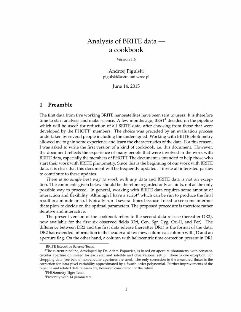
This is something you may want to plot. Again, use your favourite plotting tool (my choiceis Gnuplot12) to see this. You may see something like the light curve shown in Fig. 6. It

11I am using a laptop with Mac OS X Yosemite system, but the commands can be used practically as they arein any Linux-type system. Of course, you can do the same in any way with your favourite system and commandor program(s).

12http://gnuplot.sourceforge.net

6

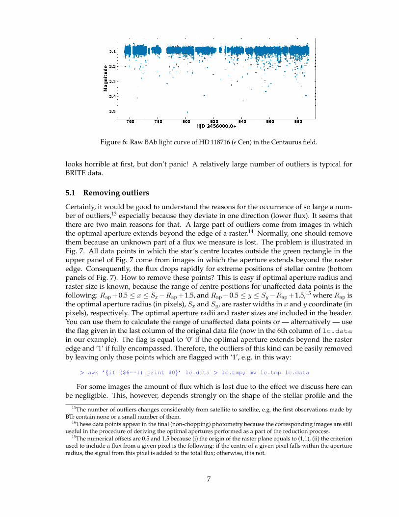
Figure 6: Raw BAb light curve of HD 118716 (ε Cen) in the Centaurus field.

looks horrible at first, but don’t panic! A relatively large number of outliers is typical forBRITE data.

5.1 Removing outliers

Certainly, it would be good to understand the reasons for the occurrence of so large a num-ber of outliers,13 especially because they deviate in one direction (lower flux). It seems thatthere are two main reasons for that. A large part of outliers come from images in whichthe optimal aperture extends beyond the edge of a raster.14 Normally, one should removethem because an unknown part of a flux we measure is lost. The problem is illustrated inFig. 7. All data points in which the star’s centre locates outside the green rectangle in theupper panel of Fig. 7 come from images in which the aperture extends beyond the rasteredge. Consequently, the flux drops rapidly for extreme positions of stellar centre (bottompanels of Fig. 7). How to remove these points? This is easy if optimal aperture radius andraster size is known, because the range of centre positions for unaffected data points is thefollowing: Rap+0.5 ≤ x ≤ Sx−Rap+1.5, andRap+0.5 ≤ y ≤ Sy−Rap+1.5,15 whereRap isthe optimal aperture radius (in pixels), Sx and Sy, are raster widths in x and y coordinate (inpixels), respectively. The optimal aperture radii and raster sizes are included in the header.You can use them to calculate the range of unaffected data points or — alternatively — usethe flag given in the last column of the original data file (now in the 6th column of lc.datain our example). The flag is equal to ‘0’ if the optimal aperture extends beyond the rasteredge and ‘1’ if fully encompassed. Therefore, the outliers of this kind can be easily removedby leaving only those points which are flagged with ‘1’, e.g. in this way:

> awk ’{if ($6==1) print $0}’ lc.data > lc.tmp; mv lc.tmp lc.data

For some images the amount of flux which is lost due to the effect we discuss here canbe negligible. This, however, depends strongly on the shape of the stellar profile and the

13The number of outliers changes considerably from satellite to satellite, e.g. the first observations made byBTr contain none or a small number of them.

14These data points appear in the final (non-chopping) photometry because the corresponding images are stilluseful in the procedure of deriving the optimal apertures performed as a part of the reduction process.

15The numerical offsets are 0.5 and 1.5 because (i) the origin of the raster plane equals to (1,1), (ii) the criterionused to include a flux from a given pixel is the following: if the centre of a given pixel falls within the apertureradius, the signal from this pixel is added to the total flux; otherwise, it is not.

7

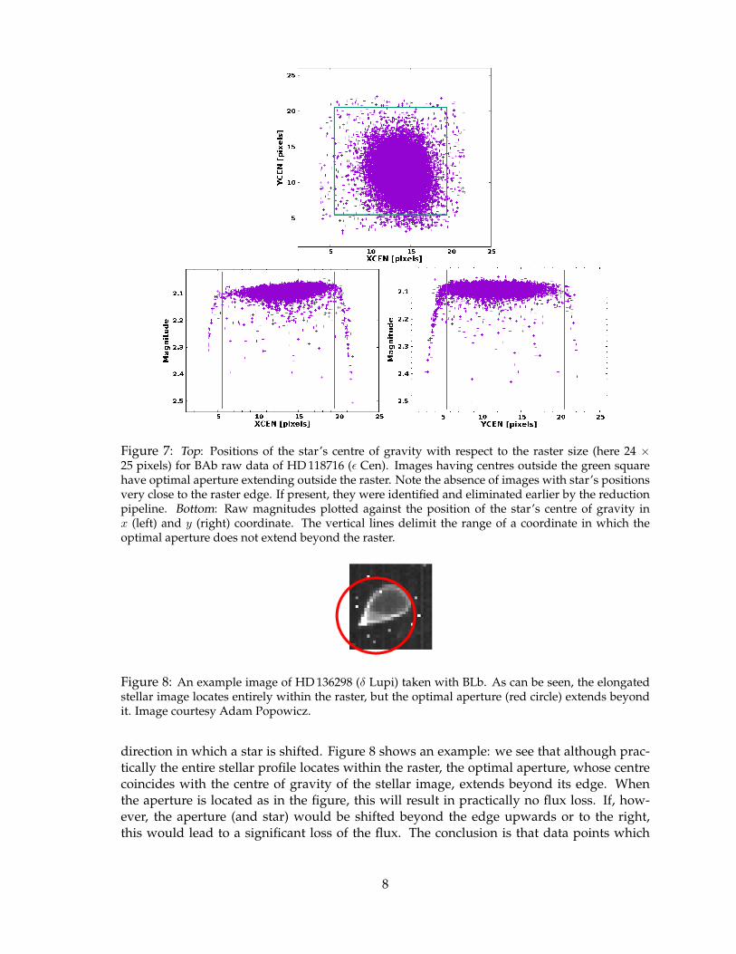
Figure 7: Top: Positions of the star’s centre of gravity with respect to the raster size (here 24 ×25 pixels) for BAb raw data of HD 118716 (ε Cen). Images having centres outside the green squarehave optimal aperture extending outside the raster. Note the absence of images with star’s positionsvery close to the raster edge. If present, they were identified and eliminated earlier by the reductionpipeline. Bottom: Raw magnitudes plotted against the position of the star’s centre of gravity inx (left) and y (right) coordinate. The vertical lines delimit the range of a coordinate in which theoptimal aperture does not extend beyond the raster.

Figure 8: An example image of HD 136298 (δ Lupi) taken with BLb. As can be seen, the elongatedstellar image locates entirely within the raster, but the optimal aperture (red circle) extends beyondit. Image courtesy Adam Popowicz.

direction in which a star is shifted. Figure 8 shows an example: we see that although prac-tically the entire stellar profile locates within the raster, the optimal aperture, whose centrecoincides with the centre of gravity of the stellar image, extends beyond its edge. Whenthe aperture is located as in the figure, this will result in practically no flux loss. If, how-ever, the aperture (and star) would be shifted beyond the edge upwards or to the right,this would lead to a significant loss of the flux. The conclusion is that data points which

8

are now regarded as outliers because the optimal aperture extends beyond the raster edgecome from images that can still be useful provided that appropriate changes to the pipelinewill be applied. For the current data release, however, there is no simple way to distinguishthem. In the future reductions and data releases it is planned to use non-circular apertureswith shapes adjusted to stellar profiles. This would solve the problem. For the current datarelease you may consider using some points flagged with ‘0’ using a different range of al-lowable positions. In such a case, however, it is the best to plots similar to those in Fig. 7,bottom panels.

Having removed the outliers due to aperture extending beyond the raster, we are leftwith the light curve which is shown in Fig. 9. As one can see, there is still a lot of outliers left.Their origin is different. An inspection of the corresponding images shows that they occurdue to the factor (B) discussed above (Sect. 2), i.e. a motion of a star during an exposure. Sucha motion smears stellar images. Since a constant circular aperture is used, a consequence ofsuch smearing is again a loss of a part of the flux. This is rather bad news because there is noeasy way to improve it. In addition, due to this effect we cannot expect a normal distributionof data points in an orbital sample. It is, however, sensible to remove these outliers too. Weexplain below how this can be done.

Figure 9: The light curve of HD 118716 (ε Cen) in the Centaurus field, the same as shown in Fig. 6,after removing the points flagged as outliers. For a better comparison, the magnitude range is thesame as in Fig. 6.

In Sect. 2 we mentioned that in addition to the motion of stars there is another factor,(C), that blurs images: the occurrence of CTIs. CTIs also lead to a flux loss. Since CTI isa permanent defect, its effect on a light curve would not be the occurrence of outliers butrather a sudden drop of the flux level. An example of the effect of the occurrence of the CTIis shown in Fig. 10. This kind of behaviour allows for an easy identification of the occurrenceof a CTI and removal of affected data points.

As one can judge from Figs 9 and 10, outlier removal is not always a necessary step whenworking with BRITE data. While it should be applied to the data shown in Fig. 9, the ‘pre-CTI’ part of the BTr data for HD 191610 (Fig. 10) is almost free of outliers. In general, outlierremoval has to be applied to all BAb and UBr data, while for the other satellites it should bedecided on a star by star basis.16

When outlier removal is a must, how can it be done in a robust way? Well, again, thereis no single, best way to remove outliers. There are many methods that can be used for thispurpose, e.g. sigma(σ) clipping. One thing I would like to suggest is to work with orbit sam-ples when doing outlier removal. The orbits typically contain enough data points to safely

16As one can guess, this is a consequence of the differences in the quality of tracking, see also Sect. 5.2.1.

9

Figure 10: An example of the influence of the occurrence of the CTI for the BTr photometry ofHD 191610 (28 Cyg): a sudden drop in magnitude after HJD 2456878.

remove outliers on a statistical basis. Next, as I will show later, the scatter in consecutiveorbits may differ a lot. Working with samples larger than a single orbit would definitelypose problems. This would, for example, require removal of intrinsic variability prior todetecting outliers.

An important question arises at this point: should we remove intrinsic variability priorto the outlier removal or not? I would say: it depends. If (i) the time scale of variability isconsiderably longer than the length of a single orbit observation, or (ii) the amplitudes aremuch smaller than scatter of points within a single orbit, you do not need to bother aboutremoving the intrinsic variability (at least at this step). What if one needs to or simply wantsto do this anyway? A simple recipe can be the following:

1. Remove outliers in a simple way, e.g. preserving only those points which fall in acertain range of magnitudes/fluxes. This will not remove all outliers but those thatdeviate most will be removed. For example, for data shown in Fig. 9, one can removeall data points that have magnitudes larger than 2.16. This can be done e.g. by putting:> awk ’{if ($2<2.16) print $0}’ lc.data > lc.tmp; mv lc.tmp lc.data

2. Calculate periodogram(s), identify intrinsic frequencies and subtract them from theoriginal data.17 Then, you have to work with residuals.

One can also consider to apply outlier removal not just once but several times, e.g. againafter decorrelating the data (see the next subsection). In such a case, one can start with amild removal criterion, strengthening it in further steps.

Let us go over the methods. I have implemented the GESD algorithm,18 which is claimedto be quite robust. Details of the algorithm can be found in the web page quoted in the foot-note. One can, of course, use any other algorithm, e.g. σ-clipping which should also workwell. In order to support those who want to use the GESD algorithm, I provide a Fortranprogram outl-gesd.f. In my computer, I use gfortran to compile it, but I suppose it canbe used with other compilers as well. The program has to be run with a single parameter19,a level of significance α, α > 0:

17This can be efficient only when dealing with periodic variability that can be well approximated with a seriesof sinusoids.

18GESD stands for Generalized Extreme Studentized Deviate. The description of the algorithm canbe found at http://www.itl.nist.gov/div898/handbook/eda/section3/eda35h3.htm. It is implemented e.g.in Matlab (http://www.mathworks.com/matlabcentral/fileexchange/28501-tests-to-identify-outliers-in-data-series/content/gesd.m), but one can look for it in other packages as well.

19A more detailed description of this and the other provided programs is given in the Appendix (Section 8).

10

> ./outl-gesd [alpha]

The larger α, the more outliers are detected. How to choose this parameter optimally20?The answer is not obvious and can be different for different data sets. If one works withnormally distributed samples, one could use a typical value, e.g. 0.05 or 0.1. This can bethe case for BTr data. For satellites with a larger number of outliers, I would suggest usinglarger α (formulation of the algorithm allows one to adopt even α > 1).

Figure 11: Fraction of detected outliers (in %) as a function of α for BAb data of HD 118716.

I have made some tests using the BAb and UBr data for α Cir. In general, stronger outlierremoval results in smaller scatter but also in a smaller number of data points that are left.Consequently, the detection threshold in the periodogram, D, which depends both on thenumber of data points (the fewer the points, the higher is D) and the scatter (the smaller thescatter, the lower is D), can reach a minimum for a certain α. Should we use a minimumin the D(α) relation to choose optimal α? Well, rather no. Why? It happens that there isno distinct minimum in D(α) at all or the minimum occurs for large α corresponding to avery large number of outliers removed. I would therefore suggest not to use the minimumof D(α) for choosing α. Before more tests will be done and some general conclusion drawn,it is better to try several values of α and then adopt the preferred value based on the resultsit produces. As an example, I show in Fig. 11 the fraction of detected outliers (in percent) inthe full data set plotted as a function of α. This is done for the data set shown in Fig. 9. Thesaturation at 30% is a result of setting the upper limit for the fraction of outliers in the GESDalgorithm (here set at 30% of the original sample). The result of outlier detection is shown inFig. 12. As can be seen, there are points that passed outlier detection although they clearlydeviate from the mean. These are simply orbits with higher scatter. They will be eliminatedlater; see Section 5.2.2.

5.2 Decorrelations

Having removed outliers, one can perform the next step in the analysis, decorrelation. Theraw BRITE magnitudes correlate (sometimes strongly) with temperature, position of thecentroid, orbital phase and maybe other, yet not discovered factors. Decorrelation is, in myopinion, a necessary step in the analysis of BRITE data because it can significantly improvethe photometry. It would be the best to make multi-dimensional decorrelation in one step.However, the correlations, as I will show later, cannot be described with a simple function

20α is the level of significance, but since the distribution of points for a single orbit is far from normal, αshould be treated rather as a free parameter not a statistical parameter with the common meaning.

11

Figure 12: Result of outlier removal for data shown in Fig. 9 with the GESD algorithm and α = 0.3.Red points are those which passed outlier detection, blue ones, detected outliers.

and therefore I do decorrelations step by step. You are welcome to do this in your own way.Yes, there is no single best way to decorrelate BRITE data.

Figure 13: Chip temperature as a function of time for reduced BRITE data. Different colours areused for different satellites: dark blue: BAb, light blue: BLb, red: UBr, orange: BTr.

5.2.1 What to expect?

Why do correlations occur? Let us start with chip temperature, T , given in the fifth columnof the BRITE data files (Fig. 4). In most ground-based systems, CCDs are cooled and thetemperature is stabilized. There is no cooling onboard BRITEs, so that chip temperaturereflects thermal response of the whole satellite for illumination by the Sun. I can easilyimagine that the variable temperature of a BRITE CCD chip and whole electronics leads tothe occurrence of a temperature effect. Figure 13 shows how temperature changes with timefor four satellites during the observations of the first four fields (Ori, Cen, Sgr, Cyg). Thecharacter of these changes depends mainly on the satellite’s orbit and orientation. Note thatthere is a change of temperature within a single orbit (its range corresponds to the verticalwidth of a strip). A close-up shows that during observations made within a single orbit, thetemperature usually increases.

That magnitudes in BRITE photometry depend on centroid position, xcen and ycen (thirdand fourth column in data file), is not a surprise. The factor (B) mentioned in Sect. 2 leadsnot only to the additional smearing of stellar profiles but also to wandering of a star within

12

Figure 14: Positions of stellar centres of gravity, xcen (top) and ycen (bottom) for the same data andcolour coding as in Fig. 13. The positions are plotted for: ψ2 Ori in Ori field, ε Cen in Cen field, κ Scoin Sgr field, and ε Cyg and σ Cyg in Cyg field.

a raster. Therefore, despite the attempts to aim a satellite in the same direction on differentorbits, the positions of a star are different for different orbits. This can be seen in Fig. 14where xcen and ycen are shown as a function of time. In the lack of flat-fielding as is the casefor the BRITEs, a dependence of the measured flux on position is something which can beexpected. In consequence, the better the stability of a position, the better the photometry. Ascan be seen in Fig. 14, BTr and BLb are better stabilized than BAb and UBr. As mentionedby Weiss et al. (2014, Sect. 6.1), BTr and BLb have better trackers than BAb and UBr. As aconsequence, the BLb and BTr photometry can be expected to show smaller scatter than BAband UBr.21 This is indeed what we see.

In addition to the dependence on T , xcen and ycen, one can expect to see instrumentaleffects related to orbital phase. It seems that for BRITEs this is a rather complicated depen-dence which causes not only an occurrence of a single peak at the orbital frequency (and itsharmonics), but rather a bunch of peaks close to the orbital frequency (and its harmonics).One can therefore apply decorrelation with orbital phase. This will lower the amplitudeof the orbital frequency and its harmonics, but it cannot be expected that all orbit-relatedinstrumental signals will be removed in this way.

In order to be able to remove the dependence on orbital phase, we need to have the or-

21Since BAb and UBr are longer in space than the other BRITEs, they are also exposed longer to radiation dam-age effects. This is another reason for poorer photometry from these satellites when compared to simultaneousobservations from other BRITEs.

13

bital phase as an additional column in our working file. For this purpose, I provide anotherFortran program phase-B.f. Its syntax is the following:> ./phase-B [inp file] [init epoch] [period] [outp file]

The program reads inp file, calculates orbital phases and adds sixth column with phases.The result is stored in file outp file. A sample record in our working file lc.data looksnow like this:

756.5911658 2.1034428 12.71 14.89 34.18 0.647909

The orbital periods (in minutes) are given in Table 1. Note, however, that the satellite orbitalperiods are not constant. The periods given in Table 1 are temporary values. The true valueof the period is not very much different, but should be derived from the frequency spectrum.For example, the BAb data for ε Cen were phased with the period of 100.418 minutes.

5.2.2 Two preliminary steps

There are still two steps that need to be done before we start decorrelations: (i) removalof the worst (in the sense of the highest scatter) orbits and (ii) subtraction of any strongintrinsic signal. Step (i) needs to be done because the worst orbits sometimes have meanmagnitudes that differ significantly from the rest (see Fig. 15 below) and this would affect thecorrelations. For the same reason, step (ii) is necessary if the intrinsic variations have largeamplitudes. Note that you do not need to make a complete solution at this step: it is enoughif you remove only the strongest variability. Although I would recommend doing (i) before(ii), a reversed sequence is allowable, too. Finally, an important note on intrinsic variability:if (multi)periodic, it can be easily subtracted. If not, we can have a problem, especially whenthe time scale of variability is comparable to the time scale of the variability of T or anyother parameter. In such a case, it might not be possible to unambiguously separate intrinsicvariability and instrumental effects due to correlation with some parameter (especially T ).In other words, removing correlations can also partly remove long-term intrinsic variability.

Let us have a look at an example of step (i). Figure 15 (top) shows standard deviationsfor orbit samples for the same data as shown in Fig. 12 (BAb observations of ε Cen). Onecan see that removing orbits that have the highest standard deviations removes also most ofthose points that deviate from the mean (bottom panel). Obviously, this procedure wouldnot remove deviating points which are due to intrinsic variability (e.g. short eclipses) —which is good.

In order to support those who do not want to write their own software, I provide theprogram orbits.f, which calculates standard deviations for orbit samples. It has twoparameters, the name of a file with light curve and the name of a file with residuals. If youdid not subtract intrinsic variability before this step (i.e. you do not have residuals yet), usethe name of a file with the light curve for both parameters. Assuming that our working filewith the light curve is named lc.data and the file with residuals is named resid.data,you can run the program like this:> ./orbits lc.data resid.data

or, if you do not have residuals:> ./orbits lc.data lc.data

One of the output files is file lc.data.sig which has seven columns. The extra column(inserted as the third one) is the standard deviation, σ, calculated separately for each orbit.The σs can be used as uncertainty needed in some fitting programs.

14

Figure 15: Top: Standard deviations for orbit samples for BAb data of ε Cen. Encircled pointsindicate orbits that are rejected due to their high scatter. Bottom: The result of rejection of the worstorbits. Data points from removed orbits are shown in blue.

Now for step (ii), i.e. subtraction of intrinsic variability. For our example star, the β Ce-phei-type star ε Cen, I have subtracted the three strongest modes with frequencies 5.896,6.183 and 5.689 d−1 and stored the residuals in file resid.data. You can use any soft-ware to fit and subtract periodic variability. It is, however, important to have two files: thefile with the light curve and the file with residuals (for simplicity named here lc.dataand resid.data, respectively). I will assume that they have the same format, i.e. containseven columns: (1) time, (2) magnitude, (3) uncertainty of (2), (4) xcen, (5) ycen, (6) T , (7) or-bital phase. Note that lc.data and resid.data should contain the same number of datapoints and have the same entries in all columns but the second. From this point on we willwork with resid.data to calculate correlations, but the corrections to light curve due tocorrelations will be applied to lc.data.

5.2.3 How to decorrelate?

Since we have four parameters to check correlations of magnitudes with (xcen, ycen, T andorbital phase, φ), we have to decide on the sequence in which we do that. Depending on thesequence we choose, the result will be different. Based on some tests I made, the expectedconclusion is that it is best to start with the strongest correlation and then proceed with suc-cessively weaker ones. Usually the correlation between magnitudes and T is the strongest,but this also depends on the star. The temperature effect can be seen for all satellites but isusually most pronounced for BAb data. Figure 16 shows the correlations between residualmagnitudes and the four considered parameters for BAb data of ε Cen. At least for this data

15

Figure 16: Correlations between residual magnitude and four considered parameters for BAb dataof εCen. The black circles are the anchor points calculated in parameter intervals (two extreme pointsare linearly extrapolated). The continuous line is the interpolated (by means of Akima interpolation)relation that uses anchor points.

set the correlations are not strong and the largest effect can be seen for xcen. The sequence ofdecorrelation was therefore the following in this case: xcen — T — ycen — φ.

We get a very different picture of the correlations for the BAb data of another star, α Cir(Fig. 17). This time the correlation with temperature is very strong and reaches a range of0.2 mag. The decorrelation sequence was different in this case: T — xcen — ycen — φ.

In order to support this step of analysis, I provide another Fortran program, decor.f.Its syntax is the following:> ./decor [lc.data] [resid.data] [N aver] [N c],where file names lc.data and resid.data stand for two files whose contents were ex-plained above (you can, of course, use other names), N aver is the number of anchor pointsfor averages calculated for a given parameter (plotted as black circles in Figs 16 and 17) andN c is the sequential number of a column with a parameter with which we calculate thecorrelation. As a reminder: the 4th column of lc.data and resid.data contains xcen,5th, ycen, 6th, T , and 7th, φ. The program works on residuals (file resid.data). It sorts

16

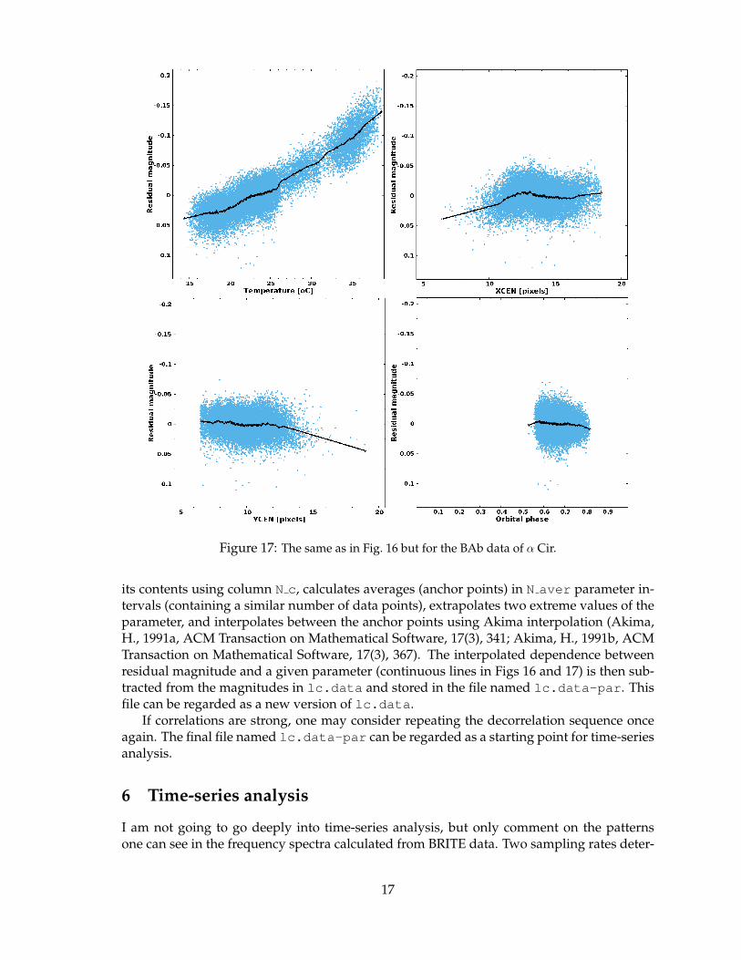
Figure 17: The same as in Fig. 16 but for the BAb data of α Cir.

its contents using column N c, calculates averages (anchor points) in N aver parameter in-tervals (containing a similar number of data points), extrapolates two extreme values of theparameter, and interpolates between the anchor points using Akima interpolation (Akima,H., 1991a, ACM Transaction on Mathematical Software, 17(3), 341; Akima, H., 1991b, ACMTransaction on Mathematical Software, 17(3), 367). The interpolated dependence betweenresidual magnitude and a given parameter (continuous lines in Figs 16 and 17) is then sub-tracted from the magnitudes in lc.data and stored in the file named lc.data-par. Thisfile can be regarded as a new version of lc.data.

If correlations are strong, one may consider repeating the decorrelation sequence onceagain. The final file named lc.data-par can be regarded as a starting point for time-seriesanalysis.

6 Time-series analysis

I am not going to go deeply into time-series analysis, but only comment on the patternsone can see in the frequency spectra calculated from BRITE data. Two sampling rates deter-

17

mine the alias pattern of the data. The first one is related to consecutive images which aretypically 1-second exposures separated by 20–23 seconds. This means that the Nyquist fre-quency related to this sampling is very high (∼2000 d−1) and very high frequencies22 can, inprinciple, be detected in the data. The problem is that there are very few stars among thosethat BRITE can properly observe in which such high frequencies are expected. The rapidlyoscillating Ap star α Cir with its 210 d−1 pulsation is probably one of very few. The othersampling rate is related to the BRITE orbital period which amounts to about 100 minutes(see Table 1) corresponding to orbital frequency forb ≈ 14.4 d−1. The resulting Nyquist fre-quency fN,orb = forb/2 ≈ 7.2 d−1 is in the range of frequencies typical for β Cep and δ Sctstars. Let us have a look at the frequency spectrum of the data we used as an example, i.e.,BAb data of the β Cephei-type variable ε Cen.

Figure 18: Top: Frequency spectrum of BAb data of ε Cen in the range 0–250 d−1. Bottom: The sameas above but in the range of 0–25 d−1. Two arrows indicate frequencies discussed in the text, forb andfN,orb = forb/2.

Figure 18 shows the frequency spectrum of BAb data for this star in two different ranges:up to 250 d−1 and up to 25 d−1. The three high peaks between 5 and 7 d−1 ( 5.896, 6.183 and5.689 d−1) are the three strongest pulsation modes. The aliases of these frequencies occur atfrequencies nforb+fi and nforb−fi, where n is an integer number and fi is the frequency ofan intrinsic variation. The aliases can be seen even at very high frequencies. The envelope ofthe peaks is simply an absolute value of the sinc (sinx/x) function related to the width of theobservations made during a single orbit (about 12.5 minutes). It is obvious that high aliasesmay pose a problem with ambiguous identification of intrinsic variability if frequencies areclose to fN,orb. We will now show that it really is the case.

Having prewhitened the three strongest modes, we get a frequency spectrum which isshown in Fig. 19. At low frequencies, we get three peaks corresponding to the combinationfrequency (6.183 − 5.896 = 0.287 d−1) and two other close frequencies, presumably g modes.

22Because exposures are much shorter than the sampling interval, frequencies much higher than the Nyquistfrequency can be detected without a significant reduction of amplitude.

18

Figure 19: Frequency spectrum of BAb data of ε Cen after prewhitening with the three strongestmodes.

At higher frequencies we get two pairs23 of significant peaks (corresponding to the next twomodes), one pair at 6.318 and 8.023 d−1 and the other at 4.485 and 9.855 d−1. We thereforeface a problem of ambiguous identification of intrinsic frequencies. As I will show below,this problem can be solved by combining data from all satellites, even with mixed blue andred filters. In addition, peaks around 1 and 2 d−1 can be seen in some frequency spectra (e.g.,in Fig. 19). The occurrence of these peaks seems to be a surprise for satellite data, but sincethe satellites are in low orbits, Earth rotation-related instrumental effects can be present.

6.1 The power of combining

Finally, I would like to recommend combining the data from different satellites even ifthey were not obtained with the same filter. There are two main advantages of combiningthis way: (i) lowering of the detection threshold, which may allow for detection of low-amplitude modes, (ii) lowering of aliases (because the orbits and orbital periods of BRITEsare different, the data from one satellite fill gaps in the observations of the other, see Fig. 20)which helps to identify unambiguously the true frequencies. Warning: if amplitudes in thered and blue filters differ considerably, a residual signal close to prewhitened frequenciescan occur. In such a case you may try to scale one filter data with the amplitude ratio priorcombining.

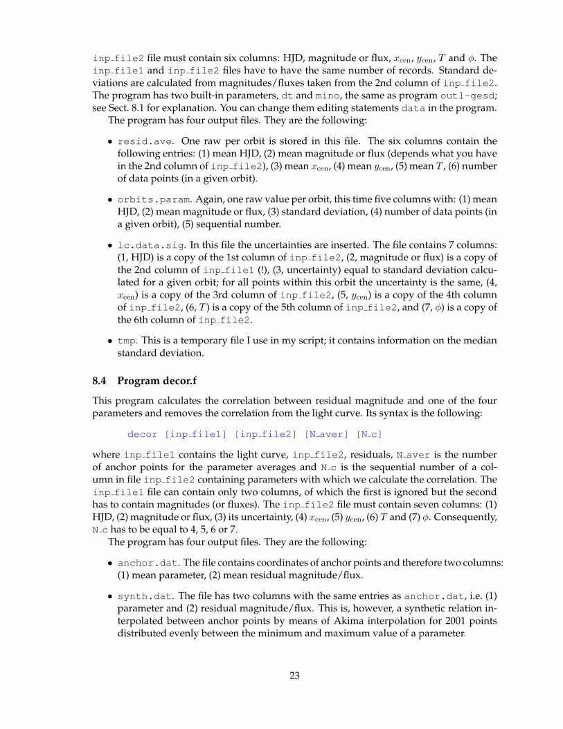
Let us see what we get if we combine data from all four satellites (BAb, BLb, UBr andBTr) for ε Cen. Of course, prior to combining, the user has to account for the differencesin mean magnitudes. Comparing the frequency spectrum of the combined data (Fig. 21)with that of BAb data (Fig. 18), we see that the aliases in the spectrum of the combined dataare much lower. As a consequence, the problem illustrated in Fig. 19 is now solved: of thetwo possibilities for two pairs of peaks discussed above, it is clear that the true frequenciesare 4.485 and 6.318 d−1. Many more modes can also be seen above the noise level. Thus,this is also a good example of advantage (i). A detailed analysis of blue-filter data reveals 9significant modes: 7 p, 2 g plus one combination. A similar analysis of red-filter data gives10 modes: 8 p, 2 g and the same combination. Finally, analysis of the combined data yieldsfrequencies of 13 modes (9 p and 4 g) plus one combination frequency. Only 5 of them areknown from the literature. I hope this shows that new science can be made with BRITE dataand that combining quasi-simultaneous data from different satellites is worth doing.

At a higher frequency range (13 – 16 d−1) we can see the orbital frequency and its dailyaliases.

23A pair consists of a frequency of intrinsic variability and its alias mirrored with respect to fN,orb.

19

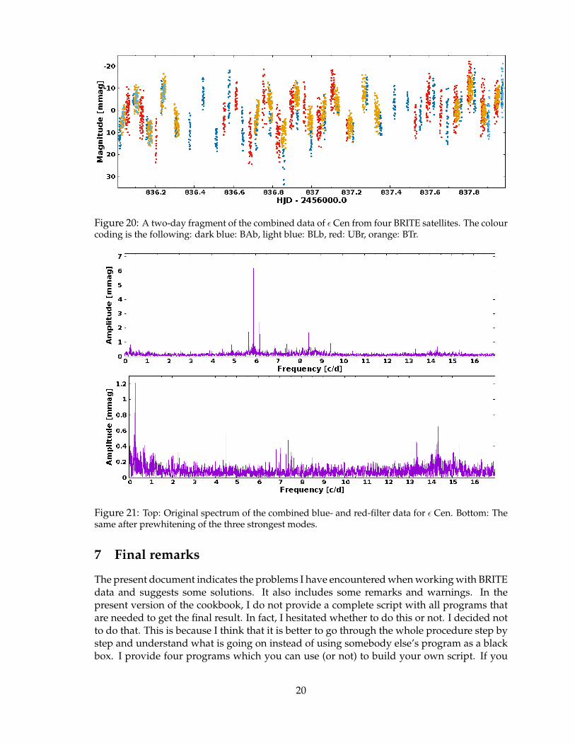
Figure 20: A two-day fragment of the combined data of ε Cen from four BRITE satellites. The colourcoding is the following: dark blue: BAb, light blue: BLb, red: UBr, orange: BTr.

Figure 21: Top: Original spectrum of the combined blue- and red-filter data for ε Cen. Bottom: Thesame after prewhitening of the three strongest modes.

7 Final remarks

The present document indicates the problems I have encountered when working with BRITEdata and suggests some solutions. It also includes some remarks and warnings. In thepresent version of the cookbook, I do not provide a complete script with all programs thatare needed to get the final result. In fact, I hesitated whether to do this or not. I decided notto do that. This is because I think that it is better to go through the whole procedure step bystep and understand what is going on instead of using somebody else’s program as a blackbox. I provide four programs which you can use (or not) to build your own script. If you

20

need anything else that would help you in the analysis and is lacking here, please let meknow.

Finally, I would like to ask you to contribute to this document with your knowledge andexperience gained from the work with BRITE data. And above all ... have fun!

Acknowledgements. I would like to thank very much to all those (especially the membersof the PHOTT) who contributed to this document with all ideas and insights expressedin many discussions: Gerald Handler, Rainer Kuschnig, Tony Moffat, Bert Pablo, AdamPopowicz, Tahina Ramiaramanantsoa, Jason Rowe, Sławek Rucinski, Gemma Whittaker,Werner Weiss, and Ela Zocłonska. Special thanks to Tony Moffat for corrections made uponreading the draft of the document.

21

8 Appendix

8.1 Program outl-gesd.f

The program identifies outliers. Its syntax is the following:

outl-gesd [alpha]

where alpha is the level of significance, α; α has to be larger than 10−8. The program hassome built-in parameters. You can change them editing the program. These are:

• maximum length of data during a single orbit, dt. The parameter is used to separatedata points made during different orbits. It is now set to 50 minutes (half an orbitalperiod). If longer observations per orbit are expected, you can change it (see statementdata at the beginning of the program).

• maximum number of outliers (in per cent of the original sample), pmax. This param-eter limits the number of outliers to be identified. Regardless of the value of α, thenumber of outliers in a sample will not exceed pmax. The parameter is presently set to30 (per cent).

• minimum number of exposures per orbit, mino. If only mino or fewer data points areleft in an orbit sample, the whole orbit is flagged as outliers.

It is assumed that the input file is named lc.data. It should have at least 5 columns sepa-rated by spaces/tabs: HJD, magnitude or flux, xcen, ycen, T . The other columns, if present,are ignored. Two output files are created: lc.ror which contains 5 columns copied fromlc.data and a sixth column which contains either 0 (a data point is not an outlier) or 1 (out-lier). The column can be subsequently used to make a file free of outliers, e.g. by putting:> awk ’{if ($6 == 0) print $0}’ lc.ror > lc.tmp

8.2 Program phase-B.f

The program calculates orbital phases. Its syntax is the following:

phase-B [inp file] [init epoch] [period] [outp file]

where inp file is the input file, usually lc.data, init epoch is the initial epoch (canbe set any value), period is the orbital period of a satellite, and outp file is the outputfile. It is assumed that inp file has five columns. They are copied to outp file; the sixthcolumn which is added by the program to outp file contains orbital phases, φ, 0 ≤ φ < 1.

8.3 Program orbits.f

The program calculates standard deviations using individual orbits and adds them as un-certainties to the light curve. Its syntax is the following:

orbits [inp file1] [inp file2]

where inp file1 is a file with a light curve and inp file2 is a file with residuals. If theuser has not subtracted any intrinsic variability and has no file with residuals, inp file2can be the same as inp file1. In principle, inp file1 can contain only two columns,of which the first is ignored but the second has to contain magnitudes or fluxes. The

22

inp file2 file must contain six columns: HJD, magnitude or flux, xcen, ycen, T and φ. Theinp file1 and inp file2 files have to have the same number of records. Standard de-viations are calculated from magnitudes/fluxes taken from the 2nd column of inp file2.The program has two built-in parameters, dt and mino, the same as program outl-gesd;see Sect. 8.1 for explanation. You can change them editing statements data in the program.

The program has four output files. They are the following:

• resid.ave. One raw per orbit is stored in this file. The six columns contain thefollowing entries: (1) mean HJD, (2) mean magnitude or flux (depends what you havein the 2nd column of inp file2), (3) mean xcen, (4) mean ycen, (5) mean T , (6) numberof data points (in a given orbit).

• orbits.param. Again, one raw value per orbit, this time five columns with: (1) meanHJD, (2) mean magnitude or flux, (3) standard deviation, (4) number of data points (ina given orbit), (5) sequential number.

• lc.data.sig. In this file the uncertainties are inserted. The file contains 7 columns:(1, HJD) is a copy of the 1st column of inp file2, (2, magnitude or flux) is a copy ofthe 2nd column of inp file1 (!), (3, uncertainty) equal to standard deviation calcu-lated for a given orbit; for all points within this orbit the uncertainty is the same, (4,xcen) is a copy of the 3rd column of inp file2, (5, ycen) is a copy of the 4th columnof inp file2, (6, T ) is a copy of the 5th column of inp file2, and (7, φ) is a copy ofthe 6th column of inp file2.

• tmp. This is a temporary file I use in my script; it contains information on the medianstandard deviation.

8.4 Program decor.f

This program calculates the correlation between residual magnitude and one of the fourparameters and removes the correlation from the light curve. Its syntax is the following:

decor [inp file1] [inp file2] [N aver] [N c]

where inp file1 contains the light curve, inp file2, residuals, N aver is the numberof anchor points for the parameter averages and N c is the sequential number of a col-umn in file inp file2 containing parameters with which we calculate the correlation. Theinp file1 file can contain only two columns, of which the first is ignored but the secondhas to contain magnitudes (or fluxes). The inp file2 file must contain seven columns: (1)HJD, (2) magnitude or flux, (3) its uncertainty, (4) xcen, (5) ycen, (6) T and (7) φ. Consequently,N c has to be equal to 4, 5, 6 or 7.

The program has four output files. They are the following:

• anchor.dat. The file contains coordinates of anchor points and therefore two columns:(1) mean parameter, (2) mean residual magnitude/flux.

• synth.dat. The file has two columns with the same entries as anchor.dat, i.e. (1)parameter and (2) residual magnitude/flux. This is, however, a synthetic relation in-terpolated between anchor points by means of Akima interpolation for 2001 pointsdistributed evenly between the minimum and maximum value of a parameter.

23

• resid.dat-par and lc.data-par. These two files contain seven columns withthe same entries as inp file2. All columns but the second are copied to these filesfrom inp file2. The only difference is the second column. In this column in filelc.data-par the light curve (2nd column of inp file1) corrected for the derivedcorrelation is stored. Similarly, in the second column of file resid.dat-par the resid-ual light curve (2nd column of inp file2) corrected for the derived correlation isstored.

24