Automation, Vol. 26, No. 4, pp. 721-737, 1990 Print¢d in Great Britain.

0005-1098/90 $3.00 + 0.00 Pergamon Press pie

(~) 1990 International Federation of Automatic Control

Analysis and Simulation of Strong Earthquake Ground Motions Using ARMA Models*

TH. D. P O P E S C U t and S. DEMETRIUS:

Segmentation of the nonstationary time series and representation of the quasi-stationary data blocks through ARMA models provides an efficient and flexible procedure for characterization of earthquake ground motions.

Key Words--Time-series analysis; signal processing; parameter estimation; simulation; ARMA models; nonstationarity analysis; geophysics; earthquake ground motion.

Abstract--The acceleration record of an earthquake ground motion is a nonstationary process with both amplitude and frequency content varying in time. The paper presents a general procedure for the analysis and simulation of strong earthquake ground motions based on parametric ARMA models to be used in computing structural response. Some computational results obtained in the analysis and simulation of ground acceleration, recorded during the Romanian Earthquake of 4 March 1977, are also included.

1. INTRODUCTION IT HAS aECOME relatively common practice in recent years to use stochastic processes as models of dynamic loadings that are subject to considerable uncertainty, such as earthquake ground motion, or forces caused by wind or waves. The particular problem considered in this paper is the analysis and simulation of ear thquake ground motions, although the results may be also applicable to other similar problems.

The analysis and simulation of strong ear thquake ground motions may prove very useful, especially for the design of complex structures that are expected to have nonlinear behaviour during seismic motion, allowing a statistical treatment of the response characteris-

* Received 25 October 1988; revised 29 March 1989; received in final form 4 October 1989. The original version of this paper was presented at the 8th IFAC/IFORS Symposium on Identification and System Parameter Estima- tion which was held in Beijing, People's Republic of China during August 1988. The Published Proceedings of this IFAC Meeting may be ordered from: Pergamon Press pie, Headington Hill Hall, Oxford OX3 0BW, U.K. This paper was recommended for publication in revised form by Associate Editor Y. Sunahara under the direction of Editor P. C. Parks.

"I" Institute for Computers and lnformatics 8-10 Miciurin Bird, 71316 Bucharest, Romania.

¢ Faculty of Civil Engineering 124 Lacul Tei Blvd, 72302 Bucharest, Romania.

721

tics. The analysis and simulation problems of seismic signals can be stated as follows:

(a) Analysis problem: to develop a method of nonstationary characterization of earthquake accelerograms that can describe the time-varying nature of the mean square amplitude and spectral content.

(b) Simulation problem: to recover the original accelerogram or a class of compatible time functions, given the solution for (a).

Historically, the modelling and application of nonstationary covariance time series in en- gineering applications have been approached via the fitting of locally stationary models, via orthogonal polynomial expansion of AR coefficient models, and other analyses of random coefficient A R models. Locally, stationary AR modelling was shown by Ozaki and Tong (1975) and Kitagawa and Akaike (1978),

The analysis and simulation of nonstationary processes have been studied mostly in connec- tion with ear thquake ground motions. The common feature of these studies is that a nonstationary process can be simulated by multiplying by an envelope function of a stationary process generated either by filtering a white noise (Jennings et al., 1968), or by a series of waves with random frequency and random phase (Kitada et al., 1983). Some relatively new methods employ the class of autoregressive models (AR) (Kozin, 1979; Jurkevics and Ulrich, 1978; Gersh and Kitagawa, 1985) and the general class of autoregressive moving average (ARMA) models for the analysis and simulation of strong motion accelerations (Nau et al., 1980). Kozin (1979) shows an orthogonal polynomial expansion of the A R coefficients of a time- varying A R model. The method is extended by Gersh and Kitagawa (1983) to a multivariate time-varying A R model in the context of

722 TH. D. PoPESCU and S. DEMETRIU

econometric data analysis. Jurkevics and Ulrich (1978) use an "adaptive filtering" method for estimating time-varying parameters in an AR model. The similarities and differences between adaptive filtering methods and Kalman filtering methods for estimating time-varying AR para- meters have been discussed in a paper by Nau and Oliver (1979). In Gersh and Kitagawa (1985), the nonstationary time series is modelled by a time-varying autoregressive (AR) model with smoothness constraints on the time-evolving AR coefficients. The analysis yields the sequence of instantaneous time-varying AR coefficients and the process variance and may have numerous engineering applications. The major contribu- tions of the report elaborated by Nau et al. (1980) are the use of Kalman filters for estimating time-varying A R M A model para- meters, and the development of an effective non-parametric method for estimating the variance envelopes of the accelerogram records.

The AR and ARMA models represent filters used for the generation of the synthetic accelerograms by passing an approximation of a white noise through them. Also, the evaluation of ARMA and related parameters, on their own, has physical significance for certain model structures and is related to parameters such as earthquake intensity and duration, distance to the fault and local geology (Cakmak and Sheriff, 1984).

In particular, the application of ARMA models to strong motion accelerograms can be performed after processing the seismic signals by a variance stabilizing transformation (Polhemus and Cakmak, 1981).

In the present paper the problem of signal nonstationarity is solved by segmenting the original data, using the evaluation of Akaike Information Criterion (AIC) for different data blocks (Kitagawa and Akaike, 1978), so that each data block could be considered quasi- stationary. For each quasi-stationary data block an ARMA model is fitted by canonical correlation analysis and exact maximum like- lihood method. These models are used for simulation purposes, to recover the original seismic signal. Finally, the original and synthetic data, obtained from ARMA models in a case study, are compared by evaluating a number of statistical characteristics and parameters, com- monly used to characterize strong motion accelerograms. An acceptance match is found in all cases. The application of the time domain technique for the analysis and simulation of digitized earthquake accelerograms, presented in the paper, seems to be a potentially useful method of characterizing earthquake ground

motions by constant linear models with a small number of parameters.

2. M O D E L L I N G OF NONSTATIONARY TIME SERIES

Nonstationarity analysis In certain situations the statistical characteris-

tics of a natural time series are a function of time. To model an observed time series that possesses nonstationarity, a common procedure is to first remove the nonstationarity by invoking a suitable transformation and then to fit a stationary stochastic model to a transformed sequence. When modelling certain types of geophysical time series, it is often reasonable to assume that the time series are approximately stationary over a specified time interval. The problem of signal nonstationarity is solved in this paper by segmenting the original data, so that each data block can be considered quasi- stationary.

The nonstationarity analysis procedure used (Kitagawa and Akaike, 1978), originally pro- posed by Ozaki and Tong (1975), is suitable for application to a nonstationary situation where the analysis of a short span of data is necessary. The procedure is discussed in detail in Kitagawa and Akaike (1978). Here we will give only a conceptual description of the procedure.

Suppose we have a set of initial data Y~,Y2 . . . . . Yr., and an additional set of S observations YL+I . . . . . YL+S is newly obtained, where S is a prescribed number. The procedure is as follows:

(1) Fit an autoregressive model ARo, y, =

A,,,y~_,,, + e , , with tr 2 the innovation vari- m=l

ance, where Mo is chosen as the one which gives the minimum of the criterion AIC, for the set of data y~, Y2 . . . . , yL.

AICo = L- log ~o + 2(Mo + 2). (1)

(2) Fit an autoregressive model AR1, Yn = M1 E A,,,yn-,~ + en, with 02 the innovation vari-

m=l

ance, and Mt chosen as giving the minimum of the criterion AIC, for the set of data

Y L + I , • • • , Y L + S .

AlCt = S . log o 2 + 2(M1 + 2). (2)

(3) Define the first competing model by connecting the autoregressive models ARo and AR1. The AIC of this jointed model is given by:

AICo., = L . log O~o + S. log o 2 + 2(Mo + M, + 4).

(3)

Analysis of ground motions using ARMA models 723

(4) Fit an autoregressive model AR2, y, =

A , y n - , + en, with 0~2 the innovation vari-

ance, where M2 is chosen in the same way as above, for the set of data Yt . . . . . YL, Y L + I , • • • , YL+S.

(5) Define the model ARz as the second competing model with the AIC given by:

AIC.2 = (L + S) . log o~2 + 2(M2 + 2). (4)

(6) If AIC2 is less than AICo,t, the model AR 2 is accepted for the initial and additional sets of observations and the two sets of data are considered to be homogeneous. Otherwise, we switch to the new model ARz. The procedure repeats these steps whenever a set of S new observations is given. S is called the basic span. The procedure is so designed as to follow the change of the structure of the signal, while if the structure remains unchanged it will improve the model by using the additional observations.

The numerical procedure used for AR model computation is the method of least squares realized through Householder transformation (Golub, 1969). This approach provides a very simple procedure of handling additional new observations which is useful for the on-line nonstationarity analysis by autoregressive model fitting. This approach also provides a very flexible computational procedure for the selec- tion of regressors.

Some Bayesian-type model fitting procedures, developed by Akaike (1978b, c), can be also used for AR modelling. It is expected that these procedures would reduce the risk of adopting models of too high an order by the simple minimum AIC procedure.

Concerning the procedure of choosing a model with the minimum value of AIC, it does not have a clearly defined optimal property. Especially when it is applied to the determina- tion of the order of an AR model, the order chosen by the minimum AIC procedure does not produce a consistent estimate. Results of some Monte Carlo experiments are reported by Jones (1975). In spite of this inconsistency, the corresponding estimate of the spectrum is consistent (Shibata, 1976).

A modification of AIC for the fitting of AR or ARMA models to univariate time series, BIC criterion, is suggested by Akaike (1977).

The extension of the nonstationarity analysis procedure, used in the paper, to the multi- variante case is direct.

A R M A modelling The A R M A model's suitability for describing

strong earthquake ground motions has been

studied in the reports of Change et al. (1979) and Nau et al. (1980). There are two important justifications for the ARMA model approach in modelling of quasi-stationary data blocks, obtained by the procedure previously described. First, considered simply as an empirical method of time series analysis and simulation, the ARMA model framework makes it possible to proceed directly and systematically from the analysis of historical discretized accelerograms to the synthesis of artificial discretized accelero- grams with similar specific statistical properties.

Secondly, there is an important theoretical basis for using ARMA models to simulate sampled continuous time random processes. It is well known [Bartlett (1946) and Gersh and Luo (1970)] that an exact ARMA (n, n - 1) process results from the equispaced sampling of con- tinuous random processes generated by passing stationary white noise through a linear time- invariant filter with a rational transfer function, whose denominator is n. Since continuous processes of this type include those representing the response of noise-driven multi-degree-of- freedom linear oscillators, and integrals thereof, this correspondence is of great theoretical and practical importance for the modelling of ground acceleration, velocity and structural response. For example, maximum-likelihood estimates for the parameters of an ARMA model fitted to sampled data may be converted directly into maximum-likelihood estimates of the natural frequency and damping parameters of a continu- ous-time linear model for the underlying physical system (Gersh et al., 1973; Gersh, 1974).

Some authors, in the analysis and simulation of earthquake accelerograms, use purely auto- regressive (AR) models, which may be con- sidered as ARMA (p, q) models in which q = 0. AR models are sometimes favoured over more general ARMA models, in certain applications, because they allow more efficient parameter estimation. Technically, for a fixed number of parameters, a pure AR model gives a "maxi- mum entropy" representation for a random process. However, a model with both AR and MA parameters will often provide as good a representation with fewer total parameters. It should be noted that, in general, both autoregressive and moving average terms arise, in a complex and interconnected way, when an ARMA model is sought to describe a time series resulting from equispaced sampling of a continuous-time random process.

The use of the ARMA models given by:

P q

Y , , - Z A,,,y,,_,,, = e , , - E Bke,,-k (5) m = l k = l

AUTO 26:4-F

724 TH. D. POPESCU and S. DEMETRIU

as ultimate parametrically parsimonious models for the quasi-stationary data blocks, obtained by the previously described procedure, is hindered by both the numerical difficulty of the necessary maximum likelihood computation and the difficulty in choosing the order of AR and MA model parts. From the theoretical analysis (Akaike, 1974) it resulted that a canonical correlation analysis procedure would produce a useful initial guess for the model. Also, a criterion developed for the evaluation of the goodness of fitting a statistical model obtained by the method of maximum likelihood provided a solution to the order determination problem.

There is a technical difficulty in fitting an ARMA model. This is the problem of identifiability or of uniqueness of the model. In the univariate case, by choosing the lowest possible values of the Ar order p and the MA order q, the parameters are uniquely specified.

In the multivariate case, where the coefficients A,, and Bk are matrices, the difficulty is avoided by using a canonical Markovian representation of the analysed time series. The assumption of finitenesss of the dimension for the state vector is fundamental for producing a finite parameter model. This subject is discussed in detail by Akaike (1974; 1976). The conceptual descrip- tion of the organization of the procedure for ARMA model fitting, in univariate case, is as follows (Akaike, 1978a):

M

(1) Fit an AR model Yn= ~ A m y n - m + e n , m = l

where M is chosen as the one which gives the minimum of AIC.

(2) Do the canonical correlation analysis between yn, Yn-1 . . . . . Yn-M and yn, Y~+t . . . . . By this analysis, determine z. as the vector of predictors of these variables within the future set Yn, Yn+~ . . . . . that are associated with positive canonical correlation coefficients. For the multi- variate case yn is replaced by Y'n, the transpose of Y., the multivariate time series under consideration. By this analysis the estimates of the matrices F and G of a Markovian representation are obtained;

z~+~ = Fz~ + Ge~ (6)

y~ = Hzn

where zn is the state vector of the system in time and H takes a prescribed form.

(3) Do the maximum likelihood computation for the Markovian representation.

(4) Try several possible alternative structures of the state vector zn and choose a final estimate using AIC criterion.

(5) If necessary, transform the Markovian

representation into an ARMA representation. For a univariate time series y,, direct ARMA parameter estimates computation is possible.

ARMA models are attractive because they are characterized by a small number of parameters, lend themselves to digital simulation in the time domain and can be easily adapted to include changes in frequency contents of correlated random processes that characterize the ground motion. The coefficients of the ARMA model can be set to account for filtering a ground motion due to transmission path and local site condition effects. Hence, the ARMA formula- tion has a rational basis for the modelling of ground motions with considerable flexibility.

3. SIMULATION OF NONSTATIONARY TIME SERIES

Simulated earthquake motions can be con- sidered as samples of a random process with a prescribed power spectral density, multiplied by envelope functions chosen to model the changing intensity of real accelerograms. In our approach the simulated accelerograms are obtained by shifting, with the mean values of quasi-stationary data blocks, the time series resulting after the passing of a white noise through the filters represented by A R M A models determined for each stationary data block.

The general procedure for the generation of an artificial accelerogram is as follows:

(1) Select the parameters and the innovation variance for the A R M A model associated with a quasi-stationary data block of the original accelerogram.

(2) Generate a Gaussian white noise series having zero mean and variance given by (1) above.

For the multivariance case a multivariate normal noise series with zero mean and covariance matrix obtained in the ARMA model fitting procedure is generated.

(3) Pass the white noise series through the appropriate A R M A model to obtain a simulated accelerogram; the values for ARMA model parameters may be estimated from a particular real accelerogram or else chosen to correspond to a particular continuous time model.

(4) Shift the simulated accelerogram (3) by corresponding mean value of quasi-stationary data block, removed during the phase of A R M A model parameter estimation (canonical correla- tion analysis and maximum likelihood method).

The ARMA model simulation scheme can be diagrammed, for a quasi-stationary data block, as shown in Fig. 1. Here a discrete stationary white noise sequence {e,,} is served as input to an ARMA filter. The output from this filter is

Analysis ot ground motions using ARMA models 725

Sfafion,~ry While Nois~

Poromefers Pc~ramefers

' I Average regressive L. Fi fief Filler

ARMA Filler

FK~. ] . ARMA simulation model for discrete acceleration.

Yn

Discrefe Accelerctfion

considered to represent a discretized (sampled) acceleration record which is shifted by the corresponding mean value of the quasi- stationary data block to obtain the simulated accelerogram.

Thus, for a real accelerogram with B stationary data blocks, all the information used in simulation is contained in B mean values of quasi-stationary data blocks and B models, ARMA (p,q) (p-autoregressive parameters; q-moving average parameters and innovation variance). ARMA modelling has a distinct

advantage in the fact that the model parameters can be used for the simulation of the original acceleration series in a recursive manner. The phase characteristics are also conserved in this approach. The simulated accelerograms are consistent with the time variation of the spectral content of the original signal.

4. CASE STUDY

This section contains some results obtained in the analysis and simulation of 40 s of N-S, E-W horizontal and vertical component records of strong ground motions of the Romanian Earthquake of 4 March 1977. The data are based on corrected accelerograms digitized at 0.01 s. The evolution of seismic signals is represented in Fig. 2 and reflects the time-varying nature of the amplitude and frequency content of the com- ponents. Because the statistics characteristics of the time series are slowly varying, we can admit the quasi-stationarity of these time series on short data blocks, referred to the entire records.

400

3 0 0

E zoo L3

1 O0

_g o

- 1 0 0

- 2 0 0

<C - 3 0 0

- 4 0 0

400

' 300 u~

E 200

1 O0

g o

8 -1 oo ~ - 200

~ -300

- 400

(a)

I i I

2.5 5.0 Z5

(I0)

I I I I I I I I I I I I

10.0 1z.5 15.0 17.5 20.0 z2.s z5.0 27.5 30.0 32.5 35.0 37.5 40.0

T ime ( s )

0.0 2.5 5.0 z.5 10.0 12.5 15.0 17.5 200 22.5 250 27.5 300 32.5 35.0 3r.5 40.0

Time ( s )

( c ) 400

N '~ 3(30

E 200

1oo

.~ o O - 1 0 0 (o

-ZOO (,3 <~ - 300

- - 4 0 0 i i I I I | I I I I I I I I |

0 ' 0 2. 5 ~ . 0 7.5 10. 0 12. 5 15. 0 17. s 20.0 22 . S 25.0 ~ ? 5 30.0 32 ~ 35.0 ~ . 5 40. 0

Time ( s )

FIG. 2. Evo lu t i on o f recorded seismic signal. (a) N - S component ; (b) E - W componen t ; (c) ver t ica l component .

726 TH. D. POPESCU and S. DEMETRIU

11/I

o) 10

8

~ 4 " - -

~ 2 ~ o 0 - 2 > - 4 C ~ - - J

- 1 0 ~ I I 0.0 Z.5 5 . 0

( b ) 1 5 0

? 135 - u,i

E 1 2 0 -

1 0 5 - r- .2 9 0 -

7 5 -

"o 6 0 -

45 - "o c 3 0 - 9

15 2.~-'-'-"

. . . . . . . . . . . . . _ J . . . . . . . . . . . . .

I I I I I I I I I I I I

r 5 1 0 0 12 .5 1 5 0 1 7 s z o . o z z . 5 z s . o z r . 5 3 0 0 3 ~ . s 3 5 0 ~7.5 40.0

T ime ( s )

. . . . . . . i . . . . . . . . . . . . . - - - 1. _ . . L . _ _

t I J ~ . . . . . . i . . . . . . ~ . . . . . . r . . . . . . J . . . . . . i : ' - ' : ' ~ ' - " : : ~ - ' - ' - i . . . . : ~ - " - ' - " 0 2 .S ~ .0 7 . s 10. 0 12 l ~ ~ ~ 10 1 ~.S 20.0 2 ~. ~ Z ~ 10 Z r, ~ 30.0 ] ~ .~ ] ~10 ~71~ 40. 0

Time ( s )

F I G . 3 . M e a n values and standard deviations. (a) M e a n values; (b) standard deviations. component; - - - E - W c o m p o n e n t ; . . . . vertical component .

N-S

On each data block statistical structure of the series is considered constant, and this is modified only by passing from one block to another.

After a preliminary stationarity analysis of the seismic components, for different basic spans between 1 and 5 s, we found the basic span of 2.5 s as the best for this practical application. Using the nonstationarity analysis procedure presented in the first part of the paper, for basic span of 2.5 s, the original records were divided into data blocks, correponding to stationarity intervals. The quasi-stationary data blocks are separated by vertical lines, as shown in Fig. 2. For these quasi-stationary data blocks, the mean values and evolution of the standard deviations

of seismic data for all components are represented in Fig. 3. These representations reflect the nonstationarity character of the analyzed time series. The locally stationary AR models obtained from Canonical correlation analysis are presented in Table 1, Table 2 and Table 3; locally stationary ARMA models resulting are given in Table 4, Table 5 and Table 6. The necessary computer programs for nonstationarity analysis and canonical correla- tion analysis are contained in the TIMES program package (Tertisco e t a l . , 1985; Popescu 1981) and EARTS (Demetriu, 1986).

It should be noted that, in general, the AR models obtained in stationarity analysis for each

TABLE 1. LOCALLY STATIONARY AR MODELS RESULTING IN CANNONICAL CORRELATION ANALYSIS (N-S COMPONENT)

Model Innovation Interval order AR1 AR2 AR3 AR4 AR5 AR6 AR7 AR8 AR9 AR10 variance

1-250 8 1,064 0.146 -0.038 -0.099 -0.181 -0.062 -0,015 0.120 1.732 251-500 5 1.469 -0.251 -0.135 -0.240 0.116 2.012 501-750 4 1,416 -0.117 -0.176 -0.130 26.485 751-1000 4 1.373 -0.162 -0.121 -0.122 26.629

1001-1500 9 1.410 -0.110 -0.204 -0.103 -0.086 0.086 -0.028 -0.072 0.092 7.208 1501-1750 5 1.116 0.032 0.046 -0.112 -0.099 9.963 1751-2000 6 1.346 -0.139 -0.101 -0.014 -0.220 0.095 3.813 2001-2250 4 1.115 0.155 -0.125 -0.216 4.434 2251-2500 4 1.201 0.064 -0.126 -0.186 2.569 2501-3000 7 1.322 -0.015 -0.196 -0.058 -0.148 0.016 0.066 0.960 3001-3500 6 1.107 0.097 -0.025 -0.131 0.033 -0.093 0.837 3501-3750 4 1.095 0.668 0.006 -0.188 1.550 3751-4000 5 1.093 0.077 -0.096 0.079 -0.176 0.673

Analysis of ground motions using ARMA models 727

TABLE 2. LOCALLY STATIONARY A R MODELS RESULTING IN CANONICAL CORRELATION ANALYSIS ( E - W COMPONENT)

Model Innovation Interval order ARI AR2 AR3 AR4 AR5 AR6 AR7 AR8 AR9 ARI0 variance

1-250 3 1.307 --0.064 -0.351 1.I00 251-500 3 1.131 --0.030 -0.151 12.227 501-1000 8 1.649 -0.500 -0.096 -0.095 0.004 -0.008 -0.050 0.079 20.819

1001-1250 7 1.714 -0.598 -0.076 -0.210 0.209 -0.198 0.130 9.162 1251-1500 3 1.612 -0.410 -0.236 6.856 1501-1750 5 1.617 -0.383 -0.238 -0.155 0.126 4.103 1751-2000 10 1.461 --0.174 -0.171 -0.102 -0.095 0.069 -0.121 -0.102 0.410 -0.197 1.913 2001-2750 6 1.498 -0.219 -0.256 -0.036 -0.133 0.122 1.295 2751-4000 10 1.239 0.047 -0.174 -0.069 -0.045 --0.059 0.018 0.008 -0.035 0.054 0.885

TABLE 3. LOCALLY STATIONARY A R MODELS RESULTING IN CANONICAL CORRELATION ANALYSIS (VERTICAL COMPONENT)

Model Innovation Interval order AR1 AR2 AR3 AR4 AR5 AR6 AR7 AR8 AR9 AR10 variance

1-250 4 1.636 -0.802 -0.067 0.100 3.435 251-500 7 1.241 -0.263 -0.079 -0.057 -0.054 -0.006 5.952 501-750 6 1.307 -0.212 -0.225 -0.046 -0.062 0.140 8.216 751-1000 9 1.647 --0.616 -0.225 0.081 0.048 -0.150 0.228 0.028 -0.123 14.121

1001-1250 5 1.644 -0.596 -0.147 --0.103 0.128 6.471 1251-1500 10 1.521 -0.385 -0.253 0.090 -0.144 0.094 -0.134 0.257 0.038 -0.157 5.472 1501-1750 3 1.350 --0.188 -0.266 2.321 1751-2000 4 1.354 --0.195 -0.026 -0.194 1.589 2001-2500 8 1.194 0.020 -0.195 -0.107 -0.009 -0.010 -0.086 0.140 1.373 2501-2750 4 1.188 0.005 -0.116 -0.136 0.787 2751-3000 5 1.373 --0.266 0.007 -0.320 0.152 0.820 3001-3250 3 1.200 0.144 --0.425 1.037 3251-3500 9 1.057 0.206 -0.096 -0.073 -0.025 -0.021 -0.004 -0.054 0.153 1.175 3501-3750 4 1.027 0.091 --0.018 --0.189 0.594 3751-4000 3 1.308 -0.242 --0.161 1.137

TABLE 4. LOCALLY STATIONARY A R M A MODELS RESULTING FROM CANONICAL CORRF-LATION ANALYSIS ( N - S COMPONENT)

Model Interval order AR1 AR.2 A R 3 MA1 MA2

1-250 (2, 1) 1.929 - 0 . 9 5 6 0.865 251-500 (2, 1) 1.857 - 0 . 8 8 8 0.388 501-750 (2, 1) 1.940 - 0 . 9 4 4 0.523 751-1000 (2, 1) 1.872 - 0 . 8 9 0 0.499

1001-1500 (2, 1) 1.901 - 0 . 9 1 6 0.491 1501-1750 (2, 1) 1.930 -0 .951 0.765 1751-2000 (2, 1) 1.896 - 0 . 9 1 3 0.549 2001-2250 (3, 2) 1.892 - 0 . 9 9 4 0.083 0.743 2251-2500 (2, 1) 1.926 - 0 . 9 4 5 0.724 2501-3000 (2, 1) 1.907 - 0 . 9 1 6 0.585 3001-3500 (2, 1) 1.972 - 0 . 9 7 6 0.866 3501-3750 (2, 1) 1.961 - 0 . 9 6 5 0.866 3751-4000 (2, 1) 1.953 - 0 . 9 5 9 0.861

-0 .295

TABLE 5. LOCALLY STATIONARY A R M A MODELS RESULTING FROM CANONICAL CORRELATION ANALYSIS ( E - W COMPONENT)

Model Interval order AR1 AR2 AR3 MA1 MA2

1-250 (3, 2) 2.110 -1 .509 0.344 0.803 -0 .396 251-500 (2, 1) 1.791 -0 .813 0.661 501-1000 (2, 1) 1.858 -0 .874 0.209

1001-1250 (3, 2) 2.782 -2 .637 0.852 1.068 -0 .209 1251-1500 (3, 2) 2.697 -2 .459 0.757 1.084 -0 .300 1501-1750 (2, 1) 1.866 -0 .898 0.249 1751-2000 (3, 2) 2.655 -2 .398 0.738 1.194 -0 .480 2001-2750 (3, 2) 2.155 - 1 . 4 8 0 0.309 0.657 -0 .277 2751-4000 (3, 2) 1.982 -1 .155 0.162 0.744 -0 .280

728 TH. D . POPESCU a n d S. DEMETRIU

TABLE 6. LOCALLY STATIONARY ARMA MODELS RESULTING FROM CANONICAL CORRELATION ANALYSIS (VERTICAL COMPONENT)

Model Interval order AR1 AR2 AR3 AR4 MA1 MA2 MA3

1-250 (2, 1) 1.527 -0.696 -0.109 251-500 (2, 1) 1.602 -0.713 0.361 501-750 (2, 1) 1.675 -0.774 0.368 751-1000 (3, 2) 2.403 -2.123 0.692 0.756

1001-1250 (2, 1) 1.719 -0.810 0.076 1251-1500 (3, 2) 2.531 -2.289 0.742 1.010 1501-1750 (3, 2) 0.475 1.322 -0.963 -0.876 1751-2000 (2, 1) 1.868 -0.901 0.514 2001-2500 (3, 2) 2.120 - 1.615 0.455 0.926 2501-2750 (2, 1) 1.879 -0.903 0.691 2751-3000 (4, 3) 1.258 -0.318 0.086 -0.108 -0.114 3001-3250 (3, 2) 1.166 0.293 -0.537 -0.035 3251-3500 (2, 1) 1.922 -0.941 0.865 3501-3750 (2, 1) 1.920 -0.939 0.894 3751-4000 (2, 1) 1.619 -0.688 0.311

-0.261

-0.368 0.328

-0.530

-0.209 0.107

-0.178

quasi-stationary data block, are different from the AR models obtained in canonical correlation analysis. This is because in the stationarity analysis the data obtained after removing the global mean value from all original data available are used, while in the canonical correlation analysis the data obtained after removing the local mean value from data belonging to a quasi-stationary data block are used; thus the time series used practically in stationarity analysis and in the canonical correlation analysis are different.

The parameters of ARMA models, obtained by canonical correlation analysis, have been used as preliminary estimates in the maximum likelihood method, to obtain the final estimates of ARMA parameters for simulation. The final ARMA models used in simulation are given in Table 7, Table 8 and Table 9. The software support for exact maximum likelihood method was assured by the AUTOB & J program package (Popescu, 1985).

The simulation results, obtained for the ARMA models of the quasi-stationary data

blocks using the previously discussed procedure are given in Fig. 4.

By the visual analysis of the original and simulated data we can point out that the time evolution of the signals is similar. Also, the parametric representations of quasi-stationary data blocks conserve stochastic properties of original data. While these models are admittedly not perfect, they reflect the main statistical features of real ground motions. To validate the experimental results it is important to show that:

(a) the model captures the relevant dynamic structure of the original series;

(b) simulated series from the model have some characteristics which are similar to the original series;

(c) the modelling procedure if applied to the simulated series will recover reasonable esti- mates of the relevant parameters.

In order to compare original record and simulation results, different characteristics of these time series, in the time and frequency domain, were computed. The results are presented in the following subsections.

TABLE 7. LOCALLY STATIONARY ARMA MODELS RESULTING FROM EXACT MAXIMUM LIKELIHOOD PROCEDURE (N-E COMPONENT)

Model Innovation Interval order AR1 AR2 AR3 MA1 MA2 variance

1-250 (2, 1) 1.718 -0.759 0.283 1.160 251-500 (2, 1) 1.867 -0.897 0.398 1.757 501-750 (2, 1) 1.941 -0.945 0.519 9.374 751-1000 (2, l) 1.886 -0.901 0.472 9.136 1001-1500 (2, 1) 1.908 -0.921 0.470 4.043 1501-1750 (2, 1) 1.933 -0.952 0.749 6.330 1751-2000 (2, 1) 1.904 -0.920 0.531 1.826 2001-2250 (3, 2) 1.911 -0.993 0.066 0.734 -0.306 2.300 2251-2500 (2, 1) 1.930 -0.947 0.710 1.454 2501-3000 (2, 1) 1.908 -0.916 0.578 0.826 3001-3500 (2, 1) 1.972 -0.975 0.864 0.732 3501-3750 (2, 1) 1.962 -0.965 0.864 0.853 3751-4000 (2, 1) 1.954 -0.959 0.858 0.437

Analysis of ground motions using ARMA models

TABLE 8, LOCALLY STATIONARY ARMA MODELS RESULTING FROM EXACT MAXIMUM LIKELIHOOD METHOD ( E - W COMPONENT)

Model Innovation Interval order AR1 AR2 AR3 MAI MA2 variance

1-250 (3, 2) 2.104 -0.504 0.345 0.805 -0.430 1.014 251-500 (2, 1) 1.820 -0.826 0.617 2.147 501-1000 (2, 1) 1.869 -0.883 0.184 12.693

1001-1250 (3, 2) 2.781 -2.637 0.853 1.067 -0.209 8.567 1251-1500 (3, 2) 2.697 -2.459 0.756 1.084 -0.300 5.844 1501-1750 (2, 1) 1.869 -0.900 0.227 3.578 1751-2000 (3, 2) 2.656 -2.398 0.737 1.193 -0.482 1.923 2001-2750 (3, 2) 2.155 - 1.480 0.307 0.658 -0.284 1.179 2751-4000 (3, 2) 1.990 -1.156 0.157 0.737 -0.284 0.812

729

TABLE 9. LOCALLY STATIONARY ARMA MODELS RESULTING FROM EXACT MAXIMUM LIKELIHOOD METHOD (VERTICAL COMPONENT)

Model Innovation Interval order AR1 AR2 AR3 AR4 MA1 MA2 MA3 variance

1-250 (2, 1) 1.535 -0.703 -0.134 3.249 251-500 (2, 1) 1.735 -0.820 0.379 5.452 501-750 (2, 1) 1.716 -0.811 0.392 7.983 751-1000 (3, 2) 2.399 -2.122 0.694 0.736 -0.287 13.636

1001-1250 (2, 1) 1.746 -0.834 -0.044 4.692 1251-1500 (3, 2) 2.532 -2.292 0.742 0.993 -0.377 4.350 1501-1750 (3, 2) 0.803 0.729 -0.683 -0.676 0.145 1.476 1751-2000 (2, 1) 1.875 -0.907 0.500 1.259 2001-2500 (3, 2) 2.139 - 1.621 0.444 0.919 -0.511 1.183 2501-2750 (2, 1) 1.875 -0.899 0.676 0.749 2751-3000 (4, 3) 1.258 -0.315 0.091 -0.116 -0.108 -0.215 -0.177 0.808 3001-3250 (3, 2) 1.158 0.292 -0.530 -0.019 0.118 0.984 3251-3500 (2, 1) 1.915 -0.923 0.830 1.418 3501-3750 (2, 1) 1.916 -0.932 0.879 0.622 3751-4000 (2, I) 1.611 -0.680 0.292 1.131

Cumulative energy The energy contained in the real discrete

waveform y, during interval 1 ~< n ~< N is defined, in general, by:

~(n) = ~ y~ (7) rPl=l

and the normalized cumulative energy function is given by:

e(n) = E (n ) /E (N) (8)

in which N designates the entire duration of motion in sampling intervals. This function is related to the amplitude variation of seismic motion. The evolution of this function, for original and simulated signals, is represented in Fig. 5 and reflects the amplitude properties of original and simulated seismic motions. The general tendency of normalized cumulative energy is the same for both time series.

Root Mean Square acceleration The r.m.s, acceleration is defined as follows;

r 1 n -11/2

Y(n)= In ~__ y~ j (9)

for 1 ~<n ~<N.

This measure represents an index of the strong ground motion severity. The evolution of this measure for original and simulated accelero- grams is presented in Fig. 6. This representation points out the fact that the model captures the essential transient character of the seismic motion.

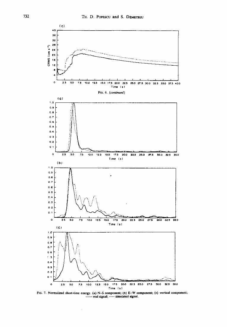
Short-time energy For nonstationary signals such as accelero-

grams, it is often more appropriate to consider a time-varying energy calculation such as the following:

M--1 E(n) = ~_~ [w,~y,_m] 2 (10)

rrl = O

where w,, is a weighting sequence of window which selects a segment of Yn and M is the number of samples in the window (M = 250).

This function shows the time-varying ampli- tude properties of the seismic signal. Figure 7 shows the energy function for original and simulated seismic signals for a Hamming window. It is easy to see the similarity between the analyzed signals.

730 TH. D . POPESCU and S. DEMETRIU

400

'¢~ 300

E 200

100

g o P - l o o

-200

- 3 0 0

- 4 0 0 0

(a)

V

_ _ iI I I I I I I I I i l I 1 I I

7.5 5 0 7 5 10.0 125 15.0 175 :~0.0 2 2 5 25.0 L:r?',5 30.0 325 35.0 37.5 40.0

Time ( s )

4O0

300

100

.f, o

-200

-300

-4 O0 0

{b)

i I 1

2.5 5.0 75 I I I f I I I | I l l i

10.0 12.5 ls .o 17.5 20 .0 22.5 2 5 0 27.5 30 .0 3 2 5 35.0 37.5 40 .0

T i m e ( s )

( c ) 400

v~ 3 O O

E 200 u 1 0 0

.g o

~ -~0o -2oo - 3 0 0 <

- 4 0 0 0 2~.s s'.o 71s ~ 10.0 125

I L , i i I i I I i i

15.0 17.5 20.0 22.5 25.0 27.5 30.0 32.5 35.0 37.5 40.0

Time i s )

FIG. 4. Evolution of simulated seismic signal. (a) N -S component; (b) E - W component; (c) vertical component.

1.0

0.9

0.8

0.7

0.6

0.5

0.4

0.3

0.2

0.1

(a )

* - - J I I 2,5 5 0 7.5 10.0

I t ! I I I I I I I I

12.5 15.o 17.s 20.0 22.5 2s.o 27.s 30.0 32.5 30.0 37.s 40.0

T i m e ( s )

FIG. 5. Normalized cumulative energy function. (a) N - S component; (b) E - W component; (c) vertical component. . real signal; . . . . simulated signal.

Analysis of ground motions using ARMA models 731

(b)

1.0

0.9

0.8

0 .7

0 .6

0 .5

0.4

0 .3

0.2

0.1

100

gO

80

6 0 E u 50

~ 4o

2O

10

70

~ . . . : °

I I I I I I I I I I I I I I I

2.5 5.0 r.5 I00 12.~ I~.0 I?.5 ZO.O ~.5 2~.0 :~r.5 3O.O 3Z~ 3~,.0 ~.~ 40.0

T ime (S )

(b)

0.4

0.3

0.2

0.1

1.0

0.9

0.8

0.7

0.6

0.5

I I I I I I I I , I, 2.5 5.0

"(C )

_ _ i ~ . J * ' ; " ~ I I I I I 2.5 5.0 7.5 10.0

7.5 10.0 Iz,5 1'~.0 17.5 20.0 22.5 zs.0 27,5 30.0 325 35.0 37,5 40o

T i m e ( s )

r

I I I I I I I I 12.5 150 I"r.5 20.0 225 25.0 27.5 30.0 32.5 35.0 37.5 40.0

T i m e ( s )

FIG. 5. (continued) (a)

6 3

5 6

49 e,

42 5

~ 2a (1:

14

| I I I I I I I I I I I I I I 2,5 5,0 7,5 10,0 lZ-~ 15.0 11",5 20.0 22,5 25,0 2?,5 30,0 32.5 35,0 37,5 40O

T i m e ( s )

Fro. 6. Cumulative r.m.s, acceleration. (a) N - S component ; (b) E - W component ; (c) vertical component ; real signal; . . . . simulated signal.

732 TH. D. POPESCU and S. DEMETRIU

4 0

(c) 3 6

3 2

28 7

ZO " ' ' " ' "

U 12

8

4

I I I I I I l I I I I

0 2,5 5,0 7`.5 10.0 12.5 15.0 17`.5 20.0 22.5 25.0 L:~.3 30.0 32,5 35.0 37`.5 40.0

T ime ( s )

FIG. 6. (continued)

( a l

1.0

0 . 8

0.7`

0 . 6

O.m, i

O, 4 ~"\~ 0 3

0.2

0.1

- - - J I I I '- ---~i - ' ~

O 2 . 5 5 . 0 7 .5 10.0 12,5 15.0 17`,5 20.0 22.5 25.0 z7.5 3o.0 32.5 35.0

T ime ( s )

( b )

1.o

0 .9

o.8

0.7`

0 .6

0 ,5

o , 4

0.3

0 2

0.1

G

:~: - ..,, : ",

j"j ~ .... 2.5 5.0 7`.5

( C I

lo.o 12.5 15.0 17` .~ 2o.o 22.5 2 s .o 27`.5 30.o 32.s 35.0

Time ( s )

1 .'0" ..;

o, \i 0.8

0 .6 ::,.

: 5

0,0.34 .,.. ,,..,, 0.2 ~ j .,..,

O. I ~,,... .... . .,," ......... I I I I I ..... " -~"'; -'-.~F'"'~. "~" .~"T~' -"t"- "''

0 2,5 S.O 7".5 10.0 12.5 15.0 17,5 200 225 25.0 27.5 30.0 32.5 35,0

T ime { s )

FIG. 7. N o r m a l i z e d sho r t - t ime energy. (a) N - $ c o m p o n e n t ; (b ) E - W c o m p o n e n t ; (c) ver t i ca l c o m p o n e n t ; real s igna l ; . . . . s i m u l a t e d s igna l .

Analysis of ground motions using A R M A models 733

(a) --~\ "--_____--~-

1 .0 [-x o.ol \-_

oo - o.'--~ 0.5 Lag (s)

..,.. --_,___ "-,...

"------__------

(b) -, ~ ~-V/"'--'--

o Oo.o, _i; c o ,

Log (s)

-'%,

- . , --,---.--._

( C ) " \ " ~ - - ' - - - ~ "

~02 0 [I"\ .... " ~ "

O0 ~ ,~ O0 0 . 2 0 .5

Log (s)

FIG. 8. Short-time autocorrelation function for recorded seismic signal. (a) N-S component; (b) E-W component; (c) vertical component.

Short-time autocorrelation analysis From the viewpoint of a stochastic repre-

sentation of the ground motion data, the autocorrelation function and the power spectral density provide statistical characterizations of the time series to be analyzed. The two functions are closely related to the second-order moments of a random process and are sufficient to provide a complete statistical description for a local Gaussian process like a segment of a motion earthquake accelerogram.

The conservation of stochastic properties of original and simulated seismic signal resulted,

also, from the representation of the evolutionary normalized correlation functions in Figs 8 and 9, respectively.

This function is computed for each stationary data block by:

where

ryy(k) = Ryy(k)/Ryy(O)

1 N - k

Ry,(k) = ~[ ~ [y, - )T][y,÷k -- )71

1 N k = 0 , 1 . . . . . K and )7 -- T, ~'~ y~.

IV i = l

(11)

734 TH. D. POPESCU and S. DEMETRIU

o o ~ " - - - " ~ 0.0 0.2 0.*~

Loci ( s )

( b )

2.o [ ~ 1. o ~ ' K ~"--'~-"" 0.5 o.o =._ .~--~'~--'-

o.o o.1 o.z 0.3 0.4 0.5 Lag (s)

-.-._.

°

--~ __-----_.~.

co,

2.0

1.0 k 0 .0 - - ' ~ - - ,

0.0 0.2 0.5 Laq (s)

F=G. 9. Short-time autocorrclation function for simulated seismic signal. (a) N-S component; (b) E - W component; (c) vertical component.

N is the number of samples for a stationary data block.

Short-time spectrum analysis Short-time spectrum analysis has traditionally

been one of the most important seismic signals processing techniques. The fundamental as- sumption underlying any short-time analysis method is that over a long-time interval, the signal is nonstationary, but that over a sufficiently short-time interval it can be con- sidered stationary.

The evaluation of power spectral density function for the original and simulated signals was performed by the relation:

I (-i2~'fk) 2 2 1 - ~ B k exp k=l - - ; 5 cr (12)

s(f) = 1 k=l~ Akexp(- i2~fk)

( -1 /2 ~<f ~< 1/2)

w h e r e Ak, B k represent ARMA parameters and o 2 is innovation variance.

The results are represented in Figs 10 and 11. Frequency peaks of spectra appear in a similar mode for both spectral representations, accord- ing to the evolution of the original accelerogram.

Starting from the results presented in this case

Analysis of ground motions using A R M A models 735

8

7

- . , 6

"-'5 n 4

/ 2

8

7

6

~4 ~3 o / 2

1

0

(a)

L--f--f

5 I0 15 20

Frequency (Hz)

(b)

A "~'--~ ---'~

O 5 10 15 20

Frequency (Hz)

(c)

0 5 10 15 20

Frequency (Hz)

FIG. 10. Short-time spectrum for recorded components of seismic signal. (a) N-S component; (b) E-W component; (c) vertical component.

o.

(a)

~ 10 15 20 Frequency (Hz)

(b)

, , ~ - _ _ ~ , , ~ . . . ~ - - - - - -

O 5 10 15 20

Frequency CHz]

FIO. 11. Short-time spectrum for simulated components of seismic signal. (a) N-S component; (b) E - W component; (c) vertical component.

736 TH. D. POPESCU and S. DEMETRIU

O

7

C6 5

O_ 4 o 3

~ 2 _J

1

(C) ~

... ~. -I",, "-,... x... --~--_.._~----_...__ ~--~.-:.---~- -~.. J \ . ~--...~_ .... ~ ~ '~ . . , . .~ - - ' - - , - - ~

-...

5 10 15 20 Frequency (Hz

FIG. 11. (continued)

study we can consider that the original and simulated signals are similar as concerns evolution in time and frequency, and are characterized by the same statistical properties of stationarity data blocks; the nonstationarity character of the original seismic signal is also conserved.

It may be emphasized that a complete agreement between the real and artificial accelerograms can never be expected since some approximations have been introduced while building the model and evaluating the parameters.

5. CONCLUSIONS

The analysis and simulation method presented in the paper seems to be a successful approach. Nonstationarity analysis technique and charac- terization of quasi-stationary data blocks of strong ground motions through parametric ARMA models provide an efficient and flexible description of the observed motion by a small number of parameters. The results presented in the case study, as well as other results obtained for several strong earthquake ground motions analyzed, are promising and could have sig- nificant utility in the design of engineering structures.

Potentially there are also other applications of the described approach to problems in aerody- namics, meteorological, oceanographic, wind, vibration and econometric data for nonstationary processes with both amplitude and frequency contents varying in time.

REFERENCES

Akaike, H. (1974). Markovian representation of stochastic processes and its application to the analysis of autoregres- sive moving average processes. Ann. Inst. Statist. Math. 26, 363-387.

Akaike, H. (1976). Canonical correlation analysis of time series and the use of an information criterion. In Lainiotis, D. G. and R. K. Mehra (Eds), System Identification: Advances and Case Studies. Academic Press, New York.

Akaike, H. (1977). On entropy maximization principle. Proc. Syrup. Applic. Statist., Wright State University, Dayton, OH. June 1976.

Akaike, H. (1978a). Time series analysis and control through

parametric models. In Findley, D. F. (Ed.), Applied time Series Analysis. Academic Press, New York.

Akaike, H. (1978b). A Bayesian extension of the minimum AIC procedure of autoregressive model fitting. Research Memo. No. 126, The Institute of Statistical Mathematics, Tokyo.

Akaike, H. (1978c). Likelihood of a model. Research Memo. No. 127, The Institute of Statistical Mathematics, Tokyo.

Bartlett, M. S. (1946). On the theoretical specification and sampling properties of autocorrelated time series. J. R. Statist. Soc., Series B, Vol. 27.

Cakmak, A. S. and R. I. Sheriff (1984). Parametric time series models for earthquake strong ground motions and their relationship to site parameters. Proc. 8th World Conf. on Earthquake Engng, 21-28 July, San Francisco, CA.

Chang, M. K., J. W. Kwiatkowski, R. F. Nau, R. M. Oliver and K. S. Pister (1979). ARMA models for earthquake ground motions. Report ORC 79-1, Operations Research Center, University of California, Berkeley.

Demetriu, S. (1986). EARTS---Program package for analysis and modelling of earthquake ground motions. Internal Report, Faculty of Civil Engineering, Bucharest, Romania.

Gersh, W. (1974). On the achievable accuracy of structural system parameter estimates. J. Sound Vibrat., 34, 63-79.

Gersh, W. and G. Kitagawa (1983). A time varying multivariate autoregressive modelling of econometric time series. Technical Paper 9, Statistical Research Division, Bureau of the Census, U.S. Department of Commerce.

Gersh, W. and G. A. Kitagawa (1985). Time varying AR coefficient model for modelling and simulating earthquake ground motion. Earthquake Engng Structural Dyn., 13, 243-254.

Gersh, W. and S. Luo (1970). Discrete time synthesis of randomly excited structural response. J. Acoust. Soc. Am., 51, 402-408.

Gersh, W., N. N. Nielsen and H. Akaike (1973). Maximum likelihood estimation of structural parameters from random vibration data. J. Sound Vibrat., 31, 295-308.

Golub, G. E. (1969). Matric decompositions and statistical calculations. In Milton, R. C. and J. A. Nelder Statistical Computation. Academic Press. New York.

Jennings, P. C., G. W. Housner and N. C. Tsai (1968). Simulated earthquake motions. Report of the Earthquake Engineering Research Laboratory, California Institute of Technology, Pasadena, CA.

Jones, R. H. (1975). Fitting autoregression. J. Am. Statist. Assoc. 70, 590-592.

Jurkevics, A. and T. J. Ulrich (1978). Representing and simulating of strong ground motions. Bull. SeL~mol. Soc. Am., 68, 781-801.

Kitada, Y, et al. (1983). Simulated earthquake ground motions by Gauss wave superposition method. Proc. 7th SMiRT, Vol. K(a), 53-61, Chicago.

Kitagawa, G. and H. Akaike (1978). A procedure for the modelling of nonstationary time series. Ann. Inst. Statist. Math., 30, B, pp. 351-363.

Kozin, F. (1979). Estimation and modelling of non-stationary time series. Proc. Symp. Comput. Meth. Engng, University of Southern California, pp. 603-612.

Ana lys i s o f g r o u n d m o t i o n s us ing A R M A m o d e l s 737

Nau, R. F. and R. M. Oliver (1979). Adaptive filtering revisited. I. Operat. Res. Soc., 30, 825-831.

Nau, R. F., R. M. Oliver and K. S. Pister (1980). Simulating in analysing artificial non-stationary earthquake ground motions. Report UCB/EERC-80/36, University of Cali- fornia, Berkeley.

Ozaki, T. and H. Tong (1975). On the fitting of non-stationary autoregressive models in time series analysis. Proc. 8th Hawaii Int. Conf. Syst. Sci., Western Periodical Company, Hollywood, CA.

Polhemus, N. W. and A. S. Cakmak (1981). Simulation of earthquake ground motions using autoregressive moving average (ARMA) models. Earthquake Engng Structural Dyn. 9, 343-354.

Popcscu, Th. D. (1981) TIMES--Program package for time series analysis and forecasting. Internal Report, Central

Institute for Management and Informatics, Bucharest, Romania.

Popescu, Th. D. (1985). AUTOB & J--A computer-aided procedure for time series analysis and forecasting. Preprints 3rd IFAC Syrup. Computer Aided Design in Control and Engng Syst., 31 July-2 August, Lyngby, Denmark.

Shibata, R. (1976). Selection of the order of an autoregressive model by Akaike's information criterion. Biometrika, 63, 117-126.

Tertisco, M., P. Stoica and Th. D. Popescu (1985). Time Series Modelling and Forecasting (in Romanian). Acade- mic Publishing House, Bucharest.

*** Digitized Data of Strong Motion Earthquake Accelero- grams in Romania, 4 March 1977. Building Research Institute, Tokyo, 1977.