Analysis and Simulation of Blood Flow in the Portal Vein ... · Analysis and Simulation of Blood...

Analysis and Simulation of Blood Flow in the Portal Vein with

Uncertainty Quantification

João Pedro Carvalho Rêgo de Serra e Moura

Master Thesis on

Aerospace Engineering

Júri

Presidente: Prof. Fernando Lau

Supervisor: Dr. José Manuel da Silva Chaves Ribeiro Pereira

Co-supervisor: Prof. José Carlos Fernandes Pereira

Vogais: Prof. Carlos Bettencourt da Silva

Prof. Pedro Álvares Serrão

October 2011

“Livers are important, Cuddy. You can’t live without them, hence the name. ”

Dr. Gregory House1

1Character of tv series House M.D. by James Blake.

Agradecimentos

Nesta secção gostaria de deixar explícito o meu agradecimento a algumas pessoas, que sem o seu contri-

buto não teria sido possível elaborar este trabalho.

Em primeiro lugar gostaria de agradecer ao Dr. José Manuel Pereira pela sempre enorme disponibilidade

em ajudar, quer na partilha de ideias, quer pelos sempre pertinentes comentários.

Agradeço ao Prof. José Carlos Pereira pelas sessões de brainstorming e de ajuda na construção do docu-

mento.

À Rita Ervilha quero agradecer a paciência em me explicar o processo estocástico e toda a disponibilidade

durante o projecto. À restante equipa do LASEF, agradeço a ajuda em todas as dificuldades encontradas e

à companhia durante todo este tempo.

Por fim, à Ana Antunes, pela paciência durante este tempo todo e por me ter motivado ao longo do decorrer

do projecto.

Abstract

Blood flow simulations in CFD are seen as a very attractive solution for diagnosing diseases. The

main objective of this work is to simulate blood flow in the portal vein for patients with liver cirrho-

sis and to quantify the uncertainty that surrounds blood flow. Initially all the tools required were

explored: the verification and validation of the models were performed as well as convergence

studies.

Moreover an uncertainty quantification process was used based on a Non-Intrusive Spectral

Method. The sources of uncertainty were researched and quantified as the geometry and blood

model were assumed as the main random variables.

Key Words: Blood flow, CFD, uncertainty quantification, Non-Intrusive Spectral Projection.

Resumo

As simulações do escoamento de sangue em CFD são vistas como soluções muito atractivas

para diagnosticar doenças. O objectivo principal deste trabalho é simular o escoamento de

sangue na veia porta de doentes com cirrose do ígado e quantificar a incerteza que envolve o

escoamento de sangue. Inicialment foram desenvolvidas todas as ferramentas necessárias: foi

realizada a verificação e validação dos modelos assim como os estudos de convergência.

Para além disso o modelo de quantificação de incerteza foi baseado num método de projeção

espectral não intrusivo. As fontes de incerteza foram pesquisadas e quantificadas, sendo que o

modelo de sangue e a geomtria foram consideradas as principais fontes de incerteza.

Palavras chave: escoamento de sangue, CFD, quantificação de incerteza, método de projeção

espectral não intrusiva.

Contents

List of Figures V

List of Tables VII

Acronyms IX

Symbols XI

1 Introduction 1

1.1 Problem under Consideration . . . . . . . . . . . . . . . . . . . . . . . . . . . . . . . . . . . . 1

1.1.1 Liver . . . . . . . . . . . . . . . . . . . . . . . . . . . . . . . . . . . . . . . . . . . . . 2

1.1.2 Physiology of Blood Vessels . . . . . . . . . . . . . . . . . . . . . . . . . . . . . . . . 3

1.1.3 Hemorheology . . . . . . . . . . . . . . . . . . . . . . . . . . . . . . . . . . . . . . . . 4

1.1.4 Image Acquisition and Integration with CFD . . . . . . . . . . . . . . . . . . . . . . . . 7

1.2 Literature Survey . . . . . . . . . . . . . . . . . . . . . . . . . . . . . . . . . . . . . . . . . . 8

1.3 Objectives . . . . . . . . . . . . . . . . . . . . . . . . . . . . . . . . . . . . . . . . . . . . . . 8

1.4 Organization of the Dissertation . . . . . . . . . . . . . . . . . . . . . . . . . . . . . . . . . . 9

2 Mathematical and Numerical Model 11

2.1 Modeling Blood Flow . . . . . . . . . . . . . . . . . . . . . . . . . . . . . . . . . . . . . . . . 11

2.2 Continuity and Momentum Equations . . . . . . . . . . . . . . . . . . . . . . . . . . . . . . . 12

2.3 Non-Newtonian Models . . . . . . . . . . . . . . . . . . . . . . . . . . . . . . . . . . . . . . . 12

2.4 Numerical Model . . . . . . . . . . . . . . . . . . . . . . . . . . . . . . . . . . . . . . . . . . 14

2.4.1 Methodology . . . . . . . . . . . . . . . . . . . . . . . . . . . . . . . . . . . . . . . . . 15

2.4.2 Governing Equations . . . . . . . . . . . . . . . . . . . . . . . . . . . . . . . . . . . . 15

2.4.3 Spatial Discretization Methods . . . . . . . . . . . . . . . . . . . . . . . . . . . . . . . 16

2.4.4 Meshing . . . . . . . . . . . . . . . . . . . . . . . . . . . . . . . . . . . . . . . . . . . 17

2.4.5 Boundary Conditions . . . . . . . . . . . . . . . . . . . . . . . . . . . . . . . . . . . . 18

2.4.6 Algorithms for the Solution of the Incompressible Conservation Equations . . . . . . . . 18

2.4.7 Star-CCM+® . . . . . . . . . . . . . . . . . . . . . . . . . . . . . . . . . . . . . . . . . 19

I

3 Uncertainty Quantification Process 21

3.1 Polynomial Chaos . . . . . . . . . . . . . . . . . . . . . . . . . . . . . . . . . . . . . . . . . . 21

3.1.1 Askey-Scheme . . . . . . . . . . . . . . . . . . . . . . . . . . . . . . . . . . . . . . . 22

3.2 Non Intrusive Spectral Projection . . . . . . . . . . . . . . . . . . . . . . . . . . . . . . . . . . 22

4 Verification and Validation 27

4.1 Verification . . . . . . . . . . . . . . . . . . . . . . . . . . . . . . . . . . . . . . . . . . . . . . 27

4.1.1 Methods . . . . . . . . . . . . . . . . . . . . . . . . . . . . . . . . . . . . . . . . . . . 27

4.1.2 Results . . . . . . . . . . . . . . . . . . . . . . . . . . . . . . . . . . . . . . . . . . . . 29

4.2 Validation . . . . . . . . . . . . . . . . . . . . . . . . . . . . . . . . . . . . . . . . . . . . . . 31

4.2.1 Methods . . . . . . . . . . . . . . . . . . . . . . . . . . . . . . . . . . . . . . . . . . . 31

4.2.2 Results . . . . . . . . . . . . . . . . . . . . . . . . . . . . . . . . . . . . . . . . . . . . 33

5 Results 35

5.1 Deterministic Model . . . . . . . . . . . . . . . . . . . . . . . . . . . . . . . . . . . . . . . . . 35

5.1.1 Geometry and Convergence Analysis . . . . . . . . . . . . . . . . . . . . . . . . . . . 35

5.1.2 Newtonian and Non-Newtonian Deterministic Model . . . . . . . . . . . . . . . . . . . 36

5.2 Stochastic Influence of the Thrombosis Radius . . . . . . . . . . . . . . . . . . . . . . . . . . 37

5.2.1 Small Obstruction . . . . . . . . . . . . . . . . . . . . . . . . . . . . . . . . . . . . . . 37

5.2.2 Critical Radius . . . . . . . . . . . . . . . . . . . . . . . . . . . . . . . . . . . . . . . . 43

5.3 Stochastic Influence of the Blood Viscosity . . . . . . . . . . . . . . . . . . . . . . . . . . . . 45

5.3.1 Model Uncertainty . . . . . . . . . . . . . . . . . . . . . . . . . . . . . . . . . . . . . . 45

5.3.2 Model Parameters Uncertainty . . . . . . . . . . . . . . . . . . . . . . . . . . . . . . . 45

5.3.3 Distinctive Models . . . . . . . . . . . . . . . . . . . . . . . . . . . . . . . . . . . . . . 51

5.4 Blood and Geometry Stochastic Influence . . . . . . . . . . . . . . . . . . . . . . . . . . . . . 53

5.4.1 Smaller Radius and Model Parameters Uncertainty . . . . . . . . . . . . . . . . . . . . 53

5.4.2 Critical Radius and Model Parameters Uncertainty . . . . . . . . . . . . . . . . . . . . 53

6 Conclusions 59

A Probability Density Functions 67

B Numerical Methods 69

B.1 Gauss-Legendre Quadrature . . . . . . . . . . . . . . . . . . . . . . . . . . . . . . . . . . . . 69

B.2 Gauss-Hermite Quadrature . . . . . . . . . . . . . . . . . . . . . . . . . . . . . . . . . . . . . 69

B.3 Gauss-Jacobi Quadrature . . . . . . . . . . . . . . . . . . . . . . . . . . . . . . . . . . . . . . 70

C Parameter Influence in the Blood Carreau Model 71

II

List of Figures

1.1 Human Liver . . . . . . . . . . . . . . . . . . . . . . . . . . . . . . . . . . . . . . . . . . . . . 2

1.2 The portal vein and its tributaries . . . . . . . . . . . . . . . . . . . . . . . . . . . . . . . . . . 3

1.3 Hematocrit vs Apparent Viscosity (Robertson et al. [2008]) . . . . . . . . . . . . . . . . . . . . 6

2.1 Strain Rate vs Apparent Viscosity . . . . . . . . . . . . . . . . . . . . . . . . . . . . . . . . . 14

2.2 Fluxogram of the SIMPLE algorithm . . . . . . . . . . . . . . . . . . . . . . . . . . . . . . . . 20

3.1 Askey family of orthogonal polynomials and its relation with the Hypergeometric series . . . . 22

4.1 Cylindrical Duct . . . . . . . . . . . . . . . . . . . . . . . . . . . . . . . . . . . . . . . . . . . 28

4.2 Velocity field in the XY plane . . . . . . . . . . . . . . . . . . . . . . . . . . . . . . . . . . . . 28

4.3 Velocity profiles of the Newtonian and Non-Newtonian flows . . . . . . . . . . . . . . . . . . . 29

4.4 Mesh convergence of the velocity profile . . . . . . . . . . . . . . . . . . . . . . . . . . . . . . 30

4.5 Zoom of Fig.4.4 . . . . . . . . . . . . . . . . . . . . . . . . . . . . . . . . . . . . . . . . . . . 30

4.6 Mesh Convergence in Log scale for a 3D cylindrical duct: PNN 2nd - Polyhedric mesh, Non-

Newtonian, 2nd order scheme; TNN 2nd - Trimmed mesh , Non-Newtonian, 2nd order scheme;

PN 2nd - Polyhedric mesh, Newtonian, 2nd order scheme PN 1st - Polyhedric mesh, Newto-

nian, 1st order scheme 1st - real 1st order scheme . . . . . . . . . . . . . . . . . . . . . . . . 31

4.7 Mesh Convergence in Log scale for a 2D cylindrical duct . . . . . . . . . . . . . . . . . . . . . 32

4.8 Graft Geometry . . . . . . . . . . . . . . . . . . . . . . . . . . . . . . . . . . . . . . . . . . . 32

4.9 Axial velocity field in the XY plane . . . . . . . . . . . . . . . . . . . . . . . . . . . . . . . . . 33

4.10 Axial velocity field in the XZ plane . . . . . . . . . . . . . . . . . . . . . . . . . . . . . . . . . 33

4.11 Velocity profiles along X in the XY plane . . . . . . . . . . . . . . . . . . . . . . . . . . . . . . 34

4.12 Velocity profiles along X in the XZ plane . . . . . . . . . . . . . . . . . . . . . . . . . . . . . . 34

5.1 Geometry of the Portal Vein Model . . . . . . . . . . . . . . . . . . . . . . . . . . . . . . . . . 36

5.2 Convergence Graphic of a Velocity profile in the left branch after the clot for different sized

meshes . . . . . . . . . . . . . . . . . . . . . . . . . . . . . . . . . . . . . . . . . . . . . . . 37

5.3 Fluxogram of the stochastic process . . . . . . . . . . . . . . . . . . . . . . . . . . . . . . . . 38

5.4 Bar Chart of the Strain Rate values in the model . . . . . . . . . . . . . . . . . . . . . . . . . 39

III

5.5 Absolute difference of the velocity fieldbetween a Newtonian and a Non-Newtonian blood model 39

5.6 Velocity field of the Non-Newtonian blood model . . . . . . . . . . . . . . . . . . . . . . . . . 39

5.7 PDF for the Shear with the radius as a random variable . . . . . . . . . . . . . . . . . . . . . . 40

5.8 Shear expansion coefficients with the radius as a random variable . . . . . . . . . . . . . . . . 41

5.9 Stochastic parameters of the velocity profile for different small thrombosis radius . . . . . . . . 41

5.10 PDF for the Pressure at the inlet with the thrombosis with the radius as a random variable . . . 42

5.11 Average of the velocity field with the radius as a random variable . . . . . . . . . . . . . . . . 42

5.12 Standard deviation of the velocity field with the radius as a random variable . . . . . . . . . . . 42

5.13 Stochastic parameters of the velocity profile for different thrombosis radius . . . . . . . . . . . 43

5.14 PDF for the Shear with the radius as a random variable . . . . . . . . . . . . . . . . . . . . . . 44

5.15 PDF for the Pressure at the inlet with the thrombosis with the radius as a random variable . . . 44

5.16 PDF for the Pressure at the inlet with the blood model as a random variable . . . . . . . . . . 46

5.17 Shear expansion coefficients with the blood model as a random variable . . . . . . . . . . . . 47

5.18 PDF for the Shear with the blood model as a random variable . . . . . . . . . . . . . . . . . . 47

5.19 Average of the velocity field with the blood model as a random variable . . . . . . . . . . . . . 48

5.20 Standard deviation of the velocity field with the blood model as a random variable . . . . . . . 48

5.21 PDF for the Shear with the blood model parameters as random variables . . . . . . . . . . . . 49

5.22 PDF for the Pressure at the inlet with the blood model parameters as random variables . . . . 49

5.23 Average of the velocity field with the blood model parameters as random variables . . . . . . . 50

5.24 Standard deviation of the velocity field with the blood model parameters as random variables . 50

5.25 PDF for the Shear with the blood model as a random variable . . . . . . . . . . . . . . . . . . 51

5.26 PDF for the Pressure at the inlet with the with the blood model as a random variable . . . . . . 52

5.27 Average of the velocity field with the blood model as a random variable . . . . . . . . . . . . . 52

5.28 Standard deviation of the velocity field with the blood model as a random variable . . . . . . . 52

5.29 Stochastic parameters of the velocity profile with the thrombosis radius and the blood model

parameters as random variables . . . . . . . . . . . . . . . . . . . . . . . . . . . . . . . . . . 54

5.30 PDF for the Pressure at the inlet with the thrombosis radius and the blood model parameters

as random variables . . . . . . . . . . . . . . . . . . . . . . . . . . . . . . . . . . . . . . . . . 54

5.31 PDF for the Shear with the thrombosis radius and the blood model parameters as random

variables . . . . . . . . . . . . . . . . . . . . . . . . . . . . . . . . . . . . . . . . . . . . . . . 55

5.32 Shear expansion coefficients with the radius and the blood model parameters as random vari-

ables . . . . . . . . . . . . . . . . . . . . . . . . . . . . . . . . . . . . . . . . . . . . . . . . . 55

5.33 Stochastic parameters of the velocity profile with the thrombosis radius and the blood model

parameters as random variables . . . . . . . . . . . . . . . . . . . . . . . . . . . . . . . . . . 56

5.34 PDF for the Shear with the thrombosis radius and the blood model parameters as random

variables . . . . . . . . . . . . . . . . . . . . . . . . . . . . . . . . . . . . . . . . . . . . . . . 57

IV

5.35 PDF for the Pressure at the inlet with the thrombosis radius and the blood model parameters

as random variables . . . . . . . . . . . . . . . . . . . . . . . . . . . . . . . . . . . . . . . . . 57

5.36 Shear expansion coefficients with the radius and the blood model parameters as random vari-

ables . . . . . . . . . . . . . . . . . . . . . . . . . . . . . . . . . . . . . . . . . . . . . . . . . 58

A.1 Probability density functions . . . . . . . . . . . . . . . . . . . . . . . . . . . . . . . . . . . . 68

C.1 Study on the influence of µ0 . . . . . . . . . . . . . . . . . . . . . . . . . . . . . . . . . . . . 71

C.2 Study on the influence of µ∞ . . . . . . . . . . . . . . . . . . . . . . . . . . . . . . . . . . . . 72

C.3 Study on the influence of λ . . . . . . . . . . . . . . . . . . . . . . . . . . . . . . . . . . . . . 72

C.4 Study on the influence of n . . . . . . . . . . . . . . . . . . . . . . . . . . . . . . . . . . . . . 72

C.5 Study on the combined influence of µ0, µ∞ and n . . . . . . . . . . . . . . . . . . . . . . . . 73

V

List of Tables

2.1 Blood models parameters. . . . . . . . . . . . . . . . . . . . . . . . . . . . . . . . . . . . . . 15

3.1 Orthogonal polynomials of the Askey family and their respective weighting functions . . . . . . 23

3.2 Main information for Hermite, Jacobi and Legendre unidimensional polynomial sets. . . . . . . 23

4.1 Mesh parameters . . . . . . . . . . . . . . . . . . . . . . . . . . . . . . . . . . . . . . . . . . 30

5.1 Model dimensions (Petkova et al. [2003]) . . . . . . . . . . . . . . . . . . . . . . . . . . . . . 36

5.2 Mean and standard deviation values with the radius as a random variable. . . . . . . . . . . . 40

5.3 Mean and standard deviation values with the radius as a random variable. . . . . . . . . . . . 44

5.4 Blood models parameters for the stochastic process. . . . . . . . . . . . . . . . . . . . . . . . 46

5.5 Mean and standard deviation values with the blood model as a random variable. . . . . . . . . 48

5.6 Mean and standard deviation values with the blood model parameters as random variables. . . 50

5.7 Mean and standard deviation values with the blood model as a random variable. . . . . . . . . 51

5.8 Mean and standard deviation values with the thrombosis radius and the blood model parame-

ters as random variables. . . . . . . . . . . . . . . . . . . . . . . . . . . . . . . . . . . . . . . 53

5.9 Mean and standard deviation values with the thrombosis radius and the blood model parame-

ters as random variables. . . . . . . . . . . . . . . . . . . . . . . . . . . . . . . . . . . . . . . 56

VII

Acronyms

CFD Computational Fluid Dynamics

CI Condence Interval

MAC Marned and Cell

MRI Magnetic Resonance Imaging

NISP Non Intrusive Spectral Projection

PC Polynomial Chaos

PDF Probability Distribution Function

RBC Red Blood Cell

SNR Signal-to-Noise Ratio

SIMPLE Semi-Implicit Method for Pressure Linked Equations

WBC White Blood Cell

IX

Symbols

cfj Spectral Modes

D Diameter [m]

Ht Hematocrit [%]

In Orthogonal Polynomial

k Flow Consistency Index [Pa.s]

n Power Law Index

p Pressure [Pa]

Q Mass Flow Rate [kg/s]

Re Reynolds Number

Sm Mass Residue

V Velocity [m/s]

Superscript

¯ mean quantity

~ vector

XI

Greek symbols

α Womersley Number

γ Strain Rate Tensor Modulus [1/s]

η Casson Rheological Constant

λ Relaxation Time [s]

µ Blood Viscosity [Pa.s]

µ0 Zero Shear Rate Limit Viscosity [Pa.s]

µ∞ Innite Shear Rate Limit Viscosity [Pa.s]

ξ Random Variable

ρ Fluid Density [kg/m3]

τ0 Yield Stress [Pa]

φ Scalar Field

φj Shape Function

ω Angular Frequency [rad/s]

Ω Control Volume

XII

Chapter 1

Introduction

The first chapter of this dissertation serves motivational purposes for this work and provides some background

on the subject in study. Furthermore the objectives proposed for this Thesis are presented as well as an

outline of the Thesis itself.

1.1 Problem under Consideration

Nowadays with the proliferation of computers and the increase in their computational capability, Computa-

tional Fluid Dynamics (CFD) is becoming a wide-spread tool in several applications. This associated with the

society’s desire in increasing the human being’s longevity has led to the combination of CFD and medicine.

In fact, over the last decade, CFD has become a powerful and important tool to study the cardiovascular

system.

People all over the world suffer from a disease called liver cirrhosis, a disease that can by itself cause an

increase in the mortality risk and reduce the patient’s quality of life. One problem associated with this disease

is the rupture and bleeding of small blood vessels, due to the reduction of blood flow in the portal vein, which

makes the pressure rise on the wall, forcing blood coming from the intestines around small vessels. These

blockages originate blood recirculation within the portal vein increasing the wall shear stress as their size

increases.

Due to the significance of the blockages in the blood vessels in blood flow, accurate techniques are required

to acquire images from the patient’s body. However these techniques are still limited to an accuracy of about

0.3 mm, which may represent about 10% of the occlusion’s size.

Blood has a shear-thinning behaviour and is therefore modeled as a Non-Newtonian fluid. However this

behaviour is still not totally agreed upon the scientific community as there are several models to simulate this

behaviour, with no certainty in which one best represents the behaviour of the blood viscosity.

Within this context, the development of a numerical model for the blood flow in the portal vein with uncertainty

in the geometry and the blood viscosity has been proposed. This research was motivated by the need to pro-

1

duce accurate predictions of blood flow in a diseased portal vein considering several uncertainty parameters

that affect its blood flow.

This section provides some contextualization to the liver, taking a closer look at the portal vein as well as a

description of blood vessels. Furthermore hemorheology and some image acquisition techniques are here

presented.

1.1.1 Liver

The liver is the most important gland of the digestive tract due to its large number of metabolic functions,

indispensable to life. This is the most voluminous organ of the human body, located in the supramesocolic

abdominal cavity. It has an external secretion, bile, which is launched in the second portion of the duodenum

through the bile ducts, and an internal secretion, by which blood reaches the inferior vena cava (Esperança

Pina [2004]).

General Considerations

The liver lies beneath the diaphragm in the abdominal-pelvic region of the abdomen and above the right

kidney. Consisting of a left anatomical lobe and a more voluminous right anatomical lobe, the liver has an

asymmetric ovoid shape (Fig. 1.1).

Figure 1.1: Human Liver

The liver is the heaviest of the viscera. This organ has the the greatest differences from person to person as

its weight and shape change continuously with age. It can weight from 0.8 to 2.5 kg.

With a reddish-brown colour, its consistency, even though solid, is depressive showing marks of the neigh-

boring viscera (Millet-Bex [2005]).

Liver Function

The liver is essential to human life, and although there is a possibility of short-term dialysis, there are no

means of replacing the liver functions. These functions include filtering the blood that comes from the di-

2

gestive track, before passing through the rest of the body, glycogen storage, decomposition of red blood

cells (RBCs), plasma protein synthesis, hormone production and detoxification.

Portal Vein

The portal vein originates from two main roots, the spleno-mesenteric venous trunk after meeting with the

splenic vein inferior mesenteric vein and superior mesenteric vein as seen in Fig. 1.2. The portal vein at the

level of the hepatic hilum, splits into two terminal branches, according to a variable angle, the right portal vein

and left portal vein. The caudate lobe vein or Spiegel’s arises as a branch of the right portal vein or left portal

vein, or rarely as a terminal branch of the portal vein’s trunk.

Figure 1.2: The portal vein and its tributaries

Liver Cirrhosis

In cirrhosis, damaged liver cells get replaced by fibrous tissue, and the regeneration of liver cells does not

follow the normal process but rather forms nodules surrounded by that fibrous tissue. Fibrous tissue causes

an increase in resistance, leading to a decrease of blood flow to and through the organ (Petkova [2008]).

1.1.2 Physiology of Blood Vessels

The human circulatory system is a remarkable example of the effectiveness of the body mechanisms, with

the vascular system playing the role of transporting blood and exchanging blood constituents with the body

tissues. The vascular system has three different types of blood vessels: arteries, veins and capillaries. They

all show a structure with a central opening, the lumen, surrounded by a three layered wall: the tunica intima,

the vessel’s thinnest layer, is a single layer of squamous endothelial cells facing the blood; the tunica media,

the thickest layer, which consists of elastic fibre, connective tissue and polysaccharide substances; and the

tunica adventitia, which consists of connective tissue and nerves.

Arteries are blood vessels that come from the heart towards the periphery, transporting oxygenated blood,

whereas veins, with thinner layers, perform the inverse route with deoxygenated blood. Capillaries are tiny

blood vessels that supply tissues with components of blood and carried by blood.

3

Blood vessels deteriorate with aging. In a normal aging process, they tend to get wider and with a more

tortuous path. The most common disease is atherosclerosis.

Atherosclerosis

Atherosclerotic cardiovascular disease is a leading cause of mortality in the industrialized world (Boyd et al.

[2007]). A fatty substance, the cholesterol, is the main factor for the appearance of atherosclerosis. When

the concentration of this fatty material, which comes from food and from the liver, increases in the blood, it

will be deposited in the curves and branches of the circulatory system, making it difficult for fast blood flow.

Hemodynamic factors, such as the wall shear stress, particle residence time, recirculation zone, arterial wall

strain and wall compliance, play important roles in the regulation of vascular biology and the localization

of atherosclerosis, which is usually attributed to various forms of endothelial dysfunction (Buchanan et al.

[1999]).

There are some risk factors to this disease. In fact, the patient’s physiological, biochemical and genetic make-

up can contribute to this disease as well as some lifestyle factors such as heavy alcohol abuse, smoking and

diet.

This condition can cause hypertension, coronary heart disease, heart attack, infarction, which is caused by

thrombosis, and too little blood to the legs and feet.

Thrombosis

Thrombosis is the formation of a blood clot, called a thrombus, inside a living blood vessel. The mechanisms

of thrombosis are identical to the mechanisms of hemostasis, the clotting system that protects the body from

excessive blood loss. Thrombosis is very dangerous for a human being, as it will increase the wall shear

stress in the blood vessel where it occurring as well as an increase in local velocity and deflection of blood

flow through healthier blood vessels.

1.1.3 Hemorheology

Hemorheology is the science that deals with the mechanics involving blood flow and the deformation of blood

and its components. The study of hemorheology involves both the inspection of macroscopic and microscopic

blood properties.

Blood Function

Blood flows through the human body with the purpose of taking oxygen and nutrients to all tissues, removing

waste and carbon dioxide from our body. The circulation of this fluid is assured by both the heart and the

blood’s mechanical properties.

4

Blood Constitution

Blood is a concentrated suspension of formed elements that includes red blood cells (RBCs) or erythrocytes,

white blood cells (WBCs) or leukocytes, and platelets (Popel and Johnson [2005]).

Plasma consists of mostly water and its major role is to transport dissolved substances.

Erythrocytes are cells with an almost saturated solution of hemoglobin in water, hence the red color, as

well as inorganic elements. These cells are mostly involved in oxygen and carbon dioxide transport. Its

volume concentration in whole blood has a great impact on the blood rheological properties and its called the

Hematocrit (Ht).

The Leukocytes are the human body’s vital tool in fighting infection through destroying bacteria and virus and

forming antibodies and sensitized lymphocytes. These cells’ influence on the blood rheology is negligible,

except for really small vessels.

Platelets, also known as thrombocytes, constitute the third solid blood element. With a rounded shape they

are tiny and do not have a nucleus as they are not complete cells, only cellular fragments. Platelets are

responsible for stopping bleeding thus blood loss.

Rheological Properties

Whole blood shows a Non-Newtonian behaviour explained by three factors: the ability of RBCs forming three-

dimensional micros-structures at low shear rates, their deformability and their tendency to align with the flow

field at high shear rates.

The factors that influence hemodynamics are extensive and complex such as flow separation (when speed

of the boundary layer relative to the object falls almost to zero), flow recirculation (area of flow composed

of eddies), oscillatory wall shear stress, circulating fluid volume, vascular diameter, resistance and blood

viscosity. Blood vessel geometry and orientation are important determinants of the effects of hemorheological

alterations on flow resistance (Baskurt et al. [2004]).

As the heart pulsates blood at a certain frequency, the blood that flows from that organ has a pulsatile

behaviour. However as the blood flows to the rest of the body and the blood vessels get thinner, the blood flow

assumes a steady state behaviour. To know whether the flow is closer to steady or pulsatile behaviour two

parameters are measured. Those parameters are the Reynolds number (Re) and the Womersley number (α),

given by equations 1.1 and 1.2, where ρ is the blood density, V the mean velocity, D the diameter of the blood

vessel, ω the angular frequency and µ the blood viscosity.

Additionally there are important physiological factors that also affect the rheological properties such as dis-

eases, drugs, excess weight and diet.

Re =ρV D

µ(1.1)

α =D

2

√ρω

µ(1.2)

5

Whole Blood Viscosity

The whole blood viscosity is the most well studied property of blood. It shows a Non-Newtonian behaviour,

where the viscosity decreases with increasing shear rate.

Blood viscosity can be defined as the quantity that describes the blood’s resistance to flow, which is being

deformed by either shear stress or tensile stress. The common SI unit of viscosity is the Pascal second

(Pa.s).

For different parts of the circulatory system, different behaviours of blood viscosity seem to happen. In healthy

straight large blood vessels, where the blood flow is in high strain rate blood shows Newtonian behaviour, how-

ever, in small blood vessels, the strain rate is low and the blood viscosity shows a shear-thinning behaviour.

This behaviour is explained by the deformation and aggregation of RBCs. Since blood is composed of a

suspension of many elements of varying size, when at low strain rates, blood thickens as a consequence of

RBCs aggregation, also known as roulleaux formation (Marossy et al. [2009]). These structures are reversible

with an increase in the strain rate.

The hematocrit and blood components play a major role on blood viscosity. In fact, Fig. 1.3 shows the

increase of blood viscosity with the increase of the hematocrit. The blood temperature also has an effect on

its viscosity as, for the same hematocrit, for a decrease in temperature there is a significant increase in the

viscosity.

Figure 1.3: Hematocrit vs Apparent Viscosity (Robertson et al. [2008])

Viscoelasticity of Blood

Viscoelastic fluids are viscous fluids which have the ability to store and release energy ( Robertson et al.

[2008]). They resist to shear flow and strain when stress is applied, but also return to the original state when

stress is removed.

This property appears in blood as the 3D micro-structure of RBCs tend to store energy as well as release it.

There are several models to represent the viscoelastic behaviour of blood such as the Oldroyd-B model, the

Yeleswarapu model and the model from Phillips and Deutsch.

6

The viscoelastic behaviour shows little influence on steady blood flow and, therefore it is disregarded in most

of the blood models used for computational fluid dynamics (CFD) analysis.

Disease states

The mechanical properties of blood are very much influenced by the patient’s health. In fact, various diseases

change the blood rheology such as diabetes, myocardial infarction, hypertension and rheumatic diseases.

One effect that is usually common to all these diseases is the increase in the blood viscosity.

The increase in the blood viscosity might be due to an increase in the hematocrit, plasma hyperviscosity,

hyperaggregation of RBCs, a decrease in RBC deformability or even an increase in blood’s cholesterol levels.

The cholesterol levels are not constant throughout the day, as after a big meal the levels rise and after sleep

the levels lower. Since an increase in cholesterol levels mean an increase in blood viscosity (Rosenson et al.

[2002]), there is an inherent uncertainty in blood viscosity for a patient on a daily basis.

On the other hand, the hematocrit, which also has a direct influence in blood viscosity, differs from person

to person with greater differences when considering different genders (Kameneva et al. [1998]). These

differences inflict uncertainty in blood viscosity on a patient basis.

1.1.4 Image Acquisition and Integration with CFD

With the promising results obtained from CFD simulations on simplified geometries, reconstructing accurate

patient-specific three-dimensional models of blood vessels for CFD integration are mostly desired (Antiga

et al. [2003]). There are several methods used to acquire images from the human body, which are then

processed and integrated into CFD simulations. The most common method is the magnetic resonance

imaging (MRI), which consists in using a powerful magnetic field to align the magnetization of some atoms in

the body, and radio frequency fields to systematically alter the alignment of this magnetization, which is then

used to reconstruct an image of the scanned area of the body. This method has a limited resolution, in the

order of 0.3 mm (Milner et al. [1998]).

The methods of image acquisition and CFD integration carry errors that may come from both the MRI and

the reconstruction procedure. In the MRI, apart from the limited resolution, there is an intrinsic trade-off be-

tween the signal-to-noise ratio (SNR), the spatial resolution and the acquisition time required by the intended

clinical/research application (Nowak [1999]). Bearing in mind that the MRIs are done on in vivo patients, the

actual movement of the patients must be taken into account and therefore the longer the exam lasts, the less

accurate will it be, so it is desirable to have it done as quick as possible. However if the SNR is too small or

the contrast too low it becomes very difficult to detect anatomical structures, because tissue characterization

fails (Gerig et al. [1992]).

From the MRI to a computational model, the images of the 3D geometry go through a process of image

segmentation, surface extraction, and finally surface smoothing (Gambaruto et al. [2011]). The image seg-

mentation can be done in three ways: manual, semi-automatic or automatic. From the work of Bazille et al.

[1994] it is clear that there are errors associated with each method, thus leading to virtual geometry variance.

Since there will always be some noise in the images, there are smoothing tools to eliminate it. It is clear in the

work of Gambaruto et al. [2011] that using different smoothing levels will yield in different geometries, which

will invariably lead to different blood flow simulations.

7

1.2 Literature Survey

In the last two decades, the scientific community has been developing several techniques and models, allow-

ing the integration of CFD analysis in the human blood. In this section is presented an overview of recent

studies in CFD simulations of blood flow with special emphasis on the portal vein and the uncertainty regard-

ing blood and geometry modeling. Furthermore some work on uncertainty quantification is also referred.

Yang et al. [2006] propose an approach for developing patient-specific 3D models of portal veins to provide

geometric boundary conditions for CFD, based on MRI. On this note, Botar et al. [2010] use actual patient

imaging of the portal vein in CFD modeling and obtain hemodynamic quantities such as velocities and wall

shear stress using a CFD. Also on the portal vein, George et al. [2010] use diseased portal vein images to

model blood flow investigating the hemodynamic changes in the portal vein in relation to liver volume. Taking

a closer look on the significance of the blood viscosity behaviour, Petkova et al. [2003] model an idealized

portal vein geometry with and without obstructions simulating blood flow using CFD with both a Newtonian

and a Non-Newtonian (generalized power law) blood viscosity model.

The use of uncertainty quantification in CFD problems is quite recent. Xiu and Karniadakis [2002a] have

recently used the generalized polynomial chaos to implement uncertainty quantification in CFD applications,

which is being widely accepted in the scientific community where uncertainty is playing a major role in CFD

applications. However these studies only apply intrusive methods, which are computationally costly. To solve

this, the work of Mendes [2010] presents a non intrusive uncertainty quantification method, meaning that

there is no need to change the governing equations of flow.

With uncertainty becoming such an important part of CFD applications, several studies are being published

on uncertainty in blood flow simulations, like the work of Gambaruto et al. [2011], which presents a sensitivity

study on the influence of both the blood viscosity model and the geometry variability in a carotid model. Also

on this note Sankaran and Marsden [2011] use an uncertainty quantification procedure (stochastic collocation

scheme), on an abdominal aorta model, with uncertainty in the geometry as well as in hemodynamics factors

such as the inlet conditions. As the blood behaviour itself is a big uncertainty as no study is accepted as a

benchmark for blood flow, uncertainty in modeling blood is studied alone in the work of Lee and Steinman

[2007], where sensitivity to the blood viscosity model is studied in more detail for different patients’ carotides

using CFD simulations . Besides these studies, Friedman and Giddens [2005] and Kohler et al. [2001] present

work that shows the significance of CFD in hemodynamics with recommendations for more accurate image

acquisition techniques.

1.3 Objectives

This Thesis includes an integration of several different yet correlated subjects. It proposes to simulate blood

flow in a diseased portal vein using the governing equations of flow through a computational method. By con-

sidering blood a Non-Newtonian fluid with a predominant shear-thinning behaviour, the influence of different

methods is to be studied.

As there are clearly several uncertainties regarding blood and the geometry of models used in hemodynamic

simulations, this Thesis proposes to quantifiy these uncertainties by studying and applying a non-intrusive

uncertainty quantification method.

8

1.4 Organization of the Dissertation

In this section a list of the outline of the Thesis is shown as well as a summary of the topics covered by each

chapter.

1. Introduction - A small introduction to the topic being studied is presented with some contextualization

to the topic and a review of what is being developed in the area.

2. Mathematical and Numerical Model - The governing equations of flow are presented and the assump-

tions and simplifications to the flow model are presented. Also the numerical model is described.

3. Uncertainty Quantification Process - Description of the Uncertainty Quantification process as well as

the methods that led to it.

4. Verification and Validation - Two cases are studied and presented to verify and validate numerical

method and the model.

5. Results - Simulations’ results with uncertainty quantification and respective discussion.

6. Conclusions - Conclusions for the results presented are reached.

9

Chapter 2

Mathematical and Numerical Model

For all physics problems, there is a need to describe the procedures as well as the governing equations that

are required for the simulation of the problem in question. As no physics model can represent every detail

that happens in a real event, some assumptions and simplifications must be taken into account.

The problem studied throughout this work lies on the blood flow through a blood vessel, more precisely

the portal vein. As stated in section 1.1.3, blood is a mixture of several sub-components, which make the

blood’s rheology a very complex phenomenon. In this chapter, a description of the blood flow simulation

in vessels is presented, where the required assumptions and simplifications for the model are explained,

followed by a presentation of the governing equations of motion. Moreover the section after that shows

the model representations of the shear-thinning behaviour of blood, finishing with a brief description of the

numerical solver used to simulate the physics that concern this problem.

2.1 Modeling Blood Flow

Since the beginning of the study of Hemorheology several methods were applied. However until this day

there is no agreement on what model better describes blood flow as its behaviour not only is complex, but

also is different throughout the human body.

Since simplified two-dimensional geometric idealizations yield basic information, an appropriate analysis

requires the consideration of three-dimensional geometries, because two-dimensional models are unable

to show important effects such as secondary motion (Perktold and Rappitsch [1955]). The mathematical

model describing local blood flow in 3D regions of the cardiovascular system consists of the 3D equations of

fluid dynamics for incompressible fluids (Janela et al. [2010]).

The cyclic nature of the heart pump creates pulsatile conditions in arteries, and therefore blood flow and

pressure are unsteady (Yilmaz and Gundogdu [2008]). However since the pulsations of the heart are damped

in small vessels like capillaries and veins, blood flow in those vessels is actually steady, so in the case of the

portal vein it is a correct assumption to consider steady flow. Furthermore, for this particular case, the

Wormersley number (previously introduced in section 1.1.3) is α = 4.15 (D = 0.0085 mm, ρ = 1060 kg/m3,

11

µ = 0.0035 Pa.s and ω = 2π × 0.5 rad/s), which according to Ku [1997], since α < 10, flow can be assumed

steady.

Rigid wall conditions were assumed, since diseased vessels and venous tissue are expected to be relatively

stiff, therefore elastic properties are rather negligible (Shaik et al. [2008], Vimmr and Jonásová [2010] and

Ku [1997]). Thus the effects of vessel compliance on local velocity profiles are very much smaller than the

effects of branch angle and flow partition ration (Ku et al. [1985]). Furthermore, several studies have treated

vessel walls as rigid such as Botar et al. [2010], Petkova [2008] and Moyle et al. [2006].

The parameter used to measure whether flow is laminar, turbulent or in transition is the Reynolds num-

ber (section 1.1.3). In this model, the Reynolds number is Re = 212, which is far from the transition Reynolds

number for flow inside a cylindrical pipe, which is around 2000. Studies have shown that flow inside the

human body is mostly laminar, apart from the aortic artery (Stein and Sabbah [1976]). The range of Re in

the ascending Aorta is 3200 − 6100 (Robertson et al. [2008]), which falls into the transitional and turbulent

region (Transitional flow: 2000 < Re < 4000; Turbulent flow: Re > 4000.

Lastly, blood, as said previously, shows a shear-thinning behaviour and is often modeled as a Non-Newtonian

fluid. This behaviour is dependent on the strain rate of the fluid and it is not important in vessels where the

strain rates are over 1000 s−1. However in this case, and since the study leans on a diseased portal vein,

which not only being small, but with decreased blood flow will show a lower strain rate in the range of 1-200

s−1, which is in the range where the shear-thinning will be important. Some literature also considers the vis-

coelasticty of blood, however studies have shown that the predominant behaviour is the shear-thinning (Wang

and Bernsdorf [2009]) and therefore this will be the only one considered.

2.2 Continuity and Momentum Equations

A numerical solver is used to solve the conservation equations for mass and momentum. Since the flow is

considered to be three-dimensional, incompressible and laminar the conservation equations take the form of

equation 2.1

ρ(∂u∂t + u.5 u

)− div σ(u, P ) = 0 in Ω

div u = 0 in Ω.(2.1)

In these equations, ρ is the blood density, which is considered to be constant and equal to 1060 kg/s, u is the

velocity and P the pressure, which are both unknowns and σ(u,P) is the Cauchy stress tensor.

2.3 Non-Newtonian Models

From section 1.1.3, blood is known to have a shear-thinning (pseudo-plastic) Non-Newtonian behavior. There

are many models to describe this behaviour, which take into account, that at low strain rates the blood

viscosity is much higher than for high strains. These models also show a range of strain rates where the

blood viscosity enters a transition phase from high viscosity to low viscosity, ∂µ/∂γ < 0.

When considering Non-Newtonian fluids σ takes the form of equation 2.2

12

σ = −PI + 2µγD (2.2)

with γ :=√

2D : D being the strain rate tensor modulus and D the strain rate tensor (equation 2.3). There

are models that represent this Non-Newtonian viscosity, whose parameters allow fitting to experimental data

of blood flow.

D(u) =1

2(5u +5uT ) (2.3)

The Power Law for blood viscosity appears in the form of equation 2.4

µ = k × γn−1 (2.4)

where µ is the apparent viscosity, k the flow consistency index and n the power law index. These parameters

are dependent on the constituents of blood. This model is suitable for the transition region, however, since

the viscosity tends to infinity as γ tends to 0 and to 0 as γ tends to infinity, neither shows good correlation for

high and low strain rates.

The Casson model takes into account the yield stress to start flowing (Shibeshi and Collins [2005]). This

model is only valid for steady flows at a small range of low shear rates. This model takes the form of

equation 2.5. There are other models that include the yield stress, such as the Herschel-Buckley model and

the Quemada model.

µ =τ0γ

+

√ητ0

γ+ η (2.5)

where τ0 is the yield stress and η is the Casson rheological constant.

The Carreau-Yasuda is given by equation 2.6

µ = µ∞ + (µ0 − µ∞)(1 + (λγ)a)n−1a (2.6)

where µ0 and µ∞ are the zero and infinite strain rate limit viscosities respectively, λ is the relaxation time

constant and n is the power law index. For a=2, this model becomes the Carreau model. The Carreau and

Carreau-Yasuda are the models that best fit the experimental results of Chien et al. [1967a], Chien et al.

[1967b] and Sequeira and Janela [2007].

Other blood models are used in the literature. The Walburn and Schneck model has good agreement in the

strain rate range of 0.003-120 s−1 and the Ballyk model gives good results for low strain rates (Yilmaz and

Gundogdu [2008]).

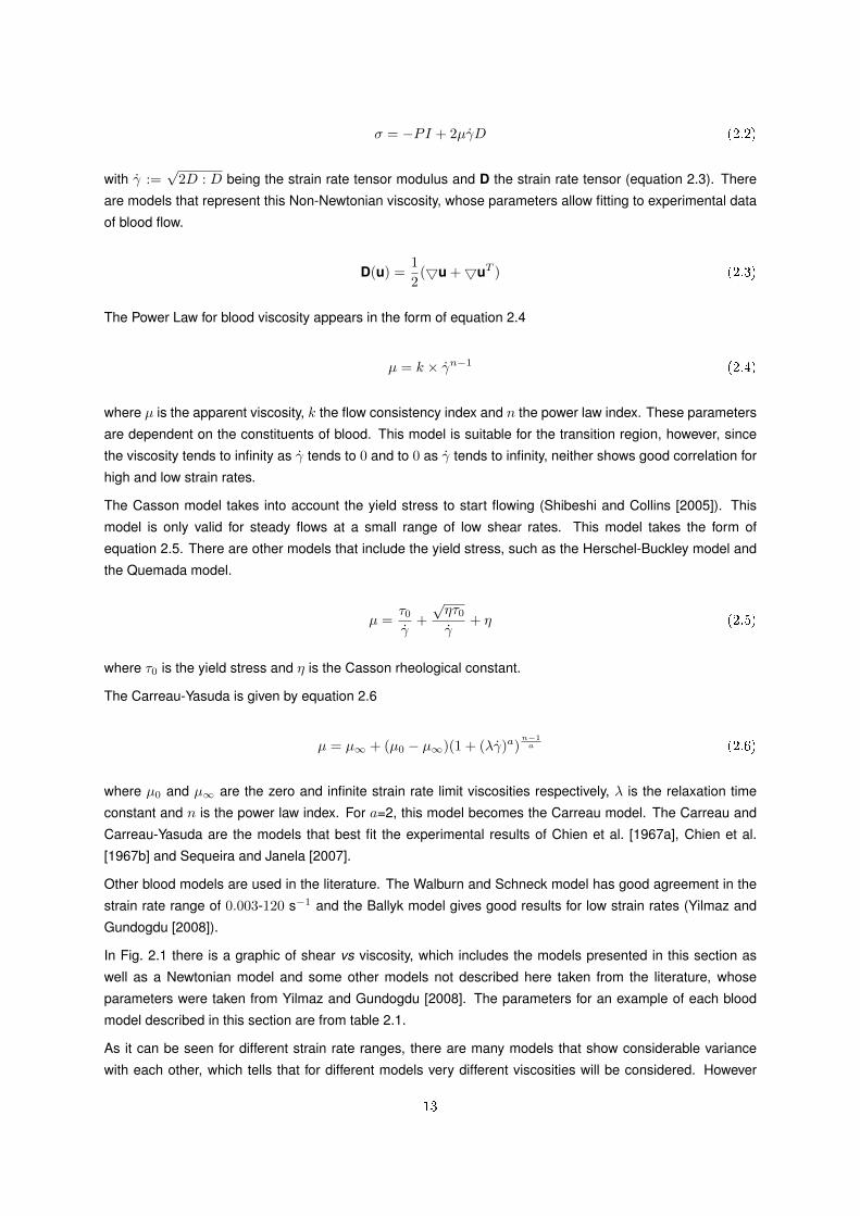
In Fig. 2.1 there is a graphic of shear vs viscosity, which includes the models presented in this section as

well as a Newtonian model and some other models not described here taken from the literature, whose

parameters were taken from Yilmaz and Gundogdu [2008]. The parameters for an example of each blood

model described in this section are from table 2.1.

As it can be seen for different strain rate ranges, there are many models that show considerable variance

with each other, which tells that for different models very different viscosities will be considered. However

13

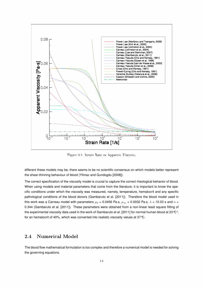
Figure 2.1: Strain Rate vs Apparent Viscosity

different these models may be, there seems to be no scientific consensus on which models better represent

the shear-thinning behaviour of blood (Yilmaz and Gundogdu [2008]).

The correct specification of the viscosity model is crucial to capture the correct rheological behavior of blood.

When using models and material parameters that come from the literature, it is important to know the spe-

cific conditions under which the viscosity was measured, namely, temperature, hematocrit and any specific

pathological conditions of the blood donors (Gambaruto et al. [2011]). Therefore the blood model used in

this work was a Carreau model with parameters µ0 = 0.0456 Pa.s, µ∞ = 0.0032 Pa.s, λ = 10.03 s and n =

0.344 (Gambaruto et al. [2011]). These parameters were obtained from a non-linear least square fitting of

the experimental viscosity data used in the work of Gambaruto et al. [2011] for normal human blood at 23°C°,

for an hematocrit of 40%, which was converted into realistic viscosity values at 37°C.

2.4 Numerical Model

The blood flow mathematical formulation is too complex and therefore a numerical model is needed for solving

the governing equations.

14

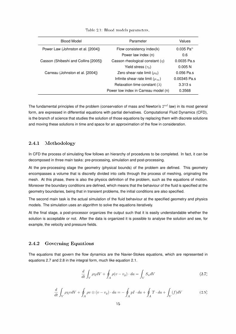
Table 2.1: Blood models parameters.

Blood Model Parameter Values

Power Law (Johnston et al. [2004]) Flow consistency index(k) 0.035 Pan

Power law index (n) 0.6

Casson (Shibeshi and Collins [2005]) Casson rheological constant (η) 0.0035 Pa.s

Yield stress (τ0) 0.005 N

Carreau (Johnston et al. [2004]) Zero shear rate limit (µ0) 0.056 Pa.s

Infinite shear rate limit (µ∞) 0.00345 Pa.s

Relaxation time constant (λ) 3.313 s

Power low index in Carreau model (n) 0.3568

The fundamental principles of the problem (conservation of mass and Newton’s 2nd law) in its most general

form, are expressed in differential equations with partial derivatives. Computational Fluid Dynamics (CFD),

is the branch of science that studies the solution of those equations by replacing them with discrete solutions

and moving these solutions in time and space for an approximation of the flow in consideration.

2.4.1 Methodology

In CFD the process of simulating flow follows an hierarchy of procedures to be completed. In fact, it can be

decomposed in three main tasks: pre-processing, simulation and post-processing.

At the pre-processing stage the geometry (physical bounds) of the problem are defined. This geometry

encompasses a volume that is discretly divided into cells through the process of meshing, originating the

mesh. At this phase, there is also the physics definition of the problem, such as the equations of motion.

Moreover the boundary conditions are defined, which means that the behaviour of the fluid is specified at the

geometry boundaries, being that in transient problems, the initial conditions are also specified.

The second main task is the actual simulation of the fluid behaviour at the specified geometry and physics

models. The simulation uses an algorithm to solve the equations iteratively.

At the final stage, a post-processor organizes the output such that it is easily understandable whether the

solution is acceptable or not. After the data is organized it is possible to analyse the solution and see, for

example, the velocity and pressure fields.

2.4.2 Governing Equations

The equations that govern the flow dynamics are the Navier-Stokes equations, which are represented in

equations 2.7 and 2.8 in the integral form, much like equation 2.1.

d

dt

∫V

ρχdV +

∮A

ρ(v − vg) · da =

∫V

SudV (2.7)

d

dt

∫V

ρχvdV +

∮A

ρv ⊗ (v − vg) · da = −∮A

pI · da+

∮A

T · da+

∫V

(f)dV (2.8)

15

The terms on the left-hand side of equation 2.8 are the transient term, which is null for steady-state flows,

and the convective flux. On the right-hand side are the pressure gradient term, the viscous flux and the body

force terms. T is the viscous stress tensor and the f term represents the external forces.

2.4.3 Spatial Discretization Methods

The just shown governing equations are to be replaced by approximate discrete formulae. In this section they

will be presented.

Finite Dierence Method

The finite difference method is one of the several techniques for approximating the solutions to differential

equations and is also used in calculating the face field values in the finite volume method. The formulae for

the finite differences can be obtained through the expansion in Taylor’s series.

As an example the finite difference equation of at a point (xi, yi) for a finite value of ∆x is to be approximated

by Taylor’s theorem:

φ(xi + ∆x, yi) = φ(xi, yi) +∂φ

∂x

∣∣∣∣i

∆x+∂2φ

∂x2

∣∣∣∣i

∆x2

2+∂3φ

∂x3

∣∣∣∣i

∆x3

3+ ... (2.9)

φ(xi + ∆x, yi) = φ(xi, yi)−∂φ

∂x

∣∣∣∣i

∆x+∂2φ

∂x2

∣∣∣∣i

∆x2

2− ∂3φ

∂x3

∣∣∣∣i

∆x3

3+ ... (2.10)

which can be algebraically manipulated into three different finite differences equations: central difference

(2.11), “upwind” (2.12) and progressive (2.13)

∂φ

∂x

∣∣∣∣i

=(φi+1,j − φi−1,j)

2∆xi+O

(∆x2,

∂3φ

∂x3

)(2.11)

∂φ

∂x

∣∣∣∣i

=(φi,j − φi−1,j)

∆xi+O

(∆x,

∂2φ

∂x2

)(2.12)

∂φ

∂x

∣∣∣∣i

=(φi+1,j − φi,j)

∆xi+O

(∆x,

∂2φ

∂x2

)(2.13)

These formulae show that there is an error induced by the truncation of the serie.

Analogously and considering more terms of the Taylor’s serie and hence more points, higher derivatives can

be obtained. The example was just for uniform meshes. When the mesh is non-uniform, for example if the

point xi+1 − xi = ∆x and xi − xi−1 = (1 + α)∆x, for φ′′i it yields in equation 2.14

φ′′i = 2

[φi+1

∆x(1 + α)(∆x(1 + α) + ∆x)− φi

∆x(1 + α)∆x+

φi−1

∆x(∆x(1 + α) + ∆x)

](2.14)

There are other ways of obtaining the finite difference equations such as polynomial interpolation and the

Padé approximation.

16

Finite Volume Method

The finite difference method approximates the solution of the derivatives in a point of the computational

domain, whose points were defined by a mesh, to a discrete finite difference equation. For the finite volume

method the discrete domain is divided into control volumes, Ω, surrounding each node point on a mesh. In

this method the differential equations are integrated in the control volume Ω, which contains a divergence

term, hence it is converted to a surface integral of the fluxes ~F ·~n by Gauss’s theorem.

∫ ∫ ∫Ω

div(~F )dΩ =

∫ ∫ ∫Ω

QdΩ (2.15)∫∂Ωj

~F · d~S =

∫∂Ωj

~F ·~ndS =

∫Ωj

dQ (2.16)

which in the discrete form is

Σ(~F ·~nS) = QjΩj (2.17)

where Σ refers to all the surfaces of the control volume Ωj .

Using the control volume method to find ∂Φ∂x yields in the following equations:

∫ ∫ ∫V

∂Φ

∂xdV = Φe~Se − Φw ~Sw (2.18)

= Φe∆y − Φw∆y (2.19)

=ΦE + ΦP

2∆y − ΦP + ΦW

2∆y (2.20)

=ΦE − ΦW

2∆y (2.21)

(2.22)

divided by the volume gives

∂Φ

∂x=

ΦE − ΦW2∆x

(2.23)

which is in fact the method used in the commercial code used in this Dissertation.

2.4.4 Meshing

As previously stated in the process of a CFD analysis the flow domain is split into smaller subdomains, which

are geometric primitives like polyhedrals or tetrahedrals. In many engineering applications the geometries

are complex. There are several ways of discretizing the geometry:

1. Structured meshes (either curvilinear orthogonal or non-orthogonal)

17

2. Non-Structured

The partial differential equations that govern fluid flow and heat transfer are not usually amenable to analytical

solutions, except for very simple cases. Therefore, in order to analyze fluid flows, flow domains are split into

smaller subdomains (made up of geometric primitives like hexahedra and tetrahedra in 3D and quadrilaterals

and triangles in 2D). The governing equations are then discretized and solved inside each of these subdo-

mains. Typically, one of three methods is used to solve the approximate version of the system of equations:

finite volumes, finite elements, or finite differences. Care must be taken to ensure proper continuity of solu-

tion across the common interfaces between two subdomains, so that the approximate solutions inside various

portions can be put together to give a complete picture of fluid flow in the entire domain. The subdomains are

often called elements or cells, and the collection of all elements or cells is called a mesh or grid. The origin

of the term mesh (or grid) goes back to early days of CFD when most analyses were 2D in nature. For 2D

analyses, a domain split into elements resembles a wire mesh, hence the name.

2.4.5 Boundary Conditions

In every CFD model, apart from the geometry definition and the consequent mesh, there is the need of

prescribing boundary conditions (section 2.4).

Blood flows by entering and exiting blood vessels, which have walls that do not allow for blood to pass through.

Therefore it is clear that for the inlet and outlet of the blood flow as well as for the walls there must be boundary

conditions. For the inlet a velocity inlet is used, being that an extrusion at the inlet is meshed, in order to have

fully-developed flow at the entrance of the portal vein. As for the outlets of the portal vein, knowing that the

pressure loss throughout the liver is about 600Pa and that the left part of the liver is approximately twice as

the right part, and therefore has a blood flow twice as high (Petkova [2008]), these flow exits were modeled

with pressure loss that is dependent on the velocity of the blood fluid through equation 2.24, where α is a

constant that is around twice as high in the right branch. The walls were modeled as being rigid and with a

no-slip condition, which means that they are impermeable and that the velocity is zero in the wall.

5 · p = −α~V (2.24)

2.4.6 Algorithms for the Solution of the Incompressible Conservation Equa-

tions

An algorithm for the solution of the conservation equations in primitive variables involves several options:

1. Equations and boundary conditions

2. Staggered or non-staggered meshes

3. Convection-diffusion discretization (several numerical schemes)

4. Velocity-pressure coupling (direct coupling, velocity-pressure correction, etc)

5. Solution of the algebraic equations system

18

In fact there are several families of calculation algorithms such as MAC, ICE, projection methods and SIMPLE,

which are used for different applications.

SIMPLE

SIMPLE is an acronym for Semi-Implicit Method for Pressure Linked Equations and was developed by

Patankar and Spalding [1972]. Today this algorithm is still used in a wide variety of commercial codes such

as Fluent ® and STAR-CCM+ ®, which is the code chosen and used in the simulations performed in this

Thesis. This algorithm obtains an approximated velocity field by solving the momentum equations and the

pressure gradient term is calculated using the pressure distribution from the previous iteration or an initial

guess, hence the name of this step, predictor step. The next step is the corrector step, where the mass resid-

ual Sm is calculated and the pressure equation is formulated and solved in order to obtain the new pressure

distribution (equations 2.25-2.28).

aP (ui)∗P =

∑f

af (u∗i · ni)f −1

ρ

δp

δxi

n

(2.25)

un+1 = u∗ + u′

pn+1 = p∗ + p′(2.26)

aP (ui)n+1P =

∑f af (un+1

i · ni)f − 1ρδpδxi

n+1

aP (ui)∗P =

∑f af (u∗i · ni)f − 1

ρδpδxi

n (2.27)

aP (ui)′P =

∑f

af[(un+1i − u∗i ) · ni

]f− 1

ρ

δp

δxi

′(2.28)

Then the velocity and pressure fields are corrected and a new set of conservative fluxes is calculated.

(ui)′P = (ui)

′ − 1

ap

1

ρ

δp′

δxi(2.29)

Pi,j = P ∗i,j + αPP′i,j (2.30)

This cycle is repeated until convergence is obtained, going back to the first step. A fluxogram of the SIMPLE

algorithm is presented in Fig. 2.2.

2.4.7 Star-CCM+®

Due to the complexity in implementing a CFD code, a commercial code was used for the simulations in this

dissertation, which was Star-CCM+®, a CD-Adapco® product. Star-CCM+® can be used to solve problems

involving flow, heat transfer and stress.

19

Figure 2.2: Fluxogram of the SIMPLE algorithm

This numerical solver has been tested and verified against several validated benchmark engineering prob-

lems. This product was also used throughout this work for mesh generation and CAD model handling.

Accurate numerical investigations of complex three-dimensional unsteady flows require the simultaneous

application of, at least, second-order discretization schemes applied on sufficiently refined meshes, and an

accurate representation of fluid rheology (Miranda et al. [2008]).

This numerical code uses a SIMPLE algorithm, and throughout this work a segregated flow model (solves

equations for velocity and pressure in a segregated or uncoupled manner) was chosen using a 2nd order

upwind convection scheme.

This way in this work, blood flow was modeled as a liquid, steady, laminar, three-dimensional with rigid walls,

constant density and Non-Newtonian viscous behaviour.

20

Chapter 3

Uncertainty Quantication Process

Uncertainty quantification is a process of characterization of uncertainties, determining the likelihood of a

certain outcome. As seen in previous chapters, there are some uncertainties regarding the blood flow in the

numerical model. In order to fully understand the influence of those uncertainties an uncertainty quantification

process is applied. This chapter is divided into two sections: the first section is an introduction to polynomial

chaos with the definition of stochastic process, orthogonal polynomials and the Askey-scheme, required for

the understanding of the non intrusive process; the second section describes the actual non intrusive process

used in this work to quantify the uncertainty in the portal vein. A more detailed description of the polynomial

chaos theory can be seen in the work of Xiu and Karniadakis [2002a].

3.1 Polynomial Chaos

The Polynomial Chaos (PC) expansion is a non-sampling based method that uses a spectral projection of the

random variables to determine the evolution of uncertainty in a dynamical system. The PC employs orthog-

onal polynomials in the random space as the trial basis to expand the stochastic process. The generalized

polynomial chaos expansion can handle several random processes, such as gaussian, beta, uniform, etc.

Certain distributions are associated with specific polynomials

A stochastic process has an intrinsically non-deterministic behaviour. The state of a stochastic process will

be determined by both predictable actions and random elements. The processes involve random variables,

which have non-deterministic quantities with a certain probability distribution.

A real-valued function (g) having a dependence in space (~x) and a random parameter (θ) with a known

Probability Density Function (PDF) is called a stochastic process and can be written as

g(~x, θ), ~x ∈ X , θ ∈ Θ (3.1)

Θ is called the support space of the random variable θ (Acharjee and Zabarras [2007]). This space is

characterized by a set of independent input random variables, which may have different distributions. The

21

resulting PDF of all random variables is given by equation 3.2.

f(ξ) =

N∏i=1

f(ξi) (3.2)

Orthogonal polynomials, which have the characteristic of having its inner product equal to zero (3.3), are

used in the PC expansion

〈φi, φj〉 =

∫φi.φjw(ξ)dξ = 0 , ∀i 6= j (3.3)

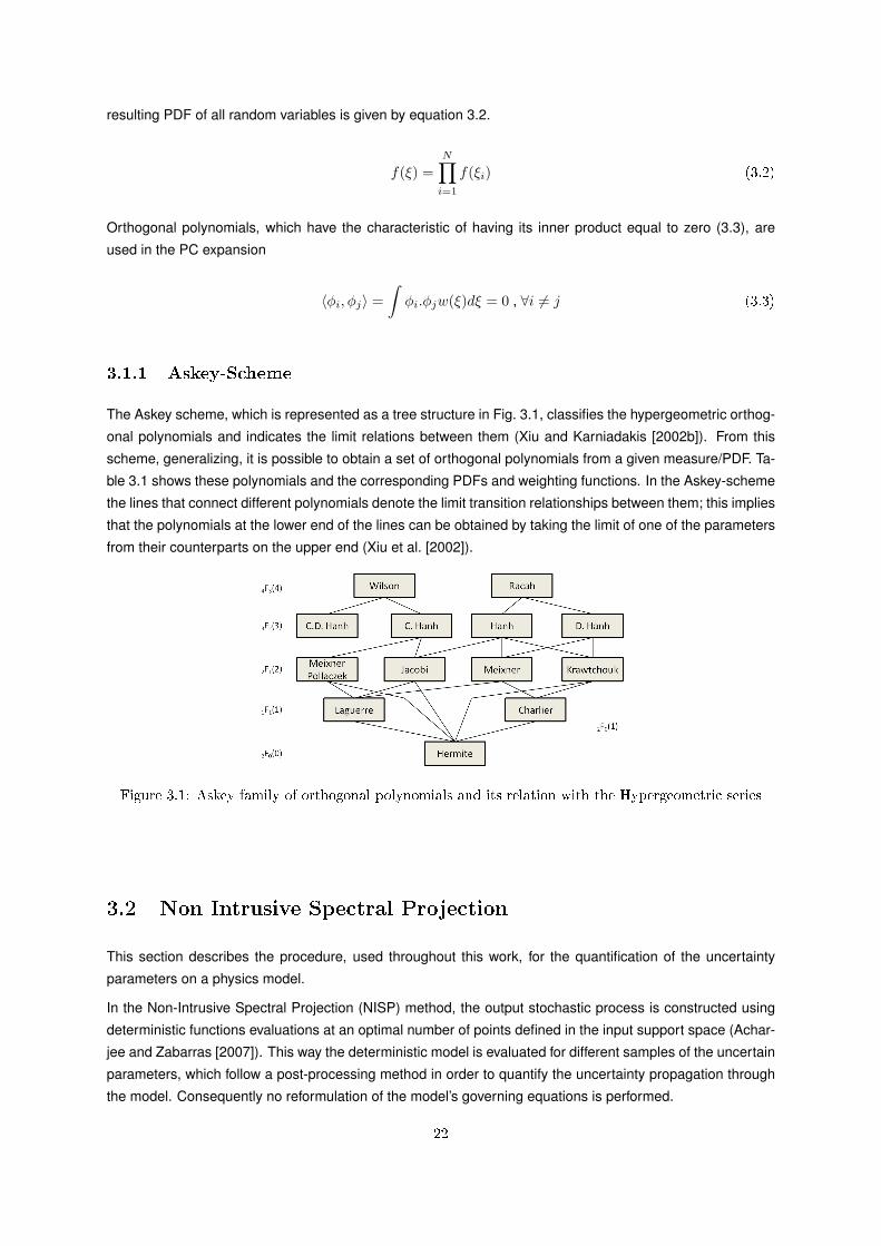
3.1.1 Askey-Scheme

The Askey scheme, which is represented as a tree structure in Fig. 3.1, classifies the hypergeometric orthog-

onal polynomials and indicates the limit relations between them (Xiu and Karniadakis [2002b]). From this

scheme, generalizing, it is possible to obtain a set of orthogonal polynomials from a given measure/PDF. Ta-

ble 3.1 shows these polynomials and the corresponding PDFs and weighting functions. In the Askey-scheme

the lines that connect different polynomials denote the limit transition relationships between them; this implies

that the polynomials at the lower end of the lines can be obtained by taking the limit of one of the parameters

from their counterparts on the upper end (Xiu et al. [2002]).

Figure 3.1: Askey family of orthogonal polynomials and its relation with the Hypergeometric series

3.2 Non Intrusive Spectral Projection

This section describes the procedure, used throughout this work, for the quantification of the uncertainty

parameters on a physics model.

In the Non-Intrusive Spectral Projection (NISP) method, the output stochastic process is constructed using

deterministic functions evaluations at an optimal number of points defined in the input support space (Achar-

jee and Zabarras [2007]). This way the deterministic model is evaluated for different samples of the uncertain

parameters, which follow a post-processing method in order to quantify the uncertainty propagation through

the model. Consequently no reformulation of the model’s governing equations is performed.

22

Table 3.1: Orthogonal polynomials of the Askey family and theirrespective weighting functions .

Polynomials Weighting Function PDF

Hermite H(x) e−ξ2

2 Gaussian

Laguerre L(x) xαe−x Gamma

Jacobi P (x) (1− x)α(1 + x)β Beta/Uniform

Charlier C(x) ax

x! Poisson

Krawtchouk Kn(x)

(N

x

)px(1− p)N−x Binomial

Meixner Mn(x) (β)xx! (1− c)βcx Negative Binomial

Hahn Qn(x)

(α+ x

x

)(β +N − xN − x

)Hypergeometric

Let X be a model uncertain parameter and f a corresponding solution variable. In general, for a prescribed

PDF of X, X(ξ) can be represented using a PC expansion given by equation 3.4

X(ξ) =

p∑j=0

cXn In(ξ) (3.4)

Following the Askey scheme described in section 3.1.1, depending on the PDF of the random variable ξ

different orthogonal polynomials In are used to minimize the PC expansion (see table 3.1). Table 3.2 resumes

some information about Hermite, Jacobi and Legendre uni-dimensional polynomial sets that are associated

with a Normal, Beta and Uniform distributed random variable ξ , respectively.

Table 3.2: Main information for Hermite, Jacobi and Legendre unidimensional polynomial sets.

Property Hermite Jacobi Legendre

Orthogonality interval ]−∞,+∞[ [−1, 1] [a, b]

PDF of ξ Normal (0,1) Beta (-1,1;α,β) α, β ≥ −1 Uniform (a,b) −∞ < a < b < +∞Mean value µξ 0 β−α

α+β+2a+b

2

Variance σ2ξ 1 4(α−1)(β−1)

(α+β+2)2(α+β+3)b−a12

Weight, w(ξ) e−(ξ−µ)2

2σ2√2πσ2

(1−ξ)α(1+ξ)β

〈I20〉

1b−a a ≤ ξ ≤ b0 ξ < a ∪ ξ > b.

This method can be generalized forN independent random variables (X1, ...XN ). For each variable there will

be an associated stochastic dimension ξi=1, ..., N , which forms a multi-dimension stochastic space, whose

orthogonality polynomials are given in the form of equation 3.5

f(n) =

I0,

I1(ξi) , i = 1, ..., N

I2(ξi, ξj) , i = 1, ..., N ; j ≤ i

I3(ξi, ξj , ξk) , i = 1, ..., N ; k ≤ j ≤ i

...

(3.5)

23

where ~ξ = (ξ1, ..., ξN ) is the random variables vector. The orthogonal polynomials In(~ξ) are obtained from

the tensor products. The orthogonality is given in the form of equation 3.6 and the polynomials are usually

renumbered with only one index as Φj .

〈Φi,Φj〉 =

∫ΦiΦjw(~ξ)dξ =

⟨Φ2j

⟩δij (3.6)

Having the orthogonal polynomials, the model solution f(~ξ) can be represented using the PC expansion

f(~ξ) =

P∑j=0

cfjΦj(~ξ) (3.7)

where cfj are the unknown PC expansion mode coefficients of f(~ξ) and P + 1 = (N + p)!/(N !p!) the total

number of terms in the PC expansion, with p equal to the maximum polynomial order of the expansion. Thus

given the orthogonality of Φj , cfj yields in:

cfj =

⟨f(~ξ)Φj

⟩⟨Φ2j

⟩ , j = 0, ..., P (3.8)

The above formulation for the uncertainty parameters and field variables has been used for an intrusive spec-

tral projection approach, where the reformulated governing equations are solved to determine the coefficients

cfj very effectively. However this method requires the recoding of the numerical source code, which is im-

practical for the flow problem solution in this work. The NISP method surges as an alternative for using the

deterministic solutions fd for different values of the uncertainty parameters.

In general the NISP method is developped through the following process (Mendes [2010] and Reagan et al.

[2003]).

1. Define the PDFs for the uncertainty parameters Xi, i = 1, ..., N , thus associating the distribution type

with the PC basis Φj . The random variables vector (~ξ) is determined using a procedure described in

detail in the work of Mendes [2010].

2. Determine the corresponding spectral PC expansion for each of the parameters using equation 3.4.

3. Run the deterministic model for all the samples of the input parameters vector, (X1, ..., XN )nsn=1, to

obtain the solution for (fd)nsn=1

4. Evaluate the expectations from equation 3.8 over a sufficiently large number of samples to obtain the

solution for the spectral coefficients cfj . The numerator in equation 3.8 is solved numerically using a

Gauss quadrature (Appendix B), and whose solution is given by equation 3.9

cff ≈∑S1,...,SNr1,...,rN=1 fd(Xr1 , ..., XrN )Φj(ξr1 , ..., ξrN )

∏Ni=1 qri⟨

Φ2j

⟩ , k = 0, ..., P (3.9)

where (ξri , qri), r = 1, ...Si are the Gauss quadrature points and corresponding weights sampled on

the random variable ξi, ∀i ∈ 1, ..., N .

24

When all the information of the deterministic solutions is gathered, there are stochastic parameters that can

be taken about the model solution, such as the mean value f and the variance σ2f of the stochastic solution

f(~ξ) through equations 3.10 and 3.11.

f =< f >= cf0 (3.10)

σ2f =< f2 > − < f >=

P∑k=1

(cfk)2 < Φ2k > (3.11)

For the PDF and CDF of each stochastic solution variable, an approximation is done by employing a Kernel

Density Estimation technique, which is described in the work of Mendes [2010].

25

Chapter 4

Verication and Validation

Being the study of blood flow in the cardiovascular system a very difficult situation to reproduce in a laboratory,

the numerical cannot be quantitatively compared with an actual situation of blood flow in the human body.

However, there have been authors who have tried to replicate this physical phenomenon and whose results

are accepted as accurate in the scientific community Chen et al. [2006] and Bertolotti and Deplano [2000]).

In this Chapter, the verification of the numerical model is made with a semi-analytical benchmark case and

the validation to a real model is performed by comparing results with a recognized work in blood flow.

4.1 Verication

A Model verification is the substantiation that a computerized model represents a conceptual model within

specified limits of accuracy (Oberkampf and Trucano [2002]).

4.1.1 Methods

Following the work of Janela et al. [2010], the verification of the numerical solver was performed through the

study of blood flow inside a cylindrical duct with steady laminar fully developed flow (Figs. 4.1 and 4.2).

Since the pressure gradient must be constant5p =(

0, 0, ∂p∂x

)and the shear rate is given by γ =

∣∣∂Ux∂r

∣∣, the

Navier-Stokes equations can be written, in cylindrical coordinates (r, θ, x) as follows:

DUxDt

≡ 0⇔

⇔ 0 = −∂p∂x

+1

r

∂

∂r

(µr∂Ux∂r

)⇔

⇔ ∂p

∂x

r2

2= µr

∂Ux∂r

27

Figure 4.1: Cylindrical Duct Figure 4.2: Velocity eld in the XY plane

and since

µ = µ

(∂Ux∂r

)(4.1)

the velocity field can be derived into an implicit ordinary differential equation 4.2

∂Ux∂r

=∂p

∂x

r

2µ(∂Ux∂r

) (4.2)

where µ is given by a Carreau model in equation 4.3

µ = µ∞ + (µ0 − µ∞)(1 + (λγ)2)n−12 (4.3)

This equation does not have an explicit solution, therefore a numerical method is used to obtain ∂Ux∂r and

then by equation 4.4 the velocity profile is obtained. The values used for the Carreau model were µ∞ = 0.035

Pa.s, µ0 = 0.56 Pa.s, λ = 3.313 s and n = 0.334.

Ux(r) =

∫ R

r

∂Ux∂r

(s)ds (4.4)

This integration is also done numerically, and that is why the solution is semi-analytical. For the numerical

values of the semi-analytical solution a very accurate integration quadrature has been used.

For the CFD simulation a specified mass flow rate (4.279 × 10−3kg/s) was imposed in the cylindrical duct,

being the outlet periodic with inlet to simulate fully developed conditions.

For comparison purposes, a Newtonian model was also used with µ =const= 0.0035 Pa.s. For Newtonian

fluids the solution for fully-developed flow inside a cylindrical duct is analytical (Poiseuille Flow) and the

velocity in cylindrical coordinates only as an axial component, dependent on the radius, and is given by

equation 4.5.

v(r) =1

4µ

∂P

∂x

(R2 − r2

)(4.5)

where

28

∂P

∂x= 8Qµ

(ρπR4

)(4.6)

4.1.2 Results

As it was expected the velocity is constant along the axial coordinate. The shape of the velocity profile both

for the Newtonian and Non-Newtonian fluids can be seen in Fig. 4.3. The Newtonian fluid shows a parabolic

profile as its analytical equation suggests, whereas the Carreau model shows a blunter profile, which is due to

the fact that ∂Ux∂r is lower in the Non-Newtonian fluid than the Newtonian due to an higher apparent viscosity.

Figure 4.3: Velocity proles of the Newtonian and Non-Newtonian ows

Bearing in mind that the numerical solution is dependent on the size of the mesh and scheme used, a

convergence study with mesh refinement was performed for two types of meshes: polyhedral and trimmed.

Also in order to verify the actual order of the scheme used, both a 2nd and 1st order schemes where used for

different mesh sizes. In table 4.1 the size of the mesh, the scheme used and the absolute error of the axial

velocity are shown. The absolute error was calculated from equation 4.7.

||ε||2 =

√√√√∑Nj=1(Vex − Vnum)2 × V ol∑N

i=1 V ol(4.7)

It can be seen from Fig. 4.4 that all the solutions for the Non-Newtonian velocity profile are very close to the

semi-analytical solution. However looking closer in Fig. 4.5 it can be seen that there are some differences

and that as the mesh gets more refined the solution gets closer to the semi-analytical solution.

The convergence of the mesh is best seen in Fig. 4.6, where the error of the simulations mentioned in

Table 4.1 is plotted in a log-log scale. A first order slope is also ploted in order to be easy to compare. As

it can be seen as the mesh get more refined the slope decreases into an order inferior than the first. This

situation is explained by the fact that error is already stabilizing and that for non-orthogonal meshes the CFD

commercial code does not give 2nd order solutions. To confirm this a simpler model was run in a 2D duct,

29

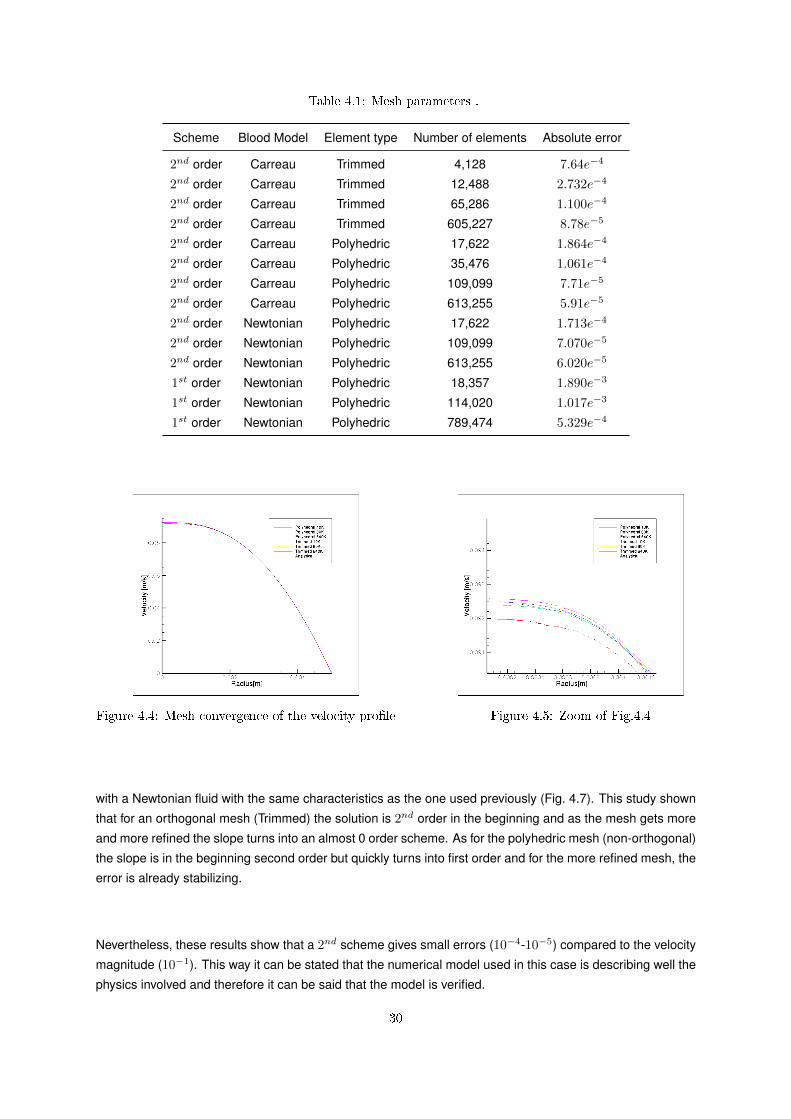
Table 4.1: Mesh parameters .

Scheme Blood Model Element type Number of elements Absolute error

2nd order Carreau Trimmed 4,128 7.64e−4




2nd order Carreau Polyhedric 17,622 1.864e−4




2nd order Newtonian Polyhedric 17,622 1.713e−4



1st order Newtonian Polyhedric 18,357 1.890e−3



Figure 4.4: Mesh convergence of the velocity prole Figure 4.5: Zoom of Fig.4.4

with a Newtonian fluid with the same characteristics as the one used previously (Fig. 4.7). This study shown

that for an orthogonal mesh (Trimmed) the solution is 2nd order in the beginning and as the mesh gets more

and more refined the slope turns into an almost 0 order scheme. As for the polyhedric mesh (non-orthogonal)

the slope is in the beginning second order but quickly turns into first order and for the more refined mesh, the

error is already stabilizing.

Nevertheless, these results show that a 2nd scheme gives small errors (10−4-10−5) compared to the velocity

magnitude (10−1). This way it can be stated that the numerical model used in this case is describing well the

physics involved and therefore it can be said that the model is verified.

30

Figure 4.6: Mesh Convergence in Log scale for a 3D cylindrical duct: PNN 2nd - Polyhedric mesh,Non-Newtonian, 2nd order scheme; TNN 2nd - Trimmed mesh , Non-Newtonian, 2nd order scheme; PN2nd - Polyhedric mesh, Newtonian, 2nd order scheme PN 1st - Polyhedric mesh, Newtonian, 1st orderscheme 1st - real 1st order scheme

4.2 Validation

A model validation is the substantiation that a computerized model within its domain of applicability pos-

sesses a satisfactory range of accuracy consistent with the intended application of the model (Oberkampf

and Trucano [2002]). In order to fulfill this requirement the work of Chen et al. [2006] and Bertolotti and De-

plano [2000] was reproduced. Even though the articles in question do not represent the actual flow of blood

in the human body, they are highly dignified articles in the extent of blood rheology, being cited in several

articles of this field. Therefore these were considered as valid for the validation of the numerical model used

throughout this work.

4.2.1 Methods

The assumption of Newtonian behaviour of blood is acceptable for high shear rate flow, e.g. in the case of

flow through large arteries. It is not, however, valid when the shear rate is low (0.1-100 s−1) which is the case

in small arteries and in the downstream side of the stenosis. The Non-Newtonian character of blood is typical

in small arteries and veins where the presence of the cells induces that specific behaviour (Tu and Deville

[1996]).

In the study of Chen et al. [2006], steady Non-Newtonian flow in a simplified geometry for coronary bypass

is simulated under different flow conditions and graft locations (Chen et al. [2006]). The 3D Navier–Stokes

equations coupled with the Non- Newtonian constitutive model are solved numerically using a finite element

method (Chen et al. [2006]).

The geometry used in the modeling of the simulation can be seen in Fig 4.8, where a simplified anastomosis

model is represented as the intersection of two cylinders both with a diameter of D = 3 mm (Ofili et al. [1995])

at a junction angle of 45. A 75% lumen axisymmetric stenosis is considered in the host coronary and is

described by a Gaussian profile (Siouffi et al. [1998]) given by equation 4.8, where R(x) is the radius of the

31

Figure 4.7: Mesh Convergence in Log scale for a 2D cylindrical duct

Figure 4.8: Graft Geometry

constricted part in the host coronary withR0 = 1.5 mm and xs = -6 mm represents the position of the stenosis.

R(x)

R0= 1− 1

2exp

(−4(x− xs)2

R02

)(4.8)

The blood flow was modeled as being incompressible, Non-Newtonian, homogeneous, steady, three-dimensional

and laminar. The shear thinning behaviour, the most dominant Non-Newtonian property of blood, was mod-

eled with a Carreau-Yasuda model (equation 2.6) with µ∞ = 0.0022 Pa.s, µ0 = 0.022 Pa.s, λ = 0.110 s, a =

0.644 and n = 0.392 and the blood density is considered to be ρ = 1410 kg/m3. For the inlet of the host artery

and graft, the boundary conditions are mass flow rate inlets of 34Q and 3

4Q respectively with Q = 1.708×10−3

kg/s. Also at the inlet of both cylinders, an inlet extrusion is originated, in order to get fully developed flow at

those surfaces. For the host artery outlet an extrusion is also generated to allow for a traction-free boundary.

32

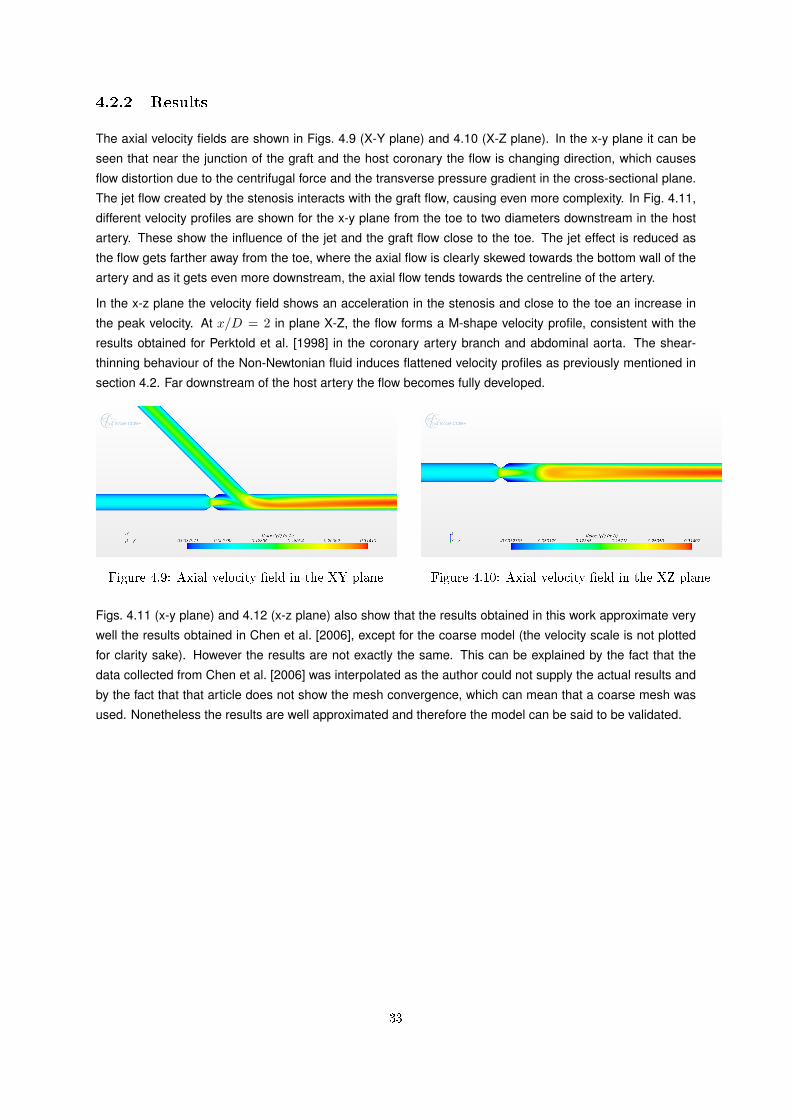
4.2.2 Results

The axial velocity fields are shown in Figs. 4.9 (X-Y plane) and 4.10 (X-Z plane). In the x-y plane it can be

seen that near the junction of the graft and the host coronary the flow is changing direction, which causes

flow distortion due to the centrifugal force and the transverse pressure gradient in the cross-sectional plane.

The jet flow created by the stenosis interacts with the graft flow, causing even more complexity. In Fig. 4.11,

different velocity profiles are shown for the x-y plane from the toe to two diameters downstream in the host

artery. These show the influence of the jet and the graft flow close to the toe. The jet effect is reduced as

the flow gets farther away from the toe, where the axial flow is clearly skewed towards the bottom wall of the

artery and as it gets even more downstream, the axial flow tends towards the centreline of the artery.

In the x-z plane the velocity field shows an acceleration in the stenosis and close to the toe an increase in

the peak velocity. At x/D = 2 in plane X-Z, the flow forms a M-shape velocity profile, consistent with the

results obtained for Perktold et al. [1998] in the coronary artery branch and abdominal aorta. The shear-

thinning behaviour of the Non-Newtonian fluid induces flattened velocity profiles as previously mentioned in

section 4.2. Far downstream of the host artery the flow becomes fully developed.

Figure 4.9: Axial velocity eld in the XY plane Figure 4.10: Axial velocity eld in the XZ plane

Figs. 4.11 (x-y plane) and 4.12 (x-z plane) also show that the results obtained in this work approximate very

well the results obtained in Chen et al. [2006], except for the coarse model (the velocity scale is not plotted

for clarity sake). However the results are not exactly the same. This can be explained by the fact that the

data collected from Chen et al. [2006] was interpolated as the author could not supply the actual results and

by the fact that that article does not show the mesh convergence, which can mean that a coarse mesh was

used. Nonetheless the results are well approximated and therefore the model can be said to be validated.

33

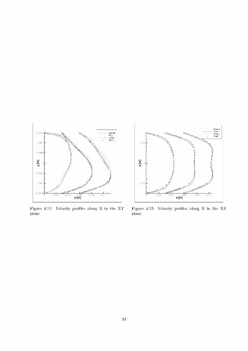
Figure 4.11: Velocity proles along X in the XYplane

Figure 4.12: Velocity proles along X in the XZplane

34

Chapter 5

Results

This Chapter describes the propagation of parametric uncertainty through a physical model, which is used to

investigate the problem concerning blood flow in the portal vein for people with liver cirrhosis. The uncertainty

quantification problem is addressed using a NISP based method, which allows one to obtain the stochastic

solution using the original deterministic model without requiring modifications in the source code (Mendes

[2010]). The uncertainty parameters studied were based on the uncertainty on blood viscosity models and

on the range of precision of MRI’s on the model’s geometry. This Chapter shows firstly the deterministic

models with a convergence study, as well as the geometry definition for a Newtonian and Non-Newtonian

model, following a description and source of the parametric uncertainties with the results obtained using the

NISP method for both the blood and geometry uncertainties.

5.1 Deterministic Model

5.1.1 Geometry and Convergence Analysis

The portal vein model is described by a main vein that branches into two, and those two branches into four

different ones. The model used for the portal vein has the dimensions given in Table 5.1. Since the purpose

of this work was to simulate a disease portal vein, a clot was included in the geometry to simulate thrombosis

in the portal vein. This clot was modeled as a cylindrical cut through the model’s left branch. The clot as well

as the whole portal vein geometry can be seen in Fig. 5.1.

Bearing in mind the verification and validation study already performed, a few meshes were simulated in order

to find if the model was converged. The convergence analysis was performed using a velocity profile from

the left branch straight after the clot in different meshes. Fig. 5.2 shows five different profiles with different

number of elements in the mesh. Assuming that the more refined model (5.418M elements) is the closest to

the right solution, the mesh with 3.189M elements shows a very good fitting in the velocity profile showing it

is well converged, therefore this mesh was the one chosen throughout the rest of the work.

35

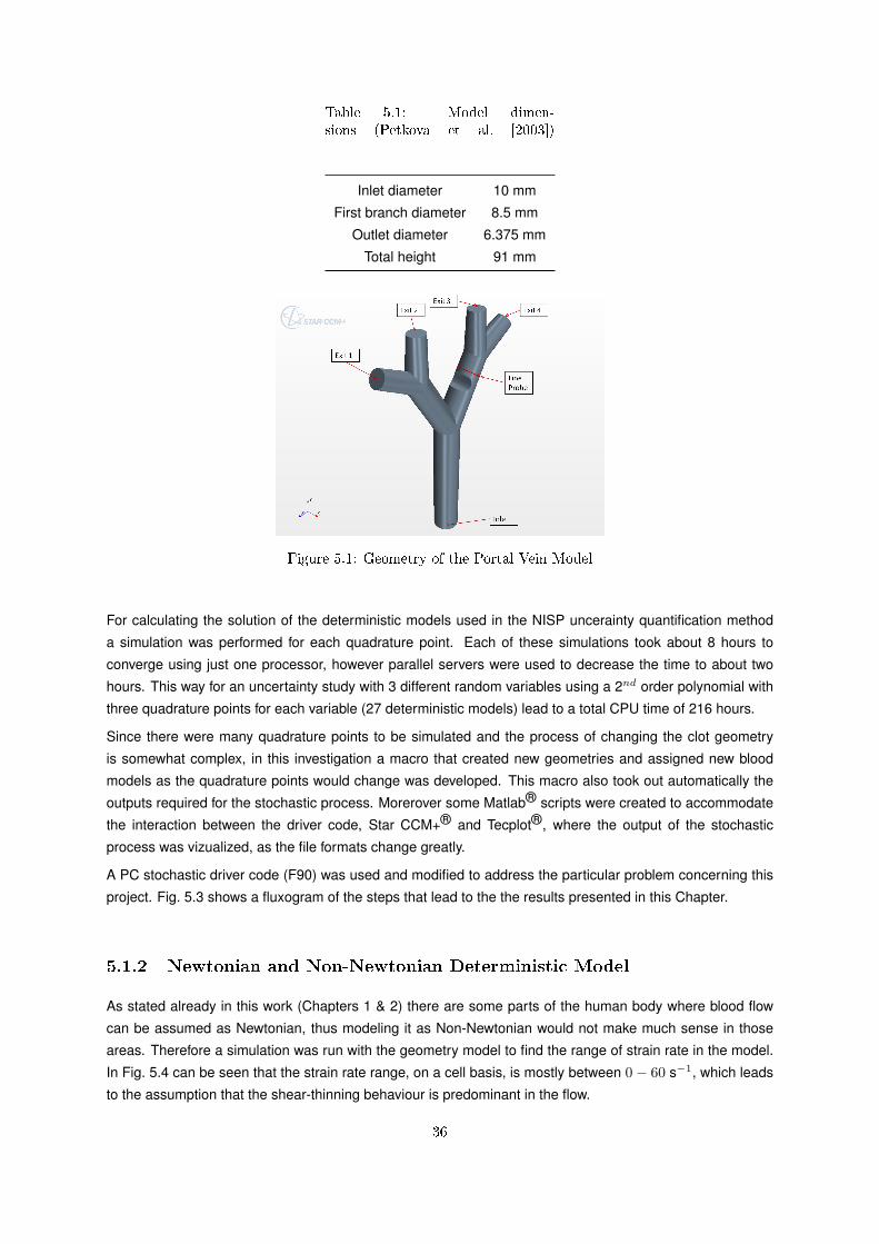
Table 5.1: Model dimen-sions (Petkova et al. [2003])

Inlet diameter 10 mm

First branch diameter 8.5 mm

Outlet diameter 6.375 mm

Total height 91 mm

Figure 5.1: Geometry of the Portal Vein Model

For calculating the solution of the deterministic models used in the NISP uncerainty quantification method

a simulation was performed for each quadrature point. Each of these simulations took about 8 hours to

converge using just one processor, however parallel servers were used to decrease the time to about two

hours. This way for an uncertainty study with 3 different random variables using a 2nd order polynomial with

three quadrature points for each variable (27 deterministic models) lead to a total CPU time of 216 hours.

Since there were many quadrature points to be simulated and the process of changing the clot geometry

is somewhat complex, in this investigation a macro that created new geometries and assigned new blood

models as the quadrature points would change was developed. This macro also took out automatically the

outputs required for the stochastic process. Morerover some Matlab® scripts were created to accommodate

the interaction between the driver code, Star CCM+® and Tecplot®, where the output of the stochastic

process was vizualized, as the file formats change greatly.

A PC stochastic driver code (F90) was used and modified to address the particular problem concerning this

project. Fig. 5.3 shows a fluxogram of the steps that lead to the the results presented in this Chapter.

5.1.2 Newtonian and Non-Newtonian Deterministic Model

As stated already in this work (Chapters 1 & 2) there are some parts of the human body where blood flow

can be assumed as Newtonian, thus modeling it as Non-Newtonian would not make much sense in those

areas. Therefore a simulation was run with the geometry model to find the range of strain rate in the model.

In Fig. 5.4 can be seen that the strain rate range, on a cell basis, is mostly between 0− 60 s−1, which leads

to the assumption that the shear-thinning behaviour is predominant in the flow.

36

Figure 5.2: Convergence Graphic of a Velocity prole in the left branch after the clot for dierent sizedmeshes

To verify that, in fact, in this model the shear-thinning behaviour is important two models were simulated

with Newtonian and Non-Newtonian behaviour. The Newtonian model used a constant viscosity of µ =

0.0035Pa.s, whereas the Non-Newtonian used a Carreau model for the fluid viscosity with parameters µ0 =

0.0456Pa.s, µ∞ = 0.0032Pa.s and n = 0.344. The radius of the clot was constant and equal to 2.833 mm.

In Fig. 5.5 is plotted the absolute difference in the velocity magnitude throughout the models, being possible

to see the velocity field in Fig. 5.6 for Non-Newtonian flow. From this it can be seen that mostly in the right

branch the differences are larger. However, if we consider the relative difference, taking into consideration

the two figures, there are also significant differences in the recirculation zone, which is a very important factor

in blood flow, due to the fact that if a recirculation bubble persists for a long time, the slowed RBCs will

aggregate(Chapter 1) increasing the chances of increasing the blood clot.

5.2 Stochastic Inuence of the Thrombosis Radius

Having decided on which viscosity model was to be implemented, the introduction of uncertainty parameters

in the model’s geometry follows. In this section the radius of the thrombosis in the model’s left branch was

taken as a random variable.

5.2.1 Small Obstruction

The size of the thrombosis has a great influence in the hemodynamic characteristics of the flow, specially

in the wall shear stress. Adding to this, the fact that current MRI tools only have a limited accuracy, which

varies from 0.3mm (Milner et al. [1998]), 0.06-0.47mm (Hammer et al. [2009]) and 0.4mm (Gambaruto et al.

[2011]) shows that care must be taken when analyzing small arteries or veins. Thus the fact that MRI exams

are performed in awaken subjects, which can move during the exam adds more uncertainty to the actual size

37

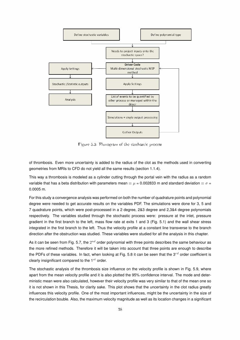
Figure 5.3: Fluxogram of the stochastic process

of thrombosis. Even more uncertainty is added to the radius of the clot as the methods used in converting

geometries from MRIs to CFD do not yield all the same results (section 1.1.4).

This way a thrombosis is modeled as a cylinder cutting through the portal vein with the radius as a random

variable that has a beta distribution with parameters mean ≡ µ = 0.002833 m and standard deviation ≡ σ =

0.0005 m.

For this study a convergence analysis was performed on both the number of quadrature points and polynomial

degree were needed to get accurate results on the variables PDF. The simulations were done for 3, 5 and

7 quadrature points, which were post-processed in a 2 degree, 2&3 degree and 2,3&4 degree polynomials

respectively. The variables studied through the stochastic process were: pressure at the inlet, pressure

gradient in the first branch to the left, mass flow rate at exits 1 and 3 (Fig. 5.1) and the wall shear stress

integrated in the first branch to the left. Thus the velocity profile at a constant line transverse to the branch

direction after the obstruction was studied. These variables were studied for all the analysis in this chapter.

As it can be seen from Fig. 5.7, the 2nd order polynomial with three points describes the same behaviour as

the more refined methods. Therefore it will be taken into account that three points are enough to describe

the PDFs of these variables. In fact, when looking at Fig. 5.8 it can be seen that the 3rd order coefficient is

clearly insignificant compared to the 1st order.

The stochastic analysis of the thrombosis size influence on the velocity profile is shown in Fig. 5.9, where

apart from the mean velocity profile and it is also plotted the 95% confidence interval. The mode and deter-

ministic mean were also calculated, however their velocity profile was very similar to that of the mean one so

it is not shown in this Thesis, for clarity sake. This plot shows that the uncertainty in the clot radius greatly

influences this velocity profile. One of the most important influences, might be the uncertainty in the size of

the recirculation bouble. Also, the maximum velocity magnitude as well as its location changes in a significant

38

Figure 5.4: Bar Chart of the Strain Rate values in the model

Figure 5.5: Absolute dierence of the velocity eld-between a Newtonian and a Non-Newtonian bloodmodel

Figure 5.6: Velocity eld of the Non-Newtonianblood model

39

manner, which is caused by the change in the size of the recirculation buble. The mean velocity profile shows

an even distance between the confidence interval, apart from the recirculation buble and the middle of the

velocity profile, where it is closer to the lower and upper limits of the confidence interval, respectively.

The scalar values measured show different influences in the flow with the shear being highly influenced with

large standard deviation and the pressure inlet showing little influence. However, when comparing the shape

of both PDF (Figs. 5.7 and 5.10), it is clear that they are similar.

In Table 5.2 it is possible to check the mean and standard deviation values for other flow properties measured

(exit 1, exit 3 and pressure gradient in the left branch). Clearly from the values of the standard deviation

compared with the mean values of both mass flows measured, the flow split is almost unaltered by the

uncertainty in a small obstruction.

When looking at Figs. 5.11 and 5.12 it can be seen that the velocity is mostly affected by the radius uncertainty

close to the clot. The velocity values around the clot are were interpolated in a clot free model to accomodate

the PDF’s entire range.

Table 5.2: Mean and standard deviation values with theradius as a random variable.

Studied Mean Value Standard

Parameters µ deviation σ.

Shear[N] 0.201 ∗ 10−3 0.111 ∗ 10−4

Pressure Gradient[Pa] 0.482 ∗ 101 0.108 ∗ 101

Pressure Inlet[Pa] 0.672 ∗ 103 0.557 ∗ 100

Mass flow at exit 1[kg/s] 0.9917 ∗ 10−3 0.8819 ∗ 10−6


Figure 5.7: PDF for the Shear with the radius as a random variable

40

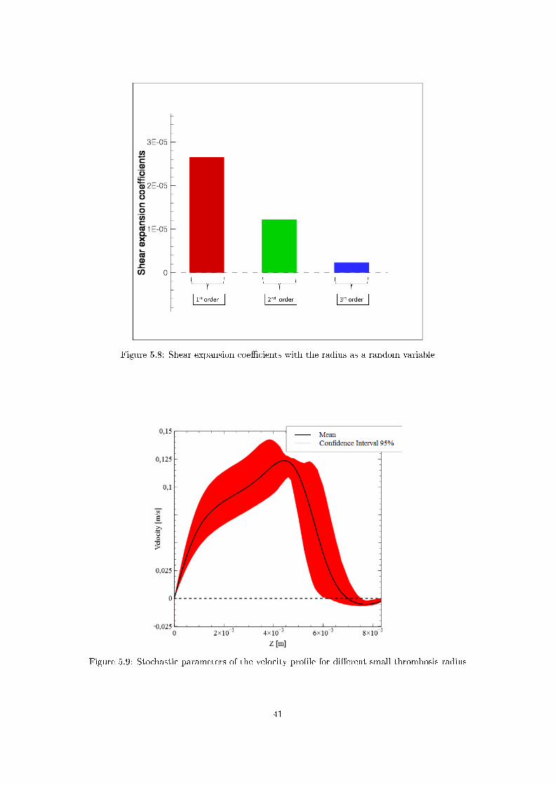
Figure 5.8: Shear expansion coecients with the radius as a random variable

Figure 5.9: Stochastic parameters of the velocity prole for dierent small thrombosis radius

41

Figure 5.10: PDF for the Pressure at the inlet with the thrombosis with the radius as a random variable

Figure 5.11: Average of the velocity eld with theradius as a random variable

Figure 5.12: Standard deviation of the velocity eldwith the radius as a random variable

42

5.2.2 Critical Radius

For large obstructions human life becomes at a great risk. When considering an obstruction of about 70%

of the vein diameter, the sensitivity of the MRI becomes even more critical as a small change in the size

of the thrombosis can lead to even greater changes in the hemodynamic factors. Therefore a study was

performed to analyse the influence of the geometry uncertainty in a critical thrombus with µ = 0.00595 m and

σ = 0.0005 m, which is the same standard deviation as previously used, since it is supposed to simulate the

MRI’s resolution uncerainty.

As expected the geometry uncertainty in the bigger clot has bigger influence in the flow inside the vein. This is

shown mostly by the confidence interval of the velocity profile (Fig. 5.13), clearly showing a large uncertainty

regarding the maximum velocity in that zone. Also the recirculation zone is longer, which will increase the

“roulleaux” formation and therefore increasing the chances of a larger and possibly deathly clot. Since now

the clot is so large that the line probe used for the velocity profile was inside the clot, it was taken a little

farther away from the clot keeping the same distance from the clot as before.

The large increase in not only the shear range, but also in its magnitude suggests an increased probability

of vein rupture leading to death. Leading to this increase in shear is the fact that the pressure at the inlet

has also vastly increased and with larger standard deviation. These behaviours can be seen in Figs. 5.14

and 5.15.

From Table 5.3 it is now possible to see that the mass flow split is affected by the uncertainty in the large

obstruction, whereas in the small clot it almost did not have any influence.

Figure 5.13: Stochastic parameters of the velocity prole for dierent thrombosis radius

43

Figure 5.14: PDF for the Shear with the radius as a random variable

Figure 5.15: PDF for the Pressure at the inlet with the thrombosis with the radius as a random variable

Table 5.3: Mean and standard deviation values with theradius as a random variable.



Shear[N] 0.768 ∗ 10−3 0.174 ∗ 10−3





44

5.3 Stochastic Inuence of the Blood Viscosity

This section shows the influence of the uncertainty regarding the blood viscosity. This uncertainty was mea-

sured using three different methods: uncertainty in the blood behaviour regarding a mixture of blood models;

uncertainty regarding the parameters in a Carreau blood viscosity model; uncertainty in the which distinctive

blood model describes blood viscosity.

5.3.1 Model Uncertainty

From section 2.3, comes the question of which is the blood viscosity model that will best describe the blood

flow in the portal vein case. As this question remains unanswered, it is important to take into account this

unknown into a stochastic process. Since the Carreau and Carreau-Yasuda is vastly used throughout the

literature (Shibeshi and Collins [2005], Gambaruto et al. [2011], Chen et al. [2006], etc.), it will be assumed

that the blood viscosity distribution with strain rate assumes such behaviour. In order to quantify the uncer-

tainty of these blood models, a function of the blood viscosity is used in the form of equation 5.1, where

φj(ξ, η) is a shape function that has values between [0, 1] and∑4j=1 φj(ξ, η) = 1. ξ and η are two ran-

dom variables with an uniform PDF varying in the range of [−1, 1]. Three different Carreau models and one

Carreau-Yasuda model are the models chosen for this study, whose parameters are shown in Table 5.4 as

well as the corresponding shape function.

µ(ξ, η) =

4∑j=1

φj(ξ, η) · µj (5.1)

Fig. 5.16 shows that the use of 3 quadrature points with 2nd order polynomial degree for both ξ and η is

enough for an accurate representation of the PDF. From Fig. 5.17 it is also possible to see that the third order

coefficient is negligible compared to the first and second orders.

From Figs. 5.16 and 5.18 it can be seen that the model uncertainty imposes great uncertainty in both the

shear and pressure inlet. Thus the behaviour of the PDF is similar, with the shear PDF showing a little spike

towards the left side of the shear range.

Table 5.5 shows that the mass flow split is not influenced by a change in the blood model. This happens as

a consequence of the real pressure drop in the liver which was taken into account in this Thesis, leading to a

small pressure drop in the portal vein compared to the one observed in the liver. This method is not used in

the literature, but it allows us to detect flow split variations in a more credible way.

The effect of this stochastic process on the velocity field can be seen in Figs. 5.19 and 5.20. The standard

deviation is larger in the right branch and close to the clot inflincting large uncertainty in the recirculation

bubble.

5.3.2 Model Parameters Uncertainty

On the other hand, assuming that the blood viscosity will always have a single model’s behaviour, there are

still uncertainties regarding the parameters, that rule this behaviour. Considering that the range of strain rate

in the model, obtained from the previous section is given a bar chart by Fig. 5.4, the uncertainty was only to

45

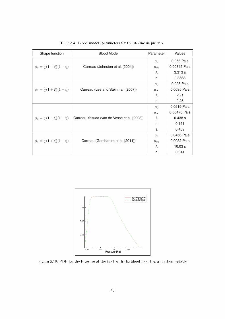
Table 5.4: Blood models parameters for the stochastic process.

Shape function Blood Model Parameter Values

µ0 0.056 Pa·sφ1 = 1

4 (1− ξ)(1− η) Carreau (Johnston et al. [2004]) µ∞ 0.00345 Pa·sλ 3.313 s

n 0.3568

µ0 0.025 Pa·sφ2 = 1

4 (1 + ξ)(1− η) Carreau (Lee and Steinman [2007]) µ∞ 0.0035 Pa·sλ 25 s

n 0.25

µ0 0.0519 Pa·sµ∞ 0.00476 Pa·s

φ3 = 14 (1− ξ)(1 + η) Carreau-Yasuda (van de Vosse et al. [2003]) λ 0.438 s

n 0.191

a 0.409

µ0 0.0456 Pa·sφ4 = 1

4 (1 + ξ)(1 + η) Carreau (Gambaruto et al. [2011]) µ∞ 0.0032 Pa·sλ 10.03 s

n 0.344

Figure 5.16: PDF for the Pressure at the inlet with the blood model as a random variable

46

Figure 5.17: Shear expansion coecients with the blood model as a random variable

Figure 5.18: PDF for the Shear with the blood model as a random variable

47

Table 5.5: Mean and standard deviation values with theblood model as a random variable.



Shear[N] 0.237 ∗ 10−3 0.278 ∗ 10−4





Figure 5.19: Average of the velocity eld with theblood model as a random variable

Figure 5.20: Standard deviation of the velocity eldwith the blood model as a random variable

48

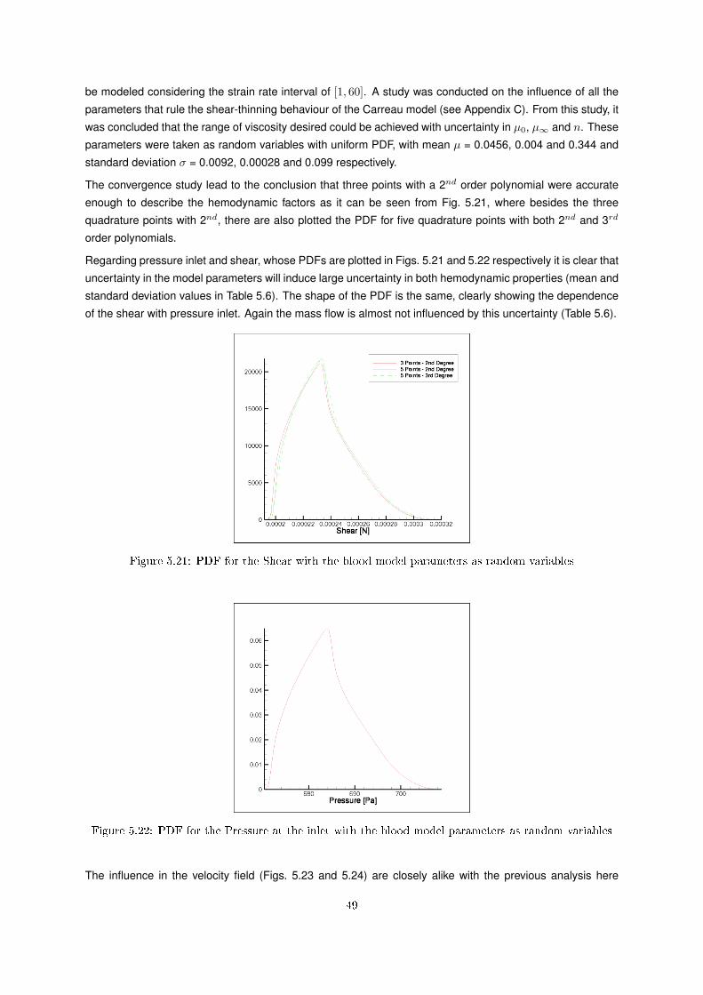
be modeled considering the strain rate interval of [1, 60]. A study was conducted on the influence of all the

parameters that rule the shear-thinning behaviour of the Carreau model (see Appendix C). From this study, it

was concluded that the range of viscosity desired could be achieved with uncertainty in µ0, µ∞ and n. These

parameters were taken as random variables with uniform PDF, with mean µ = 0.0456, 0.004 and 0.344 and

standard deviation σ = 0.0092, 0.00028 and 0.099 respectively.

The convergence study lead to the conclusion that three points with a 2nd order polynomial were accurate

enough to describe the hemodynamic factors as it can be seen from Fig. 5.21, where besides the three

quadrature points with 2nd, there are also plotted the PDF for five quadrature points with both 2nd and 3rd

order polynomials.

Regarding pressure inlet and shear, whose PDFs are plotted in Figs. 5.21 and 5.22 respectively it is clear that

uncertainty in the model parameters will induce large uncertainty in both hemodynamic properties (mean and

standard deviation values in Table 5.6). The shape of the PDF is the same, clearly showing the dependence

of the shear with pressure inlet. Again the mass flow is almost not influenced by this uncertainty (Table 5.6).

Figure 5.21: PDF for the Shear with the blood model parameters as random variables

Figure 5.22: PDF for the Pressure at the inlet with the blood model parameters as random variables

The influence in the velocity field (Figs. 5.23 and 5.24) are closely alike with the previous analysis here

49

Figure 5.23: Average of the velocity eld with theblood model parameters as random variables

Figure 5.24: Standard deviation of the velocity eldwith the blood model parameters as random vari-ables

Table 5.6: Mean and standard deviation values with theblood model parameters as random variables.



Shear[N] 0.234 ∗ 10−3 0.210 ∗ 10−4





50

presented.

5.3.3 Distinctive Models

On another approach to the uncertainty in the blood behaviour, a study was performed to include the blood

model as a stochastic variable. Four different blood models were used (the same models used in sec-

tion 5.3.1). The stochastic variable has an uniform PDF ranging from -1 to 1, with each model having equally

spaced ranges.

As three convergence studies were already presented, in this section no convergence study is shown, how-

ever one was performed and the conclusion was that, for accurate representation of the PDF, ten points with

2nd order polynomials were necessary.

Again big influence in the pressure inlet and shear happens when uncertainty is applied to the blood viscosity

from what can be seen in Figs. 5.25 and 5.26 respectively and almost no influence in mass flow (table 5.7).

The shape of the PDFs is again similar to each other, showing a couple of steps, which are due to the

discontinuities created by the change between one model and the other on the viscosity PDF.

Figure 5.25: PDF for the Shear with the blood model as a random variable

Table 5.7: Mean and standard deviation values with theblood model as a random variable.



Shear[N] 0.237 ∗ 10−3 0.278 ∗ 10−4





The influence in the velocity field (Figs. 5.27 and 5.28) are closely alike with the previous two analysis here

presented.

51

Figure 5.26: PDF for the Pressure at the inlet with the with the blood model as a random variable

Figure 5.27: Average of the velocity eld with theblood model as a random variable

Figure 5.28: Standard deviation of the velocity eldwith the blood model as a random variable

52

5.4 Blood and Geometry Stochastic Inuence

Having studied the influence of the geometry and blood behaviour uncertainty individually, in this section the

combined influence of both uncertainties is studied. This section presents two different subsections. First the

smaller radius is combined with section 5.3.1 and next critical radius is combined with section 5.3.2 in order

to quantify uncertainty of the blood behaviour in both a small and big obtructions.

5.4.1 Smaller Radius and Model Parameters Uncertainty

Having already performed a convergence study for the radius and model parameters individually it assumes

that for the variables combined it is also only necessary three points for each random variable for accurate

results. Moreover, since one of the uncertainties strongly overcomes the other, it is not expected a big

influence from the cross products in the PC expansion.

When comparing the confidence interval of the velocity profile of this analysis (Fig. 5.29) with the one taking

just the radius of the clot as a random variable it is clear that they are very much alike, showing the largest

differences in the recirculation zone (where viscosity plays a more important role).

As for the pressure inlet (Fig. 5.30) it has almost the same PDF behaviour as when considering just the model

parameters.

On the other hand the shear PDF (Fig. 5.31) is more of a combined influence of the thrombosis radius and

the blood model parameters. From Fig. 5.32 is clear that the radius has the most influence in the shear,

however the blood model parameters are also influencing shear as well, leading to the conclusion that the

blood influence is comparable with the geometry uncertainty. This is a large influence as it can be seen from

the standard deviation in table 5.8.

Even with the combination of random variables, the mass flow split becomes almost unchanged (table 5.8).

Table 5.8: Mean and standard deviation values with thethrombosis radius and the blood model parameters as ran-dom variables.



Shear[N] 0.236 ∗ 10−3 0.248 ∗ 10−4





5.4.2 Critical Radius and Model Parameters Uncertainty

It is also important to take a look at the combined effect of the bloo uncertainty with uncertainty in the size of

a large obstruction in order to see if the effect on the hemodynamic factors are also significantly affected by

the blood uncertainty.

53

Figure 5.29: Stochastic parameters of the velocity prole with the thrombosis radius and the blood modelparameters as random variables

Figure 5.30: PDF for the Pressure at the inlet with the thrombosis radius and the blood model parametersas random variables

54

Figure 5.31: PDF for the Shear with the thrombosis radius and the blood model parameters as randomvariables

Figure 5.32: Shear expansion coecients with the radius and the blood model parameters as randomvariables

55

For the velocity profile (Fig. 5.33) the effect of uncertainty is clearly mostly due to the size of the obstruction

as the PDF is closely alike the one when considering just the radius as a random variable (Fig. 5.13).

Taking a look at the PDF of both shear (Fig. 5.34) and pressure inlet (Fig. 5.35) it can be seen the influence of

both the blood and geometry with large standard deviation (Table 5.9). Thus Fig. 5.36 shows the coefficients

of the shear expansion, clearly showing that the radius influence is close to that of one of the blood model

parameters, µinf . No other coefficients are plotted as they had no significance when compared to µinf and

the radius.

Again the mass flow split is affected, still with no great changes as it can be seen in table 5.9 from the

standard deviation.

Figure 5.33: Stochastic parameters of the velocity prole with the thrombosis radius and the blood modelparameters as random variables

Table 5.9: Mean and standard deviation values with thethrombosis radius and the blood model parameters as ran-dom variables.



Shear[N] 0.599 ∗ 10−3 0.140 ∗ 10−3





56

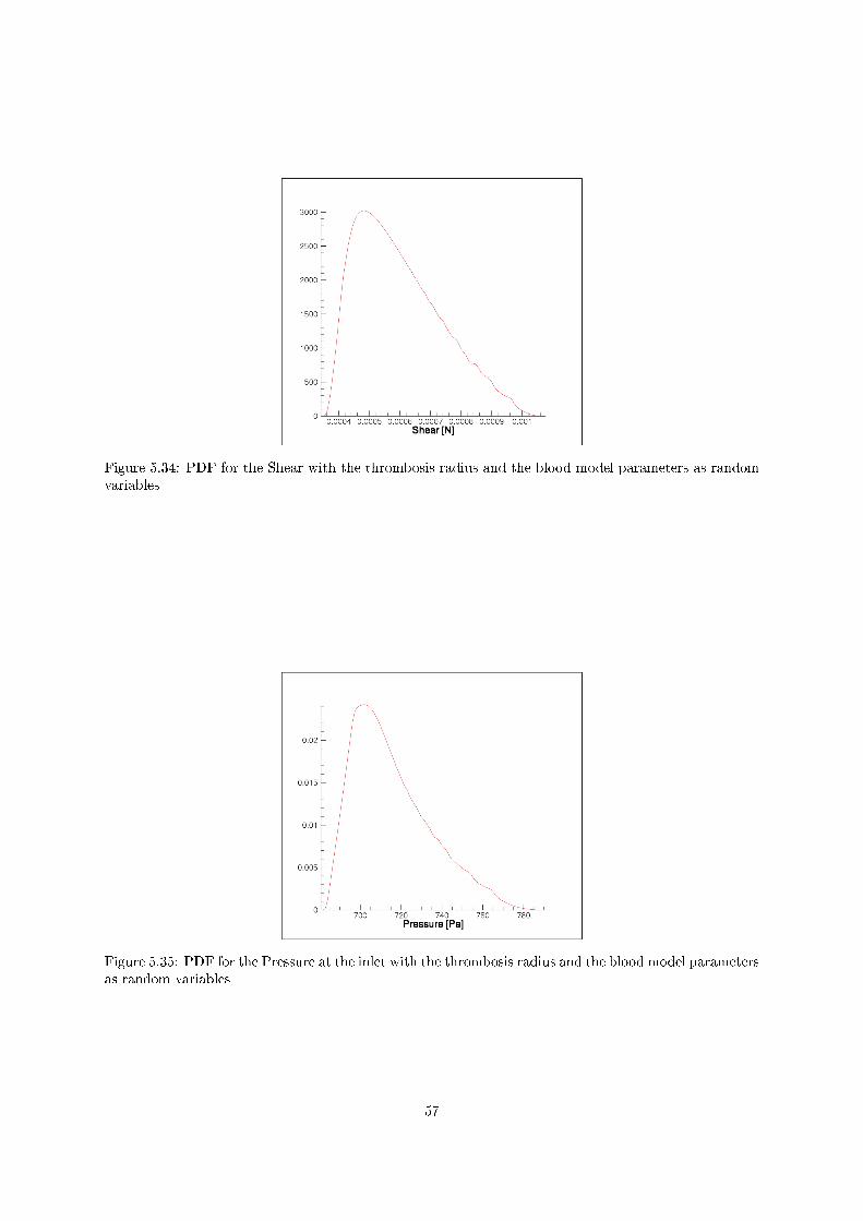
Figure 5.34: PDF for the Shear with the thrombosis radius and the blood model parameters as randomvariables

Figure 5.35: PDF for the Pressure at the inlet with the thrombosis radius and the blood model parametersas random variables

57

Figure 5.36: Shear expansion coecients with the radius and the blood model parameters as randomvariables

58

Chapter 6

Conclusions

As proposed for the objectives of this Thesis, a verification of the numerical code was performed using simple

2D and 3D geometries. Thus the validation of blood flow was made using models and results accepted as

accurate in the scientific community.

The model of the portal vein was studied with a clot in one branch. As the pressure drop in the vein was

modeled taken into account the real pressure drop of the liver, the mass flow split was not affected by the

uncertainties studied in almost all of the analyses. The flow inside the geometry showed predictible behaviour

with a blunter velocity profile than that of a parabolic one due to the shear-thinning behaviour of blood. Around

the clot, a recirculation bubble developed, which with increasing size leads to increasing risk of thrombosis

and an increase in the clot itself. As it was expect the mass flow rate in the branch with the clot was about

double of that in the other branch.

A NISP method was implemented in the geometries examined. For each uncertainty quantification analysis

a convergence study was performed, leading to the conclusion that for the random variables analysed a 2nd

order polynomial with 3 quadrature points gives accurate results. The NISP method allowed for the assembly

of the PDF for each flow factor studied as well as the values for the mean and standard deviation.

A thorough study was developed on the influence of blood viscosity in blood flow. On this note, several blood

viscosity models were studied showing different behaviours for different strain rate ranges. It is possible to

conclude that, for low strain rates there is a great deal of uncertainty associated to the blood behaviour.

Bearing in mind this uncertainty three approaches were investigated for the uncertainty quantification of the

blood viscosity influence in the flow. This investigation tool into account a combination of different blood

models, different blood model parameters and distinctive blood models. The results obtained for the three

analyses showed that even though the range of influence of the three approaches was similar, the shape of

the PDF was very different leading to different uncertainty behaviours. It can be concluded from this study

that the uncertainty in the the blood model can lead to great uncertainty in the shear force in the walls of the

blood vessels, leading to uncertainty regarding the possibility of vein rupture consequent to the appearance

of blood clots.

The uncertainty regarding geometry was also deeply investigated as it was quantified through the several

steps that lead from the real human body to an image of the human body. This lead to a range of values of

59

accuracies from each step that leads to the final image. This uncertainty was quantified with the NISP method

with two different geometries. The first one was a small obstruction, which, having obtained the results from

the uncertainty quantification, was clearly influencing shear and pressure in the vein. The other geometry

studied was a big clot in the artery and the influence of the geometry uncertainty was clearly larger than that

for the small obstruction. Concluding, for critical clots it is even more important to have accurate images of

the geometry, thus uncertainty should be definetely taken into account.

When combining uncertainty from geometry and the blood, the influence of each random variable varies

greatly with the size of the clot. This way with a small clot, the influence of the blood parameters was in the

same order of magnitude as the radius influence. However when it comes to critical geometries, the radius

size has definetely larger influence in the flow development.

This study shows clearly a need for more intense study on the uncertainty regarding blood flow as it is an

area with great potential for diagnosing diseases.

60

References

S. Acharjee and N. Zabarras. A non-intrusive stochastic galerkin approach for modeling uncertainty propa-

gation in deformation processes. Computers and Structures, 85:244–254, 2007.

L. Antiga, B. Ene-Iordache, and A. Remuzzi. Computational geometry for patient-specific reconstruction and

meshing of blood vessels from MR and CT angiography. IEEE Transactions on Medical Imaging, 22(5),

2003.

O. Baskurt, O. Yalcin, and J. Meiselman. Hemorheology and vascular control mechanisms. Clinical Hemorhe-

ology and Microcirculation, 30:169–178, 2004.

A. Bazille, M. Guttman, E. McVeigh, and E. Zerhouni. Impact of semi-automated versus manual image

segmentation errors on myocardial strain calculation by magnetic ressonance tagging. Invest Radiol., 29

(4):427–433, 1994.

C. Bertolotti and V. Deplano. Three-dimensional numerical simulations of flow through a stenosed coronary

bypass. Journal of Biomechanics, 33:1011–1022, 2000.

C. Botar, T. Vasile, S. Sfrangeu, S. Clichici, P. Agachi, and P. Badea. Validation of CFD simulation results in

case of portal vein blood flow. Computer Aided Chemical Engineering, 28:205–210, 2010.

J. Boyd, J. Buick, and S. Green. Analysis of the Casson and Carreau-Yasuda Non-Newtonian blood models

in steady and oscillatory flows using the lattice boltzmann method. Physics of Fluids, 19, 2007.

J. Buchanan, C. Kleinstreuer, G. Truskey, and M. Lei. Relation between non-uniform hemodynamics and sites

of altered permeability and lesion growth at the rabbit aorto-celiac junction. Atherosclerosis, 143:27–40,

1999.

61

J. Chen, X. Lu, and W. Wang. Non-newtonian effects of blood flow on hemodynamics in distal vascular graft

anastomoses. Journal of Biomechanics, 39:1983–1995, 2006.

S. Chien, S. Usami, R. Dellenback, and M. Gregersen. Blood viscosity: Influence of erythrocyte deformation.

Science, 157(3790):827–829, 1967a.

S. Chien, S. Usami, R. Dellenback, and M. Gregersen. Blood viscosity: Influence of erythrocyte aggregation.

Science, 157(3790):829–831, 1967b.

J. A. Esperança Pina. Anatomia Humana dos Órgãos. Lidel, January 2004. ISBN 978-972-757-149-9.

M. Friedman and D. Giddens. Blood flow in major blood vessels - modeling and experiments. Annals of

Biomedical Engineering, 33(12), 2005.

A. Gambaruto, J. Janela, A. Moura, and A. Sequeira. Sensitivity of hemodynamics in a patient specific

cerebral aneurysm to vascular geometry and blood rheology. Mathematical Biosciences and Engineering,

8(2):409–423, 2011.

S. George, D. Martin, and D. Giddens. Portal vein contribution to the right and left lobes of the liver using MRI

and CFD. IFMBE Proceedings, 31:473–476, 2010.

G. Gerig, O. Kubler, R. Kikinis, and F. Jolesz. Nonlinear anisotropic filtering of MRI data. IEEE Transactions

on Medical Imaging, 11(2), 1992.

S. Hammer, A. Jeays, P. Allan, R. Hose, D. Barber, W. Easson, and P. Hoskins. Acquisition of 3-D arterial

geometries and integration with computational fluid dynamics. Ultrasound in Med. & Biol., 35(12):2069–

2083, 2009.

J. Janela, A. Moura, and A. Sequeira. Towards a geometrical multiscale approach to non-newtonian blood

flow simulations. Advances in Mathematical Fluid Mechanics, 2010.

B. Johnston, R. Johnston, S. Corney, and D. Kilpatrick. Non-Newtonian blood flow in human right coronary

arteries: Steady state simulations. Journal of Biomechanics, 37(5), 2004.

M. Kameneva, K. Garrett, M. Watach, and H. Borovetz. Red blood cell aging and risk of cardiovascular

diseases. Clinical Hemorheology and Microcirculation, 18:67–74, 1998.

62

U. Kohler, I. Marshall, M. Robertson, Q. Long, X. Xu, and P. Hoskins. MRI measurement of wall shear

stress vectors in bifurcation models and comparison with CFD predictions. Journal of Magnetic Resonance

Imaging, 14:563–573, 2001.

D. Ku. Blood flow in arteries. Annu Rev Fluid Mech, 29:399–434, 1997.

D. Ku, D. Giddens, C. Zarins, and S. Glagov. Pulsatile flow and atherosclerosis in the human carotid bi-

furcation. Positive correlation between plaque location and low oscillating shear stress. Arteriosclerosis,

Thrombosis, and Vascular Biology, 5:293–302, 1985.

S. Lee and D. Steinman. On the relative importance of rheology for image-based CFD models of the carotid

bifurcation. J. Biomech. Eng., 129(2):273–279, 2007.

A. Marossy, P. Svorc, I. Kron, and S. Gresová. Hemorheology and circulation. Clinical Hemorheology and

Microcirculation, 42:253–258, 2009.

M. Mendes. Modeling and Simulation of Hydrocarbon Oxidation Processes within Porous Inert Media. PhD

thesis, Instituto Superior Técnico - Universidade Técnica de Lisboa, July 2010.

C. Millet-Bex. O Corpo Humano - Parte 2. Grande Biblioteca Médica. Granroma Editores, 2005.

J. Milner, J. Moore, B. Rutt, and D. Steinman. Hemodynamics of human carotid artery bifurcations: Compu-

tational studies with models reconstructed from magnetic resonance imaging of normal subjects. Journal

of Vascular Surgery, 28(1):143–156, 1998.

A. Miranda, P. Oliveira, and Pinho F. Steady and unsteady laminar flows of Newtonian and generalized

Newtonian fluids in a planar T-junction. International Journal for Numerical Mehtods in Fluids, 57:295–328,

2008.

K. Moyle, L. Antiga, and D. Steinman. Inlet conditions for image-based CFD models of the carotid bifurcation:

Is it reasonable to assume fully developed flow? Journal of Biomechanical Engineering, 128, 2006.

R. Nowak. Wavelet-based rician noise removal for magnetic resonance imaging. IEEE Transactions on Image

Processing, 8, 1999.

63

W. Oberkampf and T. Trucano. Verification and validation in computational fluid dynamics. Progress in

Aerospace Sciences, 38:209–272, 2002.

E. Ofili, J. Kern, J. St. Vrain, T. Donohue, R. Bach, B. Al-Joundi, F. Aguirre, R. Castello, and A. Labovitz. Differ-

ential characterization of blood flow, velocity and vascular resistance between proximal and distal normal

epicardial human coronary arteries: Analysis by intracoronary doppler spectral flow velocity. American

Heart Journal, 130(1):37–46, 1995.

S. Patankar and D. Spalding. A calculation procedure for hear, mass and momentum transfer in three-

dimensional parabolic flows. International Journal of heat and Mass Transfer, 15(10):1787–1806, 1972.

K. Perktold and G. Rappitsch. Computer simulation of local blood and vessel mechanics in a compliant

carotid artery bifurcation model. Journal of Biomechanics, 28(7):845–856, 1955.

K. Perktold, M. Hofer, G. Rappitsch, M. Loew, B. Kuban, and M. Friedman. Validated computation of physio-

logic flow in a realistic coronary artery branch. Journal of Biomechanics, 31:217–228, 1998.

S. Petkova. Investigation of portal vein blood flow in cirrhotic portal hypertension using computer-based and

physical modelling methods. PhD thesis, Swinburne University of Technology, 2008.

S. Petkova, A. Hossain, J. Naser, and E. Palombo. CFD modelling of blood flow in portal vein hyperten-

sion with and without thrombosis. Third International Conference on CFD in the minerals and Process

Industries, pages 527–530, 2003.

A. Popel and P. Johnson. Microcirculation and hemorheology. Annu Rev Fluid Mech, 37:43–69, 2005.

M. Reagan, H. Najm, G. Ghanem, and O. Knio. Uncertainty quantification in reacting-flow simulations through

non-intrusive spectral projection. Combustion and Flame, 132:545–555, 2003.

A. Robertson, A. Sequeira, and M. Kameneva. Hemodynamical Flows. Modeling, Analysis and Simulation,

volume 37. Oberwolfach Seminars, 2008.

R. Rosenson, S. Shott, and C. Tangney. Hypertriglyceridemia is associated with an elevated blood viscosity

Rosenson: triglycerides and blood viscosity. Atherosclerosis, 161:433–439, 2002.

64

S. Sankaran and A. Marsden. A stochastic collocation method for uncertainty quantification and propagation

in cardiovascular simulations. Journal of Biomechanical Engineering, 133, 2011.

A. Sequeira and J. Janela. An overview of some mathematical models of blood rheology. A Portrait of

State-of-the-Art Research at the Technical University of Lisbon, pages 65–87, 2007.

E. Shaik, K. Hoffmann, and J. Dietiker. Numerical simulations of pulsatile Non-Newtonian flow in an end-to-

side anastomosis model. Simulation Modelling Practice and Theory, 16:1123–1135, 2008.

S. Shibeshi and W. Collins. The rheology of blood flow in a branched arterial system. Applied Rheology, 15

(6):398–405, 2005.

M. Siouffi, V. Deplano, and R. Pélissier. Experimental analysis of unsteady flows through a stenosis. Journal

of Biomechanics, 31:11–19, 1998.

P. Stein and H. Sabbah. Turbulent blood flow in the ascending aorta of human with normal and diseased

aortic valves. Circulation Research, 39:58–65, 1976.

C. Tu and M. Deville. Pulsatile flow of Non-Newtonian fluids through arterial stenoses. Journal of Biomechan-

ics, 29(7):899–908, 1996.

F. van de Vosse, J. Hart, C. Oijen, D. Bessems, T. Gunther, A. Segal, B. Wolters, J. Stijnen, and F. Baai-

jens. Finite-element-based computational methods for cardiovascular fluid-structure interaction. Journal of

Engineering Mathematics, 47:335–368, 2003.

J. Vimmr and A. Jonásová. Non-Newtonian effects of blood flow in complete coronary and femoral bypasses.

Mathematics and Computers in Simulation, 80:1324–1336, 2010.

D. Wang and J. Bernsdorf. Lattice Boltzmann simulation of steady Non-Newtonian blood flow in a 3D generic

stenosis case. Computers and Mathematics with Applications, 58:1030–1034, 2009.

D. Xiu and G. Karniadakis. The Wiener-Askey polynomial chaos for stochastic differential equations. SIAM

J. SCI. COMPUT., 24(2):619–644, 2002a.

D. Xiu and G. Karniadakis. Modeling uncertainty in steady state diffusion problems via generalized polynomial

chaos. Computer Methods in Applied Mechanics and Engineering, 191(43):4927–4948, 2002b.

65

D. Xiu, D. Lucor, C. Su, and G. Karniadakis. Stochastic modeling of flow-structure interactions using gener-

alized polynomial chaos. Journal of Fluids Engineering, 124(1):51–59, 2002.

Y. Yang, S. George, D. Martin, A. Tannenbaum, and D. Giddens. 3D modeling of patient-specific geometries

of portal veins using MR images. Engineering in Medicine and Biology Society, 28th Annual International

Conference of the IEEE, 2006.

F. Yilmaz and M. Gundogdu. A critical review on blood flow in large arteries; relevance to blood rheology,

viscosity models, and physiologic conditions. Korea-Australia Rheology Journal, 20(4):197–211, 2008.

66

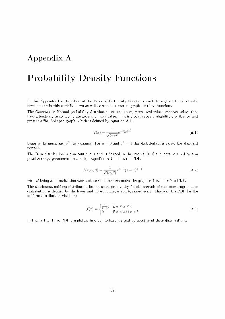
Appendix A

Probability Density Functions

In this Appendix the denition of the Probability Density Functions used throughout the stochasticdevelopment in this work is shown as well as some illustrative graphs of these functions.

The Gaussian or Normal probability distribution is used to represent real-valued random values thathave a tendency to conglomerate around a mean value. This is a continuous probability distribution andpresent a bell-shaped graph, which is dened by equation A.1.

f(x) =1√

2πσ2e

−(x−µ)2

2σ2 (A.1)

being µ the mean and σ2 the variance. For µ = 0 and σ2 = 1 this distribution is called the standardnormal.

The Beta distribution is also continuous and is dened in the interval [0,1] and parametrized by twopositive shape parameters (α and β). Equation A.2 denes the PDF.

f(x, α, β) =1

B(α, β)xα−1(1− x)β−1 (A.2)

with B being a normalization constant, so that the area under the graph is 1 to make it a PDF.

The continuous uniform distribution has an equal probability for all intervals of the same length. Thisdistribution is dened by the lower and upper limits, a and b, respectively. This way the PDF for theuniform distribution yields in:

f(x) =

1b−a , if a ≤ x ≤ b0 if x < a ∪ x > b

(A.3)

In Fig. A.1 all three PDF are plotted in order to have a visual perspective of these distributions.

67

Figure A.1: Probability density functions

68

Appendix B

Numerical Methods

As stated in Chapter 3, in order to solve the coecients' integrals, a numerical method is used. When theinput variable has a Gaussian PDF, and therefore is discretized with Hermite polynomials, the numericalmethod used is the Gauss-Hermite quadrature. On the other hand, for a Beta distribution, with Jacobipolynomials, the method is a Gauss-Jacobi quadrature, while for an uniform distribution the quadratureused is Gauss-Legendre with Legendre orthogonal polynomials.

A quadrature rule is an approximation of the denite integral of a function, usually stated as a weightedsum of function values at specied points within the domain of integration. This method providesaccurate results for polynomials of degree 2n− 1, being n the number of points used in the quadrature.Even though the domain of integration is restricted to [−1, 1], which equation for the quadrature yieldsin equation B.1, the interval can be changed to [a, b] by applying equation B.2.

B.1 Gauss-Legendre Quadrature

For the Gauss-Legendre quadrature wi is given by equation B.3.

∫ 1

−1

f(x)dx =

∫ 1

−1

W (x)g(x) ≈n∑i=1

wif(xi) (B.1)

∫ b

a

f(x)dx ≈ b− a2

n∑i=1

wif

(b− a

2xi +

b+ a

2

)(B.2)

wi =2

(1− x2i ) [P ′n(xi)]

2 , where Pn(x) is the nth Legendre polynomial (B.3)

B.2 Gauss-Hermite Quadrature

This method is used for integrals in the form of

∫ ∞−∞

e−x2

f(x)dx ≈n∑i=1

wif(xi) (B.4)

with

wi =2n−1n!

√π

n2 [Hen−1(xi)]2 (B.5)

69

B.3 Gauss-Jacobi Quadrature

This method is used for integrals in the form of

∫ 1

−1

f(x)(1− x)α(1 + x)βdx =

∫ 1

−1

W (x)g(x) ≈n∑i=1

λif(xi) (B.6)

with

λi = −2n+ α+ β + 2

n+ α+ β + 1

Γ(n+ α+ 1)Γ(n+ β + 1)

Γ(n+ α+ β + 1)(n+ 1)!

2α+β

P ′n(xi)Pn+1(xi)(B.7)

70

Appendix C

Parameter Inuence in the Blood

Carreau Model

In this Appendix is presented the study performed on the inuence of the Carreau model parameters (µ0,µ∞, n and λ). Taking in consideration a Carreau model with mean values for its parameters (µ0 = 0.0456Pa.s, µ∞ = 0.004 Pa.s, n = 0.344 and λ = 10.03 s), each parameter was taken as a variable with a certainstandard deviation and studied individually and colectively. For comparison purposes, the four bloodviscosity models used in section 5.3 were plotted in black in all of the gures in this Appendix, in orderto help evaluate the correct range of blood viscosity within the strain rate range considered.

In Figs. C.1-C.4 µ0, µ∞, n and λ, are studied individually, respectively, with its mean value and avariation of 30% of that value. It can be seen that λ is the least inuenciable parameter on the bloodviscosity and therefore were disregarded as a random variable. µ0, µ∞ and n show big inuence in theblood viscosity, however n shows inuence evenly throughout the range, whereas µ0 and µ∞ show greaterinuence in the beginning and in the end of the range respectively.

The best t to the four models in black is obtained by combining three parameters (µ0, µ∞ and n) withstandard deviations of 0.00923, 0.00027 and 0.099 for µ0 and µ∞ and n, respectively (Fig. C.5).

Figure C.1: Study on the inuence of µ0

71

Figure C.2: Study on the inuence of µ∞

Figure C.3: Study on the inuence of λ

Figure C.4: Study on the inuence of n

72

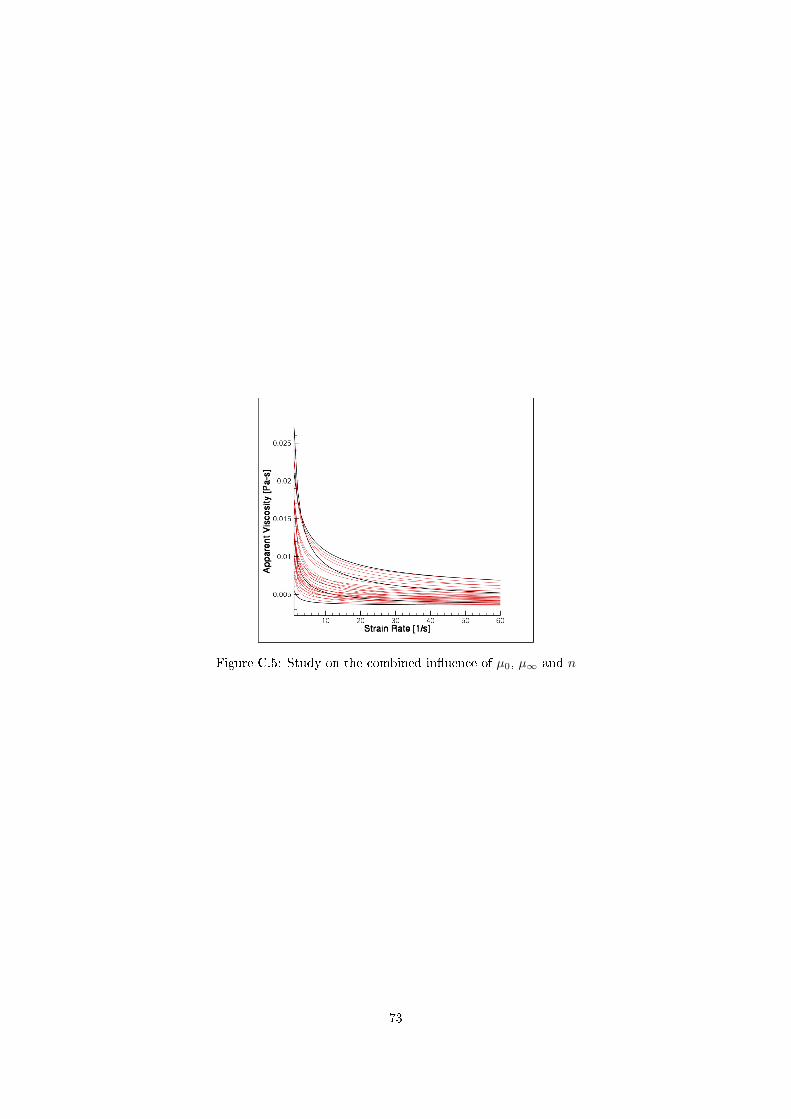
Figure C.5: Study on the combined inuence of µ0, µ∞ and n

73

Analysis and Simulation of Blood Flow in the Portal Vein ... · Analysis and Simulation of Blood...

Documents

Transcript of Analysis and Simulation of Blood Flow in the Portal Vein ... · Analysis and Simulation of Blood...