SPTECHCON - Rev Your Engines - SharePoint 2013 Performance Enhancements

1
ANALYSIS AND PERFORMANCE ENHANCEMENTS IN POWER LINE, WIRELESS AND MOBILE NETWORKS
By
SUNGUK LEE
A DISSERTATION PRESENTED TO THE GRADUATE SCHOOL OF THE UNIVERSITY OF FLORIDA IN PARTIAL FULFILLMENT
OF THE REQUIREMENTS FOR THE DEGREE OF DOCTOR OF PHILOSOPHY
UNIVERSITY OF FLORIDA
2010

2
© 2010 Sunguk Lee

3
To my parents and my wife Hyuna Kim

4
ACKNOWLEDGMENTS
First of all, I would like to express my deep appreciation for my academic advisor,
Dr. Haniph A. Latchman for his patient guidance, encouragement and plentiful advice
until I can successfully finish my Doctoral research. I would also like to thank the
members of my PhD. committee, Dr. Arroyo, Dr. Janise McNair, and Dr. Fitz-Coy. I am
grateful for their willingness to serve on my committee and their helpful advice.
I thank my parents who have kept encouraging and inspiring me to pursue my
dream in many ways with unconditional love. I have to thank my lovely wife, Hyuna Kim.
She has patiently and enthusiastically supported my study.
I also thank my colleagues at Laboratory for Information Systems and Tele-
communications (LIST) in ECE department for their many helpful and friendly
discussions that always gave me a new realization.

5
TABLE OF CONTENTS page
ACKNOWLEDGMENTS ...................................................................................................... 4
LIST OF TABLES ................................................................................................................ 7
LIST OF FIGURES .............................................................................................................. 8
ABSTRACT........................................................................................................................ 10
CHAPTER
1 INTRODUCTION ........................................................................................................ 12
Home Network ............................................................................................................ 12 Mobility Management Protocol ................................................................................... 14
2 COMPARATIVE PERFORMANCE ANALYSIS OF LOCAL AREA NETWORK TECHNOLOGIES FOR MULTIMEDIA STREAMING IN HOME ............................... 16
Introduction ................................................................................................................. 16 Overview of Wireless LAN and Powerline communication ....................................... 16
IEEE 802.11x Wireless LAN ................................................................................ 17 Power Line Communication ................................................................................. 18
Experiment Setup ....................................................................................................... 22 Test of UDP and TCP Protocol .................................................................................. 25
3 A VISUALIZATION TOOL FOR NETWORKING PROTOCOL ANALYSIS .............. 32
Introduction ................................................................................................................. 32 Requirements .............................................................................................................. 34 Design and Implementation........................................................................................ 35
Design of the EVGator User Interface ................................................................. 36 Configuring the EVGATOR .................................................................................. 40 Trace File Format ................................................................................................. 40 Zoom – In/Out ...................................................................................................... 42
Experience .................................................................................................................. 43 Conclusion .................................................................................................................. 44
4 ENHANCED LIMITED ROUND ROBIN MECHANISM USING PRIORITY POLICY OVER BLUETOOTH NETWORK ................................................................ 45
Introduction ................................................................................................................. 45 MAC scheduling scheme of Bluetooth ....................................................................... 46 ELRR-PP Algorithm .................................................................................................... 49

6
Performance Evaluation ............................................................................................. 51 Conclusion .................................................................................................................. 54
5 EFFICIENT MOBILITY MANAGEMENT SCHEME OVER WIRELESS LOCAL AREA NETWORK ....................................................................................................... 56
Introduction ................................................................................................................. 56 Enhanced Handover Scheme of MIPv6 with Fast Movement Detection & DAD ..... 57
Overview of MobileIPv6 (MIPv6) ......................................................................... 57 Proposed MIPv6 Handover Scheme with FMDD................................................ 60
Movement Detection using Stored RA message ......................................... 61 DAD configuration and Lookup Algorithm .................................................... 62
Efficient PMIPv6 Handover Scheme over Wireless Local Area Network ................. 64 Overview of Proxy Mobile IPv6 (PMIPv6) ........................................................... 64 Proposed PMIPv6 protocol 1 ............................................................................... 66
L2 Handover Procedure ................................................................................ 66 L3 Handover Procedure ................................................................................ 67
Proposed PMIPv6 Protocol 2 .............................................................................. 71 Analytical model .......................................................................................................... 73 Performance Analysis ................................................................................................. 77
Analysis of Handover Latency and Packet Loss................................................. 78 Mobile IPv6. ................................................................................................... 79 Proxy Mobile IPv6 ......................................................................................... 81 Proposed PMIPv6 Protocol 1 ........................................................................ 82
Analysis of Signaling Cost ................................................................................... 83 Mobile IPv6 Protocol ..................................................................................... 85 Proxy Mobile IPv6 protocol ........................................................................... 86 Proposed PMIPv6 Protocol 2 ........................................................................ 87
Numerical Result and Comparison ............................................................................ 88 Numerical Result of MIPv6 with FMDD ........................................................ 89 Numerical Result of Proposed PMIPv6 Scheme 1 ...................................... 92 Numerical Result of Proposed PMIPv6 scheme 2 ....................................... 97
Conclusion .................................................................................................................. 99
6 CONCLUSIONS........................................................................................................ 100
LIST OF REFERENCES ................................................................................................. 102
BIOGRAPHICAL SKETCH.............................................................................................. 106

7
LIST OF TABLES
Table page 2-1 PLC Adaptors ......................................................................................................... 24
2-2 Classification of video streaming ........................................................................... 30
2-3 Quality of 25Mbps, HD video streaming ................................................................ 30
4-1 Priority Scheme ...................................................................................................... 50
4-2 Traffic Generation Parameter ................................................................................ 53
5-1 D flag in NRA message .......................................................................................... 63
5-2 H flag of ENS message .......................................................................................... 69
5-3 A flag of END message .......................................................................................... 70
5-4 Parameters ............................................................................................................. 78
5-4 Parameters for analysis ......................................................................................... 89

8
LIST OF FIGURES
Figure page 2-1 DCF access scheme .............................................................................................. 17
2-2 Beacon period structure of Home Plug AV ........................................................... 19
2-3 TDMA allocation Of Home Plug AV. ...................................................................... 19
2-4 CSMA scheme in HomePlug AV ........................................................................... 20
2-5 Transmission sequence of UPA/DHS.................................................................... 21
2-6 Hybrid Medium Access Protocol ............................................................................ 22
2-7 Test floor plan ......................................................................................................... 23
2-8 Snapshot of Gatorbytes ......................................................................................... 24
2-9 PLC test configuration ............................................................................................ 25
2-10 IEEE 802.11g/n test configuration ......................................................................... 25
2-11 Link coverage versus TCP throughput .................................................................. 26
2-12 Link coverage versus UDP throughput .................................................................. 27
2-13 TCP throughput versus distance of direct path ..................................................... 28
2-14 UDP throughput versus distance of direct path .................................................... 29
3-1 Text versus graphical event analyzer .................................................................... 37
3-2 Example of selecting desired events. .................................................................... 40
3-3 EVGATOR configuration format ............................................................................ 41
3-4 Generated trace log file format .............................................................................. 41
3-5 Example of actual display window ......................................................................... 42
4-1 MAC Scheduling scheme of Bluetooth .................................................................. 47
4-2 Flow chart of ELRR-PP .......................................................................................... 51
4-3 Average delay with same arrival rate .................................................................... 52
4-4 Throughput with variant traffic load ....................................................................... 53

9
4-5 Average delay with variant traffic .......................................................................... 54
5-1 Mobile IPv6 handover procedure ........................................................................... 58
5-2 Mobile IPv6 handover procedure with FMDD Scheme ......................................... 60
5-3 PMIPv6 handover procedure ................................................................................. 65
5-4 Proposed PMIPv6 handover procedure ................................................................ 68
5-5 IAPP MOVE notify packet format........................................................................... 72
5-6 The proposed PMIPv6 scheme in IEEE 802.11 network. ..................................... 73
5-7 Network Configuration............................................................................................ 74
5-8 timing diagram of MIPv6 ........................................................................................ 80
5-9 Timing diagram of PMIPv6..................................................................................... 81
5-10 Timing diagram of proposed scheme1 .................................................................. 83
5-11 Network topology................................................................................................... 88
5-12 Mobile IPv6 handover latency comparison 1 ........................................................ 90
5-13 Mobile IPv6 handover latency comparison 2 ........................................................ 91
5-14 Mobile IPv6 handover latency comparison 3 ........................................................ 91
5-15 PMIPv6 handover latency comparison 1 ............................................................... 92
5-16 PMIPv6 handover latency comparison 2 ............................................................... 93
5-17 PMIPv6 handover latency comparison 3 ............................................................... 94
5-18 PMIPv6 packet loss comparison 1 ........................................................................ 95
5-19 PMIPv6 packet loss comparison 2 ........................................................................ 95
5-20 PMIPv6 packet loss comparison 3 ........................................................................ 96
5-21 Packet delay in session time ................................................................................. 96
5-22 PMIPv6 cost comparison 1 .................................................................................... 97
5-23 PMIPv6 cost comparison 2 .................................................................................... 98
5-24 PMIPv6 cost comparison 3 .................................................................................... 98
10
Abstract of Dissertation Presented to the Graduate School of the University of Florida in Partial Fulfillment of the Requirements for the Degree of Doctor of Philosophy
ANALYSIS AND PERFORMANCE ENHANCEMENTS IN POWER LINE, WIRELESS
AND MOBILE NETWORKS By
Sunguk Lee
May 2010
Chair: Haniph A. Latchman Major: Electrical and Computer Engineering
This dissertation focuses on the study of the performance of Powerline
Communication (PLC), wireless and mobile networks in conveying multimedia traffic
such as Internet Protocol Television (IPTV).
We provide a comprehensive protocol performance comparison for wireless and
PLC in-home networks. Our result shows that the throughput of Homeplug AV is at least
18Mbps higher than that of IEEE 802.11 (g and n) because of improved design and the
quasi-stationary channel characteristics of PLC. We also show that Homeplug AV
outperforms other competing PLC technologies by as much as 17.5% for TCP and 77.7%
for UDP at 77% of connections and in addition achieves 100% full home coverage in
our performance evaluation.
We also developed and used in this work a network protocol visualization tool,
“Visugator” for performance evaluation of network protocols. This tool has been made
freely available for public use.
For distributing multimedia traffic in mobile networks a mobility management
protocol is an essential element of mobile computing including mobile IPTV. We
developed a Fast Movement Detection and DAD (Duplicate Address Detection) (FMDD)

11
scheme for Mobile IPv6 protocol, as well as two improved network-based Proxy Mobile
IPv6 protocols over wireless local area network that reduce handover latency and
signaling overhead. In the Mobile IPv6 with FMDD scheme, the neighbor cache is used
for DAD to reduce the handover latency. To reduce the handover latency and packet
loss of Proxy Mobile IPv6, simultaneous L2 & L3 handover procedures and a tunnelling
scheme are used. With the help of an Inter Access Point Protocol (IAPP) we decrease
the signaling overhead of Proxy Mobile IPv6 significantly. A mathematical analysis is
provided to show the benefits of our proposed schemes. Based on our analytical results,
the FMDD scheme with Mobile IPv6 can reduce the DAD latency by lookup delay in
RAM from the 1 second to just several microseconds. Our proposed Proxy mobile IPv6
protocols also can reduce up to 12.7% of the handover latency, 29.56% of packet loss
and 31.6% of signaling overhead compared with the conventional Proxy Mobile IPv6.
The dissertation also presents a MAC scheduling scheme of Bluetooth to improve
MAC efficiency.

12
CHAPTER 1 INTRODUCTION
Until now several technologies for Local Area Network (LAN) have been
developed and utilized for many applications. Recently the demand for high speed LAN
technologies has increased greatly to support the deployment of high definition video
streaming as HDTV has become more wide spread. Wireless LAN technology is
gaining attention to provide high speed service at hotspots in public areas like an airport
and train station as a part of mobile cellular networks or independent systems using
LAN technologies designed for indoor applications.
Home Network
Many LAN technologies have been competing for preeminence as the multimedia
home networking technology of choice. HDTV is usually encoded in about 25Mbps, and
so to stream one or more HDTV signal requires networks with sustained data rates of
more than 30Mbps at the application layer.
While traditional Ethernet networks with appropriate QoS enabled switches may
be one desirable choice for this purpose as it is a mature technology that supports very
high bit rates, this may not be viable solution for deployment in existing buildings due to
the inconvenience in laying the Ethernet cables around the house with the associated
drilling through dry walls or even concrete walls. Thus wireless and the so-called ‘no
new wires’ solutions become the top contenders for retrofitting a home network in
existing buildings
For some time there has been strong interest in the 802.11x wireless LAN
technologies as key candidates for home networking as these wireless technologies
provide the ultimate convenience and mobility to users. The widely used 802.11b [1] is
13
now considered to be less desirable for streaming HDTV because of its low data rate.
However, the IEEE 802.11g [2] provides raw data rates up to 54Mbps which may
provide enough application level bandwidth to support streaming HDTV. The IEEE
Draft 802.11n standard [3] has also been proposed for higher throughput and QoS
enhancements. It is expected to provide raw data rates up to 600Mbps and
interoperability with IEEE 802.11a/b/g.
Bluetooth [4] is a wireless technology that allows communication devices and
accessories to interconnect using a short-range, low-power, inexpensive radio. While
initially developed to eliminate the numerous short-range cables involved in
interconnecting mobile devices (laptops, mobile phones, headsets, PDAs, etc) in small
networks, usually referred to as PANs (Personal Area Networks), Bluetooth has
expanded in scope to encroach on wireless LANs.
In the class of ‘no new wires’ networks, Power Line Communication (PLC), MoCA
[5] and HomePNA [6] re-use existing wires for communication and claim multimedia in
home streaming capabilities for one or more channels of HDTV. MoCA uses coaxial TV
cable for communication and provides raw data rate as high as 270Mbps, however the
lack of available access points limits its applications. The HomePNA has similar
drawback as the number of telephone jacks in a home are limited and are usually in a
very inconvenient locations for installing HDTV players or recorders or the similar
devices.
Power Line Communication (PLC) uses the existing in home power circuit to
deliver digital data and is considered to be a potentially desirable candidate for home
networks as there are plenty of outlets in a home and they are in convenient locations.

14
In PLC, there are several competing groups – The Home Plug Power Line Alliance and
The Universal Power line Association (UPA) as well as Consumer Electronics Power
line Communication Alliance (CEPCA).
The Home plug AV [7] standard is the most recent enhancement of the 14 Mbps
HomePlug 1.0 standard released by the Home Plug Power line alliance and it provides
200Mbps raw data rate explicitly targeted to support distributing data and high quality,
multistream videos like HDTV and SDTV. UPA [8] proposed the Digital Home
Specification (DHS) with the chip-sets designed by DS2, Spain. It provides 200 Mbps
data rate for AV streaming while the HD-PLC (High Definition power line communication)
[9] by Panasonic, is able to support raw data rate up to 190 Mbps.
Mobility Management Protocol
Currently wireless local area network (WLAN) is widely spread as infrastructures
for high speed wireless service not only in small indoor area but also in hot spots of
public area.
The series of IEEE 802.11 standard are most widely deployed WLAN technology
now days. The popularity of WLAN lies on its low cost and high data rate. The IEEE
802.11 b/g [1,2] uses license-free 2.4 GHz Industrial Scientific and Medical (ISM) ratio
band. The IEEE 802.11g/a [2, 10] can support data rate up to 54Mbps. Since the IEEE
802.11 standard provides link layer roaming a mobile user (MN) can move to another
AP without disruption of current connection within the same network. However WLAN
technology cannot support seamless communication when a mobile user moves to
another network which has a unique network address.
To provide IP level mobility the Mobile Internet Protocol [11] called MIPv4/v6 was
proposed by the Mobile IP working group in the Internet Engineering Task Force (IETF).

15
Though MIPv6 has been developed it cannot fulfill the QoS requirement of real-time
application because of handover latency. In order to reduce the handover latency Fast
handover for Mobile IPv6 (FMIPv6) [12] has been also proposed by IEFT. In FMIPv6 a
mobile user obtains the new CoA before actual handover. This scheme can reduce
delay of Duplicate Address Detection (DAD) which consumes almost handover latency
in the MIPv6. Also Hierarchical Mobile IPv6 (HMIPv6) [13] has been proposed to
improve performance of MIPv6. This protocol minimizes the signaling cost and latency
of location update of MN by adopting a local anchor point called Mobility Anchor Point
(MAP). HMIPv6 is more efficient when MNs are frequently changes their point of
attachment to the network. While several improved MIP schemes have been proposed
until now MIP v6 has not spread widely in practice. MIPv6 and its enhanced schemes
called host based mobility management protocol require to modify protocol stack of MN
for supporting them. This modification causes incensement of complexity and power
consumption of MN.
Recently a network based mobility management protocol named Proxy Mobile
IPv6 (PMIPv6) [14] has been proposed by IETF NetLMM (Network-based Localized
Mobility Management) working group. In PMIPv6 the serving network performs signaling
of IP mobility management on behalf of MN. Therefore no modification of protocol stack
in MN is necessary. In the PMIPv6 domain MN recognizes that it is always in home
network. Though PMIPv6 is superior it also suffers from packet loss and handover
latency.

16
CHAPTER 2 COMPARATIVE PERFORMANCE ANALYSIS OF LOCAL AREA NETWORK
TECHNOLOGIES FOR MULTIMEDIA STREAMING IN HOME
Introduction
A major driving force for the development of advanced high speed in local area
networks especially for home is the need to support the ongoing deployment of high
definition digital television at rates of about 25 Mbps. HDTV signals may originate at one
point in the home from a media center player or via satellite or cable TV. It will then be
the necessary to transport the HDTV signal throughout the home for playing the video
and audio at multiple locations or for remote recording. Streaming HDTV places very
stringent Quality of Service (QoS) requirements on the underlying home networking
technology in terms of delays, jitter and packet loss probabilities.
This chapter presents a study of effective technologies for high speed LAN and
high definition (HD) video streaming applications in a home or small office environment,
without the need for installing new wires. HD videos usually are encoded at a data rate
of about 25Mbps and modern LANs offer throughput of 10 – 100Mbps. Thus a practical
home networking infrastructure should provide 30Mbps or more at the application layer.
Powerline communication (PLC) and wireless networking are among the most desirable
choices of building a home network because of easy installation, with no new wires
needed.
The main contribution of this chapter is to analyse and conduct a real world
performance assessment of the above recent wireless and PLC network technology for
home and small office environments.
Overview of Wireless LAN and Powerline communication
This section gives a brief overview of wireless and power line communication

17
technologies considered in the rest of the paper.
IEEE 802.11x Wireless LAN
There are two accessing methods in IEEE 802.11x technology [1,2], one is DCF
(Distributed Coordination Function) and the other is PCF (Point Coordination Function).
The infrastructure network works with DCF and PCF while ad hoc network uses DCF.
The principal approach of DCF is Carrier Sense Multiple Access with Collision
Avoidance (CSMA/CA). The basic DCF Access scheme is shown in Figure 2-1.
Figure 2-1. DCF access scheme
To avoid collision, physical carrier sense and virtual carrier sense are used and
the physical layer uses these techniques to sense whether the medium is busy or idle.
Whenever a machine decides to send a frame, a duration is specified in the duration
field of the frame to indicate the ending time of the transmission. Other machines that
receive the message update their local NAV (Network Allocation Vector) thus avoiding
the possible collision resulting from more than one node sending frames at the same
time.
The IEEE 802.11g [2] is operated at 2.4GHz band using Orthogonal Frequency
Division Multiplexing (OFDM). The use of the same frequency band makes 802.11g

18
interoperability with IEEE 802.11b while providing a compatible data rate with IEEE
802.11a which uses 5 GHz band. The default minimum contention window size in IEEE
802.11b[ 1] is 31 slots and the slot time is 20µs. IEEE802.11g for compatibility, uses the
same parameters. However, when no IEEE 802.11b stations are present in the network,
IEEE 802.11g will use 15 slots as the minimum window size and 9 µs for slot time to
provide lower protocol overhead and higher throughput.
The IEEE802.11n [3] uses OFDM-MIMO (Multi Input Multi Output) technology and
supports not only 20 MHz channel like IEEE 802.11a/b/g standards but also 40 MHz
channels in physical layer. The performance at MAC layer of IEEE 802.11n is enhanced
by aggregating several frames into one transmission frame. The frame aggregation can
decrease the transmission time of preamble and frame header under ideal channel
conditions. However, the corruption of aggregation frame will reduce the MAC efficiency
as the long channel time is wasted.
Power Line Communication
The Home plug AV [7] operates in the 2-28MHz band and it uses windowed
OFDM and Turbo Convolution Code (TCC) in the physical layer. The MAC layer uses a
mix of TDMA and CSMA and supports QoS (Quality of Service). There is a Central
Coordinator (CCo) in each of the PLC networks. The CCo broadcasts a periodical
beacon frame with information of TDMA and CSMA allocations at the beginning of each
beacon period. This beacon period is synchronized with the AC line cycle. Figure 2-2
shows the Home Plug AV’s beacon period structure.
The TDMA allocation is for applications that demand QoS while the CSMA
allocation is used by applications that do not have strict QoS requirements. The

19
allocations of TDMA slots in Home Plug AV is dynamic. Figure 2-3 shows TDMA
allocation of Home Plug AV.
Beacon Region TDMA Allocation CSMA Allocation
Dyanmic TDMA Alloc. Session # 1
Dyanmic TDMA Alloc. Session # 2
Beacon Period
Figure 2-2. Beacon period structure of Home Plug AV
TDMA Session # 1 CSMA
Beacon
Payload SACKRTS CTS SOF
RTS- CTS Gap (100us)
CTS- SOF Gap (100us)
Response Gap (100us)
Only used under hidden node conditions
Beacon
Beacon Period
Figure 2-3. TDMA allocation Of Home Plug AV.
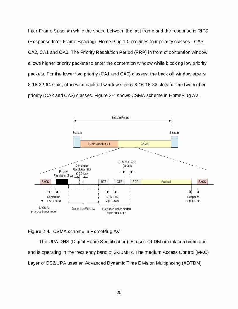
The CSMA access scheme in Home plug AV is the same as Home Plug 1.0 [15],
which is a modified CSMA/CA protocol with priority that allows Home Plug 1.0 stations
to communicate with each other without any centralized coordination. The space
between the last frame and the incoming frame is called CIFS (Contention Window
20
Inter-Frame Spacing) while the space between the last frame and the response is RIFS
(Response Inter-Frame Spacing). Home Plug 1.0 provides four priority classes - CA3,
CA2, CA1 and CA0. The Priority Resolution Period (PRP) in front of contention window
allows higher priority packets to enter the contention window while blocking low priority
packets. For the lower two priority (CA1 and CA0) classes, the back off window size is
8-16-32-64 slots, otherwise back off window size is 8-16-16-32 slots for the two higher
priority (CA2 and CA3) classes. Figure 2-4 shows CSMA scheme in HomePlug AV.
TDMA Session # 1 CSMA
Beacon
Payload SACKRTS CTS SOF
RTS-CTS Gap (100us)
CTS-SOF Gap (100us)
Only used under hidden node conditions
SACK
Contention IFS (100us)
Priority Resolution Slots
Contention Resolution Slot
(35.84us)
Contention WindowSACK for previous transmission
Beacon Period
Beacon
Response Gap (100us)
Figure 2-4. CSMA scheme in HomePlug AV
The UPA DHS (Digital Home Specification) [8] uses OFDM modulation technique
and is operating in the frequency band of 2-30MHz. The medium Access Control (MAC)
Layer of DS2/UPA uses an Advanced Dynamic Time Division Multiplexing (ADTDM)

21
scheme. This ADTDM scheme is essentially a centralized MAC protocol and supports
collision free access to PLC channel to all nodes in networks.
There is only master node in the network and this node controls channel access of
all other nodes by using a token packet. The Repeater can be placed in network to
forward the signal if the signal from master node cannot reach all slave nodes. The
slave nodes does not have the right to send any packets unless it is granted this right by
the master node.
Only one node has the right to transmit at any moment, however, the possibility of
duplicate tokens and token loss is not avoidable. Figure 2-5 illustrates this transmission
sequence of UPA/DHS.
Node A (Master Node)
Node B
Node C
Node D
Token for B Token for C Token for D
Token for A
Token for A
Token for A
RX/TX Switch Time : TokenTime
Figure 2-5. Transmission sequence of UPA/DHS
In Figure 2-5 node A starts the transmission process by sending data bursts to its
destination and gives the right to control the channel to node B by passing the Token
packet. After receiving the token from node A, node B starts transmission. After finishing
data transmission, node B returns the token to node A. The node A gives the token to
node C and D in order. Every slave node returns the token to node A after finishing data

22
transmission. If a node which has a right to control the channel does not have data to
send, this node immediately returns the token to node A.
The HD-PLC (High definition PLC) uses wavelet transform-based OFDM
(orthogonal Frequency Division Multiplexing) in the frequency band 4-28 MHz. This
wavelet OFDM uses 512 real carriers with symbol lengths of 8.192µs and the carriers
are modulated with PAM (Pulse Amplitude Modulation). HD-PLC devices can provide
maximum 190 Mbps of physical throughput or more without notches.
The MAC scheme of HD-PLC [9] uses a hybrid medium access protocol
composed of Time Division Multiple Access (TDMA) and Carrier Sense Multiple Access
(CSMA) in each beacon cycle. The architecture of the HD-PLC hybrid MAC is shown at
Figure 2-6.
TDMA CSMABeacon
1 Cycle
Figure 2-6. Hybrid Medium Access Protocol
In the TDMA region, a centralized channel access management is executed by a
central coordination node. The bandwidth schedule is announced to each node by a
beacon frame. Distributed channel access management is executed in the CSMA
region. In this region bandwidth is not guaranteed and the priority for each link in the
CSMA region is determined from the TOS (Type of Service) field in the IP header. If a
link has a high priority then a node has short Maximum Back off time.
Experiment Setup
The experiment was conducted in a 2200 square feet house in Gainesville, Florida.

23
The objective of this test was to determine the performance of recent PLC and wireless
technologies in a real world environment. The interior walls of this house are made of
wood and drywall. This can give a significant advantage for wireless technology’s
performance comparing to the same setup in a bricked or concrete wall environment.
Figure 2-7 shows the floor plan and the testing locations of this house.
Figure 2-7. Test floor plan
In this experiment, we used one desktop computer as a receiver and one laptop
computer as a transmitter. The desktop computer had a 3.0GHz Pentium IV processor
with 512 MB Ram and windows XP professional SP2. The laptop was equipped with a
1.87GHz Pentium IV processor, 512MB RAM and running on top of windows XP
professional SP2.
The software used for this test was Gatorbytes, a network throughput
measurement software developed by the University of Florida and Charleston Southern

24
University [16]. This program is able to provide real time data visualization that shows
the network status in real time. A snapshot of the Gatorbyte output screen is shown in
Figure 2-8.
Figure 2-8. Snapshot of Gatorbytes
Both TCP and UDP protocols are used in this test to evaluate the performance of
IEEE 802.11g/n and PLC technology. The TCP tests used 64240 byte segments while
1472 bytes packets were sent in the UDP tests. Each test lasts for 60 seconds. This test
gives us an idea of the optimal throughput of each technology. The setup for the PLC
tests are depicted in Figure 2-9, while the PLC adaptors used in the test are described
in Table 2-1.
Table 2-1. PLC Adaptors Model Name Maker Chipset Technology
RD 6300 Intellon Intellon Home Plug AV HDX101 Netgear DS-2 UPA-DHS BL-PA100 Panasonic Panasonic HD-PLC

25
HDX101 and BL-PA100 power line adapter used were the over the shelf products
while RD-6300 Homeplug AV power line adaptor is a reference design provided by
Intellon corporation.
Figure 2-9. PLC test configuration
An Ad-Hoc configuration was used in the wireless network experiments. The
configuration is shown in Figure 2-10.
Figure 2-10. IEEE 802.11g/n test configuration
The equipment used in the wireless experiments was Linksys, WUSB300N. Both
of the receiver’s and transmitter’s antenna were placed randomly and the
manufacturer’s default settings were used.
Test of UDP and TCP Protocol
The experiments were conducted in 18 paths with TCP and UDP protocols. All
PLC and IEEE 802.11g/n technologies have full whole house coverage in this test
meaning that there was some connection along every path tested. The Netgear’s PLC
adapter, HDX101 we used had the amateur radio tones turned on while the other PLC

26
adapters did not use the amateur radio bands. In the results presented, the HDX101
data rates are reduced by 20 % to correct for the amateur radio bands.
Figure 2-11. Link coverage versus TCP throughput
Figure 2-11 shows the percentage of links that exceed the TCP throughput value
noted at the X-axis. The experiment shows that Intellon’s PLC adapter RD 6300 has the
highest Maximum TCP performance. Figure 2-11 shows that around 77% of
connections operated at more than 47 Mbps. For the Netgear’s PLC adaptor, HDX101,
77% of the connections operated above 40 Mbps. For IEEE 802.11n ad hoc mode and
Panasonic’s PLC adapter BL-PA100, 77% of connection operated above 25 and 26
Mbps respectively. IEEE 802.11g ad hoc mode has lower TCP performance compared
with other products but gave the most stable output for wireless TCP performance.
15 20 25 30 35 40 45 50 55 60 650
10
20
30
40
50
60
70
80
90
100
Throughput (Mbps)
Link
Cov
erag
e(%
)
IntellonNetgaerPanasonic802.11g802.11n

27
Figure 2-12. Link coverage versus UDP throughput
Figure 2-12 shows the percentage of links that exceed the UDP throughput value
indicated on the x-axis. The Intellon’s PLC adapter RD 6300 has the highest maximum
and minimum UDP throughput. The minimum throughput of RD 6300 observed in the
experiment was 57.65 Mbps and 77% of connections operated above 64 Mbps. Notably,
this product had highest UDP throughput at all paths. For Netgear’s PLC adaptor,
HDX101, 77% of connections operated above 36 Mbps for UDP. But our experiment
revealed this product is vulnerable to be affected by interference.
As shown in Figure 2-12 the minimum throughput of HDX101 is 25.99 Mbps which
is an extremely low value compared with its maximum throughput. For the Panasonic
PLC adapter BL-PA100 and IEEE 802.11n in ad hoc mode, 77% of connections
operated above 36 and 42Mbps respectively. This experiment shows Maximum UDP
20 30 40 50 60 70 80 900
10
20
30
40
50
60
70
80
90
100
Throughput (Mbps)
Link
Cov
erag
e(%
)
IntellonNetgaerPanasonic802.11g802.11n

28
throughput of BL-PA100 is higher than that of IEEE 802.11n ad hoc mode but IEEE
802.11n has higher minimum throughput than that of Panasonic’s PLC adaptor BL-
PA100. IEEE802.11g ad hoc mode has lowest throughput as we know but again gave
the most stable throughput. The deviation of maximum and minimum UDP throughput is
just 1.07 Mbps. In this experiment the IEEE802.11g/n standards were operated as ad
hoc mode. We can expect that the throughput would be reduced to below half of our
test values for IEEE 802.11g/n operating in infrastructure mode which is normally used
in home and small area networks.
Figure 2-13. TCP throughput versus distance of direct path
The scatter plot of the TCP and UDP throughput as a function of distance is shown
in Figures 2-13 and 2-14. Normally wireless communication has direct relation between
distance and performance. But in this experiment we could not find any direct
15 20 25 30 35 40 45 50 55 60 6520
30
40
50
60
70
80
90
Thr
ough
put (
Mbp
s)
Distance (ft)
IntellonNetgaerPanasonic802.11g802.11n

29
relationship between distance and throughput. Especially IEEE 802.11g has almost the
same performance irrespective of path distance. The performances of PLC systems
have no correlation with the line of sight distance measure in this experiment. This is
because PLC signals are transmitted through the convoluted power network cables
which reach the destination.
Figure 2-14. UDP throughput versus distance of direct path
HDTV Streaming Test
To assess the feasibility of the distribution of a single HDTV stream in the home, a
25Mbps HDTV stream was transmitted and received using each of the technologies
studied. In this experiment we made a connection between the laptop and the desktop
computer using PLC and IEEE 802.11g/n technologies and the HDTV stream was
played over the power line and wireless network using the PowerDVD multimedia player.
15 20 25 30 35 40 45 50 55 60 6515
20
25
30
35
40
45
50
55
60
65
Thr
ough
put (
Mbp
s)
Distance (ft)
IntellonNetgaerPanasonic802.11g802.11n

30
A momentary video freeze phenomenon during playback occurred if the overall bit rate
of the videofile was close to or exceeded the capacity the path for the selected
technology. We conducted this evaluation on 5 paths in the same house. Table 2-3
shows the quality evolution for HDTV streaming. We evaluated the quality of video
streaming in 4 categories of an informal Mean Opinion Score (MOS): “4=Very Good”,
“3=Good”, “2=Poor” and “1-Very Poor. Table 2-2 shows the classifications used.
Table 2-2. Classification of video streaming Classification Playback condition
4 Very Good: Video streaming is smooth and no packet drop is observed. Or it is hard to realize the packet drop
3 Good: video streaming has slight discontinuity or delay
2 Poor: Video streaming has evident discontinuity or delay but delay is not significant
1 Very Poor: video streaming has serious discontinuity and delay so quality of video is not tolerable.
Table 2-3. Quality of 25Mbps, HD video streaming Product Path 1 Path2 Path3 Path4 Path5 Avg. Intellon RD6300 3 4 2 2 3 2.8 Netgear HDX101 2 1 2 3 2 2 Panasonic BL-PA100 1 2 1 1 1 1.2 Linksys 802.11G 1 1 1 1 1 1 Linksys 802.11N 1 1 1 1 1 1
In the experiment with MPEG-2 file with a bit rate of 25Mbps, we observed a
serious video freeze and go (halting) phenomenon with IEEE 802.11g and n technology.
The delay of IEEE 802.11g is more serious than that of IEEE802.11n. Panasonic’s BL-
PA100 PLC adaptor also shows bad video quality. Intellon’s RD6300 and Netger’s
HDX101 PLC adaptor shows better performance than other technologies as we
expected. But these could not support a 25 Mbps HD video signal successfully at all

31
paths. (Note: the Negrear HDX101 adapters had the amateur bands turned on for these
tests).
Conclusion
This study presents a comprehensive evaluation of the performance of recent
wireless and PLC technologies for home and small office environments. The throughput
of IEEE 802.11 g/n and High speed PLC technologies in a real world environment was
measured. The experiments were conducted along 18 paths with TCP and UDP
protocols in 2200 square feet house. HDTV streaming was also evaluated over five
paths. All power line and wireless technologies tested in our experiment provide full
connectivity with each other.
Our overall experimental results shows the Homeplug AV PLC adapter
outperforms other PLC products and the IEEE802.11n/g for UDP and TCP throughput
and HDTV streaming performance.
The work reported in this chapter has been published in the Proceedings of 12th
World Multi-Conference on Systemics, Cybernetics and Informatics (WMSCI2008) [33].

32
CHAPTER 3 A VISUALIZATION TOOL FOR NETWORKING PROTOCOL ANALYSIS
Introduction
Recent decades have seen exponential increase in the amount of digital
information flowing across data networks. Digital information goes through several
network layers before reaching the intended destination. Each network layer deals with
a specific facet of the networking problem. For example, the IP layer is responsible for
proper routing while the physical layer deals with the transmission and reception of
signals over the medium. Network layers implement a set of protocols or behavior rules
that enable them to perform their intended function. Finite State Machines (FSM’s) are
widely used in modeling and implementation of networking protocols. Typically these
FSM’s are augmented by means of variables and state transition dependencies based
on their values. For example, the modeling of the widely used TCP protocol will include
such states as the Slow Start, Congestion Avoidance and variables such as the
duplicate acknowledgments counter used for modeling the fast retransmission and fast
recovery protocol.
The current generation of networking protocols and hence the FSMs that are used
to implement them can are quite complex. Analytical tractability of their behavior is
limited to a very small subset of their range of behavior. Network engineers typically use
simulations for developing and enhancing the protocols. These simulations output
various statistics that can be used to estimate and improve system performance.
Several types of statistics can be collected from a simulation based on the parameters
of interest. Aggregate statistics provide information over the whole duration of the
simulation and hence describe the average system behavior. Dynamic behavior of the

33
system can be captured by means of windowed statistics (i.e., statistics generated over
a widow of time) or by means of the detailed trace file. Special events can be captured
by means of log files containing the relevant event information such as the time of
occurrence, event type, outcome, etc. Typical system/simulation performance
verification is accomplished by comparing the system behavior to the expected
behavior.
Recently, there has also been an increasing trend to support Quality of Service
(QoS) for multimedia streaming both within the Small Office/ Home Office (SOHO)
environment as well as more generally over the Interne. There has also been an
increasing need for designing intelligent protocols that automatically adjust to changes
in network conditions based on cross layer information. Networking protocols required
to support such functionality are significantly more complex than the current generation
of protocols. The design and verification of such protocols can leverage the statistics
gathered from the simulations. However, in several instances it becomes important to
go through a long trace file to understand the behavior of the system under certain
events.
One such example is the design of contention based medium access control
protocols like the CSMA/CA protocol used in IEEE 802.11 Distributed Coordinated
Function and in the Powerline HomePlug 1.0 MAC. In CSMA/CA networks, multiple
stations use a combination of carrier sensing and back-off algorithm to obtain medium
access. Collisions are common in such networks and optimal performance is typically
obtained by balancing the collision costs with the time wasted due to idle contention
slots. To verify the proper operation of such protocol, one has to go through in detail the

34
trace files of the states of various stations as a function of time, including their internal
variables and check if they behave as expected. However, going through a long trace of
data is cumbersome and error prone.
To overcome this problem we developed a new Visual Protocol Analyzer named
EVGATOR [17] that can juxtapose and plot states of multiple FSMs as a function of
time. This utility is configurable so that each state of the FSM is represented by a
specific color. The EVGATOR tool proved to be of great advantage in analyzing the new
network high speed Powerline protocols.
Requirements
In a generic network protocol simulation, there are multiple instantiations of nodes
with each node modeled using a set of FSMs. A subset of state traces of these FSMs at
each node can be of interest. Assume there are j nodes on the network and that each
node has k FSMs represented as
FSM[1]_State, FSM[2]_State, …… , FSM[k]_State
Each FSM contains mi states that can be denoted by
FSM[i][1]_State, FSM[i][2]_State, …, FSM[i][mi]_State.
where i represents the ith FSM. At any time, each FSM[i] State contains only one of the
mi available states of the ith FSM. Thus, the general format of the trace file information
is,
Time,Node[1]_States Vec,…,Node[j]_States Vec
where, Node[j] States Vec is a state vector containing the state of each of the k FSM’s at
Node j.

35
Since the set of states for a given FSM is simulation dependent, the FSM state
plotter should be easily configurable to any set of states. Further, the number of Nodes,
j, and the number of FSM’s per Node, k, and the number of states of each FSM, mi,
should also be easily to configure.
Apart from these, the following features will be useful to have in the FSM state
Plotter,
• Ability to choose the color/texture by which each of the states is displayed,
• Ability to dynamically turn on and off the states that need to be displayed,
• Ability to change the size of time window that is displayed and easy means of
zooming in and out of the region of interest,
• Ability to jump to a certain point in time, and
• Ability to print and copy the display region.
EVGator has all the above features. Note that in practice, depending on the way
the simulation is designed, it may not be possible to generate a single trace file
containing data from all the FSM’s. For example, each instantiation of an FSM may
independently generate its trace file. In such cases, it would be necessary to preprocess
the respective data files to generate a single file containing all the data which could then
be analyzed by EVGATOR.
Design and Implementation
The EVGATOR tool was developed using Microsoft Visual Studio .Net platform.
The programming language we used was Visual C++, largely due to its wide
acceptance in industry and academia. The EVGATOR is an event driven program and
thus it reacts only when user commands or system events trigger the associate
functions. For example, EVGATOR remains idle until the OS sends a mouse event to it.

36
The mouse event is then recognized by the gesture recognition function, which then
triggers a window re-draw event to the OS to reflect the corresponding mouse gesture.
The OS sends mouse events only when the mouse cursor is in the EVGATOR client
window and the EVGATOR is the current active window.
Design of the EVGator User Interface
Humans are more sensitive and responsive to graphical data than to text.
Especially when analyzing complex situations, people usually use drawings to help
themselves to reason. For example, Figure 3-1 shows two modes of the same event
transition in a simulation output. People can easily understand the state transition
displayed as a rather than the textual description of the same event shown on the
figure. This comparison gives us a clear indication of the need of a visual protocol
analysis tool - EVGATOR. To meet the requirements, EVGATOR contains the following
features:
• Ease and efficiency in communicating with the analyzer.
The manner in which an operator interacts with the analyzer dictates the efficiency
and ease of analyzing a simulation result. We choose to use mouse cursor as the major
User Interface (UI) for the following reasons. First, using the mouse cursor is an intuitive
way of interacting with modern operating systems and people are already familiar with
mouse operation. Secondly, using mouse is more effective if the User Interface (UI) is
reasonably designed.
However, we did not completely abandon the usage of a keyboard. It is undeniable
that under some circumstances the keyboard is more efficient than mouse operations.
For example, to jump to a specific time stamp (if the value of the time stamp is known)

37
the operator simply needs to type the value into an edit box and that would be faster
than using mouse to browse to the desired time mark.
• Ease to range magnification and contraction (Zoom).
Figure 3-1. Text versus graphical event analyzer
Some events rarely happen except when simulated for a certain amount of time.
Thus usually protocol designers will often simulate a scenario for a long time in order to

38
find out the possible design flaws. In this case, the time line in the analyzer could
become quite lengthy. Thus an analyzer should be able to zoom into a specific time
frame to reveal detailed protocol state transition in that time range. It also should have
the ability to zoom out to display a global view of the state transitions to find out the
correlations between events.
To achieve this goal, we designed mouse gestures to represent zoom in and out.
Designers can use the mouse to mark a range of time which represents the time frame
for operation. If designers click within the range, then the analyzer assumes it is a
command of ”Zoom In”. Otherwise it will zoom out so that the marked time frame
occupies half of the window. Designers can easily mark various lengths of time frames
to achieve various zoom factors.
If designers want a specific zoom factor, they can also use the keyboard to type
the value into the zoom factor edit box. To prevent ambiguity, the marked time frame is
also shown as a text display on the display window.
• Ease of marking a specific time.
When examining simulation results, designers usually have to look at various time
stamps to understand the causes of aberrant events. Without the mark function, it would
be difficult to move back and forth between time frames.
In the EVGATOR system, designers can achieve this effect by simply clicking on
the display window. To help designers understand the marked time, the EVGATOR also
shows the marked time value in the display window.
• Ease of navigation throughout the whole time line.

39
Since the simulation results are usually large, a display window width is not able to
display all events at a time. To improve the quality of the event browsing experience, we
use scroll bars to travel between time frames. Since scroll bars are elastic to the mouse
movements, designers can drastically move the mouse to achieve large step jumps or
click on the end arrow box to achieve small scale time line adjustments, either forward
or backward.
• Flexibility in changing both event display colors and event names.
Since humans are sensitive to colors, EVGATOR displays different events with
different colors. Meanwhile, different protocol designs may have different event naming
and thus the EVGATOR is elastic enough to adapt to these minor changes without
recompiling the source code.
To achieve the above goals, EVGATOR reads a configuration file before it starts to
parse log files. Designers can modify the configuration file to suit their needs. For
example, if a protocol has a new state called “Preparation”, designers can open the
configuration file using a text editor, and add a new line of the event name and the
associated representing color. The EVGATOR will automatically add the new event into
its control panel and in the representing diagram. The EVGATOR is not only elastic to
the offline event representing modifications, but it is also adaptive to real time changes
as well. For example, if designers are looking for a specific event, they can turn off other
events to make the desired event stand out in the final diagram as shown in the Figure
3-2. The above mentioned EVGATOR features makes using EVGATOR for analyzing
protocol events efficient and easy. It can also significantly reduce the time required to
debug a simulator.

40
Figure 3-2. Example of selecting desired events.
Configuring the EVGATOR
As we mentioned earlier, the EVGATOR requires a configuration file for state
presentations. The example is shown in Figure 3-3.
The first line in shows a state name: INITIALIZATION and the second line shows
the color that represents this event. Each statement occupies one line. EVGATOR
supports 100 different states and 255 nodes. Users do not have to specify the total
number of states in the configuration file. EVGATOR will determine the effective state
names and number of states.
Trace File Format
To translate text log files into diagram forms, EVGATOR has to parse the recorded
information. The sample log file format is shown in Figure 3-4.

41
Figure 3-3. EVGATOR configuration format
Figure 3-4. Generated trace log file format
The tokens are defined in the configuration file. When EVGATOR sees a text
string that is equal to a token, the index of the token is stored into an internal state
queue associated with the starting time stamps. If a text is not recognizable during
parsing, the EVGATOR will skip that text. The EVGATOR will keep parsing every text

42
string in the log file until the end of the file. When a token is recognized, the ending time
stamp of the previous state is also decided.
After a whole file is parsed, the EVGATOR will start to display each state with the
colors defined in the configuration file. Since the window height and width is limited and
is usually smaller than the simulation duration, the real data displayed is a small portion
of the whole data as shown in the Fig. 3-5. To help designers browse, a ”Zoom In” and
”Zoom Out” command is required.
Zoom – In/Out
To implement ”Zoom In” and ”Zoom Out”, we need to calculate the Zoom Factor.
Initially the Zoom Factor is defined as one. Before calculating the zoom factor, the
EVGATOR first translates the marked time frame to coordinates of the display. The
translation can be done by Eq.3.1
M1 = (Mark_ Time1 –Min_ time) ×Zoom_ Factor
M2 = (Mark_ Time2 –Min_ time) ×Zoom_ Factor (3.1)
Figure 3-5. Example of actual display window
If the mouse gesture is a “Zoom In” command, that is, the user makes a mouse click
within the marked time frame, the zoom factor can be calculated by dividing the current
display time frame with the marked time frame as shown in Eq. 3.2.

43
2 1
1 2
x - xZoom_Factor = M -M (3.2)
If the command is a “Zoom Out”, the zoom factor is calculated by dividing the
marked time frame with the current display time frame as shown in Eq. 3.3.
1 2
2 1
M -MZoom_Factor = x -x (3.3)
Since the simulation log file is huge, we need a proper data structure to represent
state transitions. An event queue is used in EVGATOR. The queue is dynamically
allocated and de-allocated in order to minimize the system memory requirement.
To reduce window flickering due to the updating of display contents, we record the
areas that are affected by the current operation and update those areas only. This way,
only a small portion of the display areas needs to be updated at a time.
Experience
The EVGATOR utility was very useful to us in developing the Medium Access
Control protocol of HomePlug AV, which is intended to be the successor to the
HomePlug 1.0 Standard [15]. During the development and analysis, we made extensive
use of the EVGATOR functions described above.
EVGATOR was particularly useful in the verification of the simulation and in
understanding some of the rare/unexpected events that occurred. In the former case,
the visual plot of the MAC and Physical Layer state as a function of time proved to be a
valuable tool in trying to find any erroneous behavior. In the later case, when an
unexpected and very rare event happened, the GUI helped us to quickly go through the
set of events that caused the final event. For example, in the process of designing the
CSMA/CA protocol, we found that searching for the causes of nodes moving to the

44
back-off state using the text based log file is painful since there are so many different
state transitions occurring at the same time. However, using EVGATOR we can easily
find the cause using the displayed diagram. In Figure 3-2, we found the cause of the
back-off is because of the RTS collisions.
Conclusion
With the help of the EVGATOR, we significantly reduced the protocol design
process and the time spent on debugging the simulation results. Designers who work on
FSM-based simulators can also benefit from the visualized expressions of state
transitions. Though EVGATOR is helpful, it cannot directly parse trace logs from other
simulators like NS-2 or Opnet. However, users can readily transform the given log
formats to the format EVGATOR accepts. We also expect the inputs from industry and
academia to help us keeps developing and improving EVGATOR to meet majority of
users’ needs, possibly with automatic data format conversion of the most popular
simulation environments.
EVGATOR is now available on UF LIST website
(http://www.list.ufl.edu/VisuGATOR) as a public domain freeware, with some required
rights held by the University of Florida to the present source code.
The work reported in this chapter has been published in the International Journal
of Software Engineering and Its Applications [17].

45
CHAPTER 4 ENHANCED LIMITED ROUND ROBIN MECHANISM USING PRIORITY POLICY
OVER BLUETOOTH NETWORK
Introduction
The smallest Bluetooth unit is called a piconet, which is composed of one master
node and several slave nodes (up to seven).In a piconet a Bluetooth device can be
operate in active mode or sleep mode (Sniff, Hold and park mode). However just one
master and seven active mode slaves are allowed in a piconet. If some nodes desire to
switch the state to active mode, some active nodes should change the state from active
mode to sleep mode when seven slaves are already operated in active mode. All nodes
in a same piconet should follow same frequency hopping pattern. Multiple piconets can
also exist in the same area and be connected via a bridge node, creating a scatternet.
In a Bluetooth system, full-duplex transmission is supported using a master-driven
TDD (Time Division Duplex) scheme to segment the channel into 625µs time slots,
which are alternatively distributed between the master and the slaves. As such, the
master sends a poll or data packet to a slave using the even-numbered slots, then the
slave sends a packet to the master using an odd-numbered slot immediately after
receiving a packet from the master [4]. Thus, the MAC scheduling in Bluetooth is
controlled by the master and executed using master-slave pairs. All Bluetooth devices in
a same piconet have to synchronize the clocking exactly and a node which has privilege
of using the slot will not release the resource of transmission to other nodes even if it
does not have any data to transmit. Hence Bluetooth seems to be inefficient but it can
support more reliable connection. So Bluetooth is appropriate for high quality
interconnection between mobile devices and many researchers have proposed
algorithms to enhance the performance of Bluetooth network [18-22].

46
Bluetooth systems support two types of virtual data communication link between
the master and slave: a Synchronous Connection Oriented (SCO) link and
Asynchronous Connection-Less (ACL) link. An SCO connection supports a circuit-
oriented service with a constant bandwidth using a fixed and periodic allocation of slots.
An SCO connection is suitable for latency-sensitive multimedia traffic like voice traffic,
whereas an ACL connection supports a packet-oriented service between the master
and slave for data. An SCO connection only uses one time slot, while an ACL
connection can use one, three, or five time slots according to the data packet size [4].
The Round Robin (RR) scheme is a default MAC scheduling algorithm for Bluetooth that
uses a fixed cyclic order. The POLL packet does not have any information and just
gives the polled slave the privilege of transmitting packet in next slot. If the polled slave
does not have any data to transmit, it replies to the master by sending a NULL packet
which also does not have any information. As a result, numerous slots can be wasted
with POLL or NULL packet exchanges in the case of no data to transmit. Despite the
introduction of several Bluetooth MAC scheduling algorithms to reduce these slot waste,
problems still remain.
Accordingly, this section introduces a simple and efficient MAC scheduling
algorithm to reduce slot waste and enhance the performance of Bluetooth.
MAC scheduling scheme of Bluetooth
The principal MAC protocol in Bluetooth is a polling scheme that uses a master-
driven time division duplex (TDD). Here, a slave is only allowed to transmit a packet to
the master immediately after receiving a packet from the master. Plus, the master can
only use an even-numbered slot to send a packet to a slave, while the slave can only
reply to this packet using an odd-numbered slot. The MAC scheduling scheme for a

47
Bluetooth system is shown in Figure 4-1. The TDD slots are shared by the SCO and
ACL link in this figure.
Figure 4-1. MAC Scheduling scheme of Bluetooth
In the Pure Round Robin (PRR) scheme, every slave has the same opportunity to
send one data packet even when they have no packet to transmit. Once the master
polls a slave, the next time slot is then assigned to the slave without reference to
whether the slave has data to transmit or not. Consequently, numerous slots can be
wasted when POLL packets are sent by the master and NULL packets are sent by the
slaves in the case of no data packets to transmit. Therefore, the PRR scheme is an
inefficient scheduling algorithm when the traffic in the network is asymmetric, and
several Bluetooth MAC scheduling algorithms have already been proposed to improve
the system performance [18-22]. Some works assume that the Master knows up-to-
date information of slave’s queue status [18-20]. Some approaches do not require this
information [22]. Some researchers also proposed low power mode based scheduling
policy [21].
In [18], a Master-Slave Queue-State-dependent Packet scheduling algorithm is
proposed, where a free bit in the Bluetooth payload header is used by a slave to inform

48
the master of the next available data. Based on this feedback bit, the master classifies
all the master-slave pairs into one of four states, and a higher priority assigned to a pair
that utilizes the slots more efficiently than the other pairs. However, this algorithm
assumes that the master has updated information on the slave queue at all times, which
is not actually available given the current Bluetooth specifications, as the slaves can
only provide information on their queue state when they send a packet to the master. In
addition, a slave starvation problem can occur for low priority pairs when higher priority
pairs always have packets to transmit.
In [19], HOL-Priority Policy (HOL-PP) is proposed. This algorithm use similar
priority policy with [18]. The master schedules on the basis of the head of line (HOL)
packet size at the Master and slave queue. Additional two bits are required to
distinguish 4 possible HOL packet size for classifying the master and slave pair into
three classes by slot utilization. However this policy assumes the master has up-to-date
information of slave queue’s status like [18].
In [20], the authors use the similar priority policy as in [18] and [19] to improve the
performance of the system considering both throughput and delay on each Master-
Slave pair in scheduling decision. They use the amount of link utilization to assign a
priority class based on queue status of master and slave pairs. But they also assume
that the master knows up-to-date information of the slave-to-master queue status.
Some researchers proposed MAC scheduling policy to optimize power
consumption and improve slot utilization by using a low power mode in Bluetooth [21].
In this research authors proposed variable sniff interval and variable serving time on the

49
base of slot utilization. However this scheduling policy is not adequate for dynamic
traffic and requires additional information.
In [22], several scheduling algorithms are compared. The Exhaustive Round
Robin (ERR) is a simple scheduling policy that uses a fixed order like RR. Yet, since the
master does not switch to the next slave until both the master and the slave queues are
empty, there is a danger that the channel can be captured by stations generating a
higher traffic than the system capacity. Thus, the Limited Round Robin (LRR) was
proposed to solve this capture effect Although the LRR also has a fixed cyclic order and
is exhaustive, like the ERR, parameter “t” is adopted to limit the number of
transmissions (tokens) that can be performed by each pair per cycle. The maximum
number of transmissions per cycle then limits the cycle length and avoids the capture
effect. Nonetheless, despite an improved throughput and fairness when compared with
the RR and ERR, the LRR still suffers from a slot wastage problem under asymmetric
traffic conditions.
Accordingly, on the foundation of the MAC scheduling algorithms in [18] and [22],
this section introduces an Enhanced Limited Round Robin with a priority policy (ELRR-
PP) based on slot utilization to improve the performance. Plus, fairness is maintained
using a maximum number of transmissions per cycle.
ELRR-PP Algorithm
The ELRR-PP [23] operates in accordance with the master-slave queue status. As
such, four classes of priority are assigned to the master-slave pairs based on the
existence of data in the respective queues, which is similar to the method in [18], except
the proposed method uses the current queue status for the master and previous queue
status for the slave.

50
Table 4-1. Priority Scheme Priority Queue status
Class 1 Master has packets in queue and the slave sent packets to the master during previous turn
Class 2 Master has packets in queue and slave did not send packets to the master during previous turn
Class 3 Master has no packets in queue and slave sent packets to the master during previous turn
Class 4 Master has no packets in queue and slave did not send packets to the master during previous turn
Hence, additional information on the slave queue is not necessary, in contrast to
[18]. This priority scheme is described in Table 4-1. Based on the classes, the slave
with the highest priority is polled first. It is also assumed that class 2 has priority over
class 3, as there is a possibility that the slave has no data to send to the master In the
case of several pairs in the same class, the pair with the largest amount of data in the
master queue has priority. But for the class 2, the pair with the smallest amount of data
in the master queue has priority to relegate this pair to class 4. The ELRR-PP algorithm
is described in Figure 4-2.
To avoid starvation of the low priority pairs, a maximum number of transmissions
per cycle is adopted for each class, where Max1 is the maximum transmission number
for class 1, and Max2, which is smaller than Max1, is the maximum transmission
number for class 2 and class 3. Parameter “t” is used to count the number of
transmissions. To prevent slot waste, the polling interval for class 4 pairs is modified.
For the first cycle, such an inactive pair has the same opportunity to be polled. But, if it
still has no packets to send in the next cycle, the polling interval for this pair is increased

51
linearly by one cycle to limit the chances of transmitting packets. Parameter “i” is used
for this purpose in Figure 4-2.
Figure 4-2. Flow chart of ELRR-PP
Performance Evaluation
To evaluate the proposed algorithm, a discrete event simulator was used, and all
the simulations were based on a single piconet consisting of one master and six slaves,

52
where the master had a corresponding queue for each slave. The traffic mode
considered was ACL. The traffic at the master and each slave was generated
independently in accordance with a Poisson process. When comparing the proposed
algorithm with other algorithms, the maximum number of transmissions per cycle for the
LRR was set at 4, while for the proposed ELRR-PP it was set at 8 for class 1(Max1=8)
and 4 for class 2 and class 3 (Max2=4).
Figure 4-3 shows the average delay when each master-slave pair had the same
arrival rate. As shown in Figure 4-3, the ELRR-PP produced a lower delay, however, the
difference compared to the other algorithms was not significant.
Figure 4-3. Average delay with same arrival rate
To evaluate the delay characteristics when each pair had a different traffic
generation rate, the arrival rate was changed, as shown in Table 4-2. The arrival rate of
the 6th master-slave pair was changed from 0.03 to 0.27 to increase the system traffic

53
from 0.4 to 0.88. As such, the arrival rate for slave 6 was increased from 0.03 to 0.27,
while that for the master was selected randomly between 0.03 and 0.27.
Table 4-2. Traffic Generation Parameter
Piconet M1 S1 M2 S2 M3 S3
Arrival rate 0.2 0.02 0.05 0.007 0.007 0.05
Piconet M4 S4 M5 S5 M6 S3
Arrival rate 0.001 0.002 0.002 0.001 Variable Variable
Figure 4-4. Throughput with variant traffic load
Figure 4-4 presents the throughput for the 6th master-slave pair with a variant
traffic load. As Expected, the PRR produced a lower throughput than the other
algorithms due to the increased traffic load for slave 6. Meanwhile, the ELRR-PP
produced a higher throughput than the LRR, and higher or similar throughput to the
ERR.
54
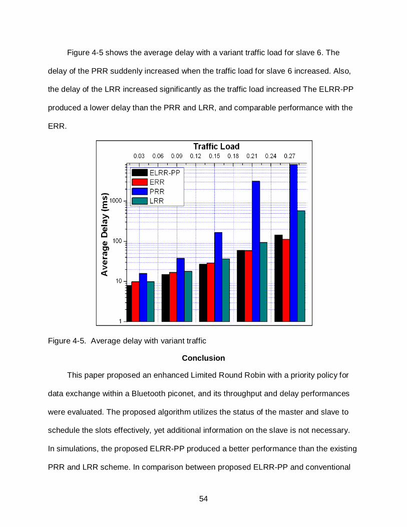
Figure 4-5 shows the average delay with a variant traffic load for slave 6. The
delay of the PRR suddenly increased when the traffic load for slave 6 increased. Also,
the delay of the LRR increased significantly as the traffic load increased The ELRR-PP
produced a lower delay than the PRR and LRR, and comparable performance with the
ERR.
Figure 4-5. Average delay with variant traffic
Conclusion
This paper proposed an enhanced Limited Round Robin with a priority policy for
data exchange within a Bluetooth piconet, and its throughput and delay performances
were evaluated. The proposed algorithm utilizes the status of the master and slave to
schedule the slots effectively, yet additional information on the slave is not necessary.
In simulations, the proposed ELRR-PP produced a better performance than the existing
PRR and LRR scheme. In comparison between proposed ELRR-PP and conventional

55
ERR, our proposed ELRR-PP has better or comparable performance when the ERR is
vulnerable to a channel capture problems. The work reported in this chapter has been
published in the International journal of Advanced Science and Technology [23].

56
CHAPTER 5 EFFICIENT MOBILITY MANAGEMENT SCHEME OVER WIRELESS LOCAL AREA
NETWORK
Introduction
While wireless local area network (WLAN) has been designed and utilized for
small area application with limited mobility support, WLAN is gaining attention to support
high speed wireless service for wide hotspot area as a part of mobile cellular network
such as Universal Mobile Telecommunication system (UMTS) and General packet
Radio Service (GPRS) or an independent system.
The mobile Node (MN) can move around among Access Points (AP) which are in
the same network without losing current connection because the IEEE 802.11 standard
provides a link layer roaming. This process of link layer switch is called L2 hand over
and has AP probe, authentication and association phases in IEEE 802.11 based WLAN.
However the IEEE 802.11 standard cannot support MN’s continuous communication
with AP at every time for public user since there are many separate networks which
have a unique IP address in wider hot spot area. If the MN moves to an AP which is not
in a same network it has to reconfigure its IP address again which makes current
connection becomes disabled.
The Mobile Internet Protocol (MIP) supports IP level mobility to provide
seamless connectivity to MNs when it moves to another AP which is in a different
subnet. The MIPv6 [11] was proposed by the mobile IP working group in Internet
Engineering Task Force (IETF) to manage movement of MNs in wireless IPv6 network.
In MIPv6 protocol, IP level mobility is provided by binding a Home of Address (HoA) and
Care-of Address (CoA) at a Home Agent (HA) and Correspondent Node (CN). When a
MN moves to a new Access Router (AR) in different subnet it should obtain a CoA using

57
Router Advertisement (RA) message from the new AR which is Foreign Agent (FA) in
this case and notifies this CoA to the HA and CN to bind the CoA and HoA.
This procedure of network layer switch is called a L3 handover. Packets sent to
the MN cannot be delivered until the binding CoA and HoA is finished at HA. So this
disruption may degrade the quality of service especially for real time and delay sensitive
traffic such as a multimedia streaming and voice over IP (VoIP) service. To improve the
handover performance of MIPv6 several schemes have been proposed such as Fast
Handover for Mobile IPv6 [12]. To provide the MN’s mobility in IPv6 network, the
protocol stack of MN is required to be modified for supporting the MIPv6. This
modification is too complex considering with limited capacity of the MN and participation
of MN in mobility signaling causes increase of power consumption of the MN.
The proxy Mobile IPv6 (PMIPv6) [14] is a network based localized mobility
management (NetLMM) protocol which has been proposed by IETF NetLMM working
group. In this PMIPv6 the modification of MN’s protocol stack is not necessary and MN
is not involved in IP mobility related signaling. On behalf of the MN, the network is liable
for managing IP mobility. The PMIPv6 guarantees the localized mobility support of MN
when MN roams within a local mobility domain region.
Enhanced Handover Scheme of MIPv6 with Fast Movement Detection & DAD
Overview of MobileIPv6 (MIPv6)
The Mobile IPv6 (MIPv6)[11] is a host based mobility management protocol to
support global mobility of the MN. The MN uses a permanent HoA and temporary CoA
in the MIPv6 protocol. When the MN enters a foreign domain the MN should obtain the
new CoA from router advertisement message. After configuration of new CoA
Duplicate Address Detection (DAD) procedure is performed. Then the MN registers

58
this CoA with the HA through binding update (BU) message. When the MN moves
away from home network the HA works as a stationary proxy.
NARPAR HA
Binding Update (New CoA)
MN CN
Packet
L2 Establishment
Rendezvous Time
Registration to HA
Periodic Unsolicited Router Advertisement
Router Solicitation
Router Advertisement
CoA Configuration and DAD (upto 1000ms)
Binding Acknowledgement
Packet
Figure 5-1. Mobile IPv6 handover procedure
The HA intercepts packets destined to the HoA of the MN and forwards these
packet by tunnelling to the CoA of the MN. For efficient transmission of packets the
Mobile IPv6 has a route optimization scheme. In this scheme the MN sends its new CoA
to CN by BU message. After receiving this BU message the CN sends packets to the

59
MN directly. However packets from CN are delivered to the MN via the HA until the CN
receives the new CoA of the MN. Figure 5-1 shows handover procedure of mobile IPv6.
The MIPv6 handover procedure consists of movement detection, new CoA
configuration and location update. These procedures cause a long handover latency
which can not acceptable for real time multimedia application. In order to improve the
handover latency the various extensions of MIPv6 such as fast handover for Mobile
IPv6 (FMIPv6) [12] and hierarchical MIPv6 (HMIPv6) [13] have been proposed. Though
a lot of enhanced MIPv6 schemes have been reported over the past year the MIPv6 has
not deployed widely in practice because of heavy specification which has to be
implemented at small mobile node for supporting MIPv6.
Movement Detection Procedure in MIPv6. The primary aim of movement
detection is to identify L3 handovers. In MIPv6, movement detection generally uses
Neighbor Unreachability Detection to determine when the default router is no longer bi-
directionally reachable, in which case an MN must discover a new default router on a
new link.
However, this detection only occurs when the MN has packets to send, and in the
absence of frequent router advertisements or indications from the link-layer, the MN
might become unaware of an L3 handover. After a change of link layer connection the
MN must detect any change at the IP layer before it can signal the change to the
network. MIPv6 uses RS and RA to detect changes of IP network prefix. This is part of
the standard router discovery protocol.
The protocol contains built-in timers, these timers prevent a router from sending
immediate responses to RS in order to prevent multiple nodes from transmitting at

60
exactly the same time and to avoid long-range periodic transmissions from
synchronizing with each other. These are the significant delays since they interfere with
the MIPv6 movement detection algorithm thus preventing mobility signaling for up to
1000ms [11].
Proposed MIPv6 Handover Scheme with FMDD
NAR PAR HA
Binding Update (New CoA)
MN NAP
Stored RALink layer establishment
Registration to HA
New Router Solicitation
New Router Advertisement
Binding Acknowledgement
Packet
L2 Association Response
L2 Association Request
RA message
Lookup delay for DAD
Rendezvous Time
Figure 5-2. Mobile IPv6 handover procedure with FMDD Scheme
Most handover mechanisms for MIPv6 make use of movement detection
algorithms, which use received RA information and configuration of new CoA. However,
61
in movement detection, RS delays the transmission for a random amount of time [6].
This time serves to alleviate congestion when many hosts start up on a link at the same
time. Also, RA must be delayed by a random amount time. In DAD procedure, after
generation of the CoA, an MN has to check CoA’s uniqueness [39] [40].
The duration required to complete DAD is up to 1 second. These delays for RS,
RA, and DAD are inherent to MIPv6. In this section, we illustrate our proposed fast
movement detection and duplicate address detection mechanism for fast handover in
MIPv6. Figure 5-2 shows the MIPv6 handover procedure with fast movement detection
& DAD (FMDD) scheme.
Movement Detection using Stored RA message
For movement detection, the MN performs a scan to see APs through probes. The
result of the scan is a list of AP’s information. Authentication is performed, and then the
MN sends the (Re) association request message with its MAC address. The AP grants
association by sending the Association Response Message. As soon as association is
made, the AP sends Stored RA (SRA) to an MN with MAC address in Association
Response message [38]. However, in our proposed Movement Detection scheme, when
the MN receives the SRA message from an AP during an L2 handover, the MN
compares the prefix of the RA message with existing own prefixes in the cache. If the
prefix is different, the MN can generate a new care of address (CoA) using the stateless
address auto-configuration method and the prefix option allowed in RA messages.
Before finishing an L2 handover, the MN sends the RS message by unicast to the new
AR using the received SRA’s source address included in the Association Response
Message. “Unicast” is of great significance since it can reduce the network load and
avoid the Random delays attributed to RS and RA.

62
An MN is able to help smooth proxy handover by adding the new CoA generated
by an MN to the RS as an option to provide interoperability with normal nodes. This
happens by using a bit in reserved field and notifying the node that follows by the
scheme that we offer. We name this bit as the New MN (NMN) and the two options as
Previous MN’s CoA and previous AR’s global address. This modified new RS message
is also named as NRS. When the new AR receives the NRS message from an MN, the
AR performs DAD as well as movement detection by using the neighbor cache.
DAD configuration and Lookup Algorithm
The proposed DAD method is to use of the neighbor cache of an Access Router
(AR) with sufficient buffer size to allow many nodes to attach simultaneously. Firstly, the
MN allocates this generated New CoA in its interface without DAD. We need to consider
how a neighbor cache and the Neighbor Unreachability Detection procedure perform
DAD. As stated [39], a neighbor cache contains one entry for each neighbor to which
the node has recently sent messages. Each entry of a neighbor cache may be
generated by the RS, the Neighbor Solicitation (NS) or the Unsolicited Neighbor
Advertisement (NA) in the case of router. The entries generated in this way are
maintained in the state of stale until traffic is sent to the neighbor. Since the neighbor
cache has the list of all hosts of the link, which the AR manages, we can compare the
entry of the neighbor cache with an MN’s MAC address, which is included in each NRS
message transmitted from MN to AR. If the addresses of all nodes are generated on the
link by stateless auto-configuration, we don’t have to consider DAD [40]. However, if the
link-local address of a node is changed manually in the middle of use or generated by
some exceptional process the ARs cannot maintain the entry of the node in the
neighbor cache. We propose that ARs should be able to receive solicited multicast NS

63
messages for normal DAD of exceptional nodes. Since the solicited NS message is sent
by multicast, the ARs can receive this message by modification of its interface [40]. The
lookup in the neighbor cache on N is the DAD procedure. The DAD consumes an
extremely short amount of time, typically a few micro second units, such as Longest
Prefix Matching speeds in routing table. The use of neighbor cache for movement
detection and DAD gives an additional advantage of obtaining alternative addresses
because addresses are managed in the neighbor cache.
If the new AR receives the NRS message from an MN, it can check the entry of the
Neighbor Cache for movement detection and DAD. If there is no duplication, an NRS
message should also be included in the Neighbor Cache. If not, it must find an
alternative address. This alternative address can be chosen in the pre-configured table
made by the router. This alternative address is inserted as a new entry in the Neighbor
Cache. If this procedure is completed, the AR cans unicast the RA message to the MN’s
Link-Local Address of the destination address. Certainly this RA can also be modified
like the RS message by adding a 2-bit D-flag to the Reserved flag and including the
“New MAC address” and “New link-local address” as options in the option field in case
of address duplication. We name this new RA message ‘NRA’. Table 5-1 defines the D-
bits. When an MN receives an NRA the MN has to be operated by D-bits.
Table 5-1. D flag in NRA message D-flag Description 00 Must change MAC address (can not apply in IEEE 802.11) 01 Can use the new CoA 10 The new CoA is allocated by other node 11 Cannot used
We denote LD as the address lookup delay, which is the time required to check an
MN’s MAC address for movement detection and DAD in the Patricia Trie search.

64
Accordingly the address lookup delay is given as:
LD = tDA x N (5.1)
Where tDA is the delay for access and comparison operations in RAM and N is the
number of lookups in Patricia Trie. This Patricia Trie has the worst performance in line
per minute. We use this algorithm in order to show the lookup time of the worst
performance. Under the present circumstance, since a memory access requires from 60
to 100 nsec [41] and a comparison requires 10nsec in DRAM [42], we can use the value
of DAt as 70 and 110nsec. In the Patricia Trie case, since lookups require accessing
memory 48 times in the worst case, the N value is 48. Hence, LD is 3.36 μsec and 5.28
μsec .The calculated lookup delay is very small.
Efficient PMIPv6 Handover Scheme over Wireless Local Area Network
Overview of Proxy Mobile IPv6 (PMIPv6)
The proxy Mobile IPv6 (PMIPv6) [14] is a network based mobility management
protocol to supports localized mobility of the MN in PMIPv6 domain. The Mobile Access
Gateway (MAG) and the Local Mobility Anchor (LMA) are main functional constituents
of PMIPv6 network.
The MAG performs mobility management on behalf of the MN and it detects the
movement of MN and transmits the binding update message to the LMA. The LMA
which has functional capabilities of HA as defined in MIPv6 protocol is the topological
anchor point for the MN’s home network prefix in the PMIPv6 domain. It is responsible
for managing the MN’s reachability state. The PMIPv6 supports mobility of the MN
which does not have MIP function in its protocol stack.
From the help of the MAG and LMN the MN recognizes it is always in the home
network whenever the MN roams in the same PMIPv6 domain. Figure 5-3 shows a

65
PMIPv6 handover process of the MN.
NMAGPMAG AAA LMA
AAA request With MN-ID
AAA Reply with profile
Proxy Binding Update
Proxy Binding Ack
(Home network Prefix)Router Advertisement
MN
Tunnel
CN
Packet
MN Attachment
Packet
(MN-ID, Home Network Prefix)
(MN-ID)
L2 Establishment
Rendezvous Time
Registration to LMA
[Proxy-CoA:LMA][MN-HoA:CN]Data[MN-HoA:CN]Data
Data Packet Data Packet Tunneled Data Packet [MN-HoA:CN]Data
NMAG obtains MN-ID from MN Attachment Event
Packets will be lost until registration
Figure 5-3. PMIPv6 handover procedure
Once the MN enters a region of new MAG (NMAG) the link layer between the MN
and the NMAG is established. The MN sends MN-identifier to the NMAG for
authentication. Using this identifier the NMAG obtains the MN’s policy profile from
policy store such as an AAA (Authentication Authorization Accounting) sever. This
policy profile has essential parameter like as home network prefix and address

66
configuration mode for providing network based mobility services. The NMAG sends
AAA request message to the AAA server then this server performs MN authentication
and sends the MN’s profile to the MAG. The NMAG sends Proxy Binding Update (PBU)
message to the LMA for updating the location of the MN. On receiving the PBU
message the LMN establishes a binding between MN’s home network prefix and
address of MAG’s egress interface which is called Proxy care of Address (Proxy–CoA).
The LMA sends Proxy Binding Acknowledgement (PBA) message with the MN’s home
network prefix to the NMAG as a response of the PBU message. By exchange of these
messages bidirectional tunnel between the NMAG and the LMA is established. Then the
NMAG send Router Advertisement (RA) message which has MN’s home network prefix.
In the same PMIPv6 domain the MN receives same home network prefix by RA
message. So the MN can recognize it stays at the home network.
Proposed PMIPv6 protocol 1
In this section we propose an efficient network based handover scheme on IEEE
802.11 network without changing mobility stack in IEEE802.11 based Mobile node for
reducing handover latency. The MN does not need to transmit or receive any
management packet to support IP mobility. The same terminology with PMIPv6 is used
and MN’s localized mobility is considered.
Our assumption of this proposed scheme is that AP can send information of the
MN to the MAG directly and place some information in a management packet like a
beacon signal. Also we introduce a new signal between NMAG and PMAG.
L2 Handover Procedure
The link layer handover of IEEE 802.11standard has typically three distinct phases:
discovery, authentication and reassociation [24]. The MN scans wireless medium to

67
obtain information of APs. From this information the MN selects a candidate AP to
establish a new radio link base on the strength of received signal from APs. The MN
can broadcast probe request message to get probe reply from AP or wait passively the
periodic beacon signal from AP for this purpose.
In this proposed scheme a MAG notifies its address periodically to own APs
which are connected directly with the MAG. These APs have a distinct buffer only for an
address of the MAG. The AP stores recently received MAG’s address periodically in this
buffer and puts this address into flexible frame body of periodic beacon message.
A MN measures the strength of signal from neighboring APs and initiates a L2
handover when the strength of beacon signal from the new AP is bigger than that of
current AP. From the beacon message the MN knows an address of MAG connected
with new AP. If the address of MAG connected with new AP is not changed comparing
with that of old AP, the MN needs to do just a L2 handover. Otherwise the MN has to do
not only a L2 handover but also a L3 handover. After authentication is made the MN
sends reassociation request message to new AP with MN’s ID which is a MAC address
in IEEE802.11 WLAN and previous AP (PAP)’s address. The AP grants association by
transmitting the reassociation response message.
L3 Handover Procedure
In our proposed handover scheme, L3 hand over procedure is performed with L2
handover simultaneously. Figure 5-4 shows proposed handover procedure.
After discover and authentication phase the MN sends reassociation request
message to a new AP (NAP) and the NAP delivers this packet to a New MAG (NMAG)
to notify attachment of a new mobile node and its information like a MN-identifier and
the PAP address. Then the NMAG requests MN’s profile by sending AAA request

68
message to the policy store like AAA server. The MN-Identifier is used for this process.
NAPPAP NMAGPMAG AAA LMA
Beacon signal w/ NMAG address
Reassociation request (MN-ID, PAP address) AAA request
AAA Reply
Enhanced Neighbor solicitation (ENS)
Tunnel
M-PBU
PBA
SPR message
Packet
Forward Pckets
Packets via the PMAG
New Packets via the LMA and the NMAG
Enhanced Neighbor Advertisement (ENA)
Router Advertisement (Home network Prefix)
Reassociation Reply
MN
Tunnel
CN
Packet
MN measures signal strength of APs.
Handover initiates when NAPpower > PAP power
NMAG address
Link layer establishment
Rendezvous Time
Registration
PMAG start storing packets
to MN in its buffer after
receiving ENS message from
NMAG
Packet buffering periode
AP stores MAG’s address in a buffer and puts this address at
periodic beacon signal
(Multicast to the LMA and the CN)
PBA
New Packets via the NMAG
PMAG sends buffered packets
after receiving SPR message and forwards
packets heading to the MN
Figure 5-4. Proposed PMIPv6 handover procedure
The AAA server returns MN’s profile by AAA reply message. This policy profile
contains MN’s home network prefix. The NMAG informs NAP of MN’s home network
prefix information by Router Advertisement message

69
Based on this information the NMAG notifies the PMAG that the MN are moving
from the PMAG and asks to establish a tunnel from the PMAG to the NMAG using
Neighbour Discovery (ND) procedure defined in IPv6 protocol [25].
In this ND procedure enhanced neighbour solicitation message (ENS) and
enhanced neighbour advertisement (ENA) message are used. The ENS message can
be made by adding 2-bits H flag at reserved field and adding the MN’s home network
prefix and MN-Identifier at option field in neighbor solicitation message frame.
Explanation of the 2-bits H flag is described in Table 5-2.
Table 5-2. H flag of ENS message H-flag Description
00 MN’s home network prefix and Identifier are not included in the ENS message
01 Only MN’s Identifier is included in the ENS message
10 Only MN’s home network prefix is included in this ENS message
11 MN’s home network prefix and Identifier are included in ENS message
By sending the ENS message to the PMAG, the NMAG informs the PMAG of
home network prefix and MN-Identifier of MN which has moved to the NMAG and
requests the PMAG to perform the L3 handover procedure. If the H-flag in ENS
message is “11” the PMAG starts to store packets heading to the MN in its buffer during
handover procedure and prepares to establish a tunnel between the PMAG and the
NMAG. If the PMAG cannot obtain both of the MN’s home network prefix and identifier
from ENS message, these procedures for efficient and reliable handover are not
performed. The PMAG sends ENA message as an acknowledgment to the NMAG.
Similarly with ENS, ENA message contains 2-bit A flag at reserved field and it can
also include MN’s home network prefix and MN-Identifier at option field. Frame format of

70
ENA is same with that of the neighbour advertisement message except A flag.
Explanation of the 2-bits A flag is described in Table 5-3. With ENA with 11 A-flag from
the PMAG, the NMAG knows the PMAG starts to do the L3 handover procedure and
establishes a tunnel between the PMAG and NMAG.
Table 5-3. A flag of END message A-flag Description
00 Negative acknowledgement of ENS message because of absence of the MN’s home network prefix and Identifier
01 Negative acknowledgement of ENS message because of absence of the MN’s home network prefix
10 Negative acknowledgement of ENS message because of absence of the MN’s Identifier
11 Positive acknowledgement of ENS message
After finishing tunnel setup the NMAG sends stored packet request (SPR)
message to ask the PMAG to send stored packets heading to the MN in its buffer to the
NMAG if the NMAG is ready for receiving packet. After receiving this message the
PMAG does not store packets but forwards packets heading to the MN to the NMAG.
This SPR message is introduced to support more efficient communication between
PMAG and NMAG. If the NMAG receives packet from the CN via the PMAG the NMAG
sends multicast proxy binding update (M-PBU) message to the LMA and the CN for
registering MN’s information. Then both the LMA and the CN returns proxy binding
acknowledgment (PBA) message to NMAG and the LMA sets a bidirectional tunnel
between the NMAG and LMA. This multicast proxy binding update (M-PBU) message
can make the CN choose efficient route and avoid the triangle problem. After sending
M-PBU message the NMAG forwards packets from the PMAG to the MN. After finishing

71
registration of the MN at the LMN and the CN, packets from CN are delivered to the MN
via the LMA and the NMAG or via just the NMAG.
Proposed PMIPv6 Protocol 2
In this section a new scheme for PMIPv6 protocol over IEEE 802.11 network to
reduce signalling over head cost with help of IAAP (Inter Access Point protocol). In
original PMIP protocol the MAG should obtain the MN’s profile from the policy store and
check the binding information of the MN after L2 handover completion though the MN
still stays in the same MAG area. This useless signalling caused by just L2 handover is
significant in the host based mobility management protocol. Our proposed scheme
make the MAG know whether the MN is moved from the new MAG or not after the MN
is attached to AP. Then no signalling overhead for the obtaining the MN’s profile and
checking the binding information occurs in the just L2 handover case. The MN is not
involved in the any signalling for supporting IP mobility. The same terminology with
PMIPv6 is used and MN’s localized mobility is considered. We also consider all APs use
IAPP defined in IEEE 802.11f[25].
We assume the MAG knows all information which the APs receive simultaneously
and these APs know the IP address of the MAG. The MAG sends its address
periodically to APs that are connected directly with it. These APs have a distinct buffer
that is available only for the address of the MAG. In IEEE 802.11 standard, the
handover has typically three distinct phases: discovery, authentication and association.
After discover and authentication procedure, a MN send reassociation request message
to new AP with previous AP’s MAC address. We just consider signals between APs in
this paper. Upon receiving reassociation request message new AP starts to
communicate with previous AP with IAPP. The new AP send IAPP MOVE notify packet

72
to the old AP. Then the old AP transmits an IAPP MOVE response packet to the new
AP.
IAPP Version Command :1 Identifier Length DATA
Address Legth Reserved MAC address Sequence Number
Length of Context Block Context Block
Figure 5-5. IAPP MOVE notify packet format
As shown in Figure 5-5 Move notify message has 8 Reserved bits[25]. We define
1-bit A flag to ask old AP to inform address of MAG which is connected with the old AP
with IAPP MOVE respond packet. If A flag is “1” the old AP is requested to send MAG’s
address. If A flag is “0” this packet works as a normal MOVE notify message.
Upon receiving MOVE notify packet with “1” A-flag from the new AP, the old AP
puts current MAG’s address in context block of MOVE response packet and return it to
the new AP. Then the new AP transmits this MOVE response packet to the MAG and
reassociation response message to the MN. The MAG checks the address of MAG
connected with old AP in context block. If the address of MAG in MOVE response
message is different with that of current MAG the MAG recognizes that the MN moved
from other MAG region and performs L3 handover procedure. If the address of MAG in
MOVE response message is same with that of current MAG the MN performed just L2
handover so no L3 procedures are necessary. Figure 5-5 shows handover procedure of
proposed scheme. In this figure PAP and NAP are in the same MAG1 region otherwise
NAP2 is in the MAG2 region.

73
PAP MAG2MAG1 Policy Store LMA
Profile request
Profile Reply
Proxy Binding Update
Proxy Binding Ack
DATA Packets from CN
RA with Home Network prefix(HNP)
CN
Reassociation request
Reassociation response
Layer 2 Handover
MN NAP1 NAP2
IAPP MOVE notifyw/ A-flag
IAPP MOVE responsew/MAG1 address
Packets
Packets
Reassociation request
IAPP MOVE notifyw/ A-flag
IAPP MOVE response w/MAG1 address
Reassociation response
Tunnel
RA with Home Network prefix(HNP)
Layer 3 Handover
Figure 5-6. The proposed PMIPv6 scheme over IEEE 802.11 network.
Analytical model
We will explain system and user mobility model used in this paper. A common
hexagonal cellular network configuration is used in this paper as shown in Figure 5-7.
We assume each hexagonal cell is an AP area and every cell has same shape and size.
A subnet served by AR/MAG is composed of several layers of cell. The innermost cell is

74
called layer “0” which is surrounded by a layer“1”. And the layer “1” is surrounded by
layer “2” and so on. If an outermost layer of a subnet is layer”n-1” this subnet is called “n”
layer subnet. A layer i has 6i cells where i>0 and an “n” layer subnet has 3n2-3n+1 cells.
Also, it is assumed in this analysis that every subnet has same number of layers.
Subnet1 with 3n(n+1)+1 number of AP areas
Subnet1(MAG/AR area) Subnet2(MAG/AR area)
Subnet2 with 3n(n+1)+1 number of AP areas
Ra
Ra
Figure 5-7. Network Configuration
The Domain is composed of several subnets with same manner of subnet
composition. We define AP area radius Ra for hexagonal cell as the distance from
centre to the vertex of cell. To calculate mean AP area/subnet residence time the
hexagonal AP area is approximated by a circle which has same area [35]. The radius of
approximating circle for AP area is
0 a3 3R = R 0.91R2π a≅ (5.2)
The radius of approximating circle for n-layer subnet can be expressed as below

75
23 3 (3 3 1) 2n aR n n Rπ
= − + (5.3)
With a difference with other analysis of mobile IP network [28][31][32], cell area
and MN’s velocity is considered for a factor of mean AP area and subnet residence time
in this mobility analysis. We assume MNs are uniformly distributed in the network and
the average velocity of an MN is same in all AP areas and subnets. MNs move in strait
line with direction uniformly distributed between [0,2π).
The cell crossing time is just considered as the AP area/subnet residence time for
simple analysis. From [34] the mean AP area residence time (µa) and mean subnet
residence time (µs) can be derived as follows:
0
aπRμ=2v (5.4)
ns
πRμ=2v (5.5)
Where Ro and Rn are radius of approximating circle for AP area and n-layer subnet
respectively. v is an average velocity of the MN.
To obtain the MN’s average number of crossing AP areas/subnets we derive the
probability α(K), wherein MN moves cross K cells between two sessions. We assume
incoming sessions follow the Poisson process. Let tc be session inter arrival time which
is the time interval between two sessions and ta, ts be a random variable of the AP area
residence time and subnet residence time respectively. Let fc(t), fa(t) and fs(t) be the
probability density function of tc , ta and ts respectively. fa(t) and fs(t) are the general
probability density function. Because incoming session are Poisson process, fc(t) it is
expressed as

76
𝑓𝑓𝑐𝑐(𝑡𝑡) = 𝜆𝜆𝑐𝑐 𝑒𝑒−𝜆𝜆𝑐𝑐 𝑡𝑡
cc
1E[t ]=λ
(5.6)
where λc is session arrival rate.
With these parameters we can derive the probabilities αa(J) and αs(k) wherein MN
crosses J AP areas and K subnets respectively during a session inter arrival time tc ,as
follows [36]:
𝛼𝛼𝑎𝑎(𝐽𝐽) = � 1 − 𝜆𝜆𝑎𝑎
𝜆𝜆𝑐𝑐[1 − 𝑓𝑓𝑎𝑎∗(𝜆𝜆𝑐𝑐)] 𝐽𝐽 = 0
𝜆𝜆𝑎𝑎𝜆𝜆𝑐𝑐
[1− 𝑓𝑓𝑎𝑎∗(𝜆𝜆𝑐𝑐)]2[𝑓𝑓𝑎𝑎∗(𝜆𝜆𝑐𝑐)]𝐽𝐽−1 𝐽𝐽 > 0 � (5.7)
𝛼𝛼𝑠𝑠(𝐾𝐾) = � 1 − 𝜆𝜆𝑠𝑠
𝜆𝜆𝑐𝑐[1− 𝑓𝑓𝑠𝑠∗(𝜆𝜆𝑐𝑐)] K = 0
𝜆𝜆𝑠𝑠𝜆𝜆𝑐𝑐
[1− 𝑓𝑓𝑠𝑠∗(𝜆𝜆𝑐𝑐)]2[𝑓𝑓𝑠𝑠∗(𝜆𝜆𝑐𝑐)]𝐾𝐾−1 𝐾𝐾 > 0 � (5.8)
where * ( )af s and
* ( )sf s is the Laplace transform of fa(t) and fs(t) respectively.
For simplicity of analysis, we assumed that the AP residence time ta and the subnet
residence time ts follow exponential distribution with parameter λa (1/µa) and λs (1/µs)
respectively [28]. The Laplace transform of fa(t) and fs(t) is expressed as
*( ) a
aa
f ssλλ
=+ (5.9)
*( ) ss
s
f ssλλ
=+ . (5.10)
From (5.6)-(5.10), We have
J
aα(J) J 0.c a
c a c a
λ λλ λ λ λ
= ≥ + +
(5.11)

77
K
sα(K) K 0c s
c s c s
λ λλ λ λ λ
= ≥ + +
(5.12)
From (5.11)-(5.12), We can easily derived the MN’s average number of crossing AP
areas (E(Na)) and subnets (E(Ns)) as follows:
𝐸𝐸(𝑁𝑁𝑎𝑎) = ∑ 𝐽𝐽𝛼𝛼𝑎𝑎(𝐽𝐽) = 𝜆𝜆𝑎𝑎
𝜆𝜆𝑐𝑐∞𝐽𝐽=0
(5.13)
𝐸𝐸(𝑁𝑁𝑠𝑠) = ∑ 𝐾𝐾𝛼𝛼𝑠𝑠(𝐾𝐾) = 𝜆𝜆𝑠𝑠𝜆𝜆𝑐𝑐
∞𝐾𝐾=0
(5.14)
Since an MN which crosses AR/MAG coverage area also crosses AP area
simultaneously we can obtain the MN’s average number of crossing AP areas when the
MN still stays in the same AR/MAG coverage area (E(Nl) as:
a sl a s
c
λ-λE(N )=E(N )-E(N )=λ
(5.15)
Performance Analysis
The performance of the MIPv6 with FMDD and proposed PMIPv6 scheme1 are
evacuated in the terms of the handover latency and packet loss. The proposed PMIPv6
scheme 2 is evaluated in the terms of signalling cost. For comparison conventional
MIPv6 and PMIPv6 protocols are analyzed as well. We do not consider any security
scheme in both host and network based MIP protocols.
However the procedure of obtaining the MN’s profile from the policy store like AAA
server is necessary in network based MIP protocol to make the MN feel in the home
network. Also we just consider intra domain handover for network based MIP protocol in
this analysis. The parameters used in the analysis are shown in Table 5-4.

78
Table 5-4. Parameters Symbol Description TX-Y Transmission delay between node X and Y dX-Y Average number of hops between node X and Y Bw Bandwidth of the wired link Bwl Bandwidth of the wireless link Lw Latency of the wired link Lwl Latency of the wireless link CX-Y Transmission cost of packet between node X and Y PCX Processing cost in node X ε Unit transmission cost over wired link κ Unit transmission cost over wireless link
Analysis of Handover Latency and Packet Loss
The handover latency is defined as an interval from the time the MN has lost L2
connection with previous AP until the time the MN receives the first packet delivered
from CN in this analysis. The handover latency consists of the L2 handover latency (TL2)
and L3 handover latency (TL3). Therefore the total handover latency (HL) can be given :
HL= E(Na)TL2 + E(Ns)TL3 (5.16)
The L2 handover is composed of 3 procedures as discovery, authentication and
reassociation in IEEE 802.11standard [24]. In discovery procedure two types of
scanning are exist: active and passive scanning. In active scanning the MN try to find a
candidate AP with sending probe request message to neighbouring APs. In passive
mode scanning the MN listens to periodic beacon from neighbouring APs [27]. This
latency for finding candidate AP is called probe delay (Tscan) which consumes almost L2
handover latency. The average L2 handover latency varies about 40-400ms [27]. If the
MN has selected an AP to move the MN sends authentication request message to the
AP and receives authentication response message from the AP. This process is called
authentication and the latency for this process is called authentication delay (Tauth.).

79
After authentication the MN sends reassociation request message to the AP and
receives reassociation response message and then L2 handover is completed. This
procedure is called reassociation and the duration of this procedure is called
reassociation delay (Treas). The L2 handover latency TL2 can be expressed as:
TL2 = Tscan + Tauth + Treas (5.17)
We assume passive scanning is used and the MN listens beacon message from 3
neighbour APs. If the APs are configured only on channel 1,6 and 11 and the beacon
interval is 10 msec as describe in [26], the probe delay Tscan is 90 msec. We define the
authentication delay and reassociation delay as the round trip time of IEEE 802.11
control packet between the MN and AP, 2TMN-AP(sl). The one-way transmission delay
between nodes X and Y for a message of size s via one hope wireless and dX-Y -1 hops
wired links is expressed as follows:
- - -( ) ( -1)X Y wl X Y w X Ywl w
sl spT s L d L d pB B
= + + × + +
(5.18)
where p is average processing delay of each node.
The size of IEEE 802.11 control packet and IP mobility management packet is “sl”
and “sp” respectively. For simplicity of the analysis we assume network is symmetric
and all the IEEE 802.11 control packets have same size. Also the size of control
packets for IP mobility management is same in this analysis.
Mobile IPv6.
The IP handover latency (TL3) of Mobile IPv6 protocol can be composed of
Movement detection latency(TMD), address configuration latency (Tadd.) and location
update latency (TU) as shown in Figure 5-8 [20].

80
Probe Delay
Movement Detection Latency
New CoA & DAD Latency
Location Update Latency for HA
Location Update Latency for CN
AP Switching Delay
L2 Handover Latency (TL2) IP connectivity latency (TIP) Location Update Latency (TU)
tMN-AR tAR-MN tMN-HA tMN-CNtHA-MN tCN-MN
L2 handover completed
Send RS
Receive RA
Send NS for DAD
Send BU to HA
Send BU to CN
Receive Back
Receive packet
from CN
tDAD
Figure 5-8. Timing diagram of MIPv6
In movement detection procedure the MN sends RS message right after L2
handover completion and receives RA message from the AR. Then TMD is same with
2TMN-AR(sp). After movement detection the MN obtains a new CoA. If we assume all
MNs obtain a CoA by means of stateful address autoconfiguration and DAD procedure
is not necessary in the analysis. The address configuration latency, Tadd. can be
roundtrip time between the MN and DHCP server, 2TMN-DHCP (sp). If we assume all MNs
obtain a CoA by means of stateless address the address configuration latency, Tadd. can
be the delay for DAD procedure TDAD (1s). With Fast movement detection & DAD
(FMDD) scheme the address configuration latency, Tadd can be a just look up delay in
neighbour cache of AR.
Then MN registers its location at HA and CN. Therefore the total handover latency
of MIP protocol with DHCP server can be expressed as follows:
HL(MIP) = E(Na)[TL2]+ E(Ns)[TL3] (5.19)
where TL2 = Tscan+4TMN-AP(sl) and TL3 = 2TMN-AR(sp) + Tadd. + TMN-CN(sp) + TCN-MN(sd).
The sd is size of data packet.
Since there are no special scheme to protect packet loss under ongoing handover
in MIPv6 protocol packets sent to the MN are lost during the handover latency. The

81
number of packet loss is proportional with handover latency. So the total number of
packet loss can be given as:
PL(MIP) = λpHL(MIP) (5.20)
where λp is average packet arrival rate.
Proxy Mobile IPv6
Unlike the host based mobility management protocol, PMIP does not need to
perform the movement detection procedure. However the procedure for obtaining policy
profile of the MN is inevitable in network based MIP protocol.
Probe Delay AP Switching Delay
L2 Handover Latency (TL2)
tAP-MAG tAP-MN
tMAG-AP
Send AAA Request
Policy Store Access Latency
Location Update Latency
tMAG-AAA tAAA-MAG tLMA-MAGtMAG-LMA
Receive MN-ID
Receive AAA Reply
Send PBU
Send RA & Packet from CN
Receive PBA
Receive RA & packet
L2 handover completed
L2 handover start
MAG
MN
Figure 5-9. Timing diagram of PMIPv6
The MAG gets the MN’s profile from the policy store like AAA server then it can
send RA message with same home prefix to the MN. Therefore the MN believes it is
always on the home domain. The delay for obtaining profile is 2TMAG-AAA(sp). After the
MAG has the MN’s profile the MAG performs location update to the LMA. The MAG
sends PBU message to the LMA then the LMA sends PBA message and data packet to
the MAG. The total handover latency of PMIPv6 can be given as follows:
HL(PMIP) = E(Na)[TL2] + E(Ns)[TL3] (5.21)

82
where TL2 = Tscan + 4TMN-AP(sl) and TL3= 2TMAG-AAA(sp) + TMAG-LMA(sp) + TLMA-MAG(sd) +
TMAG-MN (sd)
Since the PMIP protocol does not support any packet loss protection scheme the
number of packet loss is given as:
PL(PMIP) = λpHL(PMIP) (5.22)
Proposed PMIPv6 Protocol 1
In Figure 5-10 the timing diagram of our proposed scheme is illustrated. The
NMAG obtains the MN’s profile by MN-ID from reassociation request message at L2
handover procedure. After receiving the MN’s profile the NMAG sends RA to the MN
with home prefix in profile and asks PMAG to establish tunnel by sending ENS message
simultaneously.
The PMAG replies with ENA message and starts forwarding packets to the NMAG
after receiving SPR message. Then the MN can receive packets from the NMAG via the
PMAG. The MN can receive packets from CN not via the PMAG after location update to
the LMA. The weight of packet transmission delay (τ=1.2) by tunnel is used in the
analysis. The total handover latency of our proposed PMIP protocol can be expressed
as follows:
HL (P-PMIP1) = E (Na) [TL2] + E (Ns) [TL3 - Treas] (5.23)
where TL2 = Tscan + 4TMN-AP(sl) and TL3 = TMN-NMAG(sl) + 2TNMAG-AAA(sp) + 3TNMAG-PMAG(sp)
+ τTPMAG-NMAG(sd) + TNMAG-MN(sd)
After receiving the ENS message from the NMAG the PMAG starts to store
packets heading to the MN. So packets are not lost from this point. The number of
packet loss is given as:
PL (P-PMIP1) = λp {E (Na) [TL2] + E (Ns) [TLoss - Treas]} (5.24)

83
where TL2 = Tscan + 4TMN-AP(sl) and TLoss = TMN-NMAG(sl) + 2TNMAG-AAA(sp) + TNMAG-
PMAG(sp)
Figure 5-10. Timing diagram of proposed scheme1
Analysis of Signaling Cost
The signalling cost is composed of the signalling cost caused by inter-AP roaming
with staying in the same AR/MAG area (CA) and by inter-AR/MAG roaming (Cs). Then
the total signalling cost CT can be expressed as:
CT = E(Nl)CA + E(Ns)CS (5.25)
The inter AP roaming can cause the inter AR/MAG area roaming but not
always cause it. If the MN crosses the AP area within the same AR/MAG area the IP
configuration and location update procedures are not necessary. However the MN in

84
host based MIP and the MAG in network based MIP do not know whether the location
update is needed or not although the MN just performs L2 handover.
In host based MIP protocol the MN knows whether it is in the same AR coverage
area by receiving RA message from the AR after crossing an AP area. This procedure
is called movement detection. We assume the MN sends RS rather than just waits the
RA message right after L2 handover. This movement detection procedure is also
performed in just L2 handover case and same in host based MIP protocols except the
FMIP. In FMIP protocol the MN communicates with AR before crossing the AP area to
get information of the candidate AR. The impact of inter AP handover in host based MIP
protocols are well analyzed in [37].
In network based MIP protocol, PMIP, the movement detection of the MN is not
necessary within same domain. The MN recognizes it always stays in the same MAG
coverage area. However the MAG has to do location update of MN to the LMA if the MN
has been moved from the other MAG area. So the MAG has to obtain the MN’s profile
from policy store by MN-ID. With the MN’s home network prefix the MAG checks
whether the MN needs location update or not then sends the RA message to the MN in
just L2 handover case. However the MAG cannot know whether the MN moves from
the same MAG region or not the MAG performs L3 handover procedures in just L2
handover case.
In this analysis we just consider signalling cost for L3 handover because L2
handover procedures are same in every protocol. The cost by inter AP roaming with
staying in the same AR/MAG area, CA is composed of the cost by the procedure until
receiving RA after L2 handover.

85
The packet transmission cost is proportional to the hop distance and packet size.
We use packet size ratio η (transmitting packet size/sl) instead of real packet size. The
transmission cost of IEEE802.11 control packet between the X and Y via a wired link
can be expressed as CX-Y = ηεdX-Y where ε is the unit transmission cost over wired link.
We use κ as the unit transmission cost over wireless link and the κ is generally larger
than ε.
The cost by crossing AR/MAG area, CS is composed of the binding update cost
(CB) and packet delivery cost (CP). Then CS is expressed as:
CS = CB+CP (5.26)
The control message for IP mobility management such as RA and BU causes
binding update cost CB. The packet delivery cost CP is induced by data packet
transmission in handover procedure during ongoing session. The costs of forwarded
packet (Cforward) and lost packet (Closs) are considered for the packet delivery cost and
the CP can be calculated as follows:
CP = αCforward + βCloss (5.27) Where α and β are weighting factors and the sum of α and β is 1.
Mobile IPv6 Protocol
The movement detection procedure is always performed after L2 handover in both
case of L2 and L3 handover. Otherwise the IP configuration, DAD and location update
procedures are required only for L3 handover . We assume the MN sends RS and
receives RA from the AR in MIP. The cost by inter AP roaming with staying in the same
AR/MAG area, CA is given by :
CA(MIP) = 2ηpCMN-AR +PCAR+PCMN (5.28) where ηp = sp/sl.

86
The binding update cost CB are given by :
CB(MIP) = 2 ηP (CMN-AR +CMN-HA + NCNCMN-CN) + ηP ωCMN-AR
+ 2PCAR + PCHA+NCNPCCN (5.29)
where ω is the weighting factor for multicast transmission of NS in DAD procedure. We
define the number of CN, NCN is the number of active MNs and PC is process cost of
node.
( )2 2CN 0N 2 3R 3n +3n+1 mγρ= × (5.30)
where ρ is density of MN in AP area and m is number of AR in the domain in the n layer
subnet. The γ is ratio of active MNs to total number of MNs in AR area [31].
In MIPv6 there is no forwarding scheme during handover then the packet delivery
cost, CP is induced by just packet loss and given as follows:
CP(MIP) = ηd (CCN-PAR+ CPAR-MN)× λp HL(MIP) (5.31)
where ηd = sd/sl.
Proxy Mobile IPv6 protocol
The MN in network based MIP does not required to participate in any IP mobility
management procedure. After L2 handover the MN does not send any signal on the
other hand the MAG should obtain the MN’s profile from policy store using MN-ID, MAC
address in IEEE802.11 standard from L2 attachment and sends RA message to the MN
in both case of inter AP roaming and inter MAG roaming. The location update procedure
is required for just inter MAG roaming. The cost by inter AP roaming with staying in the
same MAG area, CA is given by:
CA(PMIP) = CAP-MAG + ηP (2CMAG-PS + 2CMAG-LMA +
CMAG-MN) +3PCMAG + PCPS + PCLMA (5.32)

87
The binding update cost CB are given by :
CB(PMIP) = CAP-MAG + ηP (2CMAG-PS + 2CMAG-LMA + CMAG-MN) +3PCMAG + PCPS + PCLMA (5.33)
Since the PMIPv6 has no forwarding scheme during handover the packet delivery cost
is just induced by packet loss. The packet delivery cost CP is
CP(PMIP) = ηd (CCN-LMA+ CLMA-PMAG +CPMAG-MN) λp HL(PMIP) . (5.34)
Proposed PMIPv6 Protocol 2
In the proposed PMIP we assume all APs use IAPP. Using this IAPP new AP can
get an address of the MAG which is connected with the old AP. The new AP sends this
information to the MAG then the MAG can recognize that the MN performs L2 or L3
handover. So the signalling for obtaining the MN’s profile and sending RA message
does not occur in the just inter AP roaming case. And L3 handover signalling cost is
same with the PMIPv6. The signal flow of proposed scheme is shown at Figure 5-6.
The signalling cost by inter AP roaming with staying in the same MAG area, CA is
expressed as follows:
CA(P-PMIP2) = CAP-MAG + ηP CMAG-MN + PCMAG (5.35)
The binding update cost CB is given by :
CB(P-PMIP2) = CAP-MAG + ηP (2CMAG-PS + 2CMAG-LMA + CMAG-MN) +3PCMAG + PCPS + PCLMA (5.36)
The packet delivery cost CP is
CP(P-PMIP2) = ηd (CCN-LMA+ CLMA-PMAG +CPMAG-MN) λp HL(PMIP) (5.37)

88
Numerical Result and Comparison
This section presents numerical result of the analysis shown in previous section.
Parameters and default value used in this analysis are referred from [28, 29]. Table 5-4
presents these values.
Figure 5-11. Network topology
Figure 5-11 shows network topology used in the analysis. We assume hop distance
from every AR/MAG to HA, CN, AAA/DHCP server and LMA is same respectively. We
set a= b=1, c=2, d=5,e=7 ,f=g=10 and h=i=15. Also we define process cost as follows :
PCHA = 24,PCCN = 4, PCAAA = 12, PCLMA = 12 and PCMAG/AR = 8

89
Table 5-4 Parameters for analysis Parameters for analysis Symbol Value Wired link bandwidth Bw 100 Mbps Wireless link bandwidth Bwl 11 Mbps Latency of the wired link Lw 2 msec Latency of the wireless link Lwl 5 msec IEEE 802.11control packet size sl 48 bytes IP mobility Control packet size sp 96 bytes Data packet size sd 200 bytes Process and queuing delay of node p 0.5msec Packet arrival rate λp 20 packets/sec Unit transmission cost over wired link ε 1 Unit transmission cost over wireless link κ 2
Numerical Result of MIPv6 with FMDD
These numerical results show the total handover latency of Mobile IPv6 protocols
during an inter-session arrival time (1/ λc) as function of several parameters. Figure 5-12
illustrates the total handover latency according to subnet layer. Total handover latency
is decreased abruptly as subnet layer is increased. In the case of 1 subnet layer,
AR/MAG has just one AP. Thus inter AP roaming causes L2 and L3 handover
simultaneously. As the number of AP area in subnet is increased the number of L3
hand over is reduced. It means the portion of L2 handover in total handover latency
becomes bigger as layer of subnet is larger. If the subnet layer is too large as MN’s
AR/MAG residence time is longer than session duration, the total handover latency is
only composed of L2 handover latency. The Figure 5-12 shows the handover latency of
Mobile IPv6 with FMDD scheme and DHCP server is less than 5.4 sec. Otherwise the
handover latency of conventional MIPv6 protocol is around 27sec at 1 subnet layer
because of a long duplicate address detection delay.

90
Figure 5-12. Mobile IPv6 handover latency comparison 1
Figure 5-13 shows the total handover latency as function of AP area radius. As
radius of AP area becomes larger the number of handover is decreased in session
duration. Consequently total handover latency is decreased as radius of AP area
increases. And the difference of latency among each protocol is reduced as AP area
radius is increased. The Figure 5-13 shows the handover latency of Mobile IPv6 with
FMDD scheme and DHCP server is less than 4.5 sec. Otherwise the handover latency
of conventional MIPv6 protocol is around 15sec when radius of AP area is 50m.
Figure 5-14 presents the relationship between total handover latency and MN’s
average velocity. The total latency is augmented linearly according to ascent of MN’s
velocity. The gap of handover latency among protocol is larger as augmentation of MN’s
velocity. When the average velocity of the MN is 5m/s the gap of handover latency
between MIPv6 and MIPv6 with FMDD is around 21.2 sec.
1 1.5 2 2.5 3 3.5 4 4.5 50
5
10
15
20
25
30
Subnet layer
Tota
l Han
dove
r Lat
ency
(sec
)
MIPv6MIPv6 W/DHCPMIPv6 W/FMDD

91
Figure 5-13. Mobile IPv6 handover latency comparison 2
Figure 5-14. Mobile IPv6 handover latency comparison 3
50 75 100 125 150 175 2000
2.5
5
7.5
10
12.5
15
AP area radius(m)
Tota
l Han
dove
r Lat
ency
(sec
)
MIPv6MIPv6 W/DHCPMIPv6 W/FMDD
0.5 1 1.5 2 2.5 3 3.5 4 4.5 50
5
10
15
20
25
30
Average velocity of MN (m/sec)
Tota
l Han
dove
r Lat
ency
(sec
)
MIPv6MIPv6 W/DHCPMIPv6 W/FMDD

92
Numerical Result of Proposed PMIPv6 Scheme 1
Figure 5-15 shows the total handover latency of proposed PMIPv6 scheme
according to subnet layer. For the comparison this figure presents the handover latency
of a conventional PMIPv6 and MIPv6 with DHCP server. Our proposed scheme
combined L2 and L3 handover procedures however; it affects mostly L3 handover
latency. Therefore improvement of proposed scheme becomes less as subnet layer is
increased. Our scheme reduces 12.7 % of total handover latency at 1 subnet layer
comparing with PMIP protocol.
Figure 5-15. PMIPv6 handover latency comparison 1
Figure 5-16 shows the total handover latency of PMIPv6 as function of AP area
radius. As radius of AP area becomes larger the number of handover is decreased in
session duration. Consequently total handover latency is decreased as radius of AP
1 1.5 2 2.5 3 3.5 4 4.5 52.5
3
3.5
4
4.5
5
5.5
Subnet layer
Tota
l Han
dove
r Lat
ency
(sec
)
MIPv6PMIPv6Proposed scheme

93
area increases. And the difference of latency among each protocol is reduced as AP
area radius is increased.
Figure 5-17 presents the relationship between total handover latency and MN’s
average velocity. The total latency is augmented linearly according to ascent of MN’s
velocity. The gap of handover latency among protocol is larger as augmentation of MN’s
velocity.
Figure 5-16. PMIPv6 handover latency comparison 2
Figure 5-18 shows the number of packet lost according to subnet layer. As shown
in the figure, the number of packet lost is reduced as subnet layer is increased. The
number of Packet lost is diminished by buffering & forwarding scheme in the proposed
algorithm during an ongoing session. Proposed scheme decreased the packet lost as
29.56 % in the case of 1 layer subnet and 11.14% in the case of 2 layer subnet
compared with PMIP protocol respectively. Not only Packet loss but also disparity
50 75 100 125 150 175 2001
1.5
2
2.5
3
3.5
4
4.5
5
5.5
AP area radius(m)
Tota
l Han
dove
r Lat
ency
(sec
)
MIPv6PMIPv6Proposed scheme

94
among protocols is decreased as AP area becomes wider as shown in Figure 5-19.
Figure 5-20 shows the impact of MN’s velocity on packet loss. The number of packet
lost is proportional to MN’s velocity. The gap among protocols also becomes larger as
augment of MN’s velocity.
Figure 5-17. PMIPv6 handover latency comparison 3
Figure 5-21 illustrates data packet delay from CN to MN according to packet size
during ongoing session. In the proposed scheme the MAG sends multicast PBU
message to the LMA and the CN simultaneously. This M-PBU message make CN
determine the shortest way to the MAG not via the LMA contrast with PMIP protocol.
The maximum transmission unit (MTU) of IPv6 in the Internet is 1280 bytes or greater
[30]. The data packet size varies from 200 byte to 1400 byte. The proposed scheme
reduces data packet delay around 15ms.
0.5 1 1.5 2 2.5 3 3.5 4 4.5 50
1
2
3
4
5
6
7
8
9
10
Average velocity of MN (m/sec)
Tota
l Han
dove
r Lat
ency
(sec
)
MIPv6PMIPv6Proposed scheme

95
Figure 5-18. PMIPv6 packet loss comparison1
Figure 5-19. PMIPv6 packet loss comparison 2
0.5 1 1.5 2 2.5 3 3.5 4 4.5 5 5.50
20
40
60
80
100
120
Subnet layer
Num
ber o
f los
t pac
ket
MIPv6PMIPv6Proposed scheme
40 60 80 100 120 140 160 180 200 2200
20
40
60
80
100
120
AP area radius (m)
Num
ber o
f los
t pac
ket
MIPv6PMIPv6Proposed scheme

96
Figure 5-20. PMIPv6 packet loss comparison 3
Figure 5-21. Packet delay in session time
0 0.5 1 1.5 2 2.5 3 3.5 4 4.5 5 5.50
20
40
60
80
100
120
140
160
180
Average velocity of MN (m/sec)
Num
ber o
f los
t pac
ket
MIPv6PMIPv6Proposed scheme
200 400 600 800 1000 1200 140044
46
48
50
52
54
56
58
60
62
64
Data packet size
Pac
ket d
elay
(mse
c)
PMIPv6Proposed scheme

97
Numerical Result of Proposed PMIPv6 scheme 2
Figure 5-22 shows total signaling cost as function of subnet layer. At subnet layer
1 inter AP roaming always cause inter MAG roaming. Therefore the handover
procedure needs much signalling overhead at 1 layer subnet. However as subnet layer
increased the signalling cost for handover procedure is decreased. At 3 layer subnet
PMIP and MIP protocols have almost same signalling cost and from 4 layer subnet
PMIPv6 protocol needs more signalling for handover comparing with MIPv6. At 2 layer
subnet proposed scheme reduce 31.6 % of signalling cost comparing with the
conventional PMIPv6.
Figure 5-22. PMIPv6 cost comparison 1
Figure 5-23 presents the relationship between total cost and MN’s average
velocity. The total cost is augmented linearly according to ascent of MN’s velocity. The
gap of total cost among protocol is larger as augmentation of MN’s velocity.
1 1.5 2 2.5 3 3.5 4 4.5 50
2000
4000
6000
8000
10000
12000
Subnet layer
Tota
l cos
t
MIPv6PMIPv6Proposed scheme 2

98
Figure 5-23. PMIPv6 cost comparison 2
Figure 5-24. PMIPv6 cost comparison 3
0 0.5 1 1.5 2 2.5 3 3.5 4 4.5 5 5.50
1000
2000
3000
4000
5000
6000
7000
8000
9000
Average velocity of MN (m/sec)
Tota
l cos
t
MIPv6PMIPv6Proposed scheme 2
20 40 60 80 100 120 140 160 180 2000
2000
4000
6000
8000
10000
12000
AP area radius(m)
Tota
l cos
t
MIPv6PMIPv6Proposed scheme 2

99
Figure 5-24 shows the total cost as function of AP area radius. As radius of AP
area becomes larger the signalling cost is decreased in session duration. Consequently
total signalling cost is decreased as radius of AP area increases. And the difference of
signalling cost among each protocol is reduced as AP area radius is increased.
Conclusion
In this chapter, a fast movement detection & DAD (FMDD) scheme for Mobile IPv6
and 2 efficient Proxy Mobile IPv6 protocols on IEEE 802.11 standard are proposed. The
FMDD scheme for Mobile IPv6 use neighbor cache at access router for duplicate
address detection procedure which takes at least 1 sec in handover procedure. This
proposed FMDD can reduce the latency taken by the movement detection, address
configuration and confirmation from the whole handover latency. Our propose PMIPv6
scheme1 performs L2 and L3 handover simultaneously to diminish total handover
latency and packet forwarding scheme through the tunnel between the NMAG and
PMAG by enhanced ND messages is introduced to reduce packet loss during handover.
Moreover multicast PBU message make our scheme can decrease data packet delay
from the CN to MN. The analysis result shows our scheme1 can reduce the total
handover latency and number of packet lost compared to the existing mobile
management protocols.
The proposed scheme 2 uses MOVE notify and response message in IAPP
defined in IEEE 802.11f. Using these messages the MAG can recognize whether the
MN moves from different MAG or not. Therefore we can reduce unnecessary signalling
cost caused by just L2 handover. The analysis result shows our scheme2 can reduce
signalling cost significantly.

100
CHAPTER 6 CONCLUSIONS
This dissertation introduced our proposed schemes and shows the analysis and
performance enhancement of home network and mobile network technologies. We
provide a comprehensive performance analysis of recent wireless and powerline
technologies for home. The recently developed 200Mpbs Powerline modems
(HomePlug AV, UPA-DHS and HD-PLC); IEEE 802.11g and 802.11n wireless
technologies are compared and evaluated. The results of comprehensive experimental
measurements and testing of these technologies with the UDP and TCP protocols as
well as with High Definition TV streaming media at 25 Mbps are shown. We have
proposed an enhanced Limited Round Robin with a priority policy for data exchange
within a Bluetooth piconet. The proposed algorithm utilizes the status of the master and
slave to schedule the slots effectively, yet additional information on the slave is not
necessary. Also, we introduce EVGATOR, a protocol visualization tool. EVGATOR is
flexible and configurable to display key trace data as space time diagrams with color
coding for local protocol states. This visualization tool can significantly reduce the
protocol design process and the time spent on debugging the simulation results.
We have introduced fast movement detection & DAD (FMDD) scheme for Mobile
IPv6 and two efficient network based mobility management schemes over wireless local
area network for reducing handover latency and signaling overhead. The FMDD
scheme uses neighbor cache for DAD procedure and can reduce handover latency of
Mobile IPv6 significantly. To reduce service disruption time and packet loss of Proxy
Mobile IPv6 simultaneous L2 and L3 handover scheme is proposed and modified
message in Neighbour Detection procedure is used for handover management. Also,
101
enhanced binding update message can reduce the packet delivery delay. To reduce
signalling overhead of PMIPv6 we use MOVE-notify message defined in IEEE802.11f.
The proposed scheme makes the MAG know whether the MN is moved from the new
MAG or not after the MN is attached to AP. Then, no signalling overhead for the
obtaining the MN’s profile and checking the binding information occurs in L2 handover
case. For performance analysis, we developed network configuration and mobility
model by using several parameters to analyze handover latency, packet loss, signalling
overhead cost. Our analyzed results show that our proposed schemes have a better
performance than conventional mobility management protocols.

102
LIST OF REFERENCES
[1] IEEE 802.11b “Wireless LAN Medium Access Control (MAC) and Physical Layer
(PHY) specification: High-speed Physical Layer Extension in the 2.4GHz Band,” IEEE Standard, Sept.1999
[2] IEEE 802.11g, “Wireless LAN Medium Access Control (MAC) and Physical Layer (PHY) specifications: Further Higher-Speed Physical Layer Extension in the 2.4 GHz Band,” IEEE Standard, June 2003
[3] Yang Xiao, ,“IEEE 802.11N: Enhancements For Higher Throughput In Wireless LANs“ IEEE Wireless Communications, Volume 12, Issue 6 December 2005,pp. 82-91.
[4] Bluetooth Special Interest group, “Specification of the Bluetooth System,” 1.1b, vol.1 and 2, Feb. 2001
[5] MOCA, Multimedia over coax alliance, Aug.2007, <http://www.mocalliance.org >
[6] HomePNA, Aug. 2007 ,<http://www.homepna.org>
[7] S. Gavette, “HomePlug AV Technology Overview”, April 2006 <http://download.microsoft.com/download/a/f/7/af7777e5-7dcd-4800-8a0a-b18336565f5b/HomePlugAVWP_ShermanGavette.doc>
[8] “Digital Home specification white paper ”,Universal Power Line Association,
May,2006
[9] “High Definition Power Line communication (HD-PLC)” http://www.hd-plc.org/english/portals/0/20051105_HDPLCMTJ_V4_f(190mbps).pdf
[10] IEEE 802.11a, “Wireless LAN Medium Access Control (MAC) and Physical Layer (PHY) specifications: High-speed Physical Layer in the 5 GHz Band,” IEEE Standard, Sept. 1999.
[11] D. B. Johnson, C. E. Perkins and J. Arkko, “Mobility Support in IPv6,” IETF RFC
3775, 2004.
[12] E. Rajeev Koodli, “Fast Handovers for Mobile IPv6,” IETF RFC 4068, 2005.
[13] H.Soliman, C. Castelluccia, K. E. Malki, and L. Bellier, “Hierarchical Mobile IPv6 Mobility Management (HMIPv6),” IETF RFC 4140, Aug.2005
[14] S.Gundavelli, Ed., K. Leung, V. Devarapalli, K. Chowdhury, B. Patil , “ Proxy
Mobile IPv6”, RFC 5213, Aug 2008

103
[15] M.K. Lee, , R. Newman, H.A. Latchman, S. Katar, and L. Yonge, “HomePlug 1.0 Powerline Communication LANs –Protocol Description and Comparative Performance Results”, International Journal on Communication Systems,Volume6 Issue 5 , April 2003, pp.447
[16] GatorByte, http://csc.list.ufl.edu/download/GatorByte
[17] Yu-Ju Lin, Sunguk Lee, Haniph A. Latchman, Byungjoo park “EVGATOR An
Enhanced Visualization Simulator for Networking Protocol Analysis” International Journal of Software Engineering and Its Applications, Vol.3, 2009, pp.19-32
[18] M.Kalia, D.Bansal and R.Shorey, “Data Scheduling and SAR for Bluetooth MAC,”
in Proc. Of IEEE Vehicular Technology Conference, 2000, pp.716-720
[19] M.Kalia, D.Bansal and R.Shorey, “MAC Scheduling and SAR Polices for Bluetooth: A Master Driven TDD Pico-Cellular Wireless Syetem” in Proc. Of IEEE International Workshop on Mobile Multimedia Communications,1999, pp.384-388
[20] Yang-Ick Joo, Jong Soo Oh, “ An Efficient and QoS-aware Scheduling Policy for
Bluetooth”, in Proc. Of IEEE Vehicular Technology Conference 2002,pp2445-2448
[21] S.Grag, M.Kalia and R.Shorey, “MAC Scheduling Policies for Power Optimization in Bluetooth: A Master Driven TDD Wireless System” in Proc. Of IEEE Vehicular Technology Conference, 2000, pp.196-200
[22] A.Capone, M.Gerla and R.Kapoor, “Efficient polling scheme for Bluetooth
picocells,” in IEEE International Conference on Communication, June 2001,pp.1990-1994
[23] Sunguk Lee, Haniph A. Latchman, Byungjoo Park “ELRR-Enhanced Limited
Round Robin Mechanism using priority Policy over Bluetooth Networks” International journal of Advanced Science and Technology (IJAST) Volume.6 2009, pp.61-70
[24] Sangheon Pack, Jaeyoung Choi, Taekyung Kwon and Yanghee Choi, “ Fast-
Handoff Support in IEEE 802.11 Wireless Networks” IEEE Communications Surveys, Vol. 9, No.1 First Quarter 2007, pp.2-12
[25] IEEE802.11F” Trial-Use Recommended Practice for Multi-Vendoe Access Point
Interoperability via an Inter Access Point protocol Across Distribution System Supporting IEEE 802.11 Operation” July 2003
[26] T. Narten, E. Nordmark, and W. Simpson, “Neighbor Discovery for IP Version 6,”
IETF RFC 2461, Dec. 1998.

104
[27] A.Mishra, M. Shin, W.Arbaugh, “An empirical analysis of the IEEE 802.11 MAC layer handoff process”, ACM SIGCOMM Computer Communication Review, Volume 33 , Issue 2, April 2003, pp.93-102
[28] C. Makaya and S. Pierre, “An analytical framework for performance evaluation of
IPv6-based mobility management protocols,” IEEE Trans. Wireless Communication, Volume 7, Issue 3 March 2008, pp:972 – 983
[29] J. McNair, I. F. Akyildiz, and M. D. Bender, “Handoffs for real-time traffic in
mobile IP version 6 networks,” in Proc. IEEE GLOBECOM, vol. 6, Nov. 2001, pp. 3463-3467
[30] S. Deering and R. Hinden, “Internet Protocol, version 6 (IPv6) specification,” RFC
2460, Dec. 1998 [31] S. Pack and Y. Choi, “A study on performance of hierarchical mobile IPv6 in IP-
based cellular networks,” IEICE Trans. Commun., vol. E87-B, no. 3, March 2004,pp.462-469
[32] Shou-Chih Lo; Guanling Lee; Wen-Tsuen Chen; Jen-Chi Liu, Architecture for
Mobility and QoS Support in All-IP Wireless Networks” IEEE journal of selected areas in communications, Vol.22, No.4 ,May 2003, pp.691 – 705
[33] Sunguk Lee, Yu-Ju Lin, Haniph A. Latchman, “Comparative Performance
Analysis of Recent Powerline and Wireless Technologies for Multimedia Home Networking”, in Proc the 12
th World Multi-Conference on Systemics, Cybernetics
and Informatics, Volume III, June,2008, pp.113-118
[34] Yeung, K.L.; Nanda, S “Channel Management in Microcell/Macrocell Cellular Radio System” IEEE Transaction on Vehicular Technology, Vol 45, No.4, November 1996, pp. 601 – 612
[35] D.Hong and S. S. Rappaport, “Traffic model and performance analysis for cellular
mobile radio telephone systems with prioritized and nonprioritized handoff procedures,” IEEE Trans Veh. Tcchnol., vol. VT-35, no. 3, Aug. 1986,pp.77-91
[36] Yi-Bing Lin, “Reducing Location Update Cost in a PCS Network” IEEE/ACM Transcation on Networking, Vol.5, No.1, Feb.1997,pp.25-33
[37] S.Hwang, Y.Han,S.Min “Performance Analysis of IPv6 Mobility Support protocol over IEEE 802.11 Network” IEICE Trans.Commun. vol E87-B.No.9 Sept.2004 ,pp,2613-2625

105
[38] JinHyoeck Choi, DongYun Shin, “Router Advertisement Cashing in Access Point (AP) for Fast Router Discovery”, draft-jinchoi-mobileip-frd-00.txt, June 2002.
[39] Narten, T., Nordmark, E. and W. Simpson, “Neighbor Discovery for IP version 6
(IPv6)”, RFC 2461, December 1998
[40] S. Thomson, T. Narten, “IPv6 Stateless Address Auto-configuration”, RFC 2462, Dec. 1998
[41] V. Srinivasan, G. Varghese, “Fast Address Lookups Using Controlled Prefix
Expansion”, ACM Transactions on Computer System, Vol.17, Feb.1999.
[42] R. Kawabe, S. Ata, M. Murata, “On Performance Prediction of Address Lookup Algorithms of IP Routers through Simulation and Analysis Techniques”, IEEE International Conference on Communications 2002 (ICC 2002).

106
BIOGRAPHICAL SKETCH
Sunguk Lee received his Bachelor of Science degree from Electrical Engineering
at Kyungpook National University, South Korea in 1998 and his Master of Science in
Electrical and Computer Engineering at the University of Florida in 2004. He received
his Ph.D. degree from Electrical and Computer Engineering at the University of Florida
in the spring of 2010. His research interests are in the area of mobility management in
IP based mobile network, wireless network and power line communications.