JOURNAL Of APPLIED

GEOPHYSICS

ELSEVIER Journal of Applied Geophysics 46 (200J) 217-233

www.elsevier.nlj/ locateyja ppgeo

Analysis and interpretation of anomalous conductivity and magnetic permeability effects in time domain

electromagnetic data Part I: Numerical modeling

Dmitriy A. Pavlov, Michael S. Zhdanov * Department of Geology and Geophysics, College ofMines and Earth Sciences, University of Utah, Room 719, 135 5 1460 E, Salt Lake City,

UT 84 112-0111, USA

Received I I January 2000; accepted 8 March 2001

Abstract

Time domain electromagnetic (TDEM) response is usually associ ated with eddy currents in conductive bodies. since this is the dominant effect. However. other effects. such as displacement currents from dielectric processes and magnetic fields associated with rock magnetizat ion. can contribute to TDEM response. In this paper we analyze the effect of magnetization on TDEM data. We use a 3-D code based on finite-difference method. developed by Wang and Hohmann [Geophysics 58 (I993) 797]. to study transient electrom agneti c field propagation through a medium containing bodies with both anomalous conductivity and anomalous magnetic permeab ility. The remarkable result is that the combination of anomalous conductivity and permeability within the same body could increase significantl y the anomalous TDEM response in compa rison with purely conductive or purely magnetic anomalies. This effect has to be taken into account in interpretation of TDEM data over electrical inhomoge neous structures with potentially anomalous magnetic permeability. © 200 1 Elsevier Science B.V, All rights reserved,

Keywords: Conductivity; Permeability; Modeling; Time-domain electrom agnetic method

1. Introduction

Time domain electromagnetic (TDEM) method is one of the most widely used techniques in electro­magnetic geophysical exploration, It is based on studying the response of the transient electromag­netic field in a geological cross-section. This re­sponse is usually associa ted with eddy currents in

• Corresponding author. Fax: + 1-801-581-7065 . E-mail address : mzhdanov@mines.utah.edu (M.S. Zhdanov).

conductive bodies. since this is the dominant effect. However. other effects. such as displacement cur­rents from dielectric processes and magnetic fields associa ted with rock magnetization. can contribute to TDEM response, Note that dielectric effec t may be of importance only at high frequencies, or at a very early time, This effect is usually neglected for the frequency and time ranges considered in traditional electromagnetic exploration methods,

The effect of magnetization can be significant over a wide range of frequencies and time, The effect in frequency domain has been studied in sev ­

0926-985 1/01/ $ - see front mailer © 200 1 Elsevier Science B.V. All rights reserved. PH: 50926 - 9 85 1(0 I ) 0 00 4 0- 4

218 D.A. Pavlov, M.S. Zhdanov / Journal ofApplied Geophysics 46 (2001) 217-233

Model 1 Earth surface

t p=100 Ohm-m : 100 m

200 m

Model 2 Earth surfaee

~ p=1000hm-m :100m

I I

200 m

200m

40m

Fig. 1. Geoelectrical models for numerical modeling.

eral publications (Ward, 1959; Olhoeft and Strang­way, 1974; Ward and Hohmann, 1988). Fraser (1981), discussed a method of using magnetic polar­ization response for mapping magnetite with a multi­coil, multifrequency airborne electromagnetic sys­tem. Most of these results have been obtained based on a simple model of a conductive permeable sphere or conductive permeable cylinder in uniform space. In the recent paper by Zhang and Oldenburg (1999), more complex geoelectrical and geomagnetic models have been studied as well. The effect of magnetic permeability on the well logging measurements through metal casing has also been studied by sev­eral authors (see, for example, Strack et al., 1996; Kaufman et al., 1996).

The effect of magnetization on TDEM data as applied to mineral exploration problems, however, has not been discussed in the literature. At the same time this phenomenon could affect practical TDEM data.

In this paper, we use a powerful tool of numerical modeling based on finite-difference method (Wang and Hohmann, 1993), to study transient electromag­netic field propagation through a medium containing

bodies with both anomalous conductivity and anoma­lous magnetic permeability.

Model 1. Conductive or magneticanomaly 10'..----.-~~r-r I

10°

10-'

_10-2

Fs

s.e10 ­

~ -.<J e~o :I: "tJ 10-5

10- 8

10- 7

10- 8 ,

10'

10°

10-'

_10-2

Fs.e

10 ­

~ ~10-.<J e.

N :I: "'0 - 5

10

10-8

10- 7

10-8 ,

background conductive anomaly, p=1 Ohmm conductive anomaly, p=10 Ohmm magnetic anomaly, !-!r=10

"*:it+++++ . '!!lf +++++++++t *... ++++

++ +

+ +

+ +

+ +

w~ W~ W~

Tlme(s)

Model 1. Combinedconductive and magneticanomaly

¥, '+--+0:

~~

10-4

background !l=1 ~=5 ~=10 r

+++~+~_. -e, ',. -e ,

+++++++1--t­

~+++ ..... ++-,")­

++Z'",\ .. + '\.

+ '\. + -,

+ \ + \

\ . \ .

\

\

10-2

219 D.A. Pavlov. M.S. Zhdanoc / Journal ofApplied Geophysics 46 (2001) 217- 233

The remarkable result is that the combination of 2. Physical background anomalous conductivi ty and permeabilit y within the same body could increase significantly the anoma­ Incident electromagnetic fields generate several lous TOEM response, in comparison with purely processes in geo logica l target: eddy currents are conductive or purely magnetic anomalies. This effec t induced in conductive bodies, and magnetic polariza­has to be taken into account in interpre tation of the tion is induced in magnetic bodies. Acco rding to TOEM data over electrical inhomoge neous structures Lenz's law, eddy currents tend to cancel the changes with potentially anomalous magnetic permeability. In in the incident magnetic field s'. The effec t of the a complimentary paper (Zhdanov and Pavlov, 2001) , induced eddy current is strong enough in the early we develop a method of joi nt inversion of TOEM stage of the time domain electromagnetic process data with respect to conduc tive and magnetic anoma­ and becomes negligible in the later stages . The sec ­lies. ondary magnetic field assoc iated with magnetic

Model 1. Ey(t). t=100 microsec Magnetic anoma ly

0.1

50 c-----~=­__ ·J . C . c .... ...

-(:"~.- -~'--.

~ (---' 0.05

'.... f 200 <,_--._-_~_ ==- o

E ;:-r Q) 250 i o r--­

1-0.05:: j ------- !

, ·0.1400 . ,. - 250 -200 - 150 - 100 - 50 0 50 100 150 200 250

Conductive and magnet ic anomaly

_. .....~

,: F==t: t:~ - -=-­~~~)~) ?JQ) 25O j-- --.- - - ,' ./" o 300 ~--_._--- '-­

350 t - ,- -.------- . 400 I I ,

, 250 - 200 - 150 - 100 - 50

Conductive anomaly

- 250 - 200 - 150 - 100 - 50 0 50 100 150 200 250 Vim

Coordinate (m)

Fig. 3. Modell. Snap-shots of the horizonta l compone nts of elec trica l field E, (t, x, z) in the case of a horizontal plate for the time mome nt of 100 u s. The top panel correspond s to the case of a pure ly magnetic anoma ly (P 2 = PI = 100 11 m) with the relative magnetic permeability of the plate J-t , = 5. The bottom pane l presents the results for the case of a purely cond uctive anomaly ( P2 = 111m. J-t , = n. and the middle panel dem onstrates the combin ed effect of magne tic and conductive anomalies ( P2 = I n rn, J-t r = 5).

0-015

0.005

0.01

- 0.005

- 0.0 1

- 0 .015

o

100 150 200 25050

~2m ~ ~ ~

0

0.005

- 0.005

- 0 01

0.015

0.01

o

:

!- 0-015

Lf \ '" ......_ -- __­

350 I ­ - ---- ­I ,400 ,

220 D.A. Pavlov, M.S. Zhdano v / Journal ofApplied Geophysics 46 (200J! 217-233

Model 1. Ey(t). t=1000 microsec Magnetic anomaly

\ \ t; c.<::1'5 'S \ ;:~ ' ._-

,1

,x10"

5OL_. ---­I ------ ­100 .,- ..

~: .. ._ . ~~\

~250 ' 1 ~, \

300 I \ \

350 I I I400 ,! , I

2

a

4

- 250 - 200 - 150 - 100 - 50 o 50 100 150 200 250

Conductive and magnetic anomaly X ro'

50 i 100

:[150

.c 2oo a. Ql 250 ­o

300

350

0.5

a

.r5

-"--'_I~'" C~400 1- - ­250 i· 200 --150 --100 -50 o 50 100 150 200 250

Conductive anomaly )(10'"

l:r···-~~~~l ~-:[150 ~~--::...-::::;: .c 200 - --- ­ o ! 250 I

300 f -- -..----- ­- 5

350 j. I 400 .- - .--- ..,.-- ..,.....- .....,-- - - --,-- ----,- - - - ,-­

250 - 200 --150 -100 ·50 a 50 100 150 200 250 Vim

Coordinate (m) Fig. 4. Model I. Plots of E; (r , .r, z) similar to Fig. 3 for the time moment of 1000 u s.

polarization phenomena can be significant over a magneti c field tends to reduce the applied field , much longer time period , becau se it is connected while in paramagnetic materia ls the induced field with the magnetic field itself, and not with its time tends to increase the applied field. The susceptibility derivative, as it follows from the physical properties of ferromagnetic substances can be as large as 106 ,

of the magneti zed body discussed below. and therefore the applied field can increase dramati­The magnetization vector M for linear and cally.

isotropic material is proportional to applied magnetic The magnet ic field B is equal to the superpos ition field H: of vectors M and H:

M = XmH , ( I) B = fLoCH + M) = fLo(I + Xm) H = fLo fL r H = fLH , (2)where Xm is the magnet ic susceptibility. Note that

the magnetic susceptibility of purely diamagnetic where materials is negative, and in paramagnetic materials Xm is positive. In diamagnetic materials the induced fL r = 1+ Xm (3)

221 D.A. Pavlov, M.S. Zhdano v / Journal ofApplied Geophysics 46 (2001) 217-233

is relative permeability and sponse of a conductive magnetic sphere in a uniform and plane wave magnetic field. They demonstrated

J.L = J.Lo J.Lr (4) that the response depends both on the conductivity

is the magnetic permeability of the material. and on the relative magnetic permeability of the Values of relative permeability, for exa mple, for a sphere . Electromagnetic induction effec ts due to eddy

massive magnetite body are approximately J.Lr = 5 in currents are strong within a certai n frequency range extreme cases, while that of pyrrho tite may be J.Lr = and usually decrease at low frequency . The magneti­1.25 (Ward, 1959). Therefore, the incident magnetic zation effec t is significant over a lower range of field is typically increased significantly in magnetite frequencies . These results were used in some subse­rock formations. quent publications for studying magnetite ore de­

Note that for the relatively small field generated pos its. in the TDEM method, we can assume that relative In this paper, we analyze the combined effec t of permeability is independent of the field strength. anomalous cond uctivity and anomalous permeabi lity

Ward and Hohmann (Ward, 1959; Ward and on an electromagnetic field in time domain. One can Hohmann, 1988) have studied the frequency re- conduct a simple qua litative analysis of the basic

Model 1. Ey(t) . t=10000 microsec Magnetic anomaly

50

100

:[ 150

.r::: 200 0. (Il 250 o

300

350

400 250 200 150 -100 50

50

100

:[ 150 ~$ .s::: 200

~ 250 0

300

350

400 _

o 50 100 150 200 250

Conduct ive and magnetic anomaly X 10 6

X 10""

5

0 5

o

I, -1 L.-.J

-250 200 150 100 50 o 50 100 150 200 250

Conductive anomaly X ro" 2

o

• 1

I ,~_L2

---"-----­

400 I , ! " ', " -,- "

50 ­

100

g 150

.s::: 200

~ 2 5 0 0

300

350

250 200 150 100 50 0 50 100 150 200 250 Vim

Coordinate (m)

Fig. 5. Mod el I. Plots of Ey (r , x , z) similar to Fig. 3 for the time moment of to 000 fL S.

222 D.A. Pavlov, M.S. Zhdanov j Journal ofApplied Geophysics 46 (2001) 217-233

equations of an electromag netic fie ld to examine this the last equation can be cast in the form phenomenon. The underl ying induction equation for aE an electric field, for exampl e, is: Y X ( Y X E) - yIn fLr X (Y X E) + fLo fLr(Tat'

al I ) st: al = - fLo fLr - . (6)

fLY X - Y X E + fL(T- = - fL- ' (5) at ( fL at at Eq. (6) contains two term s that can be affec ted by

the anomalous permeability. The firs t term contain s where f is the density of extraneous electric cur­ the gradie nt of the relative permeabil ity, V'lnfLr' and rents in the source. Taking into acco unt form ula (4), the second term includes the produ ct of the relative

Model1. dHz(t)/dt. t=100 microsec Magnetic anoma ly

50

100

:[1 50

s: 200

@-25O o

300

350

--~ -- - - - ~~~~.:~-_ ...-....--­ ........

400 +-----,--­ -----,-----,­ -,--­ ----,-­ -.-----,-----,-­ ,-­ ---.--­ -----, 250 200 ·150 100 50 o 50 100 150 200 250

Conductive and magnetic anomaly

50 ~---.._._'< (4 ' '';'=-~ " -' ~ :;:'-q;;~ ) .~.. .• ~ 100 ._ __ ~_C-·r:-, --· -'-

- -~. . ....) -~.s 150 -/./ ,e 200 a. ')~ 25O

---- _. - ---_.--....../300

350

400 +----,---------~--,--.....---,-----,----1 250 200 150 100 50 50 100 150 200 250

50

100 '

:[1 50

,e 200

@-25O o

300

350

400

Conductive anomaly

\ j--

( ~../ ~;~:::~)

.........-......-._­

/~...././,~ .i ->

- t·-·-~ - -----r----1-~-----,------_,_---__._---_,_----.,..----,----f----~

0.5

0.4

0 3

0.2

0.1

o

0 6

0.5

04

0.3

0.2

0 .1

l .l0

-250 -200 -150 -100 . 50 0 50 100 150 200 250 AI(s 'm )

Coord inate (m)

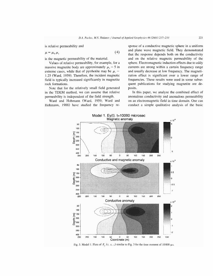
Fig. 6. Model l. Snap-shots of the vertical components of magnetic field Hz ( I, x, z )j31 in the case of a horizontal plate for the time moment of 100 p.s. The top panel corresponds to the case of a purely magnetic anomaly (P 2 = PI = 100 n m) with the relative magnetic permeability of the plate Il = 5. The bottom panel presents the results for the case of a purely conductive anomaly ( P2 = I n m, Il = 0,r r and the middle panel demonstrates the combined effect of magnetic and conductive anomalies ( P2 = 1 n m, Il r = 5).

- - ----

223 D.A. Parlor. M.S. Zhdanou/ Journal ofApplied Geophysics 46 (200 /) 2 /7-233

permeab ility and conductivity, /-L, 0' . The first term In order to conduct the quantit ative co mparative reflects the effect of magnetic charges caused by analysis of the anomalous conductiv ity and anoma­magnetic inhomogeneities . In the case of the piece­ lous perm eabil ity effects on TDEM response, we wise constant distribution of /-L" these charges are apply numerical modelin g techn ique. concentrated on the boundaries of the anomalous body. The seco nd term reflects the combined effects of both relative perme ability and conductivity. The

3. Numerical modeling of tim e domain responsesincreased perm eabi lity or increased conductivity for 3-D bodies with anomalous conductivity and within same volume results in the same effect of permeabilityincreasing the volume den sity of eddy currents within

an inhomogene ous domain . Therefore, we can distin­guish between the anomalous perm eabi lity and We consider the two typica l models presented in anomalous conductivity effects only because of the Fig. I . Model 1 (Fig, I, top panel) consists of a boundary effec t of the magnetic anoma ly. horizont al rect angular plate with lateral dimensions

Model 1. dHz(t)/dt. t=1000 microsec Magnetic anomaly

50

100

:[150

s: 200 Ci ~ 250

300

350

-200 -150 -100 -50 o 50 100 150 200 250

Conductive and magnetic anomaly

50 ..100 ... ( ((r1\r;J~')'

:[ 150 "="·-:.V s: 200

~ 250 o

300

350

400 -'-----.,.---,-----~--~"'-_,..'.:--.,._'-_,..--

-250 -200 -150 -100 -50 o 50 100 150 200 250

Conductive anomaly

50 l ~ ..-.- - - --_<, (~= _ .::. -----.._--'" l00 -V -..

<.:~ E 150 "'__.. - -_ . ,/' -.......- <>:;; 200 I -. - I g- 250 i o '

300 J I

350 1 400 -r-- ---,--- -....,-- - ---- - ----,- -,-----,- ­

250 200 150 100 50 0 50 100 150 200 250 Coordinate (m)

· 0.02

-0.03

0.03

0.02

0.01

o

A/(s'm )

Fig. 7. Model I. Plots of the vertical components of magneti c field liz ( r, x. : )j ot similar to Fig . 6 for the time moment of 1000 J.l. S.

224 D.A. Pacloc, M.S. Zhdanoc / Journal ofApplied Geophysics 46 1200 / ) 2 / 7-233

200 X 200 m, and a thickness of 40 m. loca ted at a P2 = 10 fl m. The transien t electromagnetic fie ld in depth of 100 m wi thin a homogeneou s, conduct ive the model was genera ted by a step pulse of electric half-space with a resistivi ty of PI = 100 fl m, and current in a rec tang ular loop of size 50 X 50 m, magnetic permeability of free space, fLo' Model 2 located on the ground above the center of the plate. (F ig. 1, bottom panel) consists of a vertical rectangu­ Numerical modeling was conducted using time do ­lar plate with lateral dimensio ns 40 X 200 m, and the mai n finite-difference code developed by Wan g and vertical size 200 m, located at a dep th of 100 m Hohmann (I 993). within the homogeneous, conductive half-space with Th e followi ng three cases are studied: resi stivity of PI = 100 fl m, and magnet ic perm e­abi lity of free space, fLo. We conducted a set of nume rica l experiments in which the relat ive perme­ I . the plate is charac terized by anomalous mag­ability fLr of the plate was equa l subsequently to I , 5 net ic permeability only (pure ly magnet ic and 10, and the resistivity of the plate was set to be anomaly); equal to the background resistivity P2 = 100 fl m, 2. the plate is characterized by anomalous conduc­or the plat e was a goo d conductor: P2 = I fl m, or tiv ity only (pure ly co nductive anoma ly); and

Model 1. dHz(t)/dt. t=10000 microsec Magnetic anomaly x 10..(,

2SO . 200 l SO . 100 ·50 a so 100 lSO 200 2SO

Conductive and magnetic anomaly

soJ ."-..."-... ( /:7 ; D\'\ j/~ 100

'E15O J ~ I -----• -----­l:r-- --~

a . 1

350 -2

~ . 1

so 100

:[ 150

..<: 200 C.(lJ 2SO o

300

3SO

400

3

2.5

2

1.5

2SO 200 150 100 50 a so 100 150 200 250

Conductive anomaly

SO ; - - ' - .i->: (;;;~7..~--~-:'~"

c ~100 ~ _ . _.. ~~\\ ~) ~E 150 " I .. ' - - -- - - - • _______ -.

i 200 i-----.-~.- '. 3

~ ::fi- -------.-- ----------- - ­.------ ­ 2.5 350 · _ - - - - - -- - - - - - __

L -------~ -----­4OO ! 'I t i ­

-2SO -200 .1SO -100 ·SO 0 so 100 ISO 200 2SO AI(s'm) Coordinate (m)

Fig. 8. Model I. Plots of the vertical components of magnetic field Hz (I . .r , : )/01 similar to Fig . 6 for the time moment of 10 000 u s.

225 D.A. Pavlov, M.S. Zhdanov / Journal ofApplied Geophysics 46 (2001) 217-233

3. the plate has both anomalous magnetic perme­ability and anomalous conductivity (combined magnetic and conductive anomaly).

Fig. 2 (top panel) presents the plots of (aH;)/(at) component measured in the center of the loop versus time for Modell. The solid line corresponds to magnetic field decay for the homogeneous half-space with a resistivity of 100 n m (background model). The line formed by crosses is the magnetic response for a purely conductive plate with a resistivity of 1 n m (conductive anomaly). An increase in the re­sponse occurs within the time interval from 2 X 10- 4

to 1 X 10- 2 s. The line formed by the stars is the magnetic response for a conductive plate with a resistivity of 10 n m (conductive anomaly only). One can see that the anomalous effect is very small in this case. The dotted line is the magnetic response for the case of a purely magnetic plate with J-Lr = 10 (magnetic anomaly). This line practically coincides with the solid curve, showing that the anomalous effect is very small in this case as well. Note that the product J-Lr (J" is the same for the case of the purely conductive anomaly with a resistivity of IOn m (the curve formed by stars), and for the purely magnetic anomaly with a relative magnetic perme­ability J-Lr = 10, and a background resistivity of 100 n m (the dotted line in Fig. 2, top panel). The only difference between these two cases is in the presence of the excess magnetic charges at the boundary of the plate. We can conclude that the contribution of these charges is negligibly small, because the corre­sponding curves practically coincide.

Fig. 2 (bottom panel) shows the results for a combined conductive and magnetic anomaly with different magnetic permeabilities for a plate with a resistivity of 1 n m. The solid line corresponds again to magnetic field decay for a homogeneous half-space. The line formed by crosses describes the effect due to eddy currents in a purely conductive anomaly. The dashed line presents the combined effect of anomalous magnetic permeability and anomalous conductivity for J-Lr = 5. We can observe an anomaly in the magnetic field decay behavior for a wider time interval than in the case of a purely conductive anomaly. Additional increase in relative magnetic permeability up to 10, leads to further increase of the anomalous effect on (aHz)/(at) de­

cay (shown by the dotted line in Fig. 2, bottom panel) and to shifting this anomaly toward the later time.

We have used numerical modeling to study the electromagnetic field propagation pattern within the model. Figs. 3-8 show the snap-shots of the horizon­tal component of electric field Ey (x, z. t ) and of the time denvative of the vertical component of magnetic field (aHz (x, Z, t)) I(at) in the vertical plane XZ crossing the horizontal plate in the middle along the axis X. The snap-shots were generated using a finite-difference code for the time moments 100, 1000, and 10000 p.s.

Model2. Conductiveor magneticanomaly 10' « -'-~~r-r-r--~~~~----r-c~-,-------~-~~,-,-~..,.--~----.,

magneticanomaly, !Ar=10

aN ~10--4

10-5

10-6

10-7

10'

10°

10-'

10-2

~

,.~ <.:::::> ~<~"

background conductiveanomaly ~=5

!1~=10

~10-S -, ~ ..

eN ..... ~10-4 .....

x. 10-5 ".

10-6

10-7

w--4 w~ w~

Time(s)

Fig. 9. Top panel: observed field aHz(t)/at versus time for Model 2 above the center of the anomaly. Bottom panel: observed field aHz(t)/at versus time for model 2 above the center of the anomaly for different magnetic permeabilities.

background conductiveanomaly

10-2

10°

:!2 10­S

10-4 10-3 10-2

Time(s)

Model2. Combinedconductiveand magneticanomaly

- -

226 D.A. Pavlov. M.S. Zhdanou / Journal ofApplied Geophysics 46 (200 1) 2 / 7-233

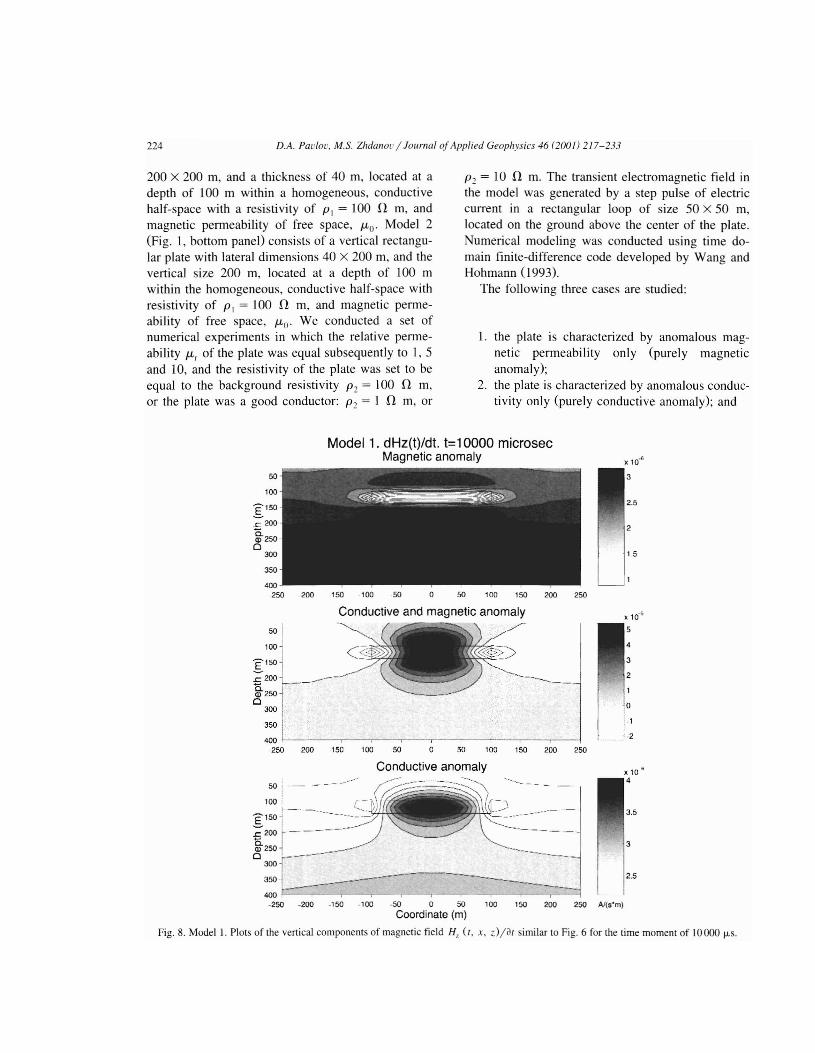
One can see three panels in each of Figs. 3-8. The top panel corresponds to the case of a purely magnetic anomaly (P 2 = PI = 100 n m) with the relative mag netic permeability of the body fLr = 5. The bottom panel present s the results for the case of a purely conductive anomaly ( P2 = I n m, fLr = l ), and the middle panel demonstrates the combined effec t of magnetic and conductive anomalies ( P2 = I n m, fL r = 5). In the ear ly time (up to 100 fLS), the behavior of the electromagnetic field is more or less similar for all three cases. It propagates downward and reaches the plate with the anomalous electro­

magnetic parameters (Figs. 3 and 6). At 1000 fL S, we already see significant differences in field behavior, espec ially between the models without (top panel) and with (middle and botto m panels) conductive anoma lies. In the case of a pure ly magnetic anomaly, we observe increase of the magnetic field and corre ­sponding increase of the electric fie ld in the anoma­lous part of the cro ss-section . However, this increase is smaller than in the presence of the conductive anomaly and is practically confined within the boundaries of the body , as one can see in Figs. 4 and 7.

Model 2. Ey(t). t=100 microsec Magnetic anomaly

50 {'_ -- --------­

' 00 .- -~ 1 50 ( - - - --­

~ 200 . '-. ---. - - - - - - ­

!~t~ --=:/ . -- --~.=-_= -~-=~-: :: ~: II'~.J

----: :;..-..::

-250 -200 - ' 50 -' 00 -50 0 50 100 150 200 250

Conductive and magnetic anomaly

50 r~~--=--=-..:: ~==---==---~----::. 100 V' ....-.. )" < -;<.'

~ ' 5O i I•.. ..j / / iJ­-~200 t'·~ - - - - - ..--:/(

~ 25O f------------ /::t----.----~ 400 . . . . · 250 · 200 -150 · 100 ·50 0 50 100 150 200 250

Conduct ive anomaly

,::r:---;=.:=--~~::~~-==~~--:.=~:--=-~,

I150 ~' ".-------- . //:/"­f: r - - ..../:Y)It 200 .~-...- --_ _ . ----/

~ 250 -~ - -.

300

350 ------.--- ­

400 I: , , i "p~ r I

o

-0 .02

004

0.06

0.05

o

· 0.05

o

1.0.05 - 250 -200 -150 .100 · 50 0 50 100 150 200 250 Vim

Coordinate (m)

Fig. 10. Model 2. Snap-shots of the horizontal components of electrical field E, ( r, x, z) in the case of a vert ical dike for the time moment of 100 J-L s. The top panel corresponds to the case of a purely magnetic anomaly (P1 = PI = 100 fl m) with the relative magnetic permeability of the dike fJ.- r = 5. The bottom panel present s the results for the case of a purely conductive anomaly ( P1 = I fl m, fJ.- , = I), and the midd le panel demonstrates the combined effect of magnetic and cond uctive anomalies ( P1 = I fl m, fJ.- , = 5).

-------

227 D.A. Pavlov, M.S. Zhdanou / Journal of Applied Geophysics 46 (2001) 217-233

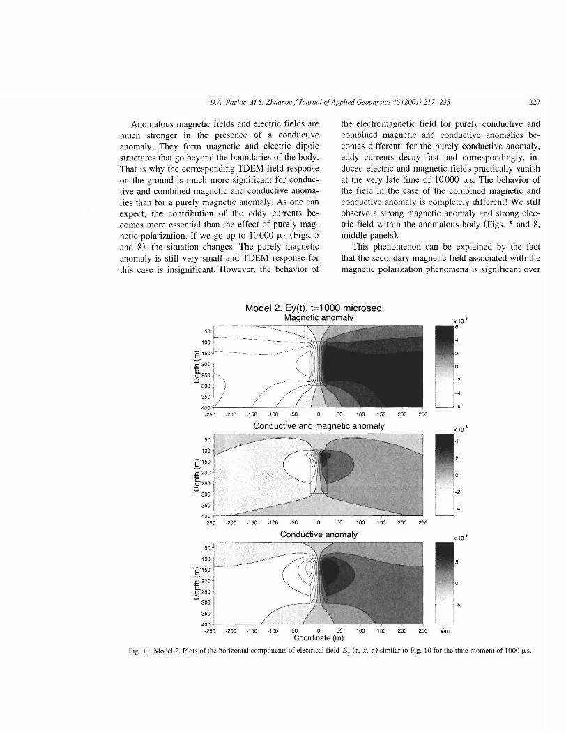
Anomalous magnetic fields and elec tric fields are much stronger in the presence of a conductive anomaly. They form magnetic and electric dipo le structures that go beyond the boundaries of the body. That is why the corresponding TDEM field response on the ground is much more significant for conduc­tive and combined magnetic and cond uctive anoma­lies than for a purely magnetic anomaly. As one can expect, the contribution of the eddy currents be­comes more essential than the effec t of purely mag­netic polarization. If we go up to 10000 u.s (Figs. 5 and 8), the situation changes. The purely magne tic anomaly is still very small and TDEM response for this case is insignificant. However, the behavior of

the electromagnetic field for purely conductive and combined magnetic and conductive anomalies be­comes different: for the purely conductive anomaly, eddy currents decay fast and correspondingly, in­duced electric and magnetic fields practically vanish at the very late time of 10 000 u.s, The behavior of the field in the case of the comb ined magnetic and conductive anomaly is completely different! We still observe a strong magnetic anomaly and strong elec­tric field within the anomalous body (Figs . 5 and 8, middle panels).

This phenomenon can be explained by the fact that the secondary magnetic field associated with the magnetic polarization phenomena is significant over

Model 2. Ey(t). t=1000 microsec Magnetic anomaly

so

2

o

'>. \ i-2

:.i 3S0 j /

'_ _ " 6400 -IL­

x 10' -~~_. . . Q --- .-..-:'---~

100 2

:[1S0

s: 200 o0.. Q) 2S0 o -2300

, 4

400 I -r -200 -l S0 .100 -so o so 100 150 200 250

3S0 .----~---I

·2S0 · 200 ·1S0 ·100 ·SO o 50 100 150 200 2S0

Conductive and magnetic anomaly

.2S0 ~ Conductive anomaly x 10 5

5

:[150

so

100

s: 200 o0.. Q) 250 c

300 ' -5

350 I~,400 I I ( \.- - -- ..-......-;

-2S0 -200 -1S0 -100 -so 0 50 100 150 200 250 Vim Coord inate (m)

Fig. II. Model 2. Plots of the horizontal components of electrical field E, (r , x , e) similar to Fig. 10 for the time moment of 1000 iLS.

--- - - - - - -

228 D.A. Pavlov. M.S. Zhdanoc / Journal ofApplied Geophysics 46 (200 / ) 2/ 7- 233

a much longer time period than eddy currents, be­cause it is connected with the magnetic field itself and not with its time derivative. Eddy currents, strong in the ear ly stages, generate a strong anom a­lous magnetic field, which is magnified in the mag­netized body due to magnetization phenomena. This effec t can be understood based on the induction Eq. (6) . The term ( ILl) IL, (J" (aE /a t)) in this equation, describing the eddy currents, amplifies significantly in the case of the combined magnetic and conductive anomaly, because both the relative permeability and conductivity increase in this case . With passing time, the eddy currents themselves attenuate quickly, but the genera ted induce d magnetic field stays much

longer. This effec t results in the shifting of the TDEM anoma lous response to the later times, and in its general increa se in the case of the combined magnetic and conductive anomalies .

Consider now the results of numerical modeling for Mode l 2 (Fig. I , bottom panel) . We conducted a set of numerical experiments in which the relative permeability IL, of the vertical dike was subse­quently equal to I , 5 and 10, and the resistivity of the dike was set to be equal to the background resistivity P: = 100 fl m, or the dike was a good conductor with P: = I fl m.

Note that the relative permeability value of 10 is extremely high and can be rarely observe d in actual

Model 2. Ey(t). t=10000 microsec Magnetic anomaly x 10 1\

-£ .cVU l I 10

1t 250 Cl f i·0 5300 i

350 '1

l , ,1 11 11

- ....-- _•.::fI) / \

,\f -: <' .::- LJ·l ' L / /-we

. ...... b ~ . .400 250 200 150 100 50 0 50 100 150 200 250

Conductive and magnetic anomaly x 10-8

50 J ~--~

I ! ! 111111 -/f, ~ ,.:"" - ,_ ·1 .2

100 1<

:[1 50 ] .J:: 200 ., ,

:"' .. g. 250 I

o 300 1

350 :

400 1 . 250 200 150 100 50 0 50 100 150 200 250

Conduct ive anomaly

o

I 1 0

-250 . 200 -150 .100 -50 0 50 100 150 200 250 Vim Coordinate (m)

Fig. 12. Mode l 2. Plots of the horizontal components of electrical field Ey ( t , x , z) similar to Fig. 10 for the time moment of 10000 J.l. S.

D.A. Pavlov. M.S. Zhdanou / Journal ofApplied Geophysics 46 (200n 217- 233 229

rock formations. Neverthele ss, we incl ude this value ability anomaly I-tr = 10. This line shows very litt le in our anal ysis to demonstrate that even in this anomalous effect in the TDEM response. The line extreme case, the pure ly magnetic anomaly will still form ed by crosses describes the effect due to the produce a little effect on TDEM data . edd y current in the pure ly conductive dike. In this

Fig . 9 (top panel) presents the plots of the case, it is almost as small as the effect of the purely (aH

7) I (af ) component measured in the center of the magnetic anomaly.

loop versus time for Model 2. The solid line corre­ Fig . 9 (bottom panel) shows the response for the sponds to magnetic field decay for a homogeneous purely conductive anomaly and for the combined half-space with a resistivi ty of 100 n m (back­ conductive and magnetic anomalies. The resistivity ground model). The dotted line is the magnetic of the dike is equal the P2 = 1 n m. The so lid line response for a case with the purel y magnetic perme- corre sponds again to magnetic field decay for a

Model 2. dHz(t)/dt. t=100 microsec Magnetic anomaly

1 :: ~ (" ~~~c:~»/) /)~ :::~<" , .~",- ,·_·":"~~'::'~~~~=~1~:~~~~~-~~'~~'~~:=~-" " //~._ . a. ! Q) 250 c o

300 !i

350 ~

1400 .+-- ---,-- - - --.-- --,--,--- .,---,---,-----r----,

250 200 · 150 ·100 50 o 50 100 150 200 250

Conductive and magnetic anomaly

50 / / (~- ~-.:==~ -~) ) 1

100 .. \ -, ~.. //... ~ - v , '\..-• • _ _ .. / ../

E 150 ­ \ ..'- ',' -.... " .

-" ' - ' " .c 200 : \:1. _ - __." _, J

g. 250 ­0

300 ­

350 ,

400 ·250 . 200 .150 ·100 · 50 50 100 150 200 250

Conductive anomaly

50 ~ ( ( C/"= ''''') ~'\ ')i

100 ' \ -, -\~:-- ..) E1 50

s: 200 15. Q) 250 o

300

350

400

"\..-.~ ..- ......_- , ..~~I l .., - _..... > /

<,<,<,.... · .. ....····-----0 -----··......···.. ..--/ °250 200 150 100 50 50 100 150 200 250

Coordinate (m)

0.5

0.4

0.3

0.2

1°·1

O.B

0.6

i10.4

1 ! 0.2

N(s' m)

Fig. 13. Model 2. Snap- shots of the vertical components of magnetic field Hz (I . .r, ~ )/a l in the case of a vertical dike for the time moment of 100 u.s. The top panel corresponds to the case of a purely magnetic anomaly ( P2 = PI = lOa n m) with the relative magnetic permeabil ity of the dike /1-, = 5. The bottom panel presents the results for the case of a purely conductive anomaly ( P2 = I .n m, /1-, = n and the middle panel demon strates the combined effect of magnetic and conductive anomalies ( P2 = I .n m. /1-, = 5).

230 D.A. Parlo r, M.S. Zhdanoc / Journal ofApplied Geophysics 46 (lOO/) 217- 233

homogeneous conductive half-space (bac kgro und model) . The line formed by crosses shows again the effect of the purely conductive anomaly. The dashed line present s the combined effect of anomalous mag­netic permeability and anomalous conductivity for J.L = 5. We can observe an anomaly in the magnet ic r field decay behavior for a rather wide time interval. If we increase the relat ive permeabilit y of the plate up to 10, the anomalous effect grows significa ntly and extends till the later times (shown by the dotted line in Fig. 9, bottom panel).

Similar to Modell , we have studied numerically the electromagnetic field propagation pattern within Model 2. The snap-shots of the horizont al compo­

....--..J

200 150 100 50 0 50 100 150 200 250

50 f

Conductive and magnetic anomaly , 15

/ --- - --­50

100

:[150 10

s: 200

5g. 250 Cl

300 o 350

· 5 400

· 250 ·200 ·150 ·100 ·50 0 50 100 150 200 250

nent of electric field E, (x , Z, r), and of the time derivative of the vertical component of magnetic field csn, (x, Z, t ))I (ar) in the vertical plane XZ crossing the vertical dike plate in the middle along the axis X, are show n in Figs. 10- 15. We have selected the same time moments as for Model I : 100, 1000, and 10 000 p.s,

The top panels in Figs . 10-15 correspond to the case of a purely magnetic anomaly ( pz = PI = 100 n m) with the relative magnetic permeability of the body J.Lr = 5. The bottom panels present the results for the case of a purel y condu ctive anomaly ( pz = I n m, J.Lr = I), and the middl e panels demonstrate the combined effect of magnet ic and conductive anoma-

X 10"

1.6

1.4

1.2

50

100

:[1 50

s: 200

c3a.250

300

350

400 t , ..

Conductive anomaly X 10-3

5

4.5

4

3.5

3 . .,,,( 2.5

2\ "'-, //

.~~-- 1.5 .......

· 250 200 · 150 .100·50 0 50 100 150 200 250 A/(s'm)

Coordinate (m) Fig. 14. Model 2. Plots of the vertica l compone nts of mag netic field H, (t, .r, z )j at similar to Fig. 13 for the time moment of 1000 IJ.S.

I D.A. Pavlov, M,S. Zhdanou / Journal of Applied Geophysics 46 (200 J) 217-233 23 1

I

50 L .. - __----------. .--..........-- -_ ..J

350

400 ·250 -200 -150 -100 -50 50 100 150 200 250

Conductive and magnetic anomaly

-1:: ~ -------....... (~_) -.......--------; ~1 50 " (_. / ( v,''--''\ ') "-. .....\ ; .§. , ----. ......... ( \ ~/B~\ \ ! ) ' "........-- ---1 ~ 200- "-, \.. ' \:1 011:1 / ....»<

8 '~ i-- -------_~~~~---------'J 300 1 .,..-,---_-r--. -- _ 350 r - -- ­

400 ' . 250 .200 .150 .100 50 o 50 100 150 200 250

Conductive anomaly 50 .____ _ . ­

100 " -- -----­

I:F---- -==: - ~~: : --==-::= :<'i '~ - -. .'

- I 350

400

X io"

4

3.5

3

25

2

x 10 8

3

2.9

28

2.7

2.6

25

2

'1 .42.3

-250 · 200 .150 -100 ·5 0 0 50 100 150 200 250 A/(S'm)

Coordinate (m)

Fig. 15. Model 2. Plots of the vertical components of magnetic field H, ( t . .v, : )/~ t similar to Fig. 13 for the time moment of 10 000 J.l. S.

lies ( P2 = I n m, JL = 5). We can see again that inr

the early time (up to 100 u s) the behavior of the electromagnetic field is similar for all three cases. It propa gates downw ard and reaches the top of the dike with the anomalous electromagnetic parameters (Figs . 10 and 13), At 1000 /-LS, the differences between these three models of different electromagnetic anomalies become significant, especially for the magnetic field components, In the case of a purely magnetic anomaly, we observe two induced mag­netic dipoles in the top and in the bottom of the dike with the positive anomaly directed outward of the dike (top panel in Fig. 14). In the case of a purely conductive anomaly, the maximum of the secondary

magnetic field is concentrated inside the dike (bot­tom panel in Fig. 14). This differe nce is related to the fact that eddy currents tend to reduce the changes in the incident magnet ic field B, while the magnetic permeability anomaly caused by paramagnetic mate­rial in the dike tends to increase the incident field . We see the combination of these two effects in the middle panel, which corresponds to the combined effec t of the conductivity and magnetic permeability anomalies.

The important difference between the modeling results for the horizontal plate and for the vertica l dike is that in the last case, the effect of the eddy currents is small and comparable with the effec t of

232 D.A. Pavlov, M.S. Zhdanov / Journal ofApplied Geophysics 46 (2001) 217-233

the purely magnetic anomaly. It can be explained by the fact that the horizontal transmitter loop generates the horizontal "smoke rings" of the current in the background media, which cannot induce significant eddy currents in the relatively thin vertical dike. Therefore, in the case of the dike, and considering the special geometry of the TDEM survey, the TDEM responses in the ground observations for both the purely magnetic and purely conductive anomalies are relatively small. We observe the same picture for the later time of up to 10 000 f-LS (Figs. 12 and 15). For purely magnetic anomalies, we still have a small effect which slowly attenuates with time, for purely conductive anomaly eddy currents decay fast and correspondingly induced electric and magnetic fields also disappear at the very late time of 10000 I-LS. However, the behavior of the field in the case of combined magnetic and conductive anomalies hap­pens to be very different. We continue to observe significant electric and magnetic anomalies even for a very late time (Figs. 12 and 15, middle panels), because the secondary magnetic field induced by the eddy currents in the earlier time and magnified by the magnetic polarization phenomena continues to be present even for late time observations. This effect is observed on the TDEM decay curves in shifting the anomalous response to the later times.

4. Conclusion

The results of the numerical study have demon­strated that anomalous magnetic permeability of an ore body could result in a significant anomalous effect on the TDEM data. This effect is magnified in the presence of combined conductive and magnetic anomalies. Anomalous magnetic permeability pro­longs the anomalous TDEM response to the later times, and increases it overall in comparison with the purely anomalous conductivity effect.

Formal interpretation of TDEM data over simulta­neously conductive and magnetized geological struc­tures could produce erroneous results. Therefore, the magnetization effects should be taken into account in developing the methods of TDEM data interpretation in mineral exploration.

We will present a new method for simultaneous inversion of TDEM data for anomalous conductivity and magnetic permeability in the accompanying pa­per (Zhdanov and Pavlov, 2001).

Acknowledgements

The authors acknowledge the support of the Uni­versity of Utah Consortium for Electromagnetic Modeling and Inversion (CEMI), which includes 3JTECH, Advanced Power Technologies, Agip, Baker Atlas Logging Services, BHP Minerals, EXXON Production Research, INCO Exploration, Japan National Oil Corporation, MINDECO, MO­BIL Exploration and Production Technical Center, Naval Research Laboratory, Newmont Gold, Rio Tinto, Shell International Exploration and Produc­tion, Schlumberger-Doll Research, Unocal Geother­mal, and Zonge Engineering.

We are thankful to Mr. J. Inman from Kennecott Exploration (Rio Tinto) for fruitful discussions and comments.

We are grateful to the reviewers, Drs. P. Weidelt and Z. Xiong, for their useful comments and recom­mendations.

References

Fraser, D., 1981. Magnetite mapping with a multicoil airborne electromagnetic system. Geophysics 46, 1579-1593.

Kaufman, A.A., Karinsky, A.D., Wightman, W.E., 1996. Influ­ence of inductive effect on measurements of resistivity through casing. Geophysics 61, 32-34.

Olhoeft, G.R., Strangway, D.W., 1974. Magnetic relaxation and electromagnetic response parameter. Geophysics 39, 302-311.

Strack, K.M., Fanini, 0., Maurer, H.-M., Singer, B.S., Tabarovsky, L.A., 1996. Measurements of formation resistivity through a metal casing. GeoArabia-Middle East Petroleum Geosciences 1 (1), 198-210, March GEO'96 Abstracts.

Wang, T., Hohmann, G.W., 1993. A finite-difference time domain solution for three-dimensional electromagnetic modeling. Geo­physics 58, 797-809.

Ward, S.H., 1959. Unique determination of conductivity, suscepti­bility, size, and depth in multifrequency electromagnetic ex­ploration. Geophysics 24, 531-546.

Ward, S.H., Hohmann, G.W., 1988. Electromagnetic Theory for Geophysical Applications: Electromagnetic Methods In Ap­

233 D.A. Pavlov, M.S. Zhdanov / Journal ofApplied Geophysics 46 (2001) 217-233

plied Geophysics, 1, Theory. Society of Exploration Geophys., Zhdanov, M.S., Pavlov, D.A., 2001. Analysis and interpretation of Tulsa, OK, pp. 131-308. anomalous conductivity and magnetic permeability effects in

Zhang, Z., Oldenburg, D.W., 1999. Simultaneous reconstruction time domain electromagnetic data. Part II: Su-inversion. Jour­of 1-D susceptibility and conductivity from electromagnetic nal of Applied Geophysics 46, 235-248. data. Geophysics 58, 33-47.