Analysis and Design of Algorithms. According to math historians the true origin of the word...
86
Analysis and Design of Algorithms
-
Upload
augusta-farmer -
Category
Documents
-
view
214 -
download
0
Transcript of Analysis and Design of Algorithms. According to math historians the true origin of the word...

Analysis and Design of Algorithms

According to math historians the true origin of the word algorism: comes from a famous Persian author named ál-Khâwrázmî.

Khâwrázmî (780-850 A.D.)
Statue of Khâwrázmî in front of the Faculty of Mathematics,Amirkabir University of Technology, Tehran, Iran.
A stamp issued September 6, 1983 in the Soviet Union, commemorating Khâwrázmî's 1200th birthday.
A page from his book.
Courtesy of Wikipedia

Computational Landscape
Design Methods:
Iteration & Recursion pre/post condition, loop invariant Incremental Divide-&-Conquer Prune-&-Search Greedy Dynamic programming Randomization Reduction …
Analysis Methods:
Mathematical Induction pre/post condition, loop invariant Asymptotic Notation Summation Recurrence Relation Lower and Upper Bounds Adversarial argument Decision tree Recursion tree Reduction …
Data Structures:
List, array, stack, queue Hash table Dictionary Priority Queue Disjoint Set Union Graph …
Computational Models:
Random Access Machine (RAM) Turing Machine Parallel Computation Distributed Computation Quantum Computation …

Algorithm
• An algorithm is a sequence of unambiguous instructions for solving a problem, i.e., for obtaining a required output for any legitimate input in a finite amount of time.
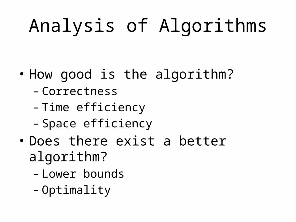
Analysis of Algorithms
• How good is the algorithm?– Correctness– Time efficiency– Space efficiency
• Does there exist a better algorithm?– Lower bounds– Optimality

Example
Time Complexity Execution time
n 1 sec
n log n 20 sec
n2 12 days
2n 40 quadrillion (1015) years
Let’s assume: Computer speed = 106 IPS, Input: a data base of size n = 106
Time complexity shows dependence of algorithm’s running time on input size.

Machine Model Algorithm Analysis:
should reveal intrinsic properties of the algorithm itself.
should not depend on any computing platform, programming
language, compiler, computer speed, etc.
Elementary steps:
arithmetic: + – logic: and or not
comparison: assigning a value to a scalar variable: ….
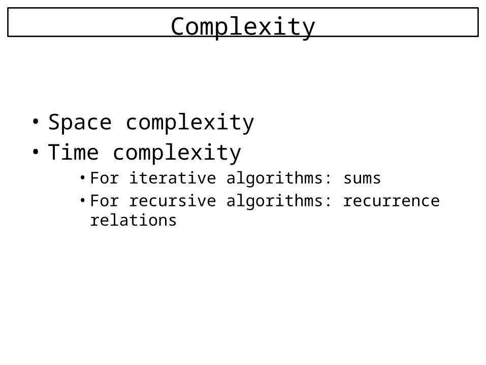
• Space complexity• Time complexity
• For iterative algorithms: sums• For recursive algorithms: recurrence relations
Complexity
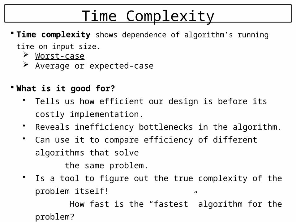
Time Complexity Time complexity shows dependence of algorithm’s running time on input size.
Worst-case Average or expected-case
What is it good for?
• Tells us how efficient our design is before its costly implementation.
• Reveals inefficiency bottlenecks in the algorithm.
• Can use it to compare efficiency of different algorithms that solve
the same problem.
• Is a tool to figure out the true complexity of the problem itself!
How fast is the “fastest” algorithm for the problem?
• Helps us classify problems by their time complexity.

T(n) = Q( f(n) )
T(n) = 23 n3 + 5 n2 log n + 7 n log2 n + 4 log n + 6.
drop lower order termsdrop constant multiplicative factor
T(n) = Q(n3)
Why do we want to do this?1. Asymptotically (at very large values of n) the leading term largely
determines function behaviour.2. With a new computer technology (say, 10 times faster) the leading
coefficient will change (be divided by 10). So, that coefficient is technology dependent any way!
3. This simplification is still capable of distinguishing between important but distinct complexity classes, e.g., linear vs. quadratic, or polynomial vs exponential.

Asymptotic Notations: Q O W o w
Theta f(n) = Q(g(n)) f(n) ≈c g(n)
Big Oh f(n) = O(g(n)) f(n) ≤c g(n)
Big Omega f(n) = Ω(g(n)) f(n) ≥ c g(n)
Little Oh f(n) = o(g(n)) f(n) c g(n)
Little Omega f(n) = ω(g(n)) f(n) c g(n)
Rough, intuitive meaning worth remembering:

limn→∞ f(n)/g(n)
0 order of growth of f(n) < order of growth of g(n)f(n) o(g(n)), f(n) O(g(n))
c>0 order of growth of f(n) = order of growth of g(n)f(n) (g(n)), f(n) O(g(n)), f(n) (g(n))
∞ order of growth of f(n) > order of growth of g(n)
f(n) (g(n)), f(n) (g(n))
=
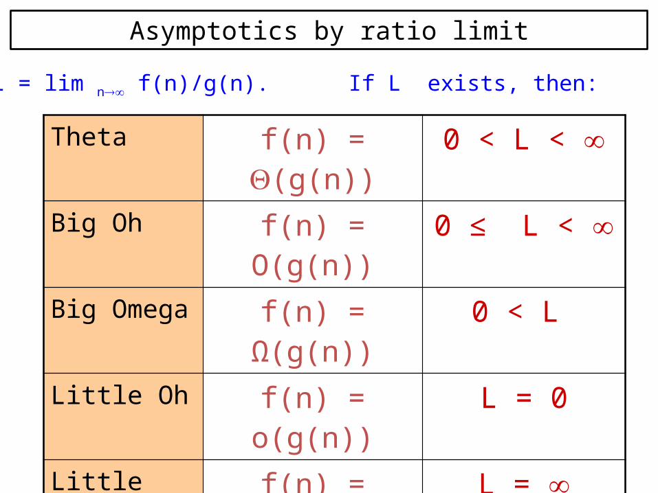
Asymptotics by ratio limit
Theta f(n) = Q(g(n)) 0 < L <
Big Oh f(n) = O(g(n)) 0 ≤ L <
Big Omega f(n) = Ω(g(n)) 0 < L
Little Oh f(n) = o(g(n)) L = 0
Little Omega f(n) = ω(g(n)) L =
L = lim n f(n)/g(n). If L exists, then:

Examples:• logb n vs. logc n
logbn = logbc logcn limn→∞( logbn / logcn) = limn→∞ (logbc) = logbc
logbn (logcn)

L’Hôpital’s rule
If limn→∞ t(n) = limn→∞ g(n) = ∞
The derivatives f´, g´ exist,
Then
t(n)g(n)
limn→∞
= t ´(n)g ´(n)
limn→∞
• Example: log2n vs. n

Theta : Asymptotic Tight Bound
f(n) = Q(g(n)) g(n)
c1g(n)
c2g(n) f(n)
n0 n
c1, c2, n0 >0 : n n0 , c1g(n) f(n) c2g(n).
+
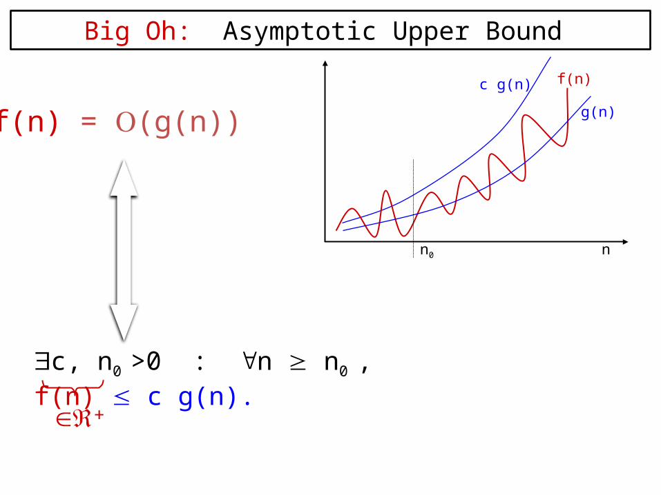
Big Oh: Asymptotic Upper Bound
f(n) = O(g(n))
c g(n) f(n)
n0 n
c, n0 >0 : n n0 , f(n) c g(n).
g(n)
+

Big Omega : Asymptotic Lower Bound
f(n) = W(g(n)) g(n)
c g(n)
f(n)
n0 n
c, n0 >0 : n n0 , cg(n) f(n).
+

Little oh : Non-tight Asymptotic Upper Bound
f(n) = o(g(n))c g(n)
f(n)
n0 n
c >0, n0 >0 : n n0 , f(n) < c g(n) .
No matter how small +

Little omega : Non-tight Asymptotic Lower Bound
f(n) = w(g(n))
c g(n)
f(n)
n0 n
c >0, n0 >0 : n n0 , f(n) > c g(n) .
No matter how large +
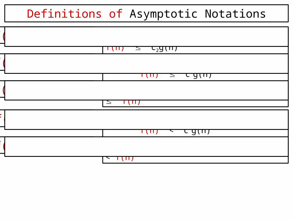
Definitions of Asymptotic Notations
f(n) = Q(g(n)) c1,c2>0, n0>0: n n0 , c1g(n) f(n) c2g(n)
f(n) = O(g(n)) c>0, n0>0: n n0 , f(n) c g(n)
f(n) = W(g(n)) c>0, n0 >0: n n0 , c g(n) f(n)
f(n) = o(g(n)) c >0, n0>0: n n0 , f(n) < c g(n)
f(n) = w(g(n)) c >0, n0>0: n n0 , c g(n) < f(n)


Ordering Functions
Functions
Constant
Logarithm
ic
Poly L
ogarithmic
Polynom
ial
Exponential
(log n)5 n5 25n5 log n5
<< << << << <<
<< << << << <<
Factorial
n!

Classifying Functions
Polynomial
Linear
Quadratic
Cubic
?
5n25n 5n3 5n4

Example Problem: Sorting
Some sorting algorithms and their worst-case time complexities:
Quick-Sort: Q(n2) Insertion-Sort: Q(n2)Selection-Sort: Q(n2)Merge-Sort: Q(n log n)Heap-Sort: Q(n log n)there are infinitely many sorting algorithms!
So, Merge-Sort and Heap-Sort are worst-case optimal, and
SORTING complexity is Q(n log n).

Theoretical analysis of time efficiency
Time efficiency is analyzed by determining the number of repetitions of the basic operation as a function of input size
Basic operation: the operation that contributes most towards the running time of the algorithm.
T(n) ≈ copC(n)running time execution time
for basic operation
Number of times basic operation is executed
input size

Problem Input size measure Basic operation
Search for key in list of n items
Number of items in list n Key comparison
Multiply two matrices of floating point numbers
Dimensions of matricesFloating point multiplication
Compute an nFloating point multiplication
Graph problem #vertices and/or edgesVisiting a vertex or traversing an edge
Input size and basic operation examples

Theoretical analysis of time efficiency
Time efficiency is analyzed by determining the number of repetitions of the basic operation as a function of input size

Best-case, average-case, worst-case
• Worst case: W(n) – maximum over inputs of size n
• Best case: B(n) – minimum over inputs of size n
• Average case: A(n) – “average” over inputs of size n– NOT the average of worst and best case– Under some assumption about the probability distribution of
all possible inputs of size n, calculate the weighted sum of expected C(n) (numbers of basic operation repetitions) over all possible inputs of size n.

32
Time efficiency of nonrecursive algorithms
Steps in mathematical analysis of nonrecursive algorithms: • Decide on parameter n indicating input’s size• Identify algorithm’s basic operation• Determine worst, average, & best case for inputs of size n• Set up summation for C(n) reflecting algorithm’s loop
structure• Simplify summation using standard formulas

Series
Proof by Gauss when 9 years old (!):2
)1(
1
NNiS
N
i
)1(2
123...)2()1(
)1()2(...321
NNS
NNNS
NNNS

General rules for sums
i
ii
kki
ii
kn
kmii
n
miki
ii
ii
ii
iii
ii
n
mi
n
mi
xaxxa
aa
acca
baba
mnccc
)(
)1(1

Some Mathematical Facts
• Some mathematical equalities are:
22
)1(*...21
2
1
nnnni
n
i
36
)12(*)1(*...41
3
1
22 nnnnni
n
i
122...21021
0
1
n
i
nni
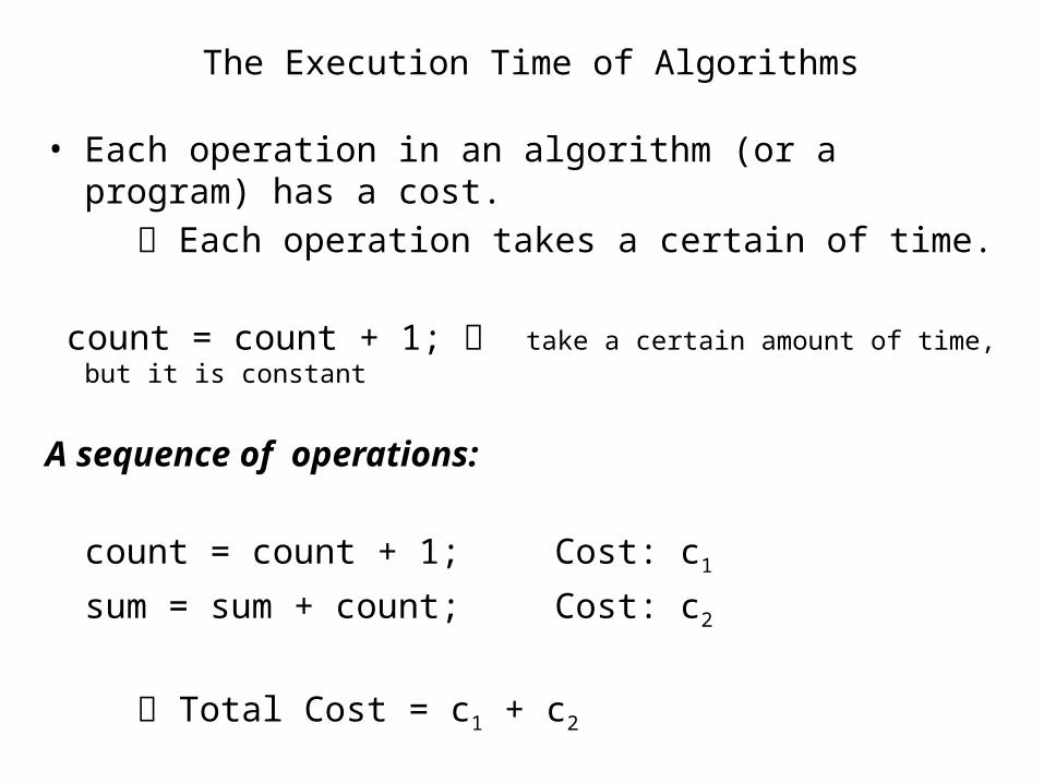
The Execution Time of Algorithms
• Each operation in an algorithm (or a program) has a cost. Each operation takes a certain of time.
count = count + 1; take a certain amount of time, but it is constant
A sequence of operations:
count = count + 1; Cost: c1
sum = sum + count; Cost: c2
Total Cost = c1 + c2
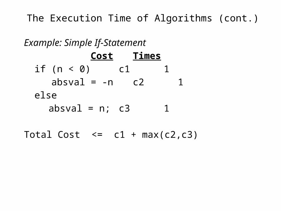
The Execution Time of Algorithms (cont.)
Example: Simple If-StatementCost Times
if (n < 0) c1 1 absval = -n c2 1else
absval = n; c3 1
Total Cost <= c1 + max(c2,c3)

The Execution Time of Algorithms (cont.)Example: Simple Loop
Cost Timesi = 1; c1 1sum = 0; c2 1while (i <= n) { c3 n+1
i = i + 1; c4 nsum = sum + i; c5 n
}
Total Cost = c1 + c2 + (n+1)*c3 + n*c4 + n*c5 The time required for this algorithm is proportional to n

The Execution Time of Algorithms (cont.)Example: Nested Loop
Cost Timesi=1; c1 1sum = 0; c2 1while (i <= n) { c3 n+1
j=1; c4 nwhile (j <= n) { c5 n*(n+1) sum = sum + i; c6 n*n j = j + 1; c7 n*n
} i = i +1; c8 n}
Total Cost = c1 + c2 + (n+1)*c3 + n*c4 + n*(n+1)*c5+n*n*c6+n*n*c7+n*c8 The time required for this algorithm is proportional to n2

Growth-Rate Functions – Example1Cost Times
i = 1; c1 1sum = 0; c2 1while (i <= n) { c3 n+1
i = i + 1; c4 nsum = sum + i; c5 n
}
T(n) = c1 + c2 + (n+1)*c3 + n*c4 + n*c5 = (c3+c4+c5)*n + (c1+c2+c3)= a*n + b
So, the growth-rate function for this algorithm is O(n)

Growth-Rate Functions – Example2Cost Times
i=1; c1 1sum = 0; c2 1while (i <= n) { c3 n+1
j=1; c4 nwhile (j <= n) { c5 n*(n+1) sum = sum + i; c6 n*n j = j + 1; c7 n*n
} i = i +1; c8 n}
T(n) = c1 + c2 + (n+1)*c3 + n*c4 + n*(n+1)*c5+n*n*c6+n*n*c7+n*c8= (c5+c6+c7)*n2 + (c3+c4+c5+c8)*n + (c1+c2+c3)= a*n2 + b*n + c
So, the growth-rate function for this algorithm is O(n2)
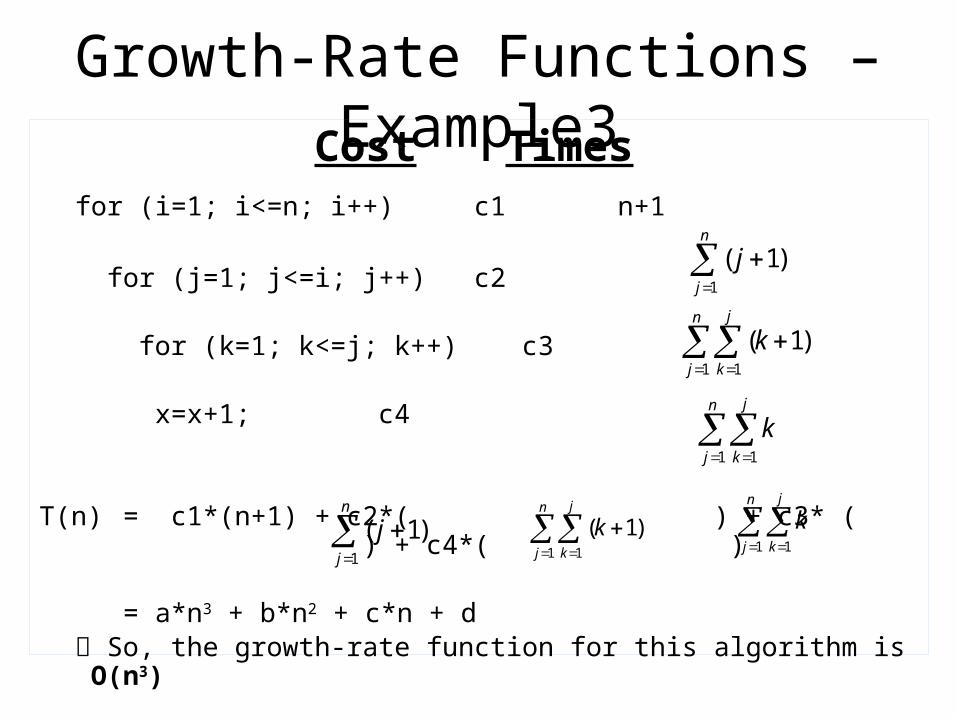
Growth-Rate Functions – Example3Cost Times
for (i=1; i<=n; i++) c1 n+1
for (j=1; j<=i; j++) c2
for (k=1; k<=j; k++) c3
x=x+1; c4
T(n) = c1*(n+1) + c2*( ) + c3* ( ) + c4*( )
= a*n3 + b*n2 + c*n + d So, the growth-rate function for this algorithm is O(n3)
n
j
j1
)1(
n
j
j
k
k1 1
)1(
n
j
j
k
k1 1
n
j
j1
)1(
n
j
j
k
k1 1
)1(
n
j
j
k
k1 1

Sequential Searchint sequentialSearch(const int a[], int item, int n){
for (int i = 0; i < n && a[i]!= item; i++);if (i == n)
return –1;return i;
}Unsuccessful Search: O(n)
Successful Search:Best-Case: item is in the first location of the array O(1)Worst-Case: item is in the last location of the array O(n)Average-Case: The number of key comparisons 1, 2, ..., n
O(n)n
nn
n
in
i 2/)( 21

Insertion Sort an incremental algorithm
2 4 5 7 11 15
2 4 5 7 11 15
2 11 5 7 4 15
2 5 11 7 4 15
2 5 11 7 4 15
2 5 11 7 4 15

Insertion Sort: Time Complexity
Algorithm InsertionSort(A[1..n]) for i 2 .. n do LI: A[1..i –1] is sorted, A[i..n] is untouched.
§ insert A[i] into sorted prefix A[1..i–1] by right-cyclic-shift: 2. key A[i]3. j i –14. while j > 0 and A[j] > key do5. A[j+1] A[j]6. j j –17. end-while8. A[j+1] key9. end-forend
.n1i 22
)1n(nn
2i
n
i
in2 .sorted) (reverseiterations it :case-Worst i
.n
nn2
2
n
iitn
2
n
iit
)n(T
2
11
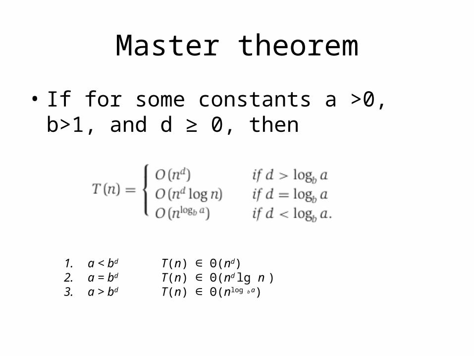
Master theorem
• If for some constants a >0, b>1, and d ≥ 0, then
1. a < bd T(n) ∈ Θ(nd) 2. a = bd T(n) ∈ Θ(nd lg n ) 3. a > bd T(n) ∈ Θ(nlog b a)

The divide-and-conquer Design Paradigm
• Divide the problem into subproblems.• Conquer the subproblems by solving them
recursively.• Combine subproblem solutions.
• Many algorithms use this paradigm.

Divide-and-conquer Technique
subproblem 2 of size n/2
subproblem 1 of size n/2
a solution to subproblem 1
a solution tothe original problem
a solution to subproblem 2
a problem of size n

49
Divide and Conquer Examples
• Sorting: mergesort and quicksort• Matrix multiplication-Strassen’s algorithm• Binary search• Powering a Number• Closest pair problem• ….etc.

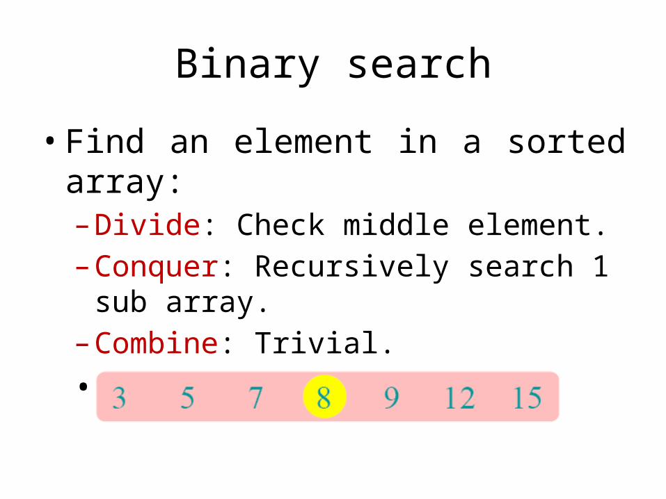
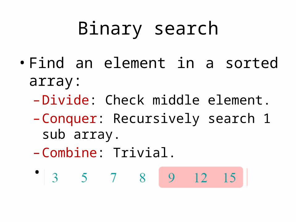
Binary search
• Find an element in a sorted array:– Divide: Check middle element.– Conquer: Recursively search 1 sub array.– Combine: Trivial.• Example: Find 9 3 5 7 8 9 12 15

Binary search
• Find an element in a sorted array:– Divide: Check middle element.– Conquer: Recursively search 1 sub array.– Combine: Trivial.• Example: Find 9
Binary search
• Find an element in a sorted array:– Divide: Check middle element.– Conquer: Recursively search 1 sub array.– Combine: Trivial.• Example: Find 9
Binary search
• Find an element in a sorted array:– Divide: Check middle element.– Conquer: Recursively search 1 sub array.– Combine: Trivial.• Example: Find 9

Binary search
• Find an element in a sorted array:– Divide: Check middle element.– Conquer: Recursively search 1 sub array.– Combine: Trivial.• Example: Find 9

Binary search
• Find an element in a sorted array:– Divide: Check middle element.– Conquer: Recursively search 1 sub array.– Combine: Trivial.• Example: Find 9

Binary search
• Find an element in a sorted array:– Divide: Check middle element.– Conquer: Recursively search 1 sub array.– Combine: Trivial.• Example: Find 9

Binary Searchint binarySearch(int a[], int size, int x) { int low =0; int high = size –1; int mid; // mid will be the index of // target when it’s found. while (low <= high) { mid = (low + high)/2;
if (a[mid] < x) low = mid + 1;
else if (a[mid] > x) high = mid – 1;
else return mid;
} return –1;}
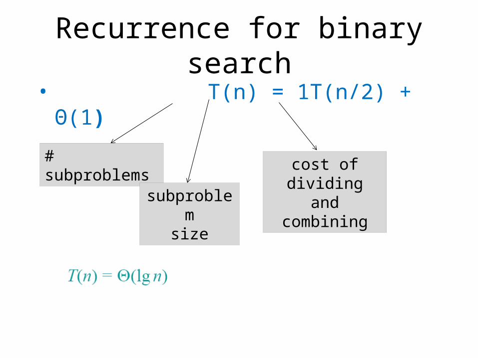
Recurrence for binary search• T(n) = 1T(n/2) + Θ(1)
# subproblems
subproblemsize
cost of dividing and combining

How much better is O(log2n)?
n O(log2n)16 464 6256 81024 (1KB) 1016,384 14131,072 17262,144 18524,288 191,048,576 (1MB) 201,073,741,824 (1GB) 30

Powering a Number
• Problem: Compute an, where n N.∈• Naive algorithm:
– Multiply n copies of X: X ·X ·X ··· X ·X ·X. – Complexity ? Θ(n)
• The Spot Creativity:– Is this the only and the best algorithm?– Any Suggestions on using divide-and-conquer
strategy?

Powering a Number
• Starting with X, repeatedly multiply the result by itself. We get:
• X, X2, X4, X8, X16, X32, …• Suppose we want to compute X13.• 13 = 8 + 4 + 1. So, X13 = X8 ·X4 ·X.

• Divide-and-conquer:
• Complexity:T(n) = T(n/2) + Θ(1)
T(n) = Θ(lgn)
Powering a Number
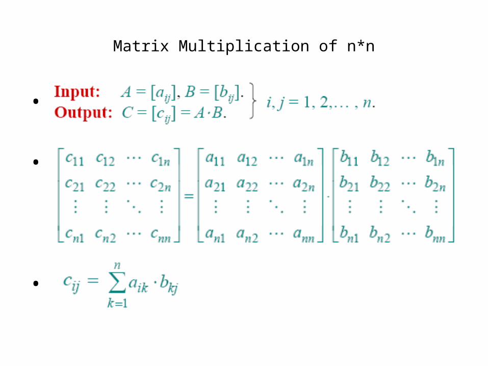
Matrix Multiplication of n*n
•
•
•

Code for Matrix Multiplication
•
for i=1 to nfor j=1 to n
cij=0
for k=1 to ncij=cij + aik*bkj
• Running Time= ?
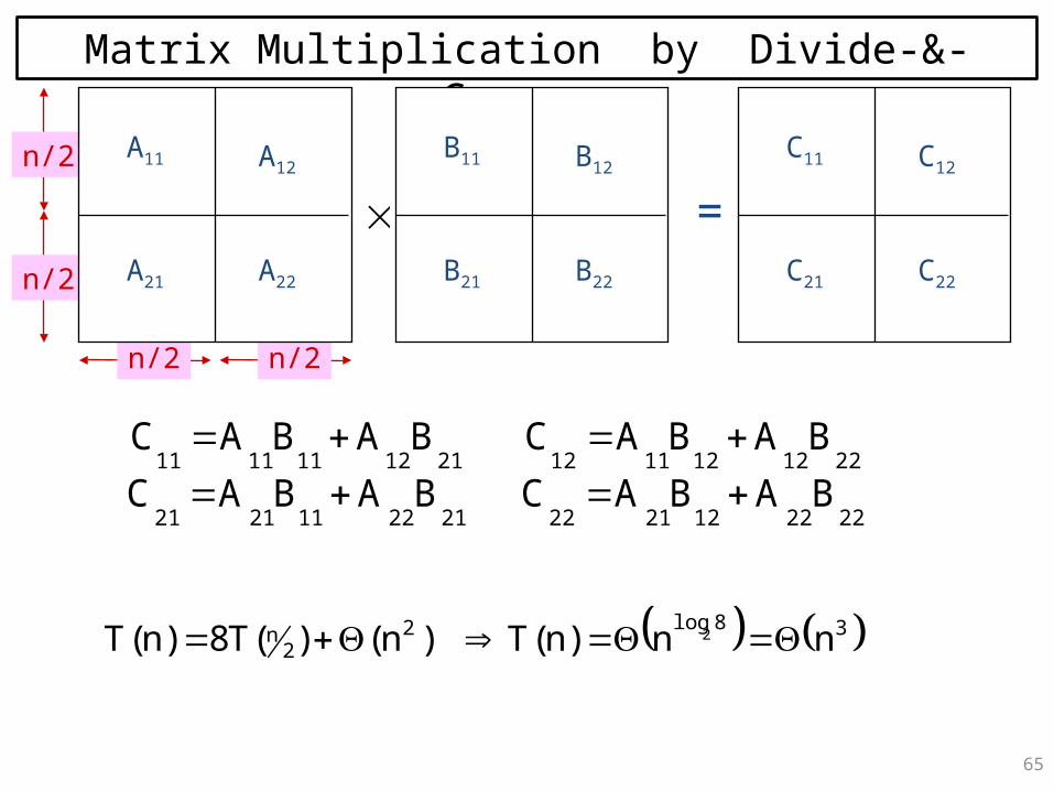
Matrix Multiplication by Divide-&-Conquer
22221221222122112121
22121211122112111111
BABACBABAC
BABACBABAC
n/2
n/2
n/2
n/2
=
A11 A12
A21 A22
B11 B12
B21 B22
C11 C12
C21 C22
38log22
n nn)n(T)n()(T8)n(T 2
65

Strassen’s Idea• How Strassen came up with his magic idea?
– We should try get rid of as more multiplications as possible. We could do a hundred additions instead.
– We can reduce the numbers of subproblems in T(n)=8 * T(n/2) + Θ(n2)– He must be very clever.

Strassen’s Idea
• Multiply 2*2 matrices with only 7 recursive multiplications.
• Notes: plus of matrices is commutative , but multiplication is not.

Strassen’s Algorithm
1.Divide: Partition A and B into (n/2)*(n/2) submatrices. And form terms to be multiplied using + and –.
2.Conquer: Perform 7 multiplications (P1 to P7) of (n/2)×(n/2) submatrices recursively.
3.Combine:Form C (r,s,t,u) using + and –on (n/2)×(n/2) submatrices.
• Write down cost of each step• We got T(n)=7 * T(n/2) + Θ(n2)

Cost of Strassen’s AlgorithmT(n)=7 * T(n/2) + Θ(n2)• a=7,b=2• =nlg7
• case 1• T(n) = Θ(nlg7) =O(n2.81)• Not so surprising?• Strassen’s Algorithm is not the best. The best one has
O(n2.376) (Be of theoretical interest only).• But it is simple and efficient enough compared with
the naïve one when n>=32.

MergesortAlgorithm:• Split array A[1..n] in two and make copies of
each half in arrays and Sort arrays B and C Merge sorted arrays B and C into array A
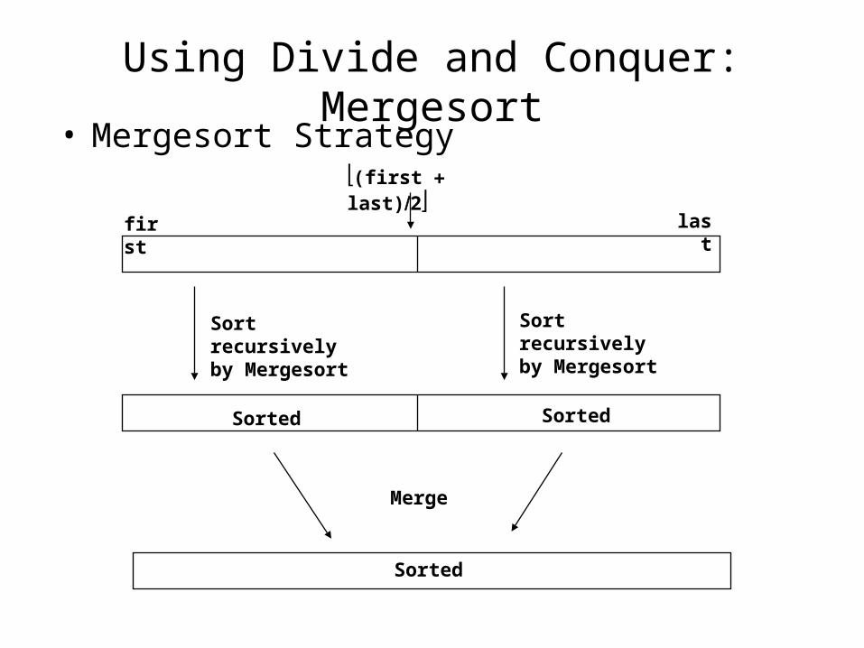
Using Divide and Conquer: Mergesort• Mergesort Strategy
Sorted
Merge
Sorted Sorted
Sort recursively by Mergesort
Sort recursively by Mergesort
first last
(first last)2
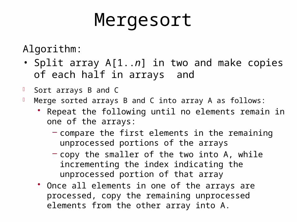
MergesortAlgorithm:• Split array A[1..n] in two and make copies of each half in arrays
and Sort arrays B and C Merge sorted arrays B and C into array A as follows:
• Repeat the following until no elements remain in one of the arrays:– compare the first elements in the remaining unprocessed portions
of the arrays– copy the smaller of the two into A, while incrementing the index
indicating the unprocessed portion of that array • Once all elements in one of the arrays are processed, copy the
remaining unprocessed elements from the other array into A.

Algorithm: MergesortInput: Array E and indices first and last, such that
the elements E[i] are defined for first i last.Output: E[first], …, E[last] is a sorted
rearrangement of the same elementsvoid mergeSort(Element[] E, int first, int last)
if (first < last)int mid = (first+last)/2;mergeSort(E, first, mid);mergeSort(E, mid+1, last);merge(E, first, mid, last);
return;
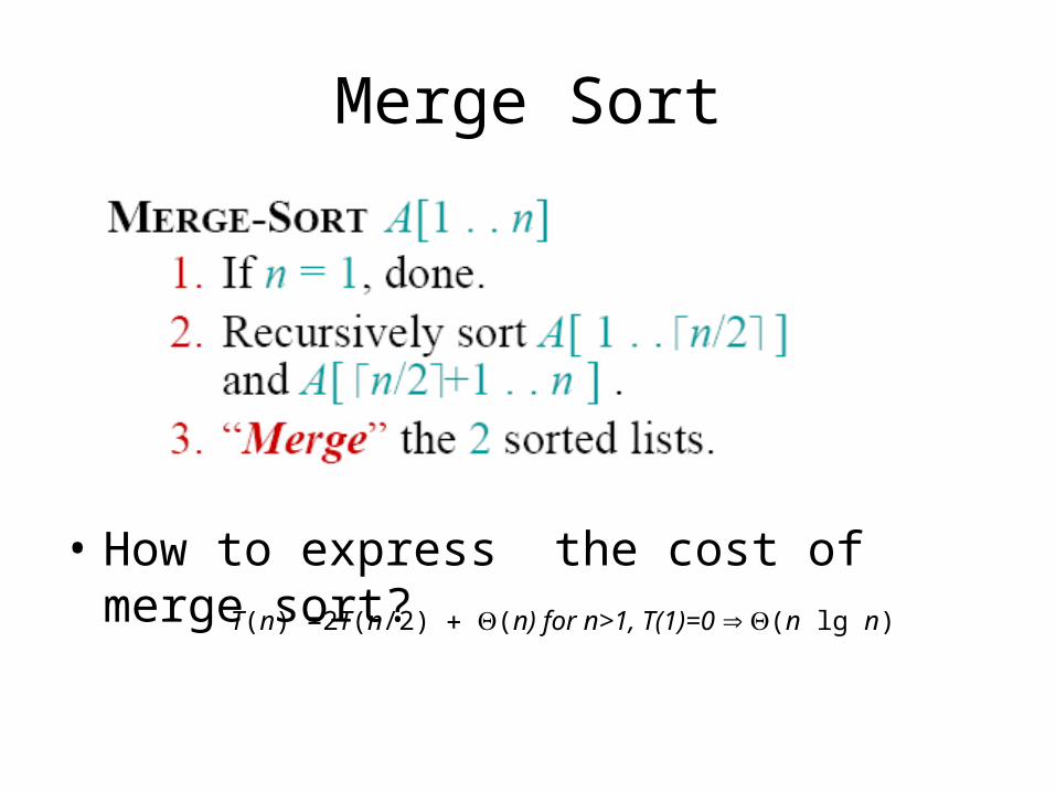
Merge Sort
• How to express the cost of merge sort?T(n) =2T(n/2) (n) for n>1, T(1)=0 (n lg n)

Merge Sort
1.Divide:Trivial.2.Conquer:Recursively sort subarrays.3.Combine:Linear-time merge.
# subproblems
subproblemsize
cost of dividing and combining

Efficiency of Mergesort
• Number of comparisons is close to theoretical minimum for comparison-based sorting: – lg n ! ≈ n lg n - 1.44 n
Space requirement: Θ( n ) (NOT in-place)
Can be implemented without recursion (bottom-up)
All cases have same efficiency: Θ( n log n)

Quicksort by Hoare (1962)• Select a pivot (partitioning element)• Rearrange the list so that all the elements in the positions before
the pivot are smaller than or equal to the pivot and those after the pivot are larger than or equal to the pivot
• Exchange the pivot with the last element in the first (i.e., ≤) sublist – the pivot is now in its final position
• Sort the two sublists recursively
• Apply quicksort to sort the list 7 2 9 10 5 4
p
A[i]≤p A[i]p

Quicksort Example• Recursive implementation with the left most array
entry selected as the pivot element.

Quicksort Algorithm• Input:
Array E and indices first, and last, s.t. elements E[i] are defined for first i last
• Ouput: E[first], …, E[last] is a sorted rearrangement of the array
• Void quickSort(Element[] E, int first, int last)if (first < last)
Element pivotElement = E[first];int splitPoint = partition(E, pivotElement, first, last);quickSort (E, first, splitPoint –1 );quickSort (E, splitPoint +1, last );
return;

Quicksort Analysis• Partition can be done in O(n) time, where n is the
size of the array• Let T(n) be the number of comparisons required by
Quicksort• If the pivot ends up at position k, then we have
– T(n) T(nk) T(k 1) n• To determine best-, worst-, and average-case
complexity we need to determine the values of k that correspond to these cases.

Best-Case Complexity
The best case is clearly when the pivot always partitions the array equally.
Intuitively, this would lead to a recursive depth of at most lg n calls
We can actually prove this. In this case – T(n) T(n/2) T(n/2) n (n lg n)

Worst-Case and Average-Case Complexity
• The worst-case is when the pivot always ends up in the first or last element. That is, partitions the array as unequally as possible.
• In this case – T(n) T(n1) T(11) n T(n1) n
n (n1) … + 1 n(n 1)/2 (n2)
• Average case is rather complex, but is where the algorithm earns its name. The bottom line is:
)lg(lg386.1)( nnnnnA

QuickSort Average-Case
S< : x < p p S> : x > p
n
i n – i –1
WLOG Assume: | S= | = 1. If it’s larger, it can only help!
T(n) = T(i) + T(n-i-1) + Q(n), T(n) = Q(1), for n=0,1.
Expected-Case:
T(n) = avei { T(i) + T(n-i-1) + Q(n) : i = 0 .. n –1 }
1n
0i
)n()1in(T)i(Tn1
)n()i(T1n
0in2
= Q(n log n)83

QuickSort Average-Case
0n,n)i(T2)n(Tn 21n
0i
1. Multiply across by n (so that we can subsequently cancel out the summation):
2. Substitute n-1 for n: 1n,)1n()i(T2)1n(T)1n( 22n
0i
3. Subtract (2) from (1): 1n,1n2)1n(T2)1n(T)1n()n(nT
4. Rearrange: 1n,1n2)1n(T)1n()n(nT 5. Divide by n(n+1) to make LHS & RHS look alike: 1n,
)1n(n1n2
n)1n(T
1n)n(T
n1
1n3
1)n(n1-2n ,
n)1n(T
)1n(Q ,1n)n(T
)n(Q
6. Rename:
0nfor 0
1n)1n(Q)n(Q n
11n
3
7. Simplified recurrence:
]0)0(T [ 0n,n)i(Tn2)n(T :2 Example
1n
0i
8. Iteration: 13
11
23
21
13
1131
13 )(2)0()( n
nnnnnnn nHQnQ
).nlogn(n3)n(H)1n(2)n(Q)1n()n(T 9. Finally:
nth Harmonicnumber
84

Summary of Quicksort
• Best case: split in the middle — Θ( n log n) • Worst case: sorted array! — Θ( n2) • Average case: random arrays — Θ( n log n)

Summary of Quicksort• Best case: split in the middle — Θ( n log n) • Worst case: sorted array! — Θ( n2) • Average case: random arrays — Θ( n log n)
• Considered as the method of choice for internal sorting for large files (n ≥ 10000)
• Improvements:– better pivot selection: median of three partitioning avoids worst case
in sorted files– switch to insertion sort on small subfiles– elimination of recursionthese combine to 20-25% improvement