ANALYSIS AND DESIGN OF A MAGNETIC BEARING

j

A N A L Y S I S A N D D E S I G N O F A M A G N E T I C B E A R I N G

Vladimir Soukup

B. Sc. (Electrical Engineering) Czech Technical University

A T H E S I S S U B M I T T E D I N P A R T I A L F U L F I L L M E N T O F

T H E R E Q U I R E M E N T S F O R T H E D E G R E E O F

M A S T E R O F A P P L I E D S C I E N C E

in

T H E F A C U L T Y O F G R A D U A T E S T U D I E S

D E P A R T M E N T O F E L E C T R I C A L E N G I N E E R I N G

We accept this thesis as conforming

to the required standard

T H E U N I V E R S I T Y O F B R I T I S H C O L U M B I A

June 1988

© Vladimir Soukup , 1988

In presenting this thesis in partial fulfilment of the requirements for an advanced

degree at the University of British Columbia, I agree that the Library shall make it

freely available for reference and study. I further agree that permission for extensive

copying of this thesis for scholarly purposes may be granted by the head of my

department or by his or her representatives. It is understood that copying or

publication of this thesis for financial gain shall not be allowed without my written

permission.

Department

The University of British Columbia Vancouver, Canada

Date

DE-6 (2/88)

Abstract

Magnetic bearings have recently begun to be employed in rotating machinery for vi

bration reduction, elimination of oil lubrication problems and prevention of failures.

This thesis presents an analysis and design of an experimental model of a magnetic

suspension system. The magnetic bearing, its control circuit and the supported ob

ject are modeled. Formulas are developed for the position and current stiffness of the

bearing and the analogy with a mechanical system is shown. The transfer function is

obtained for the control and experimental results are presented for the double pole one

axis magnetic support system.

i i

Table of Contents

Abstract i i

List of Figures v

1 I N T R O D U C T I O N 1

2 D Y N A M I C M O D E L O F M A G N E T I C B E A R I N G S 6

2.1 Introduction 6

2.2 Lifting Force of an Electromagnet 6

2.3 Stiffness of Magnetic Bearings 9

2.4 Mechanical Analogy of Magnetic Bearing 11

2.5 Mathematical Model of Magnetic Bearing 13

3 S O L U T I O N O F T H E D I F F E R E N T I A L E Q U A T I O N 15

3.1 Introduction 15

3.1.1 Critical Points of a System 16

3.1.2 Transformation of the 2nd Order to the l " Order Differential

Equations 17

4 L I N E A R I Z E D M O D E L O F M A G N E T I C B E A R I N G S 21

4.1 Introduction 21

4.2 Linear Approximation of an Electromagnetic Force 22

4.3 Linearized Model and the Transfer Function 23

iii

5 I M P L E M E N T A T I O N O F A M A G N E T I C B E A R I N G 26

5.1 Introduction 26

5.2 Velocity Transducer 27

5.3 Position Transducers 28

5.4 Power Drivers 31

5.4.1 Voltage Driver 31

5.4.2 Current Feedback 33

5.4.3 Current Driver 34

6 M E A S U R E M E N T S 36

6.1 Introduction 36

6.2 Double Ended and Single Ended Models 36

6.3 Electric Time Constant of the Electromagnet 38

6.4 Position Constant of the Hall Effect Sensor 39

6.5 Velocity Constant 39

6.6 Measurement of The Position Stiffness 41

.7 C O N C L U S I O N S 45

Bibliography 4 7

A P P E N D I X 49

iv

Lis t of Figures

1.1 Model for a Magnetic Suspension System 2

1.2 Radial Suspension of a Rotor 3

2.3 Coordinate System of the Double Ended Suspension System 7

2.4 The Electromagnet 7

2.5 Model of an Analogous Mechanical System 11

2.6 Characteristic Roots of a Second Order System in the Complex Plane . 13

4.7 Graphical Representation of Transfer Function Poles in the s plane . . . 24

5.8 Velocity Transducer 27

5.9 Resonant Circuit Measurement Method 29

5.10 Phase-Locked Loop 29

6.11 Voltage vs. Current in a Series RL Circuit 38

6.12 Measurement of the Velocity Constant 40

v

Chapter 1

I N T R O D U C T I O N

The idea of suspending a mechanical object in a magnetic field is not new. It spans

nearly 150 years back to the year 1842 when S. Earnshaw [1] developed a theorem

which states that a system using permanent magnets or electromagnets without control

of current is inherently unstable. His work was later followed by W. Braunbeck [2] and

others. Although Earnshaw was right, there are now magnetic suspension systems that

use both permanent magnets and electromagnets with controlled currents together

in that the permanent magnets are employed to carry all static loads whereas the

electromagnets are used just for control purposes to stabilize the system. These systems

are known as VZP (for " Virtually Zero Power "), because such an arrangement results

in minimal power requirements since they approach zero power consumption as a limit,

regardless of how much mass is suspended. This type of suspension system is especially

convenient in applications where space, weight and power are limited.

Now a magnetically suspended 1100 kg shaft capable of spinning at 10,000 rpm or

higher is becoming a commercial reality. Already such shafts turning at various speeds

are being used in grinding and polishing machinery, vacuum pumps, compressors, tur

bines, generators and centrifuges. Electronically controlled magnetic bearings offer two

major advantages: there is no mechanical wear and no frictional losses or lubrication

requirements.

In order to fully position a rotating shaft, a magnetic force must be applied along

five axes: two perpendicular axes at each shaft end and a fifth axis parallel to the

1

Chapter 1. INTRODUCTION 2

Figure 1.1: Model for a Magnetic Suspension System

shaft's rotational axis. A complete model [3} for such a suspension system resembles

a set of springs and dampers where each spring represents one electromagnet and is

shown in Fig.1.1. This thesis deals with analysis and design of just one axis control

(axial suspension). Once the control circuitry is developed and its characteristics found

satisfactory, it will be used in the remaining axes as well.

The electronic system is intended to control the position of the rotor by acting on the

current in the electromagnets on the basis of the signal from the position and velocity

sensors. The signal from the position sensor is compared with the difference signal,

which defines the rotor's nominal position. If the reference signal is zero, the nominal

position is in the centre of stator. By acting upon the reference signal, it is possible to

shift the nominal position of the shaft by up to half the air gap. The error signal is

proportional to the difference between the nominal position and actual position of the


Electromagnet

Figure 1.2: Radial Suspension of a Rotor

rotor in any given time. This signal is transmitted to the analog signal processing part

which produces a control signal to the power amplifier. The ratio of the output signal

to the error is chosen so as to maintain the rotor as precisely as possible at its nominal

position and to return it rapidly to the nominal position, with a well damped movement,

in the event of any disturbance. The servo system defines the stiffness and damping of

the magnetic suspension.

Practical radial suspension [4], as shown in Fig.1.2., is used on each end of the shaft.

In this arrangement there is no mechanical contact between rotor and stator. Rotor

size has little effect on the signal processing of the control circuit. Only the power

amplifier design depends on bearing capacity.

The time constants of typical electromagnets might be as large as several hundred

milliseconds and yet the magnet-amplifier combination must act as a closed loop con

trol system with a bandwidth of at least 10 kHz [5]. A fairly substantial reserve voltage


to force rapid current change in the electromagnet, in order to overcome the inductive

voltage, is therefore an essential feature in the design of DC power amplifiers for con

trolled DC electromagnets. This requirement can lead to large power dissipation and

low efficiences in quiescent operating conditions.

Switching amplifiers are much more efficient than linear amplifiers and only con

verters of this type are considered in this thesis. The switching amplifiers can cover

a wide range of power ratings from small applications, such as spindles for revolving

mirrors where very high rotating speed and high speed stability is required, to large

turbine generators where magnetic bearings do not require regular maintenance. High

frequency switching amplifiers (choppers), using pulse-width modulation to control a

duty-ratio of the switching element and thus electric current for the electromagnets,

provide an effective and economical solution. This is described in more detail in Chap

ter 5.

In order to modify the force-distance characteristic so that the current in the elec

tromagnet, and thus the force of attraction, decreases as the gap decreases (and vice

versa), some form of feedback control must be used. From physical laws governing the

equation of an electromagnet it becomes obvious that the system is highly nonlinear.

To analyze this system and to explore possible linearization techniques in the case

of a vertical arrangement of the magnetic bearing is the purpose of this thesis.

The chapters in the thesis are arranged to form logical blocks. The general case of

an electromagnet is discussed in Chapter 2, covering the derivation of equations for the

lifting force and position and current stiffnesses. The analogy to a mechanical system

is also briefly described. The differential equation governing the non-compensated, un

stable magnetic system is also derived here. Chapter 3 is focused more on the nonlinear

equation and finding the type of singularity, by using a linearized form of the equation.


Chapter 4 continues with the linearized equation and a transfer function of the uncom

pensated system is found. Chapter 5 describes the practical realization of the magnetic

bearing and gives an evaluation of different types of control. Some experimental results

are given which are supplemented by material in Appendix. Chapter 6 discusses the

measurement techniques, used to calibrate the actual model for the calculations and

computer simulation. Overall conclusions are presented in chapter 7.

Chapter 2

D Y N A M I C M O D E L O F M A G N E T I C B E A R I N G S

2.1 I n t r o d u c t i o n

In this chapter equations for the lifting force of an electromagnet and stiffnesses of the

double-ended axial magnetic suspension will be deduced. A simplified view of such an

arrangement and its coordinate system is introduced in Fig.2.3. Several assumptions

will be made and their correctness will be evaluated in the conclusions of this thesis.

2.2 Lifting Force of an Electromagnet

An equation for the lifting force of a single electromagnet [9] can be obtained from the

work done in the magnetic system to change the field energy as

F = —2lli (2-1)

where L is an inductance and x is an air gap of the electromagnet. For further analysis

a few assumptions are made:

• magnetic reluctance of the iron core of the electromagnet is negligible in compar-

ision to the reluctance of the air gap

• flux levels are well below saturation limits

• fringing and leakage effects are neglected

6

Chapter 2. DYNAMIC MODEL OF MAGNETIC BEARINGS

©

Figure 2.3: Coordinate System of the Double Ended Suspension System

For an electromagnet such as shown in Fig.2.4 the inductance is expressed as

L = Rm

COIL N rc/R/v.s'

CROSS- SECTION

A, A 2

Figure 2.4: The Electromagnet

Chapter 2. DYNAMIC MODEL OF MAGNETIC BEARINGS

where the magnetic reluctance R„

_d/2 + x , d/2 + x {d/2 + x).l 1 •n-m — - I = ( 1

VQA! fj,0A2 MO M i Ai and using

1 1 Ai + A2

-r + -r Ay Ai A\Ai

equation (2.3) can be written as

_ jd/2 + x) Ax + A2

Ho MM

Symbols used :

H [A/m]... magnetic field intensity

j4i,j42[m2]... cross-sectional area

B [T]... magnetic flux density

Ho [H/m]... permeability of free space

$ [Wb]... magnetic flux

L [H]... inductance

Rm [l/H]... magnetic reluctance

N... number of turns of the coil

x [m]... air gap

now the equation (2,4) can be substituted into (2.2), yielding

I ^ »oN2

( MA2 \ {d/2 + xyAr + A2'

and — = 2MQ7V2 AJA2

dx {d/2 + xy[A1 + A2'

The magnetic flux can be derived from the magnetic equation

Rm$ = Ni

Chapter 2. DYNAMIC MODEL OF MAGNETIC BEARINGS 9

as

Mil

and finally the force

As Ho, N, Ai, A2, are constants, equation (2.9) can be simplified to

i2

F l = K(d/2 + x)> (2-10)

and similarly

F2 = if -(d/2 - x) 2

1 ^ = ̂ M^rrr) (2.11) where Ai-\- A2

From the analysis done so far, it is obvious that the lifting force of an electromagnet

depends on two variables: the current i and the air gap x, and that the equation is

not a linear function.

2.3 Stiffness of Magnetic Bearings

Since there are two independent parameters that can change, position x and current i,

equation (2.10) can be used to define a position and current stiffness as

P O S I T I O N S T I F F N E S S :

2 K ^ ^ = - 2 K W T x ) - t = c o n s t - ( 2 - 1 2 )

C U R R E N T S T E F F N E S S :

Ki = -—• — 2K —— , x — const. (2.13) 01 (a/2 + x)2 v '


Partial derivatives dx, di are used rather then dx, di since the force F is a function

of two independent variables x and i.

The stiffness terminology was used here since the situation is analogous to a spring.

However, for the electromagnet the effective stiffness is negative; this reflects the phys

ical behaviour in which a positive displacement of the shaft -fx, from the top elec

tromagnet, decreases the attractive force. Conversely, an actual spring would apply

a force tending to restore the original position of the mass. The consequence of the

negative spring stiffness causes the system to be essentially unstable.

In the compensated system a closed loop control is used to stabilize the position by

changing the current and the effective stiffness.

Chapter 2. DYNAMIC MODEM OF MAGNETIC BEARINGS 11

2.4 M e c h a n i c a l A n a l o g y o f M a g n e t i c B e a r i n g

There is an analogy between an electromagnet and the mass-spring-damper mechanical

system [17]. The case of a mechanical system is shown in Fig.2.5.

Fig.2.5: (a) simple mass-spring-damper mechanical system (b) corresponding network

The end of the spring and the damper have positions denoted'as the reference position.

If a force fext is applied to the mass m it will result in a displacement x. This displace

ment must be balanced by an extension of the spring forcing the mass to the original

position. Fig.2.5(a) can be drawn into a network in Fig.2.5(b). According to Newton's

law, sum of the forces at each node must add to zero. There is only one node here and

the equation is

where x, x and x are the displacement, velocity and acceleration of the mass m, B

represents the damping and k is elastance or stiffness, which provides a restoring force

represented by the spring. Assuming thatm, B and k are constants and all initial

conditions are zero, the Laplace transform can be used yielding

Fext{s) = s2X{s)m + sX{s)B + X{s)k

and the transfer function between Fext(s) and the resulting displacement X(s) is

fext{t) = mi + Bx + kx

Fext{s) = m(s2 + s 1

m m


The expression

s* + a l + A = 0 (2.14) m m

is called the characteristic equation of the system from Fig.2.5. Its roots reflect the

behaviour of the system. Eq.2.14 can be compared to

s2 + 2Zwns + w2

n = 0 (2.15)

yielding bJr, B

2mu>r

( 2.16)

Location of 5 roots in eq.2.14 corresponds to the stability and dynamic characteristics

of the system.

In case of a single electromagnet with constant current any displacement of the

mass from the balanced position will result in further move either towards or from

the magnet. Thus the electromagnet with a constant current demonstrates a negative

stiffness k. This instability is also apparent from the location of roots of eq.2.14. (Fig

2.6.), due to the positive real root, in the s-plane. Lm

I

UNSTABLE. Re

Figure 2.6: Characteristic Roots of a Second Order System in the s - Plane

To achieve a stable magnetic suspension the current in the electromagnet must be

controlled, which will effectively change the negative stifness k to a positive value and

remove the positive root from the s-plane.


2.5 Mathematical Model of Magnetic Bearing

To obtain a mathematical model of the magnetic bearing an equation of motion is

used which, for any mechanical model, is Newton's law

Application of this law involves defining convenient coordinates to account for the body's motion, i.e. position, velocity and acceleration. A simplified arrangement

of the vertical magnetic bearing is shown in Fig. 2.3.

Here the total gap d is equal to the top plus bottom gap (in the state of equilibrium

d/2 and d/2). Fx, F2 are attractive forces of the top and bottom electromagnet.

The equation of motion can be written as

F = ma (2.17)

where

JP[N]. . . vector sum of all forces applied to the body in the system

a[ms - 2]... acceleration

^[ms -2]... gravity constant

m[kg]... mass of the body

d2x mlm =m9 + F2-F1 + Fl ext (2.18)

or by using d2x dt2 = x

as

m'x — mg + K i (2.19) {d/2 - x) {d/2 + x) ext


the term mg can be lumped together with F'txt as Fext and the equation can be written

as

" - K _ K *'l F e x t

X ~ m {d/2 - x) 2 m {d/2 + i ) 2 + m ^• 2 0^

The coordinate system is symmetrical around d/2 (as was shown in Fig.2.3), where d/2

is the origin of the new coordinate system. Thus x can vary in the range from -d/2 to

d/2, where d is the total air gap of both electromagnets.

Chapter 3

S O L U T I O N O F T H E D I F F E R E N T I A L E Q U A T I O N

1.1 Introduction

A function f is linear if:

/ ( x i + x j ) = / ( s i ) + / ( x 2 ) (3.21)

and for any real number a

f{ax) = af{x) (3.22)

Any other function is nonlinear.

Equation (2 .20) , obtained from the equation of motion, evidently does not meet

the above conditions. It is a nonlinear second order differential equation with time

invariant coefficients.

Since frequency response techniques and root locus diagrams are not applicable to

nonlinear systems, there is a need for a graphical tool to allow nonlinear behavior to be

displayed. The phase plane diagram, which plots velocity x(t) vs. displacement x(t),

is a convenient technique. Although it is applicable only to second order processes, it

can be used for higher order systems, which can be approximated by a second order

equation. The variation of velocity x(t) vs. displacement x(t) for a specific initial

condition is called a trajectory. A set of trajectories for several initial conditions is

called a phase portrait.

15

Chapter 3. SOLUTION OF THE DIFFERENTIAL EQUATION 16

Let E represent a nonlinear second order dynamic system [13], which has two

state variables x\, x2. The vector x = (x\, x2)T is an dement of the real two-dimensional

state space X or briefly x 6 X.

In the case where system E is time invariant and receives no input, x(t) is deter

mined by t, x(0) and E. Thus:

£(*,Xo) = x ( « )

and x(t) is called a particular solution for the system E.

The trajectory through any point x 6 X is denoted 7r(x) and is defined as

7r(x) = [x(t) | x(0)] = x, -oo < t < oo

The positive semi-trajectory 7T+ through x is defined

7T+(x) = [x(t) | X(0)] = X, 0 < t < OO

A point x 6 X is called a critical point of the system E if

E ( t , x ) = x

for every t €E R1

3.1.1 C r i t i c a l Po in t s of a Sys tem

Critical (singular) points of a system are points of dynamic equilibrium. They corre

spond to positions of rest for the system and may be stable or unstable. The significant

feature of a critical point is that all derivatives are zero. In other words, the derivatives

of the state variables are zero.


A critical point of the system £ is:

(a) stable if, given a circular region of radius 6 > 0 around the critical point, there

exists another circular region of radius e concentric with the 6 region, where e > 6,

such that every positive half trajectory starting in the 6 region remains within the e

region.

A solution x(t), originating at x0(t), t0 is stable with respect to the critical point x if:

(1) x(t) is defined for all t satisfying t0 < t < oo

(2) if | x 0 — x |< 6, for some positive constant <5, then there exists another positive

constant e such that | x(t) — x |< e, Vr G (£o,°°)

(b) asymptotically stable if, it is stable and if in addition, every half trajectory

satisfying the conditions in (a), reaches the critical point in the limit as t —• oo.

A solution is asymptotically stable to the critical point x if it is stable and in addition

lim | x(t) — x |= 0

Unlike linear systems, which have only one type of behaviour everywhere in the

phase plane, nonlinear systems can have many different types of behaviour in different

regions. If a linear approximation can be done in each region, then the knowledge of

the whole system can be obtained.

3.1.2 Transformation of the 2 n d Order to the 1" Order Differential Equa

tions

If the nonlinear differential equation cannot be easily integrated, then a linearized form


of the equation can be obtained by means of Taylor or MacLaurin expansion. Once

the linear form of the second order differential equation is available it can be rewritten

into a form of two coupled differential equations of the first order.

Starting with the original nonlinear differential equation (2.20) and assuming Fext-0

.. K x — —

m

„-2

(3.23) (d/2-x) 2 (d/2 + x)2

The expansion with respect to x will be made about point x = 0 (i.e. MacLaurin

expansion).

The current can be set to t'i = i2 = i (const.) and the linearized differential equation

will be derived:

x(x,i) « £(0,i) + 0 x

x(0, i) = K t

5

dx K i2

m m (d/2)' = 0

dx{0,i) _ 2K i2 2K i2

dx m (d/2)* m (d/2)' 32Ki2

md3

Thus the linearized equation will be:

i(x,i) 32Ki2

md3 -x

This equation can be written as a set of coupled differential equations and the character

of the critical point determined according to the following theorem:

Let E be a second order linear system described by the equation:

X = AX

A critical point occurs at

X = 0


and the type of singularity depends on the eigenvalues of the matrix A accordingly:

• real and negative A l 5 A2 indicate stable node

• real and positive A l 5 A2 indicate unstable node

• real A l 5 A2 of opposite sign indicate saddle point

• complex A x, A2 with a negative real part indicate stable focus

• complex Ai, A2 with a positive real part indicate unstable focus

• imaginary Ai, A2 of opposite sign indicate centre

Using the linearized second order equation and making the following substitution :

x — Xi

X\ = x2

yields

%2 Z2Ki2

md3

(3.24)

x2 = (3.25)

These two equations can be expressed in a matrix form:

X = AX (3.26)

where

(3.27)

A = an al2

\ ° 2 1 «22 J (3.28)


(3.29)

Example

Equations (3.24), (3.25) can be evaluated for one practical situation:

K = 15.006xl0-6

m = 0.683 kg

d = 0.003 m (i.e. top and bottom air gap 1.5 mm)

H = «2 = 2 A

Then the A matrix will be

( 0 1

A = ^ 72670 0

with eigenvalues +269 and -269. Here, the eigenvalues are real and of opposite sign

which indicates a saddle point.

Chapter 4

L I N E A R I Z E D M O D E L O F M A G N E T I C B E A R I N G S

4.1 Introduction

A great majority of physical systems are linear within some range of the variables.

However, all systems ultimately become nonlinear as the variables are increased without

limit.

A system is defined as linear in terms of the system excitation and response. In

general, a necessary condition of linearity was given in the previous chapter by eq.(3.21)

and (3.22). The physical meaning is as follows:

when the system at rest is subjected to an excitation xi{t), it provides a response

yi(t). Furthermore, when the system is subjected to an excitation x2(t), it provides

a corresponding response y2(t). For a linear system,it is necessary that the excita

tion xi(t) + x2(t) results in a response y^t) + y2[t). This is called the principle of

superposition.

Furthermore, it is necessary that the magnitude scale factor is preserved in the

linear system. Again, consider a system with an input x{t) which results in an output

y{t). Then it is necessary that the response of a linear system to a constant multiple a

of an input x{i) is equal to the response to the input multiplied by the same constant

so that the output is equal to ay{t). This is called a property of homogenity.

21

Chapter 4. LINEARIZED MODEL OF MAGNETIC BEARINGS 22

4.2 Linear Approximation of an Electromagnetic Force

In the case of the magnetic bearing, it was shown in Chapter 2, that the equations

describing the system are highly nonlinear. Since, for a nonlinear system the principle

of superposition does not hold, the Laplace transform cannot be used and a transfer

function cannot be defined. It is very difficult to obtain some useful information about

the system and to control it by using classical control methods.

The force-distance characteristic (Appen. p.54) shows that the measured charac

teristic resembles a straight line in the range of interest (i.e. <0, 3>mm). Since the

magnetic bearing is designed to operate at a fixed point (d/2 = 1.5mm), the system is

clearly a good candidate for linearization at that point. The linear model then repre

sents behaviour of the system to a small signal or perturbation from the equilibrium

point.

A nonlinear equation can be expressed in a Taylor expansion about a point x0 or sim

ilarly in a McLaurin expansion about the point x0 = 0. As the equation of the lifting

force is a function of two variables (x,i), the linearized equation will be:

the linearization can be illustrated by placing a tangent plane onto the nonlinear surface

f(x,i) in the point i 0 , t'o.

The lifting force of an electromagnet can be linearized about point (x0,i0) as above

eq.(4.33). The forces F x , F2 were found in Chapter 1 to be

will be:

F{x,i) « F ( io , t 0 ) + dF{x0, t'o) 6\F(x 0,t 0) .

L x _) 1 L t

dx di (4.33)

K (4.34)

F 2 = K ' 2

(d /2-x) 2 (4.35)


The linearized form of the forces Fi, F2 about an equilibrium point x 0 = 0 and i 1 0

(resp.1'20)

Note that +2 and +i represent increments of the displacement and current.

4.3 Linearized Model and the Transfer Function

Now, the equation of motion

m i = F2 - Fi + Fext

can be written, using linearized forces as

(4.38)

A negative sign in (-i) means a decrease of current in the top coil (F{) as an opposite

of the increase (+i) of current in the bottom coil (F2). It is assumed that | + t | = | — t |

in both coils. In a steady state the shaft will be in a stable position between the two

electromagnets. The forces Fi, F2 will provide a resulting steady state force (due to

bias currents i'i0 and t 2o) which will compensate weight of the shaft (mg is part of Fext):

(d/2)2 (d/2)

The resulting equation using the stiffnesses (eq. 2.12, 2.13) will simplify to

mi = —Kxx — Kit (4.39)


Try,

-te

Figure 4.7: Graphical Representation of Transfer Function Poles in the s plane

where

tf.fO.iWa,) = 2Kj^ + 2K- l™ (d/2Y (d/2)*

Ki{0,i10,i20)=2K- + 2K-(«f/2)» (d/2)'

Now, the magnetic bearing can be approached as a linear system with small per

turbations of current i, as an input and the air gap x, as an output. In order to

express the transfer function (i.e. output x to input i), the equation of motion must be

transformed from the time domain to the 5 domain by means of the Laplace trans

formation. Suppose that the initial conditions are all zero and there is no damping;

then the equation (4.38) can be transformed into the s domain by means of Laplace

transformation as

s2

X{s)m = -KxX{s) -KJis) (

4

-4 0

)

Both Kx and K, are negative so the mass simply accelerates to the surface of the


electromagnet. Thus no electromagnet by itself can operate as a bearing. Solving the

equation of motion for the ratio X(s)/I(s) gives

X(s) -Ki/m 1(a) a 2 + Kx/m

(4.41)

where Kx and K , are negative values. Thus the roots of the system equation are +y

and —\[^- . Due to the the positive root the system is unstable.

This is the case of a negative spring compared to a genuine spring (with no damping)

where its roots would be both imaginary +jyf^ and located on the imaginary

axis symmetrically to the origin. In that case there would be undamped oscillations

with a natural frequency of [K~X

V m

And in a case with added damping the poles would be complex conjugates placed in

the left half plane, so that the oscillations would cease in a finite time. The graphical

representation is shown in Fig.4.7.

Chapter 5

I M P L E M E N T A T I O N O F A M A G N E T I C B E A R I N G

5.1 Introduction

Based on the theoretical analysis in Chapters 1, 2, 3 and the resulting linearized model

in Chapter 4, several variants of the one axis magnetic suspension control circuits were

built and tested for stability and reliability.

An evolution of the control circuitry followed practical experience and gained insight

into the problems. After experimenting with different sensors and power drivers a

simple, stable and reliable controller was constructed and is presented in this thesis.

Three different ways of controlling the electromagnets were investigated and built. The

comparison of their functions and the evaluation of results are discussed later in the

conclusions.

The most critical part of any system is its interfacing with the physical environment

i.e. the input sensors. The system developed here uses both position and velocity

transducers and the quality of signals produced by them is very critical for the whole

system. Experiments with substitution of the velocity signal by differentiating the

position signal were also performed. The resulting lead forward compensator could not

be practically used here, mainly because of the position signal quality. Any noise in

the position signal is emphasized after differentiation. For this reason both velocity

and position transducers are normally required in practice. A procedure for designing

a lead compensator from a root-locus diagram is presented in the Appendix.

26

Chapter 5. Implementation of a Magnetic Bearing 27

This compensator was tested experimentally, but the results confirmed the need for a

separate velocity signal.

This chapter presents the evalution of a practical design for the velocity and position

sensors and discusses the design of a practical power circuit.

5.2 Velocity Transducer

The original velocity transducer consisted of an air coil with a permanent magnet

connected with the shaft as shown in Fig.5.8(a). The resulting velocity signal was very

COIL

1 1

P p

N »S

COIL

(b)

Figure 5.8: Velocity Transducer

small and sensitive to any external magnetic disturbance. A new transducer was built

and it is shown in the same figure in (b). In that new design the coil is magnetically

shielded by a ferromagnetic case which forms part of the magnetic circuit. The magnetic

field is formed by a permanent magnet in the middle of the sensing coil. This way the

resulting output voltage is proportional to axial velocity while practically insensitive

to a radial movement. Since the gap between moving plate and the coil is very small,

no noise is induced and the signal is of a very good quality.


The voltage induced in the coil is

d$ v = N-j-

dt

where N represents number of turns of the coil and ^ is a change of magnetic flux,

by change of the magnetic reluctance of the magnetic circuit.

The output voltage of the transducer can be easily increased either by increasing

number of turns N or by adding a small amplifier close to the transducer: (as was done

here).

5.3 Position Transducers

Several methods were used to sense the displacement of the shaft, with different results.

Resonant C i r c u i t

A circuit consisting of a series arrangement of a coil L and a capacitor C was used in

this method. A frequency generator was used to produce a sinusoidal signal with a

frequency set on the side of the resonant curve. A change of inductance L then results

in a change of the output voltage across the resonant circuit LC. The high frequency

output signal is then processed by a peak detector to provide a DC voltage. This

method did not provide a stable, reliable signal. One reason was that the frequency

generator was not very stable and any change in the frequency or the amplitude added

an unwanted offset which required manual correction. Also since the peak detector

provides an "envelope" of the detected signal, any outside disturbance is automatically

included in the resulting signal.


tt

f V

Figure 5.9: Resonant Circuit Measurement Method

Frequency Detector

In this circuit the sensing coil L forms a part of an oscillator [6] of frequency

2TTVLC

Thus as the inductance is changed by an axial displacement of the shaft the resulting

change in frequency can be detected by a phase detector. A convenient solution [7],

[8];provides a Phase-Locked Loop (PLL) circuit, which operates as following: a phase

LPF.

CONTROL VOLTAGE

Figure 5.10: Phase-Locked Loop

detector compares two input frequencies and the output is a measure of their difference.

If they differ in frequency, it gives a periodic output at the difference frequency. If UN


does not equal /vco» the phase-error signal, after being filtered and amplified, causes

the VCO frequency to deviate in the direction of fjN- The VCO will quickly "lock" to

///vr, maintaining a fixed phase relationship with the input signal. The filtered output

of the phase detector is a DC signal, and the control input to the VCO is a measure of

the input frequency. A phase-lock loop is shown simplified in Fig.5.10,

After initial difficulties with the low pass filter, the PLL worked well, but yet the

long-time stability was not sufficient. The resulting DC output signal provided a volt

age change of about 0.2V for the full gap range. This signal, compared to a reference

voltage, results in an error signal which can be further amplified.

Hall Effect Sensor

This signal is of a good quality with long term stability and requires minimal additional

processing. This technique was therefore used in all further experiments.

The disk, connected to the shaft and forming a part of the velocity transducer,

was also used to produce position information. This was done by placing a Hall effect

sensor on the top of the permanent magnet measuring the flux density B of the resulting

magnetic field. The only drawback, which is the temperature sensitivity, can be solved

by placing the sensor further from the heat source. It could be also improved by

employing an electronic compensation technique, but in this case it was not necassary.

All the circuits listed in the Appendix use this type of sensor. Although the air

gap - output voltage characteristic is nonlinear, as shown on p.54, it can be considered

linear over the range of interest (air gap 0 - 3mm).


5.4 P o w e r D r i v e r s

Once the signals are detected and processed, they form a control signal for the power

drivers. Two types of power drivers [9], can be used for the magnetic bearing.

A class A chopper (one quadrant) is shown on p. 66 . This circuit can decrease the

output current, if desired, by effectively applying zero voltage across the electromagnet

(i.e. using only the +V.+I quadrant).During that (off) time the current continues to

flow through the freewheeling diode.

A class D chopper (two quadrant) is shown on p.67. Its advantage is that it can control

the output current even further, by applying full negative supply voltage across the

electromagnet, while the output current freewheels through the power supply. This

could produce improved dynamic performance at increased cost. However, in the dou

bly excited system analyzed in this thesis, a fast rise in force in either direction is

possible even if only one quadrant controllers are used. Therefore, for simplification,

this was the only type of circuit considered here. The resulting system performed satis

factorily, but the investigation of two quadrant controllers can be carried in the future.

5.4.1 V o l t a g e D r i v e r

The first control circuit that was designed and built was simple, yet fully operational

and gave us the "feel" of a magnetic suspension. The name voltage driver is used here

to refer to a voltage output of the amplifier which is the result of input signals, position

and velocity. The block diagram is shown in the Appendix on p.58. The relationship

between the voltage applied across the electromagnet V(s) and the resulting current

I(s) is expressed, using lumped parameters R and L as:

V(s) = sLI{s) + RI{s) = I{s){sL + R]


and V(s)

I(s) =

where r = j- is known as the electric time constant. The meaning of the above equation

is that the current I(s) is not linearly proportional to the voltage V(s), but it is lagging.

Furthermore T depends on the air gap of the electromagnet. Since the linearized model

is already being used, r can be measured for the specific air gap and considered constant

within a small range. The method of an air gap measurement is discussed in Chapter

6 and, for an air gap of 1.5mm, r equals 15.6ms. The transfer function of the closed

loop system is derived by consequent simplifications analogous to those, used on pp.62 - 65 for a current driver. Use of that procedure yields the transfer function

i KPK, xjfi s 2m •+• sK,Kv + KpK,H — Kz

where

K, ^(Ka + K,!)—!— ST •+- 1

and

Kx = Kxi + Kz2

From Chapters 2 and 3 K, and Ks are known to be the current and position stiff

nesses and are calculated in A43 for a fixed gap 1.5mm and several values of current.

The electric time constant can be expressed from

1 _ 1 sr + 1 ~ r(s + -J)

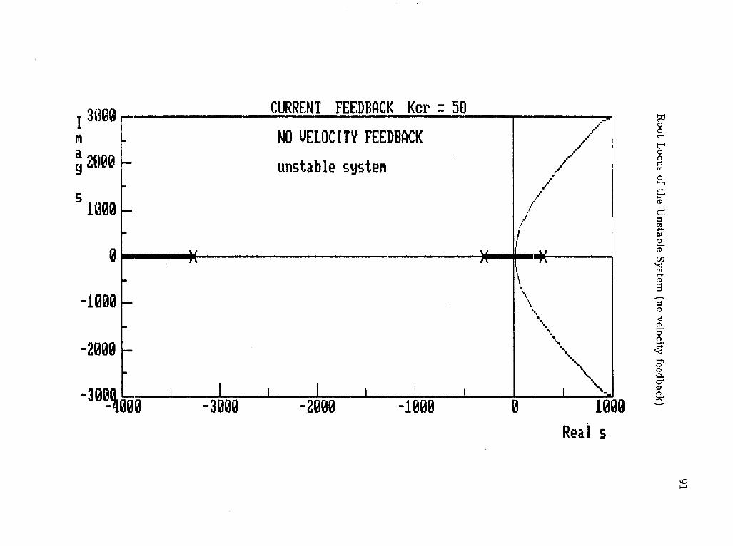
as a pole s=-* in s - plane of value -64.10. Its effect can be seen in the root locus where

being close to the origin it constitues a dominant pole pushing the root locus branch

to the right half plane. Thus with no velocity feedback the system is unstable for any

value of position gain Kp.


For an illustration several root locus plots are shown on pp.85 - 88. A region of stability

is investigated for different values of the velocity gain Kv. Only a narrow range of Kp

demonstrates a stable state. This is in full agreement with the practical experience,

where the system had to be frequently adjusted. Since this arrangement could not be

kept stable over a longer time, it was really of no practical use and it was abandoned.

5.4.2 Current Feedback

The situation with the unwanted dominant pole, due to the electric time constant, can

be improved by introducing current feedback. As an example let

57 + 1

to be a transfer function of the electromagnet (i.e. I0ut/Vin), resulting thus in a pole

s=-^. Let Keur be a gain of an amplifier connected in cascade with the electromagnet.

Then by closing a negative unity feedback (see A6) the new transfer function will be

G= HT + l _ '•••cur 1 + 7rTl *T+l+Kcur

and the new pole will be at 1 + Kcur s =

T

Thus by using current feedback the unwanted significant pole can be moved further

from the origin into the left half plane and become less significant for the dynam

ics of the system. The model shown in the block diagram on p.59 is very similar to the

voltage driver diagram. The current feedback can be implemented either only on one

electromagnet (p.73) or on both ends (pp.74 - 75), where both currents are monitored

independently.


The transfer function has again the same general form as with the voltage driver,

only the Kt is different, since it cointains the local current feedback loop:

^ " " • t r + l

1 + * c „ r ^

5.4.3 Current Driver

It becomes obvious that by increasing the current loop gain without limit the original

time constant s = approaches -infinity. This practically means that the electric time

constant becomes negligible and can be omitted. Thus the current driver is actually a

transconductance amplifier with the transfer function

hut . —— = const. Yin

By employing a current source the system will become much easier to stabilize and

will remain stable both over a wider range of control parameters Kp, Kv and system

parameters (which may drift over an extended period of time).

A block diagram of such a system and its simplification process is shown in detail

on pp.60 - 65. The system used here will have, under normal operating conditions, a

zero input (x,„) and is referred to as a "zero tracking regulator". For a measurement of

dynamic characteristics it is convenient to observe the system response to a standard

arbitrary input, such as an unit impulse, unit step, sinusoidal or square wave input

which may represent both a driving function or a disturbance. As an example a sudden

load being applied to the magneticaly suspended rotor will result in a precendented

reaction. This disturbance can correspond either to a position disturbance x,„ or to a

force disturbance Fext. Thus by introducing the transfer function as — or is pos-* m f a t

sible. The correspondence between those two functions becomes clear from the block

diagram on pp.64 - 65. The only difference is a scaling factor.


The equations i KPK, (5.42)

s*m + sK,Kv + KPK,H - Kx

or x Kp K, [ m (5.43) in s 2 + sK.KJm + (tfptf.tf - Kz)/m

can be compared to the standard form of a second order differential function :

where C is a constant and Kx is the position stiffness calculated from eq.2.12 and listed

on pp.98 - 99.

An examination of the coefficients in the denominators provides an important insight

into the change of an unstable (negative) spring situation to a real spring situation with

a positive (restoring) force type. By increasing the position gain K p , the stiffness of the

bearing can be increased (theoretically to infinity). Practically this is not possible be

cause of nonideal position and velocity signals. Also the damping of the system £

depends on the velocity gain Kv.

The boundary of the theoretical stiffness and practical limitations due to a nonideal

physical world will now be investigated.

C (5.44) a1 + 2£w ns + ul

2mwn

Chapter 6

M E A S U R E M E N T S

6.1 I n t r o d u c t i o n

In order to calibrate the model of one axis double ended vertical bearing, several mea

surements had to be done. A brief description of each measurement technique, together

with the results obtained, are presented in this chapter.

The model used for the measurements was the current driver system with:

top and bottom gaps .d/2 - 1.5 [mm]

mass of the shaft m = 0.683 [kg]

gravity constant g = 9.81 [m/s2]

The other parameters were being changed for different measurements and they are

specified in the appropriate place in the text.

6.2 D o u b l e E n d e d a n d S i n g l e E n d e d M o d e l s

All the analysis of the magnetic bearing so far was concerned with the "double ended''

model, mainly for reasons of practical use and also because the equations obtained

can be easily changed to describe the single ended model (i.e. using only the top

electromagnet) by setting t 2 = 0 and thus (=> F2 =0).

Although the single ended model is of little use for the practical bearing, it can

be utilized for a convenient calibration of the model. As mentioned earlier, a number

36

Chapter 6. MEASUREMENTS 37

of simplifications were used (those concerned with fringing, leakage, saturation and

magnetic reluctance of iron ). In order to obtain a practical model for further analysis,

it must be checked that the model does not stray too far from reality.

A theoretical constant K was calculated in section 2.2. This can be checked ex

perimentally as follows. The current in the bottom coil is set to zero and the current

required by the top electromagnet to maintain a particular gap is then measured. The

gap, which will be used in the constructed bearing is the most important. The equation

of motion will simplify to

m i = mg — F x = 0 (6.45)

so that

Fi = mg

K —-, — = TOO (d/2 + z)»

(where d/2 is the gap) and since the values of mass m, gap and current can be

easily obtained. A corrected value of the constant K can be thus determined from the

equation:

t2

In the case of the model used with Kp = 150 and Kv = 0.6, the current z'i was found

to be 1.19 [A], corresponding to a force of 6.73 [N]. For further values of the airgap see

A51.

Thus a new constant of the electromagnet was found to be:

K = 10.646 * 10"6


This corresponds to a 29% decrease from the originally calculated value 15.005* 10 6 .

All the calculations in this thesis are based on this new, corrected value.

6.3 Electric Time Constant of the Electromagnet

A series combination of L and R is used here to represent the electromagnet. Thus by

solving the equation for current as a function of applied unit step voltage we obtain

« = Imax{l - C ' ) (6.47)

where

I max — D

represents a steady state value of a DC current. This equation can be evaluated for

t = T, where r is the electric time constant as denned earlier in section 5.4.1 to yield:

t = / m ox ( l - e~r) = / m a i ( l - e"1) = 0.632/maI

0 T T N ^ ^ Figure 6.11: Voltage vs. Current in a Series RL Circuit

Now, using a low frequency square wave generator and a power amplifier, the output


voltage is applied across the electromagnet (fixed airgap) and the resulting current is

displayed (by means of a current transducer) on an oscilloscope.

In the practical case /m a i=3.5 [A] and 63.2% of which was 2.21 [A]. The time

corresponding to this current level was found to be:

r = 15.6[ms]

6.4 P o s i t i o n C o n s t a n t o f t h e H a l l E f f e c t S e n s o r

The characteristic, i.e. the output voltage as a function of the air gap, of the Hall effect

sensor was measured and is shown in A l . It can be seen that the function, in the range

of <0, 3> mm, can be substituted with a straight line of appropriate slope. The slope,

and thus the transfer function, was found to be:

H = 110[V/m]

6.5 V e l o c i t y C o n s t a n t

Similarly, the velocity sensor transducer had to be calibrated. The appropriate part of

the block diagram, together with x = x(t) and x = x(t) is shown in Fig.6.12. Position

and velocity response for a simulated impulse input and Kp = 150, H = 110 and Kv

= 0.6 (underdamped case), were displayed on an oscilloscope simultaneously. The fol

lowing can be written

x = Xmaxsinujt

u = — = 2nf T

where w [rad/s] is radian frequency, T [s] is the period and f [Hz is cyclic frequency.

Chapter 6. MEASUREMENTS

X 1 x

/5-0

4 ®* K ? - ^ - T

2.7

110 Figure 6.12: Measurement of the Velocity Constant

and for velocity

dx X = — = 0jXmaxCOSUt = XnaxCOSUt

at

The following data were obtained:

T = 28 [ms], so that:

u> = 224[ra<i/s]

X^ = 8 V « 0.485mm (i.e. 8/150/110) yielding :

KPabs = 16495[F/m]

Similarly:

Xmax = 12 V and

Xmax = w l m 0 1 = 224 * 0.485 * 10~3 = 0.1086 [m/s]

12/0.1086 = 110.5 [V/m/s] and 110.5/2.7 = 40.93 so that:

KVab, = 40.93\V/m/s}


6.6 Measurement of The Position Stiffness

As outlined briefly in 5.4.3 (page 34), a technique simulating an unit impulse response

[10],[11],[12] was used here in order to obtain the stiffeness values for the closed loop

suspension system. An analogous system to the magnetic bearing is the mechanical

mass-spring-damper system, as discussed earlier, where the input R(s) and output X(s)

are related through the transfer function T(s) r(5)

= fw =

+ + <6

"8

> The poles of the above equation are

* = -fw„ ± j uny/l - (2

If the unit impulse 6(t) is used as an input then the response of the system X(s) will

be equal to T(s)

X(s) = T(s)

since the Laplace transform £6(t) = 1

The transient response in the time domain can be obtained by using inverse Laplace

transform of X(s) (= T(s)):

x(t) = L-lX{a) = —e-^sinu.t = 4 e - ^ ' « n ( W r i V T q j ) t

where

u>„ . . . natural radian frequency

ojd ... damped radian frequency

£ . . . damping ratio

a . . . damping coefficient

r . . . time constant of the system


and the basic equations:

= un^l i2 - 1

a = (wn

_ 1

a

£ = sin'16

0 = tan'1^

As £ decreases, the poles approach the imaginary axis and the system becomes increas

ingly oscillatory.

It is common to take several performance measures from the transient response to

a step input. The swiftness of the response is measured by the rise time Tr and the

peak time T p . For underdamped systems with an overshoot, the 0-100 % rise time is

a useful index. If the system is overdamped then the peak time is not defined and the

10-90 % rise time is normally used.

The similarity with which the actual response matches the step input is measured

by the percent overshoot, P.O., and the settling time, T s . The settling time, T s , is

defined as the time required for the system to settle withtin a certain percentage of the

input amplitude. For a second order system with a closed-loop damping constant £,

the response remains within 2 % after four time constants.

In practice a demand for a fast response yet with an overshoot of less then 5 % can be

matched by the minimum damping ratio of 0.707 with a resulting overshoot of 4.3 %.


The stiffness of the closed loop compensated system was obtained from the tran

sient response to a simulated unit impulse (mechanical impulse).

The natural radian frequency of the undamped system un was obtained from the os

cilloscope, while position gain Kp and velocity gain Kv were set so that the system

produced a sustained periodic oscillation. The damped radian frequency uj was ob

tained in a similar manner for different settings of Kp and Kv. Pictures were taken

from the screen of a storage oscilloscope and they are shown together with computer

simulated responses in Appendix pp.78 -83.

parameters measured values calculated values

K„

100 0.6 222 227 0.209 12900

100 0,7 209 227 0.209 12900

100 2.7 122 227 0.844 12900

150 0.9 326 336 0.242 48600

150 1.5 290 336 0.505 48600

150 2.7 140 336 0.909 48600

150 5.0 97 336 0.957 48600

£ = l - ( ^ ) 2 Kcomp = ' un • mu\

where Keomp is the stiffness of the compensated system.


As can be seen from the table the natural radian frequency w„ and the effective

stiffness K depend on the position gain K p , whereas the damping ratio £ and thus the

damped radian frequency depend on the velocity gain Kt,.

An expression for a steady state error (i.e. in this case it would be the steady state

displacement of the shaft if a constant force is applied) can be calculated, using the

steady-state or the final-value theorem:

limx(t) = UmsX(s)

the situation corresponds to a unit step being applied

limsX(s) = lim s

s{s* + 2&n + W 2 )

in case of the bearing it would be

1 m KVK FH—KX KPKSH

m

Chapter 7

C O N C L U S I O N S

The goal of this thesis was to analyse and design a practical one-axis double-ended

magnetic bearing. A complete analysis of the vertical arrangement was done, forming

a good base for further investigation. This included: equation of motion, equation for

the lifting force of an electromagnet, general expressions for stiffnesses, linearized form

of the force and finally a model for small signals (perturbations).

From the analogy with a mechanical system, the equation for the position stiffness

of the closed loop suspension system was derived and measured, using a simulation of

the unit impulse response. The results were found to be in good agreement with the

calculated values. The formula for a steady-state error, in the case of a unit step input

(i.e. a case of a suddenly applied load) was derived from the final value theorem. A

good insight into the system properties was obtained by using the root-locus plots and

an example af a complete procedure for synthesizing any type of cascade compensator

is presented in the Appendix.

A high importance was placed on the position transducer by analyzing its role

in the ultimate bearing stiffnesses. This is still a vast area to be investigated. By

comparing different types of transducers the Hall-effect transducer was found to be

a very convenient type for its good quality output signal with no further processing

necessary.

The key goal, which was to actually build a circuit that will perform the control

function, was achieved. The identical circuitry can be now made for those remaining

45

Chapter 7. CONCLUSIONS 46

four axes to completely suspend the rotor. Further investigation may still be necessary

in the multi-axes suspension case, if a possible cross coupling would occure.

The future of magnetic bearings is still open which is obvious from a number of

papers being published. Some other types of position transducer candidates would

be capacitance sensors and optoelectric sensors. Further explorations of this topic

promises to pose an interesting challenge.

47

Bibliography

[l] Earnshaw, S., On the nature of the Molecular Forces which regulate the Constitu

tion of Luminoferous Ether, Trans. Camb. Phil. Soc, 7, pp. 97-112 (1842)

[2] Braunbeck,W., Free Suspension of Bodies in Electric and Magnetic Fields,

Zeitschrift fur Physik, 112, 11, pp. 753-63 (1939)

[3] Habermann, W., Liard Guy L., Practical Magnetic Bearings, Societe de Mecanique

Magnetique, France; IEEE Spectrum, September (1979)

[4] ACTIDYNE - Application of Active Magnetic Bearings to Industrial Rotating Ma

chinery, Societe de Mecanique Magne'tique, France

(5] Jayawant, B. V., Electromagnetic Levitation and Suspension Techniques, Edward

Arnold Publishers (1981)

[6] Fogiel, M . , The Electronic Problem Solver, Research and Education Association,

New York N.Y. (1982)

(7] Horowitz, P., Hill, W., The Art of Electronics, Cambridge University Press (1983)

[8] Geiger, Dana F., Phaselock Loops for DC Motor Speed Control, Wiley ic Sons, Inc.

(1981)

[9] Dewan, S. B., Slemon, G.R., Power Semiconductor Drives, Wiley &: Sons, Inc.

(1984)

(10] Dorf, R.C., Modern Control Systems, Addison-Wesley (1982)

48

[11] Di Stefano J.J., Feedback and Control Systems, McGraw-Hill, 1976

[12] Franklin Gene F., Powell David J., Feedback Control of Dynamic Systems,

Addison-Wesley, 1986

[13] Leigh J. R., Essentials of Nonlinear Control Theory, Peter Peregrinus Ltd., Lon

don, U.K., 1983

[14] SIGNETICS - Linear Circuits Catalog, 1986

[15] UNITRODE - Linear Circuits Catalog, 1986

[16] Haberman H. et al., IEEE Spectrum, Sept. 1979, p.26

[17] D'Azzo John J., Houpis Constantine H., Linear Control System Analysis and De

sign, McGraw-Hill, 3rd Edition, 1988

49

APPENDIX

50

List of Appendix

1 Output Voltage of the Hall Effect Sensor vs. Air Gap 54

2 Output Current vs. Input Voltage of the Current Driver using 3843

Integrated Circuit 55

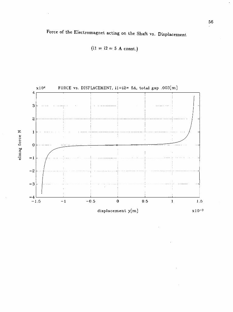
3 Force of the Electromagnet acting on the Shaft vs. Displacement (il =

i2 = 5 A const.) 56

4 Force vs. Displacement (calculated, 1st order approximation and 3rd

order approximation) 57

5 Block Diagram for Small Signal with linearized Force (Voltage Driver) . 58

6 Block Diagram for Small Signal with Linearized Force (Current Feed

back) 59

7 Basic Block Diagram of a Magnetic Bearing (Current Driver) 60

8 Block Diagram with Linearized Force (Current Driver) 61

9 Block Diagram for Small Signal with Linearized Force (Current Driver) 62

10 Simplification 1 (Current Driver) 63

11 Simplification 2 (Current driver), Simplification 3 (Current Driver) . . . 64

12 Simplification 4 (Current Driver) 65

13 Class A Chopper (one quadrant switching amplifier) 66

14 Class D Chopper (two quadrant switching amplifier) 67

15 A Saw Wave Generator for the Comparator Circuit 68

16 Comparator Circuit as a Generator of Control Signals for the D Class

Chopper 69

17 D Class Chopper (two quadrant switching amplifier) 70

51

18 Analog Part of the Control Circuit for the Magnetic Bearing (position

and velocity signals) 71

19 Simple A Class Chopper (Voltage Driver) 72

20 Simple A Class Chopper (Current Feedback) 73

21 A Class Chopper (Current Feedback) 74

22 The Complete Control Circuit (Current Driver) 75

23 Block Diagrams of Integrated Circuits 5561 and 3842 76

24 Impulse Response of a Second Order Linear System (for different values

off l 77

25 Impulse Response of the Single Axis Magnetic Bearing 78






31 Measured Stiffnesses of the Compensated Magnetic Bearing 84

32 Root Locus of the Stabilized System using a Voltage Driver 85




36 Root Locus of the Stabilized System using a Current Feedback 89

37 Root Locus of the Stabilized System using a Current Feedback 90

38 Root Locus of the Unstable System (no velocity feedback) 91

39 Root Locus of the System (without the velocity feeback) using a Lead

Cascade Compensator 92

40 RC Network Synthesis for a Feedback Amplifier 93

52

41 Root Locus of the Stabilized System using a Current Driver 96

42 Root Locus of the Stabilized System using a Current Driver 97

43 Calculated Values of Forces and Stiffnesses for the Uncompensated Sys

tem 98

53

Symbols used in the Appendix:

K t ...velocity gain (adjustable)

K p . . .position gain (adjustable)

K c u r . . . current loop gain (adjustable)

K e . . .system constant (-0.321 A/V)

K,; . . . converter constant (+0.5, -0.5)

H . . . Hall sensor constant (110 V/m)

K , . . . current stiffness of the uncompensated system (calculated)

K, . . . position stiffness of the uncompensated system (calculated)

T . . .electric time constant of the electromagnet (15.6 ms for 1.5 mm air gap)

m . . . mass of the shaft (0.683 kg)

g . . .gravity constant (9.81 m/s2)

Fext ... force representing a disturbance

Output Voltage of the Hall Effect Sensor vs. Air Gap 54

Output Current vs. Input Voltage of the Current Driver

using 3843 Integrated Circuit

55

Vo l tage - C u r r e n t C h a r a c t e r i s t i c of 3843

<

0 I ' 1 1 i i i I

0 2 4 6 8 10 12 14

INPUT VOLTAGE V[V]

56

Force of the Electromagnet acting on the Shaft vs. Displacement

(il = i2 = 5 A const.)

F o r c e v s . D i s p l a c e m e n t

(ca lcu la ted , 1st o r d e r a p p r o x i m a t i o n a n d 3rd order a p p r o x i m a t i o n )

57

58

Block Diagram for Small Signal with linearized Force

(Voltage Driver)

59

Block Diagram for Small Signal with Linearized Force

(Current Feedback)

- +

or

0-

Block Diagram for Small Signal with Linearized Force

(Current Driver)

4 <3

Simplification 2 (Current driver) 64

Kr, +KxZ

H H

k's - kct / s J ( k.^ + K-cxkszkiz

Simplification 3 (Current Driver)

Simplification 4 (Current Driver)

65

66 Class A Chopper (one quadrant switching amplifier) [9]

67

Class D Chopper (two quadrant switching amplifier) [9]

A Saw Wave Generator for the Comparator Circuit (A16)

68

Comparator Circuit as a Generator of Control Signals

for the D-Class Chopper (A17)

69

Analog Part of the Control Circuit for the Magnetic Bearing

(position and velocity signals)

71

Simple A Class Chopper (Voltage Driver)

72

Simple A Class Chopper (Current Feedback) 73

A Class Chopper (Current Feedback)

22 k

The Complete Control Circuit (Current Driver) 75

Block Diagrams of Integrated Circuits 5561 and 3842

NE/SE5561 [14]

REF VOLTAGE

CURRENT __». SENSE u —

RT.CT

SAWTOOTH GENERATOR

yS^-O OUTPUT

UC3842 [15]

A • Dli.fi Pin N u m b e r B • SO 14 Pin N u m b e r .

I I I

- T L T L T L

rtQURE 1 TWCH.OOR CURRENT-UOOE CONTROC SYSTEM

http://Dli.fi

POS. : KP = 100 2V/div

VEL. : Kv = 0.6 5V/div

TIME : 50ms/div



TIME : 50ms/div, 20ms/div



TIME : 50ms/div



TIME : 50ms/div, 10»ms/div



TIME : 50ms/div, lOms/div



TIME : 50ms/div

84

Measured Stiffnesses of the Compensated Magnetic Bearing

In the compensated magnetic suspension system with closed loop the equation is

derived from the block diagram in the Appendix on p.58. The simplification process is

shown on pp.58 - 65. The result is the following expression:

and compared to

it gives

2 , KSKV KPKSH — Kx

S + 5 h —

m m

s2 + 2s£w n + w2

KtKv

m

2 KpKgH - Kx K m m

The following values were calculated:

Parameters Calculated Measured Difference

K„ K K %

100 0.6 10870 12900 18.7

100 0.7 10870 12900 18.7

100 2.7 10870 12900 18.7

150 0.9 42110 48600 15.4

150 1.5 42110 48600 15.4

150 2.7 42110 48600 15.4

150 5.0 42110 48600 15.4

Root Locus of the Stabilized System using a Voltage Driver

Root Locus of the Stabilized System using a Voltage Driver 86

Root Locus of the Stabilized System using a Voltage D 87 river

CO CD

U l

m

I n a 9

s

3000

2000

1000 -

VOLTAGE DRIVER

Kp stable range <13.2 - 583>

o o

o c (71

tr

P a-

0

-1000

N

Q .

C/3 CO

3 c

5'

-2000 £ OP ro

-300 3 00 -100 0 100 200 < n i-i

Real s

oo oo

2000 CURRENT FEEDBACK Kcr = 50

1000

0

-1000

-200

Kv = 1U KP stable range <13.5 297>

/ / /

/ •

. * » [

; \ i I i I i

\ 000 -2000 -1000 0 1000

Real_s

fa o o

o o

c co

O ro co

T

<D

a. co CO •rt-(t>

(3 co 5' (TO p» o c •-1 <-l <T> 13

>n ft) CL, c r p> rt

oo co

mm 2000

1000

0

1000

-2000

-300 3-l 000 -3000

CURRENT FEEDBACK Kcr = 50

NO VELOCITY FEEDBACK

unstable systen

-2000 -1000

j

V \ \ \

1000

Real s

92

Root Locus of the System (without the velocity feeback)

using a Lead Cascade Compensator

CD

t o

93

2.7 R C Network Synthesis for Feedback Amplifier

RC networks can be used for synthesis of various feedback amplifier functions, using

the transmitance function. Appendix A44 - A49 contains a table of the most common

RC configurations 1 .

We assume the following for the operational amplifier:

A0 = oo op en-loop gain

B W = oo bandwidth

IB = 0 bias current

RJN — oo input impedance

Ro — 0 output impedance

The transimpedance ZT = ^ of a circuit is defined as the input voltage divided by the

output current when the output is shorted. This is the type of transfer function which

is needed since the currents are summed at the op-amp input node (in the inverting

arrangement of an op-amp the + input is grounded).

As an example a lead type of network is design here to represent a transfer function:

s + 3000

Various combinations could be chosen for Zn, ZT2, but let's choose

Z T 1 = 10(s + 800)

and

Z T 2 = s + 3000

Reproduced from F.R.Bradley and R.McCoy, "Driftless DC Amplifier", Electronics, April 1952. This table was developed by S.Godet of the Reeves Instrument Corporation, New York.

94

Referring to the table in A44, equation (Jl-3), the procedure is following:

Zn = 10(s + 800) = 10 * 800(0.00125s + 1)

so that A = 8000 and T = 0.00125 [s].

Let C, = 1 /xF (a practical value picked) then

= 2 5 0 0 ( n l

And similarly

ZT2 = s + 3000 = 3OO0(0.00033s + 1)

so that A = 3000 and T = 0.00033 [s].

Again, let pick a value of C 2= 10 nF then

R2= = 66700 [n]

If the calculated value is not available, the procedure car be repeated for a different

value of C. At DC (i.e. s = 0), the gain is:

A — 1 0 * 8 0 0 _ 2 667 A » ~ 3000 — Z - D D /

R. R, I 'VVWr—f-̂ VNAA ,

-AAA/VV— i - | 2>

RC Network Synthesis for a Feedback Amplifier

£ .2 V -

> « " a.

x n as

n II as O

II n as (J n n II

os n

es &s II II n II

OS + o ft; ee n n

05 +

as n

- O c + 5 V 5

I n a g 5

606

400

200

0

-200

-400

-60 5

CURRENT DRIVER

Kv =

KP stable

10

nge <41, 1 - infinity)

\

m

1 1 1 1 1 1 1 1

/

i i i i i

00 -400 -300 -200 -100 0 100 200 300

Real s

o o

o o

c co

ro

CO P c r

is Cu CO ••<! co ro

3 CO 5 ' OP

o c "1 ro _

ro

CO

I ft a 9 5

666

466

266

6

-266

-466

CURRENT DRIVER

-60

Kv = 1

KP stable range <41. 1 - infinity)

m

_. 1 l 1 l 1 l 1 1 1 i 1 i 1 i 66 -468 -360 -288 -106 6 166 266 368

Real s

o o

f o o

a cn

fD CO

N

zn

fD

0 cn_

5' m O c »-»

3

rtt

CO

98

<f/2[mm] WeightlN] I [A] i[.A] F1[N]

0. 25 6 .70 0.20 0.20 6 .73E+00 0. 50 6 .70 0.40 0.40 6 .73E+00 0. 75 6 .70 0.59 0.59 6 .73E+00 1. 00 6 .70 0.79 0.79 6 .73E+00 1. 25 6 .70 0.99 0.99 6 .73E+00 1. 50 6 .70 1.19 1.19 6 .73E+00 1. 75 6 .70 1.39 1.39 6 .73E+00 2. 00 6 .70 1.59 1.59 6 .73E+00 2. 25 6 .70 1.78 1.78 6 .73E+00 2. 50 6 .70 1.98 1.9 8 6 .73E+00 2. 75 6 .70 2.18 2.18 6 .73E+00 3. 00 6 .70 2.38 2.38 6 .73E+00

/21mm] <f/2Imm] 11 A) KxtN/m] Kx/m Ki[N/A] Ki/m

1. 50 1. 50 0 . 5 1 .94E+02 2 •84E+02 1.16E+00 1 .70E+00 1. 50 1 . 50 1 . 0 7 .75E+02 1 .14E+03 2.33E+00 3 .41E+00 1. 50 1. 50 1 . 5 1 .74E+03 2 .55E+03 3.49E+00 5 •11E+00 1. 50 1. 50 2. 0 3 .10E+03 4 .54E+03 4.65E+00 6 .81E+00 1. 50 1. 50 2. 5 4 .85E+03 7 •10E+03 5.82E+00 8 .52E+00 1 . 50 1. 50 3. 0 6 .98E+03 1 .02E+04 6.98E+00 1 .02E+01 1 . 50 1 . 50 3. 5 9 .50E+03 1 •39E+04 8.14E+00 1 .19E+01 1 . 50 1 . 50 4. 0 1 .24E+04 1 .82E404 9.31E+00 1 .36E+01 1 . 50 1 . 50 4. 5 1 •57E+04 2 .30E+04 1.05E+01 1 .53E+01 1. 50 1 . 50 5. 0 1 .94E+04 2 .84E+04 1.16E+01 1 .70E+01 1 . 50 1 . 50 5. 5 2 .35E+04 3 .43E+04 1.28E+01 1 .87E+01 1. 50 1 . 50 6. 0 2 .79E+04 4 .09E+04 1.40E+01 2 .04E+01 1. 50 1. 50 6. 5 3 •28E+04 4 .80E+04 1.51E+01 2 .21E+01 1. 50 1. 50 7. 0 3 .80E+04 5 .56E+04 1.63E+01 2 .38E+01 1. 50 1. 50 7. 5 4 .36E+04 6 .39E+04 1.74E+01 2 .55E+01 1. 50 1. 50 8. 0 4 .96E+04 7 .27E+04 1.86E+01 2 .72E+01 1. 50 1. 50 8. 5 5 .60E+04 8 .20E+04 1.98E+01 2 .90E+01 1. 50 1. 50 9. 0 6 .28E+04 9 •20E+04 2.09E+01 3 .07E+01 1. 50 1. 50 9. 5 7 .00E+04 1 .02E+05 2.21E+01 3 .24E+01 1 . 50 1 . 50 10. 0 7 .75E+04 1 .14E+05 2.33E+01 3 .41E+01

99

d/2 [mm] d/2fmm] i l l A] i2[A] FUN] F2INJ KxIN/m] Kx/m 1. 50 1. 50 2. 33 2.00 2 .53E+01 1 .86E+01 5.B5E+04 8 .56E+04 1.50 1. 50 1. 00 1.00 4 .65E400 4 .65E+00 1.24E+04 1 .82E+04 1.50 1.50 1. 50 1.50 1 .05E+01 1 •05E+01 2.79E+04 4 . 09E+04 1.50 1.50 2. 00 2.00 1 .86E+01 1 .86E+01 4.96E+04 7 .27E+04 1.50 1.50 2. 50 2.50 2 .91E+01 2 .91E+01 7.75E+04 1 .14E+05 1.50 1.50 3. 00 3.00 4 .19E+01 4 .19E+01 1.12E+05 1 •63E+05 1.50 1.50 3. 50 3.50 5 .70E+01 5 •70E+01 1.52E+05 2 .23E+05 1.50 1.50 4. 00 4.00 7 •44E+01 7 .44E+01 1.99E+05 2 .91E+05 1.50 1.50 A. 50 4.50 9 .42E+01 9 .42E+01 2.51E+05 3 .6BE+05 1.50 1.50 5. 00 5.00 1 .16E+02 1 .16E+02 3.10E+05 4 .54E+05 1.50 1.50 5. 50 5.50 1 .41E+02 1 .41E+02 3.75E+05 5 .50E+05 1.50 1.50 6. 00 6.00 1 •68E+02 1 .68E+02 4.47E+05 6 .54E+05 1.50 1.50 6. 50 6.50 1 .97E+02 1 .97E+02 5.24E+05 7 .68E+05 1.50 1.50 7. 00 7.00 2 .28E+02 2 .28E+02 6.08E+05 8 .90E+05 1.50 1.50 7. 50 7.50 2 .62E+02 2 .62E402 6.98E+05 1 .02E+06 1.50 1.50 8. 00 8.00 2 .98E+02 2 .98E+02 7.94E405 1 .16E+06 1.50 1.50 8. 50 8.50 3 .36E+02 3 .36E+02 8.96E+05 1 •31E+06 1.50 1.50 9. 00 9.00 3 •77E+02 3 .77E+02 1.01E+06 1 .47E+06 1.50 1.50 9. 50 9.50 4 .20E+02 4 .20E+02 1.12E+06 1 .64E+06 1.50 1.50 10. 00 10.00 4 .65E+02 4 .65E+02 1.24E+06 1 .82E+06

<*/2lmm) <f/2[mm] 11IA] 12(A] FUN] F2IN] Ki[N/A] Ki/m 1. 50 1. 50 2. 33 2. 00 2 .53E+01 1. 86E+01 4 .03E+01 5 .90E+01 1. 50 1. 50 1. 00 1. 00 4 .65E+00 4. 65E+00 1 .86E+01 2 .72E+01 1. 50 1. 50 1. 50 1. 50 1 .05E+01 1. 05E+01 2 .79E+01 4 •09E+01 1. 50 1. 50 2. 00 2. 00 1 .86E+01 1. 86E+01 3 •72E+01 5 .45E+01 1. 50 1. 50 2. 50 2. 50 2 .91E+01 2. 91E+01 4 .65E+01 6 .81E+01 1. 50 1. 50 3. 00 3. 00 4 .19E+01 4. 19E+01 5 .58E+01 8 .17E+01 1. 50 1. 50 3. 50 3. 50 5 . 70E + 01 5. 70E+01 6 .51E+01 9 .54E+01 1. 50 1. 50 4. 00 4. 00 7 .44E*01 7. 44E+01 7 .44E+01 1 •09E+02 1. 50 1. 50 4. 50 4. 50 9 .42E+01 9. 42E+01 e .38E+01 1 .23E+02 1. 50 1. 50 5. 00 5. 00 1 .16E+02 1. 16E+02 9 .31E+01 1 .36E+02 1. 50 1. 50 5. 50 5. 50 1 .41E+02 1. 41E+02 1 .02E+02 1 .50E+02 1. 50 1. 50 6. 00 6. 00 1 •68E+02 1. 68E+02 1 .12E+02 1 .63E+02 1. 50 1. 50 6. 50 6. 50 1 .97E+02 1. 97E+02 1 .21E+02 1 .77E+02 1. 50 1. 50 7. 00 7. 00 2 .28E+02 2. 28E+02 1 .30E+02 1 .91E+02 1. 50 1. 50 7. 50 7. 50 2 .62E+02 2. 62E+02 1 .40E+02 2 .04E+02 1. 50 1. 50 8. 00 8. 00 2 .98E+02 2. 98E+02 1 .49E+02 2 .18E+02 1. 50 1. 50 8. 50 8. 50 3 .36E+02 3. 36E+02 1 .58E+D2 2 .32E+02 1. 50 1. 50 9. 00 9. 00 3 .77E+02 3. 77E+02 1 .68E+02 2 .45E*02 1. 50 1. 50 9. 50 9. 50 4 •20E+02 4. 20E+02 1 .77E+02 2 .59E+02 1. 50 1. 50 10. 00 10. 00 4 .65E+02 4 . 65E+02 1 .66E+02 2 .72E+02

ANALYSIS AND DESIGN OF A MAGNETIC BEARING

Documents

Transcript of ANALYSIS AND DESIGN OF A MAGNETIC BEARING