Analysis and control of dynamic stall phenomenon using ...
62
S&/harui, Vol. 18, Parts 3 & 4, August 1993, pp. 575-636. © Printed in India. Analysis and control of dynamic stall phenomenon using Navier-Stokes formulation involving vorticity, stream function and circulation K N GHIA, J YANG, U GHIA + and G A OSSWALD Department of Aerospace Engineering and Engineering Mechanics, +Department of Mechanical, Industrial and Nuclear Engineering, Computational Fluid Dynamics Research Laboratory, University of Cincinnati, Cincinnati, Ohio 45221, USA Abstract. An unsteady Navier-Stokes (NS) analysis is developed for studying flow past a maneuvering body. The present inclusion of circulation in the earlier NS analysis of the authors makes it feasible, for the first time, to accurately simulate the asymptotic far-field boundary condition. In the overall analysis, a clustered conformal mesh with C-grid topology is used, with the governing differential equations being solved using the implicit ADI-BGE technique. The effects of grid size and clustering on the flow solution, and the effect of grid stretching on the far-field solution, are studied using the flow configuration with Re = 45,000 and constant- rate pitch-up motion, with ~+ = 0.2. The results obtained for this case compare very satisfactorily with available experimental data. Other numerical results are also used for carefully validating the analysis developed here. An active control strategy, consisting of modulated suction/injection at the airfoil surface, is studied, and provides satisfactory control of the unsteady separation process and, hence, of the dynamic stall vortex. Keywords. Unsteady incompressible flow; Navier-Stokcs analysis; vorticity, stream function and circulation formulation; dynamic stall phenomenon; active control. 1. Introduction The realization of supermaneuverable flight necessitates the use of unsteady non-equilibrium flow analyses and examination of a more comprehensive parameter envelope to capture significant time-dependent effects. The numerous complex flow phenomena and interactions which might occur during a supermaneuver in the high-alpha (generally between 30° and 90 °) flight regime are highly nonlinear primarily due to flow separation, presence of vortex-dominated flows and unsteadiness. As a consequence, a strong coupling between the prevailing aerodynamics and flight dynamics, sometimes leads to chaotic flow and loss of control of the aircraft due to tail spin. To improve the maneuverability of high-performance military aircraft at 575
Transcript of Analysis and control of dynamic stall phenomenon using ...
S&/harui, Vol. 18, Parts 3 & 4, August 1993, pp. 575-636. © Printed in India.
Analysis and control of dynamic stall phenomenon using Navier-Stokes formulation involving vorticity, stream function and circulation
K N GHIA, J YANG, U GHIA + and G A OSSWALD
Department of Aerospace Engineering and Engineering Mechanics, +Department of Mechanical, Industrial and Nuclear Engineering, Computational Fluid Dynamics Research Laboratory, University of Cincinnati, Cincinnati, Ohio 45221, USA
Abstract. An unsteady Navier-Stokes (NS) analysis is developed for studying flow past a maneuvering body. The present inclusion of circulation in the earlier NS analysis of the authors makes it feasible, for the first time, to accurately simulate the asymptotic far-field boundary condition. In the overall analysis, a clustered conformal mesh with C-grid topology is used, with the governing differential equations being solved using the implicit ADI-BGE technique. The effects of grid size and clustering on the flow solution, and the effect of grid stretching on the far-field solution, are studied using the flow configuration with Re = 45,000 and constant- rate pitch-up motion, with ~+ = 0.2. The results obtained for this case compare very satisfactorily with available experimental data. Other numerical results are also used for carefully validating the analysis developed here. An active control strategy, consisting of modulated suction/injection at the airfoil surface, is studied, and provides satisfactory control of the unsteady separation process and, hence, of the dynamic stall vortex.
Keywords. Unsteady incompressible flow; Navier-Stokcs analysis; vorticity, stream function and circulation formulation; dynamic stall phenomenon; active control.
1. Introduction
The realization of supermaneuverable flight necessitates the use of unsteady non-equilibrium flow analyses and examination of a more comprehensive parameter envelope to capture significant time-dependent effects. The numerous complex flow phenomena and interactions which might occur during a supermaneuver in the high-alpha (generally between 30 ° and 90 ° ) flight regime are highly nonlinear primarily due to flow separation, presence of vortex-dominated flows and unsteadiness. As a consequence, a strong coupling between the prevailing aerodynamics and flight dynamics, sometimes leads to chaotic flow and loss of control of the aircraft due to tail spin. To improve the maneuverability of high-performance military aircraft at
575

576 K N Ghia, J Yang, U Ghia and G A Osswald
very high angles of attack, researchers are currently developing analytical and experimental design tools that can take full advantage of unsteady aerodynamics. By operating in the post-stall flight regime, supermaneuverability permits improved combat capability.
The initiation of a high-alpha maneuver may involve large-amplitude deflections of control surfaces or rapid pitch-up motions of the lifting surface itself. During this post-stall maneuver, instead of experiencing massive flow separation and the resulting loss of lift, the lifting surface develops an energetic dynamic-stall vortex, which temporarily leads to a significant increase in lift and drag forces. Thus, during the time that the dynamic-stall vortex is created on the suction surface and convects over it, the flow field is characterized by a number of dominant flow features which include growth of boundary layer, separation, unsteadiness, primary and secondary shear layer instability, unsteady separation, shock/boundary-layer and inviscid-viscid interactions, and vortex-vortex and vortex-surface interactions. Thus, the dynamic stall event is richly endowed with many basic fluid mechanics phenomena. The understanding and control of this event are important not only for supermaneuverable aircraft, but also for helicopter rotor blades, compressor blades, wind turbines etc.
Toward the development of a supermaneuverable flight capability, Lang & Francis (1985) had articulated many of the research problems that are currently being pursued by researchers. Many of the concepts discussed by them are now being tested in the first international X-plane, namely, the X-31, known officially as the Enhanced Flight Maneuverability Demonstrator; see Lerner (1991). This is the first aircraft which has successfully maneuvered in the post-stall regime, thereby making this liability an asset. Thus, any insight gained in understanding the dynamics of the post-stall regime could be very valuable in improving the performance and flight envelope of this type of aircraft.
Since April 1990, there have been three major workshops/conferences, where the research issues as well as the results of the studies in the area of post-stall maneuvers have been discussed. Carr (1990, pp. 17-19), Gustafson & Wyss (1990) and Fant & Rockwell (1992) provide sources where current work is published, and the reader would benefit immensely from them. In light of these references, together with recent excellent review articles by Carr (1985), Helin (1989) and Visbal (1990, pp. 127-47), it is decided to not include a review of the literature in the present paper.
The present authors have been studying forced unsteady separated flows, using the NACA 0015 airfoil for some time. Specifically, K Ghia et al (1990) provided, for very low Re, results that very vividly showed four stages, as classified by Walker (1992), that describe the dynamic-stall event. These are:
(i) triggering phase, in which flow separation occurs near the leading edge (LE) on the suction surface due to adverse pressure gradient; (ii) separation, in which vorticity accumulates in the surface layer and the onset of interaction with the outer fluid is about to occur; (iii) strong interaction, in which a vorticity plane erupts; and finally, (iv) inviscid interaction phase, in which the dynamic-stall vortex is formed due to roll-up of the free shear layer, which entrains fluid from the boundary layer.
The details of the analysis were given by Osswald et al (1990). Subsequently, K Ghia et al (1991) provided the results for higher-Re flows by treating the nonlinear convection terms using a third-order accurate biased upwind differencing scheme, while still retaining the central differencing scheme for all other spatial derivatives.

Analysis and control of dynamic stall phenomenon 577
Thereafter, K Ghia et al (1992b) demonstrated the suppression of the dynamic-stall vortex using an active control strategy of suction/injection. In addition, K Ghia et al (1992a) successfully studied the dynamic-stall phenomenon using a modified NACA 0012 airfoil undergoing sinusoidal oscillations. The primary objective in that investigation was to simulate and analyse the Grand Challenge Problem posed by Carr (1990, pp. 17-19). The experimental data for this problem were those of McAllister & Carr (1979). Further, Osswald et al (1992) extended the analysis to provide a more accurate far-field boundary condition, which required the coupling of viscous circulation F(t) with the original analysis of the authors (K Ghia et al 1992a), which used (o3I, ~ ) , thereby arriving at a (03 I, ~,o, I'(t)) formulation. In addition, some results were provided for Re = 45,000 with constant pitch-rate a ÷ = 0"2, and Re = 52,000 with ~+ = 0.072.
The primary objective of the present study is to extend the analysis of K Ghia et al (1992b) to provide an accurate far-field boundary condition by correctly implementing the prevailing viscous circulation there. Although this analysis parallels that of Osswald et al (1992), it has some significant differences in the way the mathematical formulation is set up and particularly in the details of the numerical procedure. In addition, it is also the goal of this study to analyse the simulation results more fully in the light of the available experimental data or numerical results, so as to assess the overall 2-D - o (°91, ~i . F(t)) formulation, where F(t) is the viscous circulation at infinity.
2. Mathematical formulation
The time-dependent flow around a maneuvering airfoil is governed by the unsteady Navier-Stokes (NS) equations. The selection of the specific forms of these nonlinear coupled, partial differential equations used in the present work is based primarily on two factors, namely, (i) dependent variables, and (ii) reference frame.
2.1 On the choice of dependent variables
K Ghia et al (1977) used a regular non-staggered grid and solved the primitive variable form of the NS equations in which the continuity equation was satisfied using the Poisson equation for pressure. Osswald (1981) examined various 2-D formulations of the NS equations and concluded that the 2-D primitive-variable formulation, with the Poisson equation for pressure, should be discretized using a staggered grid, rather than a regular grid, if the discrete equations are to be exactly consistent with the continuous equations. U Ghia & K Ghia (1987) had reviewed various NS analyses for 3-D flows; their study included:
(i) velocity-pressure (~', p), (ii) velocity-vorticity ( V, 03), and (iii) vector-potential-vorticity (A, 03) formulations.
Osswald et al (1987) further clarified that, although primitive-variable formulations are widely used due to their popularity in compressible-flow analyses, the velocity- vorticity formulation is equally competitive and perhaps more advantageous because it directly provides the vorticity, which is the most relevant quantity in the flow, In addition, it was pointed out that the ( V,, 03) formulation leads to a natural decoupling

578 K N Ghia, J Yana, U Ghia and G A Osswald
of the governing equations, since the spin dynamics of a fluid particle governed by the vorticity-transport problem can be decoupled from the translational kinematics of the fluid particle represented by the elliptic velocity problem. This is not the case for the primitive-variable formulation, It was also pointed out that a careful analysis of the ( V, 03) formulation could reduce its computational requirements to match those of the ( V,, p) formulation. Finally, it was pointed out that the vector-potential-vorticity formulation required specification of a non-physical boundary condition to correctly set up the problem and that this poses numerical difficulties. Huang et al (1992) have revisited this issue and have provided some additional details. Gatski (1991) as well as Gresho (1991) have also reviewed the various NS formulations and have provided some insight into the selection process for the dependent variables.
2.2 On the selection of reference frame
Even for maneuvering bodies, it is possible to work with an inertial reference frame, with boundary-aligned coordinates being computed at every instant of time to provide for the body motion. Chyu et al (1981) as well as Salari & Roache (1990) have provided analyses using an inertial reference frame. The major advantage with this approach is that the far-field boundary conditions remain undisturbed. On the other hand, Mehta (1977), Sankar & Tassa (1980), Visbal & Shang (1989) and the present authors have elected to work with the body-fixed non-inertial reference frame. In this approach, although the grid remains undistorted, the far-field boundary conditions require special attention. In the present study of 2-D forced unsteady separated flow, the (~7, 03) formulation is used in generalized coordinates in the body-fixed non-inertial reference frame. Osswald et al (1990) have shown that, for the ( V,, 03) formulation with divergence and curl operators expressed in the generalized coordinate non-inertial reference frame, the inertial vorticity diffuses as for the case of a fixed body, but advects with apparent velocity rather than with inertial velocity. Thus, except for the appearance of the apparent velocity, the velocity-vorticity formulation of the unsteady NS equations is "nearly" form-invariant under a generalized non-inertial coordinate transformation. This offers a significant advantage, in that it leads to a unified algorithm for both non-maneuvering and maneuvering body flows. Thus, in the present study for 2-D flow past a maneuvering body, the (~b, 03) formulation is used in a body-fixed non-inertial reference frame. This form has been shown by Osswald et al (1988) to be equivalent to the (V, 03) formulation, but is computationally more efficient. Speziale (1987) had also shown that, for the special case of rotation, the (F', 03) formulation is form-invariant and that, under this condition, non-inertial effects will enter the solution only through the initial and boundary conditions.
2.3 Governing differential equations
An arbitrary maneuver can be completely defined by specifying the trajectory rB/1(0 of some point B fixed on the body (see figure 1), with respect to an inertial observer, together with the specification of the instantaneous angular velocity ~B(t) of the body. Kinematically, the translational velocity of the origin B of the body-fixed frame is then ~'B/1(t)=d(fB/1)/dt, and the translational acceleration is ~B/1(t)=d2(fB/~)/dt2, while the angular acceleration is ~n(t)= d(~)/dt . In the present analysis, these functions, which define a specific maneuver, are assumed to be explicitly prescribed functions of time, and will be given in a later section.

Analysis and control of dynamic stall phenomenon 579
OO
Far Field Boundary Fa~ Field Bound~
UOO
I I i
A
J
Body Fixed Obsetvex (xl,x 2)
, ' e2¢ , ' v - 4'*.:.i'Body F i ~ C,er~ (~.~2> . '~" Z..2
' A
"~(t) el "~,~ranch
oo
Inertial obls~et (x,y)
Fat Field Boundary o o Oa(t) = ~p) S : Suction I : Injection
Figure 1. Inertial/body-fixed coordinate systems and boundary conditions for flow past an arbitrary maneuvering body.
For an inertial reference frame, the unsteady incompressible Navier-Stokes equations are given in terms of the derived variables ( VI, O3~) as follows.
Continuity equation and kinematic definition of vorticity:
%. P+ = 0, (1)
V, × ~, = o3+. (2)
Vorticity-transport equation:
(OO31/&) + V l x (4i x Pl) + (I/Re)(Vz x Vz x o3i) = 0, (3)
where Re = cU~/v such that U~o is the reference free-stream velocity and c is the airfoil chord length. Also, the subscript I on VI denotes that the implied spatial differentiation is with respect to inertial coordinates. The transformation of (1)-(3) to a generalized coordinate non-inertial body-fixed reference frame, as carried out by Osswald et al (1990), leads to the following form.
Continuity equation and kinematic definition of vorticity:
V. ~'i - O, (4)
v × Pl = o31- (5)

580 K N Ghia, J Yang, U Ghia and G A Osswald
Vor t i c i t y - t ranspor t equation:
(8&JOt) + V x (~i x V) + (1/Re)(V x V x &1) = 0, (6)
where all divergence and curl operators are with respect to the generalized-coordinate non-inertial reference frame, the apparent velocity ~" is kinematically related to the inertial velocity as
V = V l - I/s/t(t ) - f in ( t ) × ~, (7)
and the position vector f is given as
r = r~ - ~ B . ( t ) , (8)
with ~'a/i(t), ~n(t), ~mt(t) being the known functions which define a specific maneuver. Hence, except for the appearance of the apparent velocity, the velocity-vorticity
formulation of the unsteady Navier-Stokes equations is form-invariant under a generalized non-inertial coordinate formulation. Therefore, the algorithm developed to solve 0)-(3) remains valid for the solution of (4)-(6). The analysis described so far is valid for 3-D flows with six-degree-of-freedom maneuvers.
For the 2-D simulations of interest here, it is computationally more efficient to use the (~O,&) variables rather than the (~',eS) variables. Furthermore, due to the unbounded nature of the stream function in the far field at true infinity, it is essential that a deviational stream function be employed as the dependent variable; this is given as
¢ I = Y -- Yn/t(t) + ffjD(~l ~2 t) + [r(t)/2n] ln(r/a), (9)
where y - yn/r(t) is the vertical inertial coordinate passing through the instantaneous location of the pitching axis. The viscous circulation F(t) is positive in the clockwise direction and 'a' is the radius of the circle to which the airfoil is transformed. The inertial velocity then becomes
[Real(V* ,)+Lao l_ I o , le
Here, V* is the complex velocity defined as i [F( t ) /2~r] due to the generation of circulation, and i" is the unit base vector of the inertial Cartesian reference frame shown in figure 1. Further, ~x and ~2 are the covariant base vectors of the generalized- coordinate (~1, ~2) non-inertial body-fixed reference frame. The determinant of the metric tensor g appearing in (10) is given as
O = (011922 -- 012021)' where
2 o,j = Y, (axk/a¢')(axk/a¢~). (11)
k=l
The independent variables (xl ,x 2) represent the body-fixed Cartesian coordinates whose unit base vectors are ~1 and e2 as shown in figure 1.
In the light of(7) and (10), the contravariant components of the apparent velocity are
g ~ V 1 = [1/(g I ,/0~)] [{cos On(t) - V~/,(t) + x2flB(t)} ~1 "~1 +
{sin O,(t) - V2a/,(t) - x ~ fla(t)}~2.~t + Real( V*~) ] + (O~bta/O~2), (12)

Analysis and control of dynamic stall phenomenon 581
and g~r V2 = [1/(g2z/g½)] [ {cos On(t ) - V~/~(t) + xZf~n(t) } ~t'ez +
{sin On(t) - V~a(t) - xl t~n(t)}~2"#2 + Real(V*~2)] - (c3~/c~¢'), (13)
where [ -0n( t ) ] = ~s(t) is the instantaneous pitch angle of the airfoil and Pn/~(t)= +
Hence, the unsteady Navier-Stokes equations in generalized orthogonal non- inertial body-fixed coordinates take the following form.
Stream function equation:
(14)
Vorticity-transport equation:
(15)
In (14) and (15), the elliptic problem for the deviational stream function is coupled with the temporally parabolic vorticity-transport equation. The mathematical formulation can be completed by providing the boundary and initial conditions. However, before discussing these, the control strategy developed for this study will be examined. The boundary and initial conditions can then be presented in their final form.
2.4 Active control using suction and injection
From a theoretical consideration, Osswald (1992) has pointed out that the vorticity created at the surface drives some of the unsteady flow phenomena. Thus, flow phenomena such as incipient separation and subsequent development of vortical structure near the surface can perhaps be controlled by managing the creation of surface vorticity, which is governed by the vorticity boundary condition at the surface and, hence, is external to the governing equation. Thus, modulated suction/injection (MSI) control is developed. The active control model developed is based on the principal objective of delaying the unsteady separation to suppress the formation of the dynamic-stall vortex. A secondary goal is to increase the lift and reduce drag. In addition to these objectives, the constraints used in developing the active control model are that:
(i) the maximum non-dimensionalized mass flow rate be at the most 1%, (ii) the net mass addition be zero and, finally, (iii) the control model for MSI be as simple as possible.
Constraint (ii) is not critical; however, if employed, it allows the downstream boundary condition for the basic flow without MSI to remain valid for the flow even with the implementation of active control.

582 K N Ohia, d Yang, U Ghia and G A Osswald
The active control model depends on a large number of variables, some of which are location, magnitude, suction/injection rate, duration, etc. A careful numerical optimization led to a trapezoidal profile for the MSI velocity, with the key parameters being depicted in figure 22 (see § 5.5). In the present study, the suction velocity is taken to be between 3.5 and 4.5% of the free-stream velocity, and is applied on the upper surface of the airfoil over approximately 9% of the chord starting from the leading edge (LE). The physical injection velocity is slightly smaller in magnitude as compared to the physical suction velocity. It should also be pointed out that the segment of the airfoil surface in the computational plane over which suction is applied is the same as that over which injection is applied. Then, to satisfy the constraint of zero net mass addition, injection is applied over 14% of the chord on the lower surface near the trailing edge ('rE) of the airfoil. In fact, the constraint can be expressed as follows. In the physical plane, for suction applied over the upper surface near the LE segment (a-b), and injection over the lower surface near the TE segment (c-d), zero net mass addition requires
[1/(022)½](P'~2)dll,~. + [1/(022)½](F"~2)dlti.j. =0, (16)
where the apparent velocity P on the surface can be written as
P = 1 ,
= T(~', ~ , t)[~,/(g,, )½] + N(¢', ~ , t)[~2/(g22)½ ]. (17)
In the non-inertial reference frame of the generalized-coordinates (¢~, ~2), (16) is given as
f (Oll)~N(~l, ~2, t)d~X = O. (18)
where ~v represents the non-porous segments of the airfoil surface in the computational plane,
2.5 Boundary conditions
Using (12) and (13), the apparent velocity ~'can be expressed as
V= [cos On(t)- V~/t(t)- x2f~B(t)]~l + [sin OB(t)- V~/1(t) + x ~ t'lB(t)]~2
+ [(Real( V*~ )/Oil) + (1/g½)(O~/a~2)]~
+ [(Real( V ' e 2 ) / 0 2 2 ) - - (1/O~)(0~/O~ 1)] e2. (19)
From (17) and (19),
= [ { c o s 0 . ( 0 - v'n/l(t) + x2nB(t)} + {sin On(t) - V~/,(t) - xa f~,(t)} ~2].~2
+ Real(V'62) - (022)~N(~ ~, ~ , t). (20)

Analysis and control of dynamic stall phenomenon 583
Equation (20) leads to the boundary condition for the stream function at the surface as
D I 2 t x 2 V 1 0B(t)] -- x x [ V~/t(t) sin 0n(t)] ~01 (~ , ~ , ) = { [ B . ( t ) - cos
_ (Dn(t)/Z)[(x x)a + (x 2)2] } _ (F(t)/ZrOln(r/a)
- f (g, , )½N(~ 1, ~ , t)d~', (21) J~
where ~.~p represents the non-porous segments of the body surface. Now, the surface vorticity can be evaluated from the following equation:
= _ + 0 _ _ ( o . 22)
subject to the constraint of zero slip, which leads to
(o , , /o* ) (oq/ ] /o~=) l hod, = - - [ {COS O.(t) -- V~/z(t) + x = ~ . ( t ) } ~, + {sin O . ( t ) - V ~ a ( t ) - x ' n. ( t ) } ~2] 'e ,
- Real( V*~ 1) + (0 t,)½ T(~ *, £~, t). (23)
Equation (20) is also used in the evaluation of (22). The corresponding condition in the far field can be written as
~bf = 0, (24)
co I = 0. (25)
The examination of this boundary condition reveals that the viscous circulation F(t) is still not determined; its determination is described in the next section.
2.6 Viscous circulation and necessary condition for its determination
The inviscid circulation F~.(t) is given as
Fi.(t ) = 4zca sin ~tf(t) (26)
where a is the radius of the circle to which the airfoil is transformed (see figures 3d & e, § 3.1) and 0tf is the flow angle at the given instant of time. The circulation F(t) for the overall viscous flow is related to the inertial velocity Pz as
F(t)= ~c ® V,'dl = --~c~ V,'dl, (27)
taken around a circle C~o with its radius equal to infinity. The use of the Stokes' theorem leads to
r(t)= - fs (v× - fs t3F.ds, (28) o o

584 K N Ghia, J Yang, U Ghia and G A Osswald
where So is the corresponding area of the entire flow domain whose boundary curve is C~. Even with this condition, the stream-function and vorticity equations, (14) and (15), respectively, still constitute a singular system of equations due to the linear dependence amongst them. This led to imposing the condition that the pressure in the multiply-connected flow domain be single valued and continuous along the body surface, i.e.,
~,,d, (Vp).dl= 0. (29)
For flow past a square cylinder in a channel, again a multiply-connected domain, Matida et al (1975) had used (29) to close the equation set for their internal flow problem. This has provided the impetus to use this equation in the present analysis also. Indeed, (29) is used in the present analysis and serves to close the equation set. This condition is an alternative statement of the Kutta condition for viscous unsteady flow, namely, that the pressure at the TE has to be continuous and single valued. Osswald et al (1992) have pointed out that the only influence that pressure has on an incompressible flow is that it controls the creation and distribution of surface vorticity. Furthermore, this condition helps to close the problem, thereby implying that advanced wall vorticity can now be accurately determined. The initial conditions used are discussed next.
2.7 Initial conditions
To determine the flow field past a maneuvering body, initially the simulation of the flow past a stationary airfoil at fixed angle of attack is carried out. For this latter stationary configuration, the motion is started impulsively from rest at t = 0 and the corresponding inviscid solution is used as the initial condition. The viscous flow past a stationary body at a given angle of attack is determined. Next, up to an asymptotic time, t'= T, the maneuvering motion is initiated at 7= T and the viscous circulation at the start is taken as
F(t) l, = o = Fo(T), (30)
where lim/-_~rF(t" ) = Fo(T) is the asymptotic value of the circulation computed by accounting for the angular acceleration ~n/t(t) due to maneuvering motion in the value of the circulation around a stationary airfoil.
2.8 Pressure and force coefficients
The analysis to be discussed here follows the development provided by Yang (1992). In the present (to t, ff~, F(t)) formulation, pressure does not appear and, as such, to determine pressure, it is necessary to revert back to the linear-momentum equation given as
(c~r.'~/c~t) + (V x ~')) x ~'~ + (1/Re)(V x V x k'~) = - V[p + (I VII2/2)]. (31)
The pressure field in the incompressible flow can be evaluated accurately using the pressure Poisson equation obtained by taking the divergence of the linear-momentum equation, (31). If, on the other hand, only surface pressure is desired, it can be

Analysis and control of dynamic stall phenomenon 585
determined more readily by carefully evaluating (31), along the surface; this leads t o
where
O(p+ , ,½OT(41,4~,t) ~-~q) l~ , = - t01xl 7 0 t - (%a( t ) x r-).~,
tangential acceleration due to circulation control along the body surface
+ (Olx)½N(41 , 42, t)t°t
pressure gradient due to mass transfer along the body surface as a result of MSI
1 ~i 1Of.D! Re g½ 04 z'
(32)
q = ½{ T2(~ l , ~ , t ) + N 2 (~ a, ~w, t)} + 2 aXn/t(t)x 1 +a~/t(t)x 2
addition 'of kineticenerg; due to MSI lS(xl)2 + (x2)2 }f~2(t). (33)
For evaluation of the terms involving apparent velocity on the surface, not all terms are zero and, for some additional details, see Yang (1992). Careful examination of (32) reveals that the temporal increase of the tangential control velocity can accelerate the flow, since Op/~4 t < 0 and, for suction with Nt~ 1 ~2 t)< 0, as implemented in the unsteady separation region where co I > 0, (gl t)½N( ~t, 42, t)°gt will also produce a favorable pressure gradient and lead to reduction in the boundary layer thickness. Thus, integrating (32) leads to
-,iT~ + (911)~N(41,4~,t)(°t-(gll)~c'~T(4: 'fiw't) d4t ,j ¢,o Vt
I { 1 Ola&O,~dCa. (34) _ ¢i (~n/1(t) x r3"01 + ~¢~ Re O ~ 042 J
This then permits the determination of the surface pressure. The force and moment coefficients as well as the surface force due to viscosity are
now calculated using the surface pressure from (34), and the definition of the coefficient of pressure as
Cp , 1 2 = p /(-ipU®) = 2p, (35)
where p* is the dimensional pressure. Further, the force coefficient Cre is defined as
Cv ~ Fp/(½PU 2 cb), (36)
where the spanwise length b is taken as unity. Substituting (34) into (35), (36) is then written as
Cv~ = -- doqC. ody { [(91~ )½/(g22) ~t ] Cv~2 } d~ ~. (37)

586 K N Ghia, J Yang, U Ghia and G A Osswald
Similarly, the net dimensional force ff~ due to viscosity is given as
~ ~(v v x , F.= r2#*{½[(V* V*) + P~'V*)] _i ,-,)/-'}-.Ads, (38)
where #* is the dynamic viscosity and T is the identity tensor. The coefficient of the viscous shear force is defined as
C" A ~ I U 2 r ~ - ./(-~P ,o cd) • (39)
Use of the expression for apparent velocity, (7), permits (39) to be expressed as
Cv. = (2/Re) ¢~.~, [(V V) + ( VV)]" lids. (40)
For flows with MSI, an expression for (40) can be obtained in non-inertial body-fixed generalized coordinates (~1, ¢2) as
- 2 ~. O ¢ , + e ~ - ~ + 8 - ~ e j~.ez(g~2)~u;, (41)
where ~ and ~2 are the contravariant base vectors of the generalized coordinates (~1, ¢2). In addition, by defining
(d~'/d¢t)~Alel -I-A2e2 and (tgV/aez)-=B1et +B2e2, (42)
(41) can be rewritten as
2 .~ fl-(g22) ½ -2 (gtl)½-1 1 -(gl l)½ 2 ) 1 ro------- - - A -I- (g22)½/J 6'1 (g22)½ J Redo ~.L(g,l), + 27---~,~B ~ , 2 ~ d ¢ . (43)
Along the nonporous body surface, (41) is simplified to give
8 o = 2 ,C f ( g " ) ~ ~ v - ~ ' -. Rey~,l,~(0-~2)~# ( ')e, ld ¢ , (44)
A similar analysis leads to the moment coefficient Cu, and (~u. as
(~M.e = (gl1~_) I I " X e2) Jr- X2(e2 X e2)} de I, (45) dy
and
~ J~,Lt(o-~) ~ +(g22) ~ 4 £ [-(g,,)½ "2" I z" ]
For nonporous body surface,
° Re j~yL((722)~ c~¢ 2 (47)

Analysis and control of dynamic stall phenomenon 587
F
ix, /-...,:. I
I
I
1/4 c
g 0B(t)
° =1 Figure 2.
x I
Depiction of forces and moments on the maneuvering airfoil.
To calculate the lift and drag coefficients from Ce, and Cry, it is convenient to define the force vector ff as a complex variable such that
ff = Real(ff)~ 1 + Imag(ff)~2, (48)
With this definition in (44), as shown in figure 2, the lift and drag coefficients become
CL, = Imag(Cr,) x cos OB(t) -- Real(Cr,) x sin On(t),
Co, = Real(Cr,) x cos On(t) + Imag(Cf,) x sin.0n(t),
CLv = Imag(Cr~) x cos On(t) - Real(Cf v) x sin On(t),
Coo = Real(Cry) x cos On(t) + Imag(Ce~) x sin On(t). (49) Further,
C L = CL, -.}- CLu , ( 5 0 )
CD = Co, + CD~, (51)
Cu = CM, + CM~. (52)
3. Analytical grid generation technique
The mathematical problem formulated in § 2 is governed by a set of partial differential equations which can be solved efficiently using an advanced numerical technique. The overall solution technique requires a carefully generated grid that satisfies numerous criteria as far as quality of the grid is concerned. The grid should also provide the resolution of dominant length scales in the various critical regions that evolve in the flow field. The use of appropriate grid topology with a given mathematical formulation is also critical, since certain Navier-Stokes operators may turn out to be singular on a specific grid topology. The generalized Schwarz-Christoffel grid generation technique originally described by Davis (1979) and further developed by Osswald et al (1989) for flow past an arbitrary airfoil is used in this study.

588 K N Ghia, J Yang, U Ghia and G A Osswald
3.1 Conformal transformation
The generalized mapping technique used here is conformal and provides analytic metric information, guarantees orthogonality, and has the capability of handling arbitrary bodies with sharp corners that occur for example at TE etc. As shown in figure 3a, a conformal mapping from the physical z-plane permits the airfoil to be transformed into a line segment in the upper half (-plane, as shown in figure 3b. A second conformal transformation permits this line segment in the upper half (-plane to be transformed to the complex potential plane P, as shown in figure 3c. This is
(a) x 2
T Branch Cut
TE X 1
~ , , ~ (t)
(e)
(b)
TEL E) TEU
(c) 'V' LSP, LE TEU
-2: o av. 'z, )
J (0
(g)
I a~u
112
_ t.sIy =u_ 1" o Branch Cut
(d) (h) Inf'mity
LSP, LE ) zl
(0,01 Broach Cut---J LE I
(:,:)
Infinity
Figure 3. Representation of inviscid flow past a symmetric NACA 0015 airfoil at angle of attack (with circulation), in physical and various transformed planes. (a) Physical plane (z-plane); (b) stagnation-point flow plane (zero lift, (-plane); (c) complex potential plane (zero lift, Po-plane); (d) circular cylinder plane (zero lift, Z-plane); (e) circular cylinder plane (lift, R-plane); (f) complex potential plane (lift, P-plane); (g) stagnation-point flow plane (lift, r/-plane); (h) computational plane (l-plane).
"~m
Branch Cut

Analysis and control of dynamic stall phenomenon 589
subsequently transformed using the Joukowski transformation to a circle in the Z-plane, as shown in figure 3d. For liRing cases at non-zero incidence %,, the Z-plane can be rotated by the effective angle of attack, a~ = at s + ~ to the circle-R plane, as shown in figure 3e, where a is the flow incidence angle and - /~ is the angle of zero lift. The complex potential P for a uniform stream at incidence a s past an arbitrary airfoil is obtained from the knowledge of the complex potential for flow past a circular cylinder. The complex potential P-plane is depicted in figure 3f and, if used as a final plane, it leads to a mesh with H-grid topology in the physical plane. This H-type grid does not provide sufficient resolution in the rounded-LE region. Therefore, yet one more parabolic eonformal transformation is used to transform the airfoil to the complex t/-plane, as shown in figure 3g. This now leads to a C-grid topology in the physical plane. Even though the C-grid will provide some clustering in the LE region, the far-field boundary condition to be placed at infinity will lead to numerical difficulties if the ~/-plane is used. Hence, the final transformation contracts this ~/-plane to the computational plane and is described in the next section.
3.2 Clustering transformations
One-dimensional clustering transformations are used to transform the upper-half stagnation point ~/-plane to a unit square in the computational ~-plane. Osswald et al (1989) as well as Rohling (1991) have provided the details of the general cubic- spline functions used. In the streamwise direction, independent cubic-spline functions are used to achieve streamwise grid clustering along the suction and pressure surfaces and in the mid-wake and near-wake regions, both above and below the streamline which emanates from the trailing edge. The far-wake regions above and below the
1.O
O.S
o.o b o d y zones ~ ~ s S ~ e
-0.5 , I I ,, l I I I )
~-0. O.O O.S 1.0 1 .$ 2.0 2.5
X Figure 4. Depiction of various zones for streamwise and normal 1-D analytical cubic spline clustering transformations,

590 K N Ghia, J Yah 9, U Ghia and G A Osswald
O. 50
O. '40
O. 30
O. 20
0 . 1 0
O. O0
- 0 . 10
- 0 . 20
- 0 . 30
- 0 . 40
-0. 50 <
Figure 5.
NACA0015 5. 0 21 S0
ROUN0 TE N. 30 60 I0
(444, |01|
6 5 5 0 21 54 0 G4
OPTEU = 0 . 8 0 0
| | | I I >
-0. 50 O. O0 O. SO 1. O0 I . 50
X
Grid distribution for an NACA 00l 5 airfoil with (444 x 101) mesh points.
TE streamline are contracted using 1-D inverse tangent transformations. Similarly, I-D cubic-spline tranformations are also used in the normal directions in two zones, namely, (i) boundary layer and (ii) massively separated region which also includes the LE shear layer. Finally, a 1-D inverse tangent transformation is again required to map the far-field infinity boundary to a unit distance in the computational l-plane. The various regions discussed here are depicted in figure 4. A typical grid distribution for a NACA 0015 airfoil with (444 x 101) mesh points is shown in figure 5. An attempt has been made to resolve as many of the dominant scales as possible; these include the boundary layer scale of O(Re-1j2) for attached flow, the streamwise and normal scales of O(Re -a/a) and O(Re-S/s), respectively, near the separation point, the separated free shear layer with the scale of the order of its thickness, the massively separated zone of O(1) and the scale of O(Re-s/11) for the boundary layer eruption in the separated region. This is important in order to ensure that the simulation results truly preserve the physics of the problem. The way in which this is partially achieved is by generating a grid with zonal attributes with continuous metrics across all of the zones both in streamwise and normal directions. Not only is the clustered conformal grid generated here by an analytical-numerical procedure, but the evaluation of the metric tensor and base vector is also carried out analytically once the transformations have been defined.
4. Numerical method
The basic numerical technique for maneuvering motion was developed by Osswald et al (1990). Variations of this approach have been used by the present researchers in some of their earlier papers. It is a fully implicit finite-difference method involving direct matrix inversion methodology. All of the spatial derivatives are approximated using second-order accurate central difference approximations, except for the convective terms. These latter nonlinear terms are apprQximated using a biased,

Analysis and control of dynamic stall phenomenon 591
third-order accurate, upwind differencing-scheme to be able to simulate higher Reynolds number flows. The vorticity transport equation, (15), is solved using a variation of the alternating-direction implicit (ADO technique of Douglas & Gunn (1964). When this technique is cast in delta form, it is computationally efficient. The elliptic stream function equation, (14), is solved by a direct block Gaussian elimination (BGE) technique. No explicit artificial dissipation is added in the implementation of the overall ADI-BGE method.
The algorithm consists of a forward elimination sweep for the vorticity and stream function equations. This is followed by the determination of advanced wall vorticity, together with the computation of the viscous circulation. This is achieved with the help of (29) which requires continuity of the pressure at the trailing edge. Both the wall vorticity and F(t) are determined using an iterative technique and by maintaining a strict convergence criterion, such that the relative percentage error is less than 10-6, and the residue in the instantaneous wall vorticity is negligible. Subsequently, the back substitution sweep for the vorticity and stream function equations is carried out to achieve the final solution. It should be noted that, due to the use of the third- order biased upwind differencing, the diseretized problem leads to a pentadiagonal matrix which can be solved using a generalized Thomas algorithm.
One final comment corresponds to the determination of the pressure field. The analysis provided so far is adequate if only surface pressure is of interest. On the other hand, if the entire pressure field is desired, the solution of a Neumann-Poisson problem for pressure can be carried out as given by K Ghia et al (1992a). The results obtained in the present study are discussed next.
5. Results and discussion
The continuous and discrete analyses developed in the earlier sections are used to study the motion past maneuvering NACA airfoils. In this section, first the constant- rate pitch-up motion studied will be outlined, followed by validation and verification studies. Finally, some detailed results will be provided for constant-rate pitch-up motion; these results are computed without and with modulated suction/injection. Simulation results are also obtained in the form of a colour video animation and, while discussing the results, the present authors have taken the liberty to use these animations to clarify various research issues and provide further insight into the prevailing flow phenomena.
A total of three flow configurations have been studied; these are as listed below.
Configuration Re ~ +/k Remarks
I 5,000 1-0 II 45,000 0.2 III 45,000 0"2
for verification study without flow control with modulated suction/injection
In addition, results have been obtained for a flow configuration with Re = 52,000 and 0~ + = 0-072. These results have been discussed by Yang (1992).

592 K N Ghia, J Yang, U Ghia and G A Osswald
5.1 Constant-rate pitch-up maneuver
In all the earlier studies by the authors, the constant-rate pitch-up motion used is the one defined by Visbal & Shang (1989) as:
eB/j(t) = O,
On(t) = f~o[t - (to/(4"6))(1 - e-~4"6/'°~')] (53)
where f~o = a+ = f~c/U~ is the non-dimensional pitch rate and 0n(t) is the instan- taneous pitch angle of the airfoil. In the present study, to = 0.5, f~o = 0-2 and the airfoil is pitched about the axis through the quarter-chord point (QCP).
5.2 Verification study
We have established earlier (K Ghia et al 1990-1992; Osswald et ai 1990) that the mathematical model is accurate and that the modification in the far-field boundary condition which necessitates the use of viscous circulation F(t) has indeed given better results, as shown by Osswald et al (1992). Thus, the main emphasis here is on the verification study, rather than on validation of the mathematical model. In this verification study, the accuracy of the numerical solutions obtained is examined critically, and the influence of the discretized parameters of the problem on the solution is assessed.
Flow configuration II described above is used for the verification study. The parameters for this basic flow configuration II are Re=45,000, a+ =0.2. Three different grid sizes, namely (i) coarse grid with (330 x 75) points, (ii) medium (standard) grid with (444 x 101) points, and (iii) fine grid (544 x 121) points are used. The minimum grid spacings for the standard grid in the streamwise and normal directions near the leading edge are 0.54 x 10 -3 and 0.26 x 10 -4, respectively. To resolve the temporal scale of this unsteady separated flow problem and to achieve time consistency of the solution, a value of At = 0.001 was chosen. The code has been fully vectorized and requires 7.5 micro-seconds per time step, per mesh point, using a single processor of the CRAY Y-MP 8/864 of The Ohio Supercomputer Center.
5.2a Effect of grid stretching on the solution: Unique to the present analysis is the fact that the far-field boundary condition is implemented at true infinity. As discussed earlier in § 3.2, 1-D clustering transformations are used to treat the infinite domain numerically. It is the arc-tangent transformation that permits the mapping of the boundary at infinity to a finite location in the computational plane. This implies that the grids are stretched exponentially, and it is important to examine the variation of the dependent variables in the far field and, specifically, their approach to the imposed far-field boundary conditions, if the solutions are to be accurate. Due to the clustering transformation, cells of semi-infinite extent occur in the physical plane. The effect of large grid stretching on the solution can be seen best in the computational plane, and is now discussed.
Vorticity attenuates exponentially away from the surface where it is created. Figures 6a &b show the vorticity contours for flow past a NACA 0015 airfoil undergoing constant-rate pitch-up motion with a ÷ = 0.2, for two different instantaneous positions,
= 20.54 ° and 36.58 °, respectively. The global views for both instants are shown in this figure, as are the enlarged views in the far-field, which clearly show that the
Analysis and control of dynamic stall phenomenon 593
vorticity smoothly approaches the far-field boundary condition, e31 = 0. The effect of grid stretching on the corresponding stream function is shown in figure 7. A close look at figures 7a & b clearly shows that the far-field boundary is reached as the value of the deviational (i.e., the disturbance) stream function approaches zero, i.e.,
D ~ as ~ - 0.
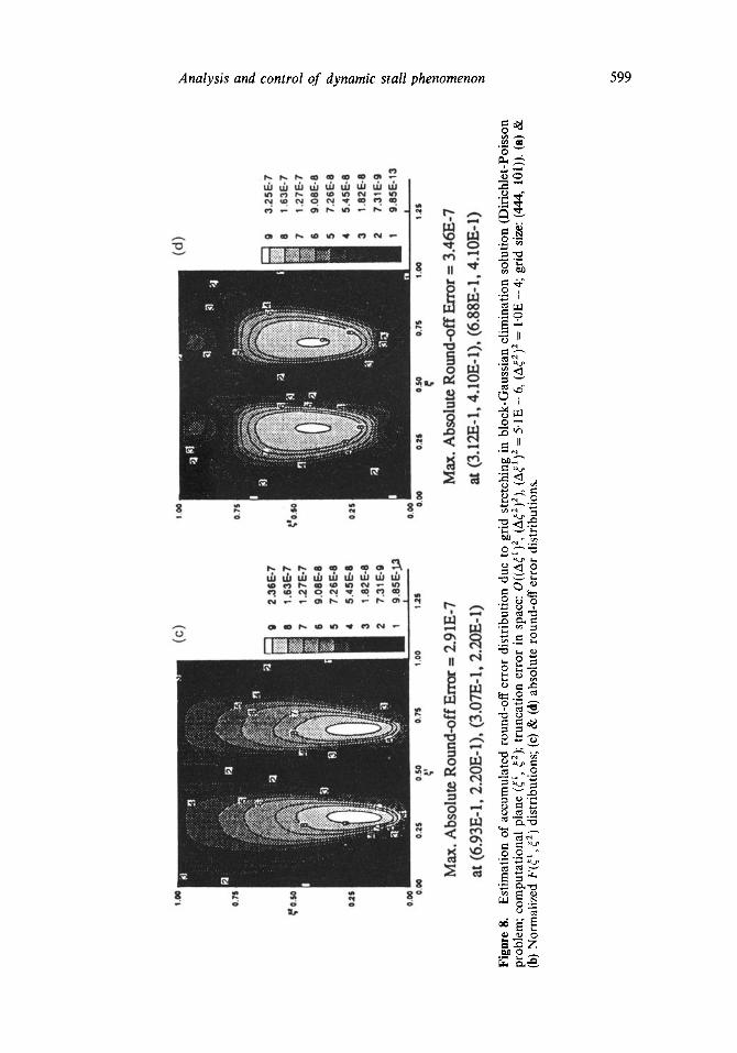
A round-off error study was also performed, and the procedure is as follows. In the Dirichlet-Poisson equation for fro, (14), ¢o is assumed to be known analytically as any one of the two functions prescribed in figure 8. With this function, the source term involving o h is computed numerically using a finite-difference stencil, with extended precision. The computed values of~ol are used to solve the stream function equation, (14), and the numerically computed values of fit ° are compared with the corresponding known analytical values. The diff~.rence in the two solutions represents the round-off error on the present (444 x 101) grid. Figure 8 dearly shows that the maximum error never exceeds 10 -7 for a solution field which lies between 0 and 1. The error also does not exceed the maximum truncation error of O(10-4). In addition, the metric coefficients used in the calculations are shown in figure 9; these are well behaved as expected.
5.2b Grid-refinement study: The grid distribution for all of the three grids mentioned earlier, in the proximity of the NACA 0015 airfoil are depicted in figure 10. For the airfoil at zero angle of attack in flow configuration II, the instantaneous vorticity contours near the TE and, subsequently, in the near wake, are presented here. They show that the flow structure consisting of nearly symmetric vortices at the TE prevails for all of the grids at t = 3.5. As t increases to 4-5, the results of the finer grid show that the vortex symmetry is broken, that is the Hopf bifurcation has just occurred forming the asymmetric needle-type vortex structures of opposite sign in the flow field. At still larger time t = 5"5, the flow field results of medium grid show the vortex shedding process is not only lagging behind the fine grid results but is also out of phase with the latter results. The coarser results still continue to show further growth of symmetric vortical structure near the TE. For truly unsteady flow, it is difficult to carry out this grid refinement study, but, in light of the present results the degree to which the differences are observed is clarified.
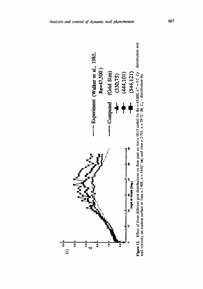
Once the asymptotic state is achieved for the flow field with the airfoil at zero angle of attack, tho constant-rate pitch-up motion with ~i + = 0.2 is initiated. The results in terms of the instantaneous vorticity contours for 15.96° ~< ~ ~ 35"44 ° are delineated in figure 11. The coarse-grid results are quantitatively different. It should also be stated that, compared to the results in figure 10, results for the medium grid do show a departure from the fine-grid results, although qualitatively the two structures are very similar. Thus, the results in figure 11 suggest that the grid be further refined and then see if the changes are smaller than the previous refinement in which grid size was changed from (444 x 101) to (544 x 121). Unfortunately, the results with the (544 x 121) are computationally very costly, with the total cPu time for the fine grid case nearly 5 times higher than for the medium grid using a single processor on the CRAY Y-MP 8/864 at the Ohio Supercomputer Center. Next, the Cp- distribution at the surface as well as the wall vorticity are plotted in figures 12a, b for ct = 14"81 ° and 29"71 °, respectively. For ~ = 14.81 °, where the flow is mostly attached, the surface Cp-distribution for all "three grids is in conformity and it even agrees well with the experimental data of Walker et al (1985). The corresponding wall vorticity shows similar behaviour, as shown in figure 12a; however, there are no experimental data

Cb
O'L
6
"0
1"0
0"8- i.
0"~"
~'O
-
I CO
-
VO
S'O
0"~
0"8 ~
'0
-
'__L~ ,
L _
:"~
.-j~-.
JL lul
,. ...
J~
9"0
~uoz Xa!uguI
£~.'0
OS
'O
SE
O
LI'Z
9ZE
- " "m.IA
I Z~
I90I " "x~IN
O
Olz ~q u
~
08 ol O
I ,~q "~uI
00
"0
m
00
"0
os'o~
SL
'O
00"~.
Ce)

1.0
=.7S
.00
~.2S
ib)
Inc.
by
10
to 8
0 th
en b
y 40
0 M
ax."
151
1.13
M
in."
-34
83.8
3
0.00
I
0.00
0.
2S
O.S
O
O.T
S 1.
00
).8
Infi
nity
Zon
e
).8
).8
1.0
Fig
ure
6.
Eff
ect
of g
rid
stre
tchi
ng o
n fa
r-fi
eld
solu
tio
n-v
ort
icit
y c
onto
urs
in c
ompu
tati
onal
pla
ne.
(Con
stan
t pi
tch-
up m
otio
n; N
AC
A
3015
air
foil
, R
e =
45,0
00;
C-g
rid
(444
, 10
1);
vort
icit
y di
stri
buti
on (A
DI s
olut
ion)
.) (
a) T
ime
= 1.
50,
~t =
20.
54°;
(b)
tim
e =
3-30
, ~t
= 3
6.58
°.
t~
t~ .Ji
.D

(a)
I O
0
0.7S
02
S
0.~
0.0
0
0.2
5
0.50
0
.75
1.
00
0.26
0.20
0.
15
0.10
0.
08
0.05
0.
00
-0.0
6 I
~.2S
• D
iric
hle
t (b
od
y su
rfac
e,
infi
nit
y)
wit
h
sym
me
tric
co
nd
itio
n
(bra
nch
-cu
t)
- P
ois
son
p
rob
lem
fo
r B
GE
so
luti
on
•
c~ =
20
.50
°
Ma
x. l
%°l
:O.2
66
at
(0
.81
7,
0.3
2)
• c~
= 3
6.5
8 ~
'
Ma
x. 1
~°1:
0.35
5 at
(0.6
01
, 0.
41 )
• 0
.0 c,
~<
~ ~<
36
.58
°
0.0
83
~<
Ma
x. I%
°1 ~<
0.3
55
3",
C~
¢h
C~ ?

ib) '" tlilmm
lmll
',~
: ~.~
0,,
ml?
i
# !
~' ,.s
o i/~
.~#e
~
0.25
~
~!
0.00
0.
25
0,50
0.
Ttj
1.00
0.30
0.20
0.
10
0.05
0.
00
-0.0
5 -0
.10
-0.2
0 -0
.35
I 1.2S
',o
,o)
Com
puta
tiona
l Pl
ane
( ~,1
~2)
~2
Infin
it), (
oo) I
In-C
omin
g Fl
ow
( a
= 0 °)
t_ Bo
dySu
rf ac
e
Bran
ch C
ut A
C1,0)
OO
Figu
re 7
. E
ffec
t of
gri
d st
retc
hing
on
far-
fiel
d so
luti
on -
dis
turb
ance
str
eam
fun
ctio
n di
stri
buti
on (
BGE
solu
tion
) in
com
puta
tion
al
plan
e.
Dth
er c
ondi
tion
s in
clud
ing
tim
e an
d c(
val
ues
for
(a)
and
(b)
as i
n fi
gure
6.
e~ Jt ,O
-.O

598 K N Ghia. d Yang, U Ghia and G A Osswatd
0 ~ ~ 0 , . . . . . . . ~ . ~ 0 0 0 0 0 0 0 0 0
2 0 Y
0 ?
II
S ~
v
H,,,,
o o o
° 8 !
i !
It
S "i
,..
,.oo
..
..
.
(d)
,q
8 ..
....
..
: ~ -8
1
D.?S
O
.?S
9 3.
25E
-7
| 8
1.63
E-7
~o
.so
I~'o
.so
7 1.
27E
-7
S 9.
08E
-8
5 7.
26E
-8
o~s
o=s
4 5.
45E
-8
3 1.
82E
-6
2 7.
31E
-9
1 9.
85E
-13
O.O
Q
0.00
I
~!
I .
0.00
0.
2S
0 ,S
O
O.?
S 1.
00
1 25
0.00
0,
~$
0.50
0,
75
1.00
1.
25
Max
. Abs
olut
~ R
ound
-off
Err
or" :
2.9
1E-7
M
ax. A
bsol
ute
Rou
nd-o
ff E
rror
= 3
.46E
-7
at (
6.93
E-1
, 2.
20E
-1),
(3.
07E
-1,
2.20
E-1
) at
(3.
12E
-1,
4.10
E-I
), (
6.88
E-1
, 4.
10E
-l)
Figu
re 8
. E
stim
atio
n of
acc
umul
ated
rou
nd-o
ff e
rror
dis
trib
utio
n du
e to
gri
d st
retc
hing
in
bloc
k-G
auss
ian
elim
inat
ion
solu
tion
(D
iric
hlet
-Poi
sson
pr
oble
m;
com
puta
tion
al p
lane
(~1
, ~2)
; tru
ncat
ion
erro
r in
spa
ce:
O((
A~)
2, (
A¢2
)2),
(A~I
)2 =
5.1
E-
6, (
A~2
) 2=
I'0
E-
4; g
rid
size
: (4
44,
101)
). (a
) &
(b
) Nor
mal
ized
F(~
t, ~
2) d
istr
ibut
ions
; (c
) &
(d)
abs
olut
e ro
und-
off e
rror
dis
trib
utio
ns.

0.75
0.50
¢
0.2S
(a)
600 K N Ghia, J Yang, U Ghia and G A Osswald
at (2.26E-3, 5.0E-3) 3) 3 at (2.66E-1, 9.95E-1) -1)
0.00 0.00
1.00
0.75
0.50
0.25
(b)
0.25 0.50
t
)
1
0.78 1.00 1.25
I at ( 2 .65E-1 , 1.0EO) ) 3 at (1.0E-3, O.OEO)
0.00 0.00 0.25 0.50 0.75 1.00
1 1 1
1.25
Figure 9. Distribution of metric coefficients, for round-off error study (computa- tional plane (~, ~2); grid size: (444, 101)). (a) G11. (b) G22fl.
available for wall vorticity. On the other hand, at ~ = 29'71 °, with massively separated flow regions, the surface Cp-distributions show significant changes, although qualitatively they do conform to the experimental results given by Walker et al (1985). In figure 12b, the wall vorticity on the suction surface does show significant departures, again questioning the grid independence of the results between the medium and fine grid at this level of the grid size. The only satisfactory comparison is that for C L, as shown in this figure. It depicts that the coarse-grid results compare well with the

Analysis and control of dynamic stall phenomenon 601
experimental data of Walker et al (1985). However, the medium- and fine-grid results predict higher CL-distribution in the massively separated flow regime. A careful examination of the experimental set-up reveals that Walker et al (1985) had only 36 surface static pressure taps, as compared to about 207 grid points in the present simulation with (a.AA X 101) grid points. Thus, better resolution in the computational simulation permits determination of each of the individual vortices that evolve and carries with it somewhat higher values for C,-distribution as compared to the corresponding experimental values. Hence, for the finest grid presently used, still larger values of CL are seen in this figure.
5.2c Comparison with available Navier-Stokes results: Simulation results are also obtained for a sinusoidally pitching NACA 0012 airfoil with Re = 5,000, ~ = 10°(1 - cos kt), and reduced frequency based on chord length, k = 1.0. Some experimental data are available for this configuration from Werl6 (1976). Also, Mehta (1977) has provided carefully simulated Navier-Stokes results using the NS equations in terms of (o3, ~k). He has used an O-grid topology and provided detailed results. As seen in figure 13, the streaklines for the present results compare favorably with the experimental data of Werl6 (1976) and show a flow structure representative of unsteady flows. The flow is separated over the entire suction surface. Also shown in this figure are the contours of instantaneous vorticity and the velocity vectors. The better resolution of the present results is clear and these results conform well with those of Mehta (1977). For this sinusoidally pitching airfoil, the instantaneous stream-function contours are compared in figure 14. The results first show one instant for • = 18.59 ° in the upward stroke, which goes up to ~ = 20 °, and then four values of • for the return stroke. For the stream function, which is not very sensitive, the agreement is good. For the same values of ~, comparison is also provided for the instantaneous vorticity contours in figure 15. The qualitative agreement between the two sets of results is very good, although the better resolution of the present results due to the use of a finer grid, made possible by a better and larger computer, is very evident. The complete evolution of the dynamic stall event is vivid, and some of the interactions that take place can be inferred from this figure. Finally, the CL-distribution, as well as the surface pressure coefficients for two values of ~, namely, ~ = 18.57 ° during pitch-up and ~ = 11.11 ° during pitch-down, are shown in figure 16. Also shown in this figure are the results of Sankar & Tassa (1980). In general, CL compares qualitatively with the existing results, but there are significant deviations. For the time being, this completes the verification study; additional verification with experimental data is provided in the next section.
5.3 Influence of initial state on the flow field
For flow configuration II, results are initially obtained to determine the asymptotic state at fixed angle of attack. Since this asymptotic state is not unique, the effect of the initial state of flow will prevail in the final solution. To determine this effect, three different asymptotic states are selected, and correspond to states (b), (c) and (d) on the CL-history curve in figure 17 corresponding to ~ = 0 °. With these states as the starting solutions, three different calculations are made for constant-rate pitch-up motion and the results are compared in figure 17. The lift coefficient distribution, as well as the viscous circulation, for all three cases do conform with one another and do not show strong influence of the initial state. The instantaneous vorticity contours

Gri
d si
ze:
(330
,75)
(a)
Tim
e -
3.5
Max
.; 10
83.9
9 M
in. ;
-108
5.80
(b)
Tim
e =
4.
5 M
ax.;
1081
.38
Min
. ;- 1
083.
20
(c)
Tim
e =
5.5
Max
.; 10
77.1
6 M
in. ;
-108
2.17
(d)
o.
3O
O,
2"S
o. 2
0
O.~
S
O.
bO
O. O
~
0.00
-o,
o~
-o.
:~I
Fim
e =
6.5
Max
.; 10
81.1
3 M
in. ;
-107
2.96
In
c. b
y 4
to 8
0 th
en 4
0
-0.
15 I
-O.
20
-O, 2
~
o.'4
0 O
.$O
O
. BO
O
. 7O
O
.~
O g
O
1.00
I.
tO
I.~O
1.
30
i. eo
iI
(444
,101
) M
ax.;
1072
.88
Min
. ;-1
071.
91
Max
.; 10
69.5
1 M
in. ;
-107
1.30
Max
.; 10
90.8
2 M
in. ;
-11M
5.72
Max
.; 10
85.6
5 M
in. ;
-105
5.44
(544
,121
) M
ax.;
1065
.97
Min
. ;- 1
063.
73
Max
.; 10
50.6
9 M
in.
;-10
75.0
2
Max
.; 1
075.
99
Min
. ;-
1050
.52
Max
.; 10
44.5
2 M
in. ;
- 108
4.11
¢3
6"
C3 6"

o.
~o
o. Q
o
o.
30
~..
,o
o.~
o
o. o
o
-o.
~o
-o.
2O
-o
3ca
o. ~
o
<._.
(e) o.
m
QI
L~
~ee
,eq
-o.
so
~.o
o
o..
so
i.o
G
t so
j"
~ II
JII
e ,,
O~
m
~ II
IJIG
•
e,m
M
u &i
i.~
4.1
I /
I I
I I
I I
4~1
I I
I 4~
I I
I I
I •
i iI
Ii
• I
• r
I e
IQ
11
~ I
e •
• e
~ I
o l
l •
I o
TII
TII
Figu
re
10,
Eff
ect
of,t
hree
di
ffer
ent
grid
dis
trib
utio
ns
on
asym
ptot
ic
flow
sol
utio
n at
~ =
0 °,
for
Re
= 45
,000
, i
+ =
0.2.
(a)
-(d)
V
orti
city
co
ntou
rs
near
"rE
, (e)
tim
e hi
stor
y of
lif
t co
effi
cien
t at
• =
0 °.
g~
g~

Gri
d Si
ze ;
(3
30,7
5)
(444
,101
) (5
44,1
21)
(a)
Max
.; 70
3.42
M
ax.;
1061
.42
Max
.; 82
7.00
M
in. ;
-308
9.45
M
in. ;
-326
2.17
M
in.
;-33
39.1
8
Co)
Max
.; 20
44.2
2 M
in. ;
-413
7.37
M
ax.;
290
5.62
M
in.
;-42
30.1
3 M
ax.;
3397
.65
Min
. ;-
4482
.60
¢3
¢..., ¢3
6'

Cc)
(d)
0.II~
Max.
; 23
52.8
6 Mi
n. ;-4386.53
Max
.; 25
88.8
8 M
in. ;
-420
5.24
M
ax.;
3096
.37
Min
. ;-4
848.
89
Max
.: 15
30.1
0 M
ax.;
1837
.41
Min
. ;-4
429.
03
Max
.; 24
36.8
9 M
in. ;
-386
6.38
.0.~
-0.8
0
Fig
ure
11.
Eff
ect
of th
ree
diff
eren
t gr
id d
istr
ibut
ions
on
flow
pas
t an
NA
CA
001
5 ai
rfoi
l for
Re
= 45
,000
, ~
+ =
0-2
- co
ntou
rs o
f ins
tant
aneo
us
vort
icit
y. T
ime
= 1.
501,
2.1
01,
2.50
1 &
3.2
01,
and
e =
15.9
6 °,
22"
83 °,
27.
41 °
, &
35.
44 °,
res
pect
ivel
y, f
or (
a)-(
d).
g~
t~

606 K N Ghia, J Yang, U Ghia and G A Osswald
I
v
I
o o~ ~ ,
l l l°llJ° ~ IIWM " i "~
. g
! I I
~d0- ~ o °" "
! N
d
c~
I I I I I
o
8.
S.O
(c)
4.(I
3.0
2.0 ~.o
L ~
r
".~...
0 10
2O
3O
4O
SO
eO
A
n~m
d A
ttack
(Oe~
)
0,0
- E
xper
imen
t
Com
pute
d ..&
_
-Q-
(Wal
ker
et a
l.,
Re,
=47,
500
)
(Gri
d Si
ze)
(330
,75)
(4
44,1
01)
(544
,121
)
1985
,
Figu
re 12
. E
ffec
t o
f th
ree
diff
eren
t gr
id d
istr
ibu
tio
ns
on
flo
w p
ast
an N
AC
A 0
015
airf
oil
for
Re
= 45
,000
, a+
= 0
"2.
Cp
-
dis
trib
uti
on
an
d
wal
l vo
rtic
ity
on
su
ctio
n s
urfa
ce a
t ti
me
= 1.
401,
a =
14
.81
° (a
), a
nd
tim
e =
2.70
1, c
t = 2
9.71
° (
b).
Cr.
-
dis
trib
uti
on
(c)
.
t~
t~

608 K N Ghia, J Yang, U Ghia and G A Osswald
(a) (b)
Streak Lines
Vorticity Contours
(c)
Vorticity Contours
Velocity Vectors Velocity Vectors
Figure 13. Comparison of present work (a), with experimental data of Werl6 (1976, ONERA experiment) (b), and numerical results of Mehta (1977) (c), for NACA 0012 airfoil, Re = 5,000, k = 1'0.
are also shown in this figure and, although there is a phase difference in the develop- ment of the wake, the overall influence is minimal.
5.4 Flow structure for configuration lI: Re = 45,000, no suction
For this configuration, Walker et al (1985) have provided flow visualization photo- graphs for six selected values for angle of attack. These photographs very vividly show initially the region of separated flow near LE and TE and, subsequently, the formation of a highly energetic dynamic stall vortex. Streaklines are plotted in figure 18 at ct = 24 °, 27 °, 30 °, 40 ° and 47 ° and they compare well with the flow visualization data. Further, the CL-history, as well as the surface distribution of Cp, are compared with the experimental data in £gures 19a & b. As seen in figure 19a the CL-distribution agrees qualitatively, but shows higher values of CL. It was also pointed out that

Analysis and control of dynamic stall phenomenon 609
a = 18.57 o (a) o~ = 18.50 o (b)
et = 20 .00 o c~ = 19.99 o
o r = 1 7 . 2 5 o ot = 17.47 o
o r= 11.11 o o r= 11.36 °
0t = 4 . 4 5 o Ct = 4.78 o
-______ - - ~
Figure 14. Comparison of numerical results - (a) present, and (b) those of Mehta (1977) - for NACA 0012 airfoil, Re = 5,000, k = 1"0 - instantaneous stream function.
better agreement with experimental data is obtained for the coarse grid simulation using (330 x 75) points. Also shown here is CL-distribution predicted by Visbal & Shang (1989); this, too, agrees better with the experimental data. In the opinion of the present authors, this is again due to their relatively somewhat coarser grid of (203 x 101) points, coupled with their t reatment of the far-field boundary condition. Next, the coe.~cient of surface pressure distribution is compared for two values, ~t = 14.81 o and 29.71 °, in figure 19b. As seen here, the compar ison with the experimental data of Walker et al (1985) is good for ~ = 14.81 °, whereas, for ct = 29.71 °, the two-
610 K N Ghia, J Yang, U Ghia and G A Osswald
c t = 18.57 o (a) ot = 18.50 o (b)
¢z = 2 0 . 0 0 o O~ = 19.99 o
a = 17.25 o tx = 17.47 o
C t = 11.11 o e~= 11 .36 °
t~ = 4.45 o ct = 4 .78 o
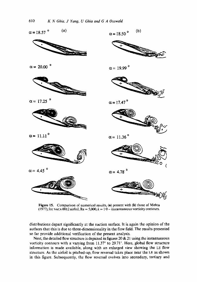
Figure 15. Comparison of numerical results, (a) present with (b) those of Mehta (1977), for NACA 0012 airfoil, Re = 5,000, k = 1"0 - instantaneous vorticity contours.
distributions depart significantly at the suction surface. It is again the opinion of the authors that this is due to three-dimensionality in the flow field. The results presented so far provide additional verification of the present analysis.
Next, the detailed flow structure is depicted in figures 20 & 21 using the instantaneous vorticity contours with ~ varying from 11.37 ° to 29.71 °. Here, global flow structure information is made available, along with an enlarged view showing the LE flOW structure. As the airfoil is pitched-up, flow reversal takes place near the LE as shown in this figure. Subsequently, the flow reversal evolves into secondary, tertiary and

Analysis and control of dynamic stall phenomenon 611
(a ) 2.0
1.S
1.0
O.S
0.0
-0.5
- - M . O ~ . (S~,k~.198o) ~ M - O. (Present)
-1 .c I I ! I 0 S 10 15 20
Angle of At l l¢~ (Dell.)
(b)
~.o (i)
I.o \ X N ~ ~
I~! .0
. . . . " * " ' gIP - I .0
- | . 0 I I I I ¢.w ~ s o.Ts 1.0o 0,H XJC
4.0
,.o ( i i )
2.0
, / \
0.00 02S 0 SO 0,7S 1.00 WC
Figure 16. Compar ison with numerical results of Mchta (1977) and Sankar & Tassa (1980) for NACA 0012 airfoil; Re = 5,000, k = 1-0. (a) C,. vs. ~. (b) C p - distr ibution for (i) t ime=2-601, a = 18.57 ° (pitch-up) and (ii) t ime=4.601 ,
= 11.11° (pitch-down).

w w i w i , , , ~
0
W
m
It. o
CA.
+++
P m
7, ';. |
PlVMssO V D puv V!~lD ~ '/~uv A f 'v!t/D N )/ Z:I9

(c)
Star
t to
pit
ch-u
p at
(1)
) M
ax.
: 63
7.55
Min
. :
-209
7.82
CL
: 0
.980
~tar
t to
pit
ch-u
p at
(c)
M
ax.
: 54
8.50
Min
. :
-208
326
CL
:0.
990
Star
t to
pit
ch-u
p at
(d)
M
ax.
: 49
8.01
Min
. :
-216
6.54
CL
: 1
,106
(D)
I --d
r--
St~
to
j~ch
-up
at (
b)
,.~
(c
)
L~8.O ~ -OA I
.e.l
I
I I
I Lt
) Z
A
6.@
?
A
I0.0
d
,~ac
l (o
eg.)
Figu
re 1
7.
Effe
ct o
f th
ree
diff
eren
t in
itial
st
ates
on
flow
pas
t an
NA
CA
00
15 a
irfo
il; R
e =
45,0
00,
~+ =
0"2
. (A
) T
ime
hist
ory
of l
ift c
oeff
icie
nt
at
~t =
0°;
(1
3) c
ompa
riso
n of
lif
t co
effi
cien
ts,
(C)
inst
anta
neou
s vo
rtic
ity
cont
ours
at
~t =
10-
23°;
and
(D
) ca
lcul
ated
uns
tead
y ci
rcul
atio
n.
g~
t,o
t~
g~

614
(i)
K N Ghia, J Yany, U Ghia and G A Osswald
(a ) (b)
(ii)
(iii)
(iv)
(v)
- -----Y?7:-S~_-
-. '.: .,-Lk; " " ~ ~ - ~ - ~ ; ~ '
~ : - ~ . ~ ~ .-'~,'.._~-n:.~
~/"" " : ? --~), ~.. \ , "Z '~ -~ - ~ .~ / ~ -
i . - . . ; . ~ . . , . ~ . ~ - ~ ,',~ :~-.,_.~1 I I . - - - ~ . ~ , , .~ , ~ . ,~ : . . . . . ~ . ;-;,- ~ . ~ . -__J"'" ~;. ~ . . . . . I , - ,
-.._~ ,<. ~ , i ~ ~ ~ ' , , + ~ . . . . . . , ~ / / / ~ J ' - ~ ~..~4"~ ~,". ~---~. , ( ~ ~
,- L . . .JJ ; 'Z" . " ~ ~ "' X
~ "~'<~-,., -~ --'7- ~!,:_.':. :?.";"::~::. / l ~ f - - ~ -
- d P "
~ ~ f . - " ; . . ~ ~<~
'
OTI IN ]1~1
J. "f~ .
~'t 15, ] I
Y&iS¢ f
~71 15 1 I
Figure 18. C o m p a r i s o n of present wor k (a), with exper imenta l da ta of Walke r et al (1985) (b), for flow past an NACA 0015 airfoil; Re = 45,000, ~ + = 0"2 streaklines. ct = 24 °, 27 °, 36 °, 40 ° and 47 °, respectively, for (i)-(v).

(a) 4.0
3,0
2.0
1.0 %
Analysis and control of dynamic stall phenomenon 6 1 5
0.(I
I I I I I I 0 10 20 30 40 50 M
(b) I,,
I.O 0)
- - - ~ (Walker, a el. . . .-l~ Re,~7,S00, l~lS) m Corn.tee (Pmoat)
4.0
#
V: : : -I .I
8.e
e.O
4.0
2.0
0.0
-l.O
(ii) . / \
J ~ ----- E~Igt ~Iu, M 81.,II~0. _/. ~ R...~7.SOO, ~m)
I I I I 0 2 I 0.$4 0.75 ! .04
x/¢
Figure 19. Comparison with experimental data of Walker et al (1985) for flow past an NACA 0015 airfoil; Re--45,000, ~+ --0-2. (a) C~. vs. ~; (b) C p - distribution for (i) time = 1.401, :t = 14-81 ° and (ii) time = 2-701, ~ = 29-71 °.

0 N
0
0 t%
0
O 2
0
I100
[~ 20
)6g
) 8U ¢
0 80
0 fi0
II 4~I
0 2[
I
0 U
0
0 20
II.~
I
[Lfil
)
il.B
g
~T
'I-II
V~
FII
tIG
IH
[]~
11
3."
I DFG
q 1
2"2~
R
E = ~l[lflll
o TH
IAD
f~T
0 ~i[i
q)- o IF~I-32
0 i~
l 4RII!II~I.
[I~.#
. -
I 1o
i Tl
ff,~
DD
o ~
Gt~
f ,
'.I~
C~
),,I
5 I.,
l~'~
47
l 2
; K
IN
7,~S
0~,
'iS::
t ii
0 50
I)
I)I)
0 ..e
l0 Cm
~ 1.
50
2.00
~.IZ
I_IV
ER
ItIG
TH
FTA
15
.955
D
FG
C L
1.~
12
FII~A
E ~
1 S
01
THTA
DD
=
U.I.
~.~
~ -0
116
1 ¢I]01I"
4011
I 'I
AC
~g
15
M
Jtq;
=
1013
2 411
i'.IN= -3L
~64£
~0 35
2~
~(.
~N
DIT
~
{/~.E
TV'
40(,
T
O B
000
rHE
NB
Y
40
t~
.{{{~
Y~
JIl'~
4~ 4
0.50
o
0o
0.50
1.
00
o ili
I 50
2.
00"
¢3
¢3

(c)
k4A
NE
UV
ER
It4G
T
HE
~A =
18
.21t
6 B
EG
C
t_=
2.07
00
RE
=
45
~.0
T
I~hD
OT
=
0 ~
C D
- 0~
021
~tA
C,~
II)IS
M
A.~
= 10
1500
~
tN=
37
7~.0
1 ,~
4(I
~I
RI~
JND
IE
INC
~Y
40
0 T
O B[L00
THENBY ~
,).~1
030
i~
OAO
3~;I,
,~
l,0
020
,~I.
,00
o.~o
•
- ,l.o
.so
o.oo
&o
,.&
, ,.;
o ~.o
o
(d)
0.130
O.lJO
0,4tl
0.20
0.00
-0.20
6.40
-13.81)
-LLB
O :
i0~5
0 ~q
Et.
~E
RI~
~H
ETA
-
20.5
:~
DE
G
C L
= 2.
4413
R
E =
4~
8~n.
0 T
I~A
DO
T=
0.
2n~
~ 0~
7~1
rIM
E=
13
01
IHTA
DD
=
l).k~
LI
C~S¢
-.0
27£~
i ~
0~
NA
C¢0
015
MA
X=
18
1g.~
7 ki
N=
-4
118.
44
f~O
JND
IE
Ib/£
,~
4.00
3iOBb.O0
ittE
|'~
40
.00
4.~1
1
Fig
ure
20.
Det
ails
of
flow
str
uctu
re f
or N
AC
A 0
015
dirf
oil;
Re
-- 4
5,00
0, ~
+ =
0"2
- in
stan
tane
ous
vort
icit
y co
ntou
rs
for
tim
e =
1.10
1,
1-50
1,
1.70
l &
1.
901,
and
~ =
11
.37
°, 15
.96
°, 18
.25
° &
20
.54
o, r
espe
ctiv
ely,
fo
r (a
)-(d
).
t~

(a)
:b)
,~b~
lF I M
FI
It~G
TH
E I,
~ 27
H:lq
D
~G
~t
~
f~q
o
l N1A
DO
T
ii 7
~
lt~
][
2 H
it
I HT,
~DD
II
~I'A
It-I
) IE
I~
:~"
4L I'I
10
ttllt
llJ
I ~11
)
I B0
I:~lJ
I I;0
i 40
L60
~0
50
I) gl
)
i) 2
/)
U V
U
0 20
o,~-
l}
i),6
fl
ILI]~I
rotH
: 42
"10
14
i,,"
; ,)
?,-i:~ ,,J
~,aC
,EI
P~
RIN
G
TI41
-1~
?~i 2
~
DE
C
C L
: 2
.";~
7 ~
f=
4~fh
'~'ln
IH
TA
DO
T
~ Q
,'~H
I C
'4~
1~
2
~t-.~
.INI)
I~
II~
.I:I
Y
401)
[O
B
0011
]}
tEN
BY
4t
) t.
~ 1~
1.
[I~50
I)
i)O
0.50
i.
i~
I 50
20
D
~h

Figu
re 21
.
~gur
e 20
).
(c)
d:Y
0.80
0.50
04
0
i).20
0,00
-0.2
0
-0.4
0
-0.6
0
-0.8
0 I
0.80
G.8
0
0.4a
0,20
0.00
-0.2
0
-0,4
0
-0.6
0
-0,8
0
M~q
E'L
P~E
HIN
G
TH
ET
A
= L
~fi
0
DE
G
CI_
= 2.
6836
R
E-
4.S
Jb'lf
l.II
Tlf
fAD
OT
=
(I.~
0
~ 0.
8141
TI
kAE =
2
601
THTh
DO
=
O.0
OO
C
K~
-0.Z
~fi
N.A
C~
OlS
I./
a~<
= 26
.q6.
ocJ
I,|N
=
4715
,B0
"~
RE
LI~
DT
E
11
~;~
4(
:=0
TO
B0.
00
TH
EN
BY
~
),00
!ilia,
L 0
50
0.
00
0.50
I .
C~
1 .aO
2,
00
4AI~
',IE:L
D~R
ING
TI'LqA
- 2g.706
DEG
|E = 4~.0
THTADOT-
0.L~
IM~ =
2301
THTADD =
0.~
tCO
ND
TE
IN
C ~
4.
00
TO
B0.
0@
0.50
0.
~0
0.50
1.
00
C L
- 2,
8478
CO
= 12
792
C4~
-0.
~r86
14E
N fi
'Y
~.0
0
' 51~t
°°ij
.-2
1,50
2.
00
Det
ails
of
flow
str
uctu
re f
or N
AC
A 0
015
airf
oil;
a --
-- 22.
83 °,
26.
27 °,
28.
56 °
& 2
9.71
°, r
espe
ctiv
ely,
for
(a)
-(d)
(ot
her
deta
ils a
s in
] g,.
~D

3AS
E
1
L2
me
C~S
E z
j! {0
00
6-0
09
2 ,
Jc)
I ~
! V
(0
7S
7-0
89
4 ~
c)
I T.I
!4
2. t
2.2
2 -1
2.
4 2
-~
Tim
e (t
" LU
c)
! L
+1
(i) ~2
|
[ I
I I
I f
I '
i J
• 12
1.
1 t
I ~
J Z.
1 2.
2 2.
1 2.
4 2~
$
ic)
Ca)
Id)
--
w~
$u
ctlo
fvLr
qecu
ol~
+ C
~S
E 1
•
~ C
.,AS
E 2
I i
, ,
,J IL
l 0-
2 X
/C
0.4
e.l
bJ
=L

(ii) i |
Le
u xJ
C
0.4
o.I
(iii) t|
|
£2
I I
I I
Figu
re 2
2.
Eff
ect
of s
ucti
on/i
njec
tion
fo
r N
AC
A 0
015
airf
oil;
Re
= 45
,000
, ~+
= 0
"2,
v,/
U~
=
0.0
45 (
case
1)
and
0.03
5 (c
ase
2).
(a)
Tim
e hi
stor
y of
con
trol
mod
el f
or s
ucti
on/i
njec
tion
; (b
) ca
lcul
ated
uns
tead
y ci
rcul
atio
n; (
c) v
eloc
ity
vect
ors;
(d)
C,
dist
ribu
tion
. T
ime
= 2"
201,
2.
301
& 2
.401
, an
d ~
= 23
.98 °
, 25
.12 °
& 2
6-27
°, f
or (
i)-(
iii),
resp
ecti
vely
.
g~
~t
O~
I'
,J

II
II
(a)
I m
(i) ii I f~
- '~ (b
) -M
J~
~'dm
'' -2
~ G
~f2
! I
LI
LT
X/C
0,
4 I LI
-I ! -|
m
lii 'I: I~
~| -~
IL
4
W~
S
uc~
or~
ec~h
C.~
SE
2
t~
rJ
o~
X
/C
Li
Lli
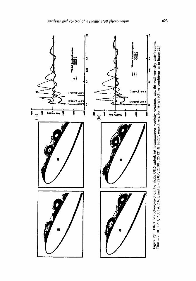
Analysis and control of dynamic stall phenomenon 623
. - ~ . ~ _ , : ~
, ~ I , , 8~ i~!,,,.-.-,! ! ~ I~-.^,.,,! ! ! ~a
e ; e ~ z ,
¢xl

4.0
3.0
.J
O
Co)
2.0
--4-
- C
ASE
t
CA
SE 2
(a) l.O
+I.
0 I
I
m~m
+ o
l A..
= (m
,,O.P
'.°
I 21
.0
I.I
1.2
Wit
hout
S
uc¢i
eNIr
~jec
tion
• -e
--
CA
SE
I
~.
8 O.I
0.4 16
.0
I ,I=
,,,
I 20
,0
24.0
28
.0
Ang
J, v
A
ttac
k (D
eg.)
q~
q~

(c)
(d)
O.I
N
.0.2
S
-0.8
0
LO
07
1
• °
ILO
W'd
ho~
Suc
tion
llni~
tion
--
e-
CA
SE
1
CA
SE
2
W'd
ho~
Sua
iont
l~oc
~im
S.
O
"41
"-
CA
SE
1
CA
SE
2
~.o
I~,.
,,
I ,
I I
2.0
I I
2°'°A
n~e
i* At
tack
(C~.
~ 4"
° n.
o ~6
.o 2°
'°k~e
d ,
~,=
(Oq.
~ 4"
°
Figu
re 2
4.
Effe
ct o
f su
ctio
n/in
ject
ion
for
NA
CA
001
5 ai
rfoi
l. C
ompa
riso
n of
com
pute
d lif
t co
effic
ient
s (a
), dr
ag c
oeff
icie
nts
(b),
mom
ent
coef
ficie
nts
(e)
and
lift/d
rag
rati
os (
d). (
Oth
er c
ondi
tion
s as
in
figur
e 22
.)
¢%
g~
I 24
1.0
O~
Lot

'F (a
)
'r r
~'? +'
~ CA
SE 3
II
/
(0.0
06
-0 0
92
X
/C)
7/
°-'7
, ,
, ,
10
.75
7
O~
I
! 2
0 2.
1 Z
~ 2
"l
2.4
l..ll
Tim
e
(i"
LL
/c)
Z. 04
02
11 I
(b)
/ .-
o--
C
AS
E1
/
._+_
. C
AS
E3
! I
I ,I
I
I I
I I
I IJ
1.
7 I.
I 1.
1 Z
.0
2,1
22
Z
"~
Z.4
2 s
T
im
(t*
Uj¢
)
ii
(c)
(i)
(d)
i ,,
| I
I I
U
U
~G
&
4 L
I
I',J
,=
::=.-

tO
(ii) " o I1
11
liii) III
• o
I I
,,, I
I u
~ XI
c o,
4 LO
Figu
re 2
5.
Eff
ect
of s
ucti
on/i
njec
tion
fo
r N
AC
A
0015
air
foil;
Re
= 45
,000
, a+
= 0
-2,
vs/U
oo =
0"04
5, t
o =
0'05
(ca
se 1
) an
d 0.
15 (
case
3).
(a)
rim
e hi
stor
y of
con
trol
m
odel
; (b
) ca
lcul
ated
un
stea
dy
circ
ulat
ion;
(c
) ve
loci
ty
vect
ors;
an
d (d
) co
effi
cien
ts
of p
ress
ure
dist
ribu
tion
. ri
me
= 2.
201,
2.3
01 &
2.4
01 a
nd c
t = 2
3.98
°, 2
5-12
° &
26-
27 °
for
(i)-
(iii)
, re
spec
tive
ly.
t~ 52

i (a)
U
m
4~
(i) z
~ 1 4
M,
4m
4m,
(ii) -4
m
(b)
--
Wlm
ouc
Suc
~o~
ecll
on
CA
SE
1
C.4+
SG 3
-S~!
7
I I
I 11
,8
IIJ
XiC
11
4 I1.
11
~ +.~j
.j ,+
.*
....
__
---.
...
Wll
l~4
Stx
:llon
t Inj
eclk
m
C.A
SG
I C
,AS
G 3
I I
I !
C,O
+.....
?

I I
]PI !.I !
-|I
,
~
Su
aa
v~
-.
e--
~
E
l ~
G
3L
I I
u u
1~
L
4
! u
I I!
(iv '-[ !. I
U
U
g/C
&
4
Fig
ure
26.
Eff
ect
of s
ucti
on/i
njec
tion
fo
r N
AC
A 0
015
airf
oil;
(a)
in
stan
tane
ous
vort
icit
y co
ntou
rs;
(b)
wal
l vo
rtic
ity
dist
ribu
tion
s.
Tim
e =
2.10
1, 2
"201
, 2.
301
& 2
.401
and
u -
-- 2
2.83
°, 2
3.98
°, 2
5-12
° &
26.
27 °
resp
ecti
vely
for
(i)
-(iv
). (
Oth
er c
ondi
tion
s as
in
figu
re 2
5.)
! I.II
~o
¢3
tO
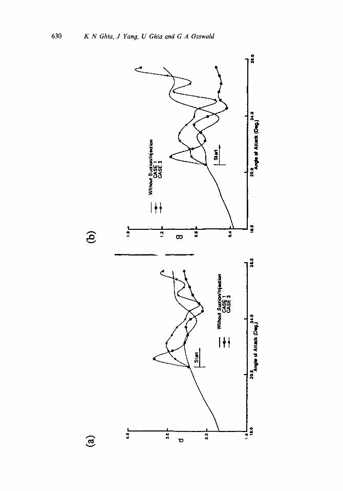
4.0
3.0
2.0
~tl
,~
$.ct
io~l
.ja:t
ion
-e-
CA
SE
1
CA
SE
3
+,o
I I
I ~L
O
20.0
24
.0
2LO
A
~ cl
Att
aci~
(C
~.)
(a)
s,l
1.2
8 011
0.4 II
.0
I I
20,0
24
.0
A~
o+
A..
~,
(C~
)
I 21
.0
c,,,+
.,+

(c)
(d)
0.~
~2
5
.O.S
O
-0.7
S TS
.O
S.O
Wth
o~
Su
~i~'
lnie
dm
n
-4--
C
AS
E 1
C
AS
E 3
W~h
o~ S
uaio
nOIn
iedi
on
S.O
-e
- C
AS
E 1
-*
--
CA
SE
3
Q 4.
0
3.0
I I
ii ,,
! I
I 3.
o I
Figu
re 2
7.
Eff
ect
of s
ucti
on/i
njec
tion
for
NA
CA
001
5 ai
rfoi
l. C
ompa
riso
n of
com
pute
d lif
t co
effi
cien
ts (
a),
drag
coe
ffic
ient
s (b
), m
omen
t co
effi
cien
ts (e
) an
d li
ft/d
rag
rati
os (
d). (
Oth
er c
ondi
tion
s as
in
figu
re 2
5.)

632 K N Ghia. J Yang, U Ghia and G A Osswald
quaternary vortices. The eruption of this secondary vortex structure initiates the formation of the energetic dynamic-stall vortex. K Ghia et al (1992b) have provided further details of this behaviour.
5.5 Flow structure for configuration III: Re = 45,000 with modulated suction injection
In an attempt to control the formation of the dynamic stall vortex, two specific MSI controls were used. These are case 1 with vJU~o = 0.045 and case 2 with vs/U~o = 0.035, as presented in figure 22. The ramp functions used for these two configurations to bring the magnitude of suction velocity to its final magnitude are shown in this figure; these magnitudes are held constant thereafter. Also shown in this figure is the viscous circulation for configuration II as well as for both cases of configuration III. The start of the MSI is also indicated. In addition, the velocity vectors are shown for both cases for three different values, at = 23.98 °, 25.12 ° and 26.27 °. Also shown here are the velocity vectors as well as Cp-distribution on the suction surface for flow without and with MSI. In figure 23, the instantaneous vorticity contours as well as the wall vorticity are shown for configurations II and III. In this figure, results are also plotted for one additional value of0t = 22.83 °. The instantaneous vorticity contours for various values of ct show that the dynamic stall vortex does not develop with MSI activated. Further, the controlled wall vorticity does not show sharp spikes leading to suppres- sion of the formulation of the stall vortex. The results showing the effect of MSI on CL, Co, CM and LID are most significant, since they show directly whether or not the desired control is achieved. Figure 24a shows that there is not much significant change in CL, but, as seen in figure 24b, Co is considerably reduced by MSI for case 1 at higher ~t. Although CM distribution does not show a clear trend in figure 24c, L/D in figure 24d increases rapidly as compared to that for the flow without MSI. Finally, controlled modulated suction/injection is also attempted using configuration III, with a more gradual application of MSI control as shown in figure 25. Compared to case 1, the viscous circulation is sufficiently reduced for this new case 3. As before, the velocity vectors as well as Cp-distribution on the suction surface are also plotted. The corresponding instantaneous vorticity contours and wall vorticity are shown in figure 26. The results for case 3 with its gradually implemented MS! are very similar to those for case 2, as seen from figures 24 and 27. Finally, the effect of gradually applying MSI also shows significant changes as compared to the standard case 1.
6. Conclusion
An unsteady NS analysis is developed using the (03~, ~ , F(t)) formulation. Inclusion of viscous circulation permits accurate treatment of the far-field boundary condition. The implicit ADI-BGE numerical technique provides a uniformly second-order accurate solution, with higher accuracy for the nonlinear convective terms. The grid-refinement study shows that, for this constant-rate pitch-up motion in the regimes where the flow is massively separated, the finest-grid solutions still show more than desired deviation from those of the medium grid used here to obtain all the solutions. Also, since the experimental pressure distribution is measured using a limited number of pressure taps, the coarse-grid CL-distribution agrees well with these results. We discussed the role of unsteady separation in detail earlier (K Ghia et al 1992) which is therefore not described here. Based on the earlier description, a modulated suetion/

Analysis and control of dynamic stall phenomenon 633
injection control strategy was developed and used in this study. The suppression of LE-flow separation provides a very effective means of controlling the formation of the dynamic stall vortex, even with small volumetric suction rate S = -0.00237.
Recently, the present authors have been able to systematically arrive at a control law using a modulated suction/injection strategy; this work has been presented at the AIAA 3rd Shear Flow Control Conference in July 1993 in Orlando, Florida. In this study, although the authors have attempted to analyse the flow using the critical- point theory of Perry & Chong (1987), it is our belief that the usefulness of this theory in identifying organized vortex structures is perhaps more pertinent in conjunction with the (V, p) formulation of the Navier-Stokes equations. In the current (top ~k~, F(t)) formulation, the vorticity is computed directly, and the vortex structures and locations are directly available.
Some of the fundamental research issues have been listed by K Ghia (1992, pp. 157-73) and addressed in a paper by K Ghia et al (1993). These outstanding issues are summarized here for emphasis. The 2-D analysis developed here is accurate and any further discrepancies observed are due to the three-dimensionality effect. An effort should be made to accurately simulate the three-dimensional flow past this 2-D geometry. Effort is also necessary to incorporate an adaptive-grid refinement in this analysis, in order to obtain higher-Re solutions and also resolve the time scale of the eruption of the secondary structure of O(Re-2/11). The three-dimensional analysis should also be coupled with a large-eddy simulation technique in order to obtain higher-Re solutions of greater practical interest.
The authors are sincerely indebted to many of the personnel of the Computational Fluid Dynamics Research Laboratory, University of Cincinnati; in particular, Chad Yoshikawa, Rahul Rathod, Chris Noll, K S Muralirajan, Keith Blodgett, Tom Rohling, and Tae-Seung Yoo have helped in preparing the video animation and in preparation of the manuscript using LATEX.
This research is supported, in part, by AFOSR Grant Nos. 90-0249 and F49620-92- J-0292, and Ohio Supercomputer Center Grant No. PES080.
List of symbols
a
c Co, C_L, CM C~,, c~o c, d ds*
el , e2 P F,,Fo g g~j
radius of airfoil in circle plane; translational acceleration; airfoil chord length; drag, lift, and moment coefficients, respectively; coefficients of pressure and viscous forces, respectively; pressure coefficient; wing span; increment of surface area; Cartesian unit vectors in the physical plane; local covariant base vectors; complex force vector; net forces due to pressure and viscosity, respectively; determinant of the metric tensor; element of covariant metric tensor;

634 K N Ghia, J Yang, U Ghia and G A Osswald
G, G 11, G22fl
1,.]
I
J k LE
LSP
MSI
P P Po
R Re t
t* 1 2 T(~ , ~ , t)
TE
U~ Us
V °, V* f X1X 2
z
Z o~f
~B 6 +
F
Fin q ql,q2
OB v
P E (Din
qJ" q~i." (-t) I
~B
metric coefficients of Dirichlet problem; unit base vector of the inertial Cartesian frame; inertial coordinate subscript; identity tensor; Jacobian determinant; reduced frequency based on chord; leading edge; leading-edge stagnation point; net moment due to pressure and viscosity; modulated suction/injection; unit normal vector to the surface; normal velocity component for MSI; pressure; also, pole locatiorr of cusped trailing edge; complex-potential plane coordinate; complex-potential plane coordinate for zero-lift; apparent position vector; complex circle plane coordinate; Reynolds number; nondimensional time; unit tangential vector to the surface; dimensional time; tangential velocity component for MSI; trailing edge; freestream velocity; constant MSI rate; apparent, translational, inertial, disturbance, and complex velocity vectors, respectively; body-fixed Cartesian coordinates; complex physical plane coordinate; circular cylinder plane coordinate; flow angle of attack; angular acceleration of pitch-up maneuver; non-dimensional pitch rate; viscous circulation at infinity; inviscid circulation; complex q-plane coordinate; q-plane coordinates; angle of pitch-up maneuver; kinematic viscosity of the fluid; complex computational plane coordinate; generalized-coordinates of the non-inertial body-fixed frame; free stream density; summation symbol; inviscid potential function; stream function; disturbance stream function; inertial and inviscid stream functions, respectively; inertial vorticity; angular velocity vector of pitch-up maneuver.

Analysis and control of dynamic stall phenomenon 635
References
Carr L W 1985 Dynamic stall: Progress in analysis and prediction. AIAA paper No. 85-1769 Carr L W (ed.) 1990 Proc. of NASA/AFOSR/ARO Workshop on Physics of Forced Unsteady
Separation (M0ffett Field, CA: NASA Ames Res. Center) Chyu W J, Davis S S, Chang K S 1981 .Calculation of unsteady transonic flow over an airfoil.
AIAA J. 19:684-690 Davis R T 1979 Methods for coordinate generation and potential flow solution based on
Schwarz-Christoffel transformations. AIAA cP 799, pp. 180-194 Douglas J, Gunn J E 1964 A general formulation of alternating direction methods, Part I.
Parabolic and hyperbolic problems. Numer. Math. 6:428-453 Fant D B, Rockwell D (eds) 1992 Proceeding of Workshop on Supermaneuverability: Physics
of unsteady separated flow at high angle-of-attack (Bethlehem, PA: Lehigh University) Gatski T B 1991 Review of incompressible fluid flow computations using the vorticity-velocity
formulation. Appl. Numer. Math. 7:227-239 Ghia K N 1992 Analysis of two-dimensional flow structures of forced unsteady separated flows.
Proceeding of Workshop on Supermaneuverability: Physics of unsteady separated flow at high angle-of-attack (eels) D B Fant, D Rockwell (Bethlehem, PA: Lehigh University)
Ghia K N, Ghia U, Osswald G A 1990 Characterization of dynamic stall phenomenon using two-dimensional unsteady Navier-Stokes equations. Proc. NASA/AFOSR/ARO Workshop on Physics of Forced Unsteady Separation (ed.) L W Cart (Moffett Field, CA: NASA Ames Res. Center); also 1992 NASA CP 3144, pp. 129-147
Ghia K N, Hankey W L, Hodge J K 1977 Study of incompressible Navier-Stokes equations in primitive variables using implicit numerical techniques. AIAA paper No. 77-0648; also AIAA J. 17:298-301
Ghia K N, Yang J, Ghia U, Osswald G A 1992a Analysis of dynamic stall phenomenon through simulation of forced oscillatory flows. Proc. 5th Syrup. on Numerical and Physical Aspects of Aerodynamics, Long Beach, CA
Ghia K N, Yang J, Osswald G A, Ghia U 1991 Study of the dynamic stall mechanism using simulation of two-dimensional Navier-Stokes equations. AIAA paper No. 91-0546; also see - Physics of forced unsteady flow for a NACA 0015 airfoil undergoing constant pitch-up motion. J. Fluid Dyn. Res. (1992) 10:351-369
Ghia K N, Yang J, Osswald G A, Ghia U 1992b Study of the role of unsteady separation in the formation of dynamic stall vortex. AIAA paper No. 92-0196
Ghia K N, Yang J, Osswald G A, Ghia U 1993 Analysis of experimental and computational results for incipient separation and dynamic stall. Invited paper to be presented at 3rd World Conference on Experimental Heat Transfer, Fluid Mechanics and Thermodynamics, November 1-5, 1993, Honolulu, Hawaii
Ghia U, Ghia K N 1987 Navier-Stokes equations for incompressible flow. In Handbook of fluids and fluid machinery (ed.) A Fuchs (New York: McGraw Hill) chap. 3
Gresho P M 1991 Incompressible fluid dynamics: Some fundamental formulation issues. Annu. Rev. Fluid Mech. 23:412-453
Gustafson K, Wyss W (eds) 1990 Proceedings of IMACS 1st International Conference on Computational Physics, University of Colorado at Boulder, Boulder, co, laP. 11-15
Helin H E 1989 The relevance of unsteady aerodynamics for highly maneuverable and agile aircraft. Proc. of 4th Symposium on Numerical and Physical Aspects, Long Beach, CA
Huang Y, Ghia U, Ghia K N 1992 Development of a 3-D unsteady Navier-Stokes analysis for submarine afterbody flows. Aerospace Engineering Report, AFL 92-8-77; University of Cincinnati, Cincinnati, on
Lung J D, Francis M S 1985 Unsteady aerodynamics and dynamic aircraft maneuverability. Proc. AGARD Symposium on Unsteady Aerodynamics- Fundamentals and applications to aircraft dynamics (G6ttingen: AGARD) no. 386, pp. 29.1-29.19
Lerner P 1991 Stall tactics. The X-31 is teaching old dogfighters new tricks. Air Space 6: 29-37
Matida Y, Kuwahara K, Takami H 1975 Numerical study of steady two-dimensional flow past a square cylinder in a channel. J. Phys. Soc. Jpn. 38:1522-1529
McAllister K W, Carr L W 1979 Water tunnel visualizations of dynamic stall. J. Fluids Eng. 101:376-380

636 K N Ghia, J Yang, U Ghia and G A Osswatd
Mehta U B 1977 Dynamic stall of an oscillating airfoil. AGARDCP 227, paper No. 23, pp. 1-32 Osswald G A 1981 Analysis and numerical solutions of unsteady two dimensional Navier-Stokes
equations in primitive and derived variables, Master's thesis, University of Cincinnati, Cincinnati, OH
Osswald G A 1992 Some critical issues associated with the physics of unsteady flows during maneuvers to high angles of attack. Proc. 5th Syrup. on Numerical and Physical Aspects of Aerodynamics, Long Beach, CA, pp. 223-224
Osswald G A, Ghia K N, Ghia U 1987 A direct algorithm for solution of incompressible three-dimensional unsteady Navier-Stokes equations. AI~,A CP 874, pp. 408-421
Osswald G A, Ghia K N, Ghia U 1988 Direct solution methodologies for the unsteady dynamics of an incompressible fluid. Computational mechanics 88 (eds) S N Atluri, G Yagawa (Berlin: Springer-Verlag) vol. 2, pp. 5351-5354
Osswald G A, Ghia K N, Ghia U 1989 Analysis of potential and viscous flows past arbitrary two-dimensional bodies with sharp trailing edges. A1AA CP 895, pp. 668-677
Osswald, G A, Ghia K N, Ghia U t990 Simulation of dynamic stall phenomenon using unsteady Navier-Stokes equations. Proc. of IMACS 1st Int. Conf., Boulder, co, pp. 252-261; also, Comput. Phys. Commun. 65:209-218
Osswald G A, Ghia K N, Ghia U 1992 A direct implicit methodology for the solution of the rapid pitch-up of an airfoil with and without leading edge flow control. Lecture notes in physics (New York: Springer-Verlag) 414:463-467
Perry A E, Chong M S 1987 A description of eddying motions and flow patterns using critical- point concepts. Annu. Rev. Fluid Mech. 19:125-155
Rohling T C 1991 Simulation of chaotic flow past airfoils at high incidence usin 9 the unsteady Navier-Stokes equations, Master's thesis, University of Cincinnati, Cincinnati, OH
Salad K, Roache P J 1990 The influence of sweep on dynamic stall produced by a rapidly pitching wing. AIAA paper 90-0581
Sankar N L, Tassa Y 1980 Reynolds number and compressibility effects on dynamic stall of a NACA 0012 airfoil. AIAA paper No. 80-0010
Speziale C G 1987 On the advantages of vorticity-velocity formulation of the equations of fluid dynamics. J. Comput. Phys. 73:476-480
Visbal M R 1990 On some physical aspects of airfoil dynamic stall. Proc. of Int. Syrup. on Nonsteady Fluid Dynamics (ed.) J A Miller, D P Telionis (New York: ASME) FED-vol. 92
Visbal M R, Shang J S 1989 Investigation of the flow structure around a rapidly pitching airfoil. AIAA J. 27: 1044-1055; also Proc. of AFOSR/FJSRL/DRAM/UC Workshop I1 on Unsteady Separated Flows, FJSRL-TR-88-084, pp 91-108
Walker J D A 1992 Unsteady boundary-layer separation in two-dimensional flows. Proc. 5th Symp. on Numerical and Physical Aspects of Aerodynamics, Long Beach, CA, pp. 131-156
Walker J M, Helin H E, Strickland J H 1985 An experimental investigation of an airfoil undergoing large amplitude pitching motions. AIAA J. 23:1141-1142, also, AIAA paper no. 85-0039
Werl~ H 1976 Visualization hydrodynamique de L'6coulement Autour d'une Pale Oscillante. ONERA Rapport Technique No. 56/1369 AN
Yang J 1992 Study of dynamic stall phenomenon and its control using vorticity, stream function and circulation form of the unsteady Navier-Stokes equations, doctoral dissertation, University of Cincinnati, Cincinnati, OH