ANALYSIS AND COMPUTATION OF A MEAN-FIELD MODEL FOR ...

ANALYSIS AND COMPUTATIONOF A MEAN-FIELD MODEL

FOR SUPERCONDUCTIVITY

Max Gunzburger

Department of Scientific ComputingFlorida State University

Collaborators

Qiang Du

Hyesuk Kwon Lee

Last updated in 1997

1

SUPERCONDUCTING VORTICES

• The fascination of superconductivity centers onits two hallmarks.

Perfect conductivity – the flow of current with-out resistance; in fact, the resistivity of thesuperconducting state is below the detectioncapability of any past or current measuringdevice.

Perfect diagmagnetism – the expulsion of amagnetic field from a sample as it is cooledbelow a critical temperature at which it be-comes superconducting.

• This description of superconductivity applies tometal superconductors in the bulk, i.e., away fromboundaries.

• The situation for other superconductors, includ-ing the recently developed high critical tempera-ture superconductors, is more complicated.

• In particular, mixed states occur in which boththe normal, i.e., nonsuperconducting, and super-conducting phases co-exist.

2

• In this mixed state, the magnetic field can pene-trate the sample in tube-like configurations.

• These tubes of magnetic flux are referred to as(superconducting) vortices.

• Understanding the behavior of the vortices is cru-cial to all applications of superconductivity.

• For example, the motion of these vortices causesOhmic resistance, i.e., a loss of perfect conduc-tivity, so that exploring mechanisms that can pinthe vortices, i.e., prevent them from moving, is ofgreat interest.

3

THE HIERARCHY OF MATHEMATICALMODELS FOR SUPERCONDUCTIVITY

• Superconductivity can be modeled at vastly dif-ferent scales ranging from the atomistic to thatvisible with the naked eye.

• The BCS model of Bardeen, Cooper, and Schrief-fer is universally accepted as a discrete, atomisticmodel for standard superconductors whose mate-rial properties are homogeneous and isotropic.

• The Ginzburg-Landau model of superconductiv-ity is a mezoscale, continuum, phenomenological,steady-state model that resolves phenomena oc-curring in these types of materials on the scale of100 or so A.

• Although this model cannot resolve at the atom-istic scale, it is refined enough that it can re-solve the individual vortex-like structures that oc-cur in the most useful superconductors in partic-ular electromagnetic and thermodynamic config-urations.

4

• In certain restricted circumstances, Gor’kov hasderived the Ginzburg-Landau model from the BCSmodel.

• Time-dependent versions of the Ginzburg-Landaumodel have been developed, as have been ver-sions that account for anisotropies, inhomegeni-eties, and thermal fluctuations.

HOWEVER

• The Ginzburg-Landau model, although being acontinuum model, cannot be used to model anyother than the tiniest of devices.

• The reason for this is that the individual vortex-like structures mentioned above are separated bydistance of the order of 100 or so A, so that cer-tainly a superconducting sample of dimension, say,a millimeter, will contain a huge number of suchstructures.

• It is hopeless to use the Ginzburg-Landau modelas the basis of a numerical simulation of super-conducting phenomena in practical devices.

5

• Thus, at the macroscale, i.e., the scale of devices,one needs to use continuum models that do notattempt to resolve the individual superconductingvortices, but rather that determine an averaged,homogenized quantity such as the density of thesevortices.

• Simple models of this type, e.g., the Bean model,have existed for some time now, and are verymuch in use in the community dedicated to theincorporation of superconductors in the design ofpractical devices.

• However, in many situations, these very simplemodels are known to provide incorrect results sothat better macroscale models would certainly beof use.

6

• Recently, Jonathan Chapman and co-workers havedeveloped mean-field models for the motion ofvortices in the mixed state of a type-II supercon-ductor.

• In these models, the individual vortices are ho-mogenized to give a vortex density, or vorticity.

• The case of vortices in an inviscid fluid was usedas a paradigm problem to derive the models forsuperconductors.

• The models were derived by taking appropriatelimits within the Ginzburg-Landau formalism.

• Our goal is to study one of these models from bothan analytic and computational point of view.

7

A MEAN-FIELD MODELFOR SUPERCONDUCTIVITY

geometry

Ω = bounded domain ∈ RI 2

Γ = boundary of Ω

variables

ω = vortex densityH = magnetic fieldJ = current = ∇H

data

ω0 = initial vortex densityH1 = external applied magnetic fieldJc = critical current

J < Jc ⇒pinning forces are sufficiently strong so that thevortices are not moved by the passage of the cur-rent, and perfect conductivity is retained

J > Jc ⇒the Lorentz force on the vortices due to the cur-rent is sufficiently strong so that the pinning forceis overcome and vortices move

8

The mean-field model (Chapman, et al.)

ω = H − λ2∆H in Ω× (0, T )

ωt −∇ · (m∇H) = 0 in Ω× (0, T )

ω|t=0 = ω0 in Ω

H|Γ = H1 on (0, T )

m ≥ 0 and |∇H| ≤ Jcwith |∇H| < Jc whenever m = 0

• λ ⇒ a length scale, known as the penetrationdepth, which gives and indication of how rapidlythe magnetic field varies in the superconductor

• The initial magnetic field H0 can be determinedfrom the initial vorticity ω0 by solving

H0 − λ2∆H0 = ω0 in ΩH|Γ = H1|t=0

• By appropriately normalizing H and ω by Jc, wecan, without loss of generality, set Jc = 1

9

REGULARIZATION

Function spaces

• Standard Sobolev spaces of real valued functionsof (t,x) ∈ RI + × RI 2

Lp(0, T ;W 1,q0 (Ω))

H1(0, T ;W 1,q0 (Ω))

V =L∞(0, T ;W 1,∞0 (Ω))

• Constrained space

K = φ ∈ V : |∇φ| ≤ 1 a.e., φ|Γ = 0 .

• Inner products(·, ·) = standard L2 inner product on Ω< ·, · >= standard L2 inner product in (0, T )×Ω

• We assume the the boundary data H1 is a con-stant along Γ, but not necessarily in time; we setg = −∂H/∂t

• u = H −H1 and u0 = H0 −H1

• ε = arbitrary positive number

10

Regularized problem

∂uε∂t− λ2∆

∂uε∂t

+1εβ0(uε) = g in Ω× (0, T )

uε = 0 on Γ× (0, T )

uε|t=0 = u0 in Ω

where

β0 : L4(0, T ;W 1,40 (Ω))→ (L4(0, T ;W 1,4

0 (Ω)))′

is defined by

(β0(u), φ) =∫

Ω

(|∇u|2 − 1)+∇u · ∇φdΩ

∀φ ∈ L4(0, T ;W 1,40 (Ω))

and where

(ψ)+ =ψ whenever ψ ≥ 00 otherwise

11

• One can easily verify that β0 is a monotone oper-ator

• Assume that the initial data u0 satisfies |∇u0| ≤ 1

• Note that, in terms of our the original dimensionalvariables, this requires that |∇H0 − ∇H1| ≤ Jcwhich can be easily met by, e.g., choosing |ω0|sufficiently small and H1|t=0 = 0

A weak formulation for the regularized problem

(∂uε∂t

, φ) + λ2(∇∂uε∂t

,∇φ)+1ε

(β0(uε), φ) = (g, φ)

∀φ ∈W 1,40 (Ω)

12

EXISTENCE AND UNIQUENESS RESULTSFOR THE REGULARIZED PROBLEM

A priori estimates

LEMMASuppose g ∈ L1(0, T ;H−1(Ω)) and u0 ∈ H1

0 (Ω),where 0 < T <∞ is a given time.

Then, for t ∈ (0, T ) and for any ε > 0, there existsa constant C that is independent of ε such that

‖uε‖L∞(0,t;W 1,20 (Ω)) ≤ C(‖g‖L1(0,t;H−1(Ω)) +‖u0‖H1(Ω))

‖uε‖2L4(0,t;W 1,40 (Ω)) ≤ C(‖g‖L1(0,t;H−1(Ω)) + ‖u0‖H1(Ω))

LEMMASuppose g ∈ L2(0, T ;H−1(Ω)) and u0 ∈W 1,4

0 (Ω),where 0 < T < ∞ is a given time. Let u0 satisfy|∇u0| < 1.

Then, for any ε > 0, there exists a constant Cthat is independent of ε such that

‖∂uε∂t‖L2(0,t;W 1,2

0 (Ω))≤ C(‖g‖L2(0,t;H−1(Ω))+‖u0‖H1(Ω))

‖uε‖2L∞(0,t;W 1,40 (Ω)) ≤ C(‖g‖L2(0,t;H−1(Ω)) +‖u0‖H1(Ω))

13

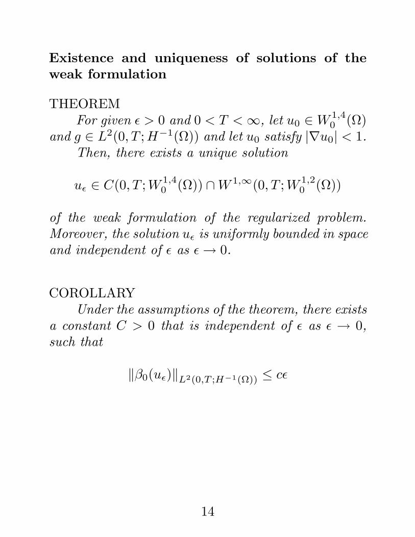
Existence and uniqueness of solutions of theweak formulation

THEOREMFor given ε > 0 and 0 < T <∞, let u0 ∈W 1,4

0 (Ω)and g ∈ L2(0, T ;H−1(Ω)) and let u0 satisfy |∇u0| < 1.

Then, there exists a unique solution

uε ∈ C(0, T ;W 1,40 (Ω)) ∩W 1,∞(0, T ;W 1,2

0 (Ω))

of the weak formulation of the regularized problem.Moreover, the solution uε is uniformly bounded in spaceand independent of ε as ε→ 0.

COROLLARYUnder the assumptions of the theorem, there exists

a constant C > 0 that is independent of ε as ε → 0,such that

‖β0(uε)‖L2(0,T ;H−1(Ω)) ≤ cε

14

PASSING TO THE LIMIT

• We now consider the limit of the sequence uε asε→ 0.

• The lemmas show that the sequence is boundeduniformly in L4(0, T ;W 1,4

0 (Ω))∩H1(0, T ;W 1,20 (Ω))

and in L∞(0, T ;W 1,40 (Ω))∩W 1,∞(0, T ;W 1,2

0 (Ω)).

• Hence, there exists a subsequence of uε thatconverges to u weakly in these spaces. For thelimit function u, we have the following result.

THEOREMLet g ∈ L2(0, T ;H−1(Ω)) and u0 ∈ K.Then, there exists a unique solution of the fol-

lowing variational inequality problem: find u ∈ K ∩H1(0, T ;W 1,2

0 (Ω)) such that u|t=0 = u0 and∫ s

0

[(∂φ

∂t− g, φ− u) + (λ2∇∂φ

∂t,∇φ−∇u)

]dt

≤ 12‖φ(s)− u(s)‖2L2(Ω) +

λ2

2‖∇φ(s)−∇u(s)‖2L2(Ω)

− 12‖φ(0)− u(0)‖2L2(Ω) +

λ2

2‖∇φ(0)−∇u(0)‖2L2(Ω)

∀φ ∈ K ∩H1(0, T ;W 1,20 (Ω))

15

SEMI-DISCRETE FINITEELEMENT APPROXIMATIONS

• We now consider a finite element discretization,with respect to the spatial variables, of the regu-larized problem.

• Suppose Sh ⊂ W 1,40 (Ω) is a finite dimensional

subspace. Specifically, assume Sh is the standardcontinuous piecewise linear finite element space.

• For u0 ∈ K, the initial approximation uh0 is de-fined as the interpolant of u0 in Sh.

• Standard approximation properties yield that

uh0 → u0 in W 1,40 (Ω) as h→ 0

Semi-discretized problem

seek uhε ∈ Sh such that

(∂uhε∂t

, φ) + λ2(∇∂uhε

∂t,∇φ) +

1ε

(β0(uhε ), φ)

= (g, φ) ∀φ ∈ Sh

16

• If we assume that the initial solution is “smooth,”then, we can get uniform estimates for uhε that areindependent of h and ε.

• Hence, as h → 0, the sequence uhε convergesweakly to a limit

u∗ ∈ L4(0, T ;W 1,40 (Ω)) ∩H1(0, T ;W 1,2

0 (Ω))

• The next result is that the limit u∗ is the solutionof the variational inequality problem.

THEOREMLet g ∈ L2(0, T ;H−1(Ω)) and u0 ∈ K. Also, as-

sume that u0 ∈W 2,p(Ω) for some p > 2. Assume thath2−4/p/ε is uniformly bounded and that h/ε→ 0.

Then, as h → 0 and ε → 0, the solution uhεof the semi-discretized weak problem converges weaklyto the solution u of variational inequality problem inL4(0, T ;W 1,4

0 (Ω))∩H1(0, T ;W 1,20 (Ω)).

17

FULLY DISCRETE APPROXIMATIONS

• We again consider a finite element discretizationin the spatial variables.

• There are various ways to implement the timediscretization. For simplicity, let us consider thebackward Euler scheme.

• Given the time step δt, let

gn = g(tn) for tn = nδt, n = 1, 2, . . .

• The initial approximation u0h may be obtained

from∫Ω

(u0hvh + λ2∇u0

h · ∇vh) dΩ

=∫

Ω

(ω0 −H1)vh dΩ ∀ vh ∈ Sh

Discrete variational inequalityFor n = 1, 2, . . ., find unh ∈ K ∩ Sh such that forany φh ∈ K ∩ Sh

(unh−un−1h δtgn , φh − unh)

+ λ2(∇(unh − un−1h ) , ∇φh −∇unh) ≥ 0

18

Lagrange multiplier formulation

• Rather than working with the regularized prob-lem, we consider a saddle point formulation forthe variational inequality using Lagrange multi-pliers.

• Recall that our problem may be written

u− λ2∆u = ω in Ω× (0, T )

ωt −∇ · (m∇u) = g in Ω× (0, T )

ω = ω0 −H1 in Ω at t = 0

u = 0 on Γ× (0, T )

where g = ∂H1/∂t, along with the compatibilityconditions

m ≥ 0 and |∇u| − 1 ≤ 0

m = 0 if |∇u| − 1 < 0

• This may be viewed as a saddle point formulationof the variational inequality where the function mis the Lagrange multiplier.

19

• For the discrete case, let Zh be the set of piecewisenonnegative constants.

• Let

Jn(v) =12

∫Ω

(|v|2 + λ2|∇v|2 − 2v(un−1

h + δtgn))dΩ

andL(v, q) = Jn(v) + (q, |∇v|2 − 1)

• Using the Lagrange multiplier theory, an equiva-lent saddle point formulation is given by:

find (unh, µnh) ∈ Sh × Zh, such that

L(uhn, qh) ≤ L(unh, µnh) ≤ L(vh, µnh)

for any (vh, qh) ∈ Sh × Zh.

20

Uzawa-type iterative solution algorithm

Given (un−1h , µn−1

h ) determine (unh, µnh) by:

1. Set ν(0) = µn−1h . For k = 1, 2, 3, . . . ,K,

a. determine Q(k) ∈ Sh such that

L(Q(k), ν(k−1)) = minQh∈Sh

L(Qh, ν(k−1))

b. set

ν(k) =[ν(k−1) + ρ(|∇Q(k)|2 − 1)

]+in Ω

where ρ is a properly chosen relaxation pa-rameter;

2. Set

unh = Q(K) and µnh = ν(K) in Ω .

For step (1b), one can solve∫Ω

(Q(k)v + (λ2 + δt ν(k−1))∇Q(k) · ∇v

)dΩ

=∫

Ω

((un−1h + δtgn)v + λ2∇un−1

h · ∇v)dΩ ∀ v ∈ Sh

21

Convergence of algorithm

• We now investigate the convergence of the itera-tion as k →∞.

• From the weak formulations, one easily obtainsthat there exists a constant C > 0, independentof k, such that

‖Q(k)‖1 ≤ C and ‖unh‖1 ≤ C

• An inverse inequality then implies that there ex-ists a constant C > 0, independent of k, such that

‖Q(k)‖1,∞ ≤ C and ‖unh‖1,∞ ≤ C

THEOREMThere exists a properly chosen ρ such that

limk→∞

‖Q(k) − unh‖1 = 0

• Unfortunately, in our proof, the constants dependon δt and h.

22

NUMERICAL EXPERIMENTS

• numerical computations were performed using afinite element method based on a triangular meshwith continuous piecewise quadratic polynomialsfor the magnetic field and continuous piecewiselinear polynomials for the Lagrange multiplier.

• Although the theoretical results were proved un-der the assumption that the finite element spacefor the magnetic field is piecewise linear, it wasnecessary to use piecewise quadratic elements inorder to compute the vorticity which involves theterm ∆H.

• Obviously, the theorem is still true with the choiceof piecewise quadratic polynomials.

23

Example 1

• Ω = unit square

• Uniform grid with h = 1/14 and δt = 0.05

• Boundary condition:

H1(t) =t for t ≤ TT for t > T

• Initial vorticity: ω0 = 0

• Penetration depths: λ = 0.1, 0.3, and 0.5

• Corresponding relaxation parameters:ρ = 0.1, 0.8, and 1.0

• Corresponding values of T used:T = 0.2, 0.4, and 0.7

• After the external field H1 became constant, i.e.,for t > T , the magnetic field remained unchangedas well; thus we only report results for t ≤ T .

24

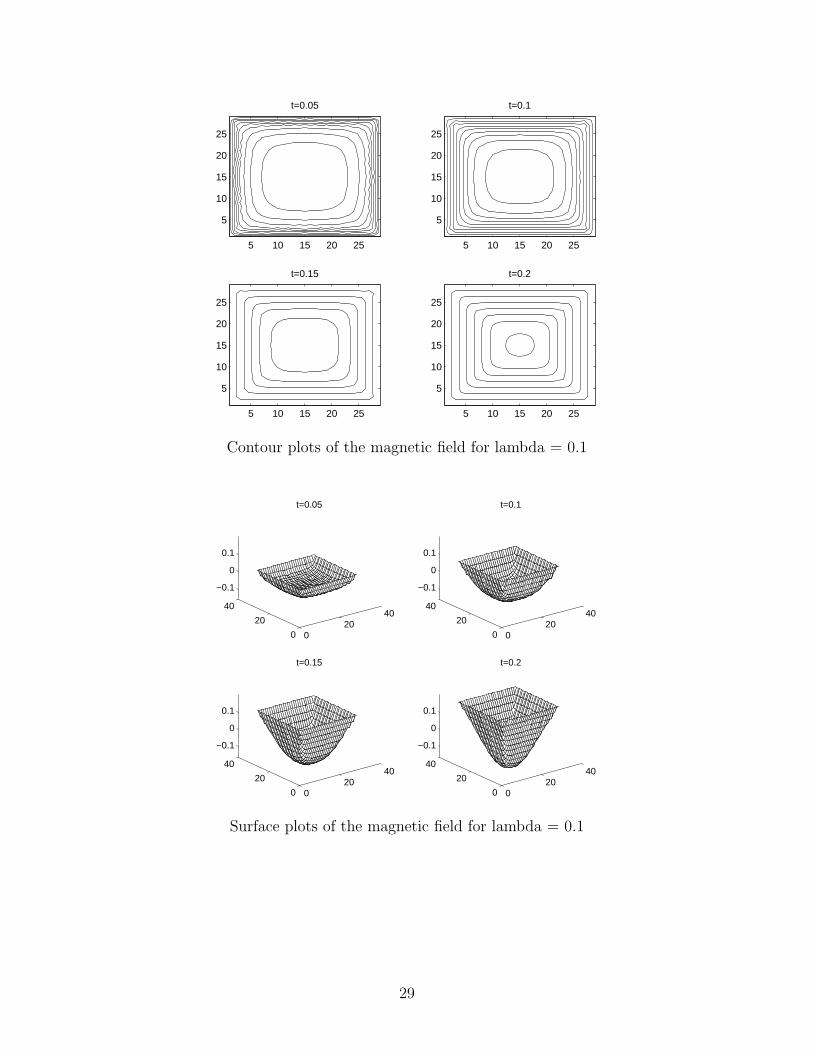
• The surface plots show that the magnetic fieldforms a pyramid as time increases.

• As λ becomes larger, the formation rate gets slow.

• For example, the contour plot for λ = 0.1 at t =0.2 can be compared with the ones for λ = 0.3 att = 0.4 or for λ = 0.5 at t = 0.7.

25

Example 2

• Ω = cross-shaped sample

• Arm length is half of width

• Uniform grid with h = 1/14 and δt = 0.05

• Boundary condition:

H1(t) =

t for t ≤ 0.30.3 for t > 0.3

• Initial vorticity: ω0 = 0

• Penetration depth: λ = 0.1

• Relaxation parameter: ρ = 0.3

• The creation of vorticity occurs first near the reen-trant corners of the cross.

• For later times, in each arm, the magnetic fieldagain forms half of an up-side-down pyramid anda full pyramid in the center of cross.

26

FUTURE WORK

Modeling

develop models that account for– anisotropies– inclusions of normal materials– applied currents– thermal fluctuations

Numerical analysis

more general convergence theory error estimates

Computations

more extensive computational studies

27

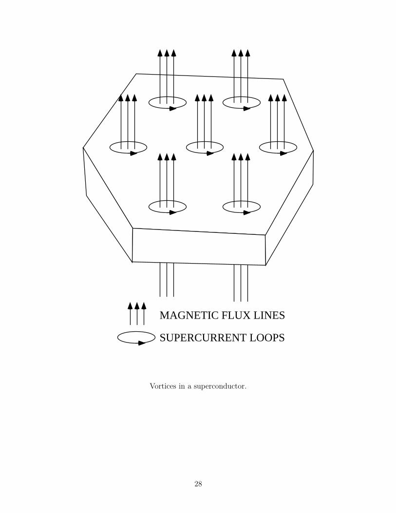
MAGNETIC FLUX LINES

SUPERCURRENT LOOPS

Vortices in a superconductor.

28

5 10 15 20 25

5

10

15

20

25

t=0.05

5 10 15 20 25

5

10

15

20

25

t=0.1

5 10 15 20 25

5

10

15

20

25

t=0.15

5 10 15 20 25

5

10

15

20

25

t=0.2

Contour plots of the magnetic field for lambda = 0.1

020

40

0

20

40

−0.1

0

0.1

t=0.05

020

40

0

20

40

−0.1

0

0.1

t=0.1

020

40

0

20

40

−0.1

0

0.1

t=0.15

020

40

0

20

40

−0.1

0

0.1

t=0.2

Surface plots of the magnetic field for lambda = 0.1

29

5 10 15 20 25

5

10

15

20

25

t=0.05

5 10 15 20 25

5

10

15

20

25

t=0.1

5 10 15 20 25

5

10

15

20

25

t=0.15

5 10 15 20 25

5

10

15

20

25

t=0.2

5 10 15 20 25

5

10

15

20

25

t=0.3

5 10 15 20 25

5

10

15

20

25

t=0.4


30

020

40

0

20

400

0.2

0.4

t=0.05

020

40

0

20

400

0.2

0.4

t=0.1

020

40

0

20

400

0.2

0.4

t=0.15

020

40

0

20

400

0.2

0.4

t=0.2

020

40

0

20

400

0.2

0.4

t=0.3

020

40

0

20

400

0.2

0.4

t=0.4


31

5 10 15 20 25

5

10

15

20

25

t=0.1

5 10 15 20 25

5

10

15

20

25

t=0.2

5 10 15 20 25

5

10

15

20

25

t=0.3

5 10 15 20 25

5

10

15

20

25

t=0.4

5 10 15 20 25

5

10

15

20

25

t=0.5

5 10 15 20 25

5

10

15

20

25

t=0.7


32

020

40

0

20

400

0.2

0.4

0.6

t=0.1

020

40

0

20

400

0.2

0.4

0.6

t=0.2

020

40

0

20

400

0.2

0.4

0.6

t=0.3

020

40

0

20

400

0.2

0.4

0.6

t=0.4

020

40

0

20

400

0.2

0.4

0.6

t=0.5

020

40

0

20

400

0.2

0.4

0.6

t=0.7


33

2 4 6 8 10 12

2

4

6

8

10

12

t=0.05

2 4 6 8 10 12

2

4

6

8

10

12

t=0.1

2 4 6 8 10 12

2

4

6

8

10

12

t=0.15

2 4 6 8 10 12

2

4

6

8

10

12

t=0.2

Contour plots of the vorticity for lambda = 0.1

34

2 4 6 8 10 12

2

4

6

8

10

12

14t=0.05

2 4 6 8 10 12

2

4

6

8

10

12

14t=0.1

2 4 6 8 10 12

2

4

6

8

10

12

14t=0.15

2 4 6 8 10 12

2

4

6

8

10

12

14t=0.2

2 4 6 8 10 12

2

4

6

8

10

12

14t=0.3

2 4 6 8 10 12

2

4

6

8

10

12

14t=0.4


35

2 4 6 8 10 12

2

4

6

8

10

12

14t=0.1

2 4 6 8 10 12

2

4

6

8

10

12

14t=0.2

2 4 6 8 10 12

2

4

6

8

10

12

14t=0.3

2 4 6 8 10 12

2

4

6

8

10

12

14t=0.4

2 4 6 8 10 12

2

4

6

8

10

12

14t=0.5

2 4 6 8 10 12

2

4

6

8

10

12

14t=0.7


36

0 0.5 10

0.2

0.4

0.6

0.8

1t=0.05

0 0.5 10

0.2

0.4

0.6

0.8

1t=0.1

0 0.5 10

0.2

0.4

0.6

0.8

1t=0.15

0 0.5 10

0.2

0.4

0.6

0.8

1t=0.2

0 0.5 10

0.2

0.4

0.6

0.8

1t=0.25

0 0.5 10

0.2

0.4

0.6

0.8

1t=0.3


37

5 10 15

2

4

6

8

10

12

14

t=0.05

5 10 15

2

4

6

8

10

12

14

t=0.1

5 10 15

2

4

6

8

10

12

14

t=0.15

5 10 15

2

4

6

8

10

12

14

t=0.2

5 10 15

2

4

6

8

10

12

14

t=0.25

5 10 15

2

4

6

8

10

12

14

t=0.3


38

ANALYSIS AND COMPUTATION OF A MEAN-FIELD MODEL FOR ...

Documents

Transcript of ANALYSIS AND COMPUTATION OF A MEAN-FIELD MODEL FOR ...