Analysis –Basics of Chapter 1’ Calculus Vector...
33
1 : : : : Chapter 1’ Vector Calculus http://ctaps.yu.edu.jo/physics/Courses/Phys201/Chapter1P Analysis – Basics of Calculus © Dr. Nidal M. Ershaidat Phys. 201 Chapter 1': Vector Analysis 3 Derivative The infinitesimal rate of change in a function with respect to one of its parameters. Derivative !" #$%& ! !" #$%& ! !" #$%& ! !" #$%& ! . . . . The derivative is one of the key concepts in calculus. © Dr. Nidal M. Ershaidat Phys. 201 Chapter 1': Vector Analysis 4 Integral: A mathematical object that can be interpreted as an area or a generalization of area. Integrals and derivatives are the fundamental objects of calculus. Integral
Transcript of Analysis –Basics of Chapter 1’ Calculus Vector...
1
: : : :
Chapter 1’
Vector Calculushttp://ctaps.yu.edu.jo/physics/Courses/Phys201/Chapter1P
Analysis – Basics of
Calculus
© Dr. Nidal M. Ershaidat Phys. 201 Chapter 1': Vector Analysis
3
Derivative
The infinitesimal rate of change in a
function with respect to one of its
parameters.
Derivative
!" #$%& ! !" #$%& ! !" #$%& ! !" #$%& ! . . . .
The derivative is one of the key
concepts in calculus.
© Dr. Nidal M. Ershaidat Phys. 201 Chapter 1': Vector Analysis
4
Integral:
A mathematical object that can be
interpreted as an area or a
generalization of area. Integrals and
derivatives are the fundamental objects
of calculus.
Integral

2
© Dr. Nidal M. Ershaidat Phys. 201 Chapter 1': Vector Analysis
5
Limits
A limit is the value a function
approaches as the variable approaches
some point.
If the function is not continuous, the
limit could be different from the value
of the function at that point.
Differentiation of
Vectors
© Dr. Nidal M. Ershaidat Phys. 201 Chapter 1': Vector Analysis
7
The derivative of a (real) scalar function φφφφ is
defined as follows:
This definition means that this operation is a
local one, i.e. it’s only defined at a given point
in space (x here).
Derivative of a Real Function
( ) ( )x
xxx
x x ∆φ−∆+φ
=φ
→∆ 0lim
d
d
Actually the derivative at some point x is
nothing else but the slope of the tangent to the
function at that particular point
© Dr. Nidal M. Ershaidat Phys. 201 Chapter 1': Vector Analysis
8
Geometrical Representation of a Derivative
The derivative at x is the slope of the tangent
to the function at x. (And we know how to
compute the slope of a straight line!)
(x,φφφφ(x))
x
φφφφ
x
3
© Dr. Nidal M. Ershaidat Phys. 201 Chapter 1': Vector Analysis
9
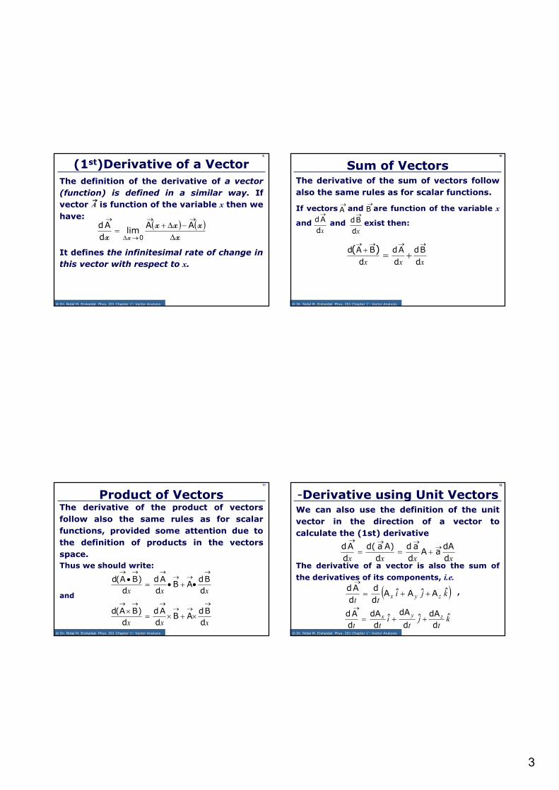
The definition of the derivative of a vector
(function) is defined in a similar way. If
vector is function of the variable x then we
have:
(1st)Derivative of a Vector
→→→→A
( ) ( )x
xxx
x x ∆−∆+
=
→→
→∆
→AA
limd
Ad
0
It defines the infinitesimal rate of change in
this vector with respect to x.
© Dr. Nidal M. Ershaidat Phys. 201 Chapter 1': Vector Analysis
10
The derivative of the sum of vectors follow
also the same rules as for scalar functions.
Sum of Vectors
xxx d
Bd
d
Ad
d
BAd )(→→→→
+=+
If vectors and are function of the variable x
and and exist then: xd
Bd→
→B
xd
Ad→
→A
© Dr. Nidal M. Ershaidat Phys. 201 Chapter 1': Vector Analysis
11
Product of VectorsThe derivative of the product of vectors
follow also the same rules as for scalar
functions, provided some attention due to
the definition of products in the vectors
space.
Thus we should write:
xxx d
BdAB
d
Ad
d
)BA(d→
→→→→→
•+•=•
and
xxx d
BdAB
d
Ad
d
)BA(d→
→→→→→
×+×=×
© Dr. Nidal M. Ershaidat Phys. 201 Chapter 1': Vector Analysis
12
The derivative of a vector is also the sum of
the derivatives of its components, i.e.
We can also use the definition of the unit
vector in the direction of a vector to
calculate the (1st) derivative
-Derivative using Unit Vectors
xxxx d
dAaA
d
ad
d
A)ad(
d
Ad →→→→
+==
,( )kjitt
zyxˆAˆAˆA
d
d
d
Ad++=
→
kt
jt
itt
zyx ˆd
dAˆ
d
dAˆ
d
dA
d
Ad++=
→
4
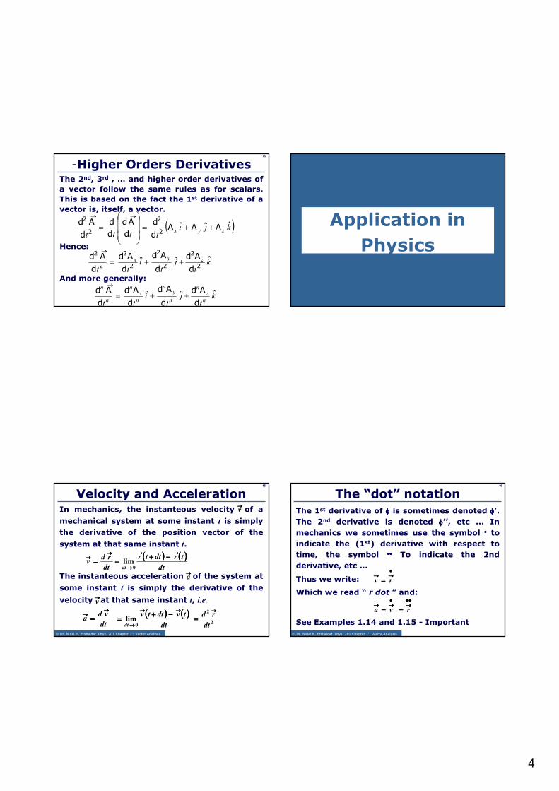
13
The 2nd, 3rd , … and higher order derivatives of
a vector follow the same rules as for scalars.
This is based on the fact the 1st derivative of a
vector is, itself, a vector.
-Higher Orders Derivatives
Hence:
kt
jt
itt
zyx ˆd
Adˆ
d
Adˆ
d
Ad
d
Ad2
2
2
2
2
2
2
2
++=→
( )kjitttt
zyxˆAˆAˆA
d
d
d
Ad
d
d
d
Ad2
2
2
2
++=
=
→→
And more generally:
kt
jt
itt n
zn
n
yn
nx
n
n
n
ˆd
Adˆ
d
Adˆ
d
Ad
d
Ad++=
→
Application in
Physics
© Dr. Nidal M. Ershaidat Phys. 201 Chapter 1': Vector Analysis
15
(((( )))) (((( ))))dt
tvdttv
dt
→→→→→→→→
→→→→
−−−−++++====
0lim
In mechanics, the instanteous velocity of a
mechanical system at some instant t is simply
the derivative of the position vector of the
system at that same instant t.
Velocity and Acceleration
dt
rdv
→→→→→→→→
====(((( )))) (((( ))))
dt
trdttr
dt
→→→→→→→→
→→→→
−−−−++++====
0lim
dt
vda
→→→→→→→→
====2
2
dt
rd→→→→
====
→→→→v
The instanteous acceleration of the system at
some instant t is simply the derivative of the
velocity at that same instant t, i.e.
→→→→a
→→→→v
© Dr. Nidal M. Ershaidat Phys. 201 Chapter 1': Vector Analysis
16
The 1st derivative of φφφφ is sometimes denoted φφφφ’.
The 2nd derivative is denoted φφφφ’’, etc ... In
mechanics we sometimes use the symbol •••• to
indicate the (1st) derivative with respect to
time, the symbol •••••••• To indicate the 2nd
derivative, etc …
The “dot” notation
Thus we write:
••••→→→→→→→→
==== rv
Which we read “ r dot ” and:••••→→→→→→→→
==== va
••••••••→→→→
==== r
See Examples 1.14 and 1.15 - Important

5
17
0====••••====••••====→→→→→→→→→→→→
→→→→
vdvmvddt
rdmdW
We can rewrite the previous expression as follows:
A central force , i.e. it is perpendicular to the
velocity , is exerted on an object of mass m. The
trajectory of the body is circular in a plane
containing both vectors.
Example: Circular Motion
Proof:
→v
0====••••====••••====→→→→
→→→→→→→→→→→→
rddt
vdmrdFdW
→→→→F
Since is perpendicular to the displacement the
work done by the force on the body is zero.
→→→→F
→→→→rd
© Dr. Nidal M. Ershaidat Phys. 201 Chapter 1': Vector Analysis
18
0=•⇒→→vdv
Circular Motion
02)(2
====••••====••••++++••••====••••====→→→→→→→→→→→→→→→→→→→→→→→→→→→→→→→→→→→→vdvvdvvvdvvdvd
This means that the magnitude of the velocity
is constant. The change caused by the force
concerns only the direction of the vector .
The locus of where it keeps its magnitude
constant and changes only its direction is a
circle of radius R given by:
→v
→v
R
vmF
2
====
→→→→Gradient ∇∇∇∇∇∇∇∇
© Dr. Nidal M. Ershaidat Phys. 201 Chapter 1': Vector Analysis
20
The Gradient Operator→→→→∇∇∇∇
Thus dφφφφ appears as “a scalar product” of
two vectors: by (dx1,dx2,dx3).
∂
φ∂∂
φ∂∂
φ∂
321,,xxx
kx
jx
ix
ˆˆˆ
321 ∂∂∂∂∂∂∂∂++++
∂∂∂∂∂∂∂∂++++
∂∂∂∂∂∂∂∂====∇∇∇∇
→→→→
φ∇=∂
φ∂+
∂φ∂
+∂
φ∂ →k
xj
xi
xˆˆˆ
321
by the scalar function φφφφ, i.e.
In the same logic, the vector can
be considered as the multiplication of a
vector denoted
∂
φ∂∂
φ∂∂
φ∂
321,,xxx
→∇
6
© Dr. Nidal M. Ershaidat Phys. 201 Chapter 1': Vector Analysis
21
The vector, symbol nabla or del
The Gradient (del) Operator→→→→∇∇∇∇
kx
jx
ix
ˆˆˆ
321 ∂∂∂∂∂∂∂∂++++
∂∂∂∂∂∂∂∂++++
∂∂∂∂∂∂∂∂====∇∇∇∇
→→→→
ix∂∂ is a differential change in the direction xi.
is called “gradient”.
kx
jx
ix
ˆˆˆ
321 ∂∂∂∂φφφφ∂∂∂∂++++
∂∂∂∂φφφφ∂∂∂∂++++
∂∂∂∂φφφφ∂∂∂∂====φφφφ∇∇∇∇
→→→→
For a scalar function φφφφ we write (read del φφφφ)φ∇→
G
© Dr. Nidal M. Ershaidat Phys. 201 Chapter 1': Vector Analysis
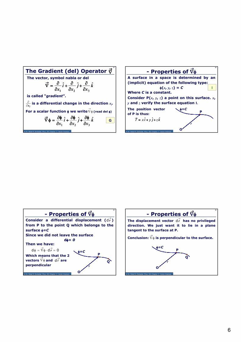
22
φφφφ=CThe position vector
of P is thus:
A surface in a space is determined by an
(implicit) equation of the following type:
- Properties of ∇φ∇φ∇φ∇φ
φφφφ(x, y, z) = C
Where C is a constant.
Consider P(x, y, z) a point on this surface. x,
y and z verify the surface equation I.
I
r
O
P
kzjyixr ˆˆˆ ++++++++====→→→→
→→→→
© Dr. Nidal M. Ershaidat Phys. 201 Chapter 1': Vector Analysis
23
Consider a differential displacement ( )
from P to the point Q which belongs to the
surface φφφφ=C
- Properties of ∇φ∇φ∇φ∇φ→→→→
O
r
P
Q
φφφφ=C
Since we did not leave the surface
0dd =⋅φ∇=φ→→r
→rd
dφφφφ= 0Then we have:
Which means that the 2
vectors and are
perpendicular
→rdφ∇
→
© Dr. Nidal M. Ershaidat Phys. 201 Chapter 1': Vector Analysis
24
The displacement vector has no privileged
direction. We just want it to lie in a plane
tangent to the surface at P.
- Properties of ∇φ∇φ∇φ∇φ→→→→
O
r
P
Q
φφφφ=C
→rd
Conclusion: is perpendicular to the surface.φ∇→
7
© Dr. Nidal M. Ershaidat Phys. 201 Chapter 1': Vector Analysis
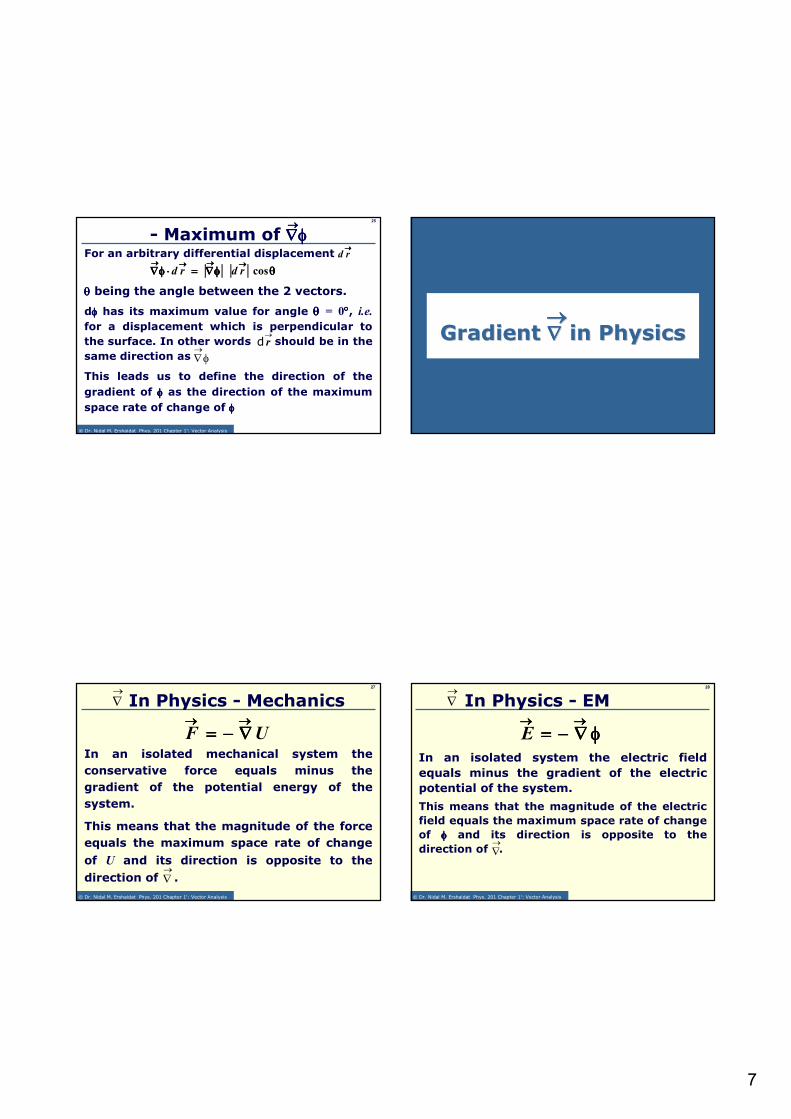
25
- Maximum of ∇φ∇φ∇φ∇φ→→→→
This leads us to define the direction of the
gradient of φφφφ as the direction of the maximum
space rate of change of φφφφ
For an arbitrary differential displacement→→→→rd
θθθθφφφφ∇∇∇∇====⋅⋅⋅⋅φφφφ∇∇∇∇→→→→→→→→→→→→→→→→
cos|||| rdrd
θθθθ being the angle between the 2 vectors.
dφφφφ has its maximum value for angle θθθθ = 0°°°°, i.e.for a displacement which is perpendicular to
the surface. In other words should be in the
same direction as φ∇→
→rd
→→→→→→→→Gradient Gradient ∇∇∇∇∇∇∇∇ in Physicsin Physics
© Dr. Nidal M. Ershaidat Phys. 201 Chapter 1': Vector Analysis
27
In Physics - Mechanics
UF→→→→→→→→∇∇∇∇−−−−====
This means that the magnitude of the force
equals the maximum space rate of change
of U and its direction is opposite to the
direction of .→∇
In an isolated mechanical system the
conservative force equals minus the
gradient of the potential energy of the
system.
→∇
© Dr. Nidal M. Ershaidat Phys. 201 Chapter 1': Vector Analysis
28
In Physics - EM→∇
φφφφ∇∇∇∇−−−−====→→→→→→→→
E
This means that the magnitude of the electric
field equals the maximum space rate of change
of φφφφ and its direction is opposite to the
direction of .→∇
In an isolated system the electric field
equals minus the gradient of the electric
potential of the system.
8
© Dr. Nidal M. Ershaidat Phys. 201 Chapter 1': Vector Analysis
29
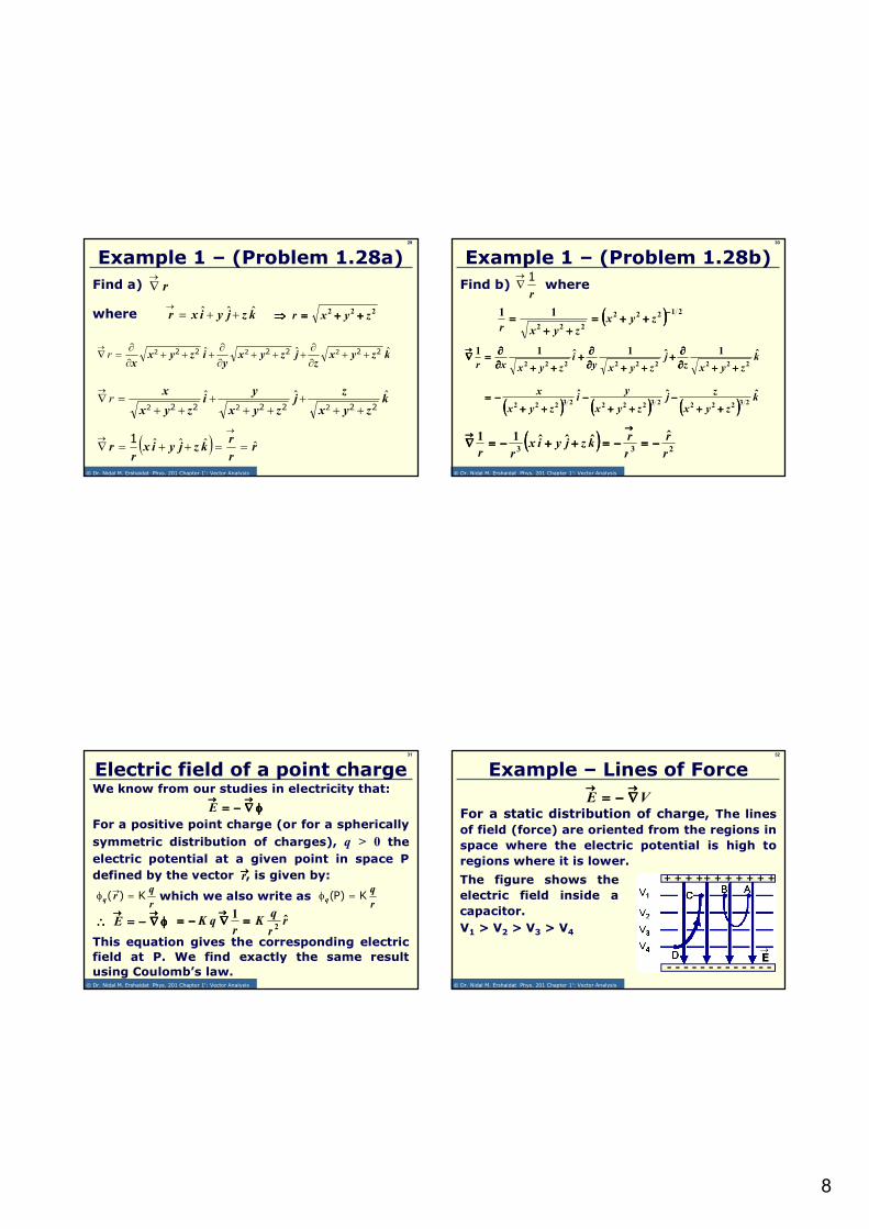
kzjyixr ˆˆˆ ++=→
Find a)
Example 1 – (Problem 1.28a)
r→∇
kzyx
zj
zyx
yi
zyx
x ˆˆˆ
222222 222 +++
+++
++=∇
→r
kzyxz
jzyxy
izyxx
ˆˆˆ 222222 222 ++∂∂
+++∂∂
+++∂∂
=∇→r
( ) rr
rkzjyix
rr ˆˆˆˆ ==++=∇
→→ 1
222zyxr ++++++++====⇒⇒⇒⇒where
© Dr. Nidal M. Ershaidat Phys. 201 Chapter 1': Vector Analysis
30
Find b) where
Example 1 – (Problem 1.28b)
r
1→∇
(((( )))) 21222
222
11 −−−−++++++++====
++++++++==== zyx
zyxr
(((( )))) (((( )))) (((( ))))k
zyx
zj
zyx
yi
zyx
x ˆˆˆ232222322223222 ++++++++
−−−−++++++++
−−−−++++++++
−−−−====
kzyxz
jzyxy
izyxxr
ˆ1ˆ1ˆ11222222222 ++++++++∂∂∂∂
∂∂∂∂++++++++++++∂∂∂∂
∂∂∂∂++++++++++++∂∂∂∂
∂∂∂∂====∇∇∇∇→→→→
(((( ))))233
ˆˆˆˆ11
r
r
r
rkzjyix
rr−−−−====−−−−====++++++++−−−−====∇∇∇∇
→→→→→→→→
© Dr. Nidal M. Ershaidat Phys. 201 Chapter 1': Vector Analysis
31
We know from our studies in electricity that:
This equation gives the corresponding electric
field at P. We find exactly the same result
using Coulomb’s law.
Electric field of a point charge
r
qrq K)( =φ →
For a positive point charge (or for a spherically
symmetric distribution of charges), q > 0 the
electric potential at a given point in space P
defined by the vector , is given by:→→→→r
φφφφ∇∇∇∇−−−−====→→→→→→→→
E
φφφφ∇∇∇∇−−−−====∴∴∴∴→→→→→→→→
E rr
qK
rqK ˆ
12
====∇∇∇∇−−−−====→→→→
r
qq K)P( =φwhich we also write as
© Dr. Nidal M. Ershaidat Phys. 201 Chapter 1': Vector Analysis
32
→E
Example – Lines of Force
VE→→→→→→→→∇∇∇∇−−−−====
For a static distribution of charge, The lines
of field (force) are oriented from the regions in
space where the electric potential is high to
regions where it is lower.
The figure shows the
electric field inside a
capacitor.
V1 > V2 > V3 > V4
-- -- -- -- -- -- -- -- -- -- -- -- --
+ + + ++ + + + + + ++ + + ++ + + + + + +
9
© Dr. Nidal M. Ershaidat Phys. 201 Chapter 1': Vector Analysis
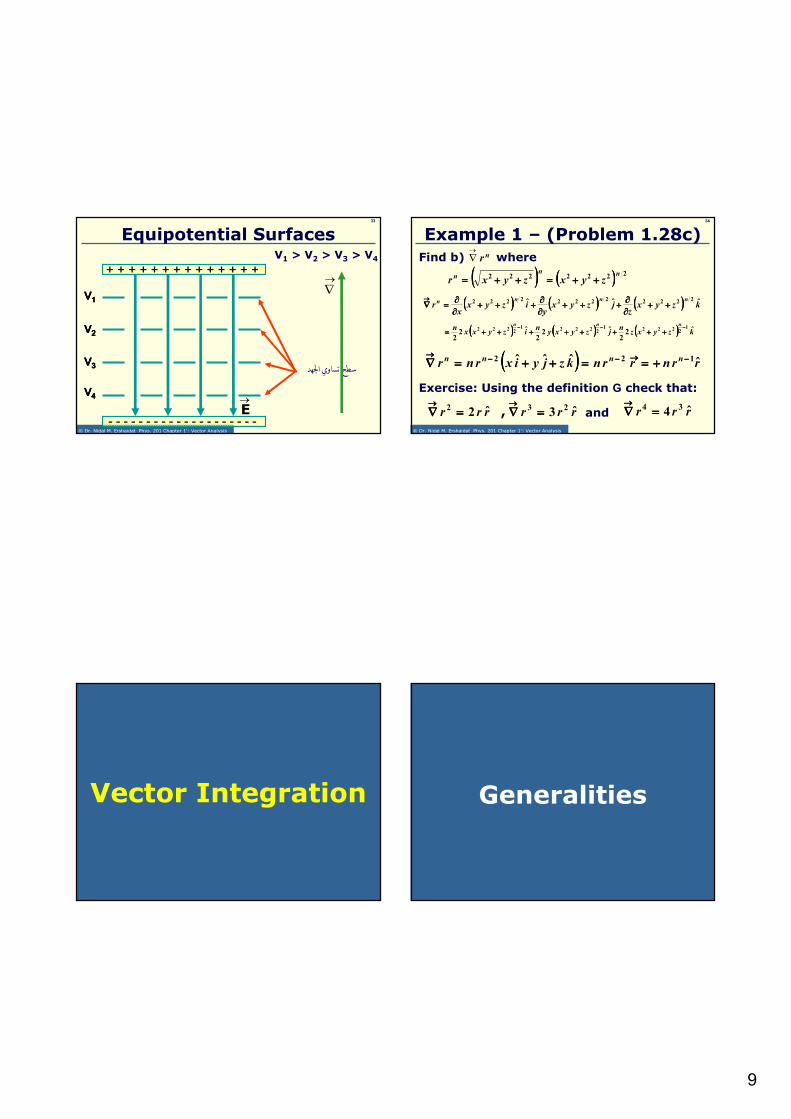
33
Equipotential Surfaces
VVVV1111
VVVV2222
VVVV3333
VVVV4444
!( )$ *+,
+ + + + + + + + + + + + + + + + + + + + + + + + + + + +
-- -- -- -- -- -- -- -- -- -- -- -- -- -- -- -- -- -- -- --
→E
→∇
V1 > V2 > V3 > V4
© Dr. Nidal M. Ershaidat Phys. 201 Chapter 1': Vector Analysis
34
Find b) where
Example 1 – (Problem 1.28c)nr
→∇
(((( )))) (((( )))) 2222222 nnn
zyxzyxr ++++++++====++++++++====
(((( )))) (((( )))) (((( )))) kzyxzn
jzyxyn
izyxxn
nnn
ˆ22
ˆ22
ˆ22
122221
222212222 −−−−−−−−−−−−
++++++++++++++++++++++++++++++++====
(((( )))) (((( )))) (((( )))) kzyxz
jzyxy
izyxx
rnnnn ˆˆˆ 222222222222 ++++++++
∂∂∂∂∂∂∂∂++++++++++++
∂∂∂∂∂∂∂∂++++++++++++
∂∂∂∂∂∂∂∂====∇∇∇∇
→→→→
(((( )))) rrnrrnkzjyixrnr nnnn ˆˆˆˆ 122 −−−−→→→→−−−−−−−−→→→→++++========++++++++====∇∇∇∇
Exercise: Using the definition G check that:
rrr ˆ22 ====∇∇∇∇→→→→
rrr ˆ3 23 ====∇∇∇∇→→→→
, rrr ˆ4 34 ====∇∇∇∇→→→→
and
Vector Integration Generalities
10
© Dr. Nidal M. Ershaidat Phys. 201 Chapter 1': Vector Analysis
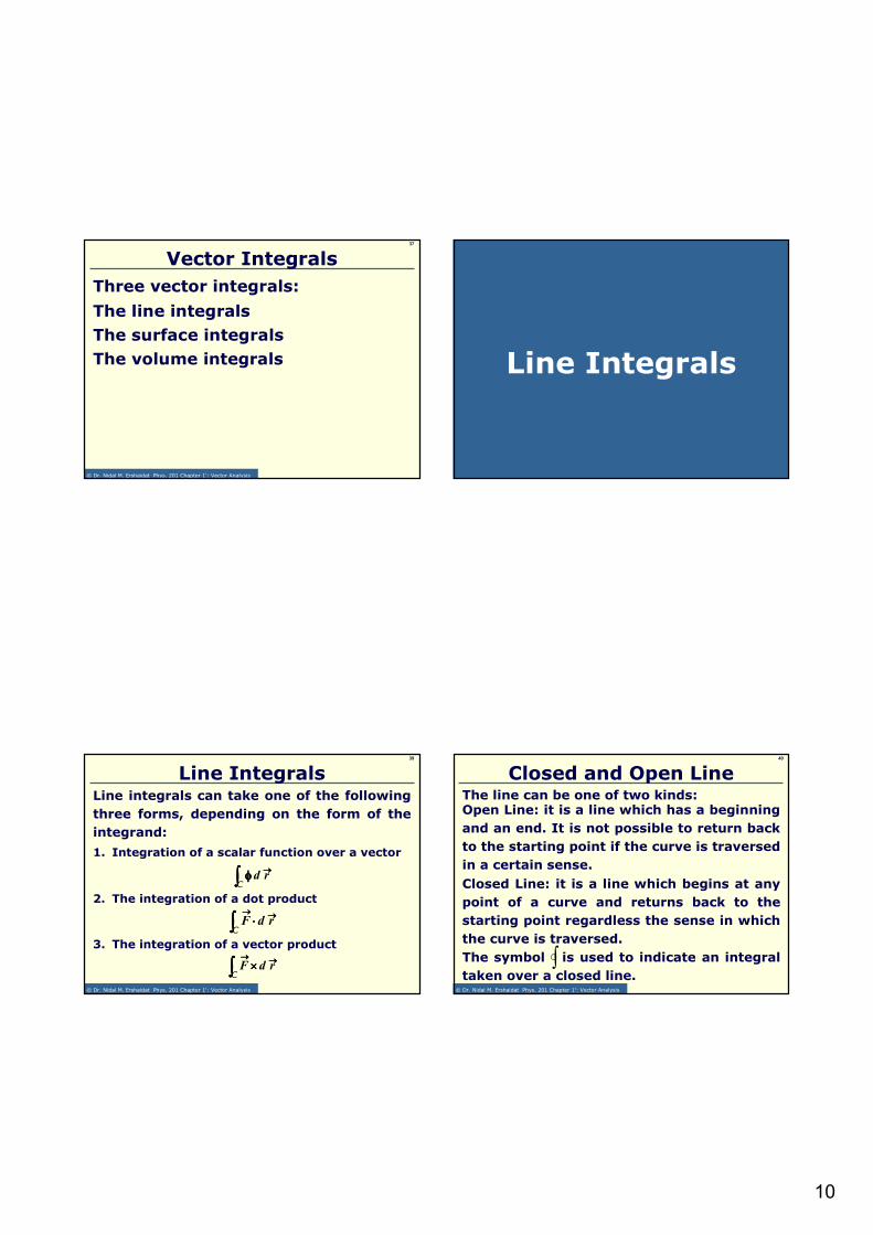
37
Three vector integrals:
Vector Integrals
The line integrals
The surface integrals
The volume integrals Line Integrals
© Dr. Nidal M. Ershaidat Phys. 201 Chapter 1': Vector Analysis
39
Line integrals can take one of the following
three forms, depending on the form of the
integrand:
Line Integrals
1. Integration of a scalar function over a vector
∫∫∫∫→→→→φφφφ
C
rd
2. The integration of a dot product
∫∫∫∫→→→→→→→→
⋅⋅⋅⋅C
rdF
3. The integration of a vector product
∫∫∫∫→→→→→→→→
××××C
rdF
© Dr. Nidal M. Ershaidat Phys. 201 Chapter 1': Vector Analysis
40
The line can be one of two kinds:
Closed and Open Line
Open Line: it is a line which has a beginning
and an end. It is not possible to return back
to the starting point if the curve is traversed
in a certain sense.
Closed Line: it is a line which begins at any
point of a curve and returns back to the
starting point regardless the sense in which
the curve is traversed.
The symbol is used to indicate an integral
taken over a closed line.∫
11
© Dr. Nidal M. Ershaidat Phys. 201 Chapter 1': Vector Analysis
41
∫∫∫∫ φφφφ drThe integral can be written as∫∫∫∫
→→→→φφφφC
rd
The result is obtained by evaluating the 3
integrals over the path C which should be
defined.
Generally the result depends on the path
taken.
→→→→
(((( ))))∫∫∫∫∫∫∫∫ ++++++++φφφφ====φφφφ →→→→
CC
zdkydjxdird ˆˆˆ
∫∫∫ φ+φ+φ=CCC
zkyjxi dˆdˆdˆ
© Dr. Nidal M. Ershaidat Phys. 201 Chapter 1': Vector Analysis
42
Example ∫∫∫∫ φφφφdr – Problem (1.35)
Evaluate the line integral ( )∫ ++C
zyxxy dd2d2
Where C connects the two points (0,0,0) and (1,1,1):
a) Along a straight line from (0,0,0) to (1,0,0) to (1,0,1)
to (1,1,1)
→→→→
( )∫ ++1
dd2d2
Czyxxy ( )∫ ++=
)0,0,1(
)0,0,0(
2 dd2d zyxxy
( )∫ +++)1,0,1(
)0,0,1(
2 dd2d zyxxy
( )∫ +++)1,1,1(
)1,0,1(
2 dd2d zyxxy
Solution: We shall call this path C1
© Dr. Nidal M. Ershaidat Phys. 201 Chapter 1': Vector Analysis
43
We actually have 9 integrals to be evaluated:
Problem (1.35) – Solution1
( )∫ ++=),,(
),,(A dzdyxdxyI
001
000
22
I1 = 0 because y = 0
I2 = 0 because we are integrating over y and y = 0
I3 = 0 because we are integrating over z and z = 0
2
001
000
2
I
z,y,x
z,y,xdyx∫
===
===+
3
001
000
I
z,y,x
z,y,xdz∫
===
===+
1
001
000
2
I
z,y,x
z,y,xdxy∫
===
====
© Dr. Nidal M. Ershaidat Phys. 201 Chapter 1': Vector Analysis
44
Problem (1.35) – Solution2
( )
654
101
001
101
001
101
001
2
101
001
2
2
2
I
,zy,x
,zy,x
I
z,y,x
z,y,x
I
z,y,x
z,y,x
),,(
),,(B
dzdyxdxy
dzdyxdxyI
∫∫∫
∫===
===
===
===
===
===++=
++=
I4 = 0 because y = 0 and we are integrating over x
and x = 1,
I5 = 0 because we are integrating over y and y = 0 ,
11
0
101
0016
=== ∫===
===zdzI
,zy,x
,zy,x

12
© Dr. Nidal M. Ershaidat Phys. 201 Chapter 1': Vector Analysis
45
Problem (1.35) – Solution3
( )
987
111
101
111
101
111
101
2
111
101
2
2
2
I
,zy,x
,zy,x
I
z,y,x
z,y,x
I
z,y,x
z,y,x
),,(
),,(C
dzdyxdxy
dzdyxdxyI
∫∫∫
∫===
===
===
===
===
===++=
++=
I7 = 0 – same argument as for I4.
I9 = 0 because we are integrating over z and z = 1
111
0
111
1018
=×== ∫===
===ydyxI
,zy,x
,zy,x
Result: IA + IB + IC = 3
© Dr. Nidal M. Ershaidat Phys. 201 Chapter 1': Vector Analysis
46
Example ∫∫∫∫ φφφφdr – Problem (1.35b)
Evaluate the line integral ( )∫ ++2
22
Cdzdyxdxy
Where C2 connects the two points (0,0,0) and (1,1,1):
b) Along a straight line from (0,0,0) to (1,1,1)
→→→→
( )∫ ++2
22
Cdzdyxdxy ( )∫ ++=
),,(
),,(dzdyxdxy
111
000
22
Solution
In order to evaluate the previous integral we
need the equation of the line.
The equation of the line is x = y = z
Which means that we can write dx = dy = dz
© Dr. Nidal M. Ershaidat Phys. 201 Chapter 1': Vector Analysis
47
Problem (1.35b) – Solution
1
0
1
0
21
0
3
22
3z
xy++=
∫∫∫ ++=222
22
CCCdzdxxdyy
3
711
3
1=++=
( )∫ ++2
22
Cdzdyxdxy
The integral can be written as:
Note that ( )∫1C⋯ ( )∫≠
2C⋯
© Dr. Nidal M. Ershaidat Phys. 201 Chapter 1': Vector Analysis
48
The integral is a scalar integral.
If the dependence of on x, y and z is known,
the integral is a classical scalar integral.
∫∫∫∫ F . dr - Work
→→→→F
→→→→→→→→
∫∫∫∫→→→→→→→→
⋅⋅⋅⋅C
rdF
The work done by a force on a system causing
a displacement of the system is given by:→rd
→→→→F
∫∫∫∫→→→→→→→→
⋅⋅⋅⋅====C
rdFW
Generally the result depends on the path
taken. If W is independent of the path then we
conclude that is a conservative force.→→→→F
13
Surface Integrals
© Dr. Nidal M. Ershaidat Phys. 201 Chapter 1': Vector Analysis
50
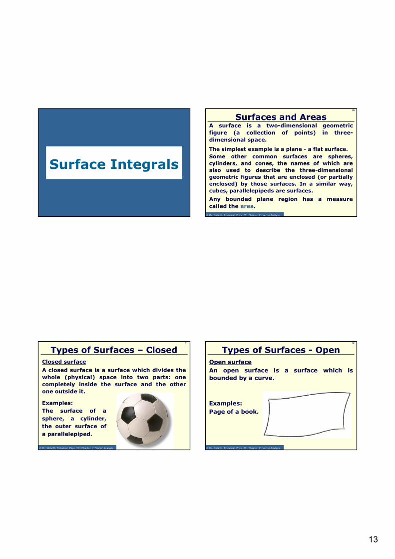
A surface is a two-dimensional geometric
figure (a collection of points) in three-
dimensional space.
Surfaces and Areas
The simplest example is a plane - a flat surface.
Some other common surfaces are spheres,
cylinders, and cones, the names of which are
also used to describe the three-dimensional
geometric figures that are enclosed (or partially
enclosed) by those surfaces. In a similar way,
cubes, parallelepipeds are surfaces.
Any bounded plane region has a measure
called the area.
© Dr. Nidal M. Ershaidat Phys. 201 Chapter 1': Vector Analysis
51
Types of Surfaces – Closed
Closed surface
Examples:
The surface of a
sphere, a cylinder,
the outer surface of
a parallelepiped.
A closed surface is a surface which divides the
whole (physical) space into two parts: one
completely inside the surface and the other
one outside it.
© Dr. Nidal M. Ershaidat Phys. 201 Chapter 1': Vector Analysis
52
Types of Surfaces - Open
Open surface
Examples:
Page of a book.
An open surface is a surface which is
bounded by a curve.
14
© Dr. Nidal M. Ershaidat Phys. 201 Chapter 1': Vector Analysis
53
θθθθ
In many cases in physics we need to deal with
surfaces. And we often need to determine the
normal to a surface.
We have seen, when we studied the vector
products, that the area is considered as a
vector whose magnitude is the area and its
direction is normal to the area.
Normal to a Surface
→AFor a parallelogram the area is
represented by the vector →A
→b
→c
is nothing else but the cross
product : (see figure)→→
× cb
→A
© Dr. Nidal M. Ershaidat Phys. 201 Chapter 1': Vector Analysis
54
The direction of the normal to a surface
depends on the type of surface.
Direction of the Normal to a Surface
For a closed surface the (positive) normal at a
certain element on the surface is taken
conventionally to point outward.
© Dr. Nidal M. Ershaidat Phys. 201 Chapter 1': Vector Analysis
56
When you curl the fingers of your right hand in
the direction of traversing the perimeter of the
element then the thumb ( ام) will point in the
positive direction of .n
Direction of the Normal to a SurfaceThe figure shows a surface element of an open
surface. The vector is a unit vector normal to the
surface at the location of the area element da and
its direction is defined using a right-hand rule.
n
n
© Dr. Nidal M. Ershaidat Phys. 201 Chapter 1': Vector Analysis
57
The flux of a vector is a surface integral.
Surface Integral in Physics
The most famous example is that of Gauss’s law
in electromagnetism.
∫ ⋅=Φ→
danA
Gauss’s law states that the flux of the electric
field from a closed surface is proportional to the
charge Q enclosed inside the surface, i.e.
ε
QAEdanE enc
AA====⋅⋅⋅⋅====⋅⋅⋅⋅ ∫∫∫∫∫∫∫∫
→→→→→→→→→→→→ˆ
Where εεεε is the permittivity.
The flux of vector is given by:→A
15
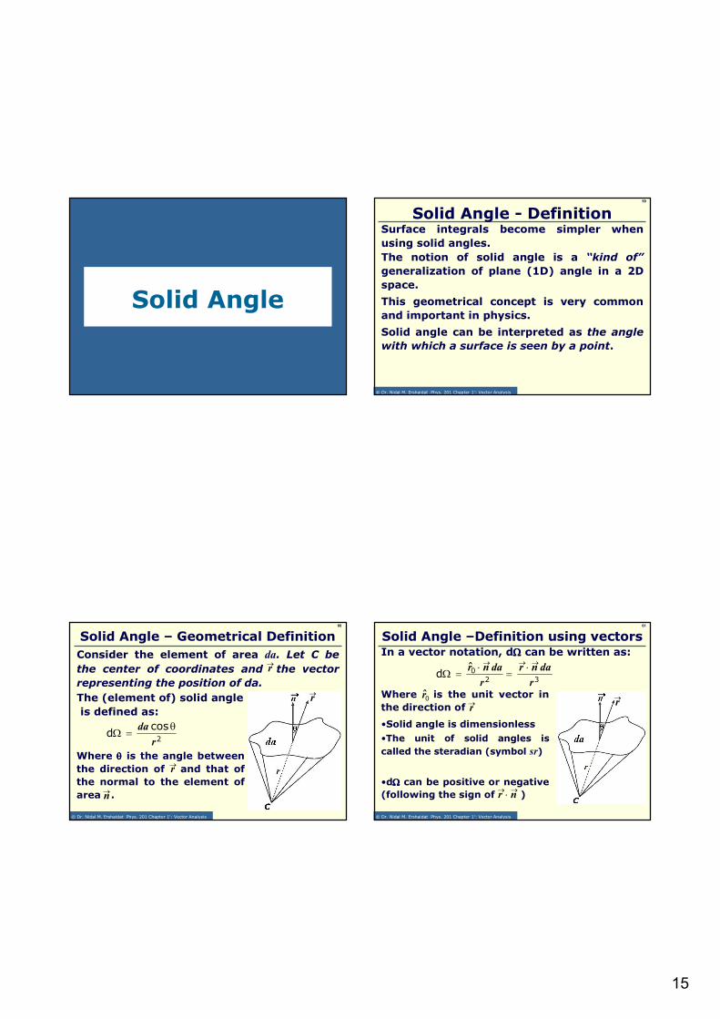
Solid Angle
© Dr. Nidal M. Ershaidat Phys. 201 Chapter 1': Vector Analysis
59
Surface integrals become simpler when
using solid angles.
Solid Angle - Definition
The notion of solid angle is a “kind of”
generalization of plane (1D) angle in a 2D
space.
Solid angle can be interpreted as the angle
with which a surface is seen by a point.
This geometrical concept is very common
and important in physics.
© Dr. Nidal M. Ershaidat Phys. 201 Chapter 1': Vector Analysis
60
Consider the element of area da. Let C be
the center of coordinates and the vector
representing the position of da.
Solid Angle – Geometrical Definition
The (element of) solid angle
is defined as:
2
cosd
r
da θ=Ω
Where θθθθ is the angle between
the direction of and that of
the normal to the element of
area .→n
→r
→r
→r
© Dr. Nidal M. Ershaidat Phys. 201 Chapter 1': Vector Analysis
61
In a vector notation, dΩΩΩΩ can be written as:
Solid Angle –Definition using vectors
20dr
danr→⋅
=Ω
Where is the unit vector in
the direction of→r
0r →r
3r
danr→→ ⋅
=
•Solid angle is dimensionless
•dΩΩΩΩ can be positive or negative
(following the sign of )→→ ⋅ nr
•The unit of solid angles is
called the steradian (symbol sr)
16
© Dr. Nidal M. Ershaidat Phys. 201 Chapter 1': Vector Analysis
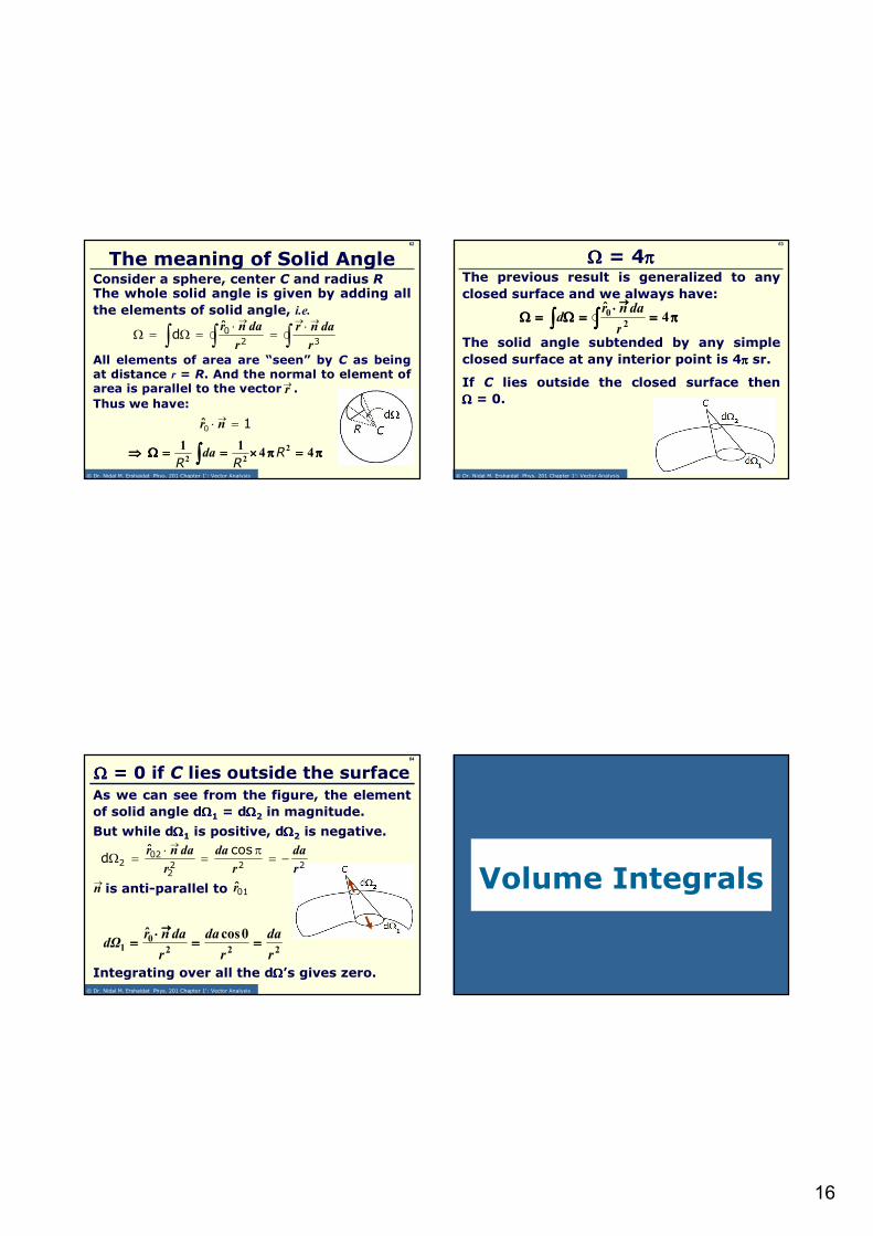
62
Consider a sphere, center C and radius R
The meaning of Solid Angle
∫∫→⋅
=Ω=Ω2
0dr
danr
The whole solid angle is given by adding all
the elements of solid angle, i.e.
ππππ====ππππ××××========ΩΩΩΩ⇒⇒⇒⇒ ∫∫∫∫ 4411 2
22R
RRda
10 =⋅ →nr
All elements of area are “seen” by C as being at distance r = R. And the normal to element of area is parallel to the vector .
Thus we have:
→r
∫→→ ⋅
=3r
danr
© Dr. Nidal M. Ershaidat Phys. 201 Chapter 1': Vector Analysis
63
The previous result is generalized to any
closed surface and we always have:
ΩΩΩΩ = 4ππππ
ππππ====⋅⋅⋅⋅
====ΩΩΩΩ====ΩΩΩΩ ∫∫∫∫∫∫∫∫→→→→
4ˆ
20
r
danrd
The solid angle subtended by any simple
closed surface at any interior point is 4ππππ sr.
If C lies outside the closed surface then
ΩΩΩΩ = 0.
© Dr. Nidal M. Ershaidat Phys. 201 Chapter 1': Vector Analysis
64
2220
1
0cosˆ
r
da
r
da
r
danrdΩ ========
⋅⋅⋅⋅====
→→→→
As we can see from the figure, the element
of solid angle dΩΩΩΩ1 = dΩΩΩΩ2 in magnitude.
ΩΩΩΩ = 0 if C lies outside the surface
But while dΩΩΩΩ1 is positive, dΩΩΩΩ2 is negative.
is anti-parallel to →n 01r
2222
022
cosˆd
r
da
r
da
r
danr−=
π=
⋅=Ω
→
Integrating over all the dΩΩΩΩ’s gives zero.
Volume Integrals
17
© Dr. Nidal M. Ershaidat Phys. 201 Chapter 1': Vector Analysis
67
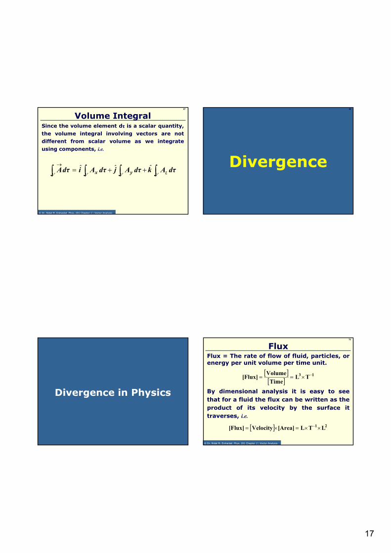
Since the volume element dττττ is a scalar quantity,
the volume integral involving vectors are not
different from scalar volume as we integrate
using components, i.e.
Volume Integral
∫∫∫∫ ++=→
Vz
Vy
Vx
VdτAkdτAjdτAidτA ˆˆˆ
68
Divergence
Divergence in Physics
© Dr. Nidal M. Ershaidat Phys. 201 Chapter 1': Vector Analysis
70
Flux = The rate of flow of fluid, particles, or energy per unit volume per time unit.
Flux
[ ][ ]
13TL
Time
Volume[Flux]
−×==
By dimensional analysis it is easy to see
that for a fluid the flux can be written as the
product of its velocity by the surface it
traverses, i.e.
[ ] 21 LTL[Area]Velocity[Flux] ××=×= −
18
© Dr. Nidal M. Ershaidat Phys. 201 Chapter 1': Vector Analysis
71
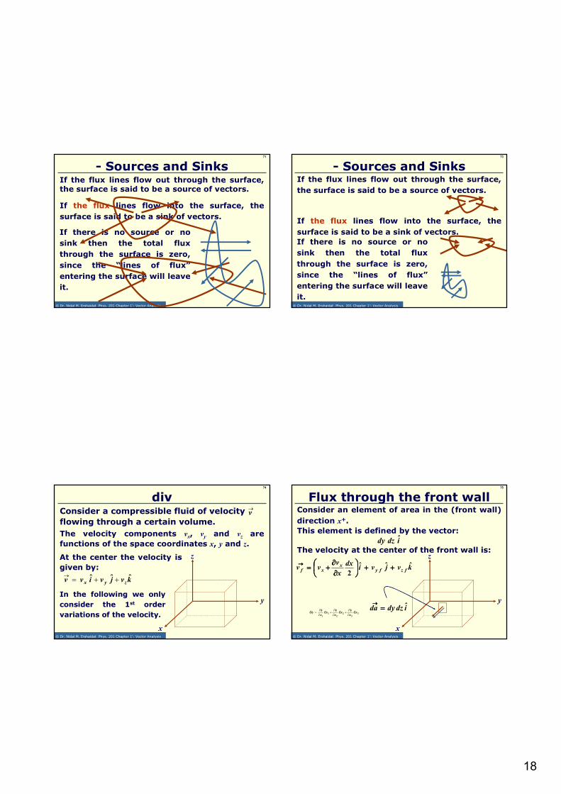
If there is no source or no
sink then the total flux
through the surface is zero,
since the “lines of flux”
entering the surface will leave
it.
If the flux lines flow out through the surface, the surface is said to be a source of vectors.
- Sources and Sinks
If the flux lines flow into the surface, the
surface is said to be a sink of vectors.
© Dr. Nidal M. Ershaidat Phys. 201 Chapter 1': Vector Analysis
73
If there is no source or no
sink then the total flux
through the surface is zero,
since the “lines of flux”
entering the surface will leave
it.
If the flux lines flow out through the surface,
the surface is said to be a source of vectors.
- Sources and Sinks
If the flux lines flow into the surface, the
surface is said to be a sink of vectors.
© Dr. Nidal M. Ershaidat Phys. 201 Chapter 1': Vector Analysis
74
y
x
z
Consider a compressible fluid of velocity
flowing through a certain volume.
div
The velocity components vx, vy and vz are
functions of the space coordinates x, y and z.
At the center the velocity is
given by:
kvjvivv zyxˆˆˆ ++=
→
→v
In the following we only
consider the 1st order
variations of the velocity.
© Dr. Nidal M. Ershaidat Phys. 201 Chapter 1': Vector Analysis
75
Consider an element of area in the (front wall)
direction x+.
Flux through the front wall
This element is defined by the vector:
The velocity at the center of the front wall is:
izdyd ˆ
y
x
z
kvjvixd
x
vvv fzfy
xxf
ˆˆˆ2
++++++++
∂∂∂∂∂∂∂∂
++++====→→→→
izdydda ˆ====→→→→
33
22
11
dddd xx
xx
xx ∂
φ∂+
∂φ∂
+∂
φ∂=φ

19
© Dr. Nidal M. Ershaidat Phys. 201 Chapter 1': Vector Analysis
76
The flux through the front wall is:
izdydkvjvidx
x
vvF fzfy
xxf
ˆˆˆˆ2
⋅⋅⋅⋅
++++++++
∂∂∂∂∂∂∂∂
++++====
Flux through the front wall
y
x
zzdyddx
x
vv xx
∂∂∂∂∂∂∂∂
++++====2
© Dr. Nidal M. Ershaidat Phys. 201 Chapter 1': Vector Analysis
77
Flux through the back wallThe element of area in the back wall is defined
by the vector:
(((( ))))izdydkvjvidx
x
vvF bzby
xxb
ˆˆˆˆ2
−−−−⋅⋅⋅⋅
++++++++
∂∂∂∂
∂∂∂∂−−−−====
The velocity at the center of the back wall is:
idzyd ˆ−−−−
kvjvidx
x
vvv bzby
xxb
ˆˆˆ2
++++++++
∂∂∂∂∂∂∂∂
−−−−====→→→→
The flux through the back
wall is:
zdyddx
x
vv xx
∂∂∂∂∂∂∂∂
++++−−−−====2
© Dr. Nidal M. Ershaidat Phys. 201 Chapter 1': Vector Analysis
78
zdydxdz
vF ztbnet ∂∂∂∂
∂∂∂∂====
zdydxdx
vx
∂∂∂∂∂∂∂∂
====
The net flux is:
Net Flux
In a similar manner one can prove that the net
flux through the top and bottom sides and the
net flux through the left and right sides are,
respectively, given by:
zdydxdy
vF
yrlnet ∂∂∂∂
∂∂∂∂====
zdyddx
x
vvzdyd
dx
x
vvF x
xx
xfbnet
∂∂∂∂∂∂∂∂
++++−−−−++++
∂∂∂∂∂∂∂∂
++++====22
and
© Dr. Nidal M. Ershaidat Phys. 201 Chapter 1': Vector Analysis
79
z
v
y
v
x
v zyx
∂∂∂∂
∂∂∂∂++++
∂∂∂∂
∂∂∂∂++++
∂∂∂∂∂∂∂∂
The net flux through the small volume dxdydz
is:
Net Flux through the small volume
which also represents the outgoing flux per
unit volume.
z
v
y
v
x
v zyx
∂∂∂∂
∂∂∂∂++++
∂∂∂∂
∂∂∂∂++++
∂∂∂∂∂∂∂∂ can be written in a vector form as:
z
v
y
v
x
vv
zyx
∂∂∂∂
∂∂∂∂++++
∂∂∂∂
∂∂∂∂++++
∂∂∂∂∂∂∂∂
====⋅⋅⋅⋅∇∇∇∇→→→→→→→→
Which we call the divergence of the vector .→v
We sometimes also write div→v
20
© Dr. Nidal M. Ershaidat Phys. 201 Chapter 1': Vector Analysis
80
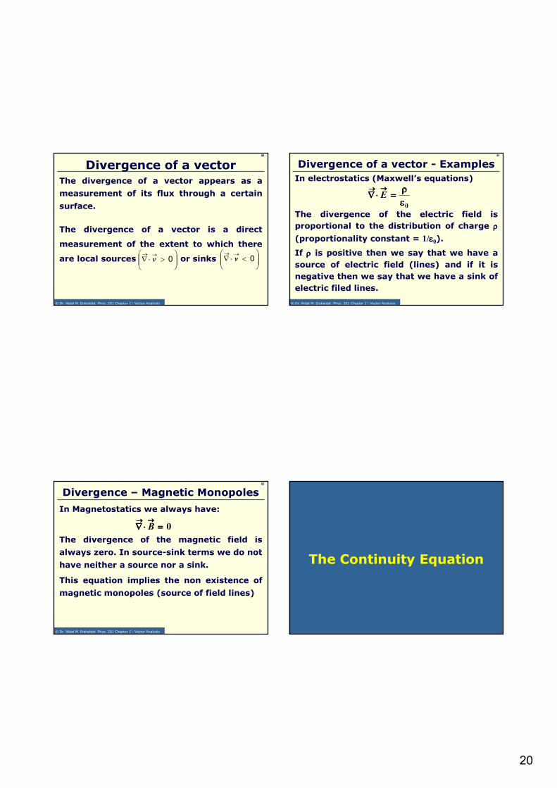
The divergence of a vector appears as a
measurement of its flux through a certain
surface.
The divergence of a vector is a direct
measurement of the extent to which there
are local sources or sinks
Divergence of a vector
<⋅∇
→→0v
>⋅∇
→→0v
© Dr. Nidal M. Ershaidat Phys. 201 Chapter 1': Vector Analysis
81
In electrostatics (Maxwell’s equations)
The divergence of the electric field is
proportional to the distribution of charge ρρρρ
(proportionality constant = 1/εεεε0).
Divergence of a vector - Examples
0εεεερρρρ
====⋅⋅⋅⋅∇∇∇∇→→→→→→→→E
If ρρρρ is positive then we say that we have a
source of electric field (lines) and if it is
negative then we say that we have a sink of
electric filed lines.
© Dr. Nidal M. Ershaidat Phys. 201 Chapter 1': Vector Analysis
82
In Magnetostatics we always have:
The divergence of the magnetic field is
always zero. In source-sink terms we do not
have neither a source nor a sink.
Divergence – Magnetic Monopoles
0====⋅⋅⋅⋅∇∇∇∇→→→→→→→→B
This equation implies the non existence of
magnetic monopoles (source of field lines)
The Continuity Equation

21
© Dr. Nidal M. Ershaidat Phys. 201 Chapter 1': Vector Analysis
84
The net flux of velocity through the volume is:
If ρρρρ(t) is the density of the fluid at instant t,
then the net flux of mass per unit time through
the volume is:
The Continuity Equation
ττττ⋅⋅⋅⋅∇∇∇∇→→→→→→→→dv
ττττρρρρ⋅⋅⋅⋅∇∇∇∇→→→→→→→→dv )(
equals strictly the decrease of mass
per unit time, i.e. Which gives:
ττττρρρρ⋅⋅⋅⋅∇∇∇∇→→→→→→→→dv )(
ττττ∂∂∂∂ρρρρ∂∂∂∂−−−− dt
)(→→→→→→→→
ρρρρ⋅⋅⋅⋅∇∇∇∇ v 0====∂∂∂∂ρρρρ∂∂∂∂++++t
This equation is called the continuity equation.
© Dr. Nidal M. Ershaidat Phys. 201 Chapter 1': Vector Analysis
85
Prove that
a)
Example – Problem 1.38
→→→→→→⋅∇φ+⋅φ∇=φ⋅∇ AAA
( )kjikz
jy
ix
zyxˆˆˆˆˆˆ AAAA φ+φ+φ⋅
∂∂
+∂∂
+∂∂
=φ⋅∇→→
( ) ( ) ( )zyxzyxAAA φ
∂∂
+φ∂∂
+φ∂∂
=
∂φ∂
+∂φ∂
+∂φ∂
= zyxzyxAAA
∂
∂φ+
∂
∂φ+
∂∂
φzyx
zyx AAA
→→⋅φ∇ A
→→⋅∇φ A
+
+=
Solution:
© Dr. Nidal M. Ershaidat Phys. 201 Chapter 1': Vector Analysis
86
Example – Problem 1.38Prove that
b)→→→→→→→→→→→→→→→→→→→→→→→→→→→→
⋅⋅⋅⋅∇∇∇∇++++⋅⋅⋅⋅∇∇∇∇====
++++⋅⋅⋅⋅∇∇∇∇ BABA
We leave the proof as an exercise.
See also exercises 1.18 and 1.19
87
z
v
y
v
x
v zyx
∂
∂+
∂
∂+
∂∂
We saw that the outgoing flux per volume unit
is:
Net Flux and divergence
And the flux through a surface Si limiting an
element of volume dττττi is given by:
For a finite volume V limited by a finite surface
S, we have:
∫→→
⋅iS
iav d
→→⋅∇= v
iv τ⋅∇=→→
d
In other words we have:
∫→→
⋅iS
iav d
∫∫∫∫∫∫∫∫ ττττ⋅⋅⋅⋅∇∇∇∇====⋅⋅⋅⋅→→→→→→→→→→→→→→→→
Vdvadv
S

22
© Dr. Nidal M. Ershaidat Phys. 201 Chapter 1': Vector Analysis
88
The previous relation is called the Gauss’s
divergence theorem
Gauss’s divergence theorem
This theorem is valid even if the volume is
multiply connected i.e., even it has holes in it.
In such cases the surface integral is taken over
the sum of the surface bounding the volume.
∫∫ τ⋅∇=⋅→→→→
V
dd vavS
The integral at the lhs must be taken only on
the outer surface limiting the volume V. Simply
because the integration on the elements of the
interior of V cancel in pairs.
89
Evaluate Over the unit cube defined by the
point (0,0,0) and the point intercepts on the positive
x, y and z axes.
y(0,1,0)
x
(1,0,0)
(0,0,1)
z
Example 3 (see Example 1.20)
∫∫∫∫→→→→→→→→
⋅⋅⋅⋅S
adr
(0,0,0)
© Dr. Nidal M. Ershaidat Phys. 201 Chapter 1': Vector Analysis
90
Example 3 –Solution Solution:
∫∫∫∫→→→→→→→→
⋅⋅⋅⋅ adr ∫∫∫∫∫∫∫∫→→→→→→→→→→→→→→→→
⋅⋅⋅⋅++++⋅⋅⋅⋅====wallbackwallfront
adradr
∫∫∫∫∫∫∫∫→→→→→→→→→→→→→→→→
⋅⋅⋅⋅++++⋅⋅⋅⋅++++wallbottomwalltop
adradr
∫∫∫∫∫∫∫∫→→→→→→→→→→→→→→→→
⋅⋅⋅⋅++++⋅⋅⋅⋅++++wallleftwallright
adradr
© Dr. Nidal M. Ershaidat Phys. 201 Chapter 1': Vector Analysis
91
Front and Back Walls
(((( )))) idzdykzjyixdrwallfront
ˆˆˆˆa
1
0
1
0
⋅⋅⋅⋅++++++++====⋅⋅⋅⋅ ∫∫∫∫ ∫∫∫∫∫∫∫∫→→→→→→→→
(((( )))) (((( )))) 0ˆˆˆˆ0
1
0
1
0
====−−−−++++++++====⋅⋅⋅⋅ ∫∫∫∫ ∫∫∫∫∫∫∫∫→→→→→→→→
idzdykzjyiadrwallback
i
11
1
0
1
0
1
0
1
0
====××××======== ∫∫∫∫∫∫∫∫∫∫∫∫ ∫∫∫∫ dzdydzdyx
23
© Dr. Nidal M. Ershaidat Phys. 201 Chapter 1': Vector Analysis
92
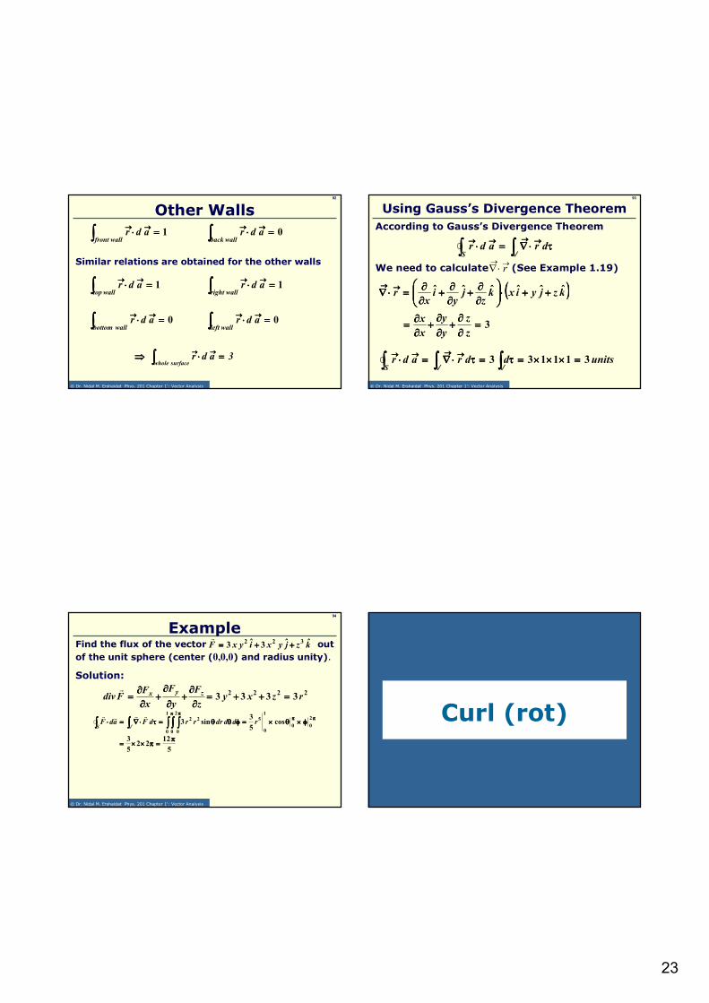
Other Walls
1====⋅⋅⋅⋅∫∫∫∫→→→→→→→→
walltopadr
0====⋅⋅⋅⋅∫∫∫∫→→→→→→→→
wallbottomadr
1====⋅⋅⋅⋅∫∫∫∫→→→→→→→→
wallrightadr
0====⋅⋅⋅⋅∫∫∫∫→→→→→→→→
wallleftadr
Similar relations are obtained for the other walls
0====⋅⋅⋅⋅∫∫∫∫→→→→→→→→
wallbackadr1====⋅⋅⋅⋅∫∫∫∫
→→→→→→→→
wallfrontadr
3adreurfacswhole
====⋅⋅⋅⋅⇒⇒⇒⇒ ∫∫∫∫→→→→→→→→
© Dr. Nidal M. Ershaidat Phys. 201 Chapter 1': Vector Analysis
93
Using Gauss’s Divergence Theorem
∫∫∫∫∫∫∫∫ ττττ⋅⋅⋅⋅∇∇∇∇====⋅⋅⋅⋅→→→→→→→→→→→→→→→→
V
dradrS
We need to calculate (See Example 1.19)→→
⋅∇ r
(((( ))))kzjyixkz
jy
ix
r ˆˆˆˆˆˆ ++++++++⋅⋅⋅⋅
∂∂∂∂∂∂∂∂++++
∂∂∂∂∂∂∂∂++++
∂∂∂∂∂∂∂∂====⋅⋅⋅⋅∇∇∇∇
→→→→→→→→
3====∂∂∂∂∂∂∂∂
++++∂∂∂∂∂∂∂∂
++++∂∂∂∂∂∂∂∂====
z
z
y
y
x
x
According to Gauss’s Divergence Theorem
unitsddradrS
311133 ====××××××××××××====ττττ====ττττ⋅⋅⋅⋅∇∇∇∇====⋅⋅⋅⋅ ∫∫∫∫∫∫∫∫∫∫∫∫→→→→→→→→→→→→→→→→
VV
© Dr. Nidal M. Ershaidat Phys. 201 Chapter 1': Vector Analysis
94
Find the flux of the vector out
of the unit sphere (center (0,0,0) and radius unity).
Example
Solution:
22223333 rzxy
z
F
y
F
x
FFdiv zyx ====++++++++====
∂∂∂∂
∂∂∂∂++++
∂∂∂∂
∂∂∂∂++++
∂∂∂∂∂∂∂∂
====
kzjyxiyxF ˆˆ3ˆ3322 ++++++++====
5
1222
5
3
cos5
3sin3
2
00
1
0
51
0 0
2
0
22
ππππ====ππππ××××××××====
φφφφ××××θθθθ××××====φφφφθθθθθθθθ====ττττ⋅⋅⋅⋅∇∇∇∇====⋅⋅⋅⋅ππππππππ
ππππ ππππ
∫∫∫∫ ∫∫∫∫ ∫∫∫∫∫∫∫∫∫∫∫∫ rdddrrrdFadFV
S
Curl (rot)

24
© Dr. Nidal M. Ershaidat Phys. 201 Chapter 1': Vector Analysis
101
is a vector:
Curl (rot) is a vector
zyx FFF
zyx
kji
F∂∂∂∂∂∂∂∂
∂∂∂∂∂∂∂∂
∂∂∂∂∂∂∂∂
====××××∇∇∇∇→→→→→→→→
ˆˆˆ
→→→→→→→→××××∇∇∇∇ F
Note: if then the vector is said to be irrotational.→→→→F0====××××∇∇∇∇
→→→→→→→→F
The curl is related to the measurement of the
“strength” of rotation of a vector at a point in
space.
and we call it curl or rot →→→→F
→→→→F
© Dr. Nidal M. Ershaidat Phys. 201 Chapter 1': Vector Analysis
102
We can prove (in fluid mechanics) that
Flux of Curl (rot)
Important:
See examples 1.22 and 1.23 in the textbook
The line integral of vector around a closed
path is equal to the flux of its curl.
→→→→F
→→→→→→→→→→→→→→→→→→→→⋅⋅⋅⋅××××∇∇∇∇====⋅⋅⋅⋅∫∫∫∫ adFrdF
Stokes’ Theorem
© Dr. Nidal M. Ershaidat Phys. 201 Chapter 1': Vector Analysis
104
Stokes’ theorem states that:
Stokes’ Theorem
∫∫∫∫∫∫∫∫→→→→→→→→→→→→→→→→→→→→
⋅⋅⋅⋅====⋅⋅⋅⋅××××∇∇∇∇CS
dFadF ℓ
Where S is a surface bounded (limited) by a
curve C
Proof:
Let’s consider the surface in the
figure. Let’s divide the area into
differential (infinitesimal) area
elements

25
© Dr. Nidal M. Ershaidat Phys. 201 Chapter 1': Vector Analysis
105
Stokes’ Theorem - ProofFor the ith element of area the equation we
obtained in the previous paragraph can be written
here as: →→→→→→→→→→→→→→→→→→→→⋅⋅⋅⋅××××∇∇∇∇====⋅⋅⋅⋅∫∫∫∫ ii adFdF ℓ
∑∑∑∑∑∑∑∑∫∫∫∫→→→→→→→→→→→→→→→→→→→→
⋅⋅⋅⋅××××∇∇∇∇====⋅⋅⋅⋅i
i
i
i adFdF ℓ
∫∫∫∫∫∫∫∫→→→→→→→→→→→→→→→→→→→→
⋅⋅⋅⋅××××∇∇∇∇====⋅⋅⋅⋅SC
adFdF ℓ
Summation over all the area elements gives:
Which tends toward the limit when the number of
elements become large enough and the summation
becomes simply an integral, i.e.
© Dr. Nidal M. Ershaidat Phys. 201 Chapter 1': Vector Analysis
106
Stokes’ Theorem - Note
Note: When making the sum of the linear integral of the
vector the terms involving common boundaries between
the area elements will vanish because they cancel in
pairs.
∑∑∑∑∑∑∑∑∫∫∫∫→→→→→→→→→→→→→→→→→→→→
⋅⋅⋅⋅××××∇∇∇∇====⋅⋅⋅⋅i
i
i
i adFdF ℓ
∫∫∫∫∑∑∑∑∫∫∫∫→→→→→→→→→→→→→→→→
⋅⋅⋅⋅====⋅⋅⋅⋅C
i
i dFdF ℓℓ
© Dr. Nidal M. Ershaidat Phys. 201 Chapter 1': Vector Analysis
107
Stokes’ Theorem
Irish mathematician and physicist. Stokes
studied fluorescence and the luminiferous ether, questioning Young and Fresnel's ether drag theory. Stokes systematically studied fluid mechanics, elastic solids, waves in elastic media, and diffraction. In
fact, the basic equations of fluid mechanics are called the Navier-Stokes equations in his honor. He also formulated the three-dimensional analog of Green's theorem known as Stokes' theorem, and was a
pioneer in the use of divergent series.
Stokes, George (1819-1903)
The Laplacian
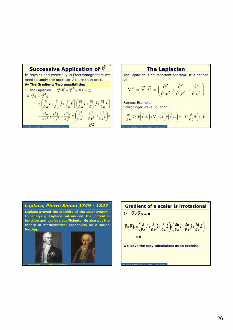
26
© Dr. Nidal M. Ershaidat Phys. 201 Chapter 1': Vector Analysis
109
In physics and especially in Electromagnetism we
need to apply the operator more than once.→∇
Successive Application of ∇∇∇∇
φ∇=φ∇⋅∇→→→ 2
→→→→
AA-- The Gradient: Two possibilitiesThe Gradient: Two possibilities
1- The Laplacian
2
2
2
2
2
2
zyx ∂φ∂
+∂
φ∂+
∂φ∂
=
∂φ∂
+∂φ∂
+∂φ∂
⋅
∂∂
+∂∂
+∂∂
= kz
jy
ix
kz
jy
ix
ˆˆˆˆˆˆ
φ
∂∂
+∂∂
+∂∂
=2
2
2
2
2
2
zyx
∆=∇=∇=∇⋅∇→→→
22
2∇ © Dr. Nidal M. Ershaidat Phys. 201 Chapter 1': Vector Analysis
110
The Laplacian is an important operator. It is defined
by:
The Laplacian
∂∂
+∂∂
+∂∂
=∇⋅∇=∇→→
2
2
2
2
2
22
zyx
Famous Example:
Schrödinger Wave Equation:
Ψ
∂∂
−=
Ψ
+
Ψ∇−
→→→→
t,rt
t,rt,rVt,r2
22
ℏℏ
im
© Dr. Nidal M. Ershaidat Phys. 201 Chapter 1': Vector Analysis
111
Laplace proved the stability of the solar system.
In analysis, Laplace introduced the potential
function and Laplace coefficients. He also put the
theory of mathematical probability on a sound
footing.
Laplace, Pierre Simon 1749 - 1827
© Dr. Nidal M. Ershaidat Phys. 201 Chapter 1': Vector Analysis
112
Gradient of a scalar is irrotational
0====
2-
∂∂∂∂φφφφ∂∂∂∂++++
∂∂∂∂φφφφ∂∂∂∂++++
∂∂∂∂φφφφ∂∂∂∂××××
∂∂∂∂∂∂∂∂++++
∂∂∂∂∂∂∂∂++++
∂∂∂∂∂∂∂∂====φφφφ∇∇∇∇××××∇∇∇∇
→→→→→→→→kz
jy
ix
kz
jy
ix
ˆˆˆˆˆˆ
0====φφφφ∇∇∇∇××××∇∇∇∇→→→→→→→→
We leave the easy calculations as an exercise.
27
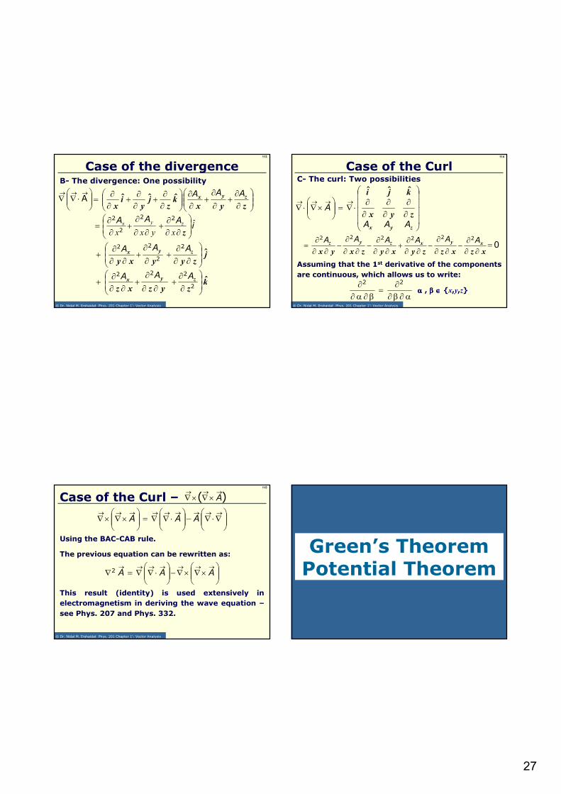
© Dr. Nidal M. Ershaidat Phys. 201 Chapter 1': Vector Analysis
113
B- The divergence: One possibility
Case of the divergence
⋅∇∇
→→→A
iAAA ˆ
∂∂∂
+∂∂
∂+
∂∂
=zxyxx
zyx22
2
2
∂
∂+
∂
∂+
∂∂
∂∂
+∂∂
+∂∂
=zyx
kz
jy
ix
zyx AAAˆˆˆ
jzyyxy
zyx ˆ2
2
22
∂∂
∂+
∂
∂+
∂∂∂
+AAA
kzyzxz
zyx ˆ2
222
∂
∂+
∂∂
∂+
∂∂∂
+AAA
© Dr. Nidal M. Ershaidat Phys. 201 Chapter 1': Vector Analysis
114
C- The curl: Two possibilities
Case of the Curl
∂∂
∂∂
∂∂
⋅∇=
×∇⋅∇
→→→→
zyx
zyx
kji
AAA
A
ˆˆˆ
xzxzzyxyzxyx
xyxzyz
∂∂∂
−∂∂
∂−
∂∂∂
+∂∂
∂−
∂∂
∂−
∂∂
∂=
AAAAAA 222222
0=
Assuming that the 1st derivative of the components
are continuous, which allows us to write:
α∂β∂∂
=β∂α∂
∂ 22
αααα , ββββ ∈∈∈∈ x,y,z
© Dr. Nidal M. Ershaidat Phys. 201 Chapter 1': Vector Analysis
115
Case of the Curl –
∇⋅∇−
⋅∇∇=
×∇×∇
→→→→→→→→→AAA
Using the BAC-CAB rule.
)(→→→
×∇×∇ A
×∇×∇−
⋅∇∇=∇
→→→→→→→AAA2
The previous equation can be rewritten as:
This result (identity) is used extensively in
electromagnetism in deriving the wave equation –
see Phys. 207 and Phys. 332.
Green’s TheoremPotential Theorem
28
© Dr. Nidal M. Ershaidat Phys. 201 Chapter 1': Vector Analysis
117
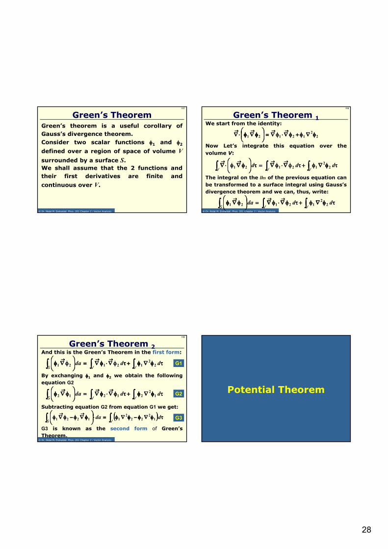
Green’s theorem is a useful corollary of
Gauss’s divergence theorem.
Consider two scalar functions φφφφ1 and φφφφ2
defined over a region of space of volume V
surrounded by a surface S.
We shall assume that the 2 functions and
their first derivatives are finite and
continuous over V.
Green’s Theorem
© Dr. Nidal M. Ershaidat Phys. 201 Chapter 1': Vector Analysis
118
We start from the identity:
Green’s Theorem 1
22
12121 φφφφ∇∇∇∇φφφφ++++φφφφ∇∇∇∇⋅⋅⋅⋅φφφφ∇∇∇∇====
φφφφ∇∇∇∇φφφφ⋅⋅⋅⋅∇∇∇∇
→→→→→→→→→→→→→→→→
Now Let’s integrate this equation over the
volume V:
∫∫∫∫∫∫∫∫∫∫∫∫ ττττφφφφ∇∇∇∇φφφφ++++ττττφφφφ∇∇∇∇⋅⋅⋅⋅φφφφ∇∇∇∇====ττττ
φφφφ∇∇∇∇φφφφ⋅⋅⋅⋅∇∇∇∇
→→→→→→→→→→→→→→→→
VVVddd 2
212121
The integral on the lhs of the previous equation can
be transformed to a surface integral using Gauss’s
divergence theorem and we can, thus, write:
∫∫∫∫∫∫∫∫∫∫∫∫ ττττφφφφ∇∇∇∇φφφφ++++ττττφφφφ∇∇∇∇⋅⋅⋅⋅φφφφ∇∇∇∇====
φφφφ∇∇∇∇φφφφ
→→→→→→→→→→→→
VVS
ddad 22
12121
© Dr. Nidal M. Ershaidat Phys. 201 Chapter 1': Vector Analysis
119
And this is the Green’s Theorem in the first form:
Green’s Theorem 2
∫∫∫∫∫∫∫∫∫∫∫∫ ττττφφφφ∇∇∇∇φφφφ++++ττττφφφφ∇∇∇∇⋅⋅⋅⋅φφφφ∇∇∇∇====
φφφφ∇∇∇∇φφφφ
→→→→→→→→→→→→
VVS
ddad 22
12121
By exchanging φφφφ1 and φφφφ2 we obtain the following
equation G2
∫∫∫∫∫∫∫∫∫∫∫∫ ττττφφφφ∇∇∇∇φφφφ++++ττττφφφφ∇∇∇∇⋅⋅⋅⋅φφφφ∇∇∇∇====
φφφφ∇∇∇∇φφφφ
→→→→→→→→→→→→
VVS
ddad 12
21212
G1
G2
Subtracting equation G2 from equation G1 we get:
(((( ))))∫∫∫∫∫∫∫∫ ττττφφφφ∇∇∇∇φφφφ−−−−φφφφ∇∇∇∇φφφφ====⋅⋅⋅⋅
φφφφ∇∇∇∇φφφφ−−−−φφφφ∇∇∇∇φφφφ
→→→→→→→→
VS
dad 12
222
11221 G3
G3 is known as the second form of of Green’s
Theorem.
Potential Theorem

29
© Dr. Nidal M. Ershaidat Phys. 201 Chapter 1': Vector Analysis
121
Consider a force which satisfies the equation:
Which means as we have said before that is
irrotational.
This suggests the existence of a scalar function
φφφφ such that:
In terms of gradient, the magnitude of the force
equals the magnitude of the gradient of the scalar
function φφφφ and its direction is the opposite
direction of this gradient. (See lecture on Gradient
and the negative sign)
Scalar Potential
0====××××∇∇∇∇→→→→→→→→F
We saw that , φφφφ being a scalar function,0====φφφφ∇∇∇∇××××∇∇∇∇→→→→→→→→
→→→→F
→→→→F
φφφφ∇∇∇∇−−−−====→→→→→→→→
F
© Dr. Nidal M. Ershaidat Phys. 201 Chapter 1': Vector Analysis
122
And the scalar function φφφφ that satisfies the
equation:
We have seen that such a force is said to be
conservative. According to the previous
discussion a force is conservative if it
satisfies the irrotational relation:
Alternatively we can associate to any force
satisfying the irrotational relation a scalar
function (which depends on space coordinates)
is called a scalar potential.
Scalar Potential
0====××××∇∇∇∇→→→→→→→→F
→→→→F
φφφφ∇∇∇∇−−−−====→→→→→→→→
F
© Dr. Nidal M. Ershaidat Phys. 201 Chapter 1': Vector Analysis
123
Using Stokes’ theorem
Conservative forces and Stokes’ Theorem
∫∫∫∫∫∫∫∫→→→→→→→→→→→→→→→→→→→→
⋅⋅⋅⋅××××∇∇∇∇====⋅⋅⋅⋅SC
adFrdF
0====⋅⋅⋅⋅∫∫∫∫→→→→→→→→
CrdF
Which means that the work done by a
conservative force over a closed path is zero.
We also equivalently say that the work done by
a conservative force does not depend on the
nature of the path but only on its initial and
final points.
gives in the case of a conservative force )( 0====××××∇∇∇∇→→→→→→→→F
© Dr. Nidal M. Ershaidat Phys. 201 Chapter 1': Vector Analysis
124
Tow kinds of potential appear in physics:
scalar potential and vector potential
In general the term potential includes the
effects of any external force (action) on a
given system.
We often express this influence in terms of
“potential energy”.
This energy is “stored” in the system and
when the external agent “leaves” the
system, the system uses the “potential
energy” to perform actions itself.
Scalar Potential

30
© Dr. Nidal M. Ershaidat Phys. 201 Chapter 1': Vector Analysis
125
We can create a vector potential in a similar
manner to the case of the scalar potential
Vector Potential
For a vector satisfying the relation:→→→→B
0====
××××∇∇∇∇⋅⋅⋅⋅∇∇∇∇
→→→→→→→→→→→→A
Consider a vector which satisfies the equation:→→→→A
0====⋅⋅⋅⋅∇∇∇∇→→→→→→→→B
We can define a vector such that:→A
→→→→→→→→→→→→××××∇∇∇∇==== AB
Theoretically there are an infinite number of
potential vectors satisfying the equation VP.
VP
is called the vector potential.→→→→A
Poisson’s Equation and
Laplace’s Equation
© Dr. Nidal M. Ershaidat Phys. 201 Chapter 1': Vector Analysis
127
From Gauss’s law we have
If ρρρρ=0 then the resulting equation is called
Laplace’s equation
Poisson’s Equation
We can write:
And from the potential theory we have:0εεεερρρρ====⋅⋅⋅⋅∇∇∇∇
→→→→→→→→E
φφφφ∇∇∇∇−−−−====→→→→→→→→
E
P
This is Poisson’s equation.
0εεεερρρρ
−−−−====φφφφ∇∇∇∇⋅⋅⋅⋅∇∇∇∇→→→→→→→→
0
2
εεεερρρρ
−−−−====φφφφ∇∇∇∇
L02 ====φφφφ∇∇∇∇
© Dr. Nidal M. Ershaidat Phys. 201 Chapter 1': Vector Analysis
12
9
Problems
Vector Calculus

31
© Dr. Nidal M. Ershaidat Phys. 201 Chapter 1': Vector Analysis
130
Evaluate
Problem 1.46→→
×∇ r
Solution:
zyx
zyx
kji
r∂∂
∂∂
∂∂
=×∇→→
ˆˆˆ
ky
x
x
yj
x
z
z
xi
z
y
y
z ˆˆˆ
∂∂
−∂∂
+
∂∂
−∂∂
+
∂∂
−∂∂
=
2r
r,
→→
×∇
© Dr. Nidal M. Ershaidat Phys. 201 Chapter 1': Vector Analysis
131
222222222
2
zyx
z
zyx
y
zyx
x
zyx
kji
r
r
++++++
∂∂
∂∂
∂∂
=×∇→
→
ˆˆˆ
Problem 1.46
( )( ) ( )( )i
z
zyxy
y
zyxzˆ
∂++∂
−∂
++∂=
222222
( )( ) ( )( )j
x
zyxz
z
zyxx ˆ
∂++∂
−∂
++∂+
222222
( )( ) ( )( )k
y
zyxx
x
zyxyˆ
∂++∂
−∂
++∂+
222222
© Dr. Nidal M. Ershaidat Phys. 201 Chapter 1': Vector Analysis
133
Given
kx
yyx
zyx
kji
2
2 0
−−−−====
−−−−∂∂∂∂∂∂∂∂
∂∂∂∂∂∂∂∂
∂∂∂∂∂∂∂∂
====××××∇∇∇∇→→→→→→→→F
Problem 1.50
a) Find
Solution:
ji ˆyˆyx −−−−====→→→→
2F
→→→→→→→→××××∇∇∇∇ F
© Dr. Nidal M. Ershaidat Phys. 201 Chapter 1': Vector Analysis
134
b) Find over a rectangle bounded by the
lines x = 0 , x = b, y = 0 and y = c
Stokes’ Theorem
IIII
IIIIII
P(x,y)
II
IVIV
∫∫∫∫→→→→→→→→
⋅⋅⋅⋅S
adF
0,0 b,0
b,c0,c
0====⋅⋅⋅⋅∫∫∫∫→→→→→→→→
SadF
kdydxd ˆ====→→→→a
0====⋅⋅⋅⋅⇒⇒⇒⇒→→→→→→→→daF
x
y
O
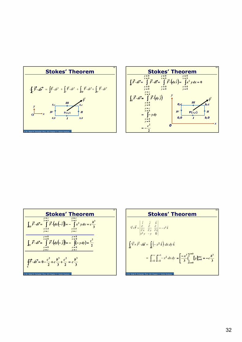
32
© Dr. Nidal M. Ershaidat Phys. 201 Chapter 1': Vector Analysis
135
Stokes’ Theorem
IIII
IIIIII
P(x,y)
II
x
y
OIVIV
→F
∫∫∫∫→→→→→→→→
⋅⋅⋅⋅C
drF ∫ →→⋅+
IIIdrF∫ →→
⋅+II
drF∫ →→⋅=
IdrF ∫ →→
⋅+V
drI
F
0,0 b,0
b,c0,c
136
(((( )))) 0ˆ
0
00
2
0
00
0
00
========⋅⋅⋅⋅====⋅⋅⋅⋅====⋅⋅⋅⋅ ∫∫∫∫∫∫∫∫∫∫∫∫∫∫∫∫========
========
========
========
→→→→========
========
→→→→→→→→→→→→→→→→bx
y
yx
bxy
yx
bxy
yx
IdxyxidxFdlFdrF
Stokes’ Theorem
IIII
IIIIII
P(x,y)
II
x
y
0
IVIV
→F
0,0 b,0
b,c0,c
(((( ))))
2
ˆ
2
0
0
c
dyy
jdyFdrF
bxcy
ybx
bxcy
ybx
II
−−−−====
−−−−====
⋅⋅⋅⋅====⋅⋅⋅⋅
∫∫∫∫
∫∫∫∫∫∫∫∫
========
========
========
========
→→→→→→→→→→→→
© Dr. Nidal M. Ershaidat Phys. 201 Chapter 1': Vector Analysis
137
Stokes’ Theorem
(((( ))))(((( ))))3
ˆ3
2
00bcdxyxidxFdrF
xcy
cybx
xcy
cybx
III====−−−−====−−−−⋅⋅⋅⋅====⋅⋅⋅⋅ ∫∫∫∫∫∫∫∫∫∫∫∫
========
========
========
========
→→→→→→→→→→→→
(((( ))))(((( )))) (((( ))))2
ˆ20
0
0
00
0
cdyyjdyFdrF
xy
cyx
xy
cyx
IV====−−−−−−−−====−−−−⋅⋅⋅⋅====⋅⋅⋅⋅ ∫∫∫∫∫∫∫∫∫∫∫∫
========
========
========
========
→→→→→→→→→→→→
32320
3232 bc
cbc
cdr
C
====++++++++−−−−====⋅⋅⋅⋅∫∫∫∫→→→→→→→→
F
© Dr. Nidal M. Ershaidat Phys. 201 Chapter 1': Vector Analysis
138
Stokes’ Theorem
kx
yyx
yx
kji
ˆ
ˆˆˆ
2
2 0
F −=
−∂∂
∂∂
∂∂
=×∇→→
z
( )∫∫ ⋅−=⋅×∇ →→→
SSa kdydxkxdF ˆˆ2
∫ ∫=
=
=
=−=
cy
y
bx
xdydxx
0 0
2 [[[[ ]]]]33
3
0
0
3bcy
x cy
y
bx
x
−−−−====
−−−−==== ====
====
====
====

33
Potential Theorem
© Dr. Nidal M. Ershaidat Phys. 201 Chapter 1': Vector Analysis
141
Given the force
Problem 1. 61
( ) ( ) ( )kzyxjxyzxiyzyxF 2322223 ++−+−=
→
Solution: This force is conservative if and
only if
z
z
FFF
yx
kji
yx
∂∂
∂∂
∂∂
=×∇→→
ˆˆˆ
F
0FFFFFF
=
∂∂
−∂
∂+
∂
∂−
∂∂
+
∂
∂−
∂∂
= kyx
jx
iy
xyxyz ˆˆˆ z
zz
a) Show that this force is conservative
© Dr. Nidal M. Ershaidat Phys. 201 Chapter 1': Vector Analysis
142
Problem 1. 61
( ) 222 xzyx
yy
Fz =+∂∂
=∂∂ ( ) 222
3 xxyzxzz
Fy =−∂∂
=∂
∂,
( ) yxyzyxzz
Fx22
3 =−∂∂
=∂∂ ( ) yxzyx
xx
Fz22
2 =+∂∂
=∂∂
,
( ) 222323 yzxxyzx
xx
Fy −=−∂∂
=∂
∂
( ) 23322 yzxyzyx
yy
Fx −=−∂∂
=∂∂
0=×∇⇒→→F
© Dr. Nidal M. Ershaidat Phys. 201 Chapter 1': Vector Analysis
143
⇒⇒⇒⇒
b) Find a potential φφφφ(x,y,z) such that
Problem 1. 61 (b)
φ∇−=→→
F
Solution:
φ−=
∂φ∂
+∂
φ∂+
∂φ∂
−=→
→
rd
dkj
yix
ˆˆˆ
zF
32 yxyx +−=φ z 32 yxyx +− z 2zz −− yx2
23223 zyxzyx −+−=φ
∫→→
⋅−=φ rdF ( )dyxyzx∫ −− 223
( )dzzyx∫ +− 22
( )dxyzyx∫ −−= 32


![1 Engineering Economy [1-2] Introduction Examples and Additional Concepts Eng. Nidal Y. Dwaikat.](https://static.fdocuments.in/doc/165x107/56649e395503460f94b2b70b/1-engineering-economy-1-2-introduction-examples-and-additional-concepts-eng.jpg)