Analysis 1 Analysis 1 - · PDF fileAnalysis 1 Analysis 1. ... African Virtual University I....

Prepared by Jairus M. KHALAGAI

African Virtual universityUniversité Virtuelle AfricaineUniversidade Virtual Africana

Analysis 1 Analysis 1

African Virtual University �

Notice

This document is published under the conditions of the Creative Commons http://en.wikipedia.org/wiki/Creative_Commons Attribution http://creativecommons.org/licenses/by/2.5/ License (abbreviated “cc-by”), Version 2.5.


I. Analysis1________________________________________________ 3

II. PrerequisiteCourseorKnowledge_____________________________ 3

III. Time____________________________________________________ 3

IV. Materials_________________________________________________ 3

V. ModuleRationale __________________________________________ 3

VI. Content__________________________________________________ 4

6.1 Overview___________________________________________ 4 6.2 Outline_____________________________________________ 4 6.3 GraphicOrganizer_____________________________________ 6

VII. GeneralObjective(s)________________________________________ 7

VIII. TeachingandLearningActivities_______________________________ 8

IX. LearningActivities_________________________________________ 11

X. GlossaryofKeyConcepts___________________________________ 40

XI. ListofCompulsoryReadings________________________________ 46

XII. CompiledListof(Optional)MultimediaResources________________ 47

XIII. SynthesisoftheModule____________________________________ 48

XIV. SummativeEvaluation______________________________________ 49

XV. References ______________________________________________ 59

XVI.MainAuthoroftheModule__________________________________ 59

Table of ConTenTs


I. analysis 1by Prof. Jairus M. Khalagai

ii. Prerequisite Courses or KnowledgeUnit 1 : Analysis of the real line

Basic mathematics and calculus

Unit 2 : Vector Analysis

Calculus

Unit 3 : Complex Analysis

Calculus and Analysis unit 1

III. TimeThe total time for this module is 120 study hours.

IV. MaterialStudents should have access to the core readings specified later. Also, they will need a computer to gain full access to the core readings. Additionally, students should be able to install the computer software wxMaxima and use it to practice algebraic concepts.

V. Module RationaleThe rationale of teaching analysis is to set the minimum content of Pure Mathematics required at undergraduate level for student of mathematics. It is important to note that skill in proving mathematical statements is one aspect that learners of Mathematics should acquire. The ability to give a complete and clear proof of a theorem is essential for the learner so that he or she can finally get to full details and rigor of analyzing mathematical concepts. Indeed it is in Analysis that the learner is given the exposition of subject matter as well as the techniques of proof equally. We also note here that if a course like calculus with its wide applications in Mathematical sciences is an end in itself then Analysis is the means by which we get to that end.


VI. Content

6.1 Overview

This module consists of three units which are as follows:

Unit 1 - Analysis on the real line

In this unit we start by decomposing the set ° of real numbers into its subsets. We then define the so called standard metric on ° to be able to study its structure which consists of concepts like open and closed intervals, neighbourhoods, interior and limit points leading to examples of open and closed subsets of ° . Countability of such subsets and numerical sequences are also essential in the structure of ° as a metric space. We also study functions defined on sets of real numbers with respect to concepts of continuity differentiability and integrability.

Unit 2 – Vector Analysis

This unit deals with mainly vector calculus and its applications. Thus we specifi-cally consider concepts like gradient, divergence and curl. This leads to well known theorems like Green’s stokes divergence theorems and other related results. The curvilinear coordinates system is also given a treat in this unit.

Unit 3 – Complex Analysis

The main objective in the study of this unit is to define a function of a complex va-riable and then look at its degree of smoothness such as existence of limit, continuity and differentiability along the lines of calculus of functions of a real variable. Also a look at integration and power series involving a function of a complex variable will complete this unit.

6.2 Outline: Syllabus

Unit 1a – Introduction to Analysis (25 hours)

Level priority Basic Mathematics and Calculus are Pre-requisites

• Real number system and completeness• Open, closed intervals and neighbourhoods• Interior points, limit points• Uncountability of the real line• Sequences• Functions, limits and continuity• Differentiability and integrability


Unit 1a – The Riemann Integral (15 hours)

• Define the Riemann integral

• Give examples of Riemann integrals defined on the set ° .• State some properties of a Riemann integral• Verify or prove some results on Riemann integrals.

Unit 2 – Vector Analysis (40 hours)

Level priority Basic Mathematics and Calculus are Pre-requisites

• Gradient, divergence and Curl• Green’s, Stokes and divergence theorems• Other related theorems• Curvilinear coordinates

Unit 3 – Complex Analysis (40 hours)

Level priority Unit 1 is the Pre-requisite

• Definition and examples of a complex variable• Limits, continuity and differentiability• Analytic functions• Complex integration• Power and Laurent series


6.3 Graphic Organiser

Module Development Template 4

Graphic Organiser

Limits, continuity and

differentiability

Vector Calculus and Applications

Riemann Integrals

Functions of a real

variable

Structure of the space

Vector valued functions

Structure of a vector space

Space Structure of the complex number field

Functions of a complex

variable limits and continuity

Analytic functions, power

series and Laurent series

Complex integration


VII. specific learning objectives (Instructional objectives)

You should be able to:

1. Demonstrate understanding of basic concepts and principles of mathematical analysis.

2. Develop a logical framework for stating and proving theorems.


VIII. Teaching and learning activities

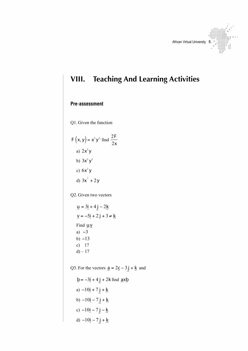
Pre-assessment

Q1. Given the function

F x, y( ) = x3 y2 , find

2F2x

a) 2x3 y

b) 3x2 y2

c) 6x2 y

d) 3x2

+ 2 y

Q2. Given two vectors

u = 3i + 4 j − 2k

v = −5i + 2 j + 3 ≠ k

Find u.va) −3b) −13c) 17d) – 17

Q3. For the vectors a = 2c − 3 j + k and

b= −3i + 4 j + 2k find axb

a) −10i + 7 j + k

b) −10i − 7 j + k

c) −10i − 7 j − k

d) −10i − 7 j + k


Q4. Given the complex numbers

Z = 3+ 4i and Z2= −2 + 3i

find Z1+ Z

2

a) 150 b) 24 c) 5 d) 38

Q5. Given two complex numbers

Z1= 5+ 2i and Z2

= 4 + 3i

find Arg Z1Z

2

a) tan

−1 2

5 b) tan

− 23

14 c) tan

−13

4 d) tan

−15

9

Q6. Evaluate

1+ 2i3− 4i

+2 − i5i

a)

−2

5 b)

5

2 c) 1 d)

3+ i3− i

Q7. Express the complex number

Z=1+I in modulus argument form

a) Z=

3 cos

+∏4

i sin∏4

⎛

⎝⎜

⎞

⎠⎟

b) Z=

2 cos∏

3+ Sin∏

3

⎛

⎝⎜

⎞

⎠⎟

c) Z

= 2 cos∏

4+ iSin∏

4

⎛

⎝⎜

⎞

⎠⎟ d) Z=

3 cos∏

3+ iSin∏

3

⎛

⎝⎜

⎞

⎠⎟

African Virtual University �0

Q.8 Which of the following functions is not continuous at x = o?

a)

x( ) = x2∫ b) g

x( ) = 1+ x2

c) h

x( ) = x d) None

Q9. Which of these functions is not different at x = o?

a)

x∫ = x2 b) g x( ) = 1+ x2

c) h x( ) = x

h x( ) = x d) None

Q10. Which one of the following statements is true about the number 2

a) yf is an integerb) It is a fractionc) It is a rationald) It is irrational

Pre-assessment: Solutions

Q 1. (b)Q 2. (b)Q 3. (c)Q 4. (a)Q 5. (b)Q 6. (a) Q 7. (c)Q 8. (d)

Q 7. (c)

African Virtual University ��

IX. learning activities

Analysis 1: Unit 1a

Title: Introduction to Analysis

Specific Objectives

At the end of this activity the learner will be able to:

• Decompose the set ℜ of real numbers into various subsets.• State properties of various subsets of ℜ.• Define the concept of boundedness of sets of real numbers.• State and use the completeness axiom to solve problems on real number sys-

tem.

Summary

We first note that a satisfactory discussion of the main concepts of Analysis (e.g. convergence, continuity, differentiability and integration), must be based on an accurately defined number concept. To this end the real number system is indeed a well defined concept. It is clear here that the axioms governing the arithmetic of the integers are well known and trivial at this level. However, we need to familiarize

ourselves with the arithmetic of rational numbers (i.e. numbers of the form

nm

where

n and m are integers m≠ 0) and we shall list the main feature of the arithmetic of

such numbers as that of being closed under both addition and multiplication.

We also note that a relation < is defined and brings order on the set of rational numbers.

Thus for any two rational numbers p and q we have that either p = q or q < p and it is transitive. It is also known that the rational number system is inadequate. For

instance there is no rational number p such that p2 = 2 .

This leads to the introduction of the set of irrational numbers. Thus the union of the set of rational numbers and the set of irrational numbers constitutes the set ° of real numbers. We will also consider the concept of a set of real numbers being bounded below or above. This leads to the completeness axiom that characterizes the set ° of real numbers completely.


Key Concepts

• Rational number: This is a number that can be written in the form

nm

where n and m are integers with m≠ 0 and 1 as the only common factor for n and m.

• Irrational number: This is a number that cannot be written in the form

nm

, where n and m are integers with m≠ 0 . Thus, we have that the set of rational

numbers is § and the set of irrational numbers §C leading to the relation

° = § ∪§ C

i.e. Every real number is either rational or irrational• Bounded below: Any set E of real numbers is said to be bounded below if

there is a real number q such that q ≤ x ∀ x∈E. In this case q is called a lower bound for E.

• Bounded above: Any set E of real numbers is said to be bounded above if

there is a real number p such that p ≥ x ∀ x∈E. In this case p is called an upper bound for E.

• Infimum: For any set E of real numbers, the largest of all real numbers q

such that q ≤ x ∀ x∈E. is called infimum of E written Inf E or is called greatest lower bound written glb E.

• Supremum: For any set E of real numbers the smallest of all real numbers

p such that p ≥ x ∀ x∈E is called the supremum of E written sup E or is called the least upper bound of E written lub E.

• Completeness axiom: This states as follows: Every non empty set E of real numbers bounded above has supremum and if bounded below has infimum.


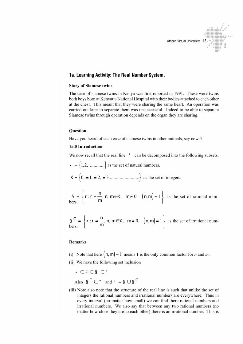
1a. Learning Activity: The Real Number System.

Story of Siamese twins

The case of siamese twins in Kenya was first reported in 1991. These were twins both boys born at Kenyatta National Hospital with their bodies attached to each other at the chest. This meant that they were sharing the same heart. An operation was carried out later to separate them was unsuccessful. Indeed to be able to separate Siamese twins through operation depends on the organ they are sharing.

Question

Have you heard of such case of siamese twins in other animals, say cows?

1a.0 Introduction

We now recall that the real line ° can be decomposed into the following subsets.

• = 1,2, ............{ } as the set of natural numbers.

¢ = 0, ±1, ± 2, ± 3,........................{ }

as the set of integers.

§ = r : r =

nm

, n, m∈¢ , m≠ 0, n,m( ) = 1⎧⎨⎩

⎫⎬⎭

as the set of rational num-bers.

§ C = r : r ≠

nm

, n, m∈¢ , m≠ 0, n,m( ) = 1⎧⎨⎩

⎫⎬⎭

as the set of irrational num-bers.

Remarks

(i) Note that here

n,m( ) = 1 means 1 is the only common factor for n and m.

(ii) We have the following set inclusion

• ⊂ ¢ ⊂ § ⊂ °

Also §C ⊂ ° and ° = § ∪ § C

(iii) Note also note that the structure of the real line is such that unlike the set of integers the rational numbers and irrational numbers are everywhere. Thus in every interval (no matter how small) we can find there rational numbers and irrational numbers. We also say that between any two rational numbers (no matter how close they are to each other) there is an irrational number. This is


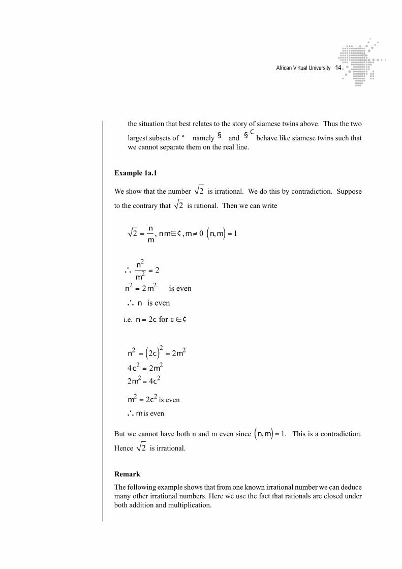
the situation that best relates to the story of siamese twins above. Thus the two

largest subsets of ° namely § and §C

behave like siamese twins such that we cannot separate them on the real line.

Example 1a.1

We show that the number 2 is irrational. We do this by contradiction. Suppose

to the contrary that 2 is rational. Then we can write

2 =nm

, nm∈¢ ,m≠ 0 n,m( ) = 1

∴ n2

m2 = 2

n2 = 2 m2 is even

∴ n is even

i.e. n = 2c for c ∈¢

n2 = 2c( )2 = 2m2

4c2 = 2m2

2m2= 4c2

m2 = 2c2 is even

∴mis even

But we cannot have both n and m even since

n,m( ) = 1. This is a contradiction.

Hence 2 is irrational.

Remark

The following example shows that from one known irrational number we can deduce many other irrational numbers. Here we use the fact that rationals are closed under both addition and multiplication.


Example 1a.2

Let t be an irrational number. Show that

t +1

t − 1is also irrational.

Solution

Let s =

t +1

t − 1 and assume to the contrary that s is rational. Then we have

s t − 1( ) = t +1

st − s = t +1

st − t = 1+ s

t s −1( ) = s +1

t =s +1

s −1

Since rationals are close under multiplication and addition we have that:

s+ ts −1

is also rational.

But t is irrational. This is a contradiction. Hence

t +1

t −1 is also irrational.

Exercise 1a.3

(i) Given that a and b are rational numbers and s is irrational show that a − bs is also irrational.

(ii) Given that for p prime p is irrational show that:

3 +1

3 −1is irrational.


Example 1a.4

Let E ⊆ ° be given by E = x ∈ ° : 1 < x ≤ 5{ } . Then E is bounded below and

above. In this case inf E = 1 and sup E = 5 .

Note that if inf E ∈E then inf E is called minimum element of E written

min E. Also if sup E∈E then sup E is called the maximum element of E written

max E.

In the example above inf E =1∉E and thus E has no minimum element. But

sup E =5∈E and thus E has the maximum element which is 5.

Exercise 1a.5

(i) Let E be a bounded set of real numbers such that a = inf E and b = max E. Give the definitions of a and b. Also give an example of a set where both a and b exist.

(ii) Let

S =

1

n; n∈J +⎧

⎨⎩

⎫⎬⎭

Thus

S = 1,

1

2,

1

3,

1

4, ................

⎧⎨⎩

⎫⎬⎭

.

State sup S, inf S. max S and min S.

1a.6. Readings

1. Read the following sections from Elias Zakon, Basic Concepts in Maths, Trillia Press.

Part 1, chapters 8 and 9.Part 2, chapters 1, 2, 3, 4, 5, 6, 7, 8, 9, and 10.

Complete and check all of the exercises in these sections.

2. Read the Wikipedia reference: Reimann Integrals.

For updates and links search for ‘Reimann Integrals’ at www.wikipedia.org


Analysis 1 Module: Unit 1b

Title: The Riemann Integral

Specific Objectives


• Define the Riemann integral

• Give examples of Riemann integrals defined on the set ° .• State some properties of a Riemann integral• Verify or prove some results on Riemann integrals.

Summary

In this activity we formulate the Riemann integral which depends explicitly on the order structure of the real line. Accordingly we begin by discussing the concept of a partition of an interval and show that formulation of the Riemann integral is es-sentially one of the methods of estimating area under a given curve. Indeed it is the most accurate method of finding area bounded by a given curve. We thus define the relevant concepts like lower and upper sums that lead to lower and upper Riemann integrals respectively before we derive the actual Riemann integral.

We will also discuss briefly properties and classes of real valued functions which are Riemann integrable and give at least one example of a function which is not Riemann integrable. The extension of this theory to complex and vector valued functions on intervals and over sets other than intervals is subject matter of higher courses that can be discussed at graduate level.

Key Words and Concepts

• Partition of an interval: Let

a,b⎡⎣ ⎤⎦ be an interval in ° and let

x0 , x1,.........., xn be such that a = x0 < x1 < x2 < ......... < xn = b . Then the

set P = x0 , x1,.........., xn{ } is called a partition of

a, b⎡⎣ ⎤⎦ and the class of

all partitions of

a, b⎡⎣ ⎤⎦ is denoted by Ρ a, b⎡⎣ ⎤⎦ .

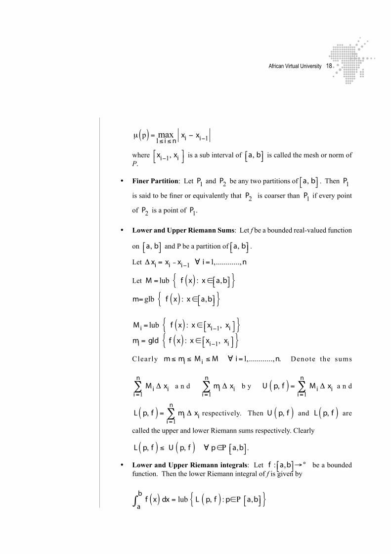
• Mesh of a partition: let P be a partition of

a, b⎡⎣ ⎤⎦ . Then the number denoted

by μ p( ) given by


μ p( ) = max

1≤ i ≤nxi − xi−1

where

xi−1, xi⎡⎣

⎤⎦ is a sub interval of

a, b⎡⎣ ⎤⎦ is called the mesh or norm of

P.

• Finer Partition: Let P1 and

P2 be any two partitions of

a, b⎡⎣ ⎤⎦ . Then P1

is said to be finer or equivalently that P2 is coarser than

P1 if every point

of P2 is a point of

P1.

• Lower and Upper Riemann Sums: Let f be a bounded real-valued function

on

a, b⎡⎣ ⎤⎦ and P be a partition of

a, b⎡⎣ ⎤⎦ .

Let Δ xi = xi − xi−1 ∀ i=1,............,n

Let M = lub f x( ) : x ∈ a,b⎡⎣ ⎤⎦{ }

m=glb f x( ) : x ∈ a,b⎡⎣ ⎤⎦{ }

Mi = lub f x( ) : x ∈ xi−1, xi⎡⎣ ⎤⎦{ }mi = gld f x( ) : x ∈ xi−1, xi⎡⎣ ⎤⎦{ }

Clear ly m≤ mi ≤ Mi ≤ M ∀ i=1,............,n. Denote the sums

Mi Δ xi

i=1

n

∑ a n d

mi Δ xi

i=1

n

∑ b y

U p, f( ) = Mi Δ xi

i=1

n

∑ a n d

L p, f( ) = mi Δ xi

i=1

n

∑ respectively. Then U p, f( ) and

L p, f( ) are

called the upper and lower Riemann sums respectively. Clearly

L p, f( ) ≤ U p, f( ) ∀ p∈Ρ a,b⎡⎣ ⎤⎦.

• Lower and Upper Riemann integrals: Let f : a,b⎡⎣ ⎤⎦→ ° be a bounded

function. Then the lower Riemann integral of f is given by

f x( ) dx

a

b∫ = lub L p, f( ) : p∈Ρ a,b⎡⎣ ⎤⎦{ }


and the upper Riemann integral of f is given by

f x( ) dxa

b∫ = glb U p, f( ) : p∈Ρ a,b⎡⎣ ⎤⎦{ }

• Riemann integral of a function: Let f : a,b⎡⎣ ⎤⎦→ ° be a bounded real-valued

function. Then f is said to be Riemann integrable if

f x( ) dx

a

b∫ = f x( ) dx

a

b∫ = f x( ) dx

a

b∫ .

In this case the common value

f x( ) dxa

b∫ is called the Riemann integral

of the function f.

1b Introduction The Story of Fred the Mathematical Fly

It is a common practice in our African culture that people tell stories or cite legends by referring to either animals or even insects when the message carried in such stories refer to behaviour of human beings. To this end our current story of modern times concerns Fred the mathematical fly who one day was moving on a curve whose equation was known.

He gave an assignment to his friends who were watching him as he moves on the given curve as follows:

Describe for me the procedure with which I can find my speed at any point on this curve. Also tell me the procedure to find most accurately the area bounded by this curve with respect to the two axes.

Picture showing a fly moving on a curve

curve fly


Question

What are your answers to the two questions posed by Fred the mathematical fly in the story above?

1b.1 Introduction

We note that in the story above the two questions posed by the mathematical fly are addressing both theories of differential and integral calculus. Indeed we will show by the way of stating a theorem that differentiation and integration are in a way inverse operations.

We also note that from the definitions of lower and upper Riemann sums that clearly the formulation of the Riemann integral is based on estimating area under a given curve. Note that as we make the partition finer the lower Riemann sum increases to the actual area and the upper Riemann sum decreases to the actual area. Thus by taking the least upper bound of lower sums and the greatest lower bound of the upper sums we get a common value that becomes the Riemann integral.

Remark 1b.1

The example below shows that there are real-valued functions which are not Riemann integrable.

Example 1b.2.

Let f : a,b⎡⎣ ⎤⎦→ ° be a function defined by

f x( ) = 1 if x is rational

0 if x is irrational

⎧⎨⎩

Let P be any partition of

a,b⎡⎣ ⎤⎦. Then in any of the subintervals

xi−1 , xi⎡⎣

⎤⎦ ∀ i = 1,........,n.

we have:

Mi = lub f x( ) :x ∈ xi−1 , xi⎡⎣

⎤⎦{ } = 1

mi = glb f x( ) :x ∈ xi−1 , xi⎡⎣

⎤⎦{ } = 0


Thus

U p, f( ) = Mi Δ xii =1

n∑

= 1 Δ xii =1

n∑

= 1 b− a( )= b− a > 0

and

L p, f( ) = mi Δ xii =1

n∑

= 0 Δ xii =1

n∑

= 0

∴glb U p, f( ) : p∈ρ a,b⎡⎣ ⎤⎦{ }= 1 = f dxa

b∫

lub L p, f( ) : p∈ρ a,b⎡⎣ ⎤⎦{ }= 0= f dxa

b∫

Thus

f dx

a

b∫ = 0 ≠ 1= f dx

a

b∫

Hence f so defined above is not Riemann integrable.

Remark 1b.3

We state without proofs some of the theorems that give properties and classes of Riemann integrable functions.

Theorem 1b.4 (Criterion for Riemann integrability)

Let f be bounded on

a,b⎡⎣ ⎤⎦ . Then f is Riemann integrable iff for each

ε > 0 ∃ p∈P a,b⎡⎣ ⎤⎦


such that

U p, f( ) − L p, f( ) < ε

Theorem 1b.5

Let f be bounded on

a,b⎡⎣ ⎤⎦. If f is monotonic on

a,b⎡⎣ ⎤⎦ then f is Riemann inegrable.

Theorem 1b.6

Let f be bounded on

a,b⎡⎣ ⎤⎦ . If f is continuous, then f is Riemann integrable.

Example 1b.7

Consider the function

f : 0,

π

2

⎛

⎝⎜⎤

⎦⎥→ ° given by

f x( ) = sin2 x

We note that f is continuous on

0,

π

2

⎛

⎝⎜⎤

⎦⎥ and hence Riemann integrable on

0,

π

2

⎛

⎝⎜⎤

⎦⎥.

Indeed

sin2 x dx =0

π2∫

1

2−

1

2cos2x

⎛

⎝⎜⎞

⎠⎟dx

0

π2∫

=1

2x

π

2−

1

4sin π

⎛

⎝⎜⎞

⎠⎟− 0

=π

4−0 =

π

4


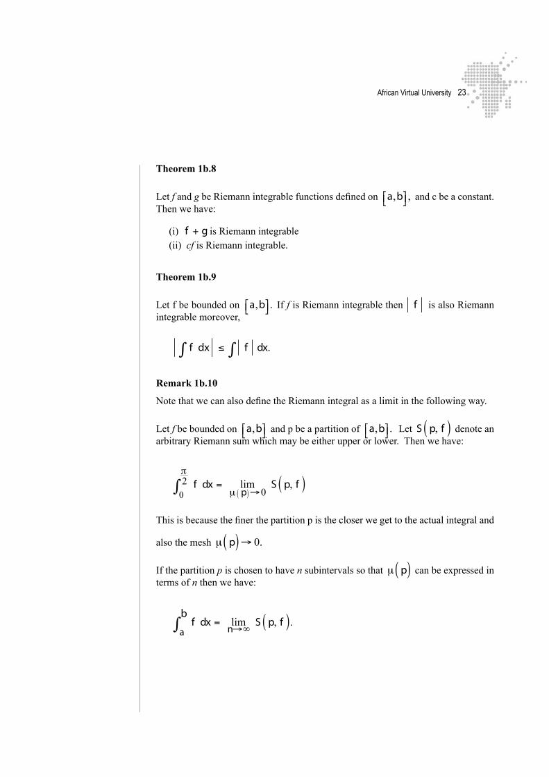
Theorem 1b.8

Let f and g be Riemann integrable functions defined on

a,b⎡⎣ ⎤⎦ , and c be a constant. Then we have:

(i) f + g is Riemann integrable (ii) cf is Riemann integrable.

Theorem 1b.9

Let f be bounded on

a,b⎡⎣ ⎤⎦. If f is Riemann integrable then

f is also Riemann integrable moreover,

f d∫ x ≤ f∫ dx.

Remark 1b.10

Note that we can also define the Riemann integral as a limit in the following way.

Let f be bounded on

a,b⎡⎣ ⎤⎦ and p be a partition of

a,b⎡⎣ ⎤⎦. Let S p, f( ) denote an

arbitrary Riemann sum which may be either upper or lower. Then we have:

f dx =0

π2∫ lim

μ p( )→0S p, f( )

This is because the finer the partition p is the closer we get to the actual integral and

also the mesh μ p( )→ 0.

If the partition p is chosen to have n subintervals so that μ p( ) can be expressed in

terms of n then we have:

f dx =a

b∫ lim

n→∞S p, f( ).


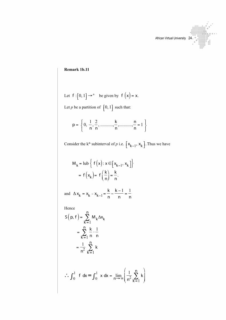
Remark 1b.11

Let f : 0, 1⎡⎣ ⎤⎦→ ° be given by

f x( ) = x.

Let p be a partition of

0, 1⎡⎣ ⎤⎦ such that:

p = 0,

1

n,

2

n, ...........,

kn

,...........,nn= 1

⎧⎨⎩

⎫⎬⎭

Consider the kth subinterval of p i.e.

xk−1, xk⎡⎣ ⎤⎦.Thus we have

M k = lub f x( ) : x ∈ xk−1, xk⎡⎣ ⎤⎦{ }= f xk( )= f

kn

⎛

⎝⎜⎞

⎠⎟=

kn

.

and Δ xk = xk − xk−1=

kn−

k −1

n=

1

n

Hence

S p, f( ) = M kk =1

n∑ Δxk

=kn⋅

1

nk =1

n∑

=1

n2 kk =1

n∑

∴ f dx0

1∫ = x dx = lim

n→∞1

n2 kk =1

n∑

⎛

⎝⎜⎜

⎞

⎠⎟⎟0

1∫


Exercise 1b.12

(i) Show that the function defined by

f x( ) = 2 if x is rational

−2 if x is irrational

⎧⎨⎩

is not Riemann integrable.

(ii) Consider the function f : 0, a⎡⎣ ⎤⎦→ ° given by

f x( ) = x3 where a is a

constant. Show that

x

3dx

0

a∫ = lim

n→∞a4

n4 k3

k = 1

n

∑⎛

⎝⎜

⎞

⎠⎟

(iii) Given

π

nsin

knπ

k = 1

n

∑ as a Riemann sum, use this fact to evaluate

lim

n→∞π

nsin

knπ

k = 1

n

∑⎛

⎝⎜

⎞

⎠⎟

Readings

1. Theory of functions of a real variable by - Shilomo Stenberg (2005) pp 1442. Read the Wilkipedia reference: Riemann Integrals.

For updates and links search for ‘Riemann Integrals’ at www.wikipedia.org


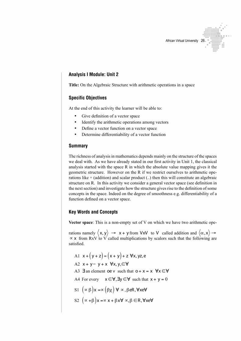
Analysis I Module: Unit 2

Title: On the Algebraic Structure with arithmetic operations in a space

Specific Objectives


• Give definition of a vector space• Identify the arithmetic operations among vectors• Define a vector function on a vector space• Determine differentiability of a vector function

Summary

The richness of analysis in mathematics depends mainly on the structure of the spaces we deal with. As we have already stated in our first activity in Unit 1, the classical analysis started with the space R in which the absolute value mapping gives it the geometric structure. However on the R if we restrict ourselves to arithmetic ope-rations like + (addition) and scalar product (..) then this will constitute an algebraic structure on R. In this activity we consider a general vector space (see definition in the next section) and investigate how the structure gives rise to the definition of some concepts in the space. Indeed on the degree of smoothness e.g. differentiability of a function defined on a vector space.

Key Words and Concepts

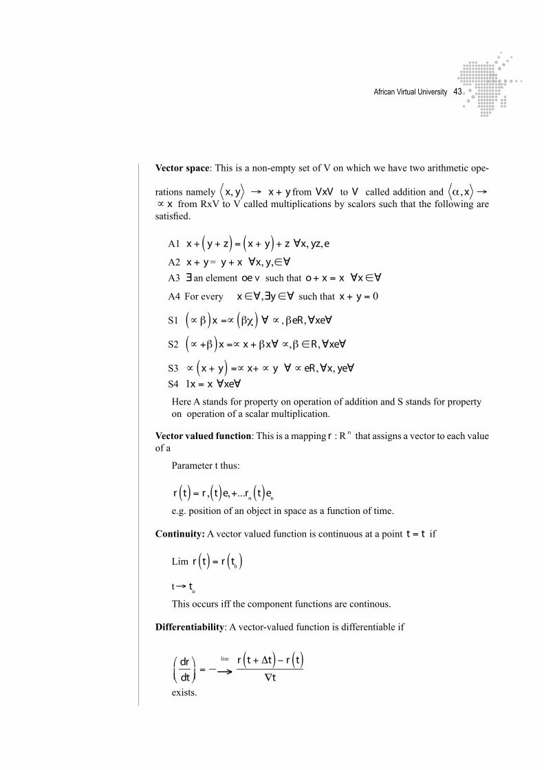
Vector space: This is a non-empty set of V on which we have two arithmetic ope-

rations namely

x, y → x + y from VxV to V called addition and α , x →

∝ x from RxV to V called multiplications by scalors such that the following are satisfied.

A1 x + y + z( ) = x + y( ) + z ∀x, yz,e

A2 x + y = y + x ∀x, y,∈∀

A3 ∃ an element oe∨ such that o+ x = x ∀x ∈∀

A4 For every x ∈∀,∃y ∈∀ such that x + y = 0

S1 ∝ β( )x =∝ βχ( ) ∀ ∝ , βeR ,∀xe∀

S2 ∝ +β( )x =∝ x + βx∀ ∝,β ∈R ,∀xe∀


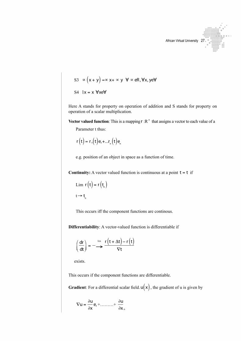
S3 ∝

x + y( ) =∝ x+ ∝ y ∀ ∝ eR ,∀x, ye∀

S4 1x = x ∀xe∀

Here A stands for property on operation of addition and S stands for property on operation of a scalar multiplication.

Vector valued function: This is a mapping r :R n that assigns a vector to each value of a

Parameter t thus:

r t( ) = r , t( )e,+...r

nt( )e

n

e.g. position of an object in space as a function of time.

Continuity: A vector valued function is continuous at a point t = t if

Lim r t( ) = r t

0( ) t → t

o

This occurs iff the component functions are continous.

Differentiability: A vector-valued function is differentiable if

drdt

⎛

⎝⎜⎞

⎠⎟=

lim

→

r t + Δt( ) − r t( )∇t

exists.

This occurs if the component functions are differentiable.

Gradient: For a differential scalar field. u x( ) , the gradient of u is given by

∇u =

∂u∂x

e, +………+

∂u∂x n


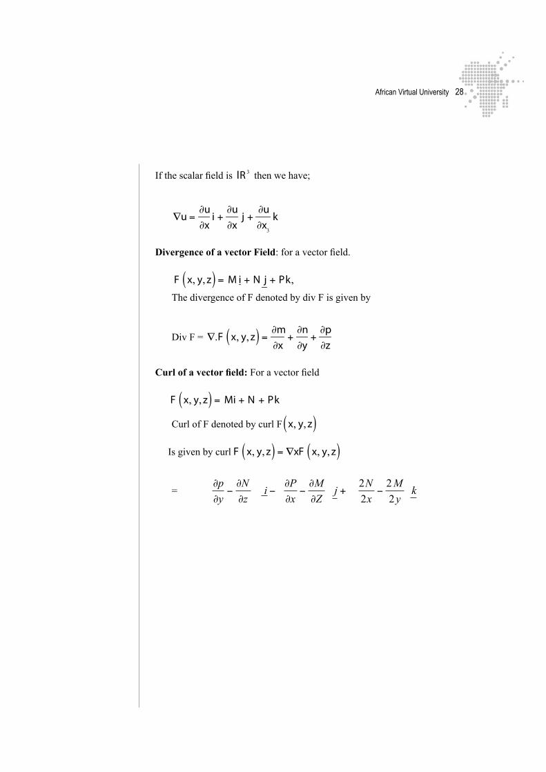
If the scalar field is lR3 then we have;

∇u =

∂u∂x

i +∂u∂x

j +∂u∂x

3

k

Divergence of a vector Field: for a vector field.

F x, y, z( ) = M i + N j + Pk,

The divergence of F denoted by div F is given by

Div F = ∇.F x, y, z( ) = ∂m

∂x+∂n∂y

+∂p∂z

Curl of a vector field: For a vector field

F x, y, z( ) = Mi + N + Pk

Curl of F denoted by curl F

x, y, z( )

Is given by curl F x, y, z( ) = ∇xF x, y, z( )

= ∂

∂−∂

∂

p

y

N

z

iP

x

M

Zj−

∂

∂−∂

∂+

2

2

2

2

N

x

M

yk−


2. On the Algebraic Structure with arithmetic operations in a space

Story of Investigation in Gender Issues

In the year 2006 some time in October an N.G.O. dealing with gender issues in the city of Nairobi dispatched an agent to some premises of a business company. The company had just been started and the N.G.O. was eager to find out whether women also have some initiative to deal with the company. The task of this agent called Mwangi was to count the number of women in a random turnover on the premises within some specified time. While in the premises he stood at a point where people were passing to various directions. Some of them in groups so large that they could even push her out of the way and in the process she loses the count.

Question

Could you suggest a better way or better point where Mwangi should have stood to have an accurate count?

2.0 Introduction

We note that in the story above rather than standing at a corner from where people are passing to all directions the agent should have used a point like the entrance or exit where movement is in only one particular direction. This is the main reason why we consider vector-valued functions because they create motion in a specific direction. Consequently the components of vector calculus like divergence and curl have applications in diverse fields like electromagnetism, fluid mechanism, etc.

We note that if the vector valued function vt, represents the position of a moving ob-

ject then

ddt

and

d2

dt2 are also vector valued functions representing velocity

and acceleration respectively.

Example 2.1

Consider the parametric curve:

r (t) = cos

t2

i + sint2

j−

Find velocity and acceleration vectors.

Find velocity and acceleration vectors.


Solution

Velocity =

drdt

=1

2sin

t2

i +1

2cos

t2

j

Acceleration = d2 vdt2 =

−14

cos t2

i−−

14

sin t2

j−

Exercise 2.2

Let r (t) be the position of an object moving at constant speed. Show that the acceleration of the object is orthogonal to the velocity of the object.

Example 2.3

Given the vector field f (x, y, z) = x3 y2 z i−+ x2 zj + x2 yk find the divergence at

(2,1,−1)

Solution

divF (x, y, z) = 22x

(x3 y2 z) + 22y

(x2 ) + 22z

(x2 y)

= 3x2 y2 z + 0 + 0 = 3x2 y2 z

At the point (2,1,−1)divF = 3x22 x12 x −1= −12

Exercise 2.4

Find the divergence at the point (3,−2,1) for the vector field

F (x, yz) = x2 y3zi + xz2 j + xy2 k

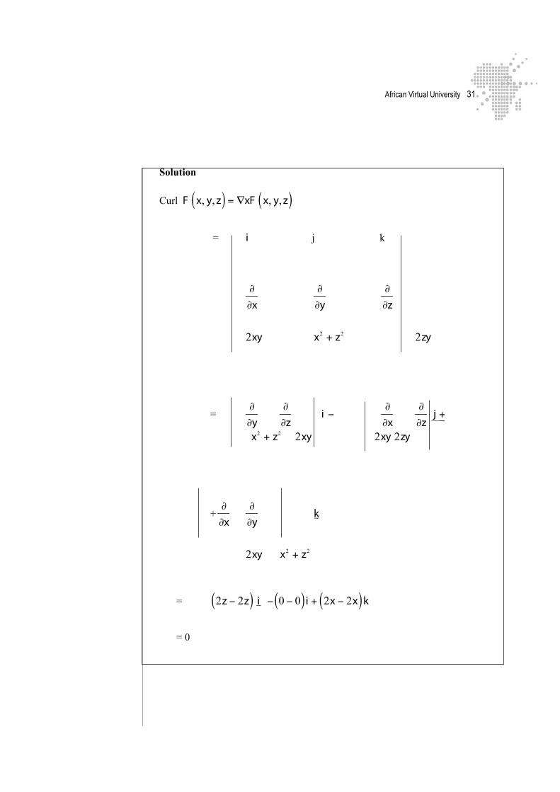
Example 2.5

Find Curl F for the vector field given by

F (x, y, z) = 2xy i−+ (x2 + z2 ) j

−

+ 2zy k−


Solution

Curl F x, y, z( ) = ∇xF x, y, z( )

= i j k

∂

∂x

∂

∂y

∂

∂z

2xy x2 + z2 2zy

=

∂

∂y

∂

∂z i −

∂

∂x

∂

∂z j +u xuu

x2 + z2 2xy 2xy 2zy

+

∂

∂x

∂

∂y

kx

2xy x2 + z2

= 2z − 2z( )

ix − 0 − 0( ) i + 2x − 2x( )k

= 0


Exercise 2.6

a) Given F x, y, z( ) = x2 + y2 − Z

Find ∇F at the point 1,1,2( )

b) Find the divergence at the point −3,2,1( ) for the vector field

F x, y, z( ) = 2xyi + x

2

+ z2( ) j + 2zyk

c) Find the curl at the point −1,2,1( ) for the vector field.

F x, y, z( ) = x3 y2 zi + x

2

yk

Readings

1. Larson Hostetler, Edwards, Calculus with analytic geometry, Houghton Mifflin Company New York 1988.

2. Divergence and Curl (Wikipidia)


Analysis 1: Unit 3

Title: Calculus of functions of complex variables

Specific Objectives


• Define a function of a complex variable;• Give examples of functions of complex variables;• Evaluate limits involving functions of complex variables;• Determine continuity of a function of a complex variable;• Determine differentiability of a function of a complex variable.

Summary

We first note that from the Calculus Module the so called degree of smoothness of a function of a real-variable starts with definition where we have to state the domain and range. We then examine the existence of limit of such a function at some spe-cified point. We also investigate continuity at a given point or on the whole domain followed by differentiability of the function at a point or on the whole domain in this case we have the following implications. Thus

Differentiability => Continuity => Existence of limit.

In this activity we go through the same process for the case of a function of a complex variable. However, it may be of great importance to note that a function f (z) of a complex variable z may also be viewed as a function of two real variables x and ysince z = x + iy where x and y are real variables.

Key Words and Concept

• Function of a complex variable: this is a function whose domain is the set

⊄ of complex number field and range is either ⊄ or R for example f (z) = Z 2

where z = x + iy

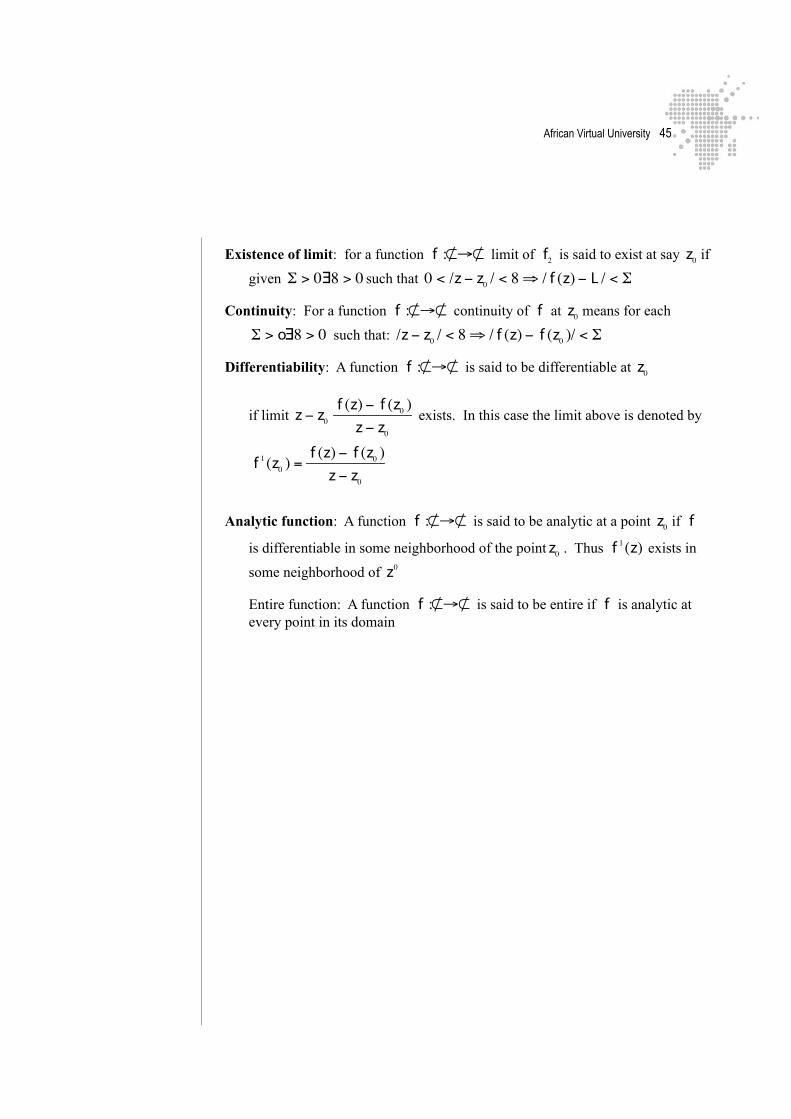
• Existence of limit: for a function f :⊄→⊄ limit of f2 is said to exist at say

z0 if given Σ > 0∃8 > 0 such that 0 < /z − z0 / < 8 ⇒ / f (z) − L / < Σ

• Continuity: For a function f :⊄→⊄ continuity of f at z0 means for each

Σ > o∃8 > 0 such that: /z − z0 / < 8 ⇒ / f (z) − f (z0 )/ < Σ


• Differentiability: A function f :⊄→⊄ is said to be differentiable at z0 if

limit z − z0

f (z) − f (z0 )z − z0

exists. In this case the limit above is denoted by

f 1 (z0 ) = f (z) − f (z0 )z − z0

• Analytic function: A function f :⊄→⊄ is said to be analytic at a point z0 if

f is differentiable in some neighborhood of the point z0 . Thus f 1 (z) exists

in some neighborhood of z0

• Entire function: A function f :⊄→⊄ is said to be entire if f is analytic at every point in its domain.

3 Calculus of functions of complex variables

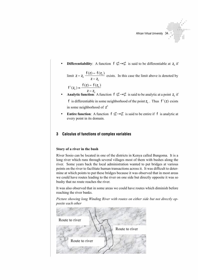
Story of a river in the bush

River Sosio can be located in one of the districts in Kenya called Bungoma. It is a long river which runs through several villages most of them with bushes along the river. Some years back the local administration wanted to put bridges at various points on the river to facilitate human transactions across it. It was difficult to deter-mine at which points to put these bridges because it was observed that in most areas we could have routes leading to the river on one side but directly opposite it was so bushy that no route reaches the river.

It was also observed that in some areas we could have routes which diminish before reaching the river banks.

Picture showing long Winding River with routes on either side but not directly op-posite each other

Route to river

Route to river

Route to river


Question

Can you deduce a condition to be satisfied by the routes on either side of the river so that we determine where to put a bridge?

3.0 Introduction

Recall that in the module of Calculus we came across the concept of continuity of a

function of a real variable in which we saw that a function f : R → R is continuous

at say x0 if the following three conditions are satisfied:

i) f is defined at x0

ii) Limit f (x) exists x → x0

iii) Limit f (x) = f (x0 )x → x0

This situation prevails even in the case of functions of complex variables. Although in our section of key words and concepts we have used E, S definition of continuity we note that this is just an equivalent statement which ensures that the three conditions above are satisfied. The story of the river above says everything about this situation. Indeed we must have routes leading to the river on either side and reaching the river banks directly opposite each other so that a bridge provides continuity of movement across the river and on either side of it. For routes that do not reach the river it means that limit does not even exist for them at the river and therefore, we cannot leave continuity of movement across the river.

Example 3.1

z2 = z

0

2

Remark

The example above shows that in some cases particularly when we are dealing with continuous functions we can evaluate limits in the same way as functions of real va-riables. However, with respect to complex variables a function of a complex variable can be regarded as a function of two real variables. This leads to partial evaluation of limits and also when it comes to differentiability we deal with partial derivatives. We state some theorems below to help this theory to this end.


Theorem 3.2

Let z = x + iy and f be a function of z . Then we can express f into its real and imaginary parts as:

f (z) = u(x, y) + iv(x, y) For a fixed z0 = x0 + iy0 we have limu(x, y0 ) = a =

x → x0

limu(x0 y)y→ y0

And lim v(x, y0 ) = b = lim v(x0 y)x → x0

Remark

Note that the Cauchy-Riemann conditions are only necessary but not sufficient for the derivative to exist. Thus for the converse of the theorem above we require the following result.

Theorem 3.3 (Launch the Riemann condition)

If f (z0 ) exists then

∂u∂x

z0 =∂v∂y

⎛

⎝⎜⎞

⎠⎟2

0 and

2v2x

⎛⎝⎜

⎞⎠⎟Ζ 0 =

2u2y

⎛

⎝⎜⎞

⎠⎟Ζ 0

Also f Ζ 0( ) = 2u2x

⎛⎝⎜

⎞⎠⎟

Ζ o

=2v2y

⎛

⎝⎜⎞

⎠⎟Ζ o

− i2u2y

⎛

⎝⎜⎞

⎠⎟Ζ o

Remark

Not that the Cauchy Riemann condition are only necessary but not sufficient for the derivative to exist. Thus the converse of the theory above we require the following results.


Therefore

Suppose ∂u∂x

, ∂u∂y

, ∂v∂x

, ∂v∂y

exist in a neighborhood of a point xo, yo( ) and are all conti-

nuous at xo , yo( ) . Then if Cauchy –Riemann condition are satisfied at Ζo , f Ζo( ) exists.

Example 3.4

We now show using partial limits that for z0 = x0 + iy0 lim z2 = z2

0

z→ z0

Thus f (z) = z2

= (x + iy)

= (x2 − y2 ) + 2ixy

∴u(x, y) = x2 − y2

v(x, y) = 2xy

∴ limU (x, y0 )x → x0

= lim(x2 − y0

2 ) = x02 − y0

2

x → x0

limU (x0 y)y→ y0

= lim(x0

2 − y02 ) = x0

2 − y02

y→ y0

limV (x, y0 )x → x0

= lim(2xy0 ) = 2x0 y0

x → x0

limV (x0 y)y→ y0

= limV (x0 y) = 2x0 y0

y→ y0

∴ lim z2

z→ z0

= (x0

2 − y02 ) + i(2x0 y0 )

z02


Exercise 3.5

Show that: lim z

zz→ o

does not exist.

Example 3.6

Given f (z) = z2 show that f 1 (z0 ) = 2z0

Now f (z) = z2 = (x + iy2 )

= x2 − y2 + i(2xy)

∴u(x, y) = x2 − y2 and

v(x, y) = 2xy

i.e. ∂u∂x

(x0 y0 ) = 2x0

∂u∂y

(x0 y0 ) = −2y0

∂v∂x

(x0 y0 ) = 2y0

∂v∂y

(x0 y0 ) = 2x0

The Cauchy-Riemann conditions are satisfied. Thus f 1 (z0 ) exists and:

f 1 (z0 ) = ∂v∂x

(x0 y0 ) + i∂v∂x

(x0 y0 )

= 2x0 + i2y0

= 2z0


Exercise 3.7

a) Let f (z) = z 2 show that f 1 (z) does not exist for z ≠ 0

b) Let

f (z) =

z2

z, z ≠ 0

0, z = 0

⎧

⎨

⎪⎪⎪

⎩

⎪⎪⎪

Show that Cauchy-Riemann conditions are satisfied but f 1 (0) does not exist.

c) Given f (z) = ez show that:

i) f (z) is analytic at any point z = z0

ii) f (z) is entire

d) Let f (z) = ez show that f (z) is not analytic anywhere.

Readings

1. Students should read the following chapters. Complete and check the exercises given.

Functions of a Complex Variable Chapters 8 to 13 (p.p. 360 to 771) (numbered p.388 to 799 in the PDF document) in Introduction to Methods of Applied Mathematics Sean Mauch http://www.its.caltech.edu/˜sean


X. Compiled list of all Key Concepts (Glossary)

Key Concepts

Rational number: This is a number that can be written in the form

nm

where n and m are integers with m≠ 0 and 1 as the only common factor for n and m.

Irrational number: This is a number that cannot be written in the form

nm

, where n and m are integers with m≠ 0 . Thus, we have that the set of rational numbers is

§ and the set of irrational numbers §

C leading to the relation

° = § ∪§

C

i.e. Every real number is either rational or irrational

Bounded below: Any set E of real numbers is said to be bounded below if there is

a real number q such that q ≤ x ∀ x∈E. In this case q is called a lower bound for E.

Bounded above: Any set E of real numbers is said to be bounded above if there is

a real number p such that p ≥ x ∀ x∈E. In this case p is called an upper bound for E.

Infimum: For any set E of real numbers, the largest of all real numbers q such that

q ≤ x ∀ x∈E. is called infimum of E written Inf E or is called greatest lower bound written glb E.

Supremum: For any set E of real numbers the smallest of all real numbers p such

that p ≥ x ∀ x∈E is called the supremum of E written sup E or is called the least upper bound of E written lub E.

Completeness axiom: This states as follows: Every non empty set E of real numbers bounded above has supremum and if bounded below has infimum.


Partition of an interval: Let

a,b⎡⎣ ⎤⎦ be an interval in

° and let

x0 , x1,.........., xn be such that a = x0 < x1 < x2 < ......... < xn = b . Then the

set P = x0 , x1,.........., xn{ } is called a partition of

a, b⎡⎣ ⎤⎦ and the class of

all partitions of

a, b⎡⎣ ⎤⎦ is denoted by Ρ a, b⎡⎣ ⎤⎦ .

Mesh of a partition: let P be a partition of

a, b⎡⎣ ⎤⎦ . Then the number denoted

by μ p( ) given by

μ p( ) = max

1≤ i ≤nxi − xi−1

where

xi−1, xi⎡⎣

⎤⎦ is a sub interval of

a, b⎡⎣ ⎤⎦ is called the mesh or norm of

P.

Finer Partition: Let P1 and

P2 be any two partitions of

a, b⎡⎣ ⎤⎦ . Then P1 is

said to be finer or equivalently that P2 is coarser than

P1 if every point of

P2 is a point of P1.

Lower and Upper Riemann Sums: Let f be a bounded real-valued function on

a, b⎡⎣ ⎤⎦ and P be a partition of

a, b⎡⎣ ⎤⎦ .

Let Δ xi = xi − xi−1 ∀ i=1,............,n

Let M = lub f x( ) : x ∈ a,b⎡⎣ ⎤⎦{ }

m=glb f x( ) : x ∈ a,b⎡⎣ ⎤⎦{ }

Mi = lub f x( ) : x ∈ xi−1, xi⎡⎣ ⎤⎦{ }mi = gld f x( ) : x ∈ xi−1, xi⎡⎣ ⎤⎦{ }

Clear ly m≤ mi ≤ Mi ≤ M ∀ i=1,............,n. Denote the sums

Mi Δ xi

i=1

n

∑

and

mi Δ xi

i=1

n

∑ by

U p, f( ) = Mi Δ xi

i=1

n

∑


and

L p, f( ) = mi Δ xi

i=1

n

∑ respectively. Then U p, f( ) and

L p, f( ) are

called the upper and lower Riemann sums respectively. Clearly

L p, f( ) ≤ U p, f( ) ∀ p∈Ρ a,b⎡⎣ ⎤⎦.

Lower and Upper Riemann integrals: Let f : a,b⎡⎣ ⎤⎦→° be a bounded function. Then th

e lower Riemann integral of f is given by

f x( ) dx

a

b∫ = lub L p, f( ) : p∈Ρ a,b⎡⎣ ⎤⎦{ }

and the upper Riemann integral of f is given by

f x( ) dxa

b∫ = glb U p, f( ) : p∈Ρ a,b⎡⎣ ⎤⎦{ }

Riemann integral of a function: Let f : a,b⎡⎣ ⎤⎦→° be a bounded real-valued func-

tion. Then f is said to be Riemann integrable if

f x( ) dx

a

b∫ = f x( ) dx

a

b∫ = f x( ) dx

a

b∫ .

In this case the common value

f x( ) dxa

b∫ is called the Riemann integral of

the function f.


Vector space: This is a non-empty set of V on which we have two arithmetic ope-

rations namely

x, y → x + y from VxV to V called addition and α , x →

∝ x from RxV to V called multiplications by scalors such that the following are satisfied.

A1 x + y + z( ) = x + y( ) + z ∀x, yz,e

A2 x + y = y + x ∀x, y,∈∀

A3 ∃ an element oe∨ such that o+ x = x ∀x ∈∀

A4 For every x ∈∀,∃y ∈∀ such that x + y = 0

S1 ∝ β( )x =∝ βχ( ) ∀ ∝ , βeR ,∀xe∀

S2 ∝ +β( )x =∝ x + βx∀ ∝,β ∈R ,∀xe∀

S3 ∝

x + y( ) =∝ x+ ∝ y ∀ ∝ eR ,∀x, ye∀S4 1x = x ∀xe∀

Here A stands for property on operation of addition and S stands for property on operation of a scalar multiplication.

Vector valued function: This is a mapping r : R n that assigns a vector to each value

of a

Parameter t thus:

r t( ) = r , t( )e,+...r

nt( )e

n

e.g. position of an object in space as a function of time.

Continuity: A vector valued function is continuous at a point t = t if

Lim r t( ) = r t

0( ) t → t

o

This occurs iff the component functions are continous.

Differentiability: A vector-valued function is differentiable if

drdt

⎛

⎝⎜⎞

⎠⎟=

lim

→

r t + Δt( ) − r t( )∇t

exists.


This occurs if the component functions are differentiable.

Gradient: For a differential scalar field. u x( ) , the gradient of u is given by

∇u =

∂u∂x

e, +………+

∂u∂x n

If the scalar field is lR3 then we have;

∇u =

∂u∂x

i +∂u∂x

j +∂u∂x

3

k

Divergence of a vector Field: for a vector field.

F x, y, z( ) = M i + N j + Pk,

The divergence of F denoted by div F is given by

Div F = ∇.F x, y, z( ) = ∂m

∂x+∂n∂y

+∂p∂z

Curl of a vector field: For a vector field

F x, y, z( ) = Mi + N + Pk

Curl of F denoted by curl F

x, y, z( )

Is given by curl F x, y, z( ) = ∇xF x, y, z( )

=

∂p∂y

−∂N∂z

⎛

⎝⎜⎞

⎠⎟ ix

−∂P∂x

−∂M∂Z

⎛

⎝⎜⎞

⎠⎟j +

2N2x

−2 M2 y

⎛

⎝⎜⎞

⎠⎟kx

Function of a complex variable: this is a function whose domain is the set ⊄ of

complex number field and range is either ⊄ or R for example f (z) = Z 2 where

z = x + iy


Existence of limit: for a function f :⊄→⊄ limit of f2 is said to exist at say z0 if

given Σ > 0∃8 > 0 such that 0 < /z − z0 / < 8 ⇒ / f (z) − L / < Σ

Continuity: For a function f :⊄→⊄ continuity of f at z0 means for each

Σ > o∃8 > 0 such that: /z − z0 / < 8 ⇒ / f (z) − f (z0 )/ < Σ

Differentiability: A function f :⊄→⊄ is said to be differentiable at z0

if limit z − z0

f (z) − f (z0 )z − z0

exists. In this case the limit above is denoted by

f 1 (z0 ) = f (z) − f (z0 )z − z0

Analytic function: A function f :⊄→⊄ is said to be analytic at a point z0 if f

is differentiable in some neighborhood of the point z0 . Thus f 1 (z) exists in

some neighborhood of z0

Entire function: A function f :⊄→⊄ is said to be entire if f is analytic at every point in its domain


XI. Compiled list of Compulsory Readings

Elias Zakon, Basic Concepts in Maths, Trillia Press. Part 1, chapters 8 and 9. Part 2, chapters 1, 2, 3, 4, 5, 6, 7, 8, 9, and 10.

Wikipedia reference: Reimann Integrals. For updates and links search for ‘Reimann Integrals’ at www.wikipedia.org

Functions of a Complex Variable Chapters 8 to 13 (p.p. 360 to 771) (numbered p.388 to 799 in the PDF document) in Introduction to Methods of Applied Mathematics Sean Mauch http://www.its.caltech.edu/˜sean


XII. Compiled list of (optional) Multimedia Resources

Reading # 1: Wolfram MathWorld (visited 03.11.06)

Complete reference : http://mathworld.wolfram.com

Abstract : Wolfram MathWorld is a specialised on-line mathematical encyclopedia.

Rationale: It provides the most detailed references to any mathematical topic. Stu-dents should start by using the search facility for the module title. This will find a major article. At any point students should search for key words that they need to understand. The entry should be studied carefully and thoroughly.

Reading # 2: Wikipedia (visited 03.11.06)

Complete reference : http://en.wikipedia.org/wiki

Abstract : Wikipedia is an on-line encyclopedia. It is written by its own readers. It is extremely up-to-date as entries are contunally revised. Also, it has proved to be extremely accurate. The mathematics entries are very detailed.

Rationale: Students should use wikipedia in the same way as MathWorld. However, the entries may be shorter and a little easier to use in the first instance. Thy will, however, not be so detailed.

Reading # 3: MacTutor History of Mathematics (visited 03.11.06)

Complete reference : http://www-history.mcs.standrews.ac.uk/Indexes

Abstract : The MacTutor Archive is the most comprehensive history of mathematics on the internet. The resources are organsied by historical characters and by historical themes.

Rationale: Students should search the MacTutor archive for key words in the topics they are studying (or by the module title itself). It is important to get an overview of where the mathematics being studied fits in to the hostory of mathematics. When the student completes the course and is teaching high school mathematics, the cha-racters in the history of mathematics will bring the subject to life for their students. Particularly, the role of women in the history of mathematics should be studied to help students understand the difficulties women have faced while still making an important contribution.. Equally, the role of the African continent should be studied to share with students in schools: notably the earliest number counting devices (e.g. the Ishango bone) and the role of Egyptian mathematics should be studied.


XIII. synthesis of the Module

We note that having gone through this module you should now be fully equipped with the knoweldege of the concepts involved in the following contents:

In unit 1 the basic concepts are those of the structure of the real number system as constituted by both rational and irrational numbers leading to a discussion of bounded sets of real numbers. We also expect that you have had a good grasp of properties of functions defined on the set of real numbers. These properties include continuity, differentiability and integrability leading to the concept of the Riemann Integral.

In unit 3 the structure of a vector space is essential in the sense that it stresses the use of arithmetic operations together with vector operations before getting into the calculus of vecor valued functions. In the calculus, we first looked at the differenti-ability in which the concepts of divergence and curl are prominent because of their applications in various fields. We then come to types of integration including double and triple integrals leading to theorems like Green’s, Stoke’s etc.

Finally in unit 3 we have gone through calculus of functions of complex variables in which cincepts of continuity, differentiability and analyticity should now be clear. The integration of such functions using various techniques is well exposed before completing the unit with a coverage on types of power series such as Taylor’s, Mclaurin’s etc.


XIV. summative evaluation

Final Assessment

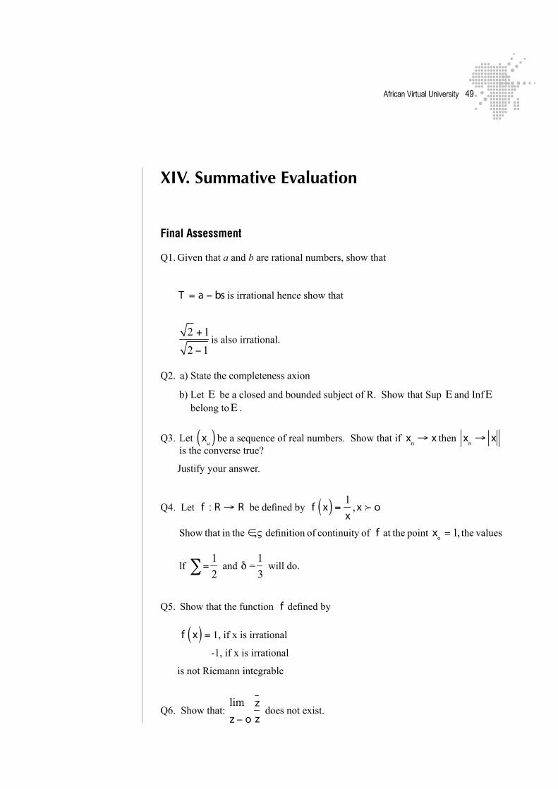
Q1. Given that a and b are rational numbers, show that

T = a − bs is irrational hence show that

2 +1

2 −1is also irrational.

Q2. a) State the completeness axion

b) Let Ε be a closed and bounded subject of R. Show that Sup Ε and InfΕ belong toΕ .

Q3. Let

xu( ) be a sequence of real numbers. Show that if xn → x then

x

n→ x

is the converse true?

Justify your answer.

Q4. Let f : R → R be defined by f x( ) = 1

x, x f o

Show that in the ∈,ς definition of continuity of f at the point xo= 1, the values

lf

=∑1

2 and δ =

1

3 will do.

Q5. Show that the function f defined by

f x( ) = 1, if x is irrational

-1, if x is irrational

is not Riemann integrable

Q6. Show that: limz − o

zz

does not exist.


Q7. Give the definition of an analytic function of a complex variable. Show that

f (2) = ez is not analytic anywhere.

Q8. By parameterising the complex number z evaluate: c12∫ dz where c is circle

within centre origin and radius R . Evaluate the same integral if C is any other circle which does not include the origin in its interior nor boundary. State any results you use.

Q9. Let r (t) be the position of a particle moving at constant speed.

(a) Show that the acceleration of the particle is orthogonal to the velocity of the object.

(b) For the vector valued function F (x, y, z) = x2i + ∂y2 j − zk find ∇F at the

point (2,−1,1)

Q10. It is known that a vector field F is called divergence free field if divF = 0

show that the vector field F (x, y, z) = x3 y2 zi + x2 z j + x2 yk is not divergence

free unless x = 0 or y = 0 or z = 0It is also known that a vector F is conservative if Curl F =0. Show that the sector field

F (x, y, z) = zxyi+(x2+z2) i+2zyk is conservative


Final assessment: Solutions

Q1. Assume t=a+bs is rational. Then we have that

bs = −(a − t)

s = −a − t( )

b=

t − ab

Since the set of rational numbers is closed under addition and multiplicationt − a

b.

But s is irrational. This is a contradiction. Hence it is irrational

Now 2 +12 −1

=2 +1( ) 2 +1( )2 −1( ) 2 +1( )

=2 + 2 + 2 +12 + 2 − 2 −1

= 3+ 2 2

1= 3+ 2 2

Since 3 and 2 are rational and 2 is irrational we have by the result that 3+ 2 2

is irrational. Hence 2 +12 −1

is irrational


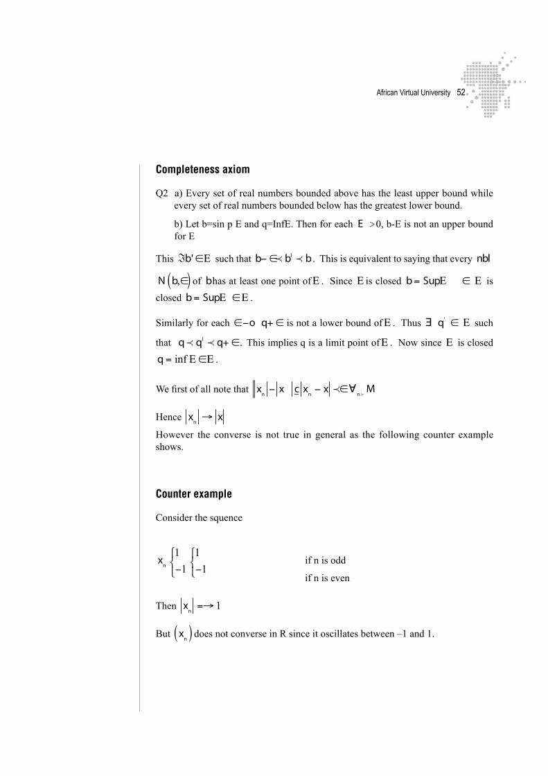
Completeness axiom

Q2 a) Every set of real numbers bounded above has the least upper bound while every set of real numbers bounded below has the greatest lower bound.

b) Let b=sin p E and q=InfE. Then for each E >0, b-E is not an upper bound for E

This ℑb' ∈Ε such that b− ∈p b1p b . This is equivalent to saying that every nbl

N b,∈( ) of bhas at least one point ofΕ . Since Ε is closed b= SupΕ ∈ Ε is

closed b= SupΕ ∈Ε .

Similarly for each ∈−o q+ ∈ is not a lower bound ofΕ . Thus ∃ q' ∈ Ε such

that q p q1

p q+ ∈. This implies q is a limit point ofΕ . Now since Ε is closed

q = inf Ε ∈Ε .

We first of all note that

xn− x c x

n− x p∈∀

nf

M

Hence x

n→ x

However the converse is not true in general as the following counter example shows.

Counter example

Consider the squence

xn

1

−1

⎧⎨⎩

1

−1

⎧⎨⎩

if n is odd

if n is even

Then x

n=→ 1

But

xn( ) does not converse in R since it oscillates between –1 and 1.


Q4. Given f x( ) = 1

x, x f o

we show that f is continuous at xo= 1.

Given in particular that ∈=

1

2 we have.

f x( ) − f 1( ) p∈⇒

1

x−1 p

1

2

⇒

1− xx

p

1

2

⇒

−1x −1( )1x1

p

1

2

⇒

x −1

1x1p

1

2

⇒ x −1 p

x

2

⇒ x −1 p

x2

for x f o

Now take S =

x2,

then

x −1 p δ ⇒

1

x−1 p

1

2

But since x is any positive number in particular let x =

2

3. Then we have

x −1 p δ =

1

3⇒1

1

x−1 p π

1

2


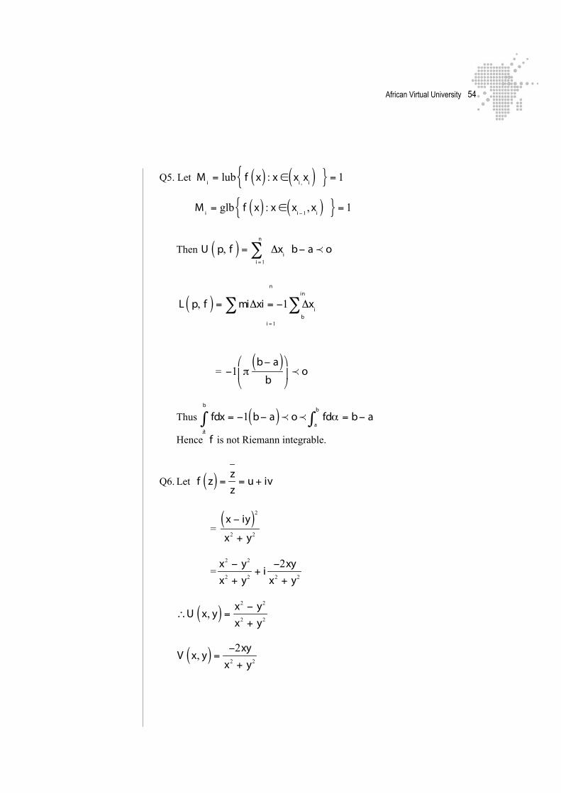
Q5. Let M

i= lub f x( ) : x ∈ x

i ,x

i( ) } = 1{

M

i= glb f x( ) : x ∈ x

i −1, x

i( ) } = 1{

Then U p, f( ) = ∑

i =1

n

Δxi b− a p o

L p, f( ) = miΔx∑ i = −1 Δxi∑

b

in

i =1

n

=

−1 πb− a( )

b

⎛

⎝⎜

⎞

⎠⎟ p o

Thus

fdx = −1 b− a( ) p o p fdα = b− a

a

b

∫a

b

∫ Hence f is not Riemann integrable.

Q6. Let f z( ) = z

z= u+ iv

=

x − iy( )2

x2 + y2

=

x2 − y2

x2 + y2+ i

−2xyx2 + y2

∴U x, y( ) = x2 − y2

x2 + y2

V x, y( ) = −2xy

x2 + y2


Now lim

U x,o( ) = limx2

x2= 1

x → o

limU o, y( ) = y2

y2= −1

y → o

Hence the limit doest not exist.

Q7. A function f z( ) of a complex variable is said to be analytic at Zo

if f z( ) is

differentiable at every Z in some nbl of Zo.

Given f Z( ) = ez

∴ f z( ) = ex − iy

= ex cos y − iSiny( )

Let U = ex cos y, V = −ex Siny

∂u∂x

= ex cos y

∂V∂x

= −ex Siny

∂u∂y

= −ex Siny

∂V2 y

= −ex cos y

∴

∂u∂y

≠∂v∂y

and

∂u∂y

≠∂v∂x


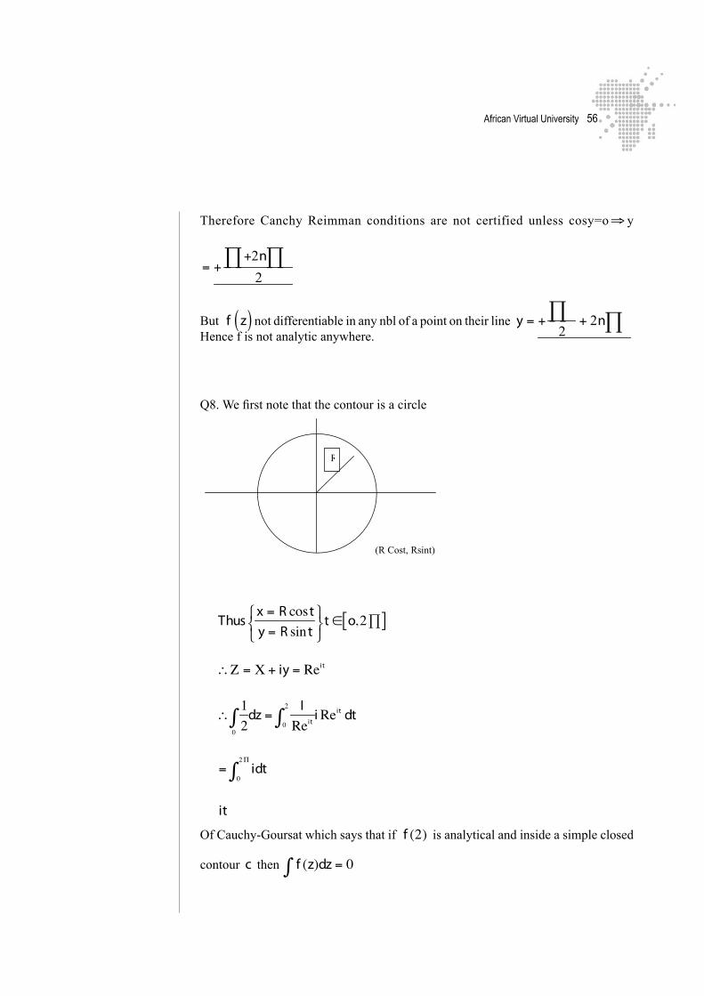
Therefore Canchy Reimman conditions are not certified unless cosy=o⇒ y

= +

+2n∏∏2

But f z( ) not differentiable in any nbl of a point on their line

y = +∏

2+ 2n∏

Hence f is not analytic anywhere.

Q8. We first note that the contour is a circle

R

(R Cost, Rsint)

Thusx = R costy = R sin t

⎧⎨⎩

⎫⎬⎭

t ∈ o,2∏[ ]

∴Ζ = Χ + iy = Reit

∴120∫ dz =

IReit0

2

∫ i Reit dt

= idt0

2Π

∫

it

Of Cauchy-Goursat which says that if f (2) is analytical and inside a simple closed

contour c then f (z)dz = 0∫


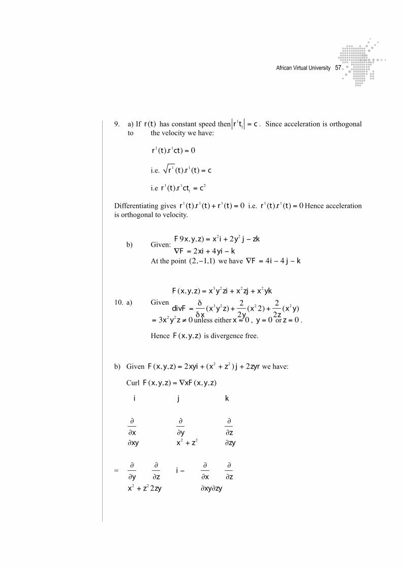
9. a) If r (t) has constant speed then r 1t1 = c . Since acceleration is orthogonal to the velocity we have:

r 1 (t).r 1ct) = 0

i.e. r 1 (t).r 1 (t) = c

i.e r 1 (t).r 1ct1 = c2

Differentiating gives r 1 (t).r 1 (t) + r 1 (t) = 0 i.e. r 1 (t).r 1 (t) = 0 Hence acceleration is orthogonal to velocity.

b) Given: F 9x, y, z) = x2i + 2y2 j − zk∇F = 2xi + 4yi − k

At the point (2,−1,1) we have ∇F = 4i − 4 j − k

10. a) Given

F (x, y, z) = x3 y2 zi + x2 zj + x2 yk

divF =δ

δx(x3 y2 z) + 2

2y(x2 2) + 2

2z(x2 y)

= 3x2 y2 z ≠ 0 unless either x = 0 , y = 0 or z = 0 .

Hence F (x, y, z) is divergence free.

b) Given F (x, y, z) = 2xyi + (x2 + z2 ) j + 2zyr we have:

Curl F (x, y, z) = ∇xF (x, y, z)

i j k

∂

∂x

∂

∂y

∂

∂z ∂xy x2 + z2 ∂zy

= ∂

∂y

∂

∂z i −

∂

∂x

∂

∂z

x2 + z2 2zy ∂xy∂zy


+ ∂

∂x

∂

∂x K

= 2xy x2 + z2

= (2z − 2z)i − (0 − 0) j + (2x + 2x)k= 0 − 0 + 0 = 0

Hence F (x, y, z) is conservative.


XV. ReferencesLarson Hostetler, Edwards, Calculus with analytic geometry, Houghton Mifflin Company New York 1988.

XVI. Main author of the ModuleThe author of this module on Basic Mathematics was born in 1953 and went through the full formal education in Kenya. In particular he went to University of Nairobi from 1974 where he obtained Bachelor of Science (B.Sc) degree in 1977. A Master of Science (M.Sc.) degree in Pure Mathematics in 1979 and a Doctor of Philosophy (P.HD) degree in 1983. He specialized in the branch of Analysis and has been tea-ching at the University of Nairobi since 1980 where he rose through the ranks up to an Associate Professor of Pure Mathematics.

He has over the years participated in workshop on development of study materials for Open and Distance learning program for both science and arts students in which he has written books on Real Analysis, Topology and Measure Theory.

Address

Prof. Jairus M. KhalagaiSchool of MathematicsUniversity of NairobiP. O. Box 30197 – 00100Nairobi – KENYAEmail: [email protected]

Analysis 1 Analysis 1 - · PDF fileAnalysis 1 Analysis 1. ... African Virtual University I....

Documents

Transcript of Analysis 1 Analysis 1 - · PDF fileAnalysis 1 Analysis 1. ... African Virtual University I....