Seminar series nr 137

Viktor Kalén

2007 Geobiosphere Science Centre Physical Geography and Ecosystems Analysis Lund University Sölvegatan 12 S-223 62 Lund Sweden

Analysing temporal and spatial variations in DOC concentrations in Scanian lakes and streams, using GIS and Remote Sensing

I

Viktor Kalén Degree thesis in Physical Geography and Ecosystem Analysis

Supervisor: Harry Lankreijer Department of Physical Geography and Ecosystem Analysis

Lunds University, 2007

Analysing temporal and spatial variations in

DOC concentrations in Scanian lakes and

streams, using GIS and Remote Sensing

II

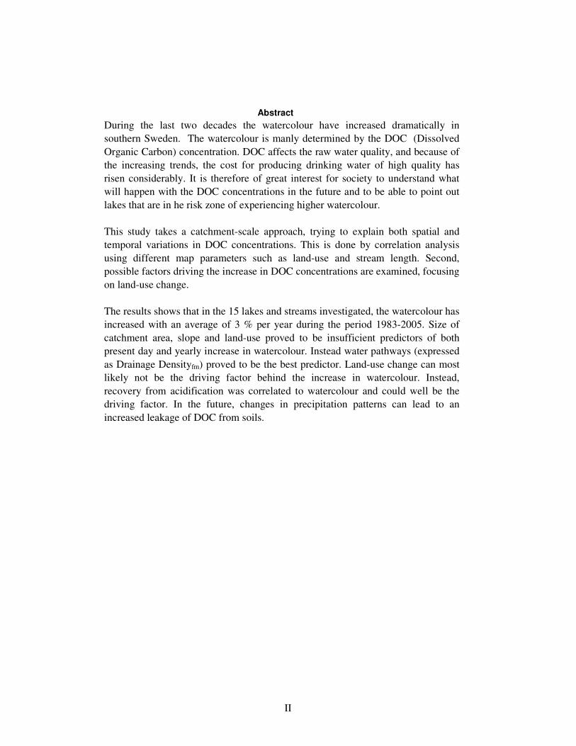
Abstract

During the last two decades the watercolour have increased dramatically in

southern Sweden. The watercolour is manly determined by the DOC (Dissolved

Organic Carbon) concentration. DOC affects the raw water quality, and because of

the increasing trends, the cost for producing drinking water of high quality has

risen considerably. It is therefore of great interest for society to understand what

will happen with the DOC concentrations in the future and to be able to point out

lakes that are in he risk zone of experiencing higher watercolour.

This study takes a catchment-scale approach, trying to explain both spatial and

temporal variations in DOC concentrations. This is done by correlation analysis

using different map parameters such as land-use and stream length. Second,

possible factors driving the increase in DOC concentrations are examined, focusing

on land-use change.

The results shows that in the 15 lakes and streams investigated, the watercolour has

increased with an average of 3 % per year during the period 1983-2005. Size of

catchment area, slope and land-use proved to be insufficient predictors of both

present day and yearly increase in watercolour. Instead water pathways (expressed

as Drainage Densityfm) proved to be the best predictor. Land-use change can most

likely not be the driving factor behind the increase in watercolour. Instead,

recovery from acidification was correlated to watercolour and could well be the

driving factor. In the future, changes in precipitation patterns can lead to an

increased leakage of DOC from soils.

III

Sammanfattning

Under de två senaste decennierna har vattenfärgen ökat dramatiskt i södra Sverige.

Vattenfärgen bestäms främst av koncentrationen av humuspartiklar. Humus

påverkar råvattenkvalitén och kostnaden för att producera dricksvatten har ökat

markant p.g.a. de ökande humushalterna. Det är därför av stort intresse för

samhället att kartlägga vad som kommer hända med DOC koncentrationerna i

framtiden och peka ut sjöar som är i riskzonen för ökande vattenfärg.

I den här studien analyseras både spatiala och temporal variationer i DOC

koncentrationer. Detta görs genom korrelationsanalyser mellan olika

kartparametrar och vattenfärgsvärden. Möjliga förklaringar till vad som kan vara

den drivande faktorn bakom vattenfärgsökningen undersöks, med fokus på

förändrad markanvändning.

Resultaten visar på att i de 15 sjöar och vattendrag som undersökts har

vattenfärgen ökat med i genomsnitt 3 % per år under perioden 1983-2005. Storlek

på avrinningsområdet, lutning samt markanvändning visade sig ha låg

förklaringsgrad, både vad gäller årlig ökning i vattenfärg samt aktuell vattenfärg.

Istället visade sig vattnets flödesvägar i avrinningsområdet (utryckt som Drainage

Densityfm) ha den bästa förklaringsfaktorn. Detta resultat visar på att dikning av

skog- och myrmark starkt påverkar vattenkvaliteten, vilket är vikigt att ta hänsyn

till vid framtida rensningar och dikningar

Förändrad markanvändning, från öppen mark till skogsmark, kan med störst

sannolikhet inte vara den drivande faktorn bakom vattenfärgsökningen. Dock har

andelen skogsmark ökat och kan väl ha bidragit till en del av ökningen i vattenfärg.

Istället verkar minskat svavelnedfall vara den faktor som driver förändringen, detta

genom att göra DOC - partiklarna mer lättrörliga och på så sätt öka läckaget. Den

stora ökning i vattenfärg som observerats kanske är en ”ursköljningsprocess” av

kol som varit starkare bundet när svavelnedfallet var högre. Resultaten visar också

på förändringar i vattnets ursprung mellan 1980- och 2000 talet, med ett större

inslag av regnvatten. Orsaken till detta skulle kunna vara ökad nederbörd eller

förändrade nederbördsmönster, men också djupare och/eller fler dikningar i skog

och myrmark. Framtida klimatförändringar spår både ökade nederbördsmängder

och förändringar i nederbördsmönster, något som kan leda till ökat läckage av

DOC till sjöar och vattendrag.

1. Introduction ______________________________________________________ 3

1.1 Aim__________________________________________________________ 4

2. Theoretical background ___________________________________________ 5

2.1 What is watercolour? _________________________________________ 5

2.2 How is watercolour measured? ________________________________ 5

2.3 Where does DOC come from? _________________________________ 5

2.4 The magnitude of carbon exported from catchments ____________ 7

2.5 Parameters effecting watercolour ______________________________ 7

2.6 Possible factors driving the increase___________________________ 8

3. Method __________________________________________________________ 9

3.1 Absorbance and water chemistry data ________________________ 10 3.1.1 Selection of lakes and streams ________________________________ 10 3.1.2 Compilation and statistics for absorbance values __________________ 11 3.1.2 Compilation and statistics for absorbance values __________________ 12

3.2 Generating the catchment areas ______________________________ 12 3.2.1 Modelling the catchment areas ________________________________ 12 3.2.2 Evaluation and updating of the catchment areas___________________ 13

3.3 Map parameters in the catchment areas _______________________ 13 3.3.1 Description of land-use data (SMD-data)________________________ 13 3.3.2 Land use in all 15 catchment areas _____________________________ 14 3.2.3 Land use in the near- and surrounding of streams and watercourses ___ 14 3.2.4 Drainage density ___________________________________________ 15 3.2.6 Statistical analysis – map parameters ___________________________ 15

3.3 Quantifying land-use change by aerial interpretation ___________ 16 3.3.1 Selecting catchment areas for interpretation______________________ 16 3.3.2 Aerial photographs _________________________________________ 16 3.3.3 Georeferencing the 1980-pictures______________________________ 17 3.3.4 Interpretation of the aerial photographs _________________________ 18 3.3.5 Field control and thematic accuracy ____________________________ 18

3.4 Precipitation and sulphur deposition__________________________ 19

4. Results _________________________________________________________ 21

4.1 Comparison between initial and present day values ____________ 21

4.3 Correlations between map parameters and absorbance ________ 23 4.3.1 Present day absorbance______________________________________ 23 4.3.2 Yearly increase in absorbance ________________________________ 25

4.4 Land use change ____________________________________________ 27 4.4.1 Cross-table evaluation points _________________________________ 27 4.4.2 Thematic accuracy _________________________________________ 28

2

4.4.3 Land use change – interpretation of aerial photographs _____________ 28

4.5 Other possible explanations driving the increase in absorbance 30 4.5.1 Precipitation and sulphur-deposition ___________________________ 31 4.5.2 E.C.-I.R. Diagram __________________________________________ 33

5. Discussion ______________________________________________________ 35

5.1 Absorbance values __________________________________________ 35

5.2 Map parameters _____________________________________________ 35

5.3 Land-use change ____________________________________________ 36

5.4 Other explanations driving the increase _______________________ 37

5.5 Lake Liasjön and drainage of forested areas___________________ 38

6. Conclusions_____________________________________________________ 40

7. References______________________________________________________ 41

3

1. Introduction

There is overwhelming evidence that the watercolour has increased during the last two

decades across Europe and North America (Evans 2004). The same trend is observed in

southern Sweden (Lövgren 2003). The average watercolour in Sweden has increased

with ~3% each year during the two last decades (SLU). The watercolour is mainly

determined by the content of humic substances (the Swedish Environmental Protection

Agency 1999), which originate mainly from decomposition of organisms, mostly

decaying plants. Humic substances absorb light, giving water rich in humus a high

watercolour (Evans 2004).

In Sweden approximately 25% of the people receive their drinking water from

groundwater, 25 % from artificial filtration of surface water, and 50 % gets their water

from lakes and streams (Lövgren 2003). The main difference between groundwater and

surface water is their variation in humic substances. Groundwater contains very low

values while surface water exhibits large variations both in time and space (Thurman

1985). Humic substances create huge problems for water treatment plants trying to

produce drinking water of high quality. Since humic substances is a source of energy

for micro organisms it can contribute to bacterial growth in the water distribution

systems, causing diseases and giving the water bad taste and odour (Lövgren 2003).

Humus and added chlorine can form chlor-organic compounds that are very

carcinogenic (Sibelle 1988). The increase in watercolour means that the cost for

producing drinking water of a high quality has risen dramatically. Some municipalities

even evaluate the possibility of switching to other water supplies with better quality,

e.g. ground water supplies or other surface water supplies with lower humic content.

Because of this it is of great interest for society to understand weather the humus

concentrations will continue to raise, level out or return to more acceptable values

(Lövgren 2003). It is also interesting to identify lakes that can be experiencing

increasing humic content in the future (SLU a)

According to the EUs water framework directive (established in 2000) all surface

waters shall have a “good ecological status” in the year of 2015. Organic matter

influences almost every process in the aquatic environment (Thurman 1985). Since it

plays a significant role in aquatic food webs, transports of nutrients and metals, and

modifies the optical properties of water bodies (Findlay and Sinsabaugh 2003) it is of

great interest to understand why the watercolour increases. There are many theoretical

hypotheses on these trends. The three hypotheses examined in this work can be summed

to three major areas; a) changes in land-use (LUSTRA 2002), b) climate related changes

such as precipitation and temperature (Neal et al., 2005) and c) recovery from

acidification (Evans et al. 2006).

4

1.1 Aim

Inland water functioning is tightly linked to the characteristics of their catchment areas

(Kalff 2002). This study will take a catchment scale approach; first trying to explain

spatial variations, and second temporal variations in watercolour.

This thesis aims to give the answer to the following questions:

1. Is the increase in watercolour for the data used in this work of the same magnitude

as reported in literature?

2. How accurate is a catchment area modelled using a DEM (Digital Elevation Model)

compared to drawing it using the topographic map?

3. Which map parameter can best explain the spatial and temporal variation in

watercolour?

4. Can land-use change be the driving factor behind the increased watercolour?

5. Can changes in precipitation, sulphur deposition or changes in water origin explain

the increased watercolour?

5

2. Theoretical background

2.1 What is watercolour?

Total Organic Carbon (TOC) is the sum of all organic carbon species found in water,

from methane to larger and more complex humic substances. TOC can be divided into

Particulate (POC) and Dissolved Organic Carbon (DOC) by filtration through a 0.45

µm net. The majority of the DOC are polymeric organic acids, also called humic

substances (Thurman 1985). Humic substances absorb visible light, most strongly at the

blue end of the spectrum, thus giving waters rich in DOC a characteristic brown colour

(Evans 2004).

2.2 How is watercolour measured?

The most common method to measure watercolour is based on a visual comparison

between the water sample and a solution containing Potassium Hexachloroplatinate

(K2PtCl2 unit mg Pt L-1) (Brönmark and Hansson, 2005). The method used for the data

in this work is based on absorbance measurements. The measurements are made at the

wavelength 420 nm in a 5 cm cuvette on filtrated water (0.45 µm) (SLU b). This

method is supposed to be a measure of humic substances, but the absorbance

measurements can be influenced by several other factors, such as; ionic strength, pH,

light scattering and the presence of other light absorbing substances, mainly iron/

manganese-oxides and nitrate (Temnerud 2005). Since iron (and most other metals)

bond with dissolved organic molecules (Kalff 2002) an increase in DOC content will

lead to an increase in iron (and other metals). How much these other factors influence

the absorbance values is not well known and it falls outside the aim of this work.

However, according to the Swedish Environmental Protection Agency (report 4913,

1999) a high humic content gives higher absorbance. In the report they also conclude

that absorbance measurements are an objective and more accurate method than the one

based on visual comparison. Throughout this work it is supposed that a higher

DOC/humic- content gives a higher absorbance and thereby higher water colour.

2.3 Where does DOC come from?

DOC is generated by the partial decomposition of, or exudation from, organisms (Evans

et al 2004). The DOC produced in the lake or stream is referred to as autochthonous

sources, and DOC produced outside the lake or stream is referred to as allochthonous

sources. The major of the DOC in streams and small to moderate-size rivers comes

from allochthonous sources (Thurman 1985).

The allochthonous sources can mainly be divided into two categories, organic matter

from soils and organic matter from plants. The organic matter from soil has

decomposed for a longer time and is of older age than the organic matter from plants

6

(Thurman 1985). Radiocarbon studies have shown that most of the DOC in streams and

lakes is derived from material of much younger age than the organic soil material. This

means that most of the DOC in lakes and streams is derived from resent terrestrial

primary production. Leaching from fresh deciduous litter may explain the seasonality in

the concentration of DOC in discharge from forested catchments. This because

deciduous leaf litter imparts high DOC concentrations in the autumn, while coniferous

litter and organic soils release DOC more evenly. (Hongve 1999).

The organic carbon content is highest in the upper soil layers and decreases with depth.

The O-horizon consists of ~ 20 % organic carbon and the C-horizon less than 2 %.

Interstitial water (water between pores) easily solubilize organic matter from the litter

layer (O-horizon). The organic matter dissolved is mostly DOC originating from

decaying processes of plants and soil. The interstitial water carries the DOC into the A

and B-horizons. Because of adsorption and decaying processes in soil, the content of

DOC in interstitial water decreases with depth (Figure 1) (Thurman 1985). This gives a

sharp attenuation of DOC as water moves from upper soil horizons to lower soil

horizons and in to the saturated zone (Cronan and Aiken 1984). This means that water

transported only through the upper soil layers have a higher concentration of DOC,

compared to water transported further down in soil.

Figure 1. The DOC content of interstitial water decreases rapidly with depth. This is due to low decreasing carbon content as well as adsorption and degradation process in soil (From Thurman 1985).

7

2.4 The magnitude of carbon exported from catchments

On a global scale, one percent of terrestrial NEP (Net Ecosystem Production) is

exported to rivers and lakes (Kalff 2002). According to Worral et al. (2006) the leakage

from a catchment area mostly covered by peat can range between 4.0 to 7.0 g C m-2 yr-1.

Lövgren (2003) reported values between 1 to 20 g C m-2 yr-1 for alpine and boreal

catchments in the Nordic region.

It is mostly the concentration of humic substances that relegate the emission of CO2

from lakes (Vetenskapsrådet), thereby would an increase in DOC concentrations give an

increase in the amount of CO2 evaded from lakes and streams. Dillon and Mollot (1997)

compared their catchment export rates with NEP for American forests (data from

Edwards et al.1981; Whittaker et al. 1979). By doing this they estimated that up to 5 %

of NEP from a forest can be returned to the atmosphere as CO2 through lake evasion.

Jonsson et al. (2006) investigated the export of terrestrially fixed carbon to aquatic

systems in a boreal catchment in northern Sweden. They concluded that approximately

3 % of the terrestrial NEE (Net Ecosystem Exchange) is evaded as CO2 in lakes and

streams.

2.5 Parameters effecting watercolour

Several possible explanations on factors in a catchment area that cause high water

colour have been discussed. Among these, the following factors have been investigated

in this work:

Land-use: The Land-use in the catchment area is often used to explain DOC

concentrations in lakes and streams. According to Lövgren et al. (2003) high humus

concentrations is found in catchments with large soil pools of carbon, such as peat and

frosted areas, and short water retention times. According to Dillon and Mollot (1997),

the percentage of peat coverage in a catchment area is positively correlated to the DOC

concentrations. This is because DOC is probably readily leached from peat lands

because of the persistent moisture saturation, and the high carbon content (Kalff 2003).

Drainage Density: By summarizing the total length of streams in a catchment area and

dividing it by the size of catchment area, the drainage density is calculated. A low

drainage density means that a particle has to travel further to reach a stream before it

can be exported (Kalff 2003). Or expressed in another way, drainage density gives a

measure of the average lateral flow path length through soil to the stream network

(Dahlström 2005). A long flow path would mean that the water floats at lower depths in

soil, and DOC will then be adsorbed and the concentration of DOC in water will

decrease (according to the theory discussed in section 2.3). This argument is in line with

the work of Hope et al. (1994) where they suggest that concentrations of DOC in stream

water are usually strongly linked to catchment hydrological pathways. Hongve (1999)

8

argues that the water pathways through the soil probably are the most important factor

determining the DOC concentrations in lakes and streams.

Slope and size of catchment area: The slope of the catchment area is usually

correlated to the amount particles exported. If a catchment area has a high average

slope, particles (in this case DOC) leave land at higher rate per unit area. A small

catchment area usually has a higher average slope (Kalff 2001).

2.6 Possible factors driving the increase

The cause of the increase in watercolour has been discussed widely in the literature.

Roulet and Moore (2006) concludes that the increasing trends in DOC concentrations

has to do with either an increase in net DOC production in terrestrial ecosystems, or

increases in leaching of DOC. This study focuses on three explanations on why the

watercolour increases:

Land- use change: Planting forest on agricultural land increases the humic content in

the upper part of the soil (LUSTRA 2002); this would lead to an increase in DOC

exported to lakes and streams. During the last decades there has been an observed

increase of carbon content in the upper soil parts (Vetenskapsrådet), this raises the

question whether the increased forest production can be coupled to the increasing

absorbance values.

Precipitation: Long-term increases in precipitation will raise the groundwater level so

it comes in contact with the organic soils and transports DOC to lakes and streams.

(Lövgren et al. 2003). An increase in stream discharge gives an increase in DOC

concentrations, due to a “flushing effect” in the upper soil layers (Hope et al. 1994).

Recovery from acidification: Today, the average sulphur deposition in Sweden has

decreased to approximately one third of the levels in 1988 (SLU 2007). DOC solubility

is suppressed by high soil water acidity and ionic strength. Thereby would a decline in

sulphur deposition lead to increased release of DOC from soils (Evans et al. 2006).

9

3. Method

The method can be divided into five main steps. 1) Compilation of absorbance data for

15 different test points, 2) generating of catchment areas for the fifteen test points, 3)

quantification of land-use and other map parameters in the catchment areas, 4)

interpretation of aerial photographs to test if land-use change can be the driving factor

behind the increased watercolour and 5) test other possible explanations of what can be

the driving factor behind the increased watercolour (Figure 2).

Figure 2. Conceptual model of the general steps used in the method.

3. Land-use and other map parameters in all catchment areas

• Land use in whole catchment area

• Land use close to watercourses

• Drainage density

• Slope

5. Other possible explanations driving the increase in watercolour

• Decreased sulphur deposition

• Changes in precipitation

• Changes in water origin (groundwater to surface water)

1. Absorbance data

• Selection

• Compilation

• Statistics

2. Generating catchment areas

• Modeling (using a DEM)

• Evaluation

• Updating

4. Land-use change by interpretation of aerial photographs

• Land-use from three different

time spans: 1940, 1980 and

2000

Witch map parameter is the best predictor of observed and increased absorbance?

Possible explanations to the driving factor behind the increase in absorbance

10

3.1 Absorbance and water chemistry data

SLU (Sveriges lantbruksuniversitet) has a commission from the Swedish government to

run continuous environmental analysis, as a part of the National and Regional

environmental surveillance. The commission is divided into ten different areas; of witch

lakes and streams is one. This part of the program aims to follow variations between

years and changes over time. The test points selected for the program are a

representative (for Sweden) selection of lakes and streams that are not directly affected

by emissions or intensive land-use. The result is to be used as a reference in comparison

with more affected lakes and streams. All water chemical data used in this work

(absorbance, chlorine (Cl-), calcium (Ca2+) and conductivity) is downloaded from the

SLU website (http://www.ma.slu.se/).

3.1.1 Selection of lakes and streams

In Scania there are over 100 test points included in the environmental analyses. Not all

of these were examined in this work. To be used in this work the test points had to fulfil

the following criteria’s.

• Since the main objective of the work is focusing of explaining temporal change

based on spatial parameters the test points had to have time series longer than

15 years.

• Since this work is done in cooperating with the County Administrative board of

Scania, and since the data used for land-use and map parameters only covers

Scania the catchment area for the lake/stream had to be inside (or close to) the

Scanian borders.

These criteria’s gave a total of 15 test points, 8 lakes and 7 streams. (Figure 3)

11

R å å nR å å n

B ä e nB ä e n

R ö n n e å nR ö n n e å n

To s t a r pTo s t a r p

S t e n s å nS t e n s å n L i a s j ö nL i a s j ö n

L i l l e s j öL i l l e s j ö

To l å n g a å nTo l å n g a å n

F å g l a s j ö nF å g l a s j ö n

S k i v a r p s å nS k i v a r p s å n

K l i n g a v ä l s å nK l i n g a v ä l s å n

T r o l l e b ä c k e nT r o l l e b ä c k e nS k ä r a v a t t n e tS k ä r a v a t t n e t

S v a n s h a l s s j ö nS v a n s h a l s s j ö n

L ä r k e s h o l m s s j ö nL ä r k e s h o l m s s j ö n

0 20 4010Kilometers �Viktor Kalén (2007). Bakgrundskartor Lantmäteriet dnr 106-2004/188

1:1 000 000

Figure 3. The 15 test points and their catchment areas (for method

generating catchment areas, see section 3.2).

12

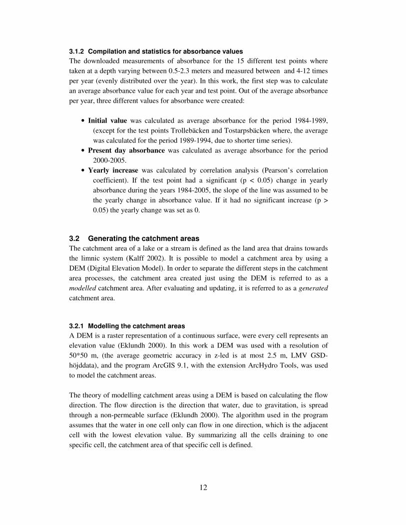
3.1.2 Compilation and statistics for absorbance values

The downloaded measurements of absorbance for the 15 different test points where

taken at a depth varying between 0.5-2.3 meters and measured between and 4-12 times

per year (evenly distributed over the year). In this work, the first step was to calculate

an average absorbance value for each year and test point. Out of the average absorbance

per year, three different values for absorbance were created:

• Initial value was calculated as average absorbance for the period 1984-1989,

(except for the test points Trollebäcken and Tostarpsbäcken where, the average

was calculated for the period 1989-1994, due to shorter time series).

• Present day absorbance was calculated as average absorbance for the period

2000-2005.

• Yearly increase was calculated by correlation analysis (Pearson’s correlation

coefficient). If the test point had a significant (p < 0.05) change in yearly

absorbance during the years 1984-2005, the slope of the line was assumed to be

the yearly change in absorbance value. If it had no significant increase (p >

0.05) the yearly change was set as 0.

3.2 Generating the catchment areas

The catchment area of a lake or a stream is defined as the land area that drains towards

the limnic system (Kalff 2002). It is possible to model a catchment area by using a

DEM (Digital Elevation Model). In order to separate the different steps in the catchment

area processes, the catchment area created just using the DEM is referred to as a

modelled catchment area. After evaluating and updating, it is referred to as a generated

catchment area.

3.2.1 Modelling the catchment areas

A DEM is a raster representation of a continuous surface, were every cell represents an

elevation value (Eklundh 2000). In this work a DEM was used with a resolution of

50*50 m, (the average geometric accuracy in z-led is at most 2.5 m, LMV GSD-

höjddata), and the program ArcGIS 9.1, with the extension ArcHydro Tools, was used

to model the catchment areas.

The theory of modelling catchment areas using a DEM is based on calculating the flow

direction. The flow direction is the direction that water, due to gravitation, is spread

through a non-permeable surface (Eklundh 2000). The algorithm used in the program

assumes that the water in one cell only can flow in one direction, which is the adjacent

cell with the lowest elevation value. By summarizing all the cells draining to one

specific cell, the catchment area of that specific cell is defined.

13

3.2.2 Evaluation and updating of the catchment areas

To evaluate how accurate the modelled catchment areas where, the modelled result from

the test point Lake Liasjön was compared to the same catchment area drawn from the

topographic map (scale 1:50 000). The drawing was made by Anna Hagerberg at the

County Administrative Board of Scania, and the result was seen as the “true” catchment

area of Lake Liasjön. The information used from the topographic map was primarily the

height from contour lines, but also the location and drainage direction of wetlands,

small waters and streams.

The information of drainage direction of wetlands and flow directions of streams gave

additional information that could not be modelled only using the DEM as input (see

results, section 4.2). To get the catchment areas as correct as possible these parameters

had to be taken into account. Thereby, the modelled catchment areas had to be

controlled and sometimes adjusted. As a help with controlling and updating the

catchment areas, borders from SMHIs sub catchments were used. The modelled areas

where controlled and adjusted by controlling each line segment by the following

process:

• If the line segments of the modelled result agreed with SMHIs boundaries, and

if there were no obvious errors (e.g. streams running across the border of the

catchment area), the line segments were accepted as correct modelled.

• If the line segments of the modelled result where close to SMHIs borders, a

comparison was made with the topographic map, to see if the modelled result or

SMHI had the best fit.

• Most of the time the line segment were far away from the SMHI boarders. In

these cases the catchment areas were compared to the topographic map. If there

where no obvious errors, the line segments were classed as correct modelled.

3.3 Map parameters in the catchment areas

Three different main groups of map parameters were created for correlation analysis

with absorbance values; these where Land-Use, Drainage Density and Size/Slope.

3.3.1 Description of land-use data (SMD-data)

To quantify the land-use in all the 15 catchment areas, SMD-data (Svensk Marktäckedata) was

used. This is a database containing national land cover and land use data that is based on EUs

classification system for CORINE Land Cover. The difference between CORINE-data and

SMD-data is that the SMD database is suited for Swedish conditions and land cover (total 57

classes). The main data source for the database is multispectral satellite images (Landsat TM)

and therefore the geometric resolution of the database is 25*25 m. The thematic accuracy for

the SMD-data is 75 % and the geometric accuracy is 25 m (one pixel). The database is

14

produced in the reference system RT90, and produced raster data and then converted to vector

data, which is used in this project (LMV-produktspecifikation).

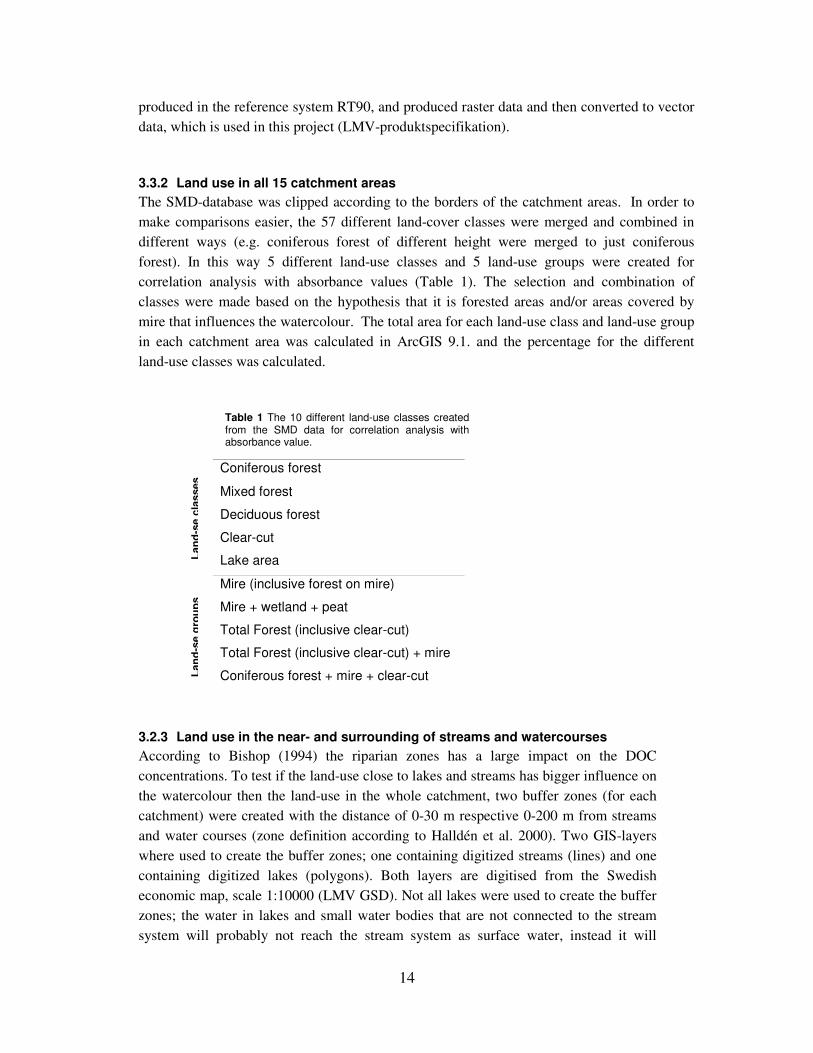
3.3.2 Land use in all 15 catchment areas

The SMD-database was clipped according to the borders of the catchment areas. In order to

make comparisons easier, the 57 different land-cover classes were merged and combined in

different ways (e.g. coniferous forest of different height were merged to just coniferous

forest). In this way 5 different land-use classes and 5 land-use groups were created for

correlation analysis with absorbance values (Table 1). The selection and combination of

classes were made based on the hypothesis that it is forested areas and/or areas covered by

mire that influences the watercolour. The total area for each land-use class and land-use group

in each catchment area was calculated in ArcGIS 9.1. and the percentage for the different

land-use classes was calculated.

3.2.3 Land use in the near- and surrounding of streams and watercourses

According to Bishop (1994) the riparian zones has a large impact on the DOC

concentrations. To test if the land-use close to lakes and streams has bigger influence on

the watercolour then the land-use in the whole catchment, two buffer zones (for each

catchment) were created with the distance of 0-30 m respective 0-200 m from streams

and water courses (zone definition according to Halldén et al. 2000). Two GIS-layers

where used to create the buffer zones; one containing digitized streams (lines) and one

containing digitized lakes (polygons). Both layers are digitised from the Swedish

economic map, scale 1:10000 (LMV GSD). Not all lakes were used to create the buffer

zones; the water in lakes and small water bodies that are not connected to the stream

system will probably not reach the stream system as surface water, instead it will

Table 1 The 10 different land-use classes created from the SMD data for correlation analysis with absorbance value.

Lan

d-s

e g

rou

ps

Lan

d-s

e c

lasses

Coniferous forest

Mixed forest

Deciduous forest

Clear-cut

Lake area

Mire (inclusive forest on mire)

Mire + wetland + peat

Total Forest (inclusive clear-cut)

Total Forest (inclusive clear-cut) + mire

Coniferous forest + mire + clear-cut

15

percolate down to the groundwater which means that DOC will be absorbed before

reaching the stream network (see section 2.3). Because of this, lakes without a line

segment within 30 m from the stream network were excluded before creating the buffer

zone.

The SMD-data was clipped according to the buffer-zones. The total area for each land-

use class in the buffer-zones and catchment area was calculated in ArcGIS 9.1 and the

percentage for the different land-use classes was calculated.

3.2.4 Drainage density

Drainage density is the total length of streams divided by size of catchment area (unit

m/km2). Drainage Density was calculated by using a database containing all streams in

Scania (LMV GSD). This database only included streams with a width < 6 meters.

Because of this, streams wider than 6 meters had to be digitised from the economic

map. Two different measures of drainage density where calculated; Total Drainage

Density and Drainage Densityfm, which is drainage density for streams running through

forest and mire. A catchment area with a high percentage forest and mires will, in most

cases, get a higher Drainage Density fm and this value can be considered as a

combination of Drainage Density and land-use.

3.2.5 Slope

The slope was calculated in ArcGIS 9.1 using a DEM (described in section 3.2.1). The

slope is defined as the maximum change between each cell and its neighbours. This

gives each cell a slope value; a cell with a low slope value has a flat terrain. Two

different measurements of slope were created; 1) average slope calculated for all cells in

each of the 15 catchment areas, and 2) average slope for all cells covered by forest in

each of the 15 catchment areas.

3.2.6 Statistical analysis – map parameters

The land-use classes generated from the SMD-data were tested for correlations with

absorbance value. Both yearly increase in absorbance and present day absorbance value

were tested. The same was done for the other map parameters; Size of catchment area,

average Slope in catchment area, average Slope in forested areas, Drainage Density and

Drainage Densityfm. This gives that a total of 34 map parameters were tested for

correlations with absorbance values. The statistical method used was Pearson’s

Correlation Coefficient.

16

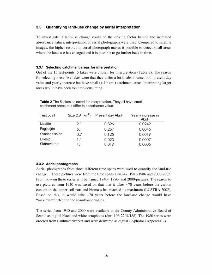
3.3 Quantifying land-use change by aerial interpretation

To investigate if land-use change could be the driving factor behind the increased

absorbance values, interpretation of aerial photographs were used. Compared to satellite

images, the higher resolution aerial photograph makes it possible to detect small areas

where the land-use has changed and it is possible to go further back in time.

3.3.1 Selecting catchment areas for interpretation

Out of the 15 test-points, 5 lakes were chosen for interpretation (Table 2). The reason

for selecting these five lakes were that they differ a lot in absorbance, both present day

value and yearly increase but have small (< 10 km2) catchment areas. Interpreting larger

areas would have been too time-consuming.

3.3.2 Aerial photographs

Aerial photographs from three different time spans were used to quantify the land-use

change. These pictures were from the time spans 1940-47, 1981-1986 and 2000-2005.

From now on these series will be named 1940-, 1980- and 2000-pictures. The reason to

use pictures from 1940 was based on that that it takes ~70 years before the carbon

content in the upper soil part and biomass has reached its maximum (LUSTRA 2002).

Based on this, it would take ~70 years before the land-use change would have

“maximum” effect on the absorbance values.

The series from 1940 and 2000 were available at the County Administrative Board of

Scania as digital black and white ortophotos (dnr- 106-2204/188). The 1980 series were

ordered from Lantmäteriverket and were delivered as digital IR-photos (Appendix 2).

Test point Size C.A (km

2) Present day AbsF Yearly increase in

AbsF

Liasjön 2.1 0.826 0.0242 Fåglasjön 6.1 0.267 0.0045 Svanshalssjön 0.7 0.125 0.0019 Lillesjö 1.1 0.023 0.0007 Skäravattnet 1.1 0.019 0.0005

Table 2 The 5 lakes selected for interpretation. They all have small catchment areas, but differ in absorbance value.

17

3.3.3 Georeferencing the 1980-pictures

The digital IR-pictures were only central projected, which means that the surface is

projected as a photography through a convex lens. The IR-pictures therefore had to be

linked to the same map projections as the two other orthophotos. This can be done in

two ways. The best result is achieved by a 3-dimensional correction with an adjustment

to a Digital Elevation Model (ortophoto production). This is a very expensive method

and was therefore not used in this work. Instead, a 2-dimensional adjustment was

chosen. This was done by determining transformation parameters by locating so called

Ground Control Points (GCPs). GCPs are points that can be clearly identified in the

image and in a source; which is in the required map projection system (in this case the

black and white orthophoto from 2000 in RT 90). Examples of GCPs can be road

intersection and house corners (Janssen and Hurnemann 2001).

Based on the set of GCPs, the pictures were transformed using a best fit procedure

(Janssen and Hurnemann 2001). The errors that remain after the transformation are

called residual errors. By summarizing these errors an RMS (Root Mean Square error)

value is calculated. This is an indicator of the quality of the transformation. The RMS

error is only valid for the area bounded by the GCPs, and therefore it is important to

select points close to the edge of the image (Janssen and Hurnemann 2001). After the

transformation, the pictures were geocoded by resampling the pictures. The

interpolation method used was nearest neighbour.

One picture (covering lake Liasjön) was already rectified in another project (Andersson,

thesis nr 110). For 3 of the 4 pictures rectified in this work, a 2nd order polynomial

transformation was used and the number of GCPs varied between 40-60. The exception

was the picture covering Lake Lillesjö. The lake (and it’s catchment area) is situated on

a height, which gives distortions in the geometric relationship caused by terrain

differences, so-called relief displacement (Janssen and Hurnemann 2001). Another

factor causing problems was the non even distribution of possible GCPs. Because of

this few (24) GCPs and a 3rd order polynomial was used (Appendix 2). This gave a

very bad fit in the outer parts of the picture, so-called Runges phenomena (Eklundh

2001) but it gave the best possible fit for the area of interest.

18

3.3.4 Interpretation of the aerial photographs

The interpretation was made by identifying and digitising homogenous objects (e.g.

areas with coniferous forest), in ArcGIS 9.1. As a help during the interpretation the

SMD-data as well as the other two aerial photos from the different time spans were

used. The land-use classes interpreted are shown in Table 3

In this way three different databases, one for each time span, were created for each

catchment area. The total area for each land-use class and time span was calculated in

ArcGIS 9.1. and the percentage for the different land-use classes was calculated.

3.3.5 Field control and thematic accuracy

Two field controls where made (13 and 24 of April 2007). The first time, areas where

the interpretation was uncertain were visited (training areas). The second time,

evaluation points where collected. The evaluation points where used to calculate the

thematic accuracy of the interpreted map. A stratified sample method was used where it

was made sure that all classes had evaluation points. Two kinds of selections were made

on the points; first, they had to be close to roads (<100 m) in order to get as many points

as possible and second, classes that were estimated as easy to interpret (e.g. water) got

fewer point. The evaluation values were calculated in three different ways, according to

Eklundh (2000):

• User Accuracy (Ai) is the probability that a random point on the map is correct

classified.

• Producer accuracy (Bi) is the probability that a random point in the reality is

correct classified.

• Kappa value (Kappa) gives a number between –1 to 1 and expresses to what

extent the points in the evaluated map differ from a random class. For example a

Kappa value of e.g. 0.5 means that the interpretation is 50 % better than chance.

Table 3 The land-use classes used in the aerial interpretation.

Artificial ground

Coniferous Forest

Mixed Forest

Clear cut/Young forest

Deciduous Forest

Mire

Water

Field/Open land

19

3.4 Precipitation and sulphur deposition

The data for precipitation and sulphur deposition was downloaded from the IVL,

Svenska Miljöinstitutet, website. The data is included in the same National environment

surveillance as the absorbance and water chemistry data. The data is delivered as

average per hydrologic year (the hydrologic year starts in October and ends in

September). Because of this the absorbance values for Lake Bäen were recalculated to

average absorbance for each hydrologic year (although, in the results the hydrologic

year is presented as one year value, e.g. 1988/1989 is presented as 1988). The sulphur

deposition measurements were made as both wet and dry deposition (IVL).

The station Arkelstorp (RN 1382500: 6212500) had the longest time series of sulphur

measurements (1989-2005) and was selected for correlations with absorbance values.

The catchment area closest to this station is the one for Lake Bäen (distance 11 km2)

and it was chosen for comparison between yearly absorbance values and sulphur

deposition and precipitation.

3.5 E.C. – I.R. diagram

It is possible to determine the origin of water by calculating the relationship between the

ions chlorine (Cl-) and calcium (Ca2+). Chlorine originates from the atmosphere and

calcium from the lithosphere. A higher proportion of chlorine means that the water is

more strongly influenced by atmocline water; a higher proportion of calcium means that

it is more affected by groundwater (lithosphere). The relationship is called Ion Ratio

(I.R) and is calculated as:

Eq. 1

The I.R. value is then plotted against conductivity (E.C.25 µS cm-1) in an E.C – I.R.

diagram. A water with high conductivity is influenced by seawater (Van Virdeen 1979).

E.C-I.R diagram was calculated for all 7 lakes. In order to see if there has been any

changes in water origin an initial (1984-1989) value and a present day (2000-2005)

value of I.R. was calculated.

−+

+

+=

ClCa

CaRI

)*5.0(

*5.0..

2

2

20

21

4. Results

Eleven out of fifteen test points showed a significant increase in absorbance between the

years 1983-2005. Only three (Klingavälsån, Råån, and Tolångaån) showed no

significant increase and one (Skivarpsån) showed a small (but significant) decrease

(Appendix 1). On an average, the absorbance value has increased with 3.2 % between

1983-2005 for the 15 test points.

4.1 Comparison between initial and present day values

When comparing the initial absorbance values and present day values, there is a clear

trend that the absorbance generally has increased. As many as five test points have

changed from considerably to strongly coloured water (according to the assessment

scale of the Swedish Environmental Protection Agency assessment (1999). Lake

Liasjön differs from the other test point and is therefore treated as an outlier and is

excluded in all results presenting correlations (Figure 4).

1980

2000

Initial value Present day value

Lightly colouredModerately coloured

Considerably coloured

Strongly coloured

Sk

ära

va

ttn

et

Lil

les

jö

Rå

ån

Kli

ng

av

äls

ån

Sk

iva

rps

ån

To

lån

ga

ån

Sv

an

sh

als

sjö

n

Rö

nn

eå

n

To

sta

rps

bä

ck

en

Bä

en

Tro

lle

bä

ck

en

Ste

ns

ån

Ma

len

Få

gla

sjö

n

Lä

rke

sh

olm

ss

jön

Lia

sjö

n

Figure 4. Initial (grey) and present day (blue) absorbance values for the 15 test points. Several of the test-points have increased one step according to the assessment scale of the Swedish Environmental Protection Agency (1999).

22

4.2 Evaluation of the generated catchment areas

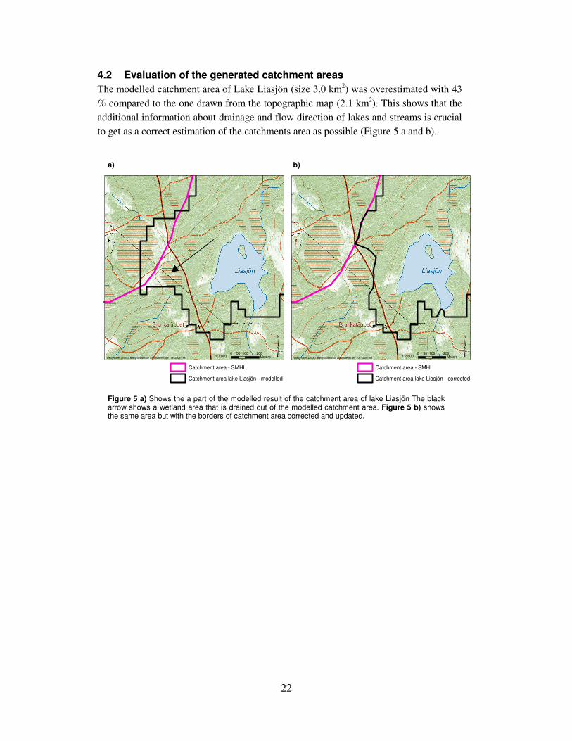
The modelled catchment area of Lake Liasjön (size 3.0 km2) was overestimated with 43

% compared to the one drawn from the topographic map (2.1 km2). This shows that the

additional information about drainage and flow direction of lakes and streams is crucial

to get as a correct estimation of the catchments area as possible (Figure 5 a and b).

Figure 5 a) Shows the a part of the modelled result of the catchment area of lake Liasjön The black arrow shows a wetland area that is drained out of the modelled catchment area. Figure 5 b) shows the same area but with the borders of catchment area corrected and updated.

0 100 20050Meters �

Catchment area - SMHI

Catchment area lake Liasjön - corrected

Viktor Kalén (2006). Bakgrundskartor Lantmäteriet dnr 106-2004/188 1:7 0000 100 20050

Meters �Catchment area - SMHI

Catchment area lake Liasjön - modelled

Viktor Kalén (2006). Bakgrundskartor Lantmäteriet dnr 106-2004/188 1:7 000

a) b)

23

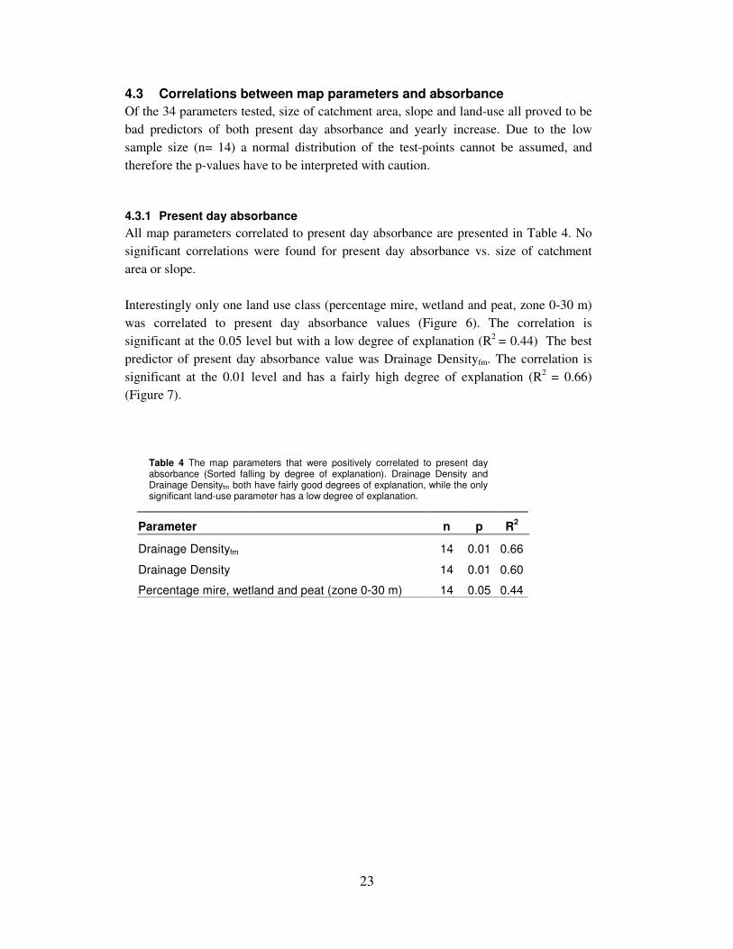
4.3 Correlations between map parameters and absorbance

Of the 34 parameters tested, size of catchment area, slope and land-use all proved to be

bad predictors of both present day absorbance and yearly increase. Due to the low

sample size (n= 14) a normal distribution of the test-points cannot be assumed, and

therefore the p-values have to be interpreted with caution.

4.3.1 Present day absorbance

All map parameters correlated to present day absorbance are presented in Table 4. No

significant correlations were found for present day absorbance vs. size of catchment

area or slope.

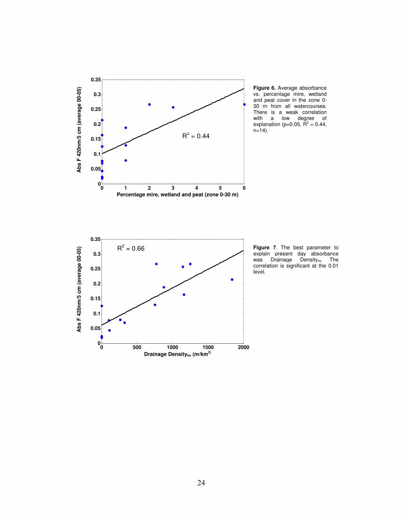
Interestingly only one land use class (percentage mire, wetland and peat, zone 0-30 m)

was correlated to present day absorbance values (Figure 6). The correlation is

significant at the 0.05 level but with a low degree of explanation (R2 = 0.44) The best

predictor of present day absorbance value was Drainage Densityfm. The correlation is

significant at the 0.01 level and has a fairly high degree of explanation (R2 = 0.66)

(Figure 7).

Parameter n p R2

Drainage Densityfm 14 0.01 0.66

Drainage Density 14 0.01 0.60

Percentage mire, wetland and peat (zone 0-30 m) 14 0.05 0.44

Table 4 The map parameters that were positively correlated to present day absorbance (Sorted falling by degree of explanation). Drainage Density and Drainage Densityfm both have fairly good degrees of explanation, while the only significant land-use parameter has a low degree of explanation.

24

Drainage Densityfm (m/km2)

Ab

s F

420n

m/5

cm

(avera

ge 0

0-0

5)

0 500 1000 1500 20000

0.05

0.1

0.15

0.2

0.25

0.3

0.35

2

R2 = 0.66 Figure 7. The best parameter to

explain present day absorbance was Drainage Densityfm The correlation is significant at the 0.01 level.

Percentage mire, wetland and peat (zone 0-30 m)

Ab

s F

420n

m/5

cm

(avera

ge 0

0-0

5)

0 1 2 3 4 5 60

0.05

0.1

0.15

0.2

0.25

0.3

0.35

Percentage mire, wetland and peat (zone 0-30 m)

R2 = 0.44

Figure 6. Average absorbance vs. percentage mire, wetland and peat cover in the zone 0-30 m from all watercourses. There is a weak correlation with a low degree of explanation (p=0.05, R

2 = 0.44,

n=14).

25

4.3.2 Yearly increase in absorbance

The significant correlations between increased absorbance and map parameters were

similar as the ones for present day absorbance. All map parameters correlated to

increase in absorbance are presented in Table 5 No significant correlations were found

for increased absorbance vs. size of catchment area or slope.

The best land–use class to predict the increase absorbance was total percentage forest

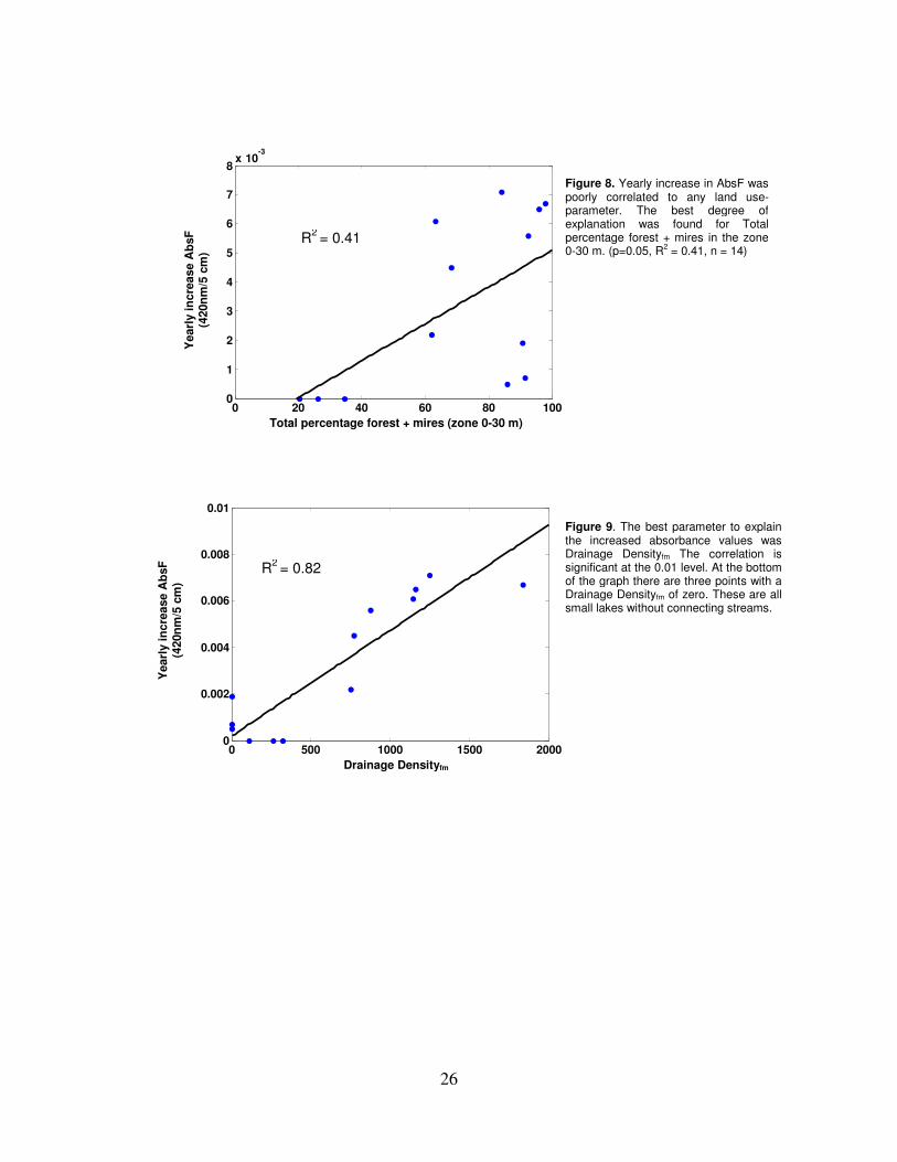
and mires (zone 0-30 m) (Figure 8). The correlation is significant at the 0.05 level, but

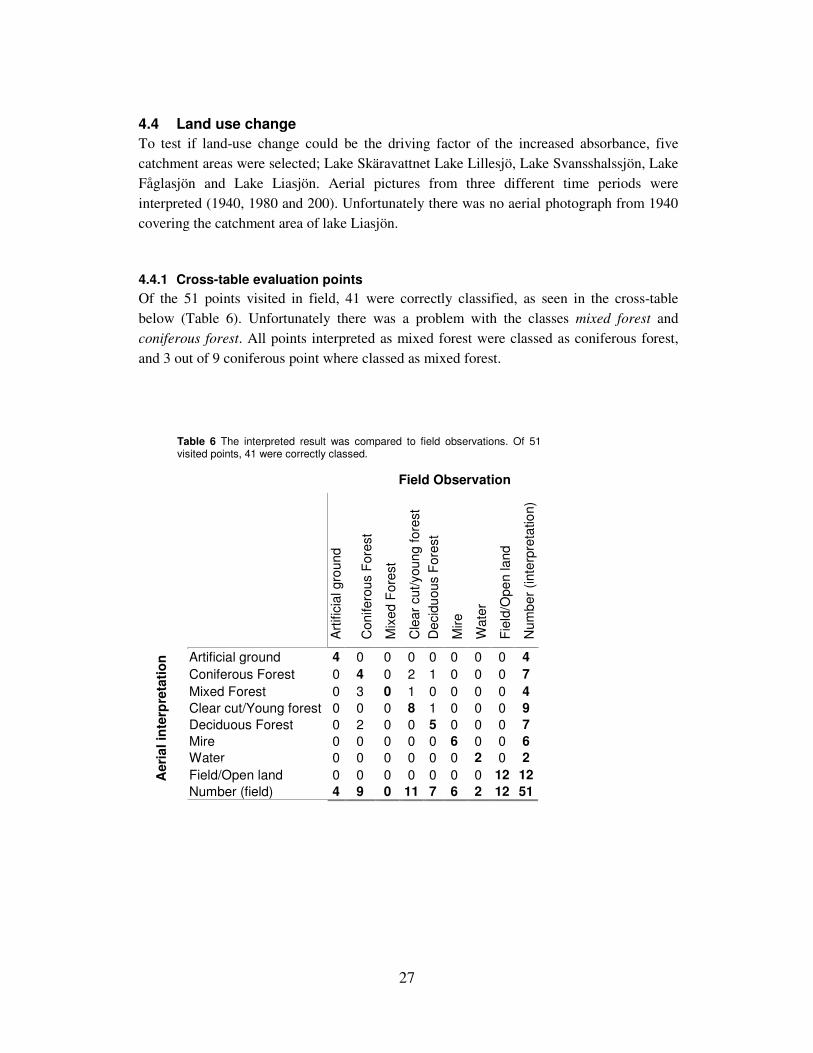
the degree of explanation is weak (R2 = 0.41). Again, Drainage Densityfm proved to be

the best predictor. The correlation is significant at the 0.01 level and the degree of

explanation is high (R2 = 0.82) (Figure 9)

Table 5 The five map parameters that were correlated to yearly increase in AbsF. Drainage Density has a very good degree of explanation, while all the land-use parameters have low degrees of explanation.

Parameter p R2

Drainage Densityfm 0.01 0.82

Drainage Density 0.01 0.52

Total percentage forest + mires (zone 0-30 m) 0.05 0.41

Total percentage forest + mires (zone 0-200 m) 0.05 0.36

Total percentage mires (including forest on mires) 0.05 0.29

26

Drainage Densityfm

Yearl

y in

cre

ase A

bsF

(4

20n

m/5

cm

)

0 500 1000 1500 20000

0.002

0.004

0.006

0.008

0.01

R2 = 0.82

Figure 9. The best parameter to explain the increased absorbance values was Drainage Densityfm The correlation is significant at the 0.01 level. At the bottom of the graph there are three points with a Drainage Densityfm of zero. These are all small lakes without connecting streams.

Total percentage forest + mires (zone 0-30 m)

Yearl

y in

cre

ase A

bsF

(4

20n

m/5

cm

)

0 20 40 60 80 1000

1

2

3

4

5

6

7

8x 10

-3

Total Percetnage forest + mires (zone 0-30 m)

R2 = 0.41

Figure 8. Yearly increase in AbsF was poorly correlated to any land use-parameter. The best degree of explanation was found for Total percentage forest + mires in the zone 0-30 m. (p=0.05, R

2 = 0.41, n = 14)

27

4.4 Land use change

To test if land-use change could be the driving factor of the increased absorbance, five

catchment areas were selected; Lake Skäravattnet Lake Lillesjö, Lake Svansshalssjön, Lake

Fåglasjön and Lake Liasjön. Aerial pictures from three different time periods were

interpreted (1940, 1980 and 200). Unfortunately there was no aerial photograph from 1940

covering the catchment area of lake Liasjön.

4.4.1 Cross-table evaluation points

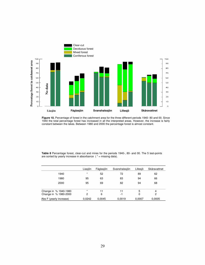
Of the 51 points visited in field, 41 were correctly classified, as seen in the cross-table

below (Table 6). Unfortunately there was a problem with the classes mixed forest and

coniferous forest. All points interpreted as mixed forest were classed as coniferous forest,

and 3 out of 9 coniferous point where classed as mixed forest.

Table 6 The interpreted result was compared to field observations. Of 51 visited points, 41 were correctly classed.

Field Observation

Aeri

al in

terp

reta

tio

n

Art

ific

ial gro

und

Conifero

us F

ore

st

Mix

ed F

ore

st

Cle

ar

cut/

youn

g fore

st

Decid

uous F

ore

st

Mire

Wate

r

Fie

ld/O

pe

n land

Num

ber

(inte

rpre

tatio

n)

Artificial ground 4 0 0 0 0 0 0 0 4

Coniferous Forest 0 4 0 2 1 0 0 0 7

Mixed Forest 0 3 0 1 0 0 0 0 4

Clear cut/Young forest 0 0 0 8 1 0 0 0 9

Deciduous Forest 0 2 0 0 5 0 0 0 7

Mire 0 0 0 0 0 6 0 0 6

Water 0 0 0 0 0 0 2 0 2

Field/Open land 0 0 0 0 0 0 0 12 12

Number (field) 4 9 0 11 7 6 2 12 51

28

Table 7 User accuracy (Ai) Producer´s accuracy (Bi) and Kappa

value for the 8 classes.

Ai Bi Kappa

Artificial ground 100 100 1,00

Coniferous Forest 57 44 0.48

Mixed Forest 0 0 0.00

Clear cut/Young forest 89 73 0.86

Deciduous Forest 71 71 0.67

Mire 100 100 1.00

Water 100 100 1.00

Field/Open land 100 100 1.00

4.4.2 Thematic accuracy

The overall agreement between the interpretation and field observation was acceptable with

a Kappa value of 0.76 (which means that the interpretation is 76 % better than if the classes

were randomly selected). Artificial ground, Mire, Water and Field/Open land all had Kappa

values of 1.00 and Clear-cut had 0.86. The land-use classes Deciduous forest and

Coniferous forest had low Kappa values, 0.67 and 0.48 respectively. Mixed forest was

lacking evaluation points and had a Kappa value of 0. This makes the interpretation

uncertain, but if all forest classes are merged to just one class, the Kappa value for that class

would be 1. Thematic accuracy is presented as User accuracy (Ai) Producer’s accuracy (Bi)

and Kappa (Table 7).

4.4.3 Land use change – interpretation of aerial photographs

The results shows that the land-use change, both looking at total percentage forest and

changes within forest classes, is small (no data where available for lake Liasjön for the

1940-period) the total percentage of forest has increased slightly between 1940-1980. The

increase is biggest for lake Fåglasjön (17 %) and smallest for lake Skäravattnet (4 %).

Between 1980-2000 there has been almost no change in total percentage forest (Figure 10

and Table 8).

Within the different forest classes there are some interesting trends. In Lake Lillesjö a large

area of mixed forest has changed to Coniferous forest. The Clear-cut areas have increased

since 1940 for lake Skäravattnet, lake Svanshalssjön and lake Lillesjö. No other clear trends

can be seen (Figure 10). Due to the low Kappa values of mixed forest and coniferous forest,

these results have to be evaluated with caution.

29

Figure 10. Percentage of forest in the catchment area for the three different periods 1940- 80 and 00. Since 1940 the total percentage forest has increased in all the interpreted areas. However, the increase is fairly constant between the lakes. Between 1980 and 2000 the percentage forest is almost constant.

Per

cen

tag

e fo

rest

in

ca

tch

men

t a

rea

Skäravattnet

Lillesjö Svanshalssjön

Fåglasjön

Liasjön

No

da

ta

Clear-cut

Deciduous forest

Mixed forest

Coniferous forest

Liasjön Fåglasjön Svanshalssjön Lillesjö Skäravattnet

1940 * 52 72 89 62

1980 95 63 83 94 66

2000 95 69 82 94 68

Change in % 1940-1980 Change in % 1980-2000

* 2

11 6

11 -1

5 0

4 2

Abs F (yearly increase) 0,0242 0,0045 0,0019 0,0007 0,0005

Table 8 Percentage forest, clear-cut and mires for the periods 1940-, 80- and 00. The 5 test-points are sorted by yearly increase in absorbance ( * = missing data).

30

4.5 Other possible explanations driving the increase in absorbance

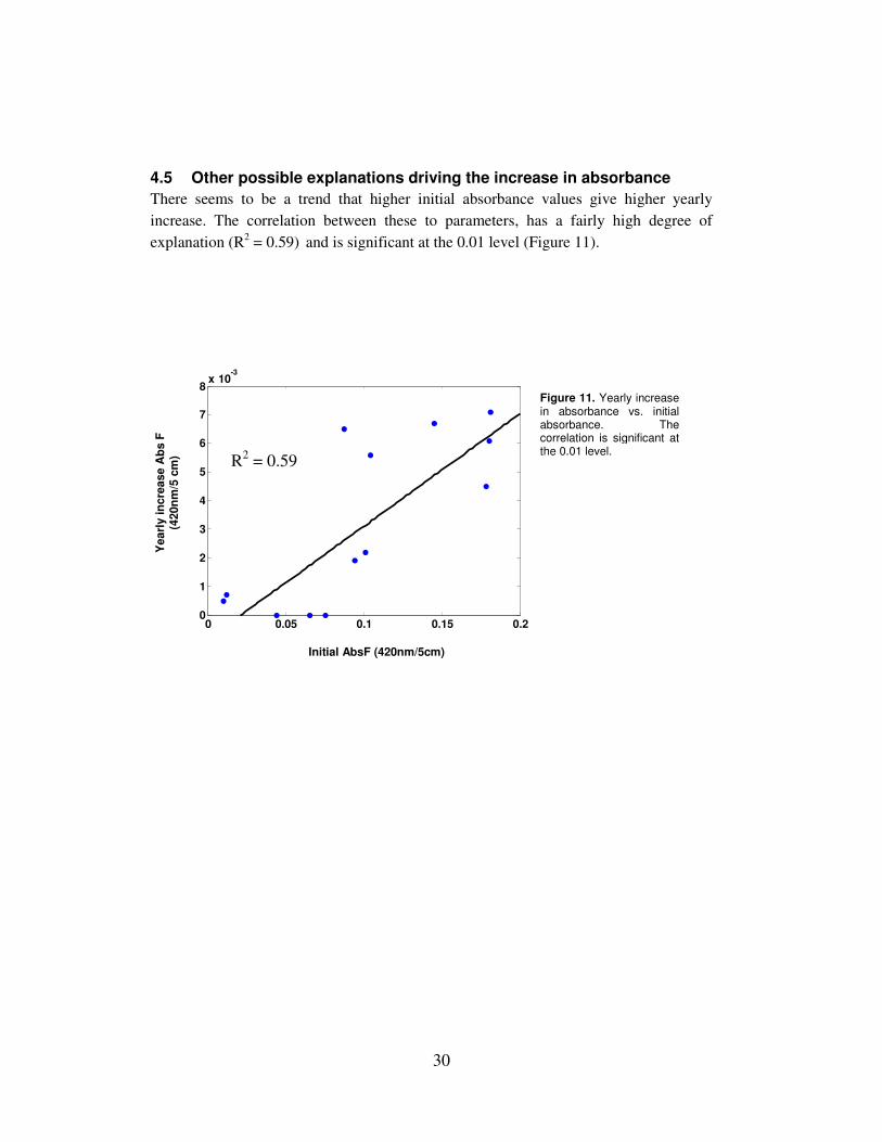
There seems to be a trend that higher initial absorbance values give higher yearly

increase. The correlation between these to parameters, has a fairly high degree of

explanation (R2 = 0.59) and is significant at the 0.01 level (Figure 11).

Initial AbsF (420nm/5cm)

Yearl

y in

cre

ase A

bs F

(4

20n

m/5

cm

)

0 0.05 0.1 0.15 0.20

1

2

3

4

5

6

7

8x 10

-3

Average absobance 1983-89

Yearl

y in

cre

ase A

bsF

420 n

m/5

cm

(1983-2

005)

R2 = 0.59

Figure 11. Yearly increase in absorbance vs. initial absorbance. The correlation is significant at the 0.01 level.

31

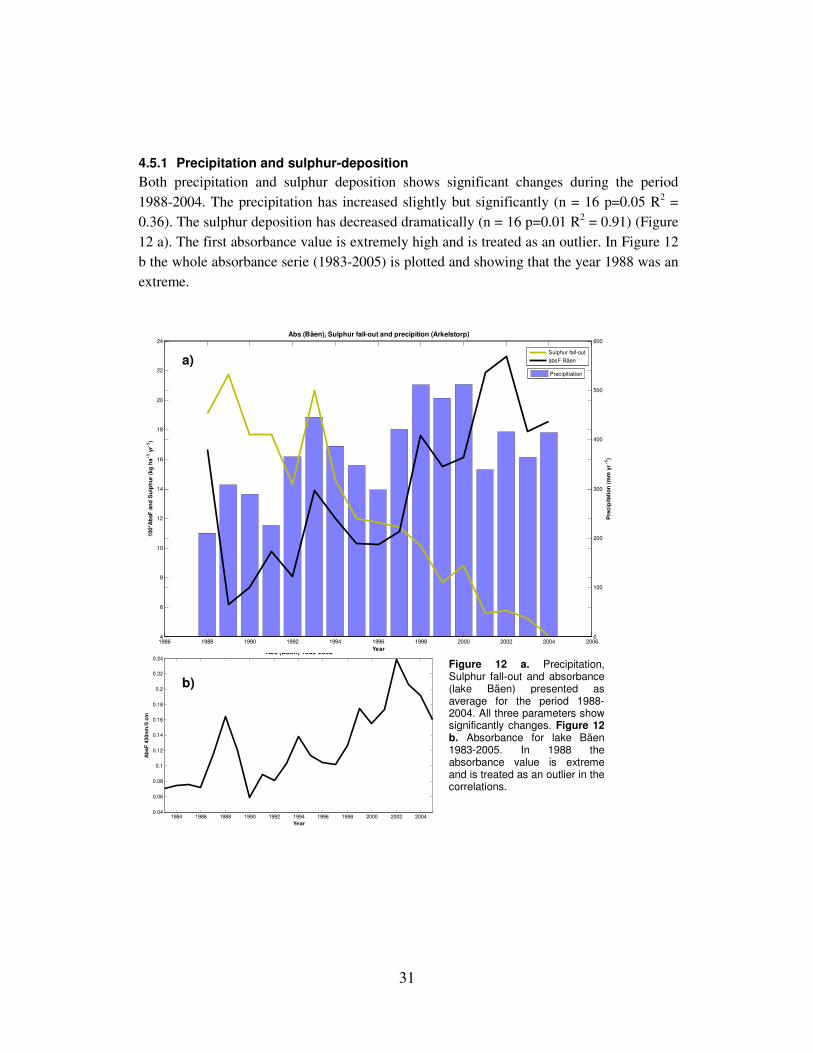
4.5.1 Precipitation and sulphur-deposition

Both precipitation and sulphur deposition shows significant changes during the period

1988-2004. The precipitation has increased slightly but significantly (n = 16 p=0.05 R2 =

0.36). The sulphur deposition has decreased dramatically (n = 16 p=0.01 R2 = 0.91) (Figure

12 a). The first absorbance value is extremely high and is treated as an outlier. In Figure 12

b the whole absorbance serie (1983-2005) is plotted and showing that the year 1988 was an

extreme.

1984 1986 1988 1990 1992 1994 1996 1998 2000 2002 20040.04

0.06

0.08

0.1

0.12

0.14

0.16

0.18

0.2

0.22

0.24 Abs (Bäen) 1983-2005

Year

Ab

sF

420n

m/5

cm

b)

1986 1988 1990 1992 1994 1996 1998 2000 2002 2004 20060

100

200

300

400

500

600

Year

Pre

cip

itati

on

(m

m y

r-1

)

4

6

8

10

12

14

16

18

20

22

24 Abs (Bäen), Sulphur fall-out and precipition (Arkelstorp)

100*A

bsF

an

d S

ulp

hu

r (k

g h

a-1

yr-1

)

Precipitiation

Sulphur fall-out

absF Bäena)

Figure 12 a. Precipitation, Sulphur fall-out and absorbance (lake Bäen) presented as average for the period 1988-2004. All three parameters show significantly changes. Figure 12 b. Absorbance for lake Bäen 1983-2005. In 1988 the absorbance value is extreme and is treated as an outlier in the correlations.

32

The correlation between absorbance and precipitation was significant at the 0.05 level. But

the degree of explanation was very low (R2 = 0.26) (Figure 13).

The correlation between absorbance and sulphur deposition was significant at the 0.01

level. The degree of explanation was better than for precipitation ( R2 = 0.62) (Figure 14).

0 5 10 15 20 250

0.05

0.1

0.15

0.2

0.25

R2 = 0.64

Sulphur fall-out (kg ha-1 yr

-1)

Ab

sF

420n

m/5

cm

lake B

äen

Figure 14. Absorbance value for Bäen (average for each year) vs. sulphur fallout (n=16)

200 300 400 500 6000.05

0.1

0.15

0.2

0.25

prec

R2 = 0.26

Precipitation (mm yr-1)

Ab

sF

420n

m/5

cm

lake B

äen

Figure 13. Absorbance value for Bäen (average for each year) was poorly correlated to yearly precipitation (n=16)

33

4.5.2 E.C.-I.R. Diagram

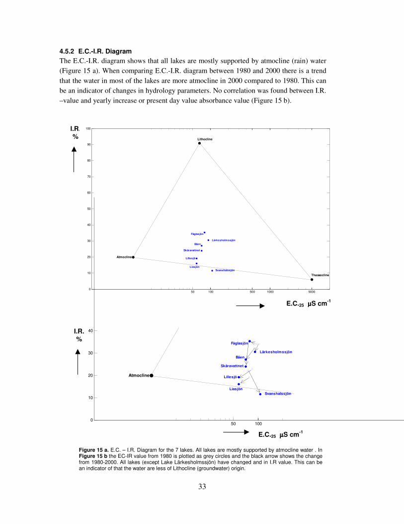
The E.C.-I.R. diagram shows that all lakes are mostly supported by atmocline (rain) water

(Figure 15 a). When comparing E.C.-I.R. diagram between 1980 and 2000 there is a trend

that the water in most of the lakes are more atmocline in 2000 compared to 1980. This can

be an indicator of changes in hydrology parameters. No correlation was found between I.R.

–value and yearly increase or present day value absorbance value (Figure 15 b).

Figure 15 a. E.C. – I.R. Diagram for the 7 lakes. All lakes are mostly supported by atmocline water . In Figure 15 b the EC-IR value from 1980 is plotted as grey circles and the black arrow shows the change from 1980-2000. All lakes (except Lake Lärkesholmssjön) have changed and in I.R value. This can be an indicator of that the water are less of Lithocline (groundwater) origin.

I.R. %

I.R. %

50 100 500 1000 50000

10

20

30

40

50

60

70

80

90

100

Atmocline

Liasjön

Bäen

Skäravattnet

Lärkesholmssjön

Svanshalssjön

Lillesjö

Fåglasjön

Thassocline

Lithocline

E.C.25 µµµµS cm-1

50 1000

10

20

30

40

Atmocline

Liasjön

Bäen

Skäravattnet

Lärkesholmssjön

Svanshalssjön

Lillesjö

Fåglasjön

E.C.25 µµµµS cm-1

34

35

5. Discussion 5.1 Absorbance values

The increase in absorbance value (~3 % per year) in the analysed data is of the same

magnitude as reported in the literature (SLU). If just looking at averages between initial and

present day values, as many as 5 out of the 15 test points are in 2000 classified as strongly

coloured, in 1980 the same number was one. According to the statistical results it is clear

that the watercolour has increased in most of the streams and lakes investigated. There is

one source of error within the statistical method used; the observations between years are

not independent and the lack of independency can affect the outcome of the correlation

(Rogers 2001).

Looking at the number of test points, n = 14 (Lake Liasjön excluded), a higher number of

observations is always desired. Since all test points (in Scania) included in the National

Environmental Survey and with a long time series were chosen this is the largest sample

size available using data from the same source and analysed in the same way. The study of

Vourenmaa et al.(2006) had a similar approach as this work and their sample size was only

n=15. For future studies, more test points can be added just looking at present day values of

absorbance and correlations to map parameters.

5.2 Map parameters

Size, Slope, and the Land-Use of a catchment area all proved to be insufficient predictors of

both the present day values and the increased absorbance values. Instead Drainage Density,

and especially Drainage Densityfm, proved to be the best predictors. These results shows

that the carbon reaching the lakes and streams originates from forest and mires, but the

water flow pathways are more important than the actual percentage forest and mires. The

higher up in soil the water flows, the higher the DOC content. This is in line with the work

of Hongve (1999) where he proposes that the effect that mires sometimes have on DOC

concentrations may depend more on their influence on water pathways than on leaching of

DOC from the peat, and that the water pathways in the catchments probably are the most

important factors determining DOC concentrations in lakes and streams. One parameter not

examined in this study that could be the interesting for future studies is the permeability of

soils. According to Hongve (1999) a higher degree of impermeable soils would give a

higher surface runoff and thus higher DOC concentrations.

The absorbance measurement is a measure of the loading of DOC. According to Kalff

(2001) the amount of DOC exported from a catchment area is highly correlated to

percentage peat and forest. The actual loading is more dependent of residence time and

water renewal times, because of removal processes such as sedimentation, microbial

decomposition and photo oxidation. This can be one explanation to the low correlations

between land-use and absorbance values recorded in this work. Drainage density can be

36

considered as a type of substitute measurement for water renewal times, because a high

drainage density probably gives a shorter residence time in a catchment area. This would

give yet another explanation to why Drainage Density was such a god predictor of

watercolour.

Due to the small sample size (n=14) the test-points cannot be assumed to be normal

distributed. This gives a high uncertainty when evaluating the p-values. For future studies

better statistical methods were the data is tested for normal distribution is preferred.

Another approach would be to add more test points so that normal distribution can be

assumed (n > 30). Probably, the correlations for land-use parameters are not normal

distributed, this in combination with the bad R2 values and the high p-values (p close to

0.05) shows that land-use parameters not can explain the observed absorbance values.

5.3 Land-use change

As the parameter Land-Use proved to be an insufficient predictor of present day absorbance

values as well as increase in absorbance. This must lead to the conclusion that a change in

land-use from open land/cultivated land to forest does not necessarily give higher increase

in absorbance values. As can be seen in Figure 8 there are catchment areas with a high

percentage forest and mires, but still a very small increase in absorbance value. However,

the total percentage forest has increased in all interpreted areas. Of the 4 lakes interpreted,

the two with the highest yearly increase in absorbance (lake Fågasjön and Lake

Svanshalssjön) also have the biggest increase in total percentage forest between 1940-2000.

The increase in forest has probably increased the total carbon content in the catchments,

and can well contribute to a small part of the increase in watercolour. But that it would be

the driving factor is very unlikely. The fact that between 1980 and 2000 there has been

almost no change strengthens this theory. Larger changes in land-use and a stronger

relationship between present day absorbance and percentage forest is required to explain the

observed increase in watercolour. This study just focused on percentage changes in land-

use, not were the land-use took place. On interesting thing for future studies would be to

look at land-use changes close to streams, if a forest were planted close to a stream, the

parameter Drainage Densityfm would increase.

The changes within forest classes are rather small. The catchment of lake Lillesjö is the one

that experienced the largest change between forest classes; ~35 % mixed forest had become

(mostly) coniferous forest. This is a change that could contribute to an increase in

absorbance value, but the absorbance increase in Lake Lillesjö is very small. Due to the low

thematic accuracy of mixed forest and coniferous forest, comparisons between different

forest classes have to be made carefully. However, there are explanations to the low

accuracy values. The number of evaluation points is small and not evenly distributed

between classes. The reason for this is the time/cost of being in field and the fact that

several points that were planned to be visited were unreachable due to closed roads.

Another source of error is due to limitation- and scale problems. Looking at an aerial

37

photography, one area can be classed as mixed forest, but when the evaluation point is

visited in field there is a chance that there is only coniferous forest surrounding the point.

This problem can be overcome with better field preparations and stricter definitions of sizes

of objects. These two explanations point to that the interpretations of mixed forest and

coniferous forest probably are better than the thematic accuracy values expresses.

5.4 Other explanations driving the increase

Instead the driving increase seems to be o f a more widespread phenomenon. Evans et al.

(2004) found a strong positive correlation (R2 = 0.7) between the rate of annual DOC

increase and initial DOC concentrations. Due to this they argued that mean DOC release

per unit of soil organic carbon had increased, which implies a driving mechanism operating

at a large scale. Vourenmaa et al. (2006) also reported on a correlation between annual

TOC change and average present day values of absorbance. The results from this work also

show a correlation between yearly increase and initial absorbance value, although a bit

weaker (R2 = 0.59, p = 0.01). Since lakes and streams with a high initial absorbance value

increases the most, the driving factor seems to accelerate an already existing processes.

The correlations between sulphur deposition, precipitation and absorbance values are just to

be seen as a brief guidance to what can be the driving factor behind the increasing

absorbance values. Just looking at lake Bäen, both precipitation and sulphur deposition

have changed and both of them correlate to absorbance value for Lake Bäen, therefore it is

possible that both of these can have influenced the amount of DOC exported to the lake.

The facts that sulphur deposition has the highest degree of explanation, that it is working on

a large scale, and that the deposition has decreased dramatically in Sweden during the

examined period (SLU 2007) all points to that this could be what drives the increase in

watercolour. When comparing data in this way, it is important to remember that a strong

linear relationship does not necessarily imply that there is a causal connection between the

two variables (Rogersson 2001). More data and statistical analysis are required to be able to

sort out and determine what drives the increase.

An interesting thing to investigate would be changes in precipitation patterns. It can be so

that there are more dry periods followed by more heavily rainfall. In this more water would

flow higher up in the soil layers due to saturated soils (Hope et al. 1994). The results from

the E.C-I.R. diagram can be an indicator of this. The water seems to be more of atmocline

origin, which means that either the amount of atmocline water has increases, or the amount

of groundwater decreases. According to SGU (2007) no big trends of changes in

groundwater level have been recorder in Scania during the examined period. Instead

changes in the amount of precipitation and/or precipitation pattern could be an explanation

to the changes in the E.C.- I.R. diagram.

38

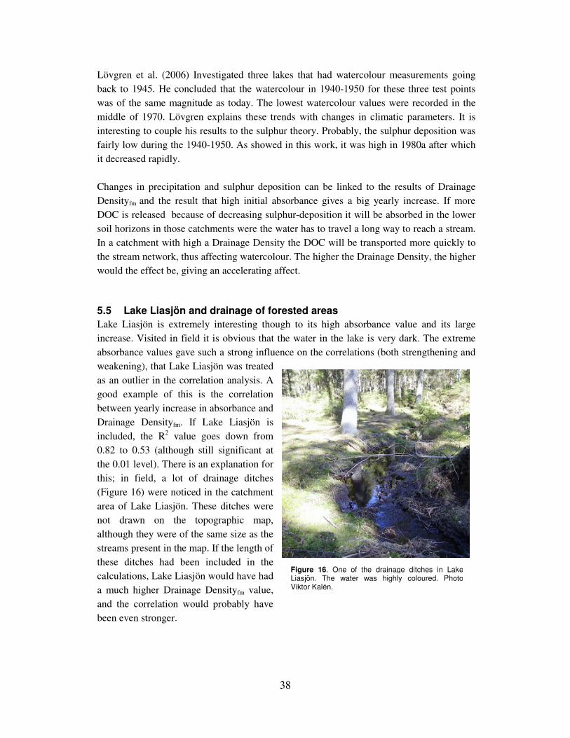
Figure 16. One of the drainage ditches in Lake Liasjön. The water was highly coloured. Photo Viktor Kalén.

Lövgren et al. (2006) Investigated three lakes that had watercolour measurements going

back to 1945. He concluded that the watercolour in 1940-1950 for these three test points

was of the same magnitude as today. The lowest watercolour values were recorded in the

middle of 1970. Lövgren explains these trends with changes in climatic parameters. It is

interesting to couple his results to the sulphur theory. Probably, the sulphur deposition was

fairly low during the 1940-1950. As showed in this work, it was high in 1980a after which

it decreased rapidly.

Changes in precipitation and sulphur deposition can be linked to the results of Drainage

Densityfm and the result that high initial absorbance gives a big yearly increase. If more

DOC is released because of decreasing sulphur-deposition it will be absorbed in the lower

soil horizons in those catchments were the water has to travel a long way to reach a stream.

In a catchment with high a Drainage Density the DOC will be transported more quickly to

the stream network, thus affecting watercolour. The higher the Drainage Density, the higher

would the effect be, giving an accelerating affect.

5.5 Lake Liasjön and drainage of forested areas

Lake Liasjön is extremely interesting though to its high absorbance value and its large

increase. Visited in field it is obvious that the water in the lake is very dark. The extreme

absorbance values gave such a strong influence on the correlations (both strengthening and

weakening), that Lake Liasjön was treated

as an outlier in the correlation analysis. A

good example of this is the correlation

between yearly increase in absorbance and

Drainage Densityfm. If Lake Liasjön is

included, the R2 value goes down from

0.82 to 0.53 (although still significant at

the 0.01 level). There is an explanation for

this; in field, a lot of drainage ditches

(Figure 16) were noticed in the catchment

area of Lake Liasjön. These ditches were

not drawn on the topographic map,

although they were of the same size as the

streams present in the map. If the length of

these ditches had been included in the

calculations, Lake Liasjön would have had

a much higher Drainage Densityfm value,

and the correlation would probably have

been even stronger.

39

Another observation made in the catchment area of Lake Liasjön was that the soil had sunk.

It looked like many of the trees were “standing on their on roots”. The explanation to this

can be that the drainage ditches has lowered the water table. When the water table is

lowered, the soil is oxygenated which will enhances the microbial activity and increase the

breakdown in soil (Wallace 2006). Most likely this leads to an increase in the amount of

DOC exported. The effect would probably be the same if already existing ditches were

made deeper or wider. Recently a study where made at the County administrative Board of

Scania. The study aimed to control if a number drainage ditches in Scania were according

to the depth and width that the duty allows. The results show that the majority of the

drainage ditches examined where either to deep, to wide or both to deep and wide according

to what the duty allows (Grosen 2007, unpublished data). This can well contribute to a

higher leakage of DOC to the water systems. Because of this and because of the

correlations between Drainage Densityfm and watercolour it is of great interest to discuss

how the drainage of forested areas will be done in the future. This also raises the question if

increased drainage can be the driving factor of the watercolour? This is most unlikely since

this factor is not working on a large scale, and due to the fact that since 1986 there is a

prohibition against drainage in Scania. Although exemption can be given, it is not likely

that the drainage have increased enough to explain the observed trends and being the

driving factor behind the increased watercolour.

5.6 What will happen in the future?

According to literature, approximately 1-5 % of NPP is returned to the atmosphere as CO2

by evasion of DOC in lakes and streams. Since the concentration of DOC is regulating the

rate of CO2 evaded (Vetenskapsrådet), an increase in DOC also means an increase in CO2

emission. According to Dillon and Mollot (1994) the net annual accumulation of carbon

based on NEP may be overestimated because of export of carbon to lakes and streams.

The main issue concerning DOC trends is whether it will continue increase, stabilize or

return to lower values. If sulphur is the driving factor it could be so that what is observed is

a flushing effect. During the acidification the DOC particles have been bound up, and is

now flushed trough the water systems. If so, the absorbance values can return to more

acceptable values, but since DOC still is more easily leached compared to when sulphur

deposition was high the water colour will not go back to the values experienced in the

1980s. Other things that can keep the watercolour at a high level is increases/changes in

precipitation due to climate change. e.g. storm events gives significant changes in flow

paths and makes water float higher up in the soil layers (Hope et al. 1994). According to

SMHI ( Rossby Center SMHI 2007) there will be an increase in both precipitation and

extreme precipitation in Scania of ~ 5 to 10 % during the two next decades. If decreased

sulphur deposition is the explanation to the increased watercolour, this would lead to a very

interesting conclusion; by solving the environmental problem of acidification, another

problem appears.

40

6. Conclusions

• The increase in watercolour for the data used in this work is of the same magnitude

as reported in literature.

• Generating catchment areas just using ArcGIS and a DEM (resolution 50*50 m) is

not a sufficient method. If an as good results as possible is desired the location and

flow direction of streams, wetlands and lakes has to be taken into account. Instead,

the modelling should be viewed as a very helpful tool, especially if many

catchment areas are to be generated.

• Drainage Densityfm proved to be the map parameter best explaining both present

day values and increased absorbance values. Land-use proved to be an insufficient

parameter explaining absorbance values.

• Land-use change can most likely not be the driving factor behind the increased

watercolour.

• Decreased sulphur deposition tends to be the driving factor behind the increased

absorbance values. But increased precipitation and/or changes in precipitation

pattern can also be an explanation.

Acknowledgements I want to thank my supervisor Harry Lankreijer for help and discussions during the way. I also want to thank Anna Broström for help and supervision. At the County Administrative Board of Scania there are many people who helped me, and I am very grateful that I got the opportunity to do my thesis at the County Administrative Board of Scania. Especially I want to thank Lars Collvin for all help and interesting and enthusiastic discussions. Anna Hagerberg for nice drawings and discussions. I also want to thank Marie Eriksson for all help, I’ve learned a lot! Thanks to Vibeke Lirås for giving me the original idea to this thesis! I want to thank the IT/GIS division for technical help. Thanks to Marie Sager and Verena Maichel for great cooperation (Marie, I wont mention anything about maps…).

I want to thank my family for supporting me during my University years. Finally I want to thank my girlfriend for helping me with splelling problems, for discussion and new ideas, and for always being there.

41

7. References Articles

Bishop, K., Pettersson, C., Alard, B., Lee, Y-H. (1994). Identification of the riparian

sources of aquatic dissolved organic carbon. Environmental International , 20(1), pp.

11-19

Cronan, C.S., Aiken, G.R, (1984). Chemistry and transport of soluble humic substances

in forested watersheds of the Adirondack Park, New York Geoehimica et

Gosmochimica .&a Vol. 49, pp. 1697-1705

Dahlström, N., (2005). Function and dynamics of woody debris in boreal forest streams.

Doctoral Thesis, Umeå University, Umeå, 21 pp

Dillon, P.J and Molot, L.A., (1997). Dissolved Organic and Inorganic Carbon Mass

Balances in Central Ontario Lakes. Biogeochemistry, Vol. 36, No. 1, Dissolved

Organic Carbon as an Integration of Global Stresses on Freshwater., pp. 29-42.

Edwards NT, Shugart HH Jr, McLaughlin SB, Harris WF & Reichle DE., (1981). Carbon

metabolism in terrestrial ecosystems. In: Reichle DE (Ed) Dynamic properties of

ecosystems (pp 499-536). Cambridge University Press, New York

Evans,C. D., Chapman, P. J., Clark, J.M., Monteith, D.T., Cresser, M.S., (2006).

Alternative explanations for rising dissolved organic carbon export from organic soils.

Global Change Biology 12 (11), pp. 2044–2053.

Evans, C.D., Monteithb, D.T., Cooper D.M., (2004). Long-term increases in surface

Water dissolved organic carbon: Observations, possible causes and environmental

impacts, Environmental Pollution 137., pp. 55-71

Hope, D., Billet, M.F., Cresser, M.S., (1994). A review of the export of carbon in river

water: fluxes and processes. Environmental Pollution 84. pp. 301-324

Hongve, D., (1999) Production of dissolved organic carbon in forested catchments.

Journal of Hydrology 224, pp. 91–99

Jonsson, A., Algesten, G., Bergström, A.-K., Bishop, K., Sobek, S., Tranvik. L.J. and

Jansson, M., (2006). Integrating aquatic carbon fluxes in a boreal catchment carbon

budget. Journal of Hydrology 334: 141-150.

Lövgren, S., Forsenius, M., Andersen, T. (2003), Climate induced water colour increase

In Nordic lakes and streams due to humus. Nordic Council of Ministres, Brochure (12

pp)

Neal, C., Robson, A.l., Neal, M., Reynolds, B., (2005) Dissolved organic carbon for

upland acidic and acid sensitive catchments in mid-Wales. Journal of Hydrology 304

(2005) pp 203–220

Roulet, N., Moore , T.R., (2006). Browning the waters. NATURE 444, pp. 283-284.

Sachse, A., Henrion, R., Gelbrecht, J., Steinberg, C.E.W. (2005),. Classification of

Dissolved organic carbon (DOC) in river system: Influence of catchment

characteristics and autochthonous processes, Organic Geochemistry 36 (2005), s.

923–935

Sibelle, I., Biological stability in drinking water distribution systems: a review, Année

Biole 78. pp. 117-161

Temnerud, J., Spatial Variation of Dissolved Organic Carbon Along Streams in

Swedish Boreal Cathcments. Örebro University, University Libraries, 2005,

42

www.ub.oru.se

Van Wirdum, G. (1980). Simple description of water quality changes during a hydrological cycle for use in nature protection. In: Hooghart JC (Ed). Wayer quality in groundwater systems. Report nr 5. Commission of hydrological research TNO, Den Haag, The Netherlands (In Dutch)

Vuorenmaa, J., Forsius,M., Mannio, J., (2006). Increasing trends of total organic carbon

concentrations in small forest lakes in Finland from 1987 to 2003, Science of the

Total Environment 365 47–65

Wallace, Z.E., Holden, J., McDonald, A.T., (2006). Drain blocking: An effective

Treatment for reducing dissolved organic carbon loss and water discolouration in a

drained peatland, Science of the total environment 367 (2006), pp. 811-821

Worrall, F., Burt, T.P., Adamson, J., (2006). The rate of and controls upon DOC loss in

a peat catchment, Journal of Hydrology 321, s. 311–325

Whittaker RH, Likens GE, Bormann FH, Eaton JS & Siccama TG (1979) The Hubbard

Brook ecosystem study: forest nutrient cycling and element behaviour. Ecol. 60. pp.

203-220

Books Brönnmark, C.,Hansson, L-A., (2005), The Biology of Lakes and Ponds, Second

Edition,Oxford University Press Inc., New York, pp

Eklundh, L., (2000), Geografisk informationsbehandling, Metoder och tillämpningar.

Stockholm, Byggforskningsrådet: pp. 348

Grootjans, A.B., (1985), Changes of groundwater regime in wet meadows. Casparie Heerhugowaard b.v., pp. 146

Findlay, E.G., Sinsabaugh, R.L., 2003, Aquatic Ecosystems Interactivity of Dissolved

Organic Matter. Academic Press, pp 512

Janssen, L. F. L., and Huurneman, C. G., (2001), Principles of remote sensing. The

international Institute for aerospace survey and earth sciences (ITC),

Netherlands, pp. 410 Kalff, J., (2002), Limnology: inland water ecosystems, Prentice-Hall, Inc, pp. 592

Rogersson, A.R., (2001), Statistical methods for Geography. SAGE Publications LTD.,

pp. 236

Thurman, E.M., (1985), Organic Geochemistry of Natural Waters. Martin Nijhoff/Dr W

junk Publishers, Dordrecht., pp. 497

Internet sources SLU a., Article downloaded from http://www.slu.se/?id=965&puff=13 (downloaded 2007-05-

30) SLU b.,Water chemistry data downloaded from

http://info1.ma.slu.se/ma/www_ma.acgi$Project?ID=StationsList&P=All – (downloaded 2007-04-27)

Rossby Center SMHI 2007., Climate data http://www.smhi.se/cmp/jsp/polopoly.jsp?d=8785&l=sv -downloaded 2007-06-17

Personal Communication

SGU (2007). Thunholm, B.,

43

Reports Naturvårdsverket. Bedömningsgrunder för miljökvalitet. Sjöar och vattendrag. Rapport

4913.

Lantmäteriet - Svenska CORINE Marktäckedata Produktspecifikation

Dokumentnummer SCMD-0001 2002.

LUSTRA-programmet 2001-2002 (www-lustra.slu.se/rapportermm/pdf/2002.pdf)

SLU 2007, Miljötrender Nr 2, pp 11

Vetenskapsrådet: Omsättning och effekter av humusämnen i sjöar, vattendrag och

Havsområden - abstracts

Used data Svenska Marktäckedata SMD Vektor. Version 2.2 (2002-06-03) LMV LMV Fastighetskartan Hydrografi Linje 2006 – LMV GSD LMV Fastighetskartan 2003 Sjöar – LMV GSD LMV GSD-Höjddata

Topographic map, Economic map © Bakgrundskartor Lantmäteriet, dnr 106-2004/188

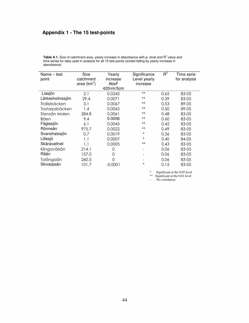
44

Appendix 1 - The 15 test-points

Name – test point

Size catchment area (km

2)

Yearly increase

AbsF 420nm/5cm

Significance Level yearly

increase

R2 Time serie

for analysis

Liasjön 2.1 0.0242 ** 0.65 83-05 Lärkesholmssjön 29.4 0.0071 ** 0.39 83-05 Trollebäcken 3.1 0.0067 ** 0.53 89-05 Tostarpsbäcken 1.4 0.0065 ** 0.50 89-05 Stensån Malen 284.8 0.0061 ** 0.48 83-05 Bäen 9.4 0.0056 ** 0.60 83-05 Fåglasjön 6.1 0.0045 ** 0.42 83-05 Rönneån 975.7 0.0022 ** 0.49 83-05 Svanshalssjön 0.7 0.0019 * 0.36 83-05 Lillesjö 1.1 0.0007 * 0.40 84-05 Skäravattnet 1.1 0.0005 ** 0.43 83-05 Klingavälsån 214.1 0 - 0.06 83-05 Råån 157.0 0 - 0.06 83-05

Tolångaån 260.5 0 - 0.06 83-05 Skivarpsån 101.7 -0.0001 * 0.15 83-05

Table A 1. Size of catchment area, yearly increase in absorbance with p- level and R2 value and

time series for data used in analysis for all 15 test points (sorted falling by yearly increase in absorbance)

* Significant at the 0.05 level ** Significant at the 0.01 level - No correlation

45

Appendix 2 - Aerial pictures

Picture name Number of GCP:s

Polynom RMS Error

Georeferenced by:

Svanshalssjön 814_04210_44 53 2nd 4.1 This project

Liasjön 814_04129_46 59 2nd 3.8 This project

Lillesjö 244_03268_28 20 3rd 5.6 This project

Skärvattnet 844_03480_05 45 2nd 4.5 This project

Fåglasjön 3C40_21 39 2nd 9.5 Andersson, 2004

Table A 2. The 5 interpreted aerial pictures, number of GCPs, polynomial and RMS value for georeferencing.

46

Lunds Universitets Naturgeografiska institution. Seminarieuppsatser. Uppsatserna finns tillgängliga på Naturgeografiska institutionens bibliotek, Sölvegatan 12, 223 62 LUND. Serie startade 1985. The reports are available at the Geo-Library, Department of Physical Geography, University of Lund, Sölvegatan 12, S-223 62 Lund, Sweden. Report series started 1985. 79. Ullman, M., (2001): El Niño Southern Oscillation och dess atmosfäriska

fjärrpåverkan. 80. Andersson, A., (2001): The wind climate of northwestern Europe in SWECLIM

regional climate scenarios. 81. Lalloo, D., (2001): Geografiska informationssystem för studier av polyaromatiska

kolväten (PAH) – Undersökning av djupvariation i BO01-området, Västra hamnen, Malmö, samt utveckling av en matematisk formel för beräkning av PAH-koncentrationer från ett kontinuerligt utsläpp.

82. Almqvist, J., Fergéus, J., (2001): GIS-implementation in Sri Lanka. Part 1: GIS-applications in Hambantota district Sri Lanka : a case study. Part 2: GIS in socio-economic planning : a case study.

83. Berntsson, A., (2001): Modellering av reflektans från ett sockerbetsbestånd med hjälp av en strålningsmodell.

84. Umegård, J., (2001): Arctic aerosol and long-range transport. 85. Rosenberg, R., (2002): Tetratermmodellering och regressionsanalyser mellan

topografi, tetraterm och tillväxt hos sitkagran och lärk – en studie i norra Island. 86. Håkansson, J., Kjörling, A., (2002): Uppskattning av mängden kol i trädform – en

metodstudie. 87. Arvidsson, H., (2002): Coastal parallel sediment transport on the SE Australian

inner shelf – A study of barrier morphodynamics. 88. Bemark, M., (2002): Köphultssjöns tillstånd och omgivningens påverkan. 89. Dahlberg, I., (2002): Rödlistade kärlväxter i Göteborgs innerstad – temporal och

rumslig analys av rödlistade kärlväxter i Göteborgs artdataarkiv, ADA. 90. Poussart, J-N., (2002): Verification of Soil Carbon Sequestration - Uncertainties

of Assessment Methods. 91. Jakubaschk, C., (2002): Acacia senegal, Soil Organic Carbon and Nitrogen

Contents: A Study in North Kordofan, Sudan. 92. Lindqvist, S., (2002): Skattning av kväve i gran med hjälp av fjärranalys.

93. Göthe, A., (2002): Översvämningskartering av Vombs ängar. 94. Lööv, A., (2002): Igenväxning av Köphultasjö – bakomliggande orsaker och

processer. 95. Axelsson, H., (2003): Sårbarhetskartering av bekämpningsmedels läckage till

grundvattnet – Tillämpat på vattenskyddsområdet Ignaberga-Hässleholm. 96. Hedberg, M., Jönsson, L., (2003): Geografiska Informationssystem på Internet –

En webbaserad GIS-applikation med kalknings- och försurningsinformation för Kronobergs län.

97. Svensson, J., (2003): Wind Throw Damages on Forests – Frequency and Associated Pressure Patterns 1961-1990 and in a Future Climate Scenario.

47

98. Stroh, E., (2003): Analys av fiskrättsförhållandena i Stockholms skärgård i relation till känsliga områden samt fysisk störning.

99. Bäckstrand, K., (2004): The dynamics of non-methane hydrocarbons and other trace gas fluxes on a subarctic mire in northern Sweden.

100. Hahn, K., (2004): Termohalin cirkulation i Nordatlanten. 101. Lina Möllerström (2004): Modelling soil temperature & soil water availability in

semi-arid Sudan: validation and testing. 102. Setterby, Y., (2004): Igenväxande hagmarkers förekomst och tillstånd i Västra

Götaland. 103. Edlundh, L., (2004): Utveckling av en metodik för att med hjälp av lagerföljdsdata

och geografiska informationssystem (GIS) modellera och rekonstruera våtmarker i Skåne.

104. Schubert, P., (2004): Cultivation potential in Hambantota district, Sri Lanka 105. Brage, T., (2004): Kvalitetskontroll av servicedatabasen Sisyla 106. Sjöström., M., (2004): Investigating Vegetation Changes in the African Sahel

1982-2002: A Comparative Analysis Using Landsat, MODIS and AVHRR Remote Sensing Data

107. Danilovic, A., Stenqvist, M., (2004): Naturlig föryngring av skog 108. Materia, S., (2004): Forests acting as a carbon source: analysis of two possible

causes for Norunda forest site 109. Hinderson, T., (2004): Analysing environmental change in semi-arid areas in

Kordofan, Sudan 110. Andersson, J., (2004): Skånska småvatten nu och då - jämförelse mellan 1940,

1980 och 2000-talet 111. Tränk, L., (2005): Kadmium i skånska vattendrag – en metodstudie i

föroreningsmodellering. 112. Nilsson, E., Svensson, A.-K., (2005): Agro-Ecological Assessment of Phonxay

District, Luang Phrabang Province, Lao PDR. A Minor Field Study. 113. Svensson, S., (2005): Snowcover dynamics and plant phenology extraction using

digital camera images and its relation to CO2 fluxes at Stordalen mire, Northern Sweden.

114. Barth, P. von., (2005): Småvatten då och nu. En förändringsstudie av småvatten och deras kväveretentionsförmåga.

115. Areskoug, M., (2005): Planering av dagsutflykter på Island med nätverkanalys 116. Lund, M., (2005): Winter dynamics of the greenhouse gas exchange in a natural

bog. 117. Persson, E., (2005): Effect of leaf optical properties on remote sensing of leaf area

index in deciduous forest. 118. Mjöfors, K., (2005): How does elevated atmospheric CO2 concentration affect

vegetation productivity? 119. Tollebäck, E.,(2005): Modellering av kväveavskiljningen under fyra år i en anlagd

våtmark på Lilla Böslid, Halland 120. Isacsson, C., (2005): Empiriska samband mellan fältdata och satellitdata – för

olika bokskogområden i södra Sverige. 121. Bergström, D., Malmros, C., (2005): Finding potential sites for small-scale Hydro

Power in Uganda: a step to assist the rural electrification by the use of GIS

48

122. Magnusson, A., (2005): Kartering av skogsskador hos bok och ek i södra Sverige med hjälp av satellitdata.

123. Levallius, J., (2005): Green roofs on municipal buildings in Lund – Modeling potential environmenta benefits.

124. Florén, K., Olsson, M., (2006): Glacifluviala avlagrings- och erosionsformer I sydöstra Skåne – en sedimentologisk och geomorfologisk undersökning.

125. Liljewalch-Fogelmark, K., (2006): Tågbuller i Skåne – befolkningens exponering. 126.

Irminger Street, T., (2006): The effects of landscape configuration on species richness and diversity in semi-natural grasslands on Öland – a preliminary study.

127. Karlberg, H., (2006): Vegetationsinventering med rumsligt högupplösande satellitdata – en studie av QuickBirddata för kartläggning av gräsmark och konnektivitet i landskapet.

128 Malmgren, A., (2006): Stormskador. En fjärranalytisk studie av stormen Gudruns skogsskador och dess orsaker.

129 Olofsson, J., (2006): Effects of human land-use on the global carbon cycle during the last 6000 years.

130 Johansson , T., (2006): Uppskattning av nettoprimärproduktionen (NPP) i stormfällen efter stormen Gudrun med hjälp av satellitdata.

131 Eckeskog, M., (2006) Spatial distribution of hydraulic conductivity in the Rio Sucio drainage basin, Nicaragua.

132 Lagerstedt, J., (2006): The effects of managed ruminants grazing on the global carbon cycle and greenhouse gas forcing.

133 Persson, P., (2007) Investigating the Impact of Ground Reflectance on Satellite Estimates of Forest Leaf Area Index

134 Valoczi, P. (2007) Koldioxidbalans och koldioxidinnehållsimulering av barrskog I Kristianstads län, samt klimatförändringens inverkan på skogen.

135 Johansson, H. (2007) Dalby Söderskog - en studie av trädarternas sammansättning 1921 jämfört med 2005