Introduction Analog to digital (A/D) data conversion, simply put, entails the measurement of a quantity from

a device with the value being directly input to the computer, and stored as digital information.

With the advent of the modern age of computers, this is a more and more popular route for the

acquisition of data in a Kinesiology laboratory, where it often has replaced the traditional

method of pen and paper recording of data and subsequent typed entry into a computer. In

addition to facilitating quick and accurate entry of information, it also affords new opportunities

for data collection that were impossible using older forms of acquisition. An example is a

skinfold caliper fitted with a potentiometer as discussed in the next chapter. However, a word

of warning in the use of analog/digital data collection, one must always be wary of potentially

unnoticed error appearing because of the computerization of so many functions. With the

various forms of signal conditioning available, both analog and digital, it is often possible to

introduce error into your data by incorrect application of procedures such as amplification,

smoothing etc. Too much emphasis cannot be put on trying to understand your signal and data

analysis. One must always be checking to see that the results make sense, and that you fully

understand the ramifications of any signal conditioning.

The intention in this and the subsequent chapters in this section is to give you an

understanding of the basic processes involved in A/D conversion, to use EXCEL to give some

experience in several forms of digital signal conditioning and to understand the potential for

A/D conversion in the realm of Kinesiology.

Analog Signals

Outside of the computer we tend to be dealing with analog signals. Commonly we have a

voltage as our signal coming from an electrode or transducer. This analog signal is a

continuous waveform that has a value at every point in time. In a physics lab you will have

seen analog signals displayed on oscilloscopes, or in a kinesiology lab when a chart recorder

depicts the ECG picked up by electrodes. Computers, although powered by voltages do not

operate on analog information. Information must be in the form of binary numbers, referred to

as digital information.

chapter 3-1 Analog to Digital Data Conversion Basics

3-1.2 Analog to Digital Data Conversion Basics

When a device is producing a signal that we wish to bring into a computer to analyze, that

signal needs to be changed from the analog form into digital information. Analog to digital data

conversion is achieved by having a device attached to your computer called an A/D board

(with associated software), which will sample the analog signal at discrete points in time and

store this as digital information.

Digital Information

The digits 0 to 9 have different meanings based upon their position within the number. The

digit to the right represents the number of 1s, the next digit to the left the number of 10s. This

decimal system is simply a coding convention that is used for numbers as depicted in Figure

3-1.1.

The number 2543 therefore means 2 one

thousands, 5 one hundreds, 4 tens and 3 ones.

Notice also the decimal coding of the base of 10

to incrementing powers. Computers do not work

on the decimal system, but rather code

information in terms of open or closed circuits

i.e., binary information. There are two states,

open or closed, which can mean yes or no, high

or low, but in computer terms, the two states get coded as 1 or 0. Numbers therefore need to

be represented in the binary system not our commonly used decimal system.

Figure 3-1.2 shows how the decimal number 41

can be converted into binary notation. Notice

that the difference between the two notations is

that in the decimal system the base of 10 is

raised by incrementing powers and in the

binary system the base of 2 is raised by

incrementing powers. First find the highest

power of 2 that will go into 41 once. 25 is 32, 26

is 64, so the largest power is 25 and therefore receives the 1 code. 41 – 32 = 9, so 24 (16) will

not go into it, hence the 0 code. The next power of 2 to go into the remainder once is 23 (8)

leaving a remainder of 1. Only 20 (1) will go into the remainder 1 so the decimal number 41 is

coded in binary as 101001.

The term BIT of information is a contraction of BINARY DIGIT. Although you can only code a

binary state i.e. 0 = high, 1 = low or 0 = yes, 1 = no, more than one bit can code more

information. When two bits are used for coding there are 22 = 4 possible combinations of two

1’s or 0’s, resulting in 4 states 00, 01, 10 and 11. Early computers were set up with blocks of 8

DECIMAL – Base of 10

2543 1000 100 10 1

103 102 101 100 2 5 4 3

Figure 3-1.1: Decimal coding system

BINARY – Base of 2

41 32 16 8 4 2 1

25 24 23 22 21 20 1 0 1 0 0 1

Figure 3-1.2: Binary coding system

Measurement & Inquiry in Kinesiology 3-1.3

bits of memory called bytes. A byte or 8 bits can code 28 or 256 possible combination of eight

1’s and 0’s. The American Standard Code for Information Interchange is a coding system

using 8 bits to code 256 commonly used characters. For example an A is coded as 01000001.

Files of information are often sent in ASCII code which can be read by almost all application

software.

Modern computers store information in multiples

of Kilobytes, Megabytes and Gigabytes (Table

3-1.1). A Kilobyte (KB) is 210 bytes which is

1,024 bytes. Interestingly, the decimal prefixes

we are used to, were attached to the binary

multiples of bytes. Although in decimal terms it

sounds like a Kilobyte should be 1,000 bytes,

because it is 210 it is only close to 1,000. A

Megabyte is not a million bytes but 220 or

1,048,576 bytes, and a Gigabyte is not 1,000,000,000 but 230 or 1,073,741,824 bytes.

Modulation

In order to move digital information from one site to another, computer files can be stored on

some form of memory medium such as CDs or DVDs. However, we can also directly link two

computers to send information. Digital

information can be coded into a high

frequency analog signal carried by cable

between computers. An analog waveform

has three basic characteristics: Amplitude,

Frequency and Phase. Digital information

can be coded into these high frequency

carrier waves by alternating from one state of

the characteristic to another, in a process

called modulation.

Modulation involves changing from one state

of a characteristic to a second for a finite

time periods to encode either 1’s or 0’s

respectively. Figure 3-1.3 illustrates Frequency Modulation, as two levels of frequency are

used to encode the 1’s and 0’s. Also shown is Amplitude Modulation where two levels of

amplitude are used to the same end.

Bit Binary Digit

Byte 8 Bits, 28 or 256 combinations

ASCII American Standard Code for Information Interchange e.g. A = 01000001

Kilobyte (KB) 210 = 1024 bytes

Megabyte (MB) 220 = 1,048,576 bytes

Gigabyte (GB) 230 = 1,073,741,824 bytes

Table 3-1.1: Definitions of the quantities of digital information

Figure 3-1.3: Frequency and amplitude modulation

3-1.4 Analog to Digital Data Conversion Basics

You will probably be more familiar with these terms by their abbreviations FM and AM on your

radio dial, which represent Frequency modulation and Amplitude Modulation, respectively. A

third less popular modulation is by having two phases of the signal representing the 1’s and 0’s

and is called Phase Modulation. When information leaves your computer a piece of hardware

is required to modulate the digital information onto the carrier signal. At the target computer the

signal needs to be demodulated as the information encoded in the carrier signal is taken into

the computer. This gives rise to the name of the piece of hardware you may be familiar with, a

MODEM (MOdulation-DEModulation).

Components Required for A/D Conversion

Our focus in this section of the text however, is not how computers can transmit information

one to another, but how we can bring an analog signal into the computer in digital form. There

are certain basic components necessary for analog to digital data conversion which will be

expanded upon in this and subsequent chapters.

• Analog signal from an electrode or transducer: Having identified the quantity to be

measured, which may be anything from a length to a pressure or temperature, there

needs to be an analog signal in the form of a voltage, where the magnitude of the

voltage reflects the magnitude of the measured quantity. This could be a naturally

occurring voltage sensed by electrodes such as E.M.G. or E.E.G., or more commonly

a voltage produced by a transducer turning the measurement into a voltage (e.g.

potentiometer, force transducer). Transducers and electrodes are called sensing

elements, that are the link between the recording equipment and the event being

monitored.

• Analog conditioning: It is often necessary to manipulate the signal while it is still a

voltage in the cable, in order to minimize noise or to begin the quantification of the

phenomenon. Such manipulation in called Analog Conditioning and includes

processes such as amplification, integration and filtering, by custom built electronic

circuits.

• A/D Board & Software: In order to enter the computer the signal must be changed

from the continuous analog signal into the discrete digital data used in computers. This

means that the analog signal (voltage) must be sampled at discrete points in time. This

is called A/D conversion and is the task of the A/D board in conjunction with the

controlling software.

The rest of this chapter and subsequent chapters in this section are devoted to providing some

detail to the components listed above.

Analog Signal from Electrodes

Measurement & Inquiry in Kinesiology 3-1.5

Electrodes transform ionic currents into electrical voltage that can be amplified and passed on

to the recording equipment. Electrodes can be required to receive information from many or

single cells. The electrodes needed to measure the activity of a large number of cells need to

have low impedance, and they should be relatively large in size. Large size picks up activity

from many cells; and since activity or current is coming from many cells, if its magnitude is

large, one can manage with small impedance. An example, is that electrodes to record

surface EMG, EEG and EKG are generally 0.5 – 1.0 cm in diameter. To record from single

cells, one uses very small electrodes (small recording area). Because of the small recording

area these electrodes have a high resistance and hence, small currents from single cells

produce recordable voltages (V=IR). Since they have a high resistance, they also pick up any

stray noise; one has to minimize this noise without affecting the signal. One way of eliminating

noise is to have a good ground on the subject or the animal preparation. The second one is to

do differential recording (see differential amplifiers below). To record intracellularly from within

cells or for patch clamp recordings, one deals with extremely high resistance electrodes.

There are many kinds of electrodes used to detect biophysical signals, but two factors affecting

all types are: electrode artefact and electrical safety. We will not address electrical safety here

other than to say that extreme care must be taken to ensure that the system is correctly set up

to ensure the safety of the subject. Electrode artefact is a problem that can render your data

useless, thus it is a very important factor to consider and hopefully to minimize. The type of

artefact from electrodes can be either electrochemical; physical or biological in origin.

Electrode Artefacts

• Physical: Movement of the tissue relative to the electrode can cause cause distortion

of the signal. Careful cleaning and mild abrasion of the skin can reduce skin

impedance and reduce error generated by electrode movement

• Electrochemical: A reaction between the tissue and the metal of the electrode can

produce a charge gradient known as the electrode double layer. This can cause error

to be introduced into the signal. For example, electrodes to record surface EMG, EEG

and EKG are generally made up of Silver – Silver Chloride. Silver is a good conductor

and chloriding it prevents it from chemically reacting with the biological tissue. When it

reacts with the biological tissue, its properties change, in fact it is not a good conductor

anymore.

• Biological: Other signals in the body may be picked up as well. For instance, E.M.G.

may be pickup during E.C.G. signal collection. Details of this and other issues related

to E.M.G. will be discussed in chapter 3-4.

•

3-1.6 Analog to Digital Data Conversion Basics Analog Signal from Transducers

If the body is not producing a bioelectric signal that can be sensed with electrodes then the

voltage needs to be produced by a tranducer. A transducer is a device that transforms one

form of energy into another. Tranducers may be of many forms, they provide an electrical

output proportional to the event being measured. Many transducers are some form of resistive

element where the resistance changes in relation to the quantity being monitored.

Potentiometers (variable resistances) are popular transducers finding applications in linear

measurement and electrogoniometer devices. In chapter 3-3 we will make use of a rotary

potentiometer to provide a voltage from a spring operated skinfold caliper. Calibration is a very

important issue with all transducers, in order to transforrm voltage into real values of the

measured quantity. The method used for calibration of the skinfold caliper potentiometer will

also be discussed in chapter 3-3.

A form of transducer you typically find in a Kinesiology lab would be a strain gauge. Strain

gauges are the most common transducers for measuring force. A strain gauge consists of a

wire whose resistance is proportional to its length. If a strain gauge is mounted on a metal

plate, which is fixed at one length, and then a force is applied to bend the other end of the

plate, the length of the plate changes. Since the strain gauge is attached to the plate it too

changes the length (L) of the strain gauge. If L changes to L+ΔL, the resistance changes to

R+ΔR. If a current was passing through the strain gauge, the original voltage drop V will

change to V+ΔV. One can calibrate ΔV in terms of applied force, then during experiments we

observe ΔV, and from our calibration curves we can find out how much force was applied.

Strain gauges typify the basic features of a transducer; they produce a voltage and it needs

calibrating.

There are some basic general requirements for a good transducer:

• Sensitivity and range: Sensitivity refers to the smallest change in the measured

quantity that can be detected by a transducer. The sensitivity required often depends

upon the situation. If you have a linear displacement transducer, does it need to be

sensitive to 0.0001mm or will 0.01mm be satisfactory? The answer would dictate your

choice of transducer. The transducer also needs to have enough range to deal with

measured values. Loss of information may happen if the range of the transducer is not

great enough, and bottoming out or clipping occurs.

• Linearity: Ideally, there is a linear relationship between the input and output of the

transducer. This will result in easier calibrations. Often however, a transducer will not

be linear over its full range and so a calibration curve is required.

Measurement & Inquiry in Kinesiology 3-1.7

• Response time: This is how fast the transducer responds to changes in input. If the

inputs change faster than the time constant of the transducer, the output is distorted

because it never reaches the maximum steady-state value.

Analog Conditioning

For many different reasons the analog signal may not be in a form that you desire. While it is

still a voltage in the cable it can be modified by custom electronic circuitry to modify the signal.

This is referred to as analog conditioning. We will be dealing with some basic forms of analog

conditioning in this text, particularly with reference to electromyography (E.M.G.) in chapter 3-

4. Conditioning really means doing something to change the signal in an appropriate manner

to modify the output to achieve a certain goal. If the modifications are not appropriate or unduly

change the representation of the underlying phenomenon this would be regarded as distortion

rather than conditioning. Two common examples of analog conditioning are amplification and

filtering.

Amplification: If the range of a signal is small in comparison to the range of the A/D board it

must be amplified. By example, E.M.G. signal amplitude can range from 0 to 6 millivolts (peak-

to-peak), whereas the A/D board may have a range from -10 to +10 volts. The E.M.G. signal

needs to be amplified to make better use of this full range.

Filtering: A very important and popular form of conditioning is filtering. The basic aim is to

modify the signal by removing certain frequencies. This is achieved by passing the signal

through a custom built filtering circuit.

A/D Board

A piece of hardware called an “Analog to Digital data conversion board (A/D board)” is

necessary in order to sample the analog signal. This board may have many input channels to

allow for the monitoring of various devices simultaneously. Its job is to sample the analog

signal (voltage) at discrete points in time, assign a digital code to that sampling and save it in

digital memory.

Two important characteristics of an A/D converter are its resolution and sampling rate.

Resolution is defined as a measure of the smallest amplitude value as a percent of full scale to

which a quantity can be determined. In other words how finely it can discriminate values of the

incoming signal. The sampling rate will determine how faithfully the shape of the incoming

signal is reproduced.

Sampling Rate & Aliasing

The continuous analog signal is turned into discrete data points by the A/D board and

3-1.8 Analog to Digital Data Conversion Basics

accompanying software, by sampling at a fixed frequency (Figure 3-1.4). The data are

sampled every h seconds and this digitized value stored in memory on the computer. The

ideal situation would be to pick a very small value for h, so as to lose as little information as

possible in the digitization process. The A/D board characteristics impose limits on how small h

can be. However, sampling is

inefficient if h is too small and

unnecessary information is

stored. The task is to find the

optimum size for h. A sampling

interval of h sec gives a

sampling rate of 1/h samples

per sec or h Hz. For example, if

we sample with h set at 0.01

seconds then the frequency of

sampling is 1/0.01 samples per

second or 100 Hz.

The signal needs to be sampled

at a rate at least twice as

frequent as the highest

frequency in the single (Nyquist

rule). Such a frequency is called

the Nyquist frequency or folding

frequency and is given by:

hf N 2

1=

Where fN is the Nyquist frequency and h is the sampling interval in seconds

The word folding here implies

that high frequencies are folded

back into low frequencies. Use of the Nyquist rule guards against aliasing, where an alias is

the resultant signal when the sampling rate is two slow and the resultant signal looks very

different than the original analog signal being sampled (figure 3-1.5).

Figure 3-1.5 shows that if the h picked is too large, then aliasing will result in the amount of

high frequencies will be reduced and the amount of lower frequencies will be increased. The

sampling frequency is also the highest frequency that the resultant data can be analyzed at.

TimeVoltage

Figure 3-1.4: Digitization of an analog signal (black line).

Sampling at a fixed frequency produces the digitized signal (red

dots).

Time

Voltage

Figure 3-1.5: Aliasing: higher frequency analog signal (black line) misrepresented as a very low frequency digitized signal (red dots), due to sampling at too low a frequency.

Measurement & Inquiry in Kinesiology 3-1.9

For example if you sample at 100Hz then when you analyze the resultant digital data there will

be no frequencies present over 100Hz, even if they had been in the original analog signal.

Determining the sampling rate is a key issue as you try to minimize the amount of digitized

information, without compromising the content of the digitized information in comparison to the

original analog signal.

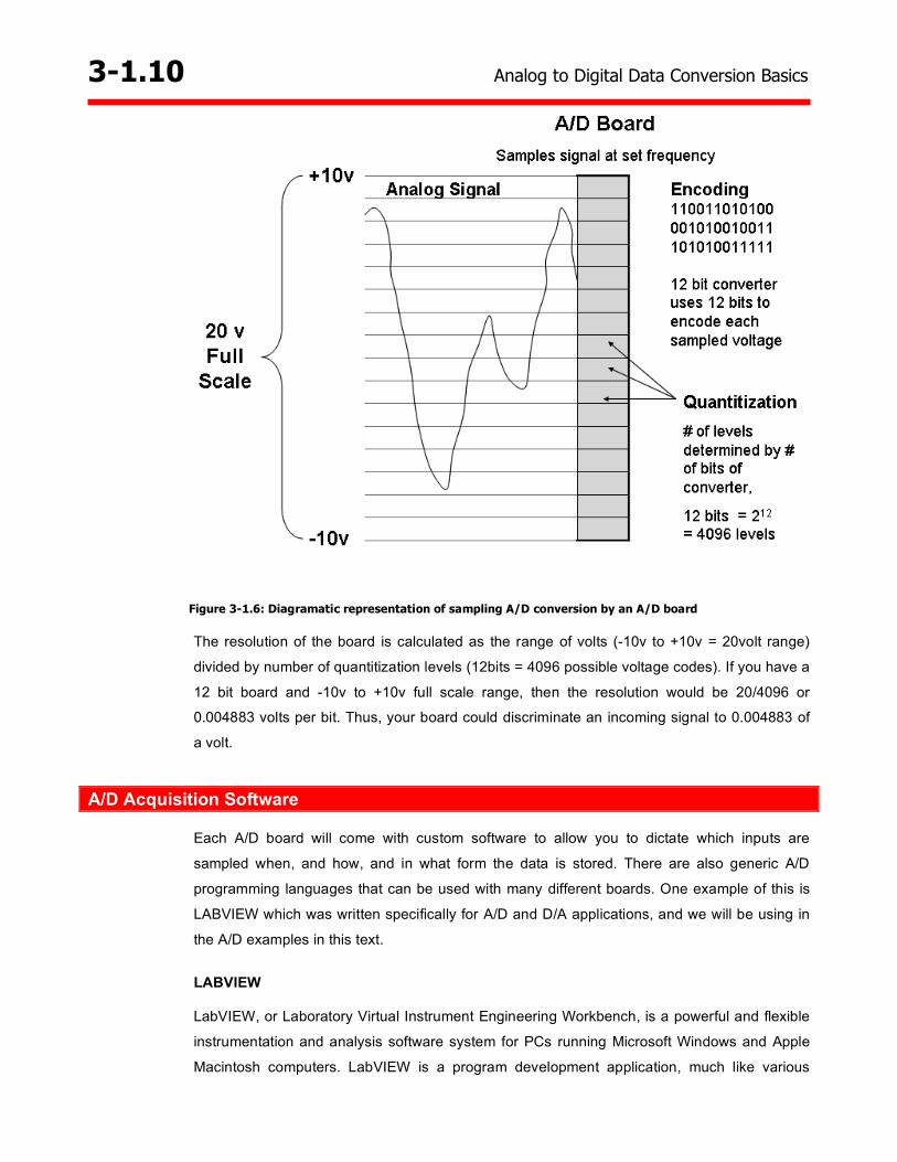
Resolution of an A/D Converter

Resolution is defined as a measure of the smallest amplitude value as a percent of full scale to

which a quantity can be determined. It is important that the A/D board used can adequately

discriminate the incoming signal. The calculation of the resolution is based upon the range of

voltage that the board can deal with and then how many different digital codes it can assign to

the sampled values. Quantitization is the process of sampling the incoming voltage into a given

number of voltage levels with encoding being the assigning of a digital code to each of those

voltage levels. Figure 3-1.6 is a diagrammatic representation of the process.

Quantization and Encoding by the A/D Board

Any given board uses a certain number of bits to encode the sampled voltages. 12-bit boards

using 12 bits or a 12 binary digit number (e.g. 110101110001) to encode any sampled voltage,

are in common use. There are 212 (4096) possible combinations of 1s and 0s in 12 bits,

therefore 4096 different levels of voltage could be encoded with a 12 bit board. The more bits

your board uses then the more levels of voltage can be encoded.

Full Scale of the A/D Board

The board will have a range of voltages that it can respond to (-5v to +5v; -10v to +10v etc.).

This is important in determining the resolution of the board and is termed the full scale range of

the board. Data will be lost if the incoming signal is higher or lower than this full scale range. It

is important therefore to know the possible voltage range of incoming signals so as to use as

much of the full scale range as possible without going outside the limits. In E.M.G. the millivolt

signal is amplified up to a number of volts to make best use of A/D boards which tend to have

-5v to +5v or -10v to +10v full scale range. This will optimize the use of the resolution of the

A/D board.

3-1.10 Analog to Digital Data Conversion Basics

Figure 3-1.6: Diagramatic representation of sampling A/D conversion by an A/D board

The resolution of the board is calculated as the range of volts (-10v to +10v = 20volt range)

divided by number of quantitization levels (12bits = 4096 possible voltage codes). If you have a

12 bit board and -10v to +10v full scale range, then the resolution would be 20/4096 or

0.004883 volts per bit. Thus, your board could discriminate an incoming signal to 0.004883 of

a volt.

A/D Acquisition Software

Each A/D board will come with custom software to allow you to dictate which inputs are

sampled when, and how, and in what form the data is stored. There are also generic A/D

programming languages that can be used with many different boards. One example of this is

LABVIEW which was written specifically for A/D and D/A applications, and we will be using in

the A/D examples in this text.

LABVIEW

LabVIEW, or Laboratory Virtual Instrument Engineering Workbench, is a powerful and flexible

instrumentation and analysis software system for PCs running Microsoft Windows and Apple

Macintosh computers. LabVIEW is a program development application, much like various

Measurement & Inquiry in Kinesiology 3-1.11

commercial C or BASIC development systems. There are many forms of programming

language as described below.

Machine Language: This is the fundamental programming language of the central processing unit (C.P.U.) of the computer.

Assembly Language: A low level language (meaning specific to one type of C.P.U.) that has abbreviations representing several steps in machine language.

High-Level Languages: High level languages are not specific to one type of C.P.U. Examples of these are COBOL, FORTRAN, PASCAL, C, BASIC. They have varying degrees of readability in that they have text representing operations.

Macro Languages: Applications software such as EXCEL have macros which are the ability to preprogram spreadsheeting steps

Visual Programming Languages: With the advent of the Graphical User Interface (G.U.I.) programming languages changed whereby there were a library of prewritten visual objects. The code did not therefore have to be written from scratch for every image that appeared in your program. Examples of this are Visual Basic and LABVIEW

While high level programming languages are text-based to create lines of code, LabVIEW uses

a graphical programming language, G, to create programs in a flowchart-like form called a

block diagram, eliminating a lot of the syntactical details. LabVIEW programs are called virtual

instruments (Vls) because their appearance and operation imitate actual instruments.

However, behind the scenes they are analogous to main programs, functions, and subroutines

from popular programming languages like C or BASIC. Fgure 3-1.7 shows the LabVIEW user

interface for the E.M.G. VI used in chapter 3-4. Figure 3-1.8 shows the code behind it.

Figure 3-1.7: Front panel of the E.M.G. acquisition LabVIEW VI

Figure 3-1.8: Block diagram of the E.M.G. acquisition LabVIEW VI

The interactive user interface of the VI is called the frontpanel, so named because it simulates

the panel of a physical instrument. The front panel can contain knobs, push buttons, graphs,

and many other controls (user inputs) and indicators (program outputs). You input data using a

mouse and keyboard, and then view the results produced by your program on the screen. The

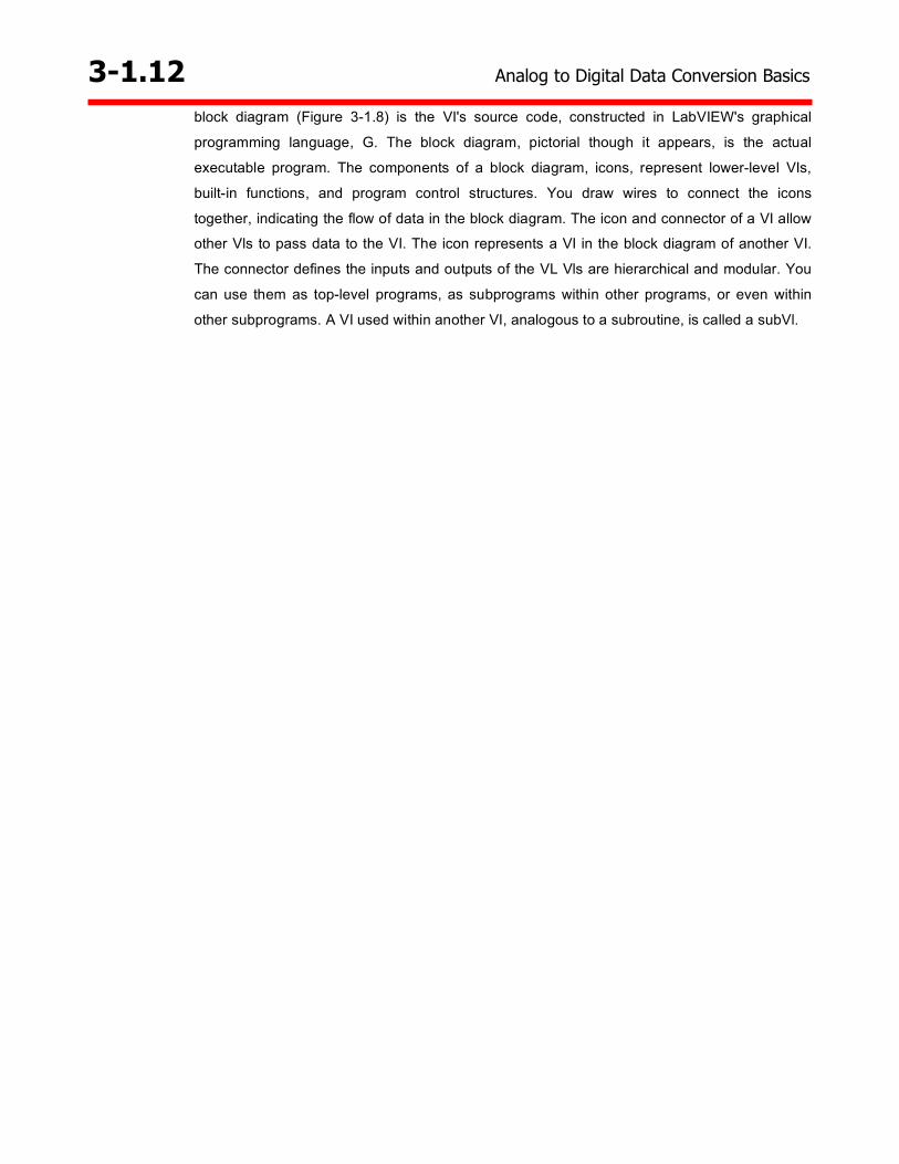
3-1.12 Analog to Digital Data Conversion Basics

block diagram (Figure 3-1.8) is the VI's source code, constructed in LabVIEW's graphical

programming language, G. The block diagram, pictorial though it appears, is the actual

executable program. The components of a block diagram, icons, represent lower-level VIs,

built-in functions, and program control structures. You draw wires to connect the icons

together, indicating the flow of data in the block diagram. The icon and connector of a VI allow

other Vls to pass data to the VI. The icon represents a VI in the block diagram of another VI.

The connector defines the inputs and outputs of the VL Vls are hierarchical and modular. You

can use them as top-level programs, as subprograms within other programs, or even within

other subprograms. A VI used within another VI, analogous to a subroutine, is called a subVl.