ANALISIS TRIWULANAN: Perkembangan Moneter, Perbankan dan ... … · ANALISIS TRIWULANAN:...
107
Transcript of ANALISIS TRIWULANAN: Perkembangan Moneter, Perbankan dan ... … · ANALISIS TRIWULANAN:...

1ANALISIS TRIWULANAN: Perkembangan Moneter, Perbankan dan Sistem Pembayaran, Triwulan II - 2007
BULLETIN OF MONETARY ECONOMICS AND BANKING
Center for Central Banking Research and EducationBank Indonesia
PatronDewan Gubernur Bank Indonesia
Board of Editor
Prof. Dr. Anwar NasutionProf. Dr. Miranda S. Goeltom
Prof. Dr. InsukindroProf. Dr. Iwan Jaya Azis
Prof. Iftekhar HasanProf. Dr. Masaaki Komatsu
Dr. M. SyamsuddinDr. Perry Warjiyo
Dr. Iskandar Simorangkir Dr. Solikin M. JuhroDr. Haris Munandar
Dr. Andi M. Alfian ParewangiDr. M. Edhie Purnawan
Dr. Burhanuddin AbdullahDr. Andi M. Alfian Parewangi
Editorial Chairman
Dr. Perry Warjiyo
Managing EditorDr. Darsono
Dr. Siti AstiyahDr. Andi M. Alfian Parewangi
SecretariatIr. Triatmo Doriyanto, M.S
Nurhemi, S.E., M.ATri Subandoro, S.E
This bulletin is published by Bank Indonesia, Center for Central Banking Research and Education. Contents and results research in the writings in this bulletin entirely the responsibility of the authors and not an official view of Bank Indonesia.
We invite all parties to write in this bulletin paper delivered in the form files to Center for Central Banking Research and Education, Bank Indonesia, Tower Sjafruddin Prawiranegara Floor 21; Jl. M.H. Thamrin No. 2, Central Jakarta, email: [email protected].
The Bulletin is published quarterly in April, July, October and January, for who wish to obtain this publication can contact the Dissemination Unit - Dissemination Division Statistics and Management Intern, Department of Statistics, Bank Indonesia, Tower Sjafruddin Prawiranegara floor 2; Jl. M.H. Thamrin No. 2, Central Jakarta, tel. (021) 2981-8206. For request subscribe: tel. (021) 2981-6571, fax. (021) 3501912.

Quarterly Outlook on Monetary, Banking, and Payment System In Indonesia:
Quarter II, 2015
TM. Arief Machmud, Syachman Perdymer, Muslimin Anwar, Nurkholisoh Ibnu Aman, Tri
Kurnia Ayu K, Anggita Cinditya Mutiara K, Illinia Ayudhia Riyadi
The Role of Macroprudential Policy to Control Exchange Rate Volatility,
Liquidity, and Bank Credit
Muhammad Edhie Purnawan, M. Abd. Nasir
The Market Structure of The Bank, Its Performance, and The Macroprudential Policy
Tumpak Silalahi, Adler H.Manurung, Yuli Teguh Hidayat
The Impact of Exchange Rate Misalignment on Safeguards Policy of ASEAN-5
Dila Vindayani, Dedi Budiman Hakim, Alla Asmara
The Branch Expansion and The Performance of The Banks: The Case of Indonesia
Hery Prasetyo, Sony Sunaryo
BULLETIN of moNETary EcoNomIcsaNd BaNkINg
Volume 18, Number 1, July 2015
21
59
1
43
81

This page intentionally left blank
1Quarterly Outlook on Monetary, Banking, and Payment System In Indonesia: Quarter II, 2015
QUARTERLY OUTLOOK ONMONETARY, BANKING, AND PAYMENT SYSTEM IN
INDONESIA: QUARTER II, 2015
TM. Arief Machmud, Syachman Perdymer, Muslimin Anwar, Nurkholisoh Ibnu Aman, Tri Kurnia Ayu K,
Anggita Cinditya Mutiara K, Illinia Ayudhia Riyadi1
1 Authors are researcher on Monetary and Economic Policy Department (DKEM). TM_Arief Machmud ([email protected]); Syachman Perdymer ([email protected]); Muslimin Anwar ([email protected]); Nurkholisoh Ibnu Aman ([email protected]); Tri Kurnia Ayu K ([email protected]); Anggita Cinditya Mutiara K ([email protected]); Illinia Ayudhia Riyadi ([email protected])
This paper provides current analysis of the ongoing quarter, and the brief outlook on the forthcoming
quarter. We use a field survey along with estimation of macroeconomic models to provide the assessment
and to make some projections on the monetary, the banking, and the payment system in Indonesia. This
paper confirms the slowdown of the Indonesian economy during quarter two 2015 due to the slowing
investment and the government expenditure, and the weak export performance. With the fiscal stimulus
launched by the government, we expect to see an improvement in next two quarters. The lower current
account deficit and manageable inflation will help to maintain the macroeconomic stability; however, the
high global uncertainty will put depreciation pressure on Rupiah.
Abstract
Keywords: macroeconomy, monetary, economic outlook.
JEL Classification: C53, E66, F01, F41

2 Bulletin of Monetary, Economics and Banking, Volume 18, Number 1, July 2015
I. GLobaL DEVELoPMENT
Global economic growth is expected to be slower than previously expected, amid risk in global financial markets remains high. The slowdown was mainly due to the US economic growth is not as high as previously expected and the Chinese economy is still slowing. Although the FOMC in July 2015 a little more optimistic about the economic recovery, generally the US economy in 2015 is estimated to be lower than previous forecast, driven by the realization that US economic growth in the first quarter and the second in 2015 a relatively low due to the weak investment on non-residential sector. Correspondingly, the uncertainty of interest rate hikes Fed Funds Rate (FFR) in the US is continuing. Meanwhile, the European economy is expected to improve, supported by stronger domestic demand associated with the decrease in the unemployment rate. Moreover, the pressure on Greece also eased after receipt of the general requirements of the bailout fund by the state parliament. In contrast, the Chinese economy is still weak amid its stock market pressure continues. To maintain the competitiveness of exports, the Central Bank of China devalued the Yuan and changes the Yuan exchange rate determination mechanism to be more market-driven, which also provides additional impacts the risk of exchange rate pressure on countries trading partners of China, including Indonesia. The world economy is generally expected to slow impact on international commodity prices are still declining. On the other hand, the global financial markets still face high risks associated with the uncertainty of interest rate hikes in the US FFR and policy adjustments to the Yuan exchange rate.
US economic growth is not as high as predicted earlier predictions. The lower growth in the US economy driven by lower realization of US economic growth in the first and second quarter of the original estimate. Realization of US economic growth in the first and second quarter lower than expected affected by lower investment, associated with weak non-residential investment (Figure 1). In addition, economic indicators from both the demand and supply have not shown solid improvements. The US economic recovery on the demand side is still limited, reflected in the improvement of the level of retail sales were slightly restrained. On the production side, industrial production and capacity utilization is still in a downward trend.
European economy is expected to improve. Such improvement is underpinned by stronger domestic demand, reflected in the growth in total retail sales increased (Figure 2). The increase in domestic demand is also consistent with the improvement in the labor sector. This was reflected in the unemployment rate in some countries, notably Germany, Italy, Spain, and Ireland. Expectations of economic recovery of Europe increased in line with the rebound in oil prices, the easing of geopolitical tension, and effective QE policy. Meanwhile, the pressure on Greece also eased after receipt of the general requirements of the bailout fund by the state parliament.

3Quarterly Outlook on Monetary, Banking, and Payment System In Indonesia: Quarter II, 2015
Figure 1. US Growth Component
Figure 2. European Retail Sales
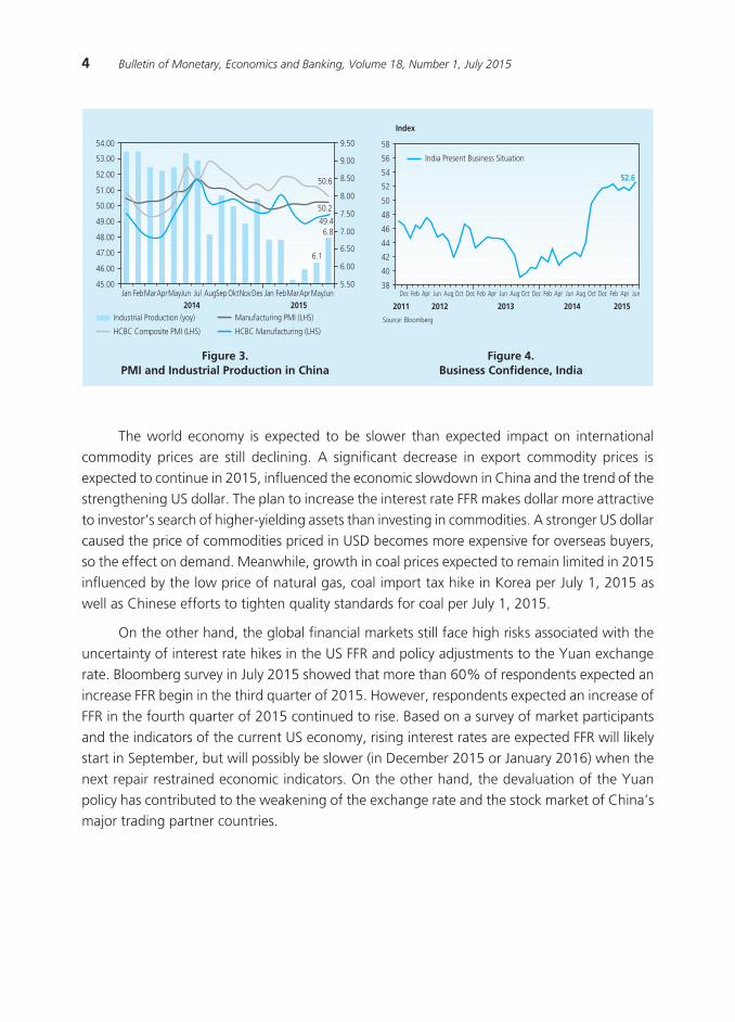
China’s economy is still slowing. This condition is reflected in the total PMI (HSBC Composite PMI) which are in a downward trend, although still in the expansion zone (Figure 3). In terms of investment, Fixed Asset Investment (FAI) is still weak, although it has begun to rebound. Industrial profits grew back negative.
Meanwhile, the Chinese stock market fell deep enough, mainly driven by worries that China’s stock valuation is too high. To stimulate the economy and weakening hold shares, Bank of China (PBoC) lowered the interest rates on loans and deposits on July 13, 2015 to a level of 4.85% and 2%. The impact of monetary policy is already visible, including the increasing growth of aggregate financing and new Yuan loans.
The Japanese economy is expected to be lower than initially estimated. Domestic demand weakened, reflected in growth of retail sales and department stores. Weakening domestic demand also boosted by real wage growth is still negative. Real wages also recorded negative results in consumer confidence have not improved. Production activity is still weak, as reflected in the index of production are still negative.
The Indian economy is still growing in line with initial estimates. India’s economic growth backed by improved consumption and investment. Improvement reflected in higher consumption growth in car sales. Meanwhile, India’s total direct investment from January to April 2015 reached 20.1 billion US dollars, an increase of 37.2% over the same period the previous year. With these developments, the level of business confidence also increased in line with the government policy of structural reforms that continue to run (Figure 4).
���
���
���
���
���
���
����
������ �� �� �� �� ��
���� ����
���� � � ������������������������ ��������������� ���
����
���
���������
����
���
���������
����
���
������
���
����
���
���������
����
���
���������
����
���
���������
�������������������
������ ��� ��� ������ ��� ��� ������ ��� ��������� ��� ��� ������ ��� ��������� ��� ��� ������ ��� ������������� ���� ���� ���� ���� ���� ���� ����
��
��
��
��
��
�
�
�
�
�
�
������
������������������ ���������� �������������
�������������
�����������������
4 Bulletin of Monetary, Economics and Banking, Volume 18, Number 1, July 2015
The world economy is expected to be slower than expected impact on international commodity prices are still declining. A significant decrease in export commodity prices is expected to continue in 2015, influenced the economic slowdown in China and the trend of the strengthening US dollar. The plan to increase the interest rate FFR makes dollar more attractive to investor’s search of higher-yielding assets than investing in commodities. A stronger US dollar caused the price of commodities priced in USD becomes more expensive for overseas buyers, so the effect on demand. Meanwhile, growth in coal prices expected to remain limited in 2015 influenced by the low price of natural gas, coal import tax hike in Korea per July 1, 2015 as well as Chinese efforts to tighten quality standards for coal per July 1, 2015.
On the other hand, the global financial markets still face high risks associated with the uncertainty of interest rate hikes in the US FFR and policy adjustments to the Yuan exchange rate. Bloomberg survey in July 2015 showed that more than 60% of respondents expected an increase FFR begin in the third quarter of 2015. However, respondents expected an increase of FFR in the fourth quarter of 2015 continued to rise. Based on a survey of market participants and the indicators of the current US economy, rising interest rates are expected FFR will likely start in September, but will possibly be slower (in December 2015 or January 2016) when the next repair restrained economic indicators. On the other hand, the devaluation of the Yuan policy has contributed to the weakening of the exchange rate and the stock market of China’s major trading partner countries.
Figure 3. PMI and Industrial Production in China
Figure 4. business Confidence, India
�����
�����
�����
�����
�����
�����
�����
�����
�����
�����
����
����
����
����
����
����
����
����
������� ��������������� ��� ��������������� ��� ���������������
���� �������������������������������
������������������������
�����������������������
������������������������
����
����
�������
���
��� ��� ��� ��� ��� ��� ��� ��� ��� ��� ��� ��� ��� ��� ��� ��� ��� ��� ��� ��� ��� �����
��
��
��
��
��
��
��
��
��
��
���� ���� ���� ���� ����
�����������������
�����
��������������������������������
����
5Quarterly Outlook on Monetary, Banking, and Payment System In Indonesia: Quarter II, 2015
II. THE DYNaMIC oF INDoNESIaN MaCRoECoNoMIC
2.1. Economic Growth
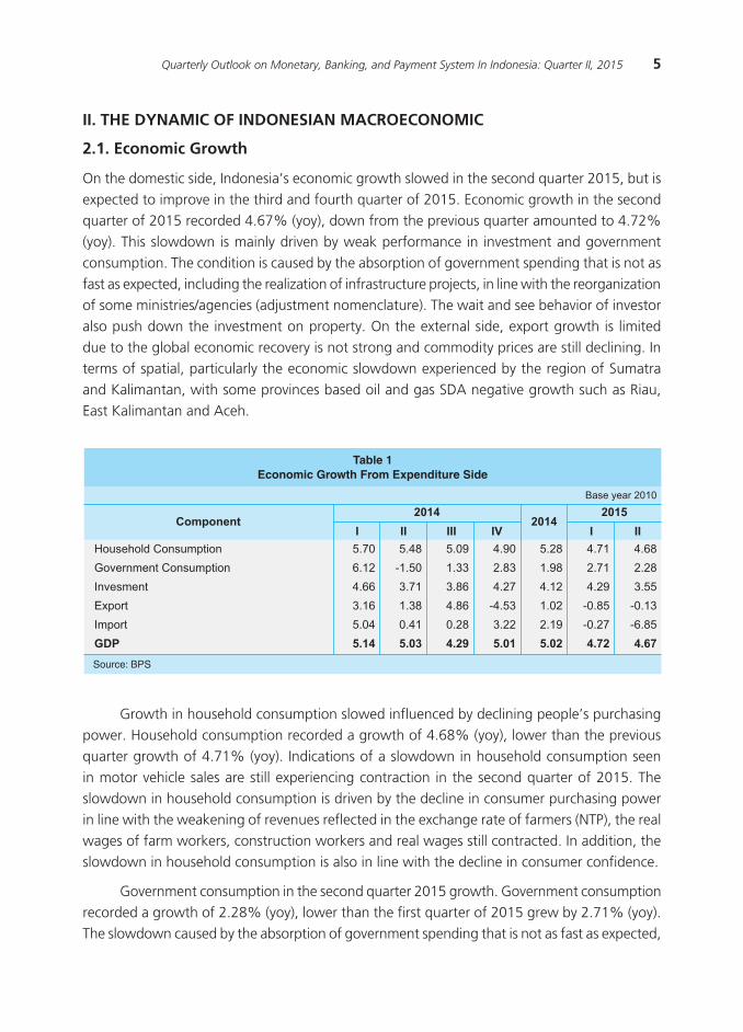
On the domestic side, Indonesia’s economic growth slowed in the second quarter 2015, but is expected to improve in the third and fourth quarter of 2015. Economic growth in the second quarter of 2015 recorded 4.67% (yoy), down from the previous quarter amounted to 4.72% (yoy). This slowdown is mainly driven by weak performance in investment and government consumption. The condition is caused by the absorption of government spending that is not as fast as expected, including the realization of infrastructure projects, in line with the reorganization of some ministries/agencies (adjustment nomenclature). The wait and see behavior of investor also push down the investment on property. On the external side, export growth is limited due to the global economic recovery is not strong and commodity prices are still declining. In terms of spatial, particularly the economic slowdown experienced by the region of Sumatra and Kalimantan, with some provinces based oil and gas SDA negative growth such as Riau, East Kalimantan and Aceh.
��������������������������������������������
�����������
���� ����
���������������������
����������������������
���������
������
������
���
� �� ��� �� � ���������������
����
����
����
����
����
����
����
�����
����
����
����
����
����
����
����
����
����
����
����
����
����
�����
����
����
����
����
����
����
����
����
����
����
����
�����
�����
����
����
����
����
�����
�����
����
��������������
Growth in household consumption slowed influenced by declining people’s purchasing power. Household consumption recorded a growth of 4.68% (yoy), lower than the previous quarter growth of 4.71% (yoy). Indications of a slowdown in household consumption seen in motor vehicle sales are still experiencing contraction in the second quarter of 2015. The slowdown in household consumption is driven by the decline in consumer purchasing power in line with the weakening of revenues reflected in the exchange rate of farmers (NTP), the real wages of farm workers, construction workers and real wages still contracted. In addition, the slowdown in household consumption is also in line with the decline in consumer confidence.
Government consumption in the second quarter 2015 growth. Government consumption recorded a growth of 2.28% (yoy), lower than the first quarter of 2015 grew by 2.71% (yoy). The slowdown caused by the absorption of government spending that is not as fast as expected,
6 Bulletin of Monetary, Economics and Banking, Volume 18, Number 1, July 2015
spending items, in line with the reorganization of some ministries / agencies (adjustment nomenclature).
Investment growth also slowed in the second quarter was recorded in 2015, mainly driven by a slowdown in the investment performance of the building sector. Investment growth slowed from 4.29% (yoy) in the first quarter of 2015 to 3.55% (yoy) in the second quarter of 2015. Growth in construction investment is affected by the achievement of lower realization of the government’s infrastructure is still low. The wait and see behavior of the private investors also push down the property investment. Meanwhile, non-construction investment growth is still limited, as reflected in weak investment in machinery and contracted sales of heavy equipment. Limited non-construction investment performance was driven by exports and domestic demand remains weak. In addition, the limited improvement of non-construction investment is also in line with the decline in business sentiment and investment loans.
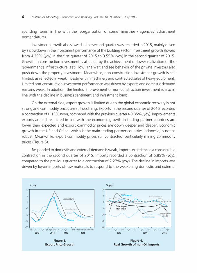
On the external side, export growth is limited due to the global economic recovery is not strong and commodity prices are still declining. Exports in the second quarter of 2015 recorded a contraction of 0.13% (yoy), compared with the previous quarter (-0,85%, yoy). Improvements exports are still restricted in line with the economic growth in trading partner countries are lower than expected and export commodity prices are down deeper and deeper. Economic growth in the US and China, which is the main trading partner countries Indonesia, is not as robust. Meanwhile, export commodity prices still contracted, particularly mining commodity prices (Figure 5).
Responded to domestic and external demand is weak, imports experienced a considerable contraction in the second quarter of 2015. Imports recorded a contraction of 6.85% (yoy), compared to the previous quarter to a contraction of 2.27% (yoy). The decline in imports was driven by lower imports of raw materials to respond to the weakening domestic and external
Figure 5. Export Price Growth
Figure 6. Real Growth of non-oil Imports
��
�
�
��
���
���
����� �� �� �� �� �� �� �� �� �� ��� ��� ��� ��� ��� ���
���� ���� ���� ����
�����������
�����������
�����
������
������
�� �� �� �� �� �� �� �� �� �����
���
���
���
�
��
��
���� ���� ����
������
���������� ��������������
���������������������
������������������������
�����

7Quarterly Outlook on Monetary, Banking, and Payment System In Indonesia: Quarter II, 2015
demand (Figure 6). Meanwhile, infrastructure spending is limited to make imports of capital goods contracted. Lower imports of capital goods were also driven by a contraction in the mining sector due to falling external demand.
By sector (activities), the economic slowdown in the second quarter of 2015 occurred in most sectors. This is also in line with demand conditions; the performance of most sectors of both tradable and non-tradable growth. Tradable sector slowdown came mainly from the contraction in mining and processing industry subsectors (ex. textiles, transport equipment and paper). The mining sector contracted quite in line with the decline in oil and gas lifting and coal production. In the manufacturing sector, although some sub-sectors slowed, the overall industrial sector grew quite well supported by the food and beverage industry. Meanwhile, the agricultural sector grew better supported by improved production of food related (Plant Foodstuff, Tabama) shift in the harvest season. On the other hand, most of the non-tradable sector grew slowly. A slowdown in the construction sector is still limited due to the realization of government projects and the wait-and-see behavior of the private actors. The trade sector also slowed in line with the still weak domestic consumption and imports were down very deep. In addition, utilities and other supporting sectors such as electricity supply, water supply and communication slowed in line with the slowdown in economic activity.
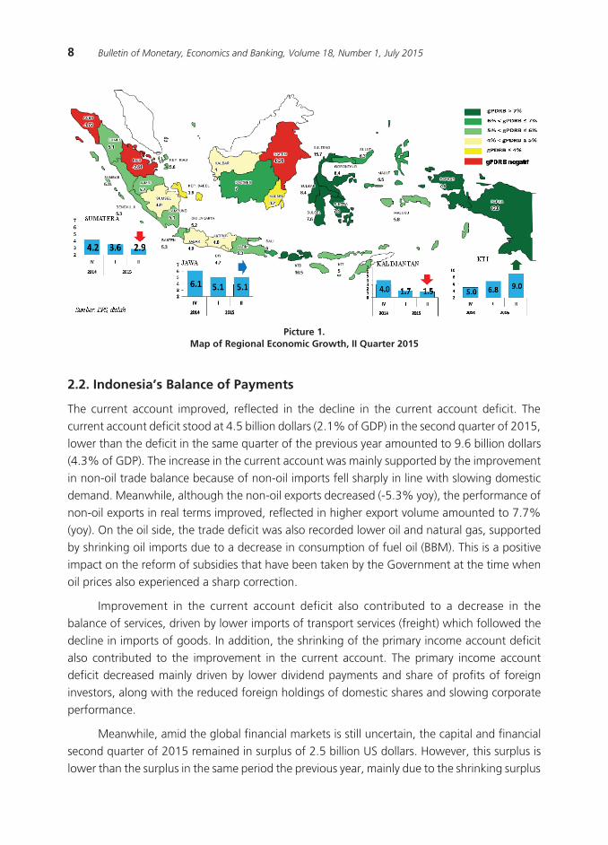
Spatially, the economic slowdown is mainly experienced by Sumatra and Kalimantan, with some provinces based natural resource (oil and gas) that the negative growth such as Riau, East Kalimantan and Aceh (Picture 1). In aggregate, the economic growth in Sumatra lowers growth than in previous quarters. The slowdown affected the limited increase in performance-related exports are still lower commodity prices that result in lower household consumption. Moreover, the continuing contraction of growth in Aceh and Riau due to lower oil and gas production has impacted on the economy Sumatra. Economic growth in Kalimantan also slowed compared with the previous quarter. The development was mainly influenced by the performance of coal exports are still limited due to the low prices in the global markets and weakening Chinese demand, as well as the limited absorption of local fiscal expenditure. Oil production still tends to fall even lead to economic growth in East Kalimantan back contraction. Economic developments in almost all regions in Java in the aggregate also grew slightly slowed. Java economic slowdown came mainly from the limited performance of manufacturing exports and investment. Meanwhile, the economy of various regions in eastern Indonesia (KTI) overall improved influenced by the base effect of mineral exports.2
2 Mineral exports can be done on a limited basis in the third quarter 2015 after the implementation of the ban on mineral export policy which took effect in January 2014.
8 Bulletin of Monetary, Economics and Banking, Volume 18, Number 1, July 2015
2.2. Indonesia’s balance of Payments
The current account improved, reflected in the decline in the current account deficit. The current account deficit stood at 4.5 billion dollars (2.1% of GDP) in the second quarter of 2015, lower than the deficit in the same quarter of the previous year amounted to 9.6 billion dollars (4.3% of GDP). The increase in the current account was mainly supported by the improvement in non-oil trade balance because of non-oil imports fell sharply in line with slowing domestic demand. Meanwhile, although the non-oil exports decreased (-5.3% yoy), the performance of non-oil exports in real terms improved, reflected in higher export volume amounted to 7.7% (yoy). On the oil side, the trade deficit was also recorded lower oil and natural gas, supported by shrinking oil imports due to a decrease in consumption of fuel oil (BBM). This is a positive impact on the reform of subsidies that have been taken by the Government at the time when oil prices also experienced a sharp correction.
Improvement in the current account deficit also contributed to a decrease in the balance of services, driven by lower imports of transport services (freight) which followed the decline in imports of goods. In addition, the shrinking of the primary income account deficit also contributed to the improvement in the current account. The primary income account deficit decreased mainly driven by lower dividend payments and share of profits of foreign investors, along with the reduced foreign holdings of domestic shares and slowing corporate performance.
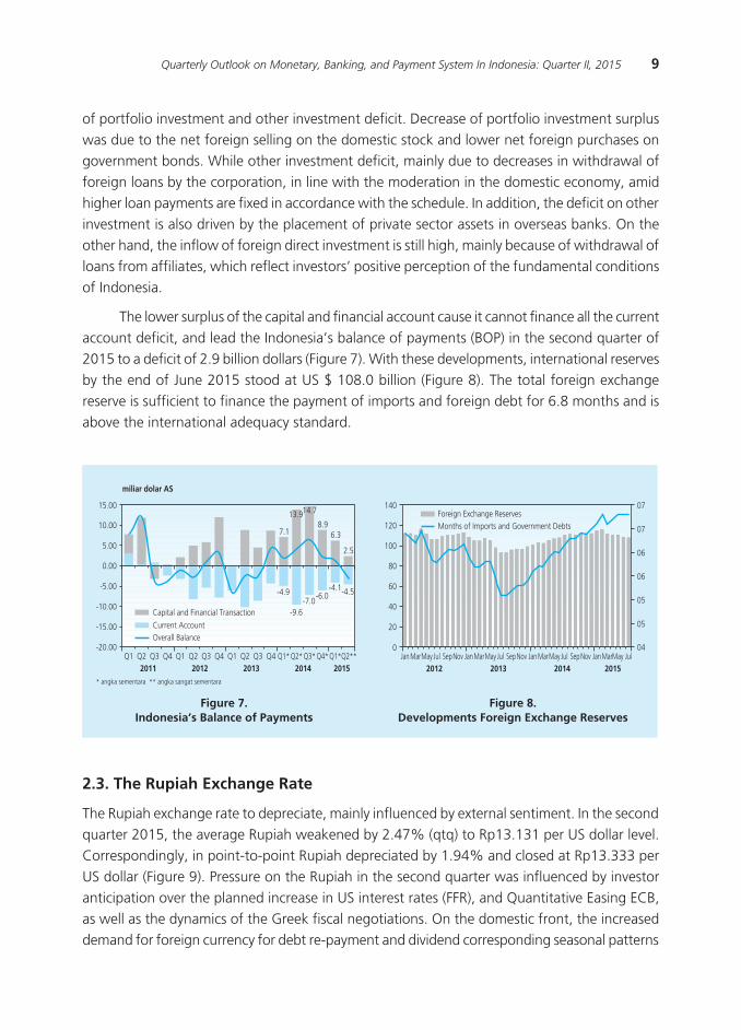
Meanwhile, amid the global financial markets is still uncertain, the capital and financial second quarter of 2015 remained in surplus of 2.5 billion US dollars. However, this surplus is lower than the surplus in the same period the previous year, mainly due to the shrinking surplus
Picture 1. Map of Regional Economic Growth, II Quarter 2015
9Quarterly Outlook on Monetary, Banking, and Payment System In Indonesia: Quarter II, 2015
of portfolio investment and other investment deficit. Decrease of portfolio investment surplus was due to the net foreign selling on the domestic stock and lower net foreign purchases on government bonds. While other investment deficit, mainly due to decreases in withdrawal of foreign loans by the corporation, in line with the moderation in the domestic economy, amid higher loan payments are fixed in accordance with the schedule. In addition, the deficit on other investment is also driven by the placement of private sector assets in overseas banks. On the other hand, the inflow of foreign direct investment is still high, mainly because of withdrawal of loans from affiliates, which reflect investors’ positive perception of the fundamental conditions of Indonesia.
The lower surplus of the capital and financial account cause it cannot finance all the current account deficit, and lead the Indonesia’s balance of payments (BOP) in the second quarter of 2015 to a deficit of 2.9 billion dollars (Figure 7). With these developments, international reserves by the end of June 2015 stood at US $ 108.0 billion (Figure 8). The total foreign exchange reserve is sufficient to finance the payment of imports and foreign debt for 6.8 months and is above the international adequacy standard.
2.3. The Rupiah Exchange Rate
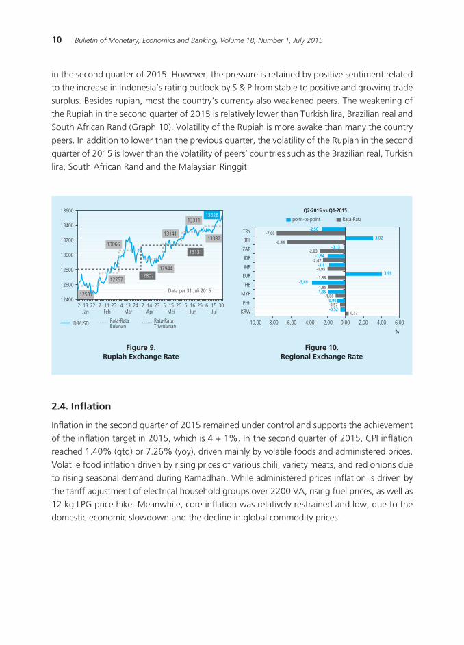
The Rupiah exchange rate to depreciate, mainly influenced by external sentiment. In the second quarter 2015, the average Rupiah weakened by 2.47% (qtq) to Rp13.131 per US dollar level. Correspondingly, in point-to-point Rupiah depreciated by 1.94% and closed at Rp13.333 per US dollar (Figure 9). Pressure on the Rupiah in the second quarter was influenced by investor anticipation over the planned increase in US interest rates (FFR), and Quantitative Easing ECB, as well as the dynamics of the Greek fiscal negotiations. On the domestic front, the increased demand for foreign currency for debt re-payment and dividend corresponding seasonal patterns
Figure 7.Indonesia’s Balance of Payments
Figure 8.Developments Foreign Exchange Reserves
�����
�����
����
����
�����
������
������
�������� �� �� �� �� �� �� �� �� �� �� �� �������������������
���� ���� ���� ���� ����
���������������
���������������������������������������������������������������
��������������������������������������������
����
������������
��������
���
������
��������
���
���
���
���
��
��
��
��
�
��
��
��
��
��
��
����������� ��� ������ ��������� ��� ������ ��������� ��� ������ ��������� ���
���� ���� ���� ����
���������������������������������������������������������������
10 Bulletin of Monetary, Economics and Banking, Volume 18, Number 1, July 2015
in the second quarter of 2015. However, the pressure is retained by positive sentiment related to the increase in Indonesia’s rating outlook by S & P from stable to positive and growing trade surplus. Besides rupiah, most the country’s currency also weakened peers. The weakening of the Rupiah in the second quarter of 2015 is relatively lower than Turkish lira, Brazilian real and South African Rand (Graph 10). Volatility of the Rupiah is more awake than many the country peers. In addition to lower than the previous quarter, the volatility of the Rupiah in the second quarter of 2015 is lower than the volatility of peers’ countries such as the Brazilian real, Turkish lira, South African Rand and the Malaysian Ringgit.
2.4. Inflation
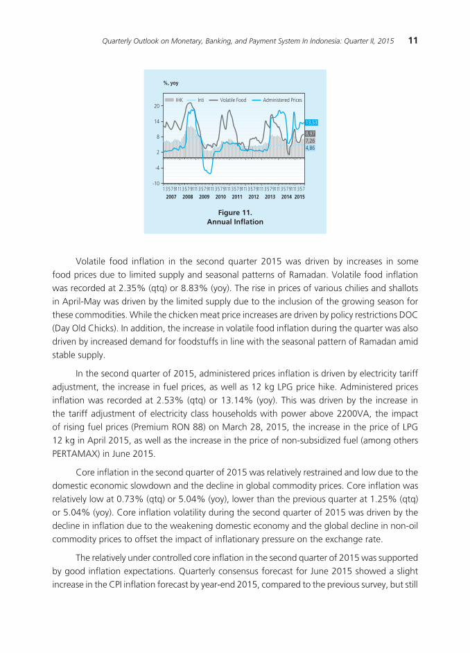
Inflation in the second quarter of 2015 remained under control and supports the achievement of the inflation target in 2015, which is 4 + 1%. In the second quarter of 2015, CPI inflation reached 1.40% (qtq) or 7.26% (yoy), driven mainly by volatile foods and administered prices. Volatile food inflation driven by rising prices of various chili, variety meats, and red onions due to rising seasonal demand during Ramadhan. While administered prices inflation is driven by the tariff adjustment of electrical household groups over 2200 VA, rising fuel prices, as well as 12 kg LPG price hike. Meanwhile, core inflation was relatively restrained and low, due to the domestic economic slowdown and the decline in global commodity prices.
Figure 9.Rupiah Exchange Rate
Figure 10.Regional Exchange Rate
� �� �� � �� �� � �� �� � �� �� � �� �� � �� �� � �� ����� ��� ��� ��� ��� ��� ���
�����
�����
�����
�����
�����
�����
�����
�����
�����
�����
�����
�����
�����
�����
�����
�����
�����
����������������
��������������������������
���������������������
���
���
���
���
���
���
���
���
���
���
�����
�����
�����
�����
�����
�����
�����
�����
����
����
����
�����
�����
�����
�����
�����
�����
�����
�����
�����
������ ����� ����� ����� ����� ���� ���� ���� ����
�
�����������������������
������������������
11Quarterly Outlook on Monetary, Banking, and Payment System In Indonesia: Quarter II, 2015
Volatile food inflation in the second quarter 2015 was driven by increases in some food prices due to limited supply and seasonal patterns of Ramadan. Volatile food inflation was recorded at 2.35% (qtq) or 8.83% (yoy). The rise in prices of various chilies and shallots in April-May was driven by the limited supply due to the inclusion of the growing season for these commodities. While the chicken meat price increases are driven by policy restrictions DOC (Day Old Chicks). In addition, the increase in volatile food inflation during the quarter was also driven by increased demand for foodstuffs in line with the seasonal pattern of Ramadan amid stable supply.
In the second quarter of 2015, administered prices inflation is driven by electricity tariff adjustment, the increase in fuel prices, as well as 12 kg LPG price hike. Administered prices inflation was recorded at 2.53% (qtq) or 13.14% (yoy). This was driven by the increase in the tariff adjustment of electricity class households with power above 2200VA, the impact of rising fuel prices (Premium RON 88) on March 28, 2015, the increase in the price of LPG 12 kg in April 2015, as well as the increase in the price of non-subsidized fuel (among others PERTAMAX) in June 2015.
Core inflation in the second quarter of 2015 was relatively restrained and low due to the domestic economic slowdown and the decline in global commodity prices. Core inflation was relatively low at 0.73% (qtq) or 5.04% (yoy), lower than the previous quarter at 1.25% (qtq) or 5.04% (yoy). Core inflation volatility during the second quarter of 2015 was driven by the decline in inflation due to the weakening domestic economy and the global decline in non-oil commodity prices to offset the impact of inflationary pressure on the exchange rate.
The relatively under controlled core inflation in the second quarter of 2015 was supported by good inflation expectations. Quarterly consensus forecast for June 2015 showed a slight increase in the CPI inflation forecast by year-end 2015, compared to the previous survey, but still
Figure 11.annual Inflation
��
��
�
�
��
���
������
���������������������������������������
� ������� ������� ������� ������� ������� ������� ������� ������� ������� ���� ���� ���� ���� ���� ���� ���� ����
�����
������������

12 Bulletin of Monetary, Economics and Banking, Volume 18, Number 1, July 2015
remained within the inflation target range. While the results of the Consumer Survey (SK) and the Retail Sales Survey (SPE) 3 months to come showed a decrease in expectations as seasonal factors passage of Ramadan and Eid.
Spatially, CPI inflation in the second quarter of 2015 is still quite high, especially in Sumatra and eastern Indonesia (KTI) (Picture 2). Sumatra region recorded the highest annual inflation rate compared to other areas, mainly due to high inflation in Bengkulu, Riau Islands, West Sumatra and Lampung. Meanwhile, highest inflation at region KTI in Maluku. Generally, the inflationary pressure in the second quarter of 2015 came from rising food commodity prices driven by increased demand with the arrival of Ramadan.
Picture 2.Regional Map of Inflation, Quarter 2015 (%, yoy)
III. THE DEVELoPMENTS IN MoNETaRY, baNKING aND PaYMENT SYSTEM
3.1. Monetary
The liquidity in interbank money market (Pasar Uang Antar Bank, PUAB) is maintained. The average overnight PUAB rate O/N in the second quarter 2015 declined from 5.84% to 5.66% (Figure 12). PUAB rates O/N DF down close Rate influenced by pressure decreased liquidity needs. Average position DF rate in the second quarter down from Rp138,68 trillion to Rp116,21 trillion. The average interest rate spread max-min in the interbank money market rose compared to the previous quarter from 88 bps to 101 bps (Figure 13). Nominally, the average volume of total PUAB in the second quarter of 2015 rise from Rp11,67 trillion to Rp13,03 trillion. The increase in the volume of PUAB total is contributed by the increase in the PUAB O / N which rise from Rp6,78 trillion to Rp7,08 trillion.
Inflation National: 7,26% (yoy)

13Quarterly Outlook on Monetary, Banking, and Payment System In Indonesia: Quarter II, 2015
The decline in deposit rates continues, while loan interest rates remained on hold. Weighted average in deposit rates (RRT) in the second quarter 2015 continued the downward trend from the previous quarter. Credit growth is still stuck and was lower than growth in deposits creating increased liquidity, so the deposit rates continue to decline. RRT deposit interest rate fell from 8.62% to 8.16% is contributed by the decline in short-term deposit rates (1 & 3 months) and category BUKU 43. Meanwhile, RRT lending rates in the second quarter 2015 was recorded at the level of 12, 97%, a slight decrease compared to the previous quarter, amounting to 12.99%. Retention decline in lending rates driven by increased credit risk factors. The decline in RRT lending rates mainly contributed by lower interest rates for working capital (KMK) and investment loans, each amounting to -12 and -3 bps. Meanwhile, RRT consumer loan interest rate rise by 14 bps. With these developments, the spread between interest rates on loans and deposits in the second quarter 2015 increased to 481 bps from 437 bps.
���
���
���
���
��
��
��
��
��
���
���
���
���
���
���
���
���
� ����
��� ��� ��� �� ��� ��� ��� ��� ��� ������� ���� ����
����������������
��������
������������������
���������
��������������������
����������������������������
����������������
�
�
�
�
�
�
�
�
�
�
�
�
���� ��� ��� ��� ��� ��� ��� ��� ���
���� ���� ����
���������
�������
�������
�������
Economic liquidity (M2) in the second quarter 2015 recorded slower growth driven by slower growth in quasi money and M1. M2 growth in the second quarter of 2015 decreased to 13.00% (yoy) of 16.26% (yoy) in the previous quarter. By component, M2 decrease comes from decreasing quasi-money, from 17.60% in the first quarter of 2015 to 13.90% in second quarter 2015 and a decrease in the growth of M1, from 12.19% (yoy) in the first quarter of 2015 to 9, 90% (yoy) in the second quarter of 2015. The decline in M1 growth was driven by a decrease in demand deposits Rupiah from 20.90% (yoy) in the first quarter of 2015 to 11.65% (yoy) in the second quarter of 2015. Meanwhile, the other components of M1, the fiat money, increased from 1.20% (yoy) in the first quarter of 2015 to 7.40% (yoy) in the second quarter, 2015.
3 Bank with core capital more than Rp30 trillion.
Figure 12.Monetary operations of Interest Rate Corridor
Figure 13. bI Rate, DF Rate and PUab oN Interest Rate
14 Bulletin of Monetary, Economics and Banking, Volume 18, Number 1, July 2015
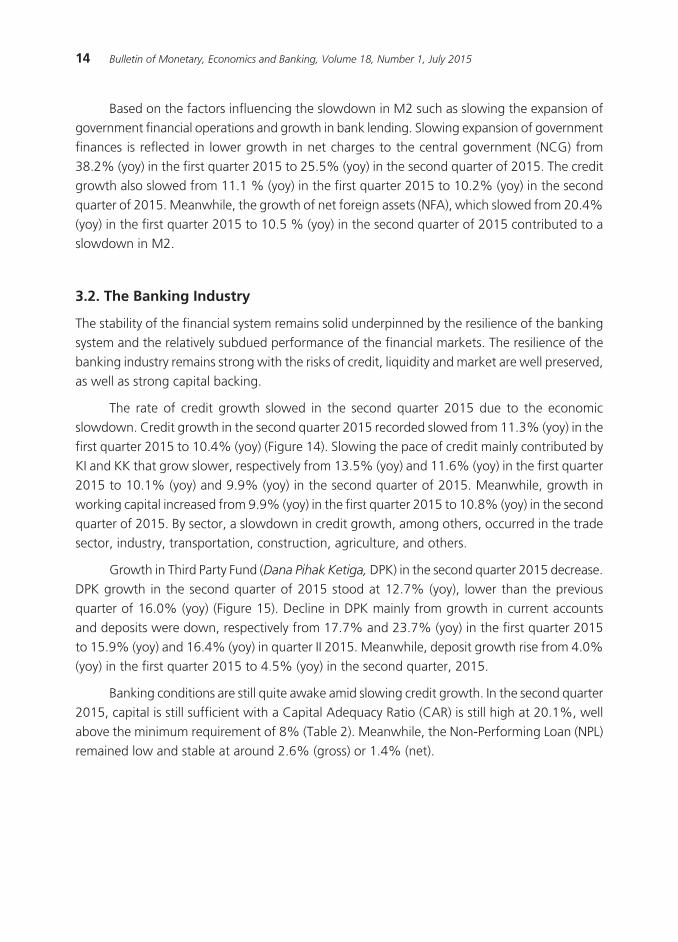
Based on the factors influencing the slowdown in M2 such as slowing the expansion of government financial operations and growth in bank lending. Slowing expansion of government finances is reflected in lower growth in net charges to the central government (NCG) from 38.2% (yoy) in the first quarter 2015 to 25.5% (yoy) in the second quarter of 2015. The credit growth also slowed from 11.1 % (yoy) in the first quarter 2015 to 10.2% (yoy) in the second quarter of 2015. Meanwhile, the growth of net foreign assets (NFA), which slowed from 20.4% (yoy) in the first quarter 2015 to 10.5 % (yoy) in the second quarter of 2015 contributed to a slowdown in M2.
3.2. The Banking Industry
The stability of the financial system remains solid underpinned by the resilience of the banking system and the relatively subdued performance of the financial markets. The resilience of the banking industry remains strong with the risks of credit, liquidity and market are well preserved, as well as strong capital backing.
The rate of credit growth slowed in the second quarter 2015 due to the economic slowdown. Credit growth in the second quarter 2015 recorded slowed from 11.3% (yoy) in the first quarter 2015 to 10.4% (yoy) (Figure 14). Slowing the pace of credit mainly contributed by KI and KK that grow slower, respectively from 13.5% (yoy) and 11.6% (yoy) in the first quarter 2015 to 10.1% (yoy) and 9.9% (yoy) in the second quarter of 2015. Meanwhile, growth in working capital increased from 9.9% (yoy) in the first quarter 2015 to 10.8% (yoy) in the second quarter of 2015. By sector, a slowdown in credit growth, among others, occurred in the trade sector, industry, transportation, construction, agriculture, and others.
Growth in Third Party Fund (Dana Pihak Ketiga, DPK) in the second quarter 2015 decrease. DPK growth in the second quarter of 2015 stood at 12.7% (yoy), lower than the previous quarter of 16.0% (yoy) (Figure 15). Decline in DPK mainly from growth in current accounts and deposits were down, respectively from 17.7% and 23.7% (yoy) in the first quarter 2015 to 15.9% (yoy) and 16.4% (yoy) in quarter II 2015. Meanwhile, deposit growth rise from 4.0% (yoy) in the first quarter 2015 to 4.5% (yoy) in the second quarter, 2015.
Banking conditions are still quite awake amid slowing credit growth. In the second quarter 2015, capital is still sufficient with a Capital Adequacy Ratio (CAR) is still high at 20.1%, well above the minimum requirement of 8% (Table 2). Meanwhile, the Non-Performing Loan (NPL) remained low and stable at around 2.6% (gross) or 1.4% (net).
15Quarterly Outlook on Monetary, Banking, and Payment System In Indonesia: Quarter II, 2015
������������������������������������
�������������
������������������
���� ����
��� ��� ��� ��� ��� ��� ��� ��� ��� ��� ��� ��� ��������������
���
�������
����
������������
���
���
���
������
������
������
���
���
���
���
���
�������
�������
�������
�����
����
�����
���
���
�������
�������
�������
�����
����
�����
���
���
�������
�������
�������
�����
����
�����
���
���
�������
�������
�������
�����
����
�����
���
���
�������
�������
�������
�����
����
�����
���
���
�������
�������
�������
�����
����
�����
���
���
�������
�������
�������
�����
����
�����
���
���
�������
�������
�������
�����
����
�����
���
���
�������
�������
�������
�����
����
�����
���
���
�������
�������
�������
�����
����
�����
���
���
�������
�������
�������
�����
����
�����
���
���
�������
�������
�������
�����
����
�����
���
���
�������
�������
�������
�����
����
�����
���
���
3.3. The Stock Market and Government Securities Market
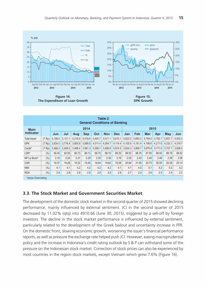
The development of the domestic stock market in the second quarter of 2015 showed declining performance, mainly influenced by external sentiment. JCI in the second quarter of 2015 decreased by 11.02% (qtq) into 4910.66 (June 30, 2015), triggered by a sell-off by foreign investors. The decline in the stock market performance is influenced by external sentiment, particularly related to the development of the Greek bailout and uncertainty increase in FFR. On the domestic front, slowing economic growth, worsening the issuer’s financial performance reports, as well as pressure the exchange rate helped push JCI. However, easing macroprudential policy and the increase in Indonesia’s credit rating outlook by S & P can withstand some of the pressure on the Indonesian stock market. Correction of stock prices can also be experienced by most countries in the region stock markets, except Vietnam which grew 7.6% (Figure 16).
Figure 14. The Expenditure of Loan Growth
Figure 15. DPK Growth
��
��
��
��
��
��
��
�
�
������
��� ��� ��� ��� ��� ��� ��� ��� ��� ��� ��� ��� ��� ��� ��� ��� ��� ������� ���� ���� ����
�����
���
��
��
��������������
���
���
���
���
���
���
��
��
���
���
���
���
���
��
��
����������
�������
�����
���������
��� ��� ��� ������ ��� ��� ��� ��� ������ ��� ��� ��� ��� ������ ��� ��� ��� ������� ���� ���� ����
16 Bulletin of Monetary, Economics and Banking, Volume 18, Number 1, July 2015
SBN market performance in the second quarter 2015 decline, reflected in the rising yield on government securities for all tenors. In line with the stock market, the decline in the performance of the government securities market is also the impact of external sentiment. The weakening performance of government securities is affected by global sentiment still high investor concerns related to the development of Greek debt, FFR hike expectations, as well as expectations of slowing global economy after the release of manufacturing data from China. Overall yield on government securities rose by 81 bps from 7.42% to 8.22%. The yield on short, medium and long respectively increased by 80 bps, 87 bps and 69 bps to 7.84%, 8.31% and 8.54%. Meanwhile, the benchmark 10-year yield rose by 89 bps from 7.44% to 8.33% (Figure 17). On the other hand, the increase in yield of government securities continued to encourage foreign investors to buy government securities that foreign ownership in the second quarter of 2015 increased to 38.62% from 37.40% in the previous quarter. Despite decreased compared to the previous quarter, the second quarter non-resident investors recorded a net buy of Rp33,46 trillion.
3.4. Non-bank Financing
Nonbank financing of the economy in the second quarter of 2015 increased compared to the previous quarter. Total financing for the second quarter of 2015 through the issuance of IPO, rights issues, corporate bonds, medium term notes (MTN), promissory notes and other financial institutions reached Rp47,4 trillion or higher than the first quarter of 2015 amounted to only Rp22,2 trillion. In the composition, the biggest increase contributed by the increase in financing through the issuance of bonds that reached Rp26,1 trillion. However, financing through the issuance of shares as well as MTN and NCD (negotiable certificate of deposit) also increased compared to the previous quarter respectively amounting to Rp14.3 trillion and Rp7 trillion.
Figure 16. JCI and Global Stock Index, Quarter 2015 (qtq)
Figure 17. Yield Changes, Quarter 2015
���� ���� ��� �� �� ��� ��� ���
�����������������������
������������������������
�������������������������������������
��������������������������������������
������������������������������������������
��������������������
�����
������
����������
����������
����������
���������������
����
���������
����
�
���
�
���
�
���
�
� ���
���
��
��
��
��
��
��
��
��
��
�� � � � � � � � � �� �� �� ��
�����
������������������������� �������� ��������
17Quarterly Outlook on Monetary, Banking, and Payment System In Indonesia: Quarter II, 2015
3.5. The Development of Payment Systems
In general, the development of cash payment systems is in line with domestic economy, especially the household consumption. Average the distributed currencies (Uang Kartal yang
Diedarkan, UYD) in the second quarter 2015 amounted Rp506.6 trillion or grew by 9.0% (yoy), from the previous quarter amounted Rp462,6 trillion. Increased growth is in line with the increasing demand for cash, especially by household consumption sector entering the period of Holy Ramadhan, 2015.
In the middle of UYD growth trends that influenced the cyclical factors, Bank Indonesia continues to improve the quality of money in circulation. During the second quarter of 2015, some 1.2 billion non-usable pieces /chips (Uang Tidak Layak Edar, UTLE); worth Rp33.4 trillion had been destroyed and replaced for circulation. Total annihilation UTLE was lower compared to the first quarter of 2015 stood at 1.5 billion pieces / chips or Rp40,9 trillion. The reduced number of destroyed UTLE was caused partly by the decline in the inflow of Rupiah from banks to Bank Indonesia.
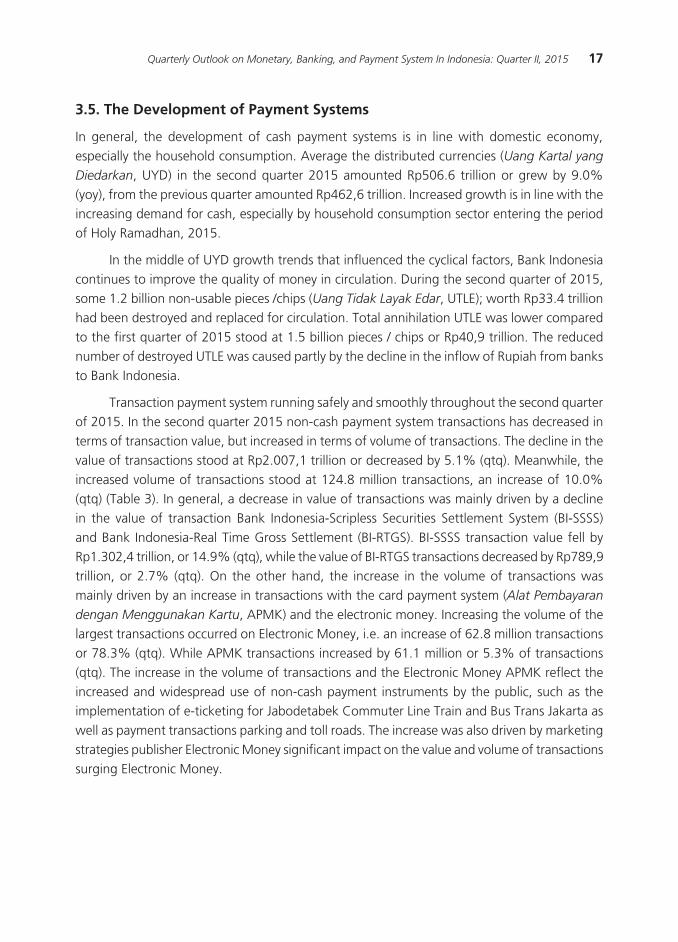
Transaction payment system running safely and smoothly throughout the second quarter of 2015. In the second quarter 2015 non-cash payment system transactions has decreased in terms of transaction value, but increased in terms of volume of transactions. The decline in the value of transactions stood at Rp2.007,1 trillion or decreased by 5.1% (qtq). Meanwhile, the increased volume of transactions stood at 124.8 million transactions, an increase of 10.0% (qtq) (Table 3). In general, a decrease in value of transactions was mainly driven by a decline in the value of transaction Bank Indonesia-Scripless Securities Settlement System (BI-SSSS) and Bank Indonesia-Real Time Gross Settlement (BI-RTGS). BI-SSSS transaction value fell by Rp1.302,4 trillion, or 14.9% (qtq), while the value of BI-RTGS transactions decreased by Rp789,9 trillion, or 2.7% (qtq). On the other hand, the increase in the volume of transactions was mainly driven by an increase in transactions with the card payment system (Alat Pembayaran
dengan Menggunakan Kartu, APMK) and the electronic money. Increasing the volume of the largest transactions occurred on Electronic Money, i.e. an increase of 62.8 million transactions or 78.3% (qtq). While APMK transactions increased by 61.1 million or 5.3% of transactions (qtq). The increase in the volume of transactions and the Electronic Money APMK reflect the increased and widespread use of non-cash payment instruments by the public, such as the implementation of e-ticketing for Jabodetabek Commuter Line Train and Bus Trans Jakarta as well as payment transactions parking and toll roads. The increase was also driven by marketing strategies publisher Electronic Money significant impact on the value and volume of transactions surging Electronic Money.

18 Bulletin of Monetary, Economics and Banking, Volume 18, Number 1, July 2015
IV. THE ECoNoMIC oUTLooK
Bank Indonesia forecasts the economy will improve in the second half of 2015. Economic growth in the third and fourth quarter 2015 are expected to be higher than the first and second quarter 2015 respectively by 4.72% (yoy) and 4.67% (yoy), Higher economic growth was supported by domestic demand, particularly investment, in line with the implementation of government infrastructure projects are getting stronger. Household consumption (including LNPRT) grows on an upward trend, supported by expectations of improved earnings and the simultaneous local elections in the fourth quarter of 2015. From the external, economic improvement is supported by the improved export performance in line with global economic recovery, although still in limited magnitude. With an increase in domestic demand and better export, then import is expected to grow stronger.
Inflation in 2015 is predicted to be lower than the previous year and remain within the inflation target range by 2015. On the domestic front, inflationary pressures from the demand side are forecasted relatively minimal, in line with the forecast slowdown in economic growth in 2015. Inflation expectations are also expected to be maintained with the support policies and good coordination between Bank Indonesia and the Government. Inflationary pressure from external factors is predicted not too large, in line with the forecasts of the limited increase in international commodity prices. Relatively moderate inflationary pressures originating from the above three factors are expected to offset rising inflation pressures coming from the increase in import duties on several consume goods, dried up because of the strengthening of the El Nino phenomenon, as well as an upward correction some food commodity prices. However, some risks that can interfere with the achievement of the inflation target range, such as the weakening of the Rupiah and the limited rice imports amid falling production due to El Nino, need to be wary.
��������������������������������������������������������������
����������������������������������
���� ���� ���������
���� ����� ���� ��� ���� �������������
�������
�������
���������
����
������
����
�����������
��������
����������������
�����
��������
�������
�����
�����
�����
�������
����
�������
���
��������
��������
�������
�����
�����
�����
�������
����
�������
���
��������
��������
��������
�����
�����
�����
�������
����
�������
���
��������
��������
�������
�����
�����
�����
�������
����
�������
���
��������
��������
�������
�����
�����
�����
�������
����
�������
���
��������
�����
������
����
�����
����
����
����
����
�����
�����
�������������������

19Quarterly Outlook on Monetary, Banking, and Payment System In Indonesia: Quarter II, 2015
Bank Indonesia will keep closely watching some economic risks originating from external and domestic. From the global side, the risk of exchange rate depreciation could destabilize the economy in the short term and the future economic outlook. Uncertainties related to global sentiment rise in the Fed Funds rate, the policy continued devaluation of the Yuan by the Chinese authorities and the Malaysian Ringgit risk weakening pressure on the exchange rate, inflation, and economic growth. Another source of global risk outlook for world economic growth and commodity prices in the international market. On the domestic front, the effectiveness of fiscal stimulus is the key improvement of short-term economic growth prospects. The impact of the El Nino phenomenon also needs attention because it affects the outlook for inflation and economic growth.

20 Bulletin of Monetary, Economics and Banking, Volume 18, Number 1, July 2015
This page intentionally left blank

21The Role of Macroprudential Policy to Control Exchange Rate Volatility, Liquidity, And Bank Credit
THE ROLE OF MACROPRUDENTIAL POLICY TO CONTROL EXCHANGE RATE VOLATILITY,
LIQUIDITY, AND BANK CREDIT
Muhammad Edhie Purnawan1
M. Abd. Nasir
This paper analyzes the macroprudential policy by the central bank to maintain the financial
system stability. Using panel data of the government banks, foreign, private, joint venture, and regional
development banks during 2004- 2012, we employ Vector Autoregressive Exogenous (VARX) and event
analysis method and find that the level of exchange rate volatility decrease after the implementation of
the one month holding period, six-month holding period and net open position policies. However, for
the nominal exchange rate, these policies are not effective. In aggregate the reserve requirement plus
loan to deposit ratio policy is effective to raise the bank credit allocation. Furthermore, the impact of the
primary reserve policy is very limited to lower the liquidity of the economy; while at the same time the
flow of foreign capital comes into very heavy.
Abstract
Keywords: macroprudential policy, VARX, event analysis, holding period, net open position, reserve
requirement, banking.
JEL Classification: E51, E58, E60, E69
1 Muhammad Edhie Purnawan (corresponding author: [email protected]) is Vice Dean at the Faculty of Economics and Business, Universitas Gadjah Mada ; M. Abd. Nasir (email: [email protected]) is Lecturer at the Department of Economics and Development Studies, Faculty of Economics, University of Jember.
22 Bulletin of Monetary, Economics and Banking, Volume 18, Number 1, July 2015
I. INTRODUCTION
The term of “macroprudential” was first used in the late 1970s in an unpublished document by Cooke Committee (founder of the Basel Committee on Banking Supervision) and the Bank of
England (Clemment, 2010: 2). There are several definitions of macroprudential policy. According to the version of the Working Group G-20 (2010: 4), macroprudential policy is a policy aimed at increasing the resilience of the financial system and to mitigate systemic risk arising from the linkages between institutions and financial institutions to follow the trend of the economic cycle (procyclical), thus increasing systemic risk.
The crisis in the United States in September 2008, which then spread to various countries of the world shows that the instability in the financial sector have a serious impact on the real sector (Agung, 2010: 2). The financial crisis fueled by credit bubbles turned into a global crisis and has led to a drastic drop in economic activities.
Claessens et al., (2012: 9) and Hahm et al., (2011: 15) argues that there are three important lessons from the financial crisis. The first is the impact of developments in the financial sector to the real sector was greater than original estimates. The second is the cost of saving a huge crisis. Third is price stability and output did not ensure financial stability. Therefore, formulate a policy framework to address the instability of the financial system that macroprudential policy.
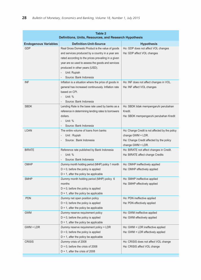
Based on the arguments Angelini et al., (2012: 20) and Tovar et al., (2012: 27) macroprudential instrument used to mitigate systemic risk in three categories, namely the risks caused by too strong credit growth, liquidity risk, and risks due to heavy capital inflows. Some macroprudential policy instruments that had been conducted by Bank Indonesia is Month Holding Period (MHP), Net Open Position (NOP), Reserve Requirement / Giro Wajib Minimum (GWM), and GWM + LDR (Credit to Deposit Ratio).
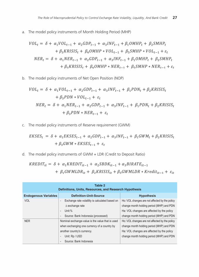
Month Holding Period (MHP) is a policy that requires buyers of Bank Indonesia Certificates (SBI) in both the primary and secondary markets hold its ownership of SBI during the specified time period is 1 month (OMHP) and 6 months (SMHP) from the date of purchase, before it can be traded to other parties. Month holding period (MHP) policy aims to reduce the volatility of the flow of funds in SBI and improve the effectiveness of monetary management. This policy is expected to minimize the negative impact of foreign capital flows for speculative or short-term to monetary and financial system stability and can encourage other transactions in the money market.2
Net Open Position (NOP) is the sum of the absolute values of the net difference between assets and liabilities in the balance sheet for each foreign exchange the net difference between
2 Explanation of the month holding period based on Bank Indonesia Regulation. Number: 12/11 / PBI / 2010 about the Monetary Operations.
23The Role of Macroprudential Policy to Control Exchange Rate Volatility, Liquidity, And Bank Credit
3 Based on Bank Indonesia Regulation Number: 5/13/PBI/2003 about the Net Open Position of Commercial Bank then refined into a Bank Indonesia Regulation 12/10/PBI/2010 about the Third Amendment to Bank Indonesia Regulation. No. 5/13/ PBI/2003.
4 Based on Bank Indonesia Regulation Number: 12/19/PBI/2010 about Reserve Requirement of Commercial Banks in Bank Indonesia in Rupiah and Foreign Exchange.
5 Based on Bank Indonesia Regulation No. 15/7/PBI/2013 on the Second Amendment to Bank Indonesia Regulation No. 12/19/ PBI/2010 about the Reserve Requirement of Commercial Banks in Bank Indonesia in Rupiah and Foreign Exchange.
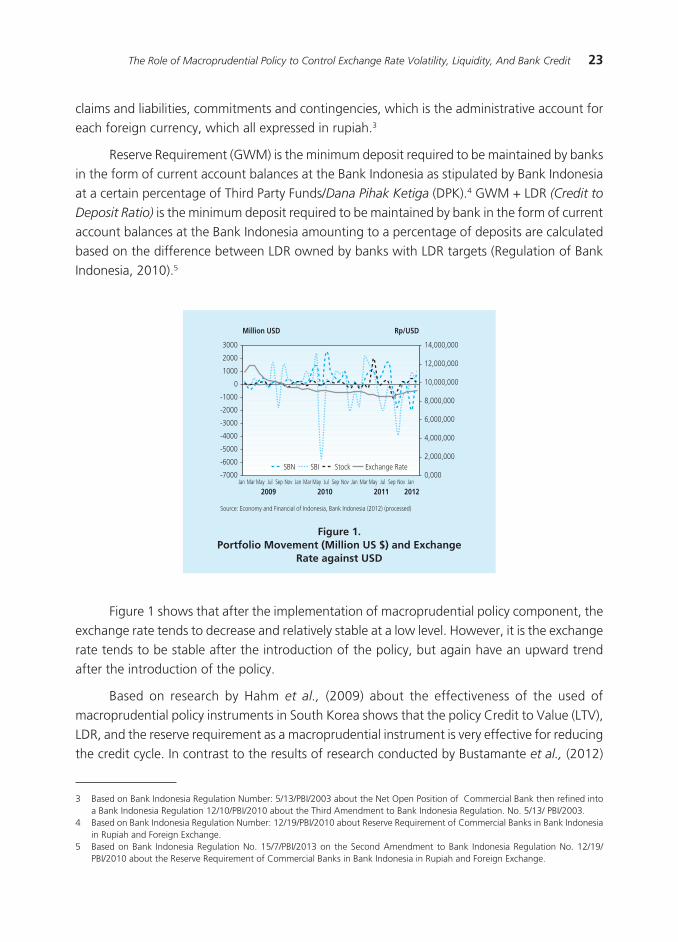
Figure 1.Portfolio Movement (Million US $) and Exchange
Rate against USD
claims and liabilities, commitments and contingencies, which is the administrative account for each foreign currency, which all expressed in rupiah.3
Reserve Requirement (GWM) is the minimum deposit required to be maintained by banks in the form of current account balances at the Bank Indonesia as stipulated by Bank Indonesia at a certain percentage of Third Party Funds/Dana Pihak Ketiga (DPK).4 GWM + LDR (Credit to
Deposit Ratio) is the minimum deposit required to be maintained by bank in the form of current account balances at the Bank Indonesia amounting to a percentage of deposits are calculated based on the difference between LDR owned by banks with LDR targets (Regulation of Bank Indonesia, 2010).5
Figure 1 shows that after the implementation of macroprudential policy component, the exchange rate tends to decrease and relatively stable at a low level. However, it is the exchange rate tends to be stable after the introduction of the policy, but again have an upward trend after the introduction of the policy.
Based on research by Hahm et al., (2009) about the effectiveness of the used of macroprudential policy instruments in South Korea shows that the policy Credit to Value (LTV), LDR, and the reserve requirement as a macroprudential instrument is very effective for reducing the credit cycle. In contrast to the results of research conducted by Bustamante et al., (2012)

24 Bulletin of Monetary, Economics and Banking, Volume 18, Number 1, July 2015
in which the effectiveness of the use of macroprudential instruments in Colombia shows that the LTV is less effective policy applied.
Other researchers that Tovar et al., (2012) in his study in Brazil, Colombia, and Peru show that the use of macroprudential instruments such as reserve requirement effectively applied in Brazil and Peru, while Colombia is not. Then Lim et al., (2011) evaluated the effectiveness of the use of macroprudential instruments in reducing systemic risk in 49 countries. They argue that most of the instruments (LTV and GWM) is effective in reducing procyclicality, but its effectiveness is highly dependent on the financial sector shocks.
Based on these descriptions, then this research will be limited by the following two research questions; first, how macroprudential policy instruments target movement before and after the policy is implemented?, second, how the effectiveness of macroprudential policy instruments (month holding period, net open position, reserve requirement, reserve requirement and credit to deposit ratio) which has been applied in Indonesia?
The next section of this paper presents the theoretical background and related empirical studies. Section three present the data and estimated model. Section four discuss the estimation result and its analysis, while section four present the conclusion and policy implications.
II. THEORY
Macroprudential policy is prudential regulatory instrument that is intended to encourage the stability of the financial system as a whole, not the individual health of financial institutions (the
International Monetary Fund, 2013: 12; Schloenmaker and Peter, 2011: 23). The purpose of monetary policy is to stabilize prices of goods and services in the economy. Meanwhile, the goal of macroprudential policy is to ensure the durability of the overall financial system in order to maintain the supply of financial intermediation services to the overall economy (Quint and Pau 2011: 11 and Milne, 2009: 19).
There are two important dimensions of macroprudential policy (Claessens et al., 2012: 98; Tovar et al., 2012: 29, and Lima et al., 2012: 19). First, the dimension of the cross section which shifts the focus of prudential regulation that is applicable to individual financial institutions towards the regulation of the overall system. The second dimension is the dimension of time-series, which macroprudential policies aimed at reducing the risk of excessive procyclicality in the financial system.
The purpose of the macroprudential policy is countercyclical which will work together with the goal of monetary policy in reducing economic fluctuations (Arnoldet al., 2012: 3127; Gersbach and Rochet, 2012: 83). Operationally, a number of studies have been carried out to design a macroprudential policy countercyclical (Bank of England 2011: 5; Arregui et al., 2012: 13; Buncic and Martin, 2013: 356). In the context of regulatory capital requirements, regulatory

25The Role of Macroprudential Policy to Control Exchange Rate Volatility, Liquidity, And Bank Credit
capital instruments that are countercyclical is capital or surcharge added above the minimum capital required by regulation mikroprudensial. Additional capital must be dynamic (time-varying
capital surcharge), varies countercyclical, rising when the economy is rising to put the brakes on the growth of bank balance and fell down when the period is to provide incentives for banks to continue to lend (Bank of England 2011: 8).
The use of macroprudential instruments is actually not a new thing, it’s just such instruments more widely applied after the global crisis in 2008. The use of the instrument depends on the level of economic and financial development, exchange rate regime, and durability (vulnerability) to shocks (Delgado and Mynor 2011: 28). These instruments are often used in complement with other macroeconomic policies, such as monetary policy and fiscal policy, and serves as an automatic stabilizer.
Basically macroprudential policy instruments can be grouped into three parts as shown in Table 1.
�����������������������������������������
�������� ������
������
���������
�������
�����������
��� �������������������������������������
��� ��������������������������������������
��� ��������������������������������
��� �����������������������������������
��� ����������������������������������������������
��������������
�������������������������������
������������������������
��� ���������������������������������������������������
���������������������������������������
���������������������������������������
��������������
��������������
��������������
��������������
���������������
���������������
��������������
��������������
��������������
��������������
����������������������������������������������������������������������
Implementation of these instruments is done by learning and applying it. Calibration trials performed depending on the type of shocks faced (Lima et al., 2012: 15). From the point of view of Galati and Richhild (2011: 27) and CGFS (2010: 16-18), the design and calibration of the instrument is usually based on discretion, not based on the rules. Macroprudential instruments are used with the level of discretion that is dominant compared to the basic rules given the high uncertainty in the run macroprudential policy. The advantage of this discretion is a high flexibility in answering instruments in accordance with the experience and information gained (Beauet al., 2012: 17). The model is only used for the simulation, while for the determination
26 Bulletin of Monetary, Economics and Banking, Volume 18, Number 1, July 2015
of the level of the instrument is done through discretionary (Tovar et al., 2012: 21). The effectiveness of this policy instrument is still considered tentative given application is usually done in conjunction with monetary policy.
In general, macroprudential policy instruments are applied in some countries differ from each other depending on the level of economic growth and stability of the financial system of the country. Research Hahm et al., (2009) in South Korea shows that the LTV policy, LDR, and the reserve requirement as a macroprudential instrument is very effective for reducing the credit cycle. In contrast, strict policies are not effective precisely to prevent credit bubbles. They also argue that the addition of the objectives of this policy will make the confusion about the central bank’s commitment to financial stability.
In line with research conducted by Tovar et al., (2012) in Brazil, Colombia, and Peru which shows that the use of macroprudential instruments such as reserve requirement effectively applied in Brazil and Peru, while Colombia is not effective. This is because the rate of credit growth in Colombia is relatively smaller than in Brazil and Peru as well as the gap between the high currencies exchange rate is to credits granted by banks in the country.
Another case study conducted by Bustamante et al. (2012), which examined the effectiveness of the use of macroprudential instruments such as LTV in Colombia. His research shows that the LTV is less effective policy applied due to rising house prices are used as collateral for credits so that, on average, can reduce the LTV ratio and will cut their lending rates.
Then, the research conducted by Lim et al. (2011) evaluated the effectiveness of the use of macroprudential instruments in reducing systemic risk in 49 countries. They argue that most of the instruments (LTV and GWM) is effective in reducing procyclicality, but its effectiveness is highly dependent on the turbulence in the financial sector.
III. METHODOLOGY
The data used in this study are secondary data from time series data and panel data. Period of the data used are monthly data from the period 2004M1-2012M12.While the cross section data is a type of bank in Indonesia, namely the state banks, foreign banks, joint venture banks, private banks, and regional development banks. The unit of analysis of this study is a commercial bank in Indonesia. The data used in this study were obtained from Statistik Ekonomi dan Moneter
Indonesia (SEMI), Statistik Perbankan Indonesia (SPI), dan Statistik Ekonomi dan Keuangan
Indonesia (SEKI), which is where all the data published by Bank Indonesia.
Specification of the model used in answering the research question will modify the model to research conducted by Tovar et al. (2012), Hahm et al. (2011) and Bustamante et
al. (2012).
27The Role of Macroprudential Policy to Control Exchange Rate Volatility, Liquidity, And Bank Credit
a. The model policy instruments of Month Holding Period (MHP)
c. The model policy instruments of Reserve requirement (GWM)
d. The model policy instruments of GWM + LDR (Credit to Deposit Ratio)
b. The model policy instruments of Net Open Position (NOP)
�������������������������������������������������������������
�������������������� ����������
���
���
���
���
����
����
������
����
����
����
���
���������
������
����������������������
� �����������������������������������������������
����������������
� ������
� ����������������������������������
������������������������������������������������
��������������������������������������������
���������������������������
� ��������������
� ����������������������
�������������������������������������������������
������������������������������������������������
���������������������������������������������������
�������������������������������������������������
������������������������������
� ������������
� ����������������������
����������������������������������������������������
��������������������������������������������������
�������������
� �������
� ����������������������
������������������������������������������������
���������������������������������������������������
��������
� �������
� ����������������������
�������������������������������������
� �������������
� �����������������������
������������������������������������������
� �������
� ����������������������
�����������������������������������������������
�����������������������������������
�������������������������������������
������������������������������������������
������
�����������������������������������
�������������������������������������
������������������������������
�����������������������������������
�������������������������������������
��������������������������������
�����������������������������������
�������������������������������������
��������������������������������������
�����������������������������������
�������������������������������������
��������������������
��������������������������������
�������������������������������
����������������������������������������������
�����������������������������������������
������������������������������������������
�����������������������������������������
����������������������������������������������
�����������������������������������������
������������������������������������������
�����������������������������������������
�����������������������������������
��������������������������
���������������������������������������
��������������������������
�������������������������������������
�������
��������������������������������������
�����������������������������������������������
�����������������
����������������������������������������
�����������������
����������������������������������������
��������������������������������
������������������������������
����������������������������
����������������������������
����������������������������
���������������������������
���������������������������
���������������������������
���������������������������
���������������������������������
���������������������������������
�������������������������������������
����������������������������
28 Bulletin of Monetary, Economics and Banking, Volume 18, Number 1, July 2015
�������������������������������������������������������������
�������������������� ����������
���
���
���
���
����
����
������
����
����
����
���
���������
������
����������������������
� �����������������������������������������������
����������������
� ������
� ����������������������������������
������������������������������������������������
��������������������������������������������
���������������������������
� ��������������
� ����������������������
�������������������������������������������������
������������������������������������������������
���������������������������������������������������
�������������������������������������������������
������������������������������
� ������������
� ����������������������
����������������������������������������������������
��������������������������������������������������
�������������
� �������
� ����������������������
������������������������������������������������
���������������������������������������������������
��������
� �������
� ����������������������
�������������������������������������
� �������������
� �����������������������
������������������������������������������
� �������
� ����������������������
�����������������������������������������������
�����������������������������������
�������������������������������������
������������������������������������������
������
�����������������������������������
�������������������������������������
������������������������������
�����������������������������������
�������������������������������������
��������������������������������
�����������������������������������
�������������������������������������
��������������������������������������
�����������������������������������
�������������������������������������
��������������������
��������������������������������
�������������������������������
����������������������������������������������
�����������������������������������������
������������������������������������������
�����������������������������������������
����������������������������������������������
�����������������������������������������
������������������������������������������
�����������������������������������������
�����������������������������������
��������������������������
���������������������������������������
��������������������������
�������������������������������������
�������
��������������������������������������
�����������������������������������������������
�����������������
����������������������������������������
�����������������
����������������������������������������
��������������������������������
������������������������������
����������������������������
����������������������������
����������������������������
���������������������������
���������������������������
���������������������������
���������������������������
���������������������������������
���������������������������������
�������������������������������������
����������������������������

29The Role of Macroprudential Policy to Control Exchange Rate Volatility, Liquidity, And Bank Credit
The analytical tool used to answer the first research question is event analysis. Event
analysis is a tool for measuring the effects of macroprudential policy instruments targeted movements before and after the policy is implemented (Tovar et al., 2012). Then to see the cycle policy target component will use the average value of the magnitude that would indicate movement procyclicality or countercyclical.
The analytical tool used in answering the second question is a Vector Autoregressive
Exogenous. VARX is the development of a VAR model using exogenous variables in the equation system (Bierens, 2004; Horvath et al., 2005). Many situations where the vectors endogenous variables are not only as a result of purely stochastic input, but also depends on the control input. VARX exogenous variables in the model can also be referred to as the independent variables, input, predictor, or regressor. Exogenous variables are determine outside the model and is affecting the endogenous variables in a system of equations (Biorn, 2011). While the dependent variable, the response, or the endogenous variables specified in the model and can be influenced by exogenous variables or other endogenous variables. VARX procedure can be used to search for the modeling and dynamic relationship between the endogenous variable exogenous variables (Cui and Angsar, 2008).
IV. RESULTS
4.1. Month Holding Period Policy
The results of the event analysis in Figure 2 shows that since the policy of one-month holding period was announced in May 2010 and June 2010 the conditions applied to the volatility of the exchange rate was relatively stable from the value of the moving average volatility of
Figure 2. Event Analysis of Impact of MonthHolding Period Policy on Foreign Exchange Volatility
Figure 3. Event Analysis of Impact of Month Holding Period Policy on Foreign Exchange
�
�
�
�
�
��
��
��� ��� ��� ��� ��� ��� ��� ��� ��� ��� ��� ��� ��� ��� ��� ��� ��� ���
���� ���� ���� ���� ���� ���� ���� ���� ����
���������������������������������������������������
������������������������������������������
����������������������������������������������������������
���������������������������������������������������������������������������
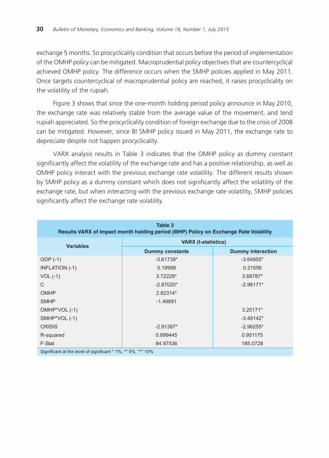
30 Bulletin of Monetary, Economics and Banking, Volume 18, Number 1, July 2015
exchange 5 months. So procyclicality condition that occurs before the period of implementation of the OMHP policy can be mitigated. Macroprudential policy objectives that are countercyclical achieved OMHP policy. The difference occurs when the SMHP policies applied in May 2011. Once targets countercyclical of macroprudential policy are reached, it raises procyclicality on the volatility of the rupiah.
Figure 3 shows that since the one-month holding period policy announce in May 2010, the exchange rate was relatively stable from the average value of the movement, and tend rupiah appreciated. So the procyclicality condition of foreign exchange due to the crisis of 2008 can be mitigated. However, since BI SMHP policy issued in May 2011, the exchange rate to depreciate despite not happen procyclicality.
VARX analysis results in Table 3 indicates that the OMHP policy as dummy constant significantly affect the volatility of the exchange rate and has a positive relationship, as well as OMHP policy interact with the previous exchange rate volatility. The different results shown by SMHP policy as a dummy constant which does not significantly affect the volatility of the exchange rate, but when interacting with the previous exchange rate volatility, SMHP policies significantly affect the exchange rate volatility.
�������������������������������������������������������������������������������������������
��������������������������
��������
��������������
��������
�
����
����
�������������
�������������
������
���������
������
���������������
������������������������������������������������������������
�������������������
���������
�������
��������
���������
��������
��������
���������
��������
��������
���������
�������
��������
���������
��������
���������
���������
��������
��������
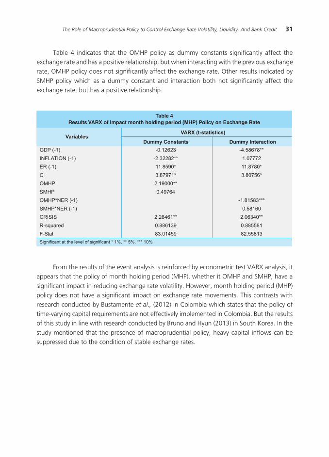
31The Role of Macroprudential Policy to Control Exchange Rate Volatility, Liquidity, And Bank Credit
From the results of the event analysis is reinforced by econometric test VARX analysis, it appears that the policy of month holding period (MHP), whether it OMHP and SMHP, have a significant impact in reducing exchange rate volatility. However, month holding period (MHP) policy does not have a significant impact on exchange rate movements. This contrasts with research conducted by Bustamente et al., (2012) in Colombia which states that the policy of time-varying capital requirements are not effectively implemented in Colombia. But the results of this study in line with research conducted by Bruno and Hyun (2013) in South Korea. In the study mentioned that the presence of macroprudential policy, heavy capital inflows can be suppressed due to the condition of stable exchange rates.
��������������������������������������������������������������������������������
��������������������������
��������
��������������
�������
�
����
����
�������������
�������������
������
���������
������
���������������
������������������������������������������������������������
�������������������
��������
����������
��������
��������
���������
�������
���������
��������
��������
����������
�������
��������
��������
�����������
�������
���������
��������
��������
Table 4 indicates that the OMHP policy as dummy constants significantly affect the exchange rate and has a positive relationship, but when interacting with the previous exchange rate, OMHP policy does not significantly affect the exchange rate. Other results indicated by SMHP policy which as a dummy constant and interaction both not significantly affect the exchange rate, but has a positive relationship.
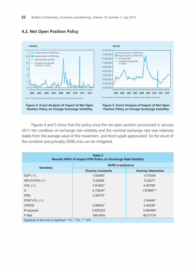
32 Bulletin of Monetary, Economics and Banking, Volume 18, Number 1, July 2015
4.2. Net Open Position Policy
Figure 4. Event Analysis of Impact of Net Open Position Policy on Foreign Exchange Volatility
Figure 5. Event Analysis of Impact of Net Open Position Policy on Foreign Exchange Volatility
Figures 4 and 5 show that the policy since the net open position announced in January 2011 the condition of exchange rate volatility and the nominal exchange rate was relatively stable from the average value of the movement, and tend rupiah appreciated. So the result of the condition procyclicality 2008 crisis can be mitigated.
��������������������������������������������������������������������
��������������������������
��������
��������������
��������
�
���
������������
������
���������
������
���������������
������������������������������������������������������������
�������������������
��������
�������
��������
��������
��������
��������
��������
��������
��������
�������
��������
����������
��������
��������
��������
��������
�
�
�
�
�
��
��
������ ��� ������ ��� ������ ��� ������ ��� ������ ��� ������ ��� ������ ��� ������ ��� ������ ���
���� ���� ���� ���� ���� ���� ���� ���� ����
������������������������
�����������������������������������������
��������������������������
����������������������������
����������������������������������������������������������������������������������
���������� ������
���� ���� ���� ���� ���� ���� ���� ���� ����
�������������������������������������������������������������������������������������������������
����������������������������������������������������������������������������������
���������
���������
���������
���������
����������
����������
����������
����������
����������
����������
��������� ��������� ��������� ��������� ��������� ��������� ��������� ��������� ������ ���
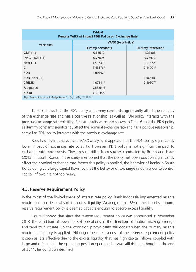
33The Role of Macroprudential Policy to Control Exchange Rate Volatility, Liquidity, And Bank Credit
Table 5 shows that the PDN policy as dummy constants significantly affect the volatility of the exchange rate and has a positive relationship, as well as PDN policy interacts with the previous exchange rate volatility. Similar results were also shown in Table 6 that the PDN policy as dummy constants significantly affect the nominal exchange rate and has a positive relationship, as well as PDN policy interacts with the previous exchange rate.
Results of event analysis and VARX analysis, it appears that the PDN policy significantly lower impact of exchange rate volatility. However, PDN policy is not significant impact to exchange rate movements. These results differ from studies conducted by Bruno and Hyun (2013) in South Korea. In the study mentioned that the policy net open position significantly affect the nominal exchange rate. When this policy is applied, the behavior of banks in South Korea doing very large capital flows, so that the behavior of exchange rates in order to control capital inflows are not too heavy.
4.3. Reserve Requirement Policy
In the midst of the limited space of interest rate policy, Bank Indonesia implemented reserve requirement policies to absorb the excess liquidity. Wearing ratio of 8% of the deposits amount, reserve requirement policy is deemed capable enough to absorb excess liquidity.
Figure 6 shows that since the reserve requirement policy was announced in November 2010 the condition of open market operations in the direction of motion moving average and tend to fluctuate. So the condition procyclicality still occurs when the primary reserve requirement policy is applied. Although the effectiveness of the reserve requirement policy is seen as less effective due to the excess liquidity that has high capital inflows coupled with large and reflected in the operating position open market was still rising, although at the end of 2011, his condition declined.
���������������������������������������������������������
��������������������������
��������
��������������
��������
�
���
������������
������
���������
������
���������������
������������������������������������������������������������
�������������������
�������
�������
��������
��������
��������
��������
��������
��������
�������
�������
��������
��������
��������
��������
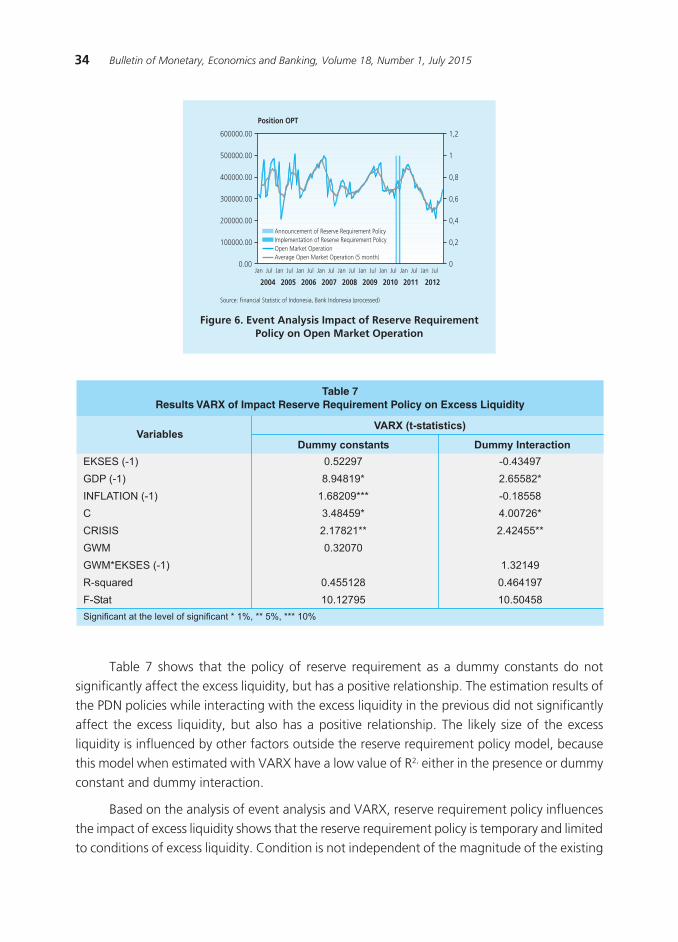
34 Bulletin of Monetary, Economics and Banking, Volume 18, Number 1, July 2015
Table 7 shows that the policy of reserve requirement as a dummy constants do not significantly affect the excess liquidity, but has a positive relationship. The estimation results of the PDN policies while interacting with the excess liquidity in the previous did not significantly affect the excess liquidity, but also has a positive relationship. The likely size of the excess liquidity is influenced by other factors outside the reserve requirement policy model, because this model when estimated with VARX have a low value of R2, either in the presence or dummy constant and dummy interaction.
Based on the analysis of event analysis and VARX, reserve requirement policy influences the impact of excess liquidity shows that the reserve requirement policy is temporary and limited to conditions of excess liquidity. Condition is not independent of the magnitude of the existing
Figure 6. Event Analysis Impact of Reserve Requirement Policy on Open Market Operation
Position OPT
����������������������������������������������������������������������������
��������������������������
����������
��������
��������������
�
������
���
��������������
���������
������
���������������
������������������������������������������������������������
�������������������
�������
��������
����������
��������
���������
�������
��������
��������
��������
��������
��������
��������
���������
�������
��������
��������
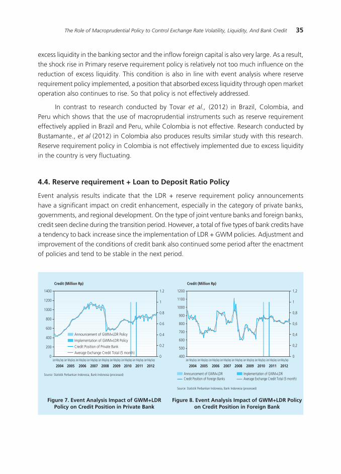
35The Role of Macroprudential Policy to Control Exchange Rate Volatility, Liquidity, And Bank Credit
excess liquidity in the banking sector and the inflow foreign capital is also very large. As a result, the shock rise in Primary reserve requirement policy is relatively not too much influence on the reduction of excess liquidity. This condition is also in line with event analysis where reserve requirement policy implemented, a position that absorbed excess liquidity through open market operation also continues to rise. So that policy is not effectively addressed.
In contrast to research conducted by Tovar et al., (2012) in Brazil, Colombia, and Peru which shows that the use of macroprudential instruments such as reserve requirement effectively applied in Brazil and Peru, while Colombia is not effective. Research conducted by Bustamante., et al (2012) in Colombia also produces results similar study with this research. Reserve requirement policy in Colombia is not effectively implemented due to excess liquidity in the country is very fluctuating.
4.4. Reserve requirement + Loan to Deposit Ratio Policy
Event analysis results indicate that the LDR + reserve requirement policy announcements have a significant impact on credit enhancement, especially in the category of private banks, governments, and regional development. On the type of joint venture banks and foreign banks, credit seen decline during the transition period. However, a total of five types of bank credits have a tendency to back increase since the implementation of LDR + GWM policies. Adjustment and improvement of the conditions of credit bank also continued some period after the enactment of policies and tend to be stable in the next period.
Figure 7. Event Analysis Impact of GWM+LDRPolicy on Credit Position in Private Bank
Figure 8. Event Analysis Impact of GWM+LDR Policy on Credit Position in Foreign Bank
�
���
���
���
���
����
����
����
�
���
���
���
���
�
���
������������������������������
��������������������������������
�������������������������������
���������������������������������������
��������� ��� ������ ��� ������ ��� ������ ��� ������ ��� ������ ��� ������ ��� ������ ���������
���� ���� ���� ���� ���� ���� ���� ���� ����
�������������������
�����������������������������������������������������������������
���
���
���
���
���
���
����
����
����
�
���
���
���
���
�
���
����������������������� ��������������������������������������������������������� ���������������������������������������
���� ���� ���� ���� ���� ���� ���� ���� ����
�������������������
�����������������������������������������������������������������
��� ������ ��� ������ ��� ������ ��� ������ ��� ������ ��� ������ ��� ������ ��� ������ ���������

36 Bulletin of Monetary, Economics and Banking, Volume 18, Number 1, July 2015
Figure 9. Event Analysis Impact of GWM+LDR Policyon Credit Position in Regional Development Bank
Figure 11. Event Analysis Impact of GWM+LDR Policy on Credit Position in Joint Venture Bank
Figure 10. Event Analysis Impact of GWM+LDR Policy on Credit Position in Government Bank
0
0.2
0.4
0.6
0.8
1
1.2
0
200
400
600
800
1000
1200
Jan-
04Ju
n-04
Nov-
04Ap
r-05
Sep-
05Fe
b-06
Jul-0
6De
c-06
May
-07
Oct
-07
Mar
-08
Aug-
08Ja
n-09
Jun-
09No
v-09
Apr-1
0Se
p-10
Feb-
11Ju
l-11
Dec-
11M
ay-1
2O
ct-1
2Source: Statistik Perbankan Indonesia, Bank Indonesia (processed)
Announcement of GWM+LDR Policy Implementation of GWM+LDR Policy
Credit Position of Regional Development Bank Average Exchange Credit Total (5 month)
0
0.2
0.4
0.6
0.8
1
1.2
0
200
400
600
800
1000
Jan-
04Ap
r-04
Jul-0
4O
ct-0
4Ja
n-05
Apr-0
5Ju
l-05
Oct
-05
Jan-
06Ap
r-06
Jul-0
6O
ct-0
6Ja
n-07
Apr-0
7Ju
l-07
Oct
-07
Jan-
08Ap
r-08
Jul-0
8O
ct-0
8Ja
n-09
Apr-0
9Ju
l-09
Oct
-09
Jan-
10Ap
r-10
Jul-1
0O
ct-1
0Ja
n-11
Apr-1
1Ju
l-11
Oct
-11
Jan-
12Ap
r-12
Jul-1
2O
ct-1
2
Source: Statistik Perbankan Indonesia, Bank Indonesia (processed)
Announcement of GWM+LDR Policy Implementation of GWM+LDR Policy
Credit Position of Government Bank Average Exchange Credit Total (5 month)
���
���
���
���
����
����
����
�
���
���
���
���
�
���
������ ��� ������ ��� ������ ��� ������ ��� ������ ��� ������ ��� ������ ��� ������ ��� ������ ���
���� ���� ���� ���� ���� ���� ���� ���� ����
������������������������������ ��������������������������������
������������������������������������ ���������������������������������������
�����������������������������������������������������������������
After the issuance of the policy reserve requirement + LDR, as expected, the impact of this policy is contractionary in the beginning. This is evident from the decline in credit growth in 3 months in each type of bank after implementation of the policy reserve requirement + LDR. Then, in the following months, the credit growth back to normal and even continue to rise. Although based on the Figure, the results indicate that the implementation of GWM + LDR associated with a reduction in credit growth, but it can also be caused by synchronization between tightening reserve requirement policy with the increase in the BI rate. Therefore, event analysis is not possible to separate the effects of truly comes from or is derived from the reserve requirement policy and shock interest rate policy.
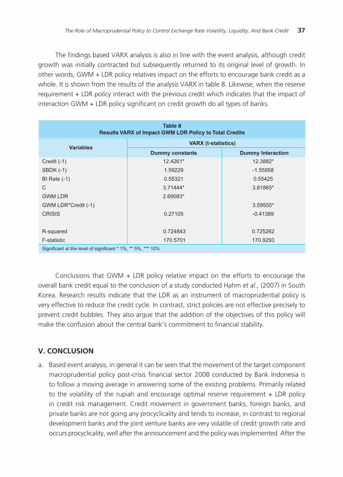
37The Role of Macroprudential Policy to Control Exchange Rate Volatility, Liquidity, And Bank Credit
The findings based VARX analysis is also in line with the event analysis, although credit growth was initially contracted but subsequently returned to its original level of growth. In other words, GWM + LDR policy relatives impact on the efforts to encourage bank credit as a whole. It is shown from the results of the analysis VARX in table 8. Likewise, when the reserve requirement + LDR policy interact with the previous credit which indicates that the impact of interaction GWM + LDR policy significant on credit growth do all types of banks.
�������������������������������������������������������������
��������������������������
�����������
���������
������������
�
�������
�������������������
������
���������
�����������
���������������
������������������������������������������������������������
�������������������
��������
�������
�������
��������
��������
�������
���������
���������
��������
��������
�������
��������
��������
��������
��������
��������
Conclusions that GWM + LDR policy relative impact on the efforts to encourage the overall bank credit equal to the conclusion of a study conducted Hahm et al., (2007) in South Korea. Research results indicate that the LDR as an instrument of macroprudential policy is very effective to reduce the credit cycle. In contrast, strict policies are not effective precisely to prevent credit bubbles. They also argue that the addition of the objectives of this policy will make the confusion about the central bank’s commitment to financial stability.
V. CONCLUSION
a. Based event analysis, in general it can be seen that the movement of the target component macroprudential policy post-crisis financial sector 2008 conducted by Bank Indonesia is to follow a moving average in answering some of the existing problems. Primarily related to the volatility of the rupiah and encourage optimal reserve requirement + LDR policy in credit risk management. Credit movement in government banks, foreign banks, and private banks are not going any procyclicality and tends to increase, in contrast to regional development banks and the joint venture banks are very volatile of credit growth rate and occurs procyclicality, well after the announcement and the policy was implemented. After the
38 Bulletin of Monetary, Economics and Banking, Volume 18, Number 1, July 2015
announcement and implementation of OMHP and PDN policies does not occur procyclicality on exchange rate volatility and the foreign exchange rate, but after implemented SMHP policies occur procyclicality on exchange rate volatility. The level of liquidity banks not occur procyclicality in the it movement after the announcement and application of the primary reserve requirement policy.
b. Macroprudential policy which has been pursued by the Bank of Indonesia most effective. Based on the results of the econometric tests using VARX showed that the level of exchange rate volatility decreased after the implementation of one month holding, six month holding, and net open position policy. However, the nominal exchange rate, these policies are not effective. Although the aggregated reserve requirement + LDR policy effective raising credit bank, but to foreign and joint venture banks is not effective. Furthermore, the impact of primary reserve requirement policy is very limited in the economy given the lower liquidity at the same time the flow of foreign capital into very heavy.
Based on the analysis of the first research goal is to analyze the movement of the target macroprudential policy instruments before and after the policy is implemented, then the appropriate policy recommendations to be implemented is a policy that provides a disincentive for short-term capital flows. Liabilities hedging on capital flows are steps that can be applied to extend the period of capital inflows. In addition, restrictions on reserve requirement bank needs to be studied further because after the policy being applicable there are still some issues regarding bank liquidity tends to be unstable and the growth rate of excess liquidity is higher.
While based on the results of the analysis of the purpose of the second study is to analyze the effectiveness of policy instruments macroprudential (month holding period, net open position, reserve requirement and reserve requirement + LDR ) which has been implemented in Indonesia, the paradigm that monetary policy needs to be supported by macroprudential policy consequences can not be the separation of these two policies in different institutions in order to operate effectively. In this context, if the banking supervision function is separated from Bank Indonesia, macroprudential policy framework can’t be avoided and must involve two institutions, namely BI and the OJK (Otoritas Jasa Keuangan / Financial Service Authority). The best course, BI is mandated macroprudential while the OJK mandated microprudensial. In this context, BI plays a role in the risk oversight of the financial system as a whole and can perform regulations and actions that may lead to systemic risk.
Some financial reform agenda over the long term needs to be done to reduce procyclicality financial system in Indonesia. First, the development of a more diversified financial system by developing non-bank financial markets, such as corporate bonds should be encouraged so that the company does not depend on the bank. Secondly, the role of foreign banks that need to be clearly defined. Third, the banking supervision should also be countercyclical to do a more intensive examination when grown very high credit growth in line with the period of economic expansion.
39The Role of Macroprudential Policy to Control Exchange Rate Volatility, Liquidity, And Bank Credit
REFERENCES
Agung, Juda. 2010. Mengintegrasikan Kebijakan Moneter dan Makroprudensial: Menuju Paradigma Baru Kebijakan Moneter di Indonesia Pasca Krisis Global. Working Paper, No. 07. Bank Indonesia.
Angelini, Paolo, Stefano Neri , dan Fabio Panetta. 2012. Monetary and Macroprudential Policies. Working Paper Series, No 1449, European Central Bank, Juli.
Arnold, Bruce, Claudio Borio, Luci Ellis, dan Fariborz Moshirian. 2012. Syatemic Risk, Macroprudential Policy Frameworks, Monitoring Financial System, and the Evolution of Capital Adequacy. Journal of Banking and Finance, vol.36: 3125-3132.
Arregui, Nicolas, Jaromir Banes, Ivo Krznar, Srobona Mitra, dan Andre Oliveira Santos. 2013. Evaluating the Net Benefit of Macroprudential Policy: A Cookbook. IMF Working Paper, WP/13/167.
Bank of England. 2009. The Role of Macroprudential Policy. A Discussion Paper, November.
Bank of England. 2011. Instrument of Macroprudential Policy. A Discussion Paper, Desember
Beau, Denis, Laurent Clerc dan Benoit Mojon. 2012. Macro-Prudential Policy and the Conduct of Monetary Policy. Banque de France Working Paper, No.390, Juli.
Bierens, Herman J.. 2004. VAR Models with Exogenous Variables.
http://www.econ.psu.edu/~hbierens/EasyRegTours/VAR_Tourfiles/VARX.PDF, diunduh Februari 2014
Biorn, Erik. 2011. Estimation of ARX and VARX Models by ML. Advanced Econometrics-Time
Series, Lecture note No. 6, Februari.
Bruno, Valentina dan Hyun Song Shin. 2013. Assessing Macroprudential Policies: Case of Korea. Prepared for the Symposium Issue of the Scandinavian Journal of Economics on
Capital Flow, April.
Buncic, Daniel, dan Martin Melecky. 2013. Macroprudential Stress Testing of Credit Risk: A Practical Approach for Policy Makers. Journal of Financial Stabilty, No. 9: 347-370.
Bustamante, C., Gonzales, A., dan Perez, J. 2012. Macroprudential Policy, External Shocks and Financial Intermediation on a Small Open Economy. Borradores de Economica, No. 716I.
Claessens, Stijn dan Swati R. Ghosh. 2012. Macro-Prudential Policies: Lesson for and from Emerging Markets. Prepared for the East-West Center and the Korea Development Institute
Conference, Juli.
Claessens, Stijn, Swati R. Ghosh, dan Roxana Mihet. 2012. Macro-Prudential Policies to Mitigate Financial System Vulnerabilities. Prepared for the NIPFP-DEA-JIMF conference Rajasthan, India, November.

40 Bulletin of Monetary, Economics and Banking, Volume 18, Number 1, July 2015
Clemment, P. 2010. The Term “Macroprudential”: Origins and Evolution. Quarterly Review, Bank for International Settlement, Maret.
Committee on the Global Financial System. 2010. Macroprudential Instruments and Frameworks: A Stocktaking of Issues and Experiences. CGFS Papers, No. 38. Bank for International Settlements, Mei.
Committee on the Global Financial System. 2012. Operationalising the Selection and Application of Macroprudential Instruments. CGFS Papers, No. 48. Bank for International Settlements, Desember.
Cui, Yuhu, dan Ansgar Belke. 2008. Monetary Policy Interdependence between the ECB and The Fed: VARX Model versus VEC Model. International Conference on Applied Economics, Mei.
Delgado, Fernando L., dan Mynor Meza. 2011. Developments in Financial Supervision and the use of Macroprudential Measures in Central America. IMF Working Paper, WP/11/299, Desember.
G20 Finance Ministers and Central Bank Governors. 2011. Macroprudential Policy Tools
and Frameworks. Financial Stability Board, International Monetary Fund, dan Bank for international Settlements, Februari.
Galati, Gabriele dan Richhild Moessner. 2011. Macroprudential Policy – A Literature Review. Working Paper No. 337. Bank for International Settlements, Februari.
Gauthier, Celine, Alfred Lehar, dan Moez Souissi. 2012. Macroprudential Capital Requirements and Systemic Risk. Journal of Financial Intermediation, No. 21: 594-618.
Gersbach, Hans, dan Jean-Charles Rochet. 2012. Aggregate Investment Externalities and Macroprudential Regulation. Journal of Money, Credit, and Banking, Vol. 44, No. 2: 73-109.
Hahm, Joon-Ho, Frederic S. Mishkin, Hyun Song Shin, dan Kwanho Shin. 2011. Macroprudential Policies in Open Emerging Economies. Asia Economic Policy Conference. Februari.
Horvath, Csilla, Peter S.H. Leeflang, Jaap E. Wieringa, Dick R. Wittink. 2005. Competitive Reaction and Feedback Effects Based on VARX Models of Pooled Store Data. International
Journal of Research in Marketing 22: 415-426.
International Monetary Fund. 2011. Macroprudential Policy: An Organizing Framework. Prepared
by the Monetary and Capital Markets Department.
International Monetary Fund. 2013. Key Aspects of Macroprudential Policy. Juni.
Lim, C., F. Columba, A. Costa, P. Kongsamut, A. Otani, M. Saiyid, T. Wezel, dan X. Wu. 2011. Macroprudential Policy: What Instruments and How to Use Them? Lessons from Country Experiences. IMF Working Paper, WP/11/238, Oktober.

41The Role of Macroprudential Policy to Control Exchange Rate Volatility, Liquidity, And Bank Credit
Lima, Diana, Paul Levine, dan Joseph Pearlman. 2012. Optimal Macro-Prudential and Monetary
Policy. University of Surrey, Agustus.
Mendicino, Caterina. 2012. Collateral Requirements: Macroeconomic Fluctuations and Macroprudential Policy. Working Paper No. 11, Banco de Portugal, April.
Milne, Alistair. 2009. Macro-prudential Policy: Is It Really So New?. Draft Paper for Oxford
Review of Economic Policy. Desember.
Peraturan Bank Indonesia No.12/10 /PBI/2010 Tentang Perubahan Ketiga atas Peraturan Bank Indonesia. Nomor 5/13/PBI/2003
Peraturan Bank Indonesia Nomor 15/7/ PBI /2013 Tentang Perubahan Kedua Atas
Peraturan Bank Indonesia Nomor 12/19/ PBI /2010 Tentang Giro Wajib Minimum Bank Umum Pada Bank Indonesia Dalam Rupiah Dan Valuta Asing.
Peraturan Bank Indonesia Nomor: 12/19/ PBI /2010 Tentang Giro Wajib Minimum Bank Umum Pada Bank Indonesia Dalam Rupiah Dan Valuta Asing
Peraturan Bank Indonesia Nomor: 5/13/PBI/2003 Tentang Posisi Devisa Neto Bank Umum
Peraturan Bank Indonesia. Nomor: 12/ 11 / PBI /2010 Tentang. Operasi Moneter
Progress Report to G20. 2011. Macroprudential Policy Tools and Frameworks. Financial Stability Board, International Monetary Fund, Bank for International Settlements, Oktober.
Quint, Dominic dan Pau Rabanal. 2011. Monetary and Macroprudential Policy in an Estimated DSGE Model of the Euro Area. 12th Jacques Polak Annual Research Conference, November.
Schoenmaker, Dirk dan Peter Wierts. 2011. Macroprudential Policy: The Need for a Coherent Policy Framework. Duisenberg School Finance Policy Paper Series, No. 13, Juli.
Tovar, Camilo E., Mercedes Garcia-Escribano, and Mercedes Vera Martin. 2012. Credit Growth and the Effectiveness of Reserve Requirements and Other Macroprudential Instruments in Latin America. IMF Working Paper, WP/12/142, Juni.
Utari, Diah dan Arimurti, Trinil. 2011. A Macro-Prudential Assessment For Indonesia. Bank Indonesia.
http://www.seacen.org/file/file/RP88/framework%20chap3.pdf.
diunduh Desember 2013.
Working Group G-30. 2010. Enhancing Financial Stability and Resilience: Macroprudential Policy, Tools, and Systems for the Future. Working Paper G-30.

42 Bulletin of Monetary, Economics and Banking, Volume 18, Number 1, July 2015
This page intentionally left blank
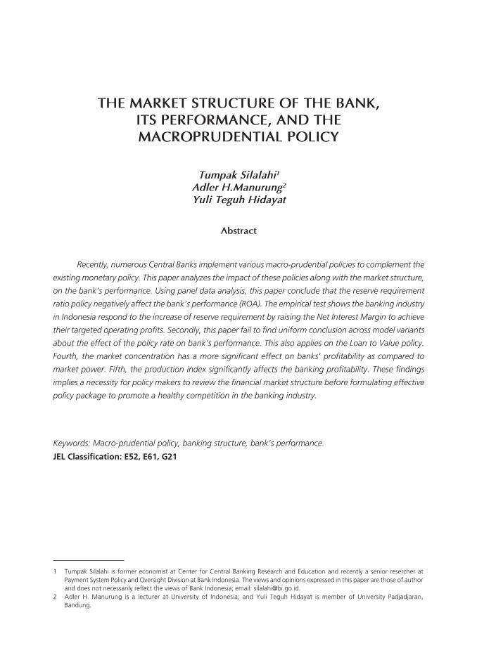
43The Market Structure of The Bank, Its Performance, and The Macroprudential Policy
THE MARKET STRUCTURE OF THE BANK,ITS PERFORMANCE, AND THEMACROPRUDENTIAL POLICY
Tumpak Silalahi1
Adler H.Manurung2
Yuli Teguh Hidayat
Recently, numerous Central Banks implement various macro-prudential policies to complement the
existing monetary policy. This paper analyzes the impact of these policies along with the market structure,
on the bank’s performance. Using panel data analysis, this paper conclude that the reserve requirement
ratio policy negatively affect the bank’s performance (ROA). The empirical test shows the banking industry
in Indonesia respond to the increase of reserve requirement by raising the Net Interest Margin to achieve
their targeted operating profits. Secondly, this paper fail to find uniform conclusion across model variants
about the effect of the policy rate on bank’s performance. This also applies on the Loan to Value policy.
Fourth, the market concentration has a more significant effect on banks’ profitability as compared to
market power. Fifth, the production index significantly affects the banking profitability. These findings
implies a necessity for policy makers to review the financial market structure before formulating effective
policy package to promote a healthy competition in the banking industry.
Abstract
Keywords: Macro-prudential policy, banking structure, bank’s performance.
JEL Classification: E52, E61, G21
1 Tumpak Silalahi is former economist at Center for Central Banking Research and Education and recently a senior resercher at Payment System Policy and Oversight Division at Bank Indonesia. The views and opinions expressed in this paper are those of author and does not necessarily reflect the views of Bank Indonesia; email: [email protected].
2 Adler H. Manurung is a lecturer at University of Indonesia; and Yuli Teguh Hidayat is member of University Padjadjaran, Bandung.

44 Bulletin of Monetary, Economics and Banking, Volume 18, Number 1, July 2015
I. INTRODUCTION
The objective of the macro-prudential instruments is to stabilize the financial systems. This macro-prudential policy may affect the profitability of the bank, and its effectiveness may subject to the market structure of the banking industry. This should be evident in emerging countries like Indonesia with their highly segmented banking market structure.
For the largest five Southeast Asian countries (ASEAN-5), Indonesia has the highest net interest margin (NIM), indicating the Indonesian banks are relatively less efficient than the other ASEAN countries. For Indonesia, this particular condition will potentially affect the effectiveness of the policies. The performance of Indonesian banks relative to other banks in the Southeast Asia are depicted on the Figure 1.
Figure 1. Average Net Interest margin top 10 Bank’s in ASEAN-5
���
���
���
���
���
���
���
���
�
��� ������ ��� ��� ��� ���
������ ���
��� ��� ��� ��� ��� ��� ������ ��� ���
���� ���� ���� ���� ���� ���� ���� ���� ���� ����
�������������������������������������������������������������������
��������� �������� ��������� ��������� ��������
The research on macro prudential regulation and its implementation is relatively new and in fact there is significant gap between the theoretical and the empirical research on this subject. This paper will review and analyze the impact of macro-prudential policies on the performance of the commercial banks in Indonesia. This paper will also identify if the market power or the market concentration is more prominent on the commercial bank profitability. Furthermore, this paper will analyze the interaction between the market power or the market concentration and the macro prudential policy in conjunction with the profitability of commercial banks in Indonesia.
Basically, this paper employ econometric model on quarterly commercial bank data from 2005 until 2014. We took the advantage of the longitudinal data and use the panel data estimation. We confront the estimated model with descriptive analysis and the existing studies.
45The Market Structure of The Bank, Its Performance, and The Macroprudential Policy
The next section of this paper outlines the theory and related empirical literature. Section three discusses the methodology including the empirical model and data used on estimation. Section four provides the result of estimation and its analysis, while section five presents the conclusion, and will close this paper.
II. THEORY
Unlike the production of goods at micro level, the production of services in banking industry is more complicated. Xavier et al (1998, p.1) defines the operation of the bank as a financial institution that guarantees loans and accepts deposits from the public. While, Rose and Hudgins (2005) defines bank more comprehensively by the economic functions it serves and the services it offers to customers and as well as by the legal basis of its existence.
Several literatures explained the level of the banking productivity by diagnosing their balance sheets; this includes Xavier et.al (2008), Mankiw (1986), and Mishkin (2010). Simplified balance sheet of the bank is below,
��������������������������������
������
������������
��������
���������������������
������������
������
On the assets side, the reserve of the bank, Rit is highly related to the macroprudential
policy. It is calculated as the difference between the volume of deposits received by the banks and the volume of loans disbursed (D
it – L
it). Reserve of the bank can be classified into two types;
statutory reserves (SR) and voluntary reserve placed in the interbank market (Mt),
Monetary authorities generally require commercial banks to keep a portion of the public funds as statutory reserves (reserve requirement) and deposit it in the central bank either in cash or securities. The amount of the reserve requirement set by monetary authority affect the ability of banks to lend, which may affect the performance of the bank.
The simple Monti-Klein model is helpful in explaining the market structure, the conduct and the performance of the banking industry. Other theories in explaining the correlation between performance and concentration are Hypothesis of Structure Conduct Performance (SCP) and Hypothesis of Relative Market Power (RMP). The traditional SCP Hypothesis stated that the level of the bank profitability correlates to the level of market domination (or market
Rit= + (1)
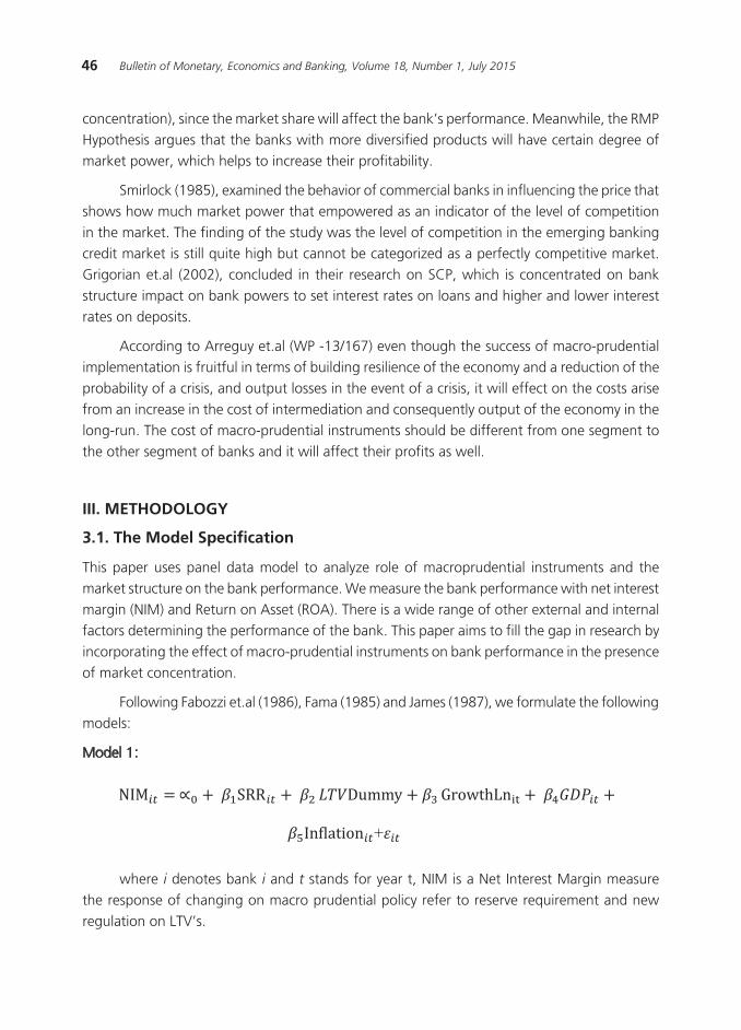
46 Bulletin of Monetary, Economics and Banking, Volume 18, Number 1, July 2015
concentration), since the market share will affect the bank’s performance. Meanwhile, the RMP Hypothesis argues that the banks with more diversified products will have certain degree of market power, which helps to increase their profitability.
Smirlock (1985), examined the behavior of commercial banks in influencing the price that shows how much market power that empowered as an indicator of the level of competition in the market. The finding of the study was the level of competition in the emerging banking credit market is still quite high but cannot be categorized as a perfectly competitive market. Grigorian et.al (2002), concluded in their research on SCP, which is concentrated on bank structure impact on bank powers to set interest rates on loans and higher and lower interest rates on deposits.
According to Arreguy et.al (WP -13/167) even though the success of macro-prudential implementation is fruitful in terms of building resilience of the economy and a reduction of the probability of a crisis, and output losses in the event of a crisis, it will effect on the costs arise from an increase in the cost of intermediation and consequently output of the economy in the long-run. The cost of macro-prudential instruments should be different from one segment to the other segment of banks and it will affect their profits as well.
III. METHODOLOGY
3.1. The Model Specification
This paper uses panel data model to analyze role of macroprudential instruments and the market structure on the bank performance. We measure the bank performance with net interest margin (NIM) and Return on Asset (ROA). There is a wide range of other external and internal factors determining the performance of the bank. This paper aims to fill the gap in research by incorporating the effect of macro-prudential instruments on bank performance in the presence of market concentration.
Following Fabozzi et.al (1986), Fama (1985) and James (1987), we formulate the following models:
Model 1:
NIM SRR GrowthLn
In�lation +
where i denotes bank i and t stands for year t, NIM is a Net Interest Margin measure the response of changing on macro prudential policy refer to reserve requirement and new regulation on LTV’s.
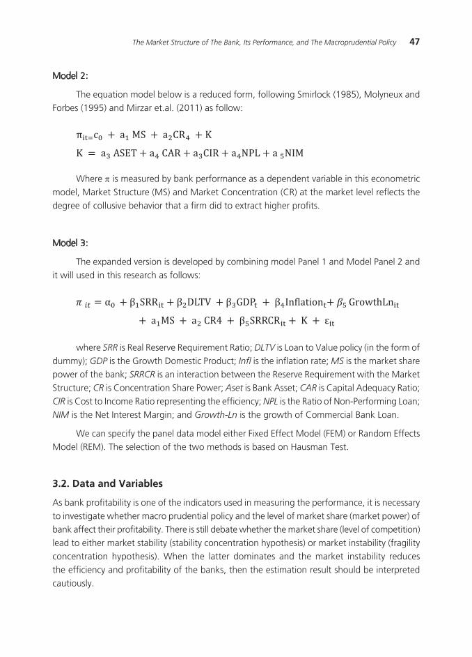
47The Market Structure of The Bank, Its Performance, and The Macroprudential Policy
Model 2:
The equation model below is a reduced form, following Smirlock (1985), Molyneux and Forbes (1995) and Mirzar et.al. (2011) as follow:
π c CR
NIM
Where π is measured by bank performance as a dependent variable in this econometric model, Market Structure (MS) and Market Concentration (CR) at the market level reflects the degree of collusive behavior that a firm did to extract higher profits.
Model 3:
The expanded version is developed by combining model Panel 1 and Model Panel 2 and it will used in this research as follows:
SRR GDP In�lation GrowthLn
SRRCR
where SRR is Real Reserve Requirement Ratio; DLTV is Loan to Value policy (in the form of dummy); GDP is the Growth Domestic Product; Infl is the inflation rate; MS is the market share power of the bank; SRRCR is an interaction between the Reserve Requirement with the Market Structure; CR is Concentration Share Power; Aset is Bank Asset; CAR is Capital Adequacy Ratio; CIR is Cost to Income Ratio representing the efficiency; NPL is the Ratio of Non-Performing Loan; NIM is the Net Interest Margin; and Growth-Ln is the growth of Commercial Bank Loan.
We can specify the panel data model either Fixed Effect Model (FEM) or Random Effects Model (REM). The selection of the two methods is based on Hausman Test.
3.2. Data and Variables
As bank profitability is one of the indicators used in measuring the performance, it is necessary to investigate whether macro prudential policy and the level of market share (market power) of bank affect their profitability. There is still debate whether the market share (level of competition) lead to either market stability (stability concentration hypothesis) or market instability (fragility concentration hypothesis). When the latter dominates and the market instability reduces the efficiency and profitability of the banks, then the estimation result should be interpreted cautiously.

48 Bulletin of Monetary, Economics and Banking, Volume 18, Number 1, July 2015
������������������������
�� �������������
�
�
�
�
�
�
�
�
�
��
��
��
��������� ����������� �������������
������������
�����������
�����������
������������
�������������
�����
����
������������
������������
���������������
�����������
������������
������
�����������
���������
���������
����������������������������������������
����������������������������������������������
�����������������������������������������������
������������������������
������������������������������������������������
������������������������������������
�������������������
�����������������������������������������
����������
����������������������������������
������������������������������������������������
����������������������������������
�������������������
����������������������������������������
���������������
����
�������������
��
��
��
����������
��
��
��
��
��
���
���
�
�
�
�
���
�
�
�
�
�
�
�
The data are obtained from Bank Indonesia (Indonesian Banking Directory), Bank Scope and the data of International Financial Statistics (IFS). The accuracy of data can be trusted since the commercial banks have the obligation to submit data of the highest quality, where failure to comply could result in penalty charges.
By checking the data so the sample of bank choice becomes 98 banks out of 109 commercial bank figure out of 89.9% of total bank population. The descriptive statistic of the data gathered and variable used are presented in table 3.
Based on the table above, the variables can be classified into five groups, where Bank Performance as dependent variable is the first group. The second group is market structure of the bank industry that consists of market power and Market Concentration. Subsequently, macro prudential variable consists of reserve requirement and Loan to Value (LTV’s). Internal bank characteristic consists of Capital Adequacy Ratio (CAR), Cost to Income Ratio (CIR), Non-performing Loan (NPL’S), and Loan Growth as representative of bank indictor to provide a supply of loan to market. Lastly, macroeconomic indicator is representative of external factors that influence the banking performance.
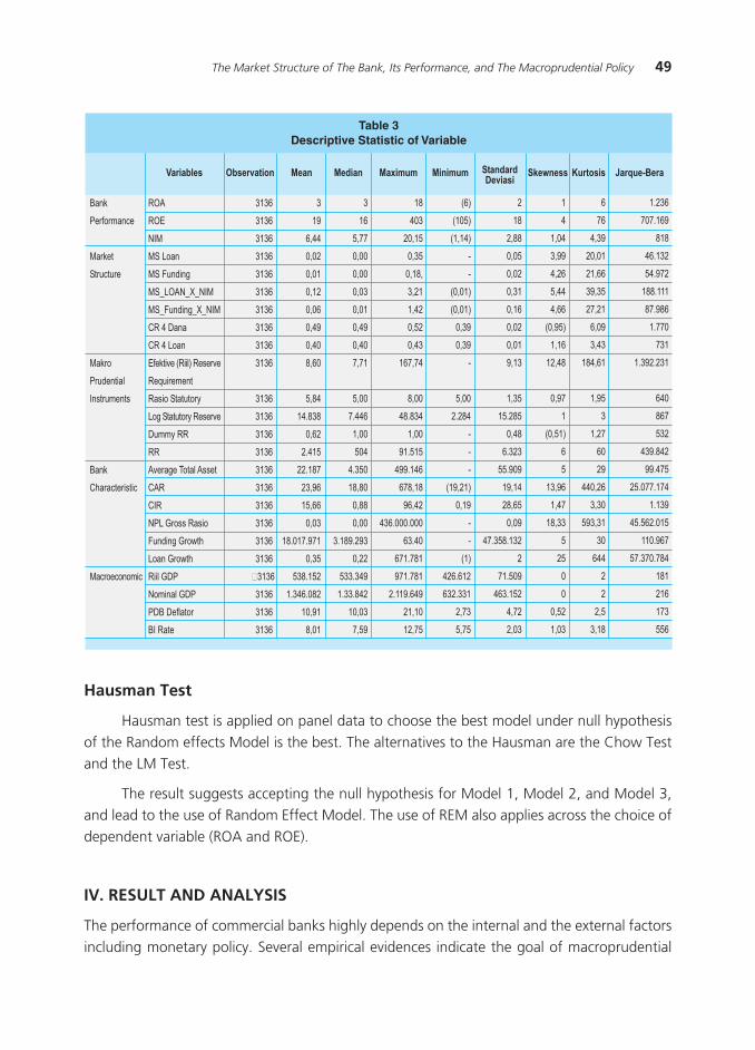
49The Market Structure of The Bank, Its Performance, and The Macroprudential Policy
Hausman Test
Hausman test is applied on panel data to choose the best model under null hypothesis of the Random effects Model is the best. The alternatives to the Hausman are the Chow Test and the LM Test.
The result suggests accepting the null hypothesis for Model 1, Model 2, and Model 3, and lead to the use of Random Effect Model. The use of REM also applies across the choice of dependent variable (ROA and ROE).
IV. RESULT AND ANALYSIS
The performance of commercial banks highly depends on the internal and the external factors including monetary policy. Several empirical evidences indicate the goal of macroprudential
����������������������������������������
���������
����
�����������
������
���������
�����
����������
�����������
����
��������������
�������������
����������� ���� ������ ������� ������� ���������������
�������� �������� �����������
���
���
���
�������
����������
�������������
����������������
���������
���������
�����������������������
�����������
���������������
���������������������
��������
��
�������������������
���
���
���������������
��������������
�����������
��������
�����������
������������
�������
����
����
����
����
����
����
����
����
����
����
����
����
����
����
����
����
����
����
����
����
�����
����
����
����
�
��
����
����
����
����
����
����
����
����
����
������
����
�����
������
�����
�����
����
����������
����
�������
���������
�����
����
�
��
����
����
����
����
����
����
����
����
����
�����
����
���
�����
�����
����
����
���������
����
�������
��������
�����
����
��
���
�����
����
�����
�����
����
����
����
������
����
������
����
������
�������
������
�����
�����������
�����
�������
�������
���������
�����
�����
���
�����
������
�
�
������
������
����
����
�
����
�����
�
�
�
�������
����
�
�
���
�������
�������
����
����
�
��
����
����
����
����
����
����
����
����
����
������
����
�����
������
�����
�����
����
����������
�
������
�������
����
����
�
�
����
����
����
����
����
������
����
�����
����
�
������
�
�
�����
����
�����
�
��
�
�
����
����
�
��
����
�����
�����
�����
�����
����
����
������
����
�
����
��
��
������
����
������
��
���
�
�
���
����
�����
�������
���
������
������
�������
������
�����
���
���������
���
���
���
�������
������
����������
�����
����������
�������
����������
���
���
���
���

50 Bulletin of Monetary, Economics and Banking, Volume 18, Number 1, July 2015
policy to stabilize the macro economy does not align with the goal of commercial banks to maximize the shareholder value. In this section, we focus our analysis on how the market structure interacts with the macro prudential policy on affecting the banks’ profitability.
4.1. The Effect of Macroprudential and Market Structure on ROA and ROE
On the Model 1 the effect of macro-prudential policy is represented by the change in ratio of reserve requirement. Based on empirical evidence, it is observed that reserve requirement ratio has significant effect on ROA of Indonesian banks. The negative coefficient on reserve requirement means that for every 1% increase in reserve requirement, ROA decreases by 0.83%. Negative sign coefficient of LTV policy shows that it has an inverse relationship with bank. Nonetheless, LTV policy has not shown big influence bank profitability since its implementation in 2012 as depicted in Model 1 that uses Fixed Effect model.
To policy makers, all these findings will assist them in simulating the effect of macro prudential policy on banks’ profit and therefore determine the maximum increase in capital reserve requirement, which can be imposed on commercial banks to avoid contagion effect. This is important to maintain financial stability of Central Bank as a whole.
However for the banks with portfolio assets consisting marketable securities such as government bond or interbank call money, their strategy in anticipating change in the macro prudential policy is by changing the composition of deposits from expensive funding sources to less expensive ones such as saving and current deposit.
A new LTV, a macro prudential instrument, regulation that requires bank to apply a minimum 30% down payment out of total financing on housing loan needs to be monitored closely as to prevent disastrous housing properties bubble.
Finding by Silalahi et.al (2012), shows that the short term growth of property prices is affected by the growth of bank lending, capital market index, interest rate, the GDP growth and the past growth in property prices from one and up three quarters lag.
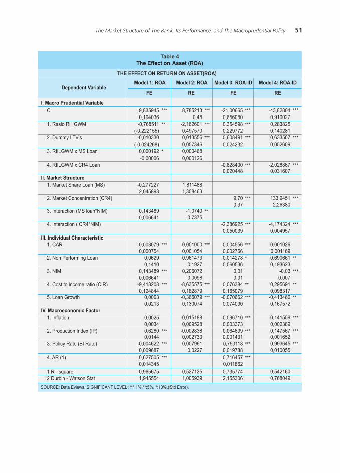
51The Market Structure of The Bank, Its Performance, and The Macroprudential Policy
��������������������������������
������������������������������������������������������������������������
����������������������������������
������������ ������������ ��������������� ���������������
�� �� �� ��������������������
�
�����������������
��������������
��������������������
���������������������
�������������������������
�����������������������������
����������������������������
�������������������������
������
����������������������
������
�����������������������������
��������������
������������
������������������������
������������������������
���������
����������������������������������
������������������������������
������������������������
��������������������
�������������������������������
��
�
���
���
���
���
���
���
�������������������������
��������������������
���������������������������
�����������������
����������������
����������������
������������
���������������������������������
������������
�������������������������
�������������������������������������������������
���
���
���
��
���
���
���
������������
�������������������������������������������������
����������������
��������������
������������������������
��������������
����������������������������������������
������������������������������������������
������
����������������
���
���
���
���
���
���
���
�
��
���
���
���
���
���
�������������������������������������������������
�����������������
��������
�����������������
��������������������������������
��������
���������������������������������
���������������������������������������������������������������������������������
���
���
���
���
���
��
���
��
��
���
���
���
�������������������������������������������������
�����������������
���������������
�����������������
��������������������������������
����������
���������������������������������
�������������������������������������������������
����������������

52 Bulletin of Monetary, Economics and Banking, Volume 18, Number 1, July 2015
4.2. The Effect of Market Structure on ROA and ROE
The degree of market shares owns by each of the four most prominent banks had a greater role in influencing their profitability compared to extent of market power that each of them had. This finding is supported by variable CR4, which has positive coefficient. This finding is in line with research done by Mirzaei et.al. (2012), Perera et.al. (2013) and Smirlock, M (1985).
There are two hypothesis related to market structure, which are Structure Conduct
Performance Hypothesis (SCP) or Relative Market Power Hypothesis (RMP). SCP hypothesis argues that market concentration has significant effect on performance of banks. However, Relative Market Power argues the capability of commercial bank to do product diversification will encourage efficiency and commercial banks can therefore achieve their optimal performance level by solely relying on their abilities to innovate on the services that they provide.
In emerging countries like Indonesia, empirical evidence shows that market concentration (CR4) has a more significant effect on banks’ profitability as compared to market power (MS) This finding is supported by the p-value of market concentration, which proves CR4 to be significant at 5% significance level while MS is not. This finding is also supported by statistic of the four largest banks by asset and loan value and similar trend is also observed when the model is expanded to include eleven of the top banks. The above findings support the data that the aggregate profit of the top 10 banks in Indonesia makes up significant portion of total profit in the country’s banking industry.
���������������������������������
���������������������������������������������������������������������������
������������������������������������
������������ ������������ ��������������� ���������������
������������������ �� ������������������������
���
���
�
���
���
�
��
�
���
���
���
���
��
���
���
�
�
�
���
�
���
���
���
�
��
���
���
���
���
���
���
���
���
���
���
��
��
�
���
�
��
���
���
���
�������������
������������
������������
������������
������������
�������������
������������
������������
������������
������������
�������������
������������
������������
�������������
��������������
������������������
������������������������
��������
�������������
���������
�����������������������������������������
�������������������������������������������
�������������
�������������
������������
������������
��������������
������������
�������������
�������������
������������
�������������������������
������������
������������
�������������
��������������
�������������
�������������
������������
������������
��������������
�������������
���������������������������������������������������
�������������
������������
������������
������������
��������������
���������
�����������������
��������������
�������������������
��������������������
��������������������
�����������
�������������������������������
���������������������������
������
����������
������
�������������
���������������������
������������
������������������������
������������������������
���������
������������������������������������
������������������������
������������������������
��������������������
������������������������������
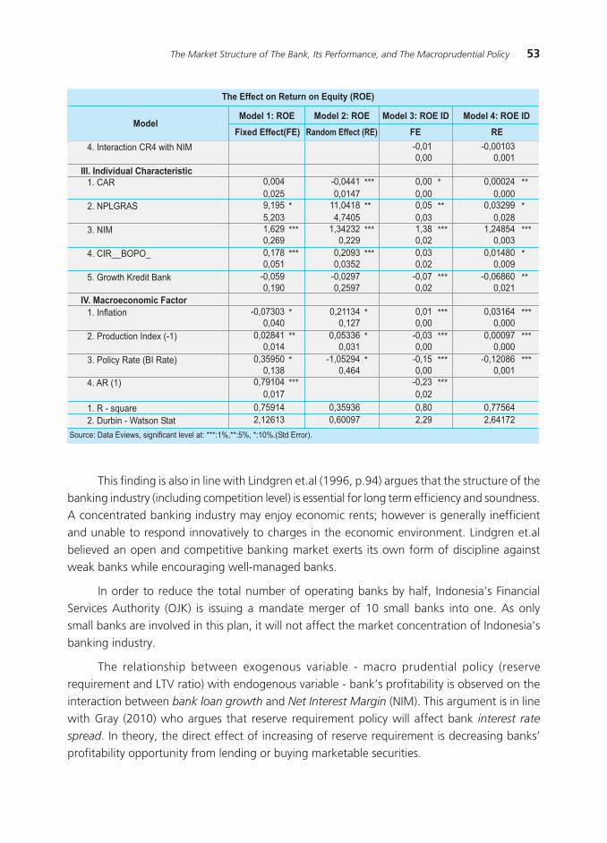
53The Market Structure of The Bank, Its Performance, and The Macroprudential Policy
This finding is also in line with Lindgren et.al (1996, p.94) argues that the structure of the banking industry (including competition level) is essential for long term efficiency and soundness. A concentrated banking industry may enjoy economic rents; however is generally inefficient and unable to respond innovatively to charges in the economic environment. Lindgren et.al believed an open and competitive banking market exerts its own form of discipline against weak banks while encouraging well-managed banks.
In order to reduce the total number of operating banks by half, Indonesia’s Financial Services Authority (OJK) is issuing a mandate merger of 10 small banks into one. As only small banks are involved in this plan, it will not affect the market concentration of Indonesia’s banking industry.
The relationship between exogenous variable - macro prudential policy (reserve requirement and LTV ratio) with endogenous variable - bank’s profitability is observed on the interaction between bank loan growth and Net Interest Margin (NIM). This argument is in line with Gray (2010) who argues that reserve requirement policy will affect bank interest rate
spread. In theory, the direct effect of increasing of reserve requirement is decreasing banks’ profitability opportunity from lending or buying marketable securities.
���������������������������������
���������������������������������������������������������������������������
������������������������������������
������������ ������������ ��������������� ���������������
������������������ �� ������������������������
���
���
�
���
���
�
��
�
���
���
���
���
��
���
���
�
�
�
���
�
���
���
���
�
��
���
���
���
���
���
���
���
���
���
���
��
��
�
���
�
��
���
���
���
�������������
������������
������������
������������
������������
�������������
������������
������������
������������
������������
�������������
������������
������������
�������������
��������������
������������������
������������������������
��������
�������������
���������
�����������������������������������������
�������������������������������������������
�������������
�������������
������������
������������
��������������
������������
�������������
�������������
������������
�������������������������
������������
������������
�������������
��������������
�������������
�������������
������������
������������
��������������
�������������
���������������������������������������������������
�������������
������������
������������
������������
��������������
���������
�����������������
��������������
�������������������
��������������������
��������������������
�����������
�������������������������������
���������������������������
������
����������
������
�������������
���������������������
������������
������������������������
������������������������
���������
������������������������������������
������������������������
������������������������
��������������������
������������������������������

54 Bulletin of Monetary, Economics and Banking, Volume 18, Number 1, July 2015
4.3. The Effect of Macroeconomic Cycle on ROA and ROE
Macroeconomic variable acts as a controlling variable on the effect of business cycle, which consists of inflation index with one quarter lag. Production index and policy rate on Model 3 and 4 have significant effect on the banking profitability, which conform to interpretation on the negative coefficient. Increase of policy rate will result in increase of commercial banks’ interest rate and therefore cost of funding. However, under Model 1 and 2, it is observed that effect of policy rate on changes of the banks’ profitability is not significant as commercial banks responds to change in policy rate by increasing their interest rate that causes NIM to be unaffected.
4.4. The Effect on The Return on Equity (ROE)
By substituting ROE with ROA the model from 3.8 has a reduced form as follow:
Figure 2. The effect of macroprudential policy
������������������
���������
���������������������
�����������
���
�����������������
SRR IP In�lasi
Reserve requirement influences significantly the profitability of banking while LTV policy’s effect shows to be insignificant. This finding resonates with research done by Nier et.al. (2012), which found that when there was an increase in reserve requirement banks decided to increase their NIM in order to maintain ROA and ROE, which affected their profitability.
From banks’ point of view, increase of reserve requirement is equivalent to extra tax burden that will be passed on to customers by increasing interest rate on loan or reducing of interest rate on deposits for customers. So the banking will respond to their clit by either increasing the rate loan or reducing deposit rate. This is done to maintain shareholder benefit, which is reflected by earning per share (EPS).
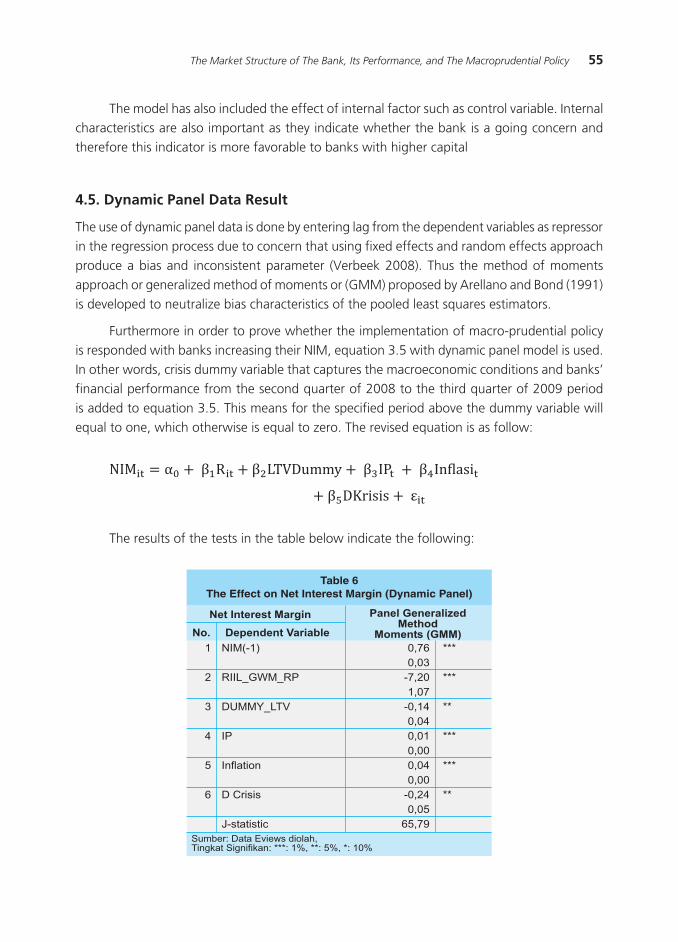
55The Market Structure of The Bank, Its Performance, and The Macroprudential Policy
The model has also included the effect of internal factor such as control variable. Internal characteristics are also important as they indicate whether the bank is a going concern and therefore this indicator is more favorable to banks with higher capital
4.5. Dynamic Panel Data Result
The use of dynamic panel data is done by entering lag from the dependent variables as repressor in the regression process due to concern that using fixed effects and random effects approach produce a bias and inconsistent parameter (Verbeek 2008). Thus the method of moments approach or generalized method of moments or (GMM) proposed by Arellano and Bond (1991) is developed to neutralize bias characteristics of the pooled least squares estimators.
Furthermore in order to prove whether the implementation of macro-prudential policy is responded with banks increasing their NIM, equation 3.5 with dynamic panel model is used. In other words, crisis dummy variable that captures the macroeconomic conditions and banks’ financial performance from the second quarter of 2008 to the third quarter of 2009 period is added to equation 3.5. This means for the specified period above the dummy variable will equal to one, which otherwise is equal to zero. The revised equation is as follow:
NIM R IP In�lasi
��������������������������������������������������������
�������������������
�
�
�
�
�
�
�����������������������
���������������� �������������������������
�����������
���������
��
���������
��������
�����������
���������������������������������������������������
�����
���
���
��
���
���
��
����������������������������������������������������������������������
The results of the tests in the table below indicate the following:
56 Bulletin of Monetary, Economics and Banking, Volume 18, Number 1, July 2015
Sargan test on the instrument yields p-value of 0.7706 that indicates that the null hypothesis is rejected and therefore the instrument used is proper. As shown in table above NIM (-1) has a coefficient 0.76, which is below 1 indicates that the influence of NIM with one quarter lag is not that significant. While the influence of the change of Reserve Requirement and LTV has a negative sign that corresponds to the expectation of the sign test. Similarly, negative coefficient on the crisis dummy variable, shows that NIM, a proxy of bank’s profitability, is affected during the specified period above. IP reflects the economy’s growth, in which its positive coefficient can be interpreted as there IP for each 1% increment on economic growth, there is 0.01% increase in NIM.
Macroeconomic factors in this study are represented by the level of inflation, the production Index and policy rate (BI Rate). As suggested by the sign of the policy rate coefficient, the variable is negative related to ROA of banks. One possible explanation is bank responds to increase interest rates, which translates to higher cost of funds for banks taking out loan. Policy rate however has a fairly low coefficient value. The small change of ROA for every 25 basis points change in policy rate could possibly be attributed to the returns that banks earn on their portfolio of Bank Indonesia Certificates (SBI) that is less risky compared to other productive assets like loans given to other banks.
The use of external variables in this research is intended to be a controlling variable that captures changes to the macro-economic cycle, which in theory influences banks’ behavior that affect their profitability. In theory, on the booming economic conditions or expansion stage of the economic cycle, banks tend to experience higher level of profitability as they are likely to increase the channeling of credit. On the other hand, during recession, banks tend to lower credit supply in line with falling credit demand by borrowers therefore banking profitability levels tend to decline.
V. CONCLUSION
As can be shown from Model 1 and 2 in the econonometric model, Reserve requirement ratio negatively affect the bank’s performance (ROA); a 1% increase in reserve requirement will reduce the ROA by 0.83%. Meaning that, the role of reserve requirement instruments as one of the macroprudential instrument is effective on stabilizing the financial bubble.
LTV policy also negatively affect the bank profitability. However for the banks with portfolio assets consisting marketable securities such as government bond or interbank call money, their strategy in anticipating change in the macro prudential policy is by changing the composition of deposits from expensive funding sources to less expensive ones such as saving and current deposit.
The market concentration (CR4) has a more significant effect on banks’ profitability as compared to market power (MS) This finding is supported by the p-value of market concentration,
57The Market Structure of The Bank, Its Performance, and The Macroprudential Policy
which proves CR4 to be significant at 5% significance level while MS is not. This finding is also supported by statistic of the four largest banks by asset and loan value and similar trend is also observed when the model is expanded to include eleven of the top banks.
In the Model 3 and 4, Production index and policy rate on Model 3 and 4 have significant effect on the banking profitability, which conform to interpretation on the negative coefficient. Increase of policy rate will result in increase of commercial banks’ interest rate and therefore cost of funding. However, under Model 1 and 2, it is observed that effect of policy rate on changes of the banks’ profitability is not significant as commercial banks responds to change in policy rate by increasing their interest rate that causes NIM to be unaffected.
LTV policy’s effect shows to be insignificant. From banks’ point of view, increase of reserve requirement is equivalent to extra tax burden that will be passed on to customers by increasing interest rate on loan or reducing of interest rate on deposits for customers. So the banking will respond to their clit by either increasing the rate loan or reducing deposit rate. This is done to maintain shareholder benefit, which is reflected by earning per share (EPS).
This paper provides some conclusions and policy recommendations; Firstly, the Central Banks need to understand the determinant of banks’ performance. Secondly, investigating the impact of macroprudential policies should take into account the market share aspect. Failure to understand the the interaction between macro-prudential instruments and market power might pose a risk to financial stability. These conclusions have policy implications on designing macroprudential instruments. For this reason, good coordination and joint research between the monetary and the fiscal authority is a necessity to provide financial stability.
Macro-Prudential Policy which consists of a compulsory reserve requirement (GWM) and LTV’s is aimed at achieving the objectives of macroeconomic stability and the stability of the financial system. In order to formulate effective policy and to promote healthy competition in the banking industry, it is necessary for regulator and policy maker to review the financial market structure. In oligopoly market, empirical test results have shown that the banking industry in Indonesia responded to increase in reserve requirement by raising the Net Interest Margin as to achieve targeted operating profits.
58 Bulletin of Monetary, Economics and Banking, Volume 18, Number 1, July 2015
REFERENCES
Arreguy et.all (IMF WP -13/167), Implementing Macroprudential, IMF.
Fabozzi, F. J., & T.B, T. 1986. State Taxes and Reserve Requirements as Major Determinants
of Yield Spreads Among Money Market Instruments. Journal of Financial and Quantitative Analysis , 21(4):427-36.
Grigorian dan Manole (2002), Determinant of Commercial Bank Performance in Transtion Economies: An Application of Data Envelopment Analysisis, The World bank, WP 2850.
Smirlock, M. 1985. ”Evidence of the (Non)-Relationship between Concentration and Probability
in Banking”, Journal of Money, Credit and Banking, vol.17, no.1,pp.69-83.
Verbeek, M. 2008. A Guide to Modern Econometrics, John Wiley & Sons, Ltd.
Xavier, Freixas and Jean Charles Rochet 2008, Microeconomic of Banking, 2nd Edition, The MIT Pres Cambridge, Massachusetts London, England.
59The Impact of Exchange Rate Misalignment on Safeguards Policy of ASEAN-5
THE IMPACT OF EXCHANGE RATE MISALIGNMENT ON SAFEGUARDS POLICY OF ASEAN-5
Dila VindayaniDedi Budiman Hakim
Alla Asmara1
The purposes of this study are to analyze the occurence of exchange rate misalignment and its effect
on non-tariff policy in ASEAN-5. We use Panel Dynamic OLS to estimate the equilibrium real exchange
rate, while for determining the opportunities of the Non-Tariff Measures (NTMs) such as safeguards
measures; we use Conditional Fixed-Effects Logistic Regression. The results shows that the magnitude of
exchange rate misalignment tends to be large when specific country has a domestic turmoil. In addition,
undervalued currrency of exporting country will increas the chances of safeguards measures enforcement
from partner countries.
Abstract
Keywords:Exchange rate misalignment, non-tarif measures (NTMs), safeguards, ASEAN, ACFTA.
JEL Classification: F13, O23, O24
1 Staff on Ministry of Trade and student on Economic Department, Institute Pertanian Bogor ([email protected]); adalah staf pengajar pada Departemen Ilmu Ekonomi, Fakultas Ekonomi dan Manajemen IPB ([email protected]); dan Alla Asmara adalah ([email protected]).

60 Bulletin of Monetary, Economics and Banking, Volume 18, Number 1, July 2015
I. INTRODUCTION
Trade is one of the important parts of real sectors that could drive economic activities. In this regards, international trade is belived to drive the creation of economic integration that could provide impact to one another and also to drive mobilitiy of goods and services. Therefore international trade is considered as the main focus of strategy to face liberalization era. The process of liberalization of trade is indicated by the establishment of General Agreement on
Tariffs and Trade (GATT) in 1947. Now its role has been replaced by World Trade Organization
(WTO). The goal of the establishment of the organization is to increase volume and value of world trade that is subsequently expected to drive higher economic growth and prosperity of the society all over the world.
Every country has been trying to strengthen their position on trade through their involvement in various bilateral, regional, and multilateral forum. Countries involved in international trade will theoretically perceive benefit as they will specialize in producing commodities efficiently. The agreement among countries of South East Asia through ASEAN is one of regional cooperations that attempts to intensify trades among intra- and extra-ASEAN countries. There are currently ten ASEAN countries which are Indoenesia, Singapore, Malaysia, Thailand, Philippines, Brunei Darussalam, Vietnam, Laos, Cambodia, and Myanmar. Each of them has unique economic condition where huge potential are available to be improved.
��������������������������������������������������������������������������������
������� ������
����
����
����
����
����
���������
�����������������
����
����� �����
������ ������ ������ ������
�������� ��� �������� ��� �������� ��� �������� ���
�������
���������
���������
���������
���������
�
������
������
������
������
�������
�������
���������
���������
���������
�
������
������
�����
�����
����������
����������
����������
����������
����������
�
������
������
�����
�����
����������
����������
����������
����������
����������
�
������
������
�����
�����
Table 1 expresses total export and import (expressed in million US) conducted by ASEAN and the world within the period of 2009 until 2013. The table also exhibits the growth from the previous period (in percentage). During the period, total export of ASEAN had been growing annually from US$ 813,787 million in 2009 to US$ 1,270,336 million in 2013. An impressive growth of export compared to the previous periods occurred in 2010 and 2011 by respectively 22% and 15%. Meanwhile export in 2012 and 2013 slightly grew by 1%. Total import of ASEAN has also increased within the last five years from US$ 726,591 million in 2009 to US$ 1,245,308 million. The rapid growth of import of ASEAN occurred in 2010 and 2011 by respectively 23%
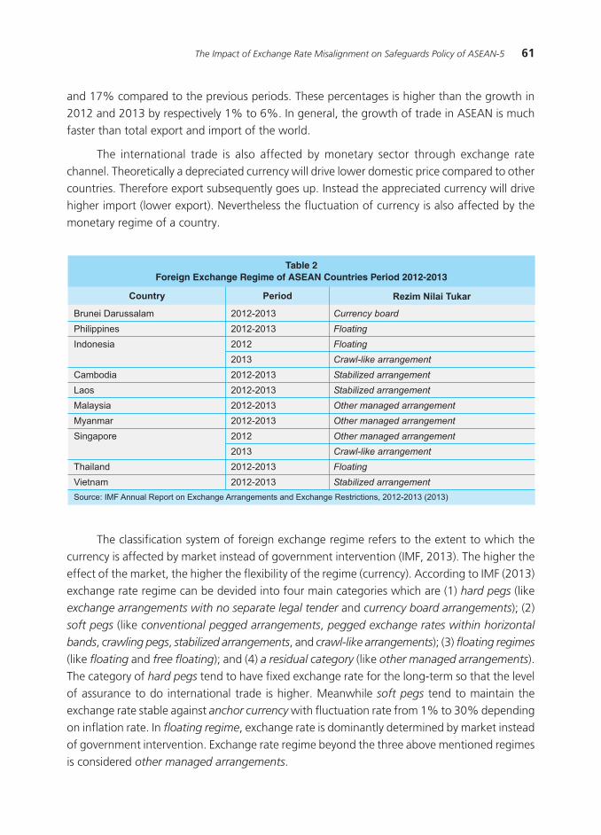
61The Impact of Exchange Rate Misalignment on Safeguards Policy of ASEAN-5
and 17% compared to the previous periods. These percentages is higher than the growth in 2012 and 2013 by respectively 1% to 6%. In general, the growth of trade in ASEAN is much faster than total export and import of the world.
The international trade is also affected by monetary sector through exchange rate channel. Theoretically a depreciated currency will drive lower domestic price compared to other countries. Therefore export subsequently goes up. Instead the appreciated currency will drive higher import (lower export). Nevertheless the fluctuation of currency is also affected by the monetary regime of a country.
The classification system of foreign exchange regime refers to the extent to which the currency is affected by market instead of government intervention (IMF, 2013). The higher the effect of the market, the higher the flexibility of the regime (currency). According to IMF (2013) exchange rate regime can be devided into four main categories which are (1) hard pegs (like exchange arrangements with no separate legal tender and currency board arrangements); (2) soft pegs (like conventional pegged arrangements, pegged exchange rates within horizontal
bands, crawling pegs, stabilized arrangements, and crawl-like arrangements); (3) floating regimes (like floating and free floating); and (4) a residual category (like other managed arrangements). The category of hard pegs tend to have fixed exchange rate for the long-term so that the level of assurance to do international trade is higher. Meanwhile soft pegs tend to maintain the exchange rate stable against anchor currency with fluctuation rate from 1% to 30% depending on inflation rate. In floating regime, exchange rate is dominantly determined by market instead of government intervention. Exchange rate regime beyond the three above mentioned regimes is considered other managed arrangements.
������������������������������������������������������������������
������� ������
�����������������
�����������
���������
��������
����
��������
�������
���������
��������
�������
���������
����������������������������������������������������������������������������������������������
������� �����������������������
���������
���������
����
����
���������
���������
���������
���������
����
����
���������
���������
��������������
��������
��������
����������������������
����������������������
����������������������
�������������������������
�������������������������
�������������������������
����������������������
��������
����������������������
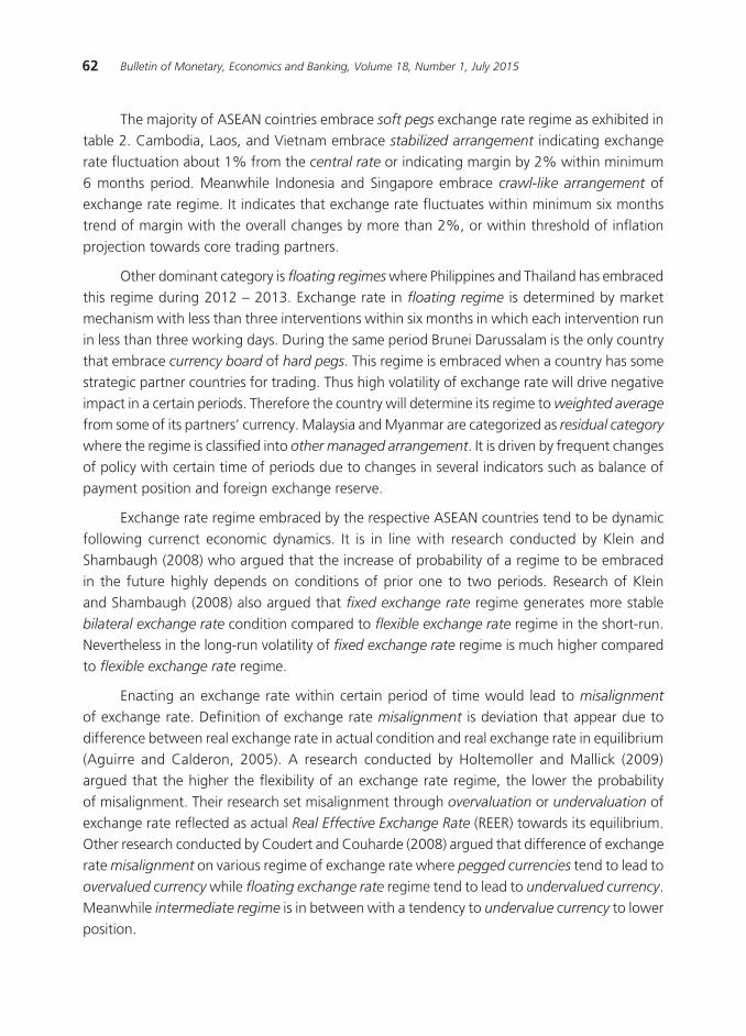
62 Bulletin of Monetary, Economics and Banking, Volume 18, Number 1, July 2015
The majority of ASEAN cointries embrace soft pegs exchange rate regime as exhibited in table 2. Cambodia, Laos, and Vietnam embrace stabilized arrangement indicating exchange rate fluctuation about 1% from the central rate or indicating margin by 2% within minimum 6 months period. Meanwhile Indonesia and Singapore embrace crawl-like arrangement of exchange rate regime. It indicates that exchange rate fluctuates within minimum six months trend of margin with the overall changes by more than 2%, or within threshold of inflation projection towards core trading partners.
Other dominant category is floating regimes where Philippines and Thailand has embraced this regime during 2012 – 2013. Exchange rate in floating regime is determined by market mechanism with less than three interventions within six months in which each intervention run in less than three working days. During the same period Brunei Darussalam is the only country that embrace currency board of hard pegs. This regime is embraced when a country has some strategic partner countries for trading. Thus high volatility of exchange rate will drive negative impact in a certain periods. Therefore the country will determine its regime to weighted average from some of its partners’ currency. Malaysia and Myanmar are categorized as residual category
where the regime is classified into other managed arrangement. It is driven by frequent changes of policy with certain time of periods due to changes in several indicators such as balance of payment position and foreign exchange reserve.
Exchange rate regime embraced by the respective ASEAN countries tend to be dynamic following currenct economic dynamics. It is in line with research conducted by Klein and Shambaugh (2008) who argued that the increase of probability of a regime to be embraced in the future highly depends on conditions of prior one to two periods. Research of Klein and Shambaugh (2008) also argued that fixed exchange rate regime generates more stable bilateral exchange rate condition compared to flexible exchange rate regime in the short-run. Nevertheless in the long-run volatility of fixed exchange rate regime is much higher compared to flexible exchange rate regime.
Enacting an exchange rate within certain period of time would lead to misalignment of exchange rate. Definition of exchange rate misalignment is deviation that appear due to difference between real exchange rate in actual condition and real exchange rate in equilibrium (Aguirre and Calderon, 2005). A research conducted by Holtemoller and Mallick (2009) argued that the higher the flexibility of an exchange rate regime, the lower the probability of misalignment. Their research set misalignment through overvaluation or undervaluation of exchange rate reflected as actual Real Effective Exchange Rate (REER) towards its equilibrium. Other research conducted by Coudert and Couharde (2008) argued that difference of exchange rate misalignment on various regime of exchange rate where pegged currencies tend to lead to overvalued currency while floating exchange rate regime tend to lead to undervalued currency. Meanwhile intermediate regime is in between with a tendency to undervalue currency to lower position.

63The Impact of Exchange Rate Misalignment on Safeguards Policy of ASEAN-5
Figure 1. Nominal Exchange Rate Movement in ASEAN, 2007-2012 (Domestic Currencies to USD, average)
Based on prior researches, misalignment condition can be considered from two aspects which are overvalued currency and undervalued currency. The theory of The Law of One Price (Krugman et al, 2012) expresses that overvalued currency occurred when exchange rate drive higher domestic price compared to global price. Meanwhile undervalued currency occurred when domestic price is lower than the global price, If a currency is overvalued then it will drive higher import as the price more competitive in the global market (Naseem et al, 2009). Undervalued currency will drive higher domestic production. Nevertheless protection policy overseas also increases (Irwin, 2011).
�����
�����
�����
�����
����
����� ���� ���� ���� ���� ����
��������� ������� ��������
������� �������
������������������������
��
��
��
��
��
��
����� ���� ���� ���� ���� ����
�������� ����������� ���������
�������� �����������������
The gap of monetary system and currency applied in each ASEAN countries lead to gap in exhange rate movement. It eventually affects the international trade. Figure 2 exhibits average-based nominal exchange rate movement during periods of 2007 to 2012 in ASEAN countries using monthly-based exchange rate calculation. Vietnamese Dong exchange rate movement has experienced depreciating trend within the last five years. Meanwhile Philippines Peso, Thailand Baht, and Laos Kip tend to appreciate during the same period. For Indonesia Rupiah, the movement of its exchange rate tend to fluctuate within the same period. Exchange rate appreciation drive the currency to overvalued, while depreciation lead the currency to be undervalued. The overvalued and undervalued conditions would lead to misalignment exchange rate in the long-run (Holtemöller and Mallick 2009).
The effect of misalignment effect due to overvalued or undervalued conditions will affect the orientation of international trade policy of a country. The policy of international trade tends to create barriers, which are tariff and non-tariff barriers. Tariff is tax or custom imposed commodities traded across borders, while non-tariff barriers are related to trade protection
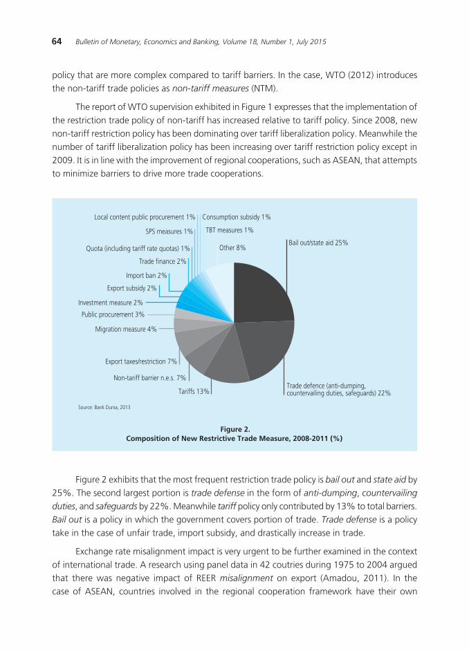
64 Bulletin of Monetary, Economics and Banking, Volume 18, Number 1, July 2015
policy that are more complex compared to tariff barriers. In the case, WTO (2012) introduces the non-tariff trade policies as non-tariff measures (NTM).
The report of WTO supervision exhibited in Figure 1 expresses that the implementation of the restriction trade policy of non-tariff has increased relative to tariff policy. Since 2008, new non-tariff restriction policy has been dominating over tariff liberalization policy. Meanwhile the number of tariff liberalization policy has been increasing over tariff restriction policy except in 2009. It is in line with the improvement of regional cooperations, such as ASEAN, that attempts to minimize barriers to drive more trade cooperations.
Figure 2. Composition of New Restrictive Trade Measure, 2008-2011 (%)
����������������������
���������������
������������������������������
�����������������������������������������������������������������������������
����������������������������
���������������������������
��������������������
���������������������
���������������������
�����������������
�������������
����������������
���������������������������������������
���������������
�����������������������������������
������������������������
Figure 2 exhibits that the most frequent restriction trade policy is bail out and state aid by 25%. The second largest portion is trade defense in the form of anti-dumping, countervailing
duties, and safeguards by 22%. Meanwhile tariff policy only contributed by 13% to total barriers. Bail out is a policy in which the government covers portion of trade. Trade defense is a policy take in the case of unfair trade, import subsidy, and drastically increase in trade.
Exchange rate misalignment impact is very urgent to be further examined in the context of international trade. A research using panel data in 42 coutries during 1975 to 2004 argued that there was negative impact of REER misalignment on export (Amadou, 2011). In the case of ASEAN, countries involved in the regional cooperation framework have their own
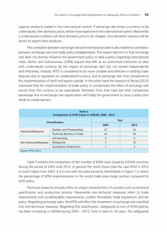
65The Impact of Exchange Rate Misalignment on Safeguards Policy of ASEAN-5
superior products traded in the international market. If exchange rate drives a currency to be undervalued, then domestic prices will be more expensive in the international market. Meanwhile a undervalued condition will drive domestic price to be cheaper, thus domestic industry will be driven to export their products.
The correlation between exchange rate and international rated is also related to correlation between exchange rate and trade policy misalignments. The reason behind it is that exchange rate does not directly influence the government policy to take a policy regarding international trade. Motto and Subramanian (2008) argued that IMF as an authorized institution to deal with undervalued currency (as the impact of exchange rate) has not served independently and effectively. Instead, WTO is considered to be more credible and effective in settling trade disputes due to regulation on undervalued currency, due to exchange rate, that complements the implementation of tariff and export subsidy. In the other hand the research of Nicita (2013) expressed that the implementation of trade policy to compensate the effect of exchange rate would drive the currency to be overvalued. Domestic firms that have lost their competitive advantage due to exchange rate appreciation will lobby the government to issue a policy that tends to create barriers.
����������������������������������������������������
������� ���������������
�����������������
������������������
���� ����
��
��
�
��
�
��
��
�
�
�
��������������������������
���������������������������
������������
����������
�������������������������
������������������
����������������������
Table 3 exhibits the comparison of the number of NTM cases issued by ASEAN countries during the period of 2003 until 2012. In general the result shows that the case NTM in 2012 in much higher than 2003. It is in line with the data issued by World Bank in Figure 1 in which the percentage of NTM implementation in the world trade place larger portion compared to tariff policy.
Technical measures actually refers to unique characteristics of a produc such as technical specification and production process. Meanwhile non-technical measures refers to trade requirements such as deliverables requirements, custom formalities, trade regulations, and tax policy. Regarding exchange rates, the NTM will effect the movement of exchange rate classified into non-technical measures. Regarding the classification, safeguards as one of NTM policies has been increasing in ASEAN during 2003 – 2012, from 3 cases to 10 cases. The safeguards

66 Bulletin of Monetary, Economics and Banking, Volume 18, Number 1, July 2015
action is implemented due to the increase in import of certain products that threats sustainability of domestic industry of importing countries. In this case, development of exchange rate would affect both export and import products (Thorstensen et al, 2011).
According to the previous description, it is seen that the correlation between exchange rate misalignment and trade in ASEAN countries needs to be further examined. It provides more space to researcher to deeply examine two important issues; first, how does exchange rate misalignment condition occur in ASEAN-5 currencies? Second, how does exchange rate misalignment affect safeguard policy in ASEAN-5 countries?
The next session of this paper discusses about the theory and empirical literature related to exchange rate misalignments. The third part provides data and methodology to analyze the data. The fourth session will discuss analyze estimation result, while conclusions and policy implication will be delivered in the fifth session of this research.
II. THEORY
2.1. Concept of Real Exchange Rate Equilibrium and Misalignment
The concept of real exchange rate equilibrium is an equilibrium condition if there is no tendency towards a change. Real exchange rate, as the most important mechanism of macroeconomic adjustment, will tend to change in the event of economic shocks. It will drive countinous change in currency rate therefore it will be difficult to be benchmark in determining equilibrium of real exchange rate. Therefore the concept of equilibrium will remain refer to economic condition without any shocks. In the other hand, the economy is assumed to have equilibrium in certain condition therefore the gap between actual and equilibrium has to be clearly visible. The equilibrium condition highly depends on current and expected future valuesn that are determined upon certain macroeconomic variables. It indicates that equilibrium is not static but will change over time similar to changes in variables value. Therefore, it is necessary to differentiate between short-run and long-run equilibrium. The difference between them is frequently called as exchange rate misalignment (Montiel, 2002).
The example is exhibited by the research of Montiel (2002) who assumed that real exchange rate is determined by the following reduced-from over time:
(1)
where X1 represents sustainable values of a set of real exogenous and policy variables, while X2 represents current values of a set of predetermined variables. The last variables are macroeconomic variables such as nominal wages, economy’s net international creditor position, dan capital stocks in traded and non-traded sectors which the value tends to be fixed over time, still, it gradually changes over time expressed as follow:
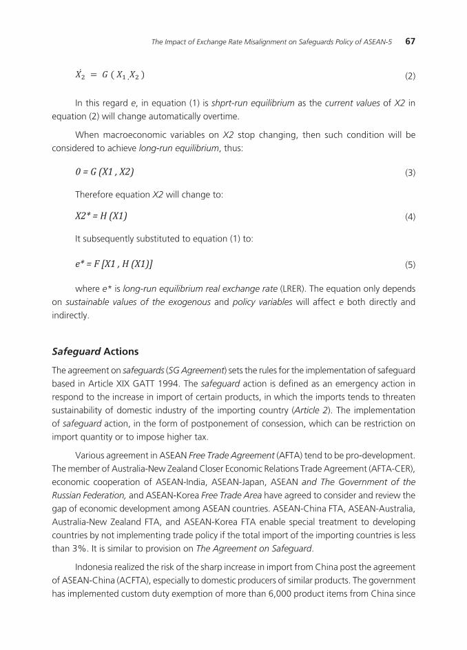
67The Impact of Exchange Rate Misalignment on Safeguards Policy of ASEAN-5
In this regard e, in equation (1) is shprt-run equilibrium as the current values of X2 in equation (2) will change automatically overtime.
When macroeconomic variables on X2 stop changing, then such condition will be considered to achieve long-run equilibrium, thus:
(2)
(3)
(4)
(5)
0 = G (X1 , X2)
X2* = H (X1)
e* = F [X1 , H (X1)]
Therefore equation X2 will change to:
It subsequently substituted to equation (1) to:
where e* is long-run equilibrium real exchange rate (LRER). The equation only depends on sustainable values of the exogenous and policy variables will affect e both directly and indirectly.
Safeguard Actions
The agreement on safeguards (SG Agreement) sets the rules for the implementation of safeguard based in Article XIX GATT 1994. The safeguard action is defined as an emergency action in respond to the increase in import of certain products, in which the imports tends to threaten sustainability of domestic industry of the importing country (Article 2). The implementation of safeguard action, in the form of postponement of consession, which can be restriction on import quantity or to impose higher tax.
Various agreement in ASEAN Free Trade Agreement (AFTA) tend to be pro-development. The member of Australia-New Zealand Closer Economic Relations Trade Agreement (AFTA-CER), economic cooperation of ASEAN-India, ASEAN-Japan, ASEAN and The Government of the
Russian Federation, and ASEAN-Korea Free Trade Area have agreed to consider and review the gap of economic development among ASEAN countries. ASEAN-China FTA, ASEAN-Australia, Australia-New Zealand FTA, and ASEAN-Korea FTA enable special treatment to developing countries by not implementing trade policy if the total import of the importing countries is less than 3%. It is similar to provision on The Agreement on Safeguard.
Indonesia realized the risk of the sharp increase in import from China post the agreement of ASEAN-China (ACFTA), especially to domestic producers of similar products. The government has implemented custom duty exemption of more than 6,000 product items from China since
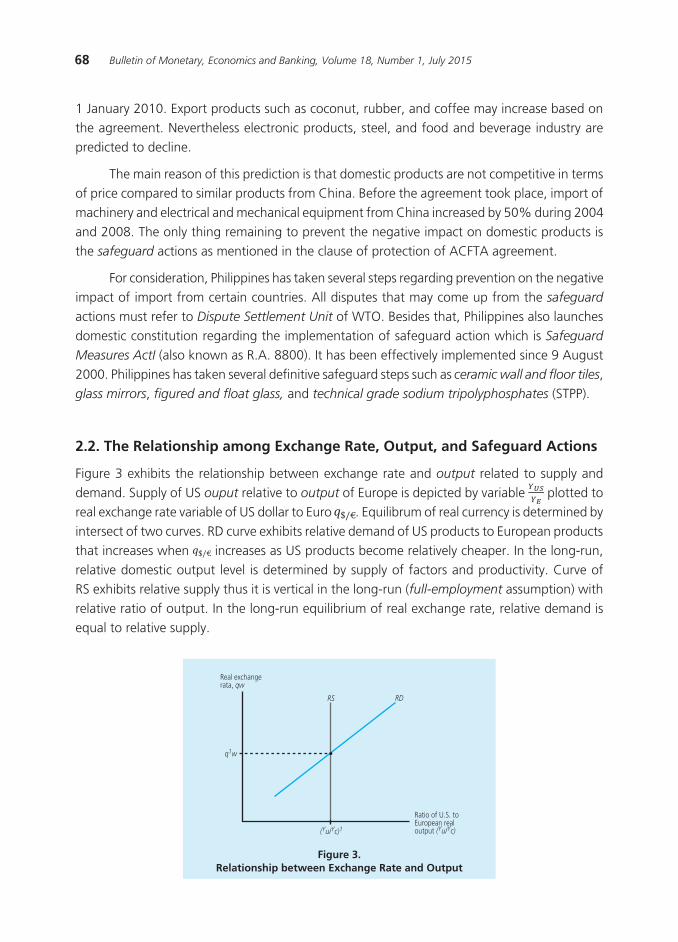
68 Bulletin of Monetary, Economics and Banking, Volume 18, Number 1, July 2015
1 January 2010. Export products such as coconut, rubber, and coffee may increase based on the agreement. Nevertheless electronic products, steel, and food and beverage industry are predicted to decline.
The main reason of this prediction is that domestic products are not competitive in terms of price compared to similar products from China. Before the agreement took place, import of machinery and electrical and mechanical equipment from China increased by 50% during 2004 and 2008. The only thing remaining to prevent the negative impact on domestic products is the safeguard actions as mentioned in the clause of protection of ACFTA agreement.
For consideration, Philippines has taken several steps regarding prevention on the negative impact of import from certain countries. All disputes that may come up from the safeguard actions must refer to Dispute Settlement Unit of WTO. Besides that, Philippines also launches domestic constitution regarding the implementation of safeguard action which is Safeguard
Measures ActI (also known as R.A. 8800). It has been effectively implemented since 9 August 2000. Philippines has taken several definitive safeguard steps such as ceramic wall and floor tiles, glass mirrors, figured and float glass, and technical grade sodium tripolyphosphates (STPP).
2.2. The Relationship among Exchange Rate, Output, and Safeguard Actions
Figure 3 exhibits the relationship between exchange rate and output related to supply and demand. Supply of US ouput relative to output of Europe is depicted by variable plotted to real exchange rate variable of US dollar to Euro . Equilibrum of real currency is determined by intersect of two curves. RD curve exhibits relative demand of US products to European products that increases when increases as US products become relatively cheaper. In the long-run, relative domestic output level is determined by supply of factors and productivity. Curve of RS exhibits relative supply thus it is vertical in the long-run (full-employment assumption) with relative ratio of output. In the long-run equilibrium of real exchange rate, relative demand is equal to relative supply.
�� ��
���������������������
���
��������
�������������������������������������������
����������������������������
Figure 3. Relationship between Exchange Rate and Output
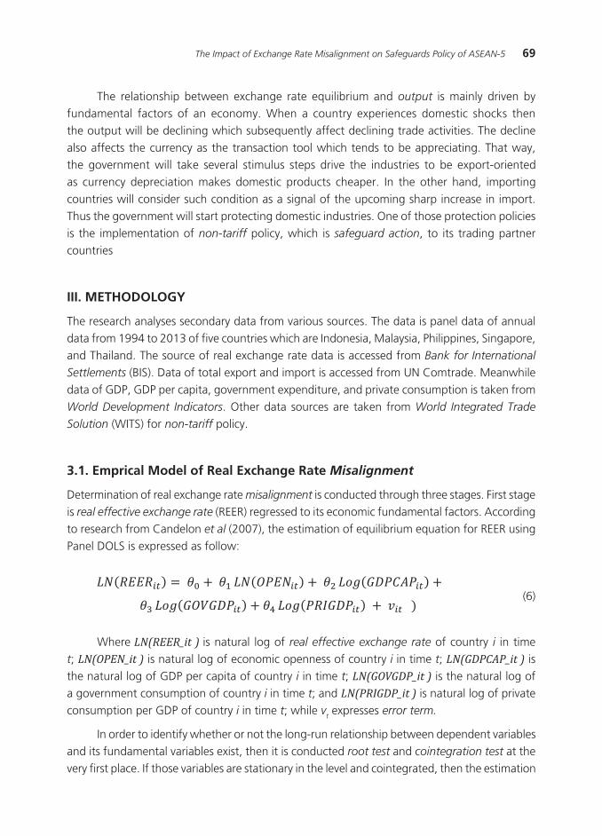
69The Impact of Exchange Rate Misalignment on Safeguards Policy of ASEAN-5
The relationship between exchange rate equilibrium and output is mainly driven by fundamental factors of an economy. When a country experiences domestic shocks then the output will be declining which subsequently affect declining trade activities. The decline also affects the currency as the transaction tool which tends to be appreciating. That way, the government will take several stimulus steps drive the industries to be export-oriented as currency depreciation makes domestic products cheaper. In the other hand, importing countries will consider such condition as a signal of the upcoming sharp increase in import. Thus the government will start protecting domestic industries. One of those protection policies is the implementation of non-tariff policy, which is safeguard action, to its trading partner countries
III. METHODOLOGY
The research analyses secondary data from various sources. The data is panel data of annual data from 1994 to 2013 of five countries which are Indonesia, Malaysia, Philippines, Singapore, and Thailand. The source of real exchange rate data is accessed from Bank for International
Settlements (BIS). Data of total export and import is accessed from UN Comtrade. Meanwhile data of GDP, GDP per capita, government expenditure, and private consumption is taken from World Development Indicators. Other data sources are taken from World Integrated Trade
Solution (WITS) for non-tariff policy.
3.1. Emprical Model of Real Exchange Rate Misalignment
Determination of real exchange rate misalignment is conducted through three stages. First stage is real effective exchange rate (REER) regressed to its economic fundamental factors. According to research from Candelon et al (2007), the estimation of equilibrium equation for REER using Panel DOLS is expressed as follow:
(6)
Where LN(REER_it ) is natural log of real effective exchange rate of country i in time t; LN(OPEN_it ) is natural log of economic openness of country i in time t; LN(GDPCAP_it ) is the natural log of GDP per capita of country i in time t; LN(GOVGDP_it ) is the natural log of a government consumption of country i in time t; and LN(PRIGDP_it ) is natural log of private consumption per GDP of country i in time t; while v
t expresses error term.
In order to identify whether or not the long-run relationship between dependent variables and its fundamental variables exist, then it is conducted root test and cointegration test at the very first place. If those variables are stationary in the level and cointegrated, then the estimation
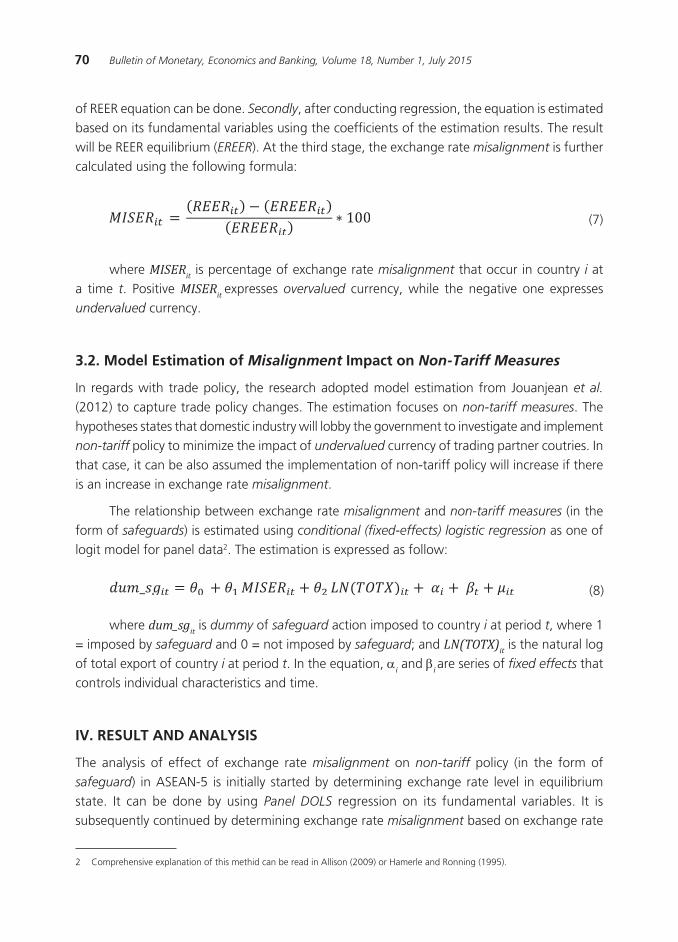
70 Bulletin of Monetary, Economics and Banking, Volume 18, Number 1, July 2015
of REER equation can be done. Secondly, after conducting regression, the equation is estimated based on its fundamental variables using the coefficients of the estimation results. The result will be REER equilibrium (EREER). At the third stage, the exchange rate misalignment is further calculated using the following formula:
(7)
where MISERit is percentage of exchange rate misalignment that occur in country i at a time t. Positive MISERit expresses overvalued currency, while the negative one expresses undervalued currency.
3.2. Model Estimation of Misalignment Impact on Non-Tariff Measures
In regards with trade policy, the research adopted model estimation from Jouanjean et al.
(2012) to capture trade policy changes. The estimation focuses on non-tariff measures. The hypotheses states that domestic industry will lobby the government to investigate and implement non-tariff policy to minimize the impact of undervalued currency of trading partner coutries. In that case, it can be also assumed the implementation of non-tariff policy will increase if there is an increase in exchange rate misalignment.
The relationship between exchange rate misalignment and non-tariff measures (in the form of safeguards) is estimated using conditional (fixed-effects) logistic regression as one of logit model for panel data2. The estimation is expressed as follow:
2 Comprehensive explanation of this methid can be read in Allison (2009) or Hamerle and Ronning (1995).
(8)
where dum_sgit is dummy of safeguard action imposed to country i at period t, where 1 = imposed by safeguard and 0 = not imposed by safeguard; and LN(TOTX)it is the natural log of total export of country i at period t. In the equation, ai and bi are series of fixed effects that controls individual characteristics and time.
IV. RESULT AND ANALYSIS
The analysis of effect of exchange rate misalignment on non-tariff policy (in the form of safeguard) in ASEAN-5 is initially started by determining exchange rate level in equilibrium state. It can be done by using Panel DOLS regression on its fundamental variables. It is subsequently continued by determining exchange rate misalignment based on exchange rate
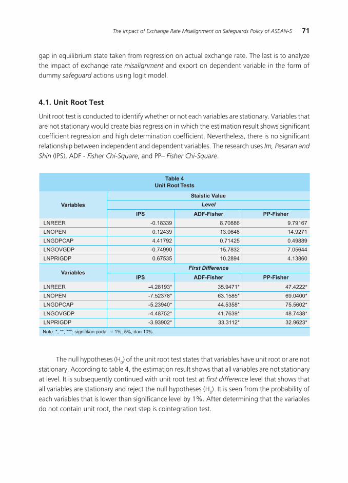
71The Impact of Exchange Rate Misalignment on Safeguards Policy of ASEAN-5
gap in equilibrium state taken from regression on actual exchange rate. The last is to analyze the impact of exchange rate misalignment and export on dependent variable in the form of dummy safeguard actions using logit model.
4.1. Unit Root Test
Unit root test is conducted to identify whether or not each variables are stationary. Variables that are not stationary would create bias regression in which the estimation result shows significant coefficient regression and high determination coefficient. Nevertheless, there is no significant relationship between independent and dependent variables. The research uses Im, Pesaran and
Shin (IPS), ADF - Fisher Chi-Square, and PP– Fisher Chi-Square.
����������������������
������������������������������������������������������
��������������
���������
���
������
������
��������
��������
��������
���������� ���������
�����
��������
�������
�������
��������
�������
�������
�������
�������
�������
�������
�������
�������
�������
�������
�������
������������ ���������� ���������
����������������
������
������
��������
��������
��������
���������
���������
���������
���������
���������
��������
��������
��������
��������
��������
��������
��������
��������
��������
��������
The null hypotheses (H0) of the unit root test states that variables have unit root or are not stationary. According to table 4, the estimation result shows that all variables are not stationary at level. It is subsequently continued with unit root test at first difference level that shows that all variables are stationary and reject the null hypotheses (H0). It is seen from the probability of each variables that is lower than significance level by 1%. After determining that the variables do not contain unit root, the next step is cointegration test.

72 Bulletin of Monetary, Economics and Banking, Volume 18, Number 1, July 2015
Cointegration Test
Cointegration test is run to identify whether or not there will be long-run equilibrium which is whether or not movement congruence and correlation stability between variables exist in this research. The assumption of null hypoytheses (H0) states that no cointegration, instead H1 states otherwise. Statistical criteria to reject H0 is the trace statistics > critical value or p-value which is lower than significance level.
��������������������������������
�������
�����������������
������������������
�������������������
������������������
�������������������
���
������� �������
�����������
����������
����������
����������
����������
����������
����������
����������
����������
����������
����������
�����������
����������
����������
����������
����������
�������
���
The research uses Pedroni dan Kao method to identify whether or not cointegration among variables. Cointegration test is run using three assumptions which are No deterministic
trend (Model 1), Deterministic intercept and trend (Model 2), and No deterministic intercept or trend (Model 3). According to result, it is found that all variables are cointegrated or reject H0. It indicates there is long-term relationship and equilibrium among variables.
4.2. Model Estimation of Real Exchange Rate Equilibrium
The equation of real exchange rate equilibrium is estimated by Panel DOLS using software EVIEWS
8. Fundamental variables to estimate real exchange rate equilibrium are degree of economic openness of a country, income per capita, government consumption per GDP, and private consumption per GDP. Degree of economic openness will increase the international integration this it would minimize trade barriers. Income per capita is an approach that is frequently used
�����������������������������������������������������
���������
������
��������
��������
��������
���������
����������� �����������
����������
�����������
����������
������������
��������
��������
���������
��������
���������

73The Impact of Exchange Rate Misalignment on Safeguards Policy of ASEAN-5
to measure productivity of a country. While government and private consumptions are variables frequently used to measure a demand of a country.
The estimation result shows that all fundamental variables have significant impact on effective real exchange rate where its probability level is less than significance level. Degree of economic openness has positive and significant impact on effective real exchange rate. It indicates that the higher the economic economic integration, the higher the appreciation of real exchange rate due to the increase in the use of domestic currency for transaction. Government consumption also has positive impact on effective real exchange rate. This condition expresses that government expenditure is allocated more on domestic expenditure so that real exchange rate is appreciated. In the other hand, income per capita and private consumption have negative impact on effective real exchange rate. It indicates the change in consumer goods when public gets earns higher income in which imported goods are more preferable so that demand on domestic currency declines and eventually leads to currency depreciation.
(9)
The R-squared of equation (9) is 0.964. It indicates that the estimation model of exchange rate equilibrium can be explained by variables of degree of economic openness, income per capital, government consumption, and private consumption by 96.4%, while the rest 3.6% is explained by other factors tha are not observed in this research. According to the coefficient of the estimation result, then equation (9) is recalculated with its fundamental variables to obtain the real exchange rate equilibrium.
4.3. Misalignment Condition of Exchange Rate in ASEAN-5 Countries
Misalignment condition of effective real exchange rate is obtained from gap percentage between the observed effective real exchange rate and the estimated real exchange rate equilibrium. The negative sign expresses an undervalued currency in which the effective real exchange rate is lower than the equilibrium level, thus the currency becomes depreciated. Meanwhile the positive sign indicates an overvalued currency in which the effective real exchange rate is higher than the equilibrium level so that the currency is appreciated.
The currency of Rupiah had far overvalued higher than the equilibrium level since 1998 as Indonesia still embraced fixed exchange rate regime. Nevertheless the effective real exchange rate condition then drastically changed to be lower than the equilibrium level from 1998 to 2002. Figure 4 exhibits Rupiah had been undervalued since monetary crisis 1998 due to domestic political instability. Domestic investment became not interested so that capital outflow occurred
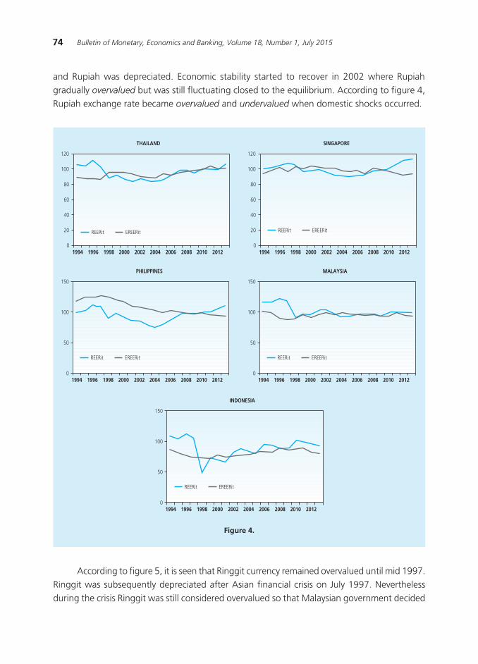
74 Bulletin of Monetary, Economics and Banking, Volume 18, Number 1, July 2015
and Rupiah was depreciated. Economic stability started to recover in 2002 where Rupiah gradually overvalued but was still fluctuating closed to the equilibrium. According to figure 4, Rupiah exchange rate became overvalued and undervalued when domestic shocks occurred.
Figure 4.
���
���
��
��
��
��
����� ���� ���� ���� ���� ���� ���� ���� ���� ����
��������
�������������
���
���
��
��
��
��
����� ���� ���� ���� ���� ���� ���� ���� ���� ����
���������
�������������
���� ���� ���� ���� ���� ���� ���� ���� ���� ����
�����������
�������������
���
���
��
����� ���� ���� ���� ���� ���� ���� ���� ���� ����
��������
�������������
���
���
��
�
���� ���� ���� ���� ���� ���� ���� ���� ���� ����
���������
�������������
���
���
��
�
According to figure 5, it is seen that Ringgit currency remained overvalued until mid 1997. Ringgit was subsequently depreciated after Asian financial crisis on July 1997. Nevertheless during the crisis Ringgit was still considered overvalued so that Malaysian government decided
75The Impact of Exchange Rate Misalignment on Safeguards Policy of ASEAN-5
to change its monetary policy regarding exchange rate regime from managed floating regimes
to pegged regimes in mid 1998. The policy was taken to minimize the negative impact from regional economic instability. In this case, the government of Malaysia was quite responsive to consider Ringgit as one determining factors in maintaining economic stability. According to figure 8, Ringgit was fluctuating in the next period closed to the equilibrium with small misalignment exchange rate.
Philippines experienced undervalued exchange rate with high misalignment exchange rate until 2007. It was the impact of trade liberalization that has been started in 1981 and run in three phases accompanied with import.
Liberalization Program (ILP) is a program that is intended to eliminate import barriers (Yap, 2008). The third phase is started in 1994 in which the tariff imposed was 3% for raw materials and capital goods that are not available domestically. Subsequently the government of Philippines committed to uniform tariff by 0 to 5% for most of the products in 2002. This situation drives Philippines to import capital goods so that Peso was depreciated. In 2008, Peso was gradually overvalued. This condition led to global financial crisis so that demand on dollar declined. Besides that, the capital inflow tends to be higher leading to demand on Peso.
Exchange rate of Singaporean dollar moved above the equilibrium condition in 1998. The situation shows that Singaporean economy tends to be stable eventhough Asian financial crisis occurred in 1997. Nevertheless Singaporean dollar became undervalued post financial crisis as the impact of declining regional economy. Singaporean dollar kept depreciating until global crisis 2008. According to figure 10, percentage of real exchange rate misalignment was relatively small until 2010. It was affected by monetary policy taken by the government of Singapore where currency rate setting referred to the main trading partner countries. In the other hand, Singaporean dollar has been overvalued since 2010. This condition is driven by the increase in capital inflow as the impact of positive prospect in Asia and depreciation of USD currency.
Baht exchange rate had been overvalued with relarively large percentage of misalignment since 1996. It was because Baht was pegged towards US dollar, thus when US dollar appreciates then Baht will appreciate as well, vise versa. It attracted many foreign investors to invest in Thailand. The appreciating Baht makes it least-competitive in doing export. Besides that, Baht exchange rate is also considered overvalued. As the consequences, investors started selling Baht in 1997 and made the currency undervalued. Economic condition in Thailand had started to recover since 2006 where Baht fluctuated closed to the equilibrium with low percentage of misalignment.
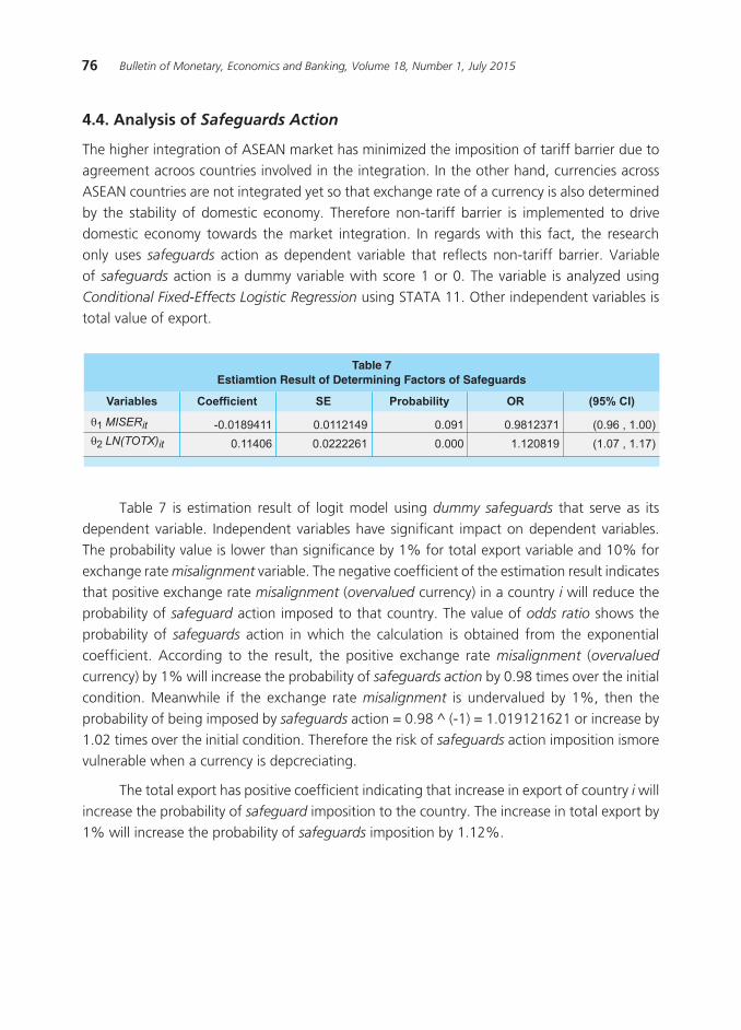
76 Bulletin of Monetary, Economics and Banking, Volume 18, Number 1, July 2015
4.4. Analysis of Safeguards Action
The higher integration of ASEAN market has minimized the imposition of tariff barrier due to agreement acroos countries involved in the integration. In the other hand, currencies across ASEAN countries are not integrated yet so that exchange rate of a currency is also determined by the stability of domestic economy. Therefore non-tariff barrier is implemented to drive domestic economy towards the market integration. In regards with this fact, the research only uses safeguards action as dependent variable that reflects non-tariff barrier. Variable of safeguards action is a dummy variable with score 1 or 0. The variable is analyzed using Conditional Fixed-Effects Logistic Regression using STATA 11. Other independent variables is total value of export.
�������������������������������������������������������������
���������
����������
�������������
����������� �� ����������� �� ��������
����������
�������
���������
���������
�����
�����
���������
��������
�������������
�������������
Table 7 is estimation result of logit model using dummy safeguards that serve as its dependent variable. Independent variables have significant impact on dependent variables. The probability value is lower than significance by 1% for total export variable and 10% for exchange rate misalignment variable. The negative coefficient of the estimation result indicates that positive exchange rate misalignment (overvalued currency) in a country i will reduce the probability of safeguard action imposed to that country. The value of odds ratio shows the probability of safeguards action in which the calculation is obtained from the exponential coefficient. According to the result, the positive exchange rate misalignment (overvalued currency) by 1% will increase the probability of safeguards action by 0.98 times over the initial condition. Meanwhile if the exchange rate misalignment is undervalued by 1%, then the probability of being imposed by safeguards action = 0.98 ^ (-1) = 1.019121621 or increase by 1.02 times over the initial condition. Therefore the risk of safeguards action imposition ismore vulnerable when a currency is depcreciating.
The total export has positive coefficient indicating that increase in export of country i will increase the probability of safeguard imposition to the country. The increase in total export by 1% will increase the probability of safeguards imposition by 1.12%.

77The Impact of Exchange Rate Misalignment on Safeguards Policy of ASEAN-5
V. CONCLUSION
The result of this research concludes that exchange rate misalignment percentage in ASEAN-5, both overvalued and undervalued; is likely large when domestic economy experiences shocks. A situation such as global crisis 2008 does not have large impact on the effective real exchange rate closed to its equilibrium. Besides that this research also revealed that the probability of an exporting country to be imposed by safeguard action from trading partner country is larger when the real exchange rate of the exporting country becomes undervalued (leading to depreciation of the exporting country’s currency).
Exchange rate misalignment that occurred in ASEAN countries has been minimized by each of the governments through reorientation of monetary policy to up dated to the current issues. In order to accelerate an attempt to overcome the negative impact, the ASEAN countries better work together regarding monetary policy. Safeguad action from ASEAN countries enables to minimize the impact of exchange rate instability. For instance Singapore that has weighted the exchange rate with its trading partner coutries so that the currency moves closed to the equilibrium. Therefore the economic integration in ASEAN Economic Community (AEC) scheme would be running smoothly.
The implementation of non-tariff policy is intended to protect domestic economy. It is predicted to increase along with the increase in the international trade agreement. In this research, non-tariff policy is limited to safeguards action due to lack of data. Therefore, it is necessary to conduct further research that deeply examines other non-tariff policies such as subsidy, SPS, and TBT.

78 Bulletin of Monetary, Economics and Banking, Volume 18, Number 1, July 2015
REFERENCES
Aaditya M, Arvind S. 2008. Currency undervaluation and sovereign wealth funds: a new role for the world trade organization. The World Bank Policy Research Working Paper. WP4668.
Alessandro N. 2013. Exchange rates, international trade and trade policies. UNCTAD. Study series no. 56.
Alvaro A, Cesar C. 2005. Real exchange rate misalignments and economic performance. Central
Bank of Chile Working Papers. No. 315.
Bertrand C, Clemens K, Katharina R, Tom VV. 2007. Long-run exchange rate determinants: evidence from eight new EU member states, 1993-2003. Elsevier Journal of Comparative
Economics. 35 (2007): 87-107.
[BIS] Bank for International Settlements. 2014. Real Effective Exchange Rates Data. http://www.bis.org/statistics/eer/. [terhubung berkala].
Diallo IA. 2011. The effects of real exchange rate misalignment and real exchange volatility on exports. MPRA Paper. No. 32387.
Douglas I. 2011. Trade policy and exchange rates. IMF/World Bank/WTO Workshop on
International Trade. The World Bank, 2 December 2011.
[IMF] International Monetary Fund. October 2013. Annual Report on Exchange Arrangements
and Exchange Restrictions 2013.
Hamerle, A., and G. Ronning. 1995. Panel analysis for qualitative variables. In Handbook of Statistical Modeling for the Social and Behavioral Sciences, ed. G. Arminger, C. C. Clogg, and M. E. Sobel, 401–451. New York: Plenum.
Josef TY. 2008. Policy Coherence Initiative on Growth, Investment and Employment: The Case of the Philippines (Policy Coherence and Critical Development Constraints in the Philippines). Paper prepared for the International Labour Organization (ILO).
Maria-Agnes J, Jean-Christophe M, Ben S. 2012. Reputation matters: spillover effects in the enforcement of US SPS measures. The World Bank: Policy Research Working Paper Series. WPS5935.
Michael WK, Jay CS. 2008. The dynamics of exchange rate regimes: fixes, floats, and flips. Elsevier Journal of International Economics. 75 (2008) 70–92.
N.A.M Naseem, Hui-Boon T, M.S Hamizah. 2008. Exchange rate misalignment, volatility and import flows in Malaysia. MPRA Paper. No. 41571.
79The Impact of Exchange Rate Misalignment on Safeguards Policy of ASEAN-5
Oliver H, Sushanta M. 2009. Does the choice of a currency regime explain real exchange rate misalignment?. The AIEFS session at ASSA Annual meeting 3-5 January, 2009.
Paul Allison, 2009, Fixed Effects Regression Models, Series: Quantitative Applications in the
Social Sciences, SAGE Publication.
Paul RK, Maurice O, Marc JM. 2012. International Economics : Theory & Policy. Boston (US): Pearson.
Peter JM. 2002. The long-run equilibrium real exchange rate: theory and measurement. Macroeconomic Management: Programs and Policies. Washington DC (US): IMF.
[UN COMTRADE] United Nations Comtrade. 2014. http://comtrade.un.org/data/. [terhubung berkala].
Vera T, Emerson M, Lucas F. 2011. Exchange rate misalignments and international trade policy: impacts on tariffs. Policy Dialogue: Redefining the Role of the Government in Tomorrow’s
International Trade at UNCTAD XIII Pre-Conference Event 26 – 27 March 2012.
[WB] World Bank. 2014. Official Exchange Rate (LCU per US$, period average) Data. http://data.worldbank.org/indicator/PA.NUS.FCRF. [terhubung berkala].
[WDI] World Development Indicators. 2014. http://data.worldbank.org/indicator. [terhubung berkala].
[WITS] World Integrated Trade Solution. 2014. Non-tariff Measures Data. http://wits.worldbank.org/. [terhubung berkala].
[WTO] World Trade Report. 2012. An Inventory of Non-Tariff Measures and Services
Measures.
[WTO] World Trade Organization. 2014. Total Merchandise Trade Data. http://stat.wto.org/StatisticalProgram/WSDBViewData.aspx?Language=E. [terhubung berkala].
[WTO] World Trade Organization. 2014. Non-Tariff Measures Data. http://i-tip.wto.org/goods/Forms/TableView.aspx. [terhubung berkala].

80 Bulletin of Monetary, Economics and Banking, Volume 18, Number 1, July 2015
This page intentionally left blank

81The Branch Expansion and The Performance of The Banks: The Case of Indonesia
THE BRANCH EXPANSION AND THE PERFORMANCE OF THE BANKS: THE CASE OF INDONESIA
Hery PrasetyoSony Sunaryo1
Opening new branches may help the banks to expand and is a priority for the banks to enlarge the
public inclusion. Indonesian banking industry is currently not efficient and still focus more on networking
the branches than improving the banking access to the public. This paper utilize the path analysis to see
the link betweeen the branch expansion and the performance of the banks. The analysis shows that
the increase of the number of branches and employees does not significantly influence the financial
performance of the banking industry from the period of 2011-2012. This prove that the inefficiency of
banking industry as one of the performance indicators of banking is not the main factor that be caused
by increasing the number of branches and employees.
Abstract
Keywords: Number of branches and employees, Financial performance of industrial banking, Path
Analysis.
JEL Classification: G21, L11
1 Authors ar lecturers at Magister Manajemen Teknologi, Institut Teknologi Sepuluh Nopember (Corresponding author: Hery Prasetyo, [email protected]).

82 Bulletin of Monetary, Economics and Banking, Volume 18, Number 1, July 2015
I. INTRODUCTION
Banking in Indonesia has a huge opportunity to expand extensively due to the huge market size, which has not been optimally managed. This regards is in accordance to the government programs to expand the banking service in the entire regions in Indonesia. One of the duties of the bank in Indonesia is to broaden the branch as wide as possible in order to get closer access to the customers and to escalate the banking service in the entire region in Indonesia. The branch opening has become the main priority in banking industry to be inclusive in the society.
Bank industry has such an essential role in economic growth. The economic growth history in Indonesia shows that the economics in this country moves forwards along with the banking industry. The economy in Indonesia is a bank-based economy, which is an economy that is depending on the existance of banks as the source of funding. Therefore, the efforts to strength a healthy, efficient and contributive bank system to the economy is the essential key of success in maintaining sustainability of the national economy development.
An economic crisis in 1997 was an incredibly substanstial lesson to the bank regulators in Indonesia regarding to the importance of the prudential regulation in managing banking system. Subsequent to the economy crisis in 1997 – 1988, there was a significant change of bank quantity in banking industry. There were 208 banks in 1998, which has decreased to 130 banks in 2006 and keep plunging to 121 in 2009 as it is shown in Table 1. The degradation of the bank quantity was caused by the repeal in bussiness permit and bank merger. The consolidation process through an effort to strengthen the capital and merger is expected to continue along with the program in Indonesia Banking Architecture, which was published in January 9th, 2004. Indonesia Bank Architecture (API) is a comprehensive framework basic system of banking in Indonesia and the one that provides guidance, form, and banking industry order in the period of five to ten years. The direction of regulation in the development of banking system in the future that has been defined by API was underlied by the vision to achievea heallthy, strong and efficient banking system to stabilise the banking system in order to boost the national economic growth.
����������������������������������������������
��������� ���� ���� ���� ���� ���� ���� ���� ���� ����
����������������� ��� ��� ��� ��� ��� ��� ��� ��� ��������
�������������������� ���� ���� �������� ������� ������� ������� ������� ������� �������
������������������������������������������������������������������������������������������������������������������������������������������������������������������������������������������������������
After the occurence of the global crisis in the financial sector in 2008, banking industry in Indonesia has not shown any responses towards this policy although Bank Indonesia has cut its rate to bank reference rate interest. It means that the bank as an intermediation institution
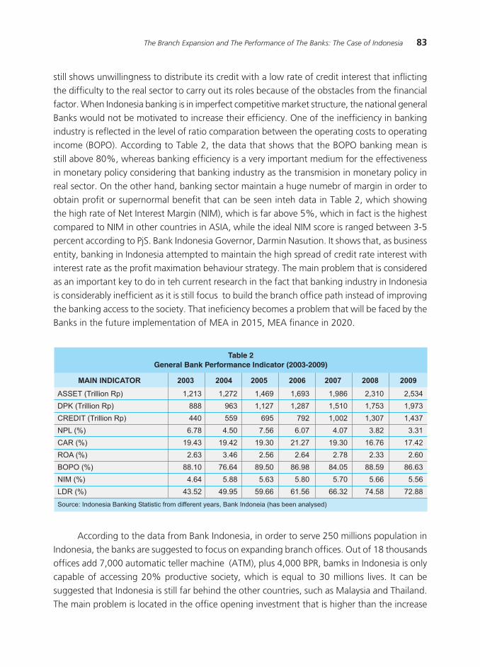
83The Branch Expansion and The Performance of The Banks: The Case of Indonesia
still shows unwillingness to distribute its credit with a low rate of credit interest that inflicting the difficulty to the real sector to carry out its roles because of the obstacles from the financial factor. When Indonesia banking is in imperfect competitive market structure, the national general Banks would not be motivated to increase their efficiency. One of the inefficiency in banking industry is reflected in the level of ratio comparation between the operating costs to operating income (BOPO). According to Table 2, the data that shows that the BOPO banking mean is still above 80%, whereas banking efficiency is a very important medium for the effectiveness in monetary policy considering that banking industry as the transmision in monetary policy in real sector. On the other hand, banking sector maintain a huge numebr of margin in order to obtain profit or supernormal benefit that can be seen inteh data in Table 2, which showing the high rate of Net Interest Margin (NIM), which is far above 5%, which in fact is the highest compared to NIM in other countries in ASIA, while the ideal NIM score is ranged between 3-5 percent according to PjS. Bank Indonesia Governor, Darmin Nasution. It shows that, as business entity, banking in Indonesia attempted to maintain the high spread of credit rate interest with interest rate as the profit maximation behaviour strategy. The main problem that is considered as an important key to do in teh current research in the fact that banking industry in Indonesia is considerably inefficient as it is still focus to build the branch office path instead of improving the banking access to the society. That ineficiency becomes a problem that will be faced by the Banks in the future implementation of MEA in 2015, MEA finance in 2020.
�����������������������������������������������������
�������������� ���� ���� ���� ���� ���� ���� ����
�������������������������������������������������������������������������������������������
������������������� ����� �������� �������� �������� �������� ��������� ��������
����������������� ���������������� ���������� ��������� �������� ������� ���������� �������
�������������������� ���������� ���������� ���������� ��������� ������� ���������� �������
������� ������������������������������ ���������� ���������� ��������� �������� ���������� ��������
������� ����������������������������� ��������� ��������� �������� ������� ���������� �������
������� ������������������������������ ���������� ��������� ��������� �������� ����������� ��������
�������� ���������������������������� ��������� �������� �������� ������� ��������� �������
������� ������������������������������� ���������� ��������� ��������� �������� ���������� ��������
������� ������������������������������ ��������� �������� ��������� ������� ��������� �������
According to the data from Bank Indonesia, in order to serve 250 millions population in Indonesia, the banks are suggested to focus on expanding branch offices. Out of 18 thousands offices add 7,000 automatic teller machine (ATM), plus 4,000 BPR, bamks in Indonesia is only capable of accessing 20% productive society, which is equal to 30 millions lives. It can be suggested that Indonesia is still far behind the other countries, such as Malaysia and Thailand. The main problem is located in the office opening investment that is higher than the increase
84 Bulletin of Monetary, Economics and Banking, Volume 18, Number 1, July 2015
of information technology access. Thailand, which only has 33 banks and 56 thousands branch is able to reach 73% of its community. As well as Malaysia with only 15 thousands branch offices, it could have banking scope until 66% of its productive ages population.
The interesting issue in Indonesia Banking is although BOPO has not been able to be efficient and is really eager to open lots of branch or network and increase the number of employee, but the profit that has been succesfully achieved by Indonesia Banking is considered as the highest compared to the other ASEAN countries.
Therefore, an analysis regarding the branch expansion and number of employee towards the banking performane in Indonesia, hence the link between the escalation of the number of branch and employee in banking efficiency (BOPO), credit distribution (loan to deposit ratio/LDR), problematic funding (non performance loan/NPL), the amount of net interest margin (NIM) in the rentability (return on asset/ROA) and (return on equity/ROE) banking industry in Indonesia to use Path Analysis as the objective in this research.
The result form the analysis is expected to provide the answer whether the effect of the branch opening and the increase of employee number in banking industry performance, and also explains whether the main cause of the banking inefficiency in Indonesia is due to the bank focus is in developingteh branch offices network and the increase of the number of employee at the same time, considering that the previous matters will be the potential problem in banking industry in implemeting MEA 2015 and MEA finance in 2020.
II. THEORY
The current study is investigating the role of branch opening strategy towards bank performance.; measured using numbers of performance indicators encompassed profitability, rentability, liquidity, risk management and managemenet productive activation skills. The first part of this chapter will discuss bank performance indicators that will be used. Furthermore, Theoretical model development will be applied in order to investigating the link between branch opening towards bank performance.
2.1. Banking Performance
Variabel return on asset (ROA) represent bank profitability, as return on equity (ROE) and return on capital (ROC). ROA is seen as the most approporate variable, which describing bank industry profitability (Berger, 2009). The ROA ratio formula is Laba excluded tax within the last12 months/Mean activa during the similar period (accordign to SE BI No. 30/2/UPB 30 April 1997) with percentage (%).
85The Branch Expansion and The Performance of The Banks: The Case of Indonesia
The second bank performance parameter is rentability ratio (earnings). The success of a Bank is based on the quantitative appraisal towards bank rentability can be measured by using operational cost ratio towards operational income or BOPO (Kuncoro & Suhardjono, 2002). Bank Indonesia defines the best ratio for BOPO ratio is below 90%, because if BOPO ratio exceeded 90% reaching to 100%, then it means that the bank runs the its operation inefficiently. In 2013 BI published BOPO ratio policy based on Bank Umum kelompok usaha (BUKU). Maximum BOPO BUKU I is 85%, BUKU II is approximately 78%-80%, BUKU III 70%-75% and BUKU IV 65%-60%. Dendawijaya (2003) stated that operational cost ratio that is used to measure the level of efficiency and the bank capability in executing its operational activities. Ratio BOPO is often called as efficiency ratio that is used to examine a bank management capability to manage the operational cost towards operationl income. The smaller the ratio the more efficient the outcome of the operational cost from the bank (Almilia & Herdiningtyas, 2005).
BOPO is calculated from the ratio between operational cost towards operational income (SE BI No 6/73/INTERN DPNP 24 December 2004). The operational cost is summed based on the the total sum of interest expense and the total of the other operational cost. Operational income is the sum of the total interest income and the other operational incomes.
Liquidity is the third bank performance indicator. In this regards, Loan to Deposit Ratio (LDR) can be used to evaluate a bank liquidity by dividing the credit amount with the funding amount (Almilia & Herdiningtyas, 2005). Loan to Deposit Ratio (LDR) represent a bank capability in providing funding to its debitur from the “Modal” that is owned by the bank or funding that can be collected from the community/society. Dendawijaya, Lukman (2003), Loan to Deposit Ratio (LDR) states to what extent a bank capability in repaying the funding withdrawal by the deposan, by realying on the credit that has been given as its liquidity sources. The higher teh LDR shows thte indication, the lower the bank’s liquidity capability. This problem occurs becasue the amount of funding that is needed to fund the credit grows bigger.
The capability to manage the risk is also an important indicator for bank performance. Spesifically according to Bank Indonesia policy No. 5, year 2003, risk is a an event that is potentially harmful and damaging. Hence, due to the significant development of Bank Indonesia policy circumstances in internal and external banking, one of the risk in banking is the credit risk, which is defined as: an emerged risk as the cost of the counterparty failure to fulfil its obligation. Credit risk is a risk that is caused because the bank dispense its funding in a form or loan to the society. Accordingly, there is a possibility that the debitur would not fulfil their obligation to the bank such as loan principal payments, interest payments, etc. Teh failur of those obligation fulfiment by the bank customer that can bring the harm to the bank because the previous unaccepted payment has been predicted.
86 Bulletin of Monetary, Economics and Banking, Volume 18, Number 1, July 2015
Accordingly, in order to run a bussiness it is important to anticipate the possible risks that is likely to emerge. The management needs to minimise the risk that is likely to occur in managing/organising production factors, source funding, and investment risl ratio, credit risk ratio, capital risk ratio, deposit risk ratio and interest risk ratio. The measurement is essentially connected to return measurement because bank face the possible risk that might occur in order to get the return. Credit management is an important thing in a company, which is operating in providing credit as the bigger the credit the bigger the risk. Therefore, should a bank is in condition of high NLP then it will enlarge both the cost of backup productive activa or any other cost that result in emerging the loss for the bank. NPL is calculated as ratio from the amount of the problematic credit towards total credit (Kasmir, 2006).
The capability of bank management constitutes important indicators that has to be considered in this paper. Net Interest Margin form the ratio that represent the capability of the bank management in organising its productive activa in order to produce the net income interest. The bigger the ratio cause an increse in income interest from the productive activa which minimise the problem that is likely to occur in the bank (Almilia & Herdiningtyas, 2005)
Rose P (2002) explains that Net Interest Margin indicates how well the capability of the bank management and employee in obtaining the income (particularly from credit and invesment) compared to the cost (that basically comes from the deposite interest). Koch and Scott (2000) emphasis the importance Net Interest Margin to evaluate bank competence in managing risk of rate interest. The change in rate interest will also alter the interest income and the cost of bank interest. For instance, when the rate interest increse, both the income interest and the cost interest will also increase because some assets and the bank obligation will be valued in a higher level.
Net Interest Margin (NIM) is calculated as a ratio from the net interest income towards activa productive. The net interest income is obtained from the difference of interest income and interest expense. Activa productive constitutes an bank funding invesment in IDR or in foreign exchange in credit, important documents, the funding placement among banks, equalisation, including commitment and contingency in account administration transaction.

87The Branch Expansion and The Performance of The Banks: The Case of Indonesia
Picture 1. Path diagram of the Research Theoretical Model
����������������������
�����������������������
��������
��������
���������
��������
��������
��������
�
�
�
�
��
��
��
��
��
��
��
��
�
��������������
���
������������
���
���
�
The conceptual framework above constitutes the complete structural model that can be broken down into numbers of sub-structural mode below:
Sub Structure 1: (Y1) = ρ1X1 + ρ5X2 + e1
2.2. Development of the Theoretical Model
The theoretical model that will be developed is presented in the path diagram below:
Picture 2.Substructure Model Diagram 1
����������������������
�����������������������
���������
����
��
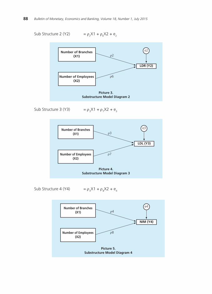
88 Bulletin of Monetary, Economics and Banking, Volume 18, Number 1, July 2015
Picture 5.Substructure Model Diagram 4
Picture 3.Substructure Model Diagram 2
Picture 4.Substructure Model Diagram 3
����������������������
�����������������������
��������
����
��
Sub Structure 3 (Y3) = ρ3X1 + ρ7X2 + e3
Sub Structure 2 (Y2) = ρ2X1 + ρ6X2 + e2
Sub Structure 4 (Y4) = ρ4X1 + ρ8X2 + e4

89The Branch Expansion and The Performance of The Banks: The Case of Indonesia
Picture 6.Substructure Model Diagram 5
Sub Structure 5 (Z1) = ρ9X1 + ρ10X2 + ρ11Y1 + ρ12Y2 + ρ13Y3 + ρ14Y4 + e5
Sub Structure 6 (Z2) = ρ15X1 + ρ16X2 + ρ17Y1 + ρ18Y2 + ρ19Y3 + ρ20Y4 + e6
Picture 7.Substructure Model Diagram 6
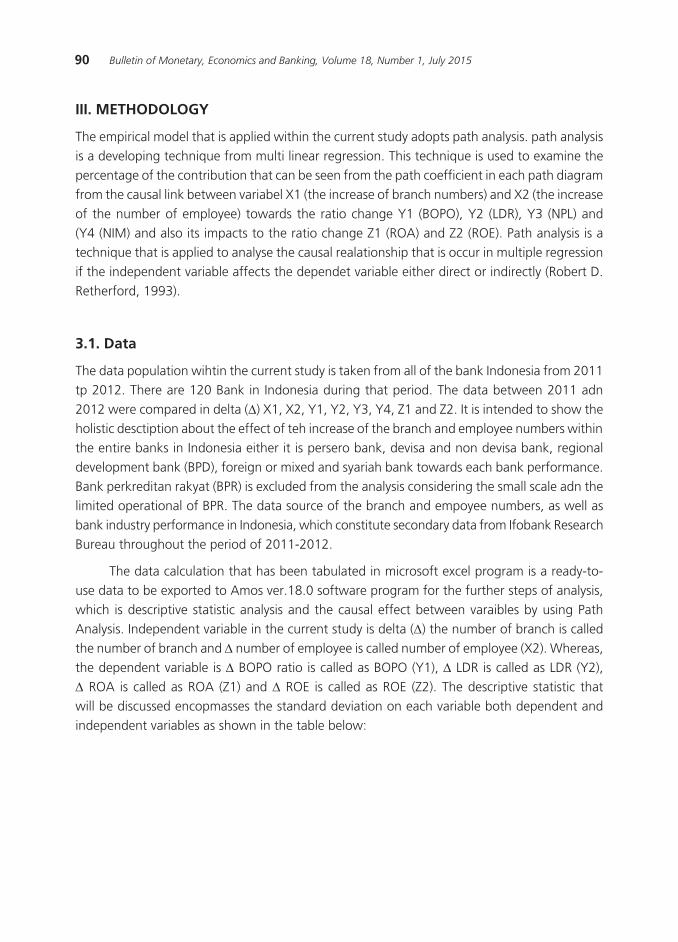
90 Bulletin of Monetary, Economics and Banking, Volume 18, Number 1, July 2015
III. METHODOLOGY
The empirical model that is applied within the current study adopts path analysis. path analysis is a developing technique from multi linear regression. This technique is used to examine the percentage of the contribution that can be seen from the path coefficient in each path diagram from the causal link between variabel X1 (the increase of branch numbers) and X2 (the increase of the number of employee) towards the ratio change Y1 (BOPO), Y2 (LDR), Y3 (NPL) and (Y4 (NIM) and also its impacts to the ratio change Z1 (ROA) and Z2 (ROE). Path analysis is a technique that is applied to analyse the causal realationship that is occur in multiple regression if the independent variable affects the dependet variable either direct or indirectly (Robert D. Retherford, 1993).
3.1. Data
The data population wihtin the current study is taken from all of the bank Indonesia from 2011 tp 2012. There are 120 Bank in Indonesia during that period. The data between 2011 adn 2012 were compared in delta (∆) X1, X2, Y1, Y2, Y3, Y4, Z1 and Z2. It is intended to show the holistic desctiption about the effect of teh increase of the branch and employee numbers within the entire banks in Indonesia either it is persero bank, devisa and non devisa bank, regional development bank (BPD), foreign or mixed and syariah bank towards each bank performance. Bank perkreditan rakyat (BPR) is excluded from the analysis considering the small scale adn the limited operational of BPR. The data source of the branch and empoyee numbers, as well as bank industry performance in Indonesia, which constitute secondary data from Ifobank Research Bureau throughout the period of 2011-2012.
The data calculation that has been tabulated in microsoft excel program is a ready-to-use data to be exported to Amos ver.18.0 software program for the further steps of analysis, which is descriptive statistic analysis and the causal effect between varaibles by using Path Analysis. Independent variable in the current study is delta (∆) the number of branch is called the number of branch and ∆ number of employee is called number of employee (X2). Whereas, the dependent variable is ∆ BOPO ratio is called as BOPO (Y1), ∆ LDR is called as LDR (Y2), ∆ ROA is called as ROA (Z1) and ∆ ROE is called as ROE (Z2). The descriptive statistic that will be discussed encopmasses the standard deviation on each variable both dependent and independent variables as shown in the table below:

91The Branch Expansion and The Performance of The Banks: The Case of Indonesia
����������������������������������������������������
�������� ������ ��� ��� ���� ������������
����������������������������������������
�����������������
�������������������
����
���
���
���
���
���
���� � ���� ������ ������
���� � ���� ������ ������
��������� ��� ��� ����� �����
���� � ����� ������� �������
���� � ����� ������� �������
��������� ���� ���� ������ ������
���� ����� ������ ����� �����
���� ����� ������ ����� �����
��������� ������ ����� ����� ����
���� ����� ������ ����� �����
���� ����� ������ ����� �����
��������� ����� ����� ���� �����
���� � ���� ���� ����
���� � ���� ���� ����
��������� ���� ���� ����� ����
���� ���� ����� ���� ����
���� ���� ����� ���� ����
��������� ����� ���� ����� ����
���� ����� ���� ���� ����
���� ���� ���� ���� ����
��������� ����� ���� ����� ����
���� ������ ����� ����� �����
���� ����� ����� ����� �����
��������� ������ ����� ���� ����
3.2. Data Analysis Technique
The empirical model that will be developed will be analysed by using Path Analyis. The use of Path analysis allows the current study to analyse a more complex empirical model and constitute an elaboration of multiple regression. Path analysis model is applied in analysing the pattern of the link between variables within the current study in order to discover both the direct and indirect effects of independent variables on the dependent variables. Independent variables in the current study are ∆ the number of branch (X1) and ∆ numbe rof employee (X2). Whereas, the dependent variables are the ratios of ∆ BOPO (Y1), ∆ LDR (Y2), ∆ NPL (Y3), ∆ NIM (Y4), ∆ ROA (Z1) and ∆ ROE (Z2). Path analysis is an elaboration of multiple regression, hence the prerequisites and the examinations in multiple regressions is also applied in path analysis.
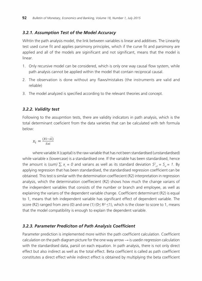
92 Bulletin of Monetary, Economics and Banking, Volume 18, Number 1, July 2015
3.2.1. Assumption Test of the Model Accuracy
Wihtin the path analysis model, the link between variables is linear and additives. The Linearity test used curve fit and applies parsimony principles, which if the curve fit and parsimony are applied and all of the models are siginificant and not significant, means that the model is linear.
1. Only recursive model can be considered, which is only one way causal flow system, while path analysis cannot be applied within the model that contain reciprocal causal.
2. The observation is done without any flaws/mistakes (the instruments are valid and reliable)
3. The model analyzed is specified according to the relevant theories and concept.
3.2.2. Validity test
Following to the assupmtion tests, there are validity indicators in path analysis, which is the total determinant coeficient from the data varieties that can be calculated with teh formula below:
where variable X (capital) is the raw variable that has not been standardised (unstandardised) while variable x (lowercase) is a standardised one. If the variable has been standardised, hence the amount is (sum) ∑ x
i = 0 and varians as well as its standard deviation S2
x1 = S
xi = 1. By
applying regression that has been standardised, the standardised regression coefficient can be obtained. This test is similar with the determination coeffiecient (R2) interpretation in regression analysis, which the determination coeffiecient (R2) shows how much the change varians of the independent variables that consists of the number or branch and employee, as well as explaining the varians of the dependent variable change. Coefficient determinant (R2) is equal to 1, means that teh independent variable has significant effect of dependent variable. The score (R2) ranged from zero (0) and one (1) (0≤ R² ≤1), which is the closer to score to 1, means that the model compatibility is enough to explain the dependent variable.
3.2.3. Parameter Prediciton of Path Analysis Coefficient
Parameter prediction is implemented more within the path coefficient calculation. Coefficient calculation on the path diagram picture for the one way arrow → is usedin regression calculation with the standardised data, parsiil on each equation. In path analysis, there is not only direct effect but also indirect as well as the total effect. Beta coefficient is called as path coefficient constitutes a direct effect while indirect effect is obtained by multiplying the beta coefficient
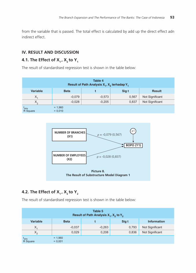
93The Branch Expansion and The Performance of The Banks: The Case of Indonesia
from the variable that is passed. The total effect is calculated by add up the direct effect adn indirect effect.
IV. RESULT AND DISCUSSION
4.1. The Effect of X1 , X2 to Y1
The result of standardised regression test is shown in the table below:
�������������������������������������������������
�������� ���� � ����� ������
�� ������ ������ ����� ���������������
��
������ ������ ����� ���������������
����� � ������������� � �����
Picture 8.The Result of Substructure Model Diagram 1
4.2. The Effect of X1 , X2 to Y2
The result of standardised regression test is shown in the table below:
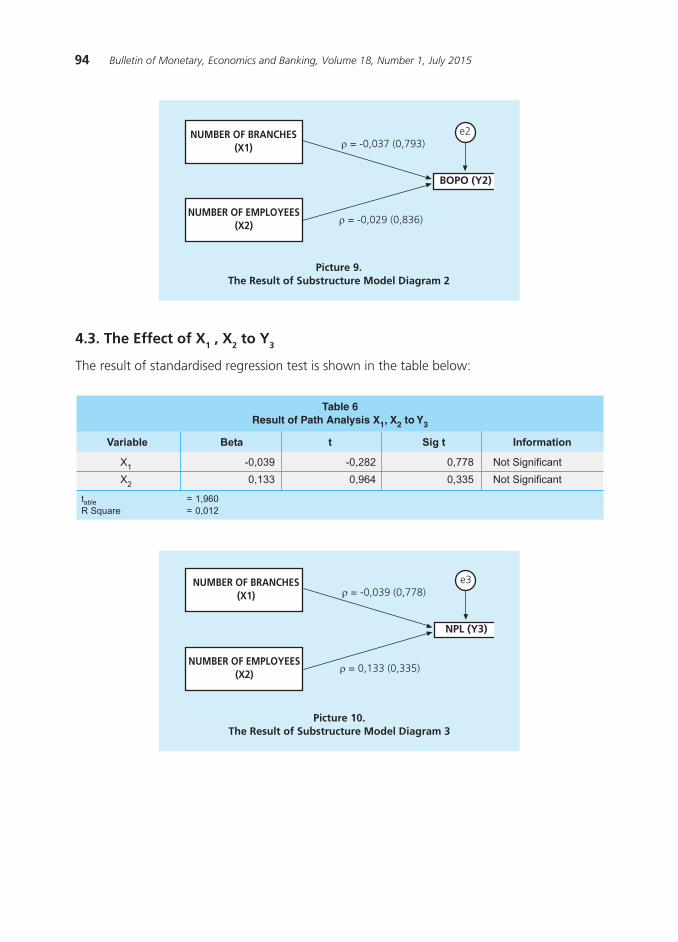
94 Bulletin of Monetary, Economics and Banking, Volume 18, Number 1, July 2015
Picture 10.The Result of Substructure Model Diagram 3
Picture 9.The Result of Substructure Model Diagram 2
4.3. The Effect of X1 , X2 to Y3
The result of standardised regression test is shown in the table below:
�������������������������������������������
�������� ���� � ����� �����������
�� ������ ������ ����� ���������������
�� ����� ����� ����� ���������������
����� � ������������� � �����
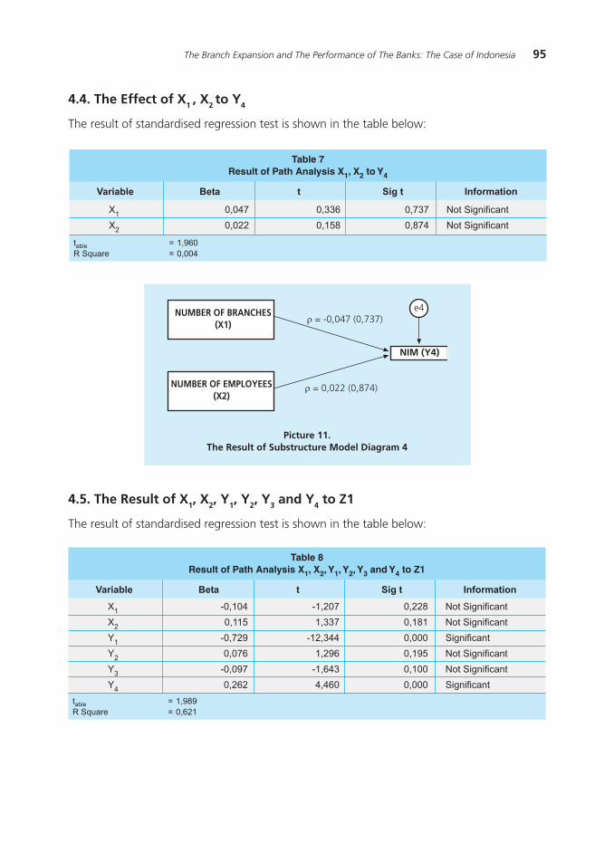
95The Branch Expansion and The Performance of The Banks: The Case of Indonesia
4.4. The Effect of X1 , X2 to Y4
The result of standardised regression test is shown in the table below:
�������������������������������������������
�������� ���� � ����� �����������
�� ����� ����� ����� ���������������
�� ����� ����� ����� ���������������
����� � ������������� � �����
4.5. The Result of X1, X2, Y1, Y2, Y3 and Y4 to Z1
The result of standardised regression test is shown in the table below:
Picture 11.The Result of Substructure Model Diagram 4

96 Bulletin of Monetary, Economics and Banking, Volume 18, Number 1, July 2015
4.6. The Effect of X1, X2, Y1, Y2, Y3 and Y4 to Z2
The result of standardised regression test is shown in the table below:
Picture 12.The Result of Substructure Model Diagram 5

97The Branch Expansion and The Performance of The Banks: The Case of Indonesia
4.7. Fit Model Analysis
According to fit model test, it is discovered that the current research model is fit because it meets the test index based on the required rule of thumb. It means that, the model can be empirically tested and applied within the current study. The result of the test is summarised within the table below:
Picture 13.The Result of Substructure Model Diagram 6
������������������������������������������������
��������������������� ������������ ������ �����������
���������� ����������� ������ ������������������
����������� ������� ����� ������������������
������� ������� ����� ������������������
����� ������� ����� ������������������
��� ������� ����� ���������
���� ������� ����� ������������������
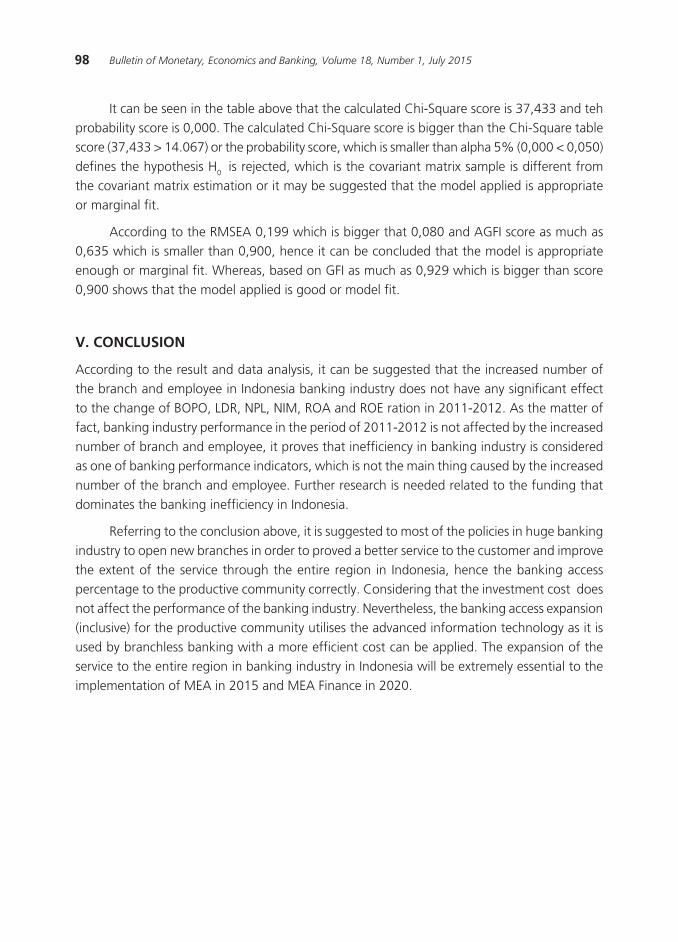
98 Bulletin of Monetary, Economics and Banking, Volume 18, Number 1, July 2015
It can be seen in the table above that the calculated Chi-Square score is 37,433 and teh probability score is 0,000. The calculated Chi-Square score is bigger than the Chi-Square table score (37,433 > 14.067) or the probability score, which is smaller than alpha 5% (0,000 < 0,050) defines the hypothesis H0 is rejected, which is the covariant matrix sample is different from the covariant matrix estimation or it may be suggested that the model applied is appropriate or marginal fit.
According to the RMSEA 0,199 which is bigger that 0,080 and AGFI score as much as 0,635 which is smaller than 0,900, hence it can be concluded that the model is appropriate enough or marginal fit. Whereas, based on GFI as much as 0,929 which is bigger than score 0,900 shows that the model applied is good or model fit.
V. CONCLUSION
According to the result and data analysis, it can be suggested that the increased number of the branch and employee in Indonesia banking industry does not have any significant effect to the change of BOPO, LDR, NPL, NIM, ROA and ROE ration in 2011-2012. As the matter of fact, banking industry performance in the period of 2011-2012 is not affected by the increased number of branch and employee, it proves that inefficiency in banking industry is considered as one of banking performance indicators, which is not the main thing caused by the increased number of the branch and employee. Further research is needed related to the funding that dominates the banking inefficiency in Indonesia.
Referring to the conclusion above, it is suggested to most of the policies in huge banking industry to open new branches in order to proved a better service to the customer and improve the extent of the service through the entire region in Indonesia, hence the banking access percentage to the productive community correctly. Considering that the investment cost does not affect the performance of the banking industry. Nevertheless, the banking access expansion (inclusive) for the productive community utilises the advanced information technology as it is used by branchless banking with a more efficient cost can be applied. The expansion of the service to the entire region in banking industry in Indonesia will be extremely essential to the implementation of MEA in 2015 and MEA Finance in 2020.
99The Branch Expansion and The Performance of The Banks: The Case of Indonesia
REFERENCES
Amalia, Fitri dan Nasution, Mustafa Edwin. 2007. Perbandingan Profitabilitas Industri Perbankan
Syariah dan Industri Perbankan Konvensional menggunakan Metode Struktur KInerja dan
Perilaku. Jurnal Ekonomi dan Pembangunan Indonesia. Vol VII, no.02, 2007.
Almilia, Luciana Spica dan Herdiningtyas, Winny. 2005. Analisis Rasio CAMEL terhadap Prediksi Kondisi Bermasalah pada Lembaga Perbankan Periode 2000-2002. Jurnal Akuntansi dan
Keuangan, Vol, 7, No, 2, Nopember, hal,1-27, 2005.
Bank Indonesia. 2008. Statistik Perbankan Indonesia, Statistik Perbankan Indonesia, Volume 6, No 10, September 2008, Available online at http://www.bi.go.id/web/id.
Bikker, JA. 2002. Competition, Concentration, and Their Relationship: An Empirical at The Banking Industry, Journal of Banking and Finance. 26(11), 2002.
Chaikal, Nuryakin dan Warjiyo, Perry. 2006. Perilaku Penawaran Kredit Bank di Indonesia: Kasus Pasar Oligopoli Periode Januari 2001 – Juli 2005. Buletin Ekonomi Moneter dan Perbankan, tahun 2006.
Derina, Ratna, and Willem A. Makaliwe. 2006. Perilaku Perbankan Indonesia: Beberapa Temuan
Pattern dan Panel Data Analysis 1993-2005. Majalah USAHAWAN No.06 Th XXXV Juni 2006.
Dendawijaya, Lukman. 2003. Manajemen Perbankan. Penerbit Ghalia Indonesia, Jakarta.
Evanoff. D. D., and Fortier, D. L., 1988. Reevaluation of the Structure-Conduct-Performance Paradigm in Banking, Journal of Financial Services Research. 1, 1988.
Gilbert, Alton R. B. 1984. Bank Market Structure and Competition: A Survey, Journal of Money,
Credit, and Banking. November, 1984.
Gujarati, Damodar N. 2003. Basic Econometrics, 4th Edition. Mc Graw-Hill, New
York.
Jatmiko, Pracoyo Budi. 2000. Paradigma Structure-Conduct-Performance versus Efficiency Hypothesis: Manakah yang Mencerminkan Industri Perbankan Indonesia ?, Jurnal Ekonomi
dan Bisnis Indonesia. Vol 15(3), 2000.
Koch, T., Scott. 2000. Bank Management. Harcourt Inc, Orlando, USA.
Kasmir. 2006. Manajemen Perbankan. Divisi Buku Perguruan Tinggi. Penerbit PT.Raja Grafindo Persada, Jakarta.
Kuncoro, M., Suhadjono. 2002. Manajemen Perbankan Teori dan Aplikasi Edisi Pertama. Penerbit BPFE, Yogyakarta.

100 Bulletin of Monetary, Economics and Banking, Volume 18, Number 1, July 2015
Kirana J, Wihana dan Wanto, Nur. 1998. Analisis Struktur dan Kinerja Industri Bank Swasta Nasional di Indonesia Tahun 1996. Jurnal Ekonomi dan Bisnis Indonesia. Vol 13 (1), 1998.
Martin, Stephen. 1988. Industrial Economic – Economic Analysis and Public Policy. Second Edition, Macmillan Publishing Company. New York.
Mishkin, Frederick S & Stanley G, 2000. Financial Market Institutions 4th Ed., Addison-Wesley, USA.
Nachrowi D.N., Hardius Usman. 2006. Pendekatan Populer dan Praktis EKONOMETRIKA Untuk
Analisis Ekonomi dan Keuangan. Penerbit LP-FEUI, Jakarta.
Nasser Katib, M. 2004. Market Structure and Performance in the Malaysian Banking Industry:
a Robust Estimation. Universiti Utara Malaysia. Available online at http://papers.ssrn.com/so/3/displayjel/cfn.
Neuberger, Doris, 1997, Structure, Conduct, and Performance in Banking Markets. Working Paper no 12. Universitat Rostock. Available online at http://econpapers.repec.org/RAS/pne49.htm.
Riyadi, Slamet. 2006. Banking Asets and Liability Management. Penerbit Lembaga Penerbit Fakultas Ekonomi Universitas Indonesia, Jakarta.
Rose, P. 2002. Commercial Bank Management. McGraw-Hill, New York, USA.
Sarita, Buyung. 2006. Pengaruh Tumpuan Pasaran, Penguasaan Pasaran, dan Ancaman Moral
terhadap Prestasi Bank di Indonesia. (Unpublished Ph.D Dissertation, Universiti Sains Malaysia. 2006). Available online at http://eprints.usm.my/9739/1.
Sofyan, Sofriza. 2002. Pengaruh Struktur Pasar terhadap Kinerja Perbankan di Indonesia. Media
Riset Bisnis dan Manajemen. Vol 2 (3) Desember 2002.
Yani K, Sri dan R, Lyla. 2006. Persaingan Perbankan di Indonesia. Buletin Ekonomi, 4(2), 2006.
Setiawan, Ivan A dan Ritonga, Ferdiansyah. 2011. Analisis Jalur (Path Analysis) Dengan
Menggunakan Program AMOS. Penerbit Suluh Media, Jakarta.
Sarwono, Jonathan. 2012. Path Analysis. Penerbit PT. Elex Media Komputindo, Jakarta.
Sipahutar, Mangasa A. 2007. Persoalan-persoalan Perbankan Indonesia. Penerbit Gorga Media, Jakarta.
Sugiyono. 2010. Metode Penelitian Bisnis. Penerbit Alfabeta, Bandung.
Taufik, Ariyanto. 2004. Profil Persaingan Usaha dalam Industri Perbankan Indonesia, Perbanas
Finance and Banking Journal. Volume 6, No 2 Desember 2004.
W. Carlton, Dennis and M. Perloff, Jeffrey,. 2000. Modern Industrial Organization. Third Edition, Addison-Wesley, USA.
MANUSCRIPT TERMS OF DELIVERY
1. The manuscript must be an original work of the author (individuals, groups or institutions) that do not infringe copyright. The submitted manuscript has never been published and is not being sent to other publishers at the same time. The copyright of the received manuscript is the author’s.
2. Each approved manuscript will receive Rp5.000.000,- financial compensation.
3. The manuscript template can be downloaded at www.journalbankindonesia.org/index.php/BEMP
4. Manuscripts can be submitted in softcopy (file). We strongly suggest to send your softcopy to: [email protected] (Cc. to: [email protected].)
5. Manuscripts can also be sent via www.journalbankindonesia.org
6. Mathematical equations and symbols are written using Microsoft Equation.
7. Each manuscript should include abstract, a maximum of one (1) page size A4. For Indonesian manuscript, the abstract should be in English and vice versa.
8. The manuscript must include keywords and two-digit classification numbers of the Journal of Economic Literature (JEL). Please refer to JEL classification, http://www.aeaweb.org/journal/jel_class_system.html.
9. The manuscript must include author’s bio (address, phone number, bank account and e-mail). It is suggested to write the biographical data in the form of a complete CV (curriculum vitae).

102 Bulletin of Monetary, Economics and Banking, Volume 18, Number 1, July 2015
This page intentionally left blank