Analisis Konten 4

A Method of Automated Nonparametric ContentAnalysis for Social Science

Daniel J. Hopkins Georgetown UniversityGary King Harvard University

The increasing availability of digitized text presents enormous opportunities for social scientists. Yet hand coding manyblogs, speeches, government records, newspapers, or other sources of unstructured text is infeasible. Although com-puter scientists have methods for automated content analysis, most are optimized to classify individual documents,whereas social scientists instead want generalizations about the population of documents, such as the proportion in agiven category. Unfortunately, even a method with a high percent of individual documents correctly classified can behugely biased when estimating category proportions. By directly optimizing for this social science goal, we develop amethod that gives approximately unbiased estimates of category proportions even when the optimal classifier performspoorly. We illustrate with diverse data sets, including the daily expressed opinions of thousands of people about theU.S. presidency. We also make available software that implements our methods and large corpora of text for furtheranalysis.

Efforts to systematically categorize text documentsdate to the late 1600s, when the Church trackedthe proportion of printed texts which were non-

religious (Krippendorff 2004). Similar techniques wereused by earlier generations of social scientists, includingWaples, Berelson, and Bradshaw (1940, which apparentlyincludes the first use of the term “content analysis”) andBerelson and de Grazia (1947). Content analyses like thesehave spread to a vast array of fields, with automated meth-ods now joining projects based on hand coding, and haveincreased at least sixfold from 1980 to 2002 (Neuendorf2002). The recent explosive increase in web pages, blogs,emails, digitized books and articles, transcripts, and elec-

Daniel J. Hopkins is Assistant Professor of Government, Georgetown University, 681 Intercultural Center, Washington, DC 20057([email protected], http://www.danhopkins.org). Gary King is Albert J. Weatherhead III University Professor, Harvard University,Institute for Quantitative Social Science, 1737 Cambridge St., Cambridge, MA 02138 ([email protected], http://gking.harvard.edu).

Replication materials are available at Hopkins and King (2009); see http://hdl.handle.net/1902.1/12898. Our special thanks to our inde-fatigable undergraduate coders Sam Caporal, Katie Colton, Nicholas Hayes, Grace Kim, Matthew Knowles, Katherine McCabe, AndrewProkop, and Keneshia Washington. Each coded numerous blogs, dealt with the unending changes we made to our coding schemes, andmade many important suggestions that greatly improved our work. Matthew Knowles also helped us track down and understand themany scholarly literatures that intersected with our work, and Steven Melendez provided invaluable computer science wizardry; both arecoauthors of the open source and free computer program that implements the methods described herein (ReadMe: Software for AutomatedContent Analysis; see http://gking.harvard.edu/readme). We thank Ying Lu for her wisdom and advice, Stuart Shieber for introducing usto the relevant computer science literature, and http://Blogpulse.com for getting us started with more than a million blog URLs. Thanksto Ken Benoit, Doug Bond, Justin Grimmer, Matt Hindman, Dan Ho, Pranam Kolari, Mark Kantrowitz, Lillian Lee, Will Lowe, AndrewMartin, Burt Monroe, Stephen Purpura, Phil Schrodt, Stuart Shulman, and Kevin Quinn for helpful suggestions or data. Thanks also tothe Library of Congress (PA#NDP03-1), the Center for the Study of American Politics at Yale University, the Multidisciplinary Programon Inequality and Social Policy, and the Institute for Quantitative Social Science for research support.

tronic versions of government documents (Lyman andVarian 2003) suggests the potential for many new ap-plications. Given the infeasibility of much larger scalehuman-based coding, the need for automated methods isgrowing fast. Indeed, large-scale projects based solely onhand coding have stopped altogether in some fields (Kingand Lowe 2003, 618).

This article introduces new methods of automatedcontent analysis designed to estimate the primary quan-tity of interest in many social science applications. Thesenew methods take as data a potentially large set oftext documents, of which a small subset is hand codedinto an investigator-chosen set of mutually exclusive and

American Journal of Political Science, Vol. 54, No. 1, January 2010, Pp. 229–247

C©2010, Midwest Political Science Association ISSN 0092-5853

229

230 DANIEL J. HOPKINS AND GARY KING

exhaustive categories.1 As output, the methods give ap-proximately unbiased and statistically consistent esti-mates of the proportion of all documents in each category.Accurate estimates of these document category proportionshave not been a goal of most work in the classification lit-erature, which has focused instead on increasing the accu-racy of classification into individual document categories.Unfortunately, methods tuned to maximize the percentof documents correctly classified can still produce sub-stantial biases in the aggregate proportion of documentswithin each category. This poses no problem for the taskfor which these methods were designed, but it suggeststhat a new approach may be of use for many social scienceapplications.

When social scientists use formal content analysis, itis typically to make generalizations using document cat-egory proportions. Consider examples as far-ranging asMayhew (1991, chap. 3), Gamson (1992, chaps. 3, 6, 7,and 9), Zaller (1992, chap. 9), Gerring (1998, chaps. 3–7),Mutz (1998, chap. 8), Gilens (1999, chap. 5), Mendel-berg (2001, chap. 5), Rudalevige (2002, chap. 4), Kellstedt(2003, chap. 2), Jones and Baumgartner (2005, chaps.3–10), and Hillygus and Shields (2008, chap. 6). In allthese cases and many others, researchers conducted con-tent analyses to learn about the distribution of classifi-cations in a population, not to assert the classificationof any particular document (which would be easy to dothrough a close reading of the document in question). Forexample, the manager of a congressional office would finduseful an automated method of sorting individual con-stituent letters by policy area so they can be routed to themost informed staffer to draft a response. In contrast, po-litical scientists would be interested primarily in trackingthe proportion of mail (and thus constituent concerns)in each policy area. Policy makers or computer scientistsmay be interested in finding the needle in the haystack

1Although some excellent content analysis methods are able to del-egate to the computer both the choice of the categorization schemeand the classification of documents into the chosen categories, ourapplications require methods where the social scientist chooses thequestions and the data provide the answers. The former so-called“unsupervised learning methods” are versions of cluster analy-sis and have the great advantage of requiring fewer startup costs,since no theoretical choices about categories are necessary ex anteand no hand coding is required (Quinn et al. 2009; Simon andXeons 2004). In contrast, the latter so-called “supervised learningmethods,” which require a choice of categories and a sample ofhand-coded documents, have the advantage of letting the socialscientist, rather than the computer program, determine the mosttheoretically interesting questions (Kolari, Finin, and Joshi 2006;Laver, Benoit, and Garry 2003; Pang, Lee, and Vaithyanathan 2002).These approaches, and others such as dictionary-based methods(Gerner et al. 1994; King and Lowe 2003), accomplish somewhatdifferent tasks and so can often be productively used together, suchas for discovering a relevant set of categories in part from the data.

(such as a potential terrorist threat or the right web pageto display from a search), but social scientists are morecommonly interested in characterizing the haystack. Cer-tainly, individual document classifications, when avail-able, provide additional information to social scientists,since they enable one to aggregate in unanticipated ways,serve as variables in regression-type analyses, and helpguide deeper qualitative inquiries into the nature of spe-cific documents. But they do not usually (as in Benoitand Laver 2003) constitute the ultimate quantities ofinterest.

Automated content analysis is a new field and is newerstill within political science. We thus begin in the secondsection with a concrete example to help fix ideas and de-fine key concepts, including an analysis of expressed opin-ion through blog posts about Senator John Kerry. We nextexplain how to represent unstructured text as structuredvariables amenable to statistical analysis. The followingsection discusses problems with existing methods. Weintroduce our methods in the fifth section along withempirical verification from several data sets in the sixthsection. The last section concludes. The appendix pro-vides intercoder reliability statistics and offers a methodfor coping with errors in hand-coded documents.

Measuring Political Opinions inBlogs: A Running Example

Although our methodology works for any unstructuredtext, we use blogs as our running example. Blogs (or “weblogs”) are periodic web postings usually listed in reversechronological order.2 For present purposes, we define ourinferential target as expressed sentiment about each can-didate in the 2008 American presidential election. Mea-suring the national conversation in this way is not theonly way to define the population of interest, but it seemsto be of considerable public interest and may also be ofinterest to political scientists studying activists (Verba,Schlozman, and Brady 1995), the media (Drezner andFarrell 2004), public opinion (Gamson 1992), social net-works (Adamic and Glance 2005; Huckfeldt and Sprague1995), or elite influence (Grindle 2005; Hindman, Tsiout-siouliklis, and Johnson 2003; Zaller 1992). We attemptedto collect all English-language blog posts from highlypolitical people who blog about politics all the time, as

2Eight percent of U.S. Internet users (about 12 million people),claim to have their own blog (Lenhart and Fox 2006). The growthworldwide has been explosive, from essentially none in 2000 toestimates today that range up to 185.62 million worldwide. Blogsare a remarkably democratic technology, with 72.82 million inChina and at least 700,000 in Iran (Helmond 2008).

A METHOD OF AUTOMATED NONPARAMETRIC CONTENT ANALYSIS FOR SOCIAL SCIENCE 231

well as others who normally blog about gardening ortheir love lives, but choose to join the national conversa-tion about the presidency for one or more posts. Bloggers’opinions get counted when they post and not otherwise,just as in earlier centuries when public opinion was syn-onymous with visible public expressions rather than at-titudes and nonattitudes expressed in survey responses(Ginsberg 1986).3

Our specific goal is to compute the proportion ofblogs each day or week in each of seven categories, in-cluding extremely negative (−2), negative (−1), neutral(0), positive (1), extremely positive (2), no opinion (NA),and not a blog (NB).4 Although the first five categoriesare logically ordered, the set of all seven categories isnot (which rules out innovative approaches like Word-scores, which presently requires a single dimension; Laver,Benoit, and Garry 2003). Bloggers write to express opin-ions and so category 0 is not common, although it andNA occur commonly if the blogger is writing primarilyabout something other than our subject of study. Cate-gory NB ensures that the category list is exhaustive. Thiscoding scheme represents a difficult test case because ofthe mixed data types, because “sentiment categorizationis more difficult than topic classification” (Pang, Lee, andVaithyanathan 2002, 83), and because the language usedranges from the Queen’s English to “my crunchy gf thinksdubya hid the wmd’s, :)!!”5

We now preview the type of empirical results we seek.To do this, we apply the nonparametric method describedbelow to blogosphere opinions about John Kerry before,

3We obtained our list of blogs by beginning with eight publicblog directories and two other sources we obtained privately,including www.globeofblogs.com, http://truthlaidbear.com, www.nycbloggers.com, http://dir.yahoo.com/Computers and Internet/Internet/, www.bloghop.com/highrating.htm, http://www.blogrolling.com/top.phtml, a list of blogs provided byblogrolling.com, and 1.3 million additional blogs made availableto us by Blogpulse.com. We then continuously crawl out fromthe links or “blogroll” on each of these blogs, adding seeds alongthe way from Google and other sources, to identify our targetpopulation.

4Our specific instructions to coders read as follows: “Below is oneentry in our database of blog posts. Please read the entire entry.Then, answer the questions at the bottom of this page: (1) indicatewhether this entry is in fact a blog posting that contains an opinionabout a national political figure. If an opinion is being expressed (2)use the scale from −2 (extremely negative) to 2 (extremely positive)to summarize the opinion of the blog’s author about the figure.”

5Using hand coding to track opinion change in the blogosphere inreal time is infeasible and even after the fact would be an enormouslyexpensive task. Using unsupervised learning methods to answer thequestions posed is also usually infeasible. Applied to blogs, thesemethods often pick up topics rather than sentiment or irrelevantfeatures such as the informality of the text.

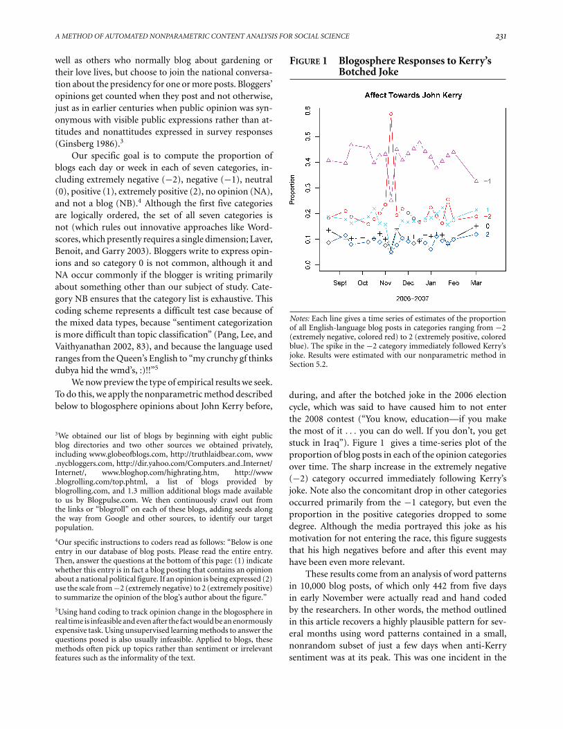
FIGURE 1 Blogosphere Responses to Kerry’sBotched Joke

Notes: Each line gives a time series of estimates of the proportionof all English-language blog posts in categories ranging from −2(extremely negative, colored red) to 2 (extremely positive, coloredblue). The spike in the −2 category immediately followed Kerry’sjoke. Results were estimated with our nonparametric method inSection 5.2.

during, and after the botched joke in the 2006 electioncycle, which was said to have caused him to not enterthe 2008 contest (“You know, education—if you makethe most of it . . . you can do well. If you don’t, you getstuck in Iraq”). Figure 1 gives a time-series plot of theproportion of blog posts in each of the opinion categoriesover time. The sharp increase in the extremely negative(−2) category occurred immediately following Kerry’sjoke. Note also the concomitant drop in other categoriesoccurred primarily from the −1 category, but even theproportion in the positive categories dropped to somedegree. Although the media portrayed this joke as hismotivation for not entering the race, this figure suggeststhat his high negatives before and after this event mayhave been even more relevant.

These results come from an analysis of word patternsin 10,000 blog posts, of which only 442 from five daysin early November were actually read and hand codedby the researchers. In other words, the method outlinedin this article recovers a highly plausible pattern for sev-eral months using word patterns contained in a small,nonrandom subset of just a few days when anti-Kerrysentiment was at its peak. This was one incident in the


run-up to the 2008 campaign, but it gives a sense of thewidespread applicability of the methods. Although we donot offer these in this article, one could easily imaginemany similar analyses of political or social events wherescale or resource constraints make it impossible to con-tinuously read and manually categorize texts. We offermore formal validation of our methods below.

Representing Text Statistically

We now explain how to represent unstructured text asstructured variables amenable to statistical analysis, firstby coding variables and then via statistical notation.

Coding Variables

To analyze text statistically, we represent natural languageas numerical variables following standard procedures(Joachims 1998; Kolari, Finin, and Joshi 2006; Manningand Schutze 1999; Pang, Lee, and Vaithyanathan 2002).For example, for our key variable, we summarize a docu-ment (a blog post) with its category. Other variables arecomputed from the text in three additional steps, each ofwhich works without human input, and all of which aredesigned to reduce the complexity of text.

First, we drop non-English-language blogs (Cavnarand Trenkle 1994), as well as spam blogs (with a tech-nology we do not share publicly; for another, see Ko-lari, Finin, and Joshi 2006). For the purposes of thisarticle, we focus on blog posts about President GeorgeW. Bush (which we define as those that use the terms“Bush,” “George W.,” “Dubya,” or “King George”) andsimilarly for each of the 2008 presidential candidates. Wedevelop specific filters for each person of interest, en-abling us to exclude others with similar names, such as toavoid confusing Bill and Hillary Clinton. For our presentmethodological purposes, we focus on 4,303 blog postsabout President Bush collected February 1–5, 2006, and6,468 posts about Senator Hillary Clinton collected Au-gust 26–30, 2006. Our method works without filtering(and in foreign languages), but filters help focus the lim-ited time of human coders on the categories of interest.

Second, we preprocess the text within each docu-ment by converting to lowercase, removing all punctua-tion, and stemming by, for example, reducing “consist,”“consisted,” “consistency,” “consistent,” “consistently,”“consisting,” and “consists” to their stem, which is “con-sist.” Preprocessing text strips out information, in addi-tion to reducing complexity, but experience in this liter-

ature is that the trade-off is well worth it (Porter 1980;Quinn et al. 2009).

Finally, we summarize the preprocessed text as di-chotomous variables, one type for the presence or absenceof each word stem (or “unigram”), a second type for eachword pair (or “bigram”), a third type for each word triplet(or “trigram”), and so on to all “n-grams.” This defini-tion is not limited to dictionary words. In our application,we measure only the presence or absence of stems ratherthan counts (the second time the word “awful” appearsin a blog post does not provide as much informationas the first). Even so, the number of variables remain-ing is enormous. For example, our sample of 10,771 blogposts about President Bush and Senator Clinton includes201,676 unique unigrams, 2,392,027 unique bigrams, and5,761,979 unique trigrams. The usual choice to simplifyfurther is to consider only dichotomous stemmed uni-gram indicator variables (the presence or absence of eachof a list of word stems), which we have found to work well.We also delete stemmed unigrams appearing in fewer than1% or greater than 99% of all documents, which results in3,672 variables. These procedures effectively group the in-finite range of possible blog posts to “only” 23,672 distincttypes. This makes the problem feasible but still representsa huge number (larger than the number of elementaryparticles in the universe).

Researchers interested in similar problems in com-puter science commonly find that “bag of words” sim-plifications like this are highly effective (e.g., Pang, Lee,and Vaithyanathan 2002; Sebastiani 2002), and our anal-ysis reinforces that finding. This seems counterintuitiveat first, since it is easy to write text whose meaning islost when word order is discarded (e.g., “I hate Clinton.I love Obama”). But empirically, most text sources makethe same point in enough different ways that representingthe needed information abstractly is usually sufficient. Asan analogy, when channel surfing for something to watchon television, pausing for only a few hundred millisecondson a channel is typically sufficient; similarly, the negativecontent of a vitriolic post about President Bush is usu-ally easy to spot after only a sentence or two. When thebag of words approach is not a sufficient representation,many procedures are available: we can code where eachword stem appears in a document, tag each word withits part of speech, or include selective bigrams, such asby replacing “white house” with “white house” (Das andChen 2001). We can also use counts of variables or codevariables to represent meta-data, such as the URL, title,blogroll, or whether the post links to known liberal orconservative sites (Thomas, Pang, and Lee 2006). Manyother similar tricks suggested in the computer science


literature may be useful for some problems (Pang andLee 2008), and all can be included in the methodologydescribed below, but we have not found them necessaryfor the many applications we have tried to date.

Notation and Quantities of Interest

Our procedures require two sets of text documents. Thefirst is a small labeled set , for which each document i(i = 1, . . . , n) is labeled with one of the given categories,usually by reading and hand coding (we discuss how largen needs to be in the sixth section, and what to do if handcoders are not sufficiently reliable in the appendix). Wedenote the Document category variable as Di , which ingeneral takes on the value Di = j , for possible categoriesj = 1, . . . , J .6 (In our running example, Di takes onthe potential values {−2, −1, 1, 0, 1, 2, NA, NB}.) Wedenote the second, larger population set of documentsas the inferential target, and in which each document �

(for � = 1, . . . , L ) has an unobserved classification D�.Sometimes the labeled set is a sample from the populationand so the two overlap; more often it is a nonrandomsample from a different source than the population, suchas from earlier in time.

All other information is computed directly from thedocuments. To define these variables for the labeled setdenote Sik as equal to 1 if word Stem k (k = 1, . . . , K ) isused at least once in document i (for i = 1, . . . , n) and0 otherwise (and similarly for the population set, sub-stituting index i with index �). This makes our abstractsummary of the text of document i the set of these vari-ables, {Si1, . . . , Si K }, which we summarize as the K × 1vector of word stem variables Si . We refer to Si as a wordstem profile since it provides a summary of all the wordstems (or other information) used in a document.

The quantity of interest in most of the supervisedlearning literature is the set of individual classifications forall documents in the population, {D1, . . . , DL }. In con-trast, the quantity of interest for most content analyses insocial science is the aggregate proportion of all (or a subsetof all) of these population documents that fall into eachcategory: P (D) = {P (D = 1), . . . , P (D = J )}′ whereP(D) is a J × 1 vector, each element of which is a pro-portion computed by direct tabulation:

P (D = j ) = 1

L

L∑�=1

1(D� = j ), (1)

6This notation is from King and Lu (2008), who use related methodsapplied to unrelated substantive applications that do not involvecoding text, and different mnemonic associations.

where 1(a) = 1 if a is true and 0 otherwise. Documentcategory Di is one variable with many possible values,whereas word profile Si constitutes a set of dichotomousvariables. This means that P(D) is a multinomial distri-bution with J possible values and P (S) is a multinomialdistribution with 2K possible values, each of which is aword stem profile.

Issues with Existing Approaches

This section discusses problems with two common meth-ods that arise when they are used to estimate social aggre-gates rather than individual classifications.

Existing Approaches

A simple way of estimating P(D) is direct sampling : iden-tify a well-defined population of interest, draw a randomsample from the population, hand code all the documentsin the sample, and count the documents in each category.This method requires basic sampling theory, no abstractnumerical summaries of any text, and no classificationsof individual documents in the unlabeled population.

The second approach to estimating P(D), the aggre-gation of individual document classifications, is standardin the supervised learning literature. The idea is to firstuse the labeled sample to estimate a functional relation-ship between document category D and word featuresS. Typically, D serves as a multicategory dependent vari-able and is predicted with a set of explanatory variables{Si1, . . . , Si K }, using some statistical, machine learning,or rule-based method (such as multinomial logit, regres-sion, discriminant analysis, radial basis functions, CART,random forests, neural networks, support vector ma-chines, maximum entropy, or others). Then the coeffi-cients of the model are estimated, and both the coeffi-cients and the data-generating process are assumed thesame in the labeled sample as in the population. Thecoefficients are then used with the features measured inthe population, S�, to predict the classification for eachpopulation document D�. Social scientists then aggregatethe individual classifications via equation (1) to estimatetheir quantity of interest, P(D).

Problems

Unfortunately, as Hand (2006) points out, the standardsupervised learning approach to individual document


classification will fail in two circumstances, both of whichappear common in practice. (And even if classificationsucceeds with high or optimal accuracy, the next subsec-tion shows that estimating population proportions canstill be biased.)

First, when the labeled set is not a random samplefrom the population, both methods fail. Yet “in many,perhaps most real classification problems the data pointsin the [labeled] design set are not, in fact, randomly drawnfrom the same distribution as the data points to whichthe classifier will be applied. . . . It goes without sayingthat statements about classifier accuracy based on a falseassumption about the identity of the [labeled] design setdistribution and the distribution of future points may wellbe inaccurate” (Hand 2006, 2). Deviations from random-ness may occur due to “population drift,” which occurswhen the labeled set is collected at one point and meant toapply to a population collected over time (as with blogs),or for other reasons. The burdens of hand coding becomeespecially apparent when considering the typical analysiswithin subgroups and the need for a separate randomsample within each.

Second, the data-generation process assumed by thestandard supervised learning approach predicts D with S,modeling P (D | S), but the world works in reverse. Forour running example, bloggers do not start writing andonly afterwards discover their affect toward the president:they start with a view, which we abstract as a documentcategory, and then set it out in words. That is, the rightdata-generation process is the inverse of what is beingmodeled, where we should be predicting S with D, andinferring P (S | D). The consequence of using P (D | S)instead (and without Bayes Theorem, which is not veryhelpful in this case) is the requirement of two assump-tions needed to generalize from the labeled sample tothe population. The first is that S “spans the space of allpredictors” of D (Hand 2006, 9), which means that onceone controls for the measured variables, there exists noother variable that could improve predictive power. Inproblems involving human language, this assumption isnot met, since S is intentionally an abstraction and so bydefinition does not represent all existing information inthe predictors. The other assumption is that the class ofmodels chosen for P (D | S) includes the “true” model.This is a more familiar assumption to social scientists, butit is no easier to meet. In this case, finding even the bestmodel or a good model, much less the “true one,” is a dif-ficult and time-consuming task given the huge numberof potential explanatory variables coded from text andpotential models to run. As Hand writes, “Of course, itwould be a brave person who could confidently assert thatthese two conditions held” (2006, 9).

Optimizing for a Different Goal

Here we show that even optimal individual documentclassification that meets all the assumptions of the last sec-tion can lead to biased estimates of the document categoryproportions. The criterion for success in the classificationliterature, the percent correctly classified in a test set, isobviously appropriate for individual-level classification,but it can be seriously misleading when characterizingdocument populations. For example, of the 23 modelsestimated by Pang, Lee, and Vaithyanathan (2002), thepercent correctly predicted ranges from 77% to 83%. Thisis an excellent classification performance for sentimentanalysis, but suppose that all the misclassifications werein a particular direction for one or more categories. Inthat situation, the statistical bias (the average differencebetween the true and estimated proportion of documentsin a category) in using this method to estimate the ag-gregate quantities of interest could be as high as 17 to23 percentage points. This does not matter for the authors,since their goal was classification, but it could matter forresearchers interested in category proportions.

Unfortunately, except at the extremes, there exists nonecessary connection between low misclassification ratesand low bias: it is easy to construct examples of learningmethods that achieve a high percent of individual docu-ments correctly predicted and large biases for estimatingthe aggregate document proportions, or other methodsthat have a low percent correctly predicted but neverthe-less produce relatively unbiased estimates of the aggregatequantities. For example, flipping a coin is a bad predictorof which party will win a presidential election, but it doeshappen to provide an unbiased estimate of the percentageof Democratic presidential victories since 1912. Since thegoal of this literature is individual classification, it doesnot often report the bias in estimating the aggregates.As such, the bulk of the otherwise impressive supervisedlearning classification literature offers little indication ofwhether the methods proposed would work well for thosewith different goals.

Statistically Consistent Estimatesof Social Aggregates

We now introduce a method optimized for estimatingdocument category proportions. To simplify the exposi-tion, we first show how to correct aggregations of anyexisting classification method and after offer our stand-alone procedure, not requiring (or producing) a methodof individual document classification.


Corrected Aggregations of IndividualClassifications

Intuition. Consider multinomial logit or any othermethod which can generate individual classifications. Fitthis model to the labeled set, use it to classify each ofthe unlabeled documents in the population of interest,and aggregate the classifications to obtain a raw, uncor-rected estimate of the proportion of documents in eachcategory. Next, estimate misclassification probabilities byfirst dividing the labeled set of documents into a train-ing set and a test set (ignoring the unlabeled populationset). Then apply the same classification method to thetraining set alone and make predictions for the test set,Di (ignoring the test set’s labels). Then use the test set’slabels to calculate the specific misclassification probabili-ties between each pair of actual classifications given eachtrue value, P (Di = j | Di = j ′). These misclassificationprobabilities do not tell us which documents are misclas-sified, but they can be used to correct the raw estimate ofthe document category proportions.

For example, suppose we learn, in predicting test setproportions from the training set, that 17% of the docu-ments our method classified as D = 1 really should havebeen classified as D = 3. For any one individual classifi-cation in the population, this fact is of no help. But fordocument category proportions, it is easy to use: subtract17% from the raw estimate of the category 1 proportionin the population, P (D = 1), and add it to category 3,P (D = 3). Even if the raw estimate was badly biased,which can occur despite optimal individual documentclassification, the resulting corrected estimate would beunbiased so long as the population misclassification er-rors were estimated well enough from the labeled set (acondition we discuss below). Even if the percent correctlypredicted is low, this corrected method can give unbiasedestimates of the category frequencies.

Formalization for Two Categories. For the special casewhere D is dichotomous, the misclassification correc-tion above is well known in epidemiology—an area ofscience directly analogous to the social sciences, wheremuch data are at the individual level, but the quantitiesof interest are often at the population level. To see this,consider a dichotomous D, with values 1 or 2, a raw esti-mate of the proportion of documents in category 1 fromsome method of classification, P (D = 1), and the trueproportion (corrected for misclassification), P (D = 1).7

7The raw estimate P (D = 1) can be based on the proportion ofindividual documents classified into category 1. However, a betterestimate for classifiers that give probabilistic classifications is to sum

Then define two forms of correct classification as “sensi-tivity,” sens ≡ P (D = 1 | D = 1) (sometimes known as“recall”), and “specificity,” or spec ≡ P (D = 2 | D = 2).For example, sensitivity is the proportion of documentspredicted to be in category 1 among those actually incategory 1.

Then we note that the proportion of documents es-timated to be in category 1 must come from only one oftwo sources: documents actually in category 1 that werecorrectly classified and documents actually in category 2but misclassified into category 1. We represent this ac-counting identity, known as the Law of Total Probability,as

P (D = 1) = (sens)P (D = 1) + (1 − spec)P (D = 2).

(2)

Since equation (2) is one equation with only oneunknown [since P (D = 1) = 1 − P (D = 2)], it is easyto solve. As Levy and Kass (1970) first showed, the solutionis

P (D = 1) = P (D = 1) − (1 − spec)

sens − (1 − spec). (3)

This expression can be used in practice by estimating sen-sitivity and specificity in the first-stage analysis (separat-ing the labeled set into training and test sets as discussedabove or more formally by cross-validation) and usingthe entire labeled set to predict the (unlabeled) popula-tion set to give P (D = 1). Plugging these values in theright side of (3) gives a corrected, and statistically con-sistent, estimate of the true proportion of documents incategory 1.

Generalization to Any Number of Categories. The ap-plications in epidemiology for which these expressionswere developed are completely different than our prob-lems, but the methods developed there are directly rele-vant. This connection enables us to use for our applicationthe generalizations developed by King and Lu (2008).8

the estimated probability that each document is in the category forall documents. For example, if 100 documents each have a 0.52probability of being in category 1, then all individual classificationsare in this category. However, since we would only expect 52%of documents to actually be in category 1, a better estimate isP (D = 1) = 0.52.

8King and Lu’s (2008) article contributed to the field in epidemiol-ogy called “verbal autopsies.” The goal of this field is to estimate thedistribution of the causes of death in populations without medicaldeath certification. This information is crucial for directing inter-national health policy and research efforts. Data come from twosources. One is a sample of deaths from the population, wherea relative of each deceased is asked a long (50–100 item) list ofusually dichotomous questions about symptoms the deceased may


Thus, we first generalize equation (2) to include any num-ber of categories by substituting j for 1, and summing overall categories instead of just 2:

P (D = j ) =J∑

j ′=1

P (D = j | D = j ′)P (D = j ′). (4)

Given P (D) and the misclassification probabilitiesP (D = j | D = j ′), which generalize sensitivity andspecificity to multiple categories, this expression repre-sents a set of J equations (i.e., defined for j = 1, . . . , J )that can be solved for the J elements in P(D). This isaided by the fact that the equations include only J − 1unknowns since elements of P(D) must sum to 1.

Interpretation. The section entitled “Optimizing fora Different Goal” shows that a method meeting all theassumptions required for optimal classification perfor-mance can still give biased estimates of the documentcategory proportions. We therefore offer here statisticallyconsistent estimates of document category proportions,without having to improve individual classification ac-curacy and with no assumptions beyond those alreadymade by the individual document classifier. In particu-lar, classifiers require that the labeled set be a randomsample from the population. Our method only requiresa special case of the random selection assumption: thatthe misclassification probabilities (sensitivity and speci-ficity with 2 categories or P (D = j | D = j ′) for all jand j

′in equation (4)) estimated with data from the la-

beled set also hold in the unlabeled population set. Thisassumption may be wrong, but if it is, then the assump-tions necessary for the original classifier to work are alsowrong and will not necessarily even give accurate individ-ual classifications. More importantly, our approach willalso work with a biased classifier.

Document Category Proportions WithoutIndividual Classifications

We now offer an approach that requires no parametricstatistical modeling, individual document classification,or random sampling from the target population. It also

have suffered prior to death (S�). The other source of data is deathsin a nearby hospital, where the same data collection of symptomsfrom relatives is collected (Si ) and also where medical death cer-tification is available (Di ). Their method produces approximatelyunbiased and consistent estimates, considerably better than the ex-isting approaches, which included expensive and unreliable physi-cian reviews (where three physicians spend 20 minutes with theanswers to the symptom questions from each deceased to decideon the cause of death), reliable but inaccurate expert rule-basedalgorithms, or model-dependent parametric statistical models.

correctly treats S as a consequence rather than cause ofD.

The Approach. This method requires only one addi-tional step beyond that in the previous section: instead ofusing S and D to estimate P (D = j ), and then separatelycorrecting via equation (4), we avoid having to computeD by using S in place of D in that same equation. Thatis, any observable implication of D can be used in placeof D in equation (4); because D is a function of S—sincethe words chosen are by definition a function of the doc-ument category—it is simplest to use it directly. Thus, wehave

P (S = s ) =J∑

j=1

P (S = s | D = j )P (D = j ). (5)

To simplify this expression, we rewrite equation (5) as anequivalent matrix expression:

P (S)2K ×1

= P (S | D)2K ×J

P (D)J ×1

(6)

where, as indicated, P (S) is the probability of each of the2K possible word stem profiles occurring,9 P (S | D) is theprobability of each of the 2K possible word stem profilesoccurring within the documents in category D (columnsof P (S | D) corresponding to values of D), and P(D) isour J-vector quantity of interest.

Estimation. Elements of P (S) can be estimated by di-rect tabulation from the target population, without para-metric assumptions: we merely compute the proportionof documents observed with each pattern of word pro-files. Since D is not observed in the population, we cannotestimate P (S | D) directly. Instead, we make the crucialassumption that its value in the labeled, hand-coded sam-ple, P h(S | D), is the same as that in the population,

P h(S | D) = P (S | D), (7)

and use the labeled sample to estimate this matrix (wediscuss this assumption below). We avoid parametric as-sumptions here too, by using direct tabulation to com-pute the proportion of documents observed to have eachspecific word profile among those in each documentcategory.

In principle, we could estimate P(D) in equation (6)assuming only the veracity of equation (7) and the accu-racy of our estimates of P (S) and P (S | D), by solvingequation (6) via standard regression algebra. That is, if we

9For example, if we ran the method with only K = 3 word stems,P (S) would contain the probabilities of each of these (23 = 8)patterns occurring in the set of documents: 000 (i.e., none of thethree words were used), 001, 010, 011, 100, 101, 110, and 111.


think of P(D) as the unknown “regression coefficients”�, P (S | D) as the “explanatory variables” matrix X , andP (S) as the “dependent variable” Y , then equation (6) be-comes Y = X� (with no error term). This happens to bea linear expression but not because of any assumptionimposed on the problem that could be wrong. The resultis that we can solve for P(D) via the usual regression cal-culation: � = (X ′ X)−1 X ′y (or via standard constrainedleast squares to ensure that elements of P(D) are each in[0,1] and collectively sum to 1). A key point is that thiscalculation does not require classifying individual docu-ments into categories and then aggregating; it estimatesthe aggregate proportions directly.

This simple approach poses two difficulties in ourapplication. First, K is typically very large and so 2K

is far larger than any standard computer could handle.Second is a sparseness problem since the number of ob-servations available for estimating P (S) and P (S | D) ismuch smaller than the number of potential word pro-files (n << 2K ). To avoid both of these issues, we adaptresults from King and Lu (2008) and randomly choosesubsets of between approximately 5 and 25 words. Theoptimal number of words to use per subset is application-specific, but can be determined empirically through cross-validation within the labeled set. Although the estimatorremains approximately unbiased regardless of subset size,in practice we find that setting the number of words persubset too high can lead to inefficiency. The reason is thatas the number of words per subset increases, the num-ber of unique subsets increases, reducing the number ofcommon subsets that appear in both the labeled and un-labeled data sets. In addition, in the applications below,the words included in each subset are chosen randomlywith equal probabilities, although in some applications,performance may improve by weighting words unequally.

Once we determine the optimal number of subsetsthrough cross-validation, we solve for P(D) in each, andaverage the results across the subsets. Because S is treatedas a consequence of D, using subsets of S introducesno new assumptions. This simple subsetting procedureturns out to be equivalent to a version of the standardapproach of smoothing sparse matrices via kernel densi-ties, although, unlike the typical use of this procedure, itsapplication here reduces bias. (Standard errors and confi-dence intervals are computed via standard bootstrappingprocedures.)

Interpretation. A key advantage of estimating P(D)without the intermediate step of computing the individ-ual classifications is that the required assumptions aremuch less restrictive. They can still be wrong, and as aresult our estimates can be biased, but the dramatic re-

duction in their restrictiveness means that under the newapproach we have a fighting chance to get something closeto the right answer in many applications where valid in-ferences were not previously likely.

Unlike direct sampling or standard supervised learn-ing approaches, our strategy allows the distribution ofdocuments across word-stem profiles, P (S), and the dis-tribution of documents across the categories, P(D), toeach be completely different in the labeled set and pop-ulation set of documents. So for example, if a word orpattern of words becomes more popular between the timethe labeled set was hand coded and the population docu-ments were collected, no biases would emerge. Similarly,if documents in certain categories are more prevalent inthe population than labeled set, no biases would result. Inour running example, no bias would be induced if the la-beled set includes a majority of conservative Republicanswho defend everything President Bush does and the tar-get population has a supermajority of liberal Democratswho want nothing more than to end the Bush presidency.In contrast, changes in either P(D) or P (S) between thelabeled and population sets would be sufficient to doomexisting classification-based approaches. For example, solong as “idiot” remains an insult, our method can makeappropriate use of that information, even if the word be-comes less common (a change in P(S)) or if there arefewer people who think politicians deserve it (a change inP(D)).

The key theoretical assumption is equation (7)—that the documents in the hand-coded set contain suf-ficient good examples of the language used for each doc-ument category in the population. To be more specific,among all documents in a given category, the prevalenceof particular word profiles in the labeled set should bethe same in expectation as in the population set. Forexample, the language bloggers use to describe an “ex-tremely negative” view of Hillary Clinton in the labeledset must be at least a subset of the way she is describedin the target population. They do not need to writeliterally the same blog posts, but rather need to havethe same probabilities of using similar word profiles sothat P h(S | D = −2) = P (S | D = −2). This assump-tion can be violated due to population drift or for otherreasons, but we can always hand code some additionalcases in the population set to verify that it holds suffi-ciently well. And as discussed above, the proportion ofexamples of each document category and of each wordprofile can differ between the two document sets.

The methodology is also considerably easier to usein practice. Applying the standard supervised learningapproach is difficult, even if we meet its assumptions.Even if we forget about choosing the “true” model, merely


finding a “good” specification with thousands of explana-tory variables to choose from can be extraordinarily timeconsuming. One needs to fit numerous statistical mod-els, consider many specifications within each model type,run cross-validation tests, and check various fit statistics.Social scientists have a lot of experience with specificationsearches, but all the explanatory variables mean that evenone run would take considerable tuning and many runswould need to be conducted.

The problem is further complicated by the fact thatsocial scientists are accustomed to choosing their statis-tical specifications on the basis of prior theoretical ex-pectations and results from past research, whereas theoverwhelming experience in the information extractionliterature is that radically empirical approaches work bestfor a given amount of effort. For example, we might thinkwe could carefully choose words or phrases to characterizeparticular document categories (e.g., “awful,” “irrespon-sible,” “impeach,” etc., to describe negative views aboutPresident Bush), and indeed this approach will often workto some degree. Yet, a raw empirical search for the bestspecification, ignoring these theoretically chosen words,will typically turn up predictive patterns we would nothave thought of ex ante. Indeed, methods based on highlydetailed parsing of the grammar and sentence structurein each document can also work exceptionally well (e.g.,King and Lowe 2003), but the strong impression from theliterature is that the extensive, tedious work that goes intoadapting these approaches for each application is moreproductively put into collecting more hand-coded ex-

amples and then using an automatic specification searchroutine.

The Method in Practice

We begin here with a simple simulated example, proceedto real examples of different types of documents, andstudy how many documents one needs to hand code.We also compare our approach to existing methods anddiscuss what can go wrong. Readers can replicate andmodify any of these analyses using the replication filesmade available with this article.

Monte Carlo Simulations

We begin with a simulated data set of 10 words and thus210 = 1,024 possible word-stem profiles. We set the ele-ments of P h(D) to be the same across the seven categories,and then set the population document category frequen-cies, P(D), to very different values. We then draw a valueD from P h(D), insert the simulation into P h(S | D),which we set to that from the population, and then drawthe simulated matrix S from this density. We repeat theprocedure 1,000 times to produce the labeled data set,and analogously for the population.

The left two panels of Figure 2 summarize the sharpdifferences between the hand-coded and population

FIGURE 2 Accurate Estimates Despite Differences Between Labeled and Population Sets

Notes: For both P (D) on the left and P (S) in the center, the distributions differ considerably. The direct sampling estimator, P h(D), istherefore highly biased. Yet, the right panel shows that our nonparametric estimator remains unbiased.


distributions in these data. The left graph plots P h(D)horizontally by P(D) vertically, where the seven circlesrepresent the category proportions. If the proportionswere equal, they would all fall on the 45◦ line. If one usedthe labeled, hand-coded sample in this case via directsampling to estimate the document category frequenciesin the population, the result would not even be positivelycorrelated with the truth.

The differences between the two distributions of wordfrequency profiles appear in the middle graph (wherefor clarity the axes, but not labels, are on the log scale).Each circle in this graph represents the proportion ofdocuments with a specific word profile. Again, if the twodistributions were the same, all the circles would appearon the diagonal line, but again many of the circles fall offthe line, indicating differences between the two samples.

Despite the considerable differences between the la-beled data set and the population, and the bias in thedirect sampling estimator, our approach still producesaccurate estimates. The right panel of the figure presentsthese results. The actual P(D) is on the horizontal axis andthe estimated version is on the vertical axis, with each ofthe seven circles representing one of the document fre-quency categories. Estimates that are accurate fall on the45◦ line. In fact, the points are all huddled close to thisequality line, with even the maximum distance from theline for any point being quite small.

Empirical Evidence

We now offer several out-of-sample tests of our nonpara-metric approach in different types of real data. Our firsttest includes the 4,303 blog posts that mention GeorgeW. Bush. (For levels of intercoder reliability for this task,see the appendix.) These posts include 47,726 uniquewords and 3,165 unique word stems. We randomly di-vide the data set in half between the training set and testset and, to make the task more difficult, then randomlydelete half (422) of the posts coded −2 in the test set. Ourtest set therefore intentionally selects on (what would beconsidered, in standard supervised learning approaches)the dependent variable. The results from our nonpara-metric estimator appear in Figure 3 as one open circlefor each of the seven categories, with 95% confidenceintervals appearing as a vertical line. Clearly the pointsare close to the 45◦ line, indicating approximately un-biased estimates, and all are within the 95% confidenceintervals.

Also plotted on the same graph are the documentcategory proportions aggregated up from individual clas-

FIGURE 3 Out-of-Sample Validation

●●

●● ●●

●

●

0.0 0.2 0.4 0.6 0.8 1.00.

00.

20.

40.

60.

81.

0

Affect in Blogs

Actual P(D)

Est

imat

ed P

(D)

●

●

●●●

●

●

0.0 0.2 0.4 0.6 0.8 1.00.

00.

20.

40.

60.

81.

0

Affect in Blogs

Actual P(D)

Est

imat

ed P

(D)

0.0 0.2 0.4 0.6 0.8 1.00.

00.

20.

40.

60.

81.

0

Affect in Blogs

Actual P(D)

Est

imat

ed P

(D)

0.0 0.2 0.4 0.6 0.8 1.00.

00.

20.

40.

60.

81.

0

Affect in Blogs

Actual P(D)

Est

imat

ed P

(D)

0.0 0.2 0.4 0.6 0.8 1.00.

00.

20.

40.

60.

81.

0

Affect in Blogs

Actual P(D)

Est

imat

ed P

(D)

Notes: The plot gives the estimated document category frequencies(vertically) by the actual frequencies (horizontally). Our nonpara-metric approach is represented with black open circles, with 95%confidence intervals as vertical lines. Aggregated optimized SVManalyses also appear for radial basis (black dots), linear (green tri-angles), polynomial (blue diamonds), and sigmoid kernels (redsquares). Estimates closer to the 45◦ line are more accurate.

sifications given by four separately optimized supportvector machine (SVM) classifiers, the most widely used(and arguably the best) of the existing methods. Theseinclude SVMs using a radial basis function (black dots),linear kernel (green triangles), polynomial kernel (bluediamonds), and sigmoid kernel (red squares) (Branket al. 2002; Hastie, Tibshirani, and Friedman 2001; Hsu,Chang, and Lin 2003; Joachims 1998). As can be seenin the graph, these results vary wildly and none do aswell as our approach. They are plotted without confi-dence intervals since SVM is not a statistical method andhas no probabilistic foundation. An additional difficultyof using individual classifiers is the highly time-intensivetuning required. Whereas the results from our approachrepresent only a single run, we followed the advice of theSVM literature and chose the final four SVMs to presentin Figure 3 by optimizing over a total of 19,090 separateSVM runs, including cross-validation tests on 10 separatesubsets of the labeled set. One run of our nonparametricestimator took 60 seconds of computer time, or a totalof five hours for 300 bootstrapped runs. The SVM runs


TABLE 1 Performance of Our Nonparametric Approach and Four Support Vector MachineAnalyses

Percent of Blog Posts Correctly Classified

In-Sample In-Sample Out-of-Sample Mean AbsoluteFit Cross-Validation Prediction Proportion Error

Nonparametric — — — 1.2Linear 67.6 55.2 49.3 7.7Radial 67.6 54.2 49.1 7.7Polynomial 99.7 48.9 47.8 5.3Sigmoid 15.6 15.6 18.2 23.2

Notes: Each row is the optimal choice over numerous individual runs given a specific kernel. Leaving aside the sigmoid kernel, individualclassification performance in the first three columns does not correlate with mean absolute error in the document category proportions inthe last column.

took approximately 8.7 days (running 24 hours/day) ona powerful server and much more in human time.

We give an alternative view of these results in Table 1.The first three numerical columns report individual clas-sification performance whereas the last gives the meanabsolute error in the document category proportions. Thelast column confirms the overall impression from Figure3 that the nonparametric method has much lower error inestimating the document category proportions. Leavingaside the sigmoid kernel, which did not work well in thesedata, the SVM results have the familiar patterns for indi-vidual classifiers: the models fit best to the in-sample data,followed next by in-sample cross-validation, and lastly bythe true out-of-sample predictions. The key result in thisanalysis is that, even among the SVM analyses, the bestindividual classifier (the linear kernel) is different fromthe best choice for minimizing the mean absolute errorin the document category proportions (the polynomialkernel). Of course, nothing is wrong with SVM when ap-plied to the individual classification goal for which it wasdesigned.

Examples from Other Textual Data Sources

We now give three brief examples applying our methodto different sources of unstructured text. The first is froma corpus of congressional speeches used in the computerscience literature to evaluate supervised learning methods(Thomas, Pang, and Lee 2006). Researchers selected 3,838speeches given in the House of Representatives betweenJanuary 4th and May 12th, 2005, during “contentious”debates, defined as those where more than 20% of thespeeches were in opposition. To simulate how a resource-conscious researcher might proceed, we used the 1,887

speeches appearing on even-numbered pages of the con-gressional record as a training set, and then estimated thedistribution of supportive speeches in the test set of 1,951speeches on odd-numbered pages. The results using thenonparametric estimator appear in the top-left graph inFigure 4 and are again highly accurate.

Another example comes from a data set of 462 immi-gration editorials that we compiled using Factiva. The ed-itorials appeared in major newspapers between April 1stand July 15th, 2007, and were coded into four nonorderedcategories indicating editorials supporting the Senate’simmigration bill, those opposing it, and two categoriesthat capture letters to the editor and other miscellaneousarticles. Here, the training set includes the 283 editorialsprior to June 12th, while the test set includes the 179 edi-torials on or after that date. Deviations from the 45◦ lineare due to slight violations of the assumption in equation(7). This is quite a hard test, since some categories haveas few as 40 examples. The small discrepancy can also befixed easily if this were a real application by adding to thehand-coded set a small number of documents collectedover time.

Our final example comes from 1,726 emails sent byEnron employees and classified into five nonordered cat-egories: company business, personal communications,logistic arrangements, employment arrangements, anddocument editing.10 To make the task more difficult,we first created a skewed test set of 600 emails that wasmore uniformly distributed than the training set, with nocategory accounting for less than 12% or more than 39%of the observations. We then used the remaining 1,126emails as a mutually exclusive training set where the com-parable bounds were 4% and 50%. The results are quite

10See http://www.cs.cmu.edu/∼enron/.


FIGURE 4 Additional Out-of-Sample Validation

●

●

0.0 0.2 0.4 0.6 0.8

0.0

0.2

0.4

0.6

0.8

Actual P(D)

Est

imat

ed P

(D)

●

●

●

●

0.0 0.1 0.2 0.3 0.4 0.5 0.6

0.0

0.1

0.2

0.3

0.4

0.5

0.6

Actual P(D)E

stim

ated

P(D

)

●

●

●

●●

0.0 0.2 0.4 0.6 0.8

0.0

0.2

0.4

0.6

0.8

Actual P(D)

Est

imat

ed P

(D)

Notes: The left graph displays the accuracy of the nonparametric method in recovering the distribution of supporting versus opposingspeeches in Congress. The center graph shows the same for a categorization of newspaper editorials on immigration, and the rightgraph shows the distribution across categories of emails sent by enron employees. As before, 95% confidence intervals are representedby vertical lines, and estimates closer to the 45◦ line are more accurate.

accurate, especially given the paucity of information inmany (short) emails, and are displayed in the right panelof Figure 4.

How Many Documents Needto Be Hand Coded?

Any remaining bias in our estimator is primarily a func-tion of the assumption in equation (7). In contrast, effi-ciency, as well as confidence intervals and standard errors,are primarily a function of how many documents are handcoded and so are entirely under the control of the investi-gator. But how many is enough? Hand coding is expensiveand time consuming and so we would want to limit itsuse as much as possible, subject to acceptable uncertaintyintervals.

To study this question, we set aside bias by randomlysampling the labeled set directly from the population andplotting in Figure 5 the root mean square error (RMSE)averaged across the categories vertically by the numberof hand-coded documents horizontally for our estimator(solid line) and the direct sampling estimator (dashedline). RMSE is lower for the direct estimator, of course,since this sample was drawn directly from the populationand little computation is required, although the differencebetween the two is only about two-tenths of a percentagepoint.

For our estimator, the RMSE drops quickly as thenumber of hand-coded documents increases. Even thehighest RMSE, with only 100 documents in the labeled

FIGURE 5 Average Root Mean Square Errorby Number of Hand-CodedDocuments

200 400 600 800 1000

0.00

0.01

0.02

0.03

0.04

200 400 600 800 1000

0.00

0.01

0.02

0.03

0.04

Number of Hand-Coded Documents

Avg

. Roo

t Mea

n S

quar

ed E

rror

set, is only slightly higher than 3 percentage points, whichwould be acceptable for some applications. (For example,most national surveys have a margin of error of at least 4percentage points, even when assuming random samplingand excluding all other sources of error.) At about 500documents, the advantage of more hand coding begins to


suffer diminishing returns. In part this is because there islittle more error to eliminate as our estimator then has anaverage RMSE of only about 1.5 percentage points.

The conclusion here is clear: coding more than about500 documents to estimate a specific quantity of interestis probably not necessary, unless one is interested in muchmore narrow confidence intervals than is common or inspecific categories that happen to be rare. For some appli-cations, as few as 100 documents may even be sufficient.

What Can Go Wrong?

We now discuss five problems that can arise with ourmethods. If they do arise, and steps are not taken to avoidor ameliorate them, they can cause our estimator to bebiased or inefficient. We also discuss what to do to ame-liorate these problems.

First, and most importantly, our procedure cannotwork without reliable information. This requires that theoriginal documents contain the information needed, thehand codings are reliable enough to extract the informa-tion from the documents, and the quantitative summaryof the document (in S) is a sufficiently accurate represen-tation and sufficient to estimate the quantities of interest.Each of these steps requires careful study. Documentsthat do not contain the information needed cannot beused to estimate quantities of interest. If humans can-not code these documents into well-defined categorieswith some reasonable level of reliability, then automatedprocedures are unlikely to succeed at the same task. Andmany choices are available in producing abstract numer-ical summaries of written text documents. Although wehave found that stemmed unigrams are a sufficient rep-resentation to achieve approximately unbiased inferencesin our examples, researchers may have to use some ofthe other tricks discussed in the section entitled “codingvariables” for different applications.

Second, a key issue is the assumption in equation(7) that P (S | D) is the same in the labeled and popu-lation document sets. We thus have much less restrictiveassumptions than prior methods, but we still assume aparticular type of connection between the two documentsets. If we are studying documents over a long time period,where the language used to characterize certain categoriesis likely to change, it would not be advisable to select thelabeled test set only from the start of the period. Check-ing whether this assumption holds is not difficult andmerely requires hand coding some additional documentscloser to the quantity presently being estimated and us-ing them as a validation test set. If the data are collected

over time, one can either hand code several data sets fromdifferent time periods or gradually add hand-coded doc-uments collected over time. In our running example, weare attempting to track opinions over a single presidentialcampaign. As such, only one hand-coded data set at thestart may be sufficient, but we have tested this assumption,and will continue to do so by periodically hand codingsmall numbers of blogs.11

Third, each category of D should be defined so as tobe mutually exclusive, exhaustive, and relatively homo-geneous. To confront cases where the categories are notmutually exclusive, one can define an additional “both”category. Categories that require many examples to definemay be too broad for effective estimation as may occurfor residual or catch-all categories. Consider the “NB”category in our data as one example. There are innumer-able types of web sites that are not blogs, each with verydifferent language; yet this category was essential sinceour blog search algorithm was not perfect. In fact, we dofind slightly more bias in estimating category NB than theothers in our categorization, but not so much as to causea problem for our applications. Given our experiences,the identification of an effective set of categories in D isan important issue and should involve careful iterationbetween improving concepts, validation in hand codingtests, and searching for new possibilities in example doc-uments. Intercoder reliability is a crucial metric as well. Ifhuman coders cannot agree on a classification, automatedapproaches are not likely to return sensible results either.

Fourth, our approach requires the choice of the num-ber of word stems to use in each randomly chosen subset.While choosing the number of random subsets is easy(the more the better, and so like any simulation methodthe number should be chosen based on available com-puter time and the precision needed), the number ofword stems to use in each random subset must be cho-sen more carefully. Choosing too few or too many willleave P (S) and P (S | D) too sparse or too short and mayresult in attenuation bias due to measurement error inP (S | D), which serve as the “explanatory variables” inthe estimation equation. To make this choice in practice,we use standard automated cross-validation techniques,such as by randomly dividing the labeled set into trainingand test sets and then checking what works in those data.

11To generate a clear example of where this assumption is violated,we divided a test set into subsets based on the sophistication of thelanguage using Flesch-Kincaid scores, which attempt to measurethe grade level needed to read a text. We then tried to estimate thedocument category frequencies from a labeled set that made nosuch distinctions. Since the language sophistication is computeddirectly from the document text, equation (7) was violated and ourestimates were biased as a result.


In practice, the number of word stems to choose to avoidsparseness bias mainly seems to be a function of the num-ber of unique word stems in the documents. Fixing anyproblem that may arise via these types of cross-validationtests is not difficult. Given the other recommendationsdiscussed above—stability in P (S | D), coding categoriesthat are homogeneous and clearly defined—the choice ofthe optimal number of subsets can account for many ofthe performance problems we observe in practice. In someapplications, researchers may find it helpful to weight theword stems unevenly, so that words likely to have more in-formation (such as based on their “mutual information”)appear more frequently in the subsets, although we havenot found this necessary.

Finally, we require a reasonable number of docu-ments in each category of D to be hand coded. Althoughwe studied the efficiency of our procedure as a functionof the number of hand-coded documents above, these re-sults would change if by chance some categories had veryfew hand-coded documents and we cared about smalldifferences in the proportions in these population cat-egories. This makes sense, of course, since the methodrequires examples from which to generalize. Discoveringtoo few examples for one or more categories can be dealtwith in several ways. Most commonly, one can alter thedefinition of the categories or can change the coding rules.

However, even if examples of some categories arerare, they may be sufficiently well represented in the muchlarger population set to be of interest to social scientists.To deal with situations like this, we would need to findmore examples from these relatively rare categories. Do-ing so by merely increasing the size of the hand-coded dataset would be wasteful given that we would wind up withmany more coded documents in the more prevalent cate-gories. Still, it may be possible to use available meta-datato find the needed documents with higher probability. Inour blogs data, we could find blog posts of certain typesvia links from other already hand-coded posts or frompopular directories of certain types of blogs. Fortunately,the labeled set is assumed to be generated conditional onthe categories, and so no bias is induced if we add extraexamples via this “case-control” approach (cf. King andZeng 2002).

Throughout all these potential problems, the bestapproach seems to be the radically empirical proceduresuggested in the supervised learning literature. If the pro-cedure you choose works, it works; if it doesn’t, it doesn’t.And so one should verify that the procedures work bysubdividing the labeled set into training and (truly outof sample) test sets and then directly testing hypothesesabout the success of the procedure. Ideally, this should

then be repeated with different types of labeled test sets.The more we make ourselves vulnerable to being wrong,using rigorous scientific procedures, the more we learn.Fortunately, the tools we make available here would seemto make it possible to learn enough to produce a reliableprocedure in many applications.

Relatedly, standard errors and confidence intervalstake a very different role in this type of research thanthe typical observational social science work. For mostmethods, the only way to shrink confidence intervals isto collect more data. For the method introduced here, alla researcher needs to do is to hand code additional doc-uments (selected randomly or randomly conditional onD) and rerun the algorithm. As long as no data are dis-carded along the way, continuing to hand code until one’sconfidence intervals are small enough induces no bias,since our methodology (like direct sampling) is invariantto sampling plans (Thompson 2002, 286ff). A reasonablygeneral approach is to hand code roughly 200 documentsand run the algorithm. If uncertainty is more than desired,then hand code 100 more randomly selected documents,add them to the first set, reestimate, and continue untilthe uncertainty is small enough.

Given the many possible applications of this method,it is difficult to provide general guidelines about howtime-intensive the entire process is likely to be. However,our experience is that identifying clear categories that hu-mans are consistently able to differentiate takes far longerthan the automated analyses we propose. Once users haveclearly defined categories hand coded for a few hundreddocuments, they can often estimate the document cate-gory proportions for far larger corpora a few hours later.

Concluding Remarks

Existing supervised methods of analyzing textual datacome primarily from the tremendously productive com-puter science literature. This literature has been focusedon optimizing the goals of computer science, which forthe most part involve maximizing the percent of docu-ments correctly classified into a given set of categories.We do not offer a way to improve on the computer sci-entists’ goals. Instead of seeking to classify any individualdocument, most social science literature that has hand-(or computer-) coded text is primarily interested in broadcharacterizations about the whole set of documents, suchas unbiased estimates of the proportion of documents ingiven categories. Unfortunately, since they are optimizedfor a different purpose, computer science methods oftenproduce biased estimates of these category proportions.


By developing methods for analyzing textual data thatoptimize social science goals directly, we are able to con-siderably outperform standard computer science meth-ods developed for a different purpose. In addition, ourapproach requires no modeling assumptions, no model-ing choices, and no complicated statistical approaches,and lets the social scientist pose the theoretical ques-tion to be answered. It also requires far less work thanprojects based entirely on hand coding, and much lesswork than most computer science methods of individ-ual classification; it is both fast and can be used in realtime. Individual-level classification is not a result of thismethod, and so it is not useful for all tasks, but numerousquantities of interest, from separate subdivisions of thepopulation or different populations, can be estimated. Aswith all supervised learning methods, our approach doesrequire careful efforts to properly define categories andto hand code a small sample of texts.

Although we have included only a few applications inthis article, the methods offered here would seem appli-cable to many possible analyses that may not have beenfeasible previously. With the explosion of numerous typesand huge quantities of text available to researchers on theweb and elsewhere, we hope social scientists will beginto use these methods, and develop others, to harvest thisnew information and to improve our knowledge of thepolitical, social, cultural, and economic worlds.

Appendix Correcting for Lackof Intercoder Reliability

Hand coding is often an error-prone task. Intercoder re-liability is measured in many different ways in the litera-ture, but the rates tend to be lower with more categoriesand more theoretically interesting coding schemes andare almost never perfectly reliable. Unfortunately, “theclassical supervised classification paradigm is based onthe assumption that there are no errors in the true classlabels” (Hand 2006, 9). The problem may be due to “con-ceptual stretching” (Collier and Mahon 1993) or “conceptdrift” (Widmer and Kubat 1996) that could in principlebe fixed with a more disciplined study of the categories orcoder training, but in practice some error is always left. Incurrent practice, scholars typically report some reliabilitystatistics and then use methods that assume no misclas-sification. Here, we propose to address misclassificationvia simulation-extrapolation (SIMEX; Cook and Stefan-ski 1994; Kuchenohoff, Mwalili, and Lassaffre 2006).

As an example, before we developed our methods,we had at least two coders categorize each of 4,169 blog

TABLE 2 Intercoder Reliability

−2 −1 0 1 2 NA NB P(D1)

−2 .70 .10 .01 .01 .00 .02 .16 .28−1 .33 .25 .04 .02 .01 .01 .35 .080 .13 .17 .13 .11 .05 .02 .40 .021 .07 .06 .08 .20 .25 .01 .34 .032 .03 .03 .03 .22 .43 .01 .25 .03NA .04 .01 .00 .00 .00 .81 .14 .12NB .10 .07 .02 .02 .02 .04 .75 .45

Notes: This table presents conditional probabilities for coder 2’sclassification (in a set of column entries) given a code assigned bycoder 1 (corresponding to a particular row), or P(D2 | D1). Forinstance, when coder 1 chooses category −2, coder 2 will choosethe same category 70% of the time, category −1 10% of the time,and so on across the first row. This matrix is estimated from all4,169 coding pairs from five coders. The final column denotes themarginal probability that coder 1 placed the blog in each category.

posts. In these data, our coders agreed on the classificationof 66.5% of the blog posts; they agreed on 71.3% of blogposts among those when both coders agreed the post con-tained an opinion; and they agreed on 92% of the posts foran aggregated classification of negative, neutral, or pos-itive opinions among posts with opinions. Table 2 givesmore detailed information. For any two coders, arbitrar-ily named 1 and 2, each row gives the probability of coder2’s classification given a particular classification d chosenby coder 1, P (D2 | D1 = d), with the marginal probabil-ity for coder 1 appearing in the last column, P (D1). The“misclassification” (or “confusion”) matrix in this tableincludes information from all combinations of observedordered coder pairs.

Intuition. For intuition, we illustrate our approachby an analogy to what might occur during a highly fundedresearch project as a coding scheme becomes clearer, thecoding rules improve, and coder training gets better. Forclarity, imagine that through five successive rounds, wehave different, more highly trained coders classifying thesame set of documents with improved coding rules. If wedo well, the results of each round will have higher rates ofintercoder reliability than the last. The final round will bebest, but still not perfect. If we could continue this processindefinitely, we might imagine that we would remove allmisclassification.

Now suppose our estimate of the percent of docu-ments in category 2 is 5% in the first round, 11% in thesecond, 14% in the third, 19% in the fourth, and 23% inthe last round. Following all previously published con-tent analyses, our estimate of the proportion in category2 would be 23%. This is not unreasonable, but it appears


to leave some information on the table. In particular, ifthe proportion of documents in category 2 is increas-ing steadily as the level of intercoder reliability at eachround improves, then we might reasonably extrapolatethis proportion to the point where intercoder agreementis perfect. We might thus conclude that the true propor-tion in category 2 is actually somewhat larger than 23%.We might even formalize this idea by building some typeof regression model to predict the category 2 proportionwith the level of intercoder reliability and extrapolate tothe unobserved point where reliability is perfect. Since thisprocedure involves extrapolation, it is inherently modeldependent and so uncertainty from its inferences will ex-ceed the nominal levels (King and Zeng 2006). However,a crucial point is that even using the figure from the finalround and doing no subsequent processing still involvesan extrapolation; it is just that the extrapolation ignoresthe information from previous rounds of coding. So using23% as our estimate and ignoring this problem is no safer.

Formalization. Following the intuition outlinedabove, we make use of the misclassifications estimatedfrom a single round of coding with more than one coder,simulate what would have happened to the documentcategory proportions if there were even lower levels ofintercoder reliability, and extrapolate back to the point ofno misclassification.

To formalize this SIMEX procedure, begin with ourestimation method, which would give statistically con-sistent answers if it were applied to data with no mis-classification. The same method applied to error-pronedata is presumably biased. However, in this problem, thetype of misclassification is easy to characterize, as we doin Table 2. Then we follow five steps: (1) Take each ob-served data point Di in the labeled set and simulate Merror-inflated pseudo-data points, using the misclassifi-cation matrix in Table 2. We do this by drawing M val-ues of Di from the probability density P (Di | Di ) (giventhe observed data point Di ) which appears in the corre-sponding row of the table. This step creates M simulateddata sets with twice the amount of measurement error, ofthe same type as in our observed data, to these pseudo-data. We then repeat this procedure starting with thesepseudo-data to produce M pseudo-data sets with threetimes the measurement error as in the original data. Thenagain with four times the amount of measurement error,etc. (2) We apply our estimator to each of the simulatedpseudo-data sets and average over the M results for eachlevel of added error. This leads to a sequence of aver-aged results from each of the pseudo-estimators, with adifferent level of intercoder reliability. (3) We transform

these data using the multivariate logistic transformationto keep them constrained to the simplex, and then (4) fit arelationship between the transformed average proportionof observations estimated to be in each category from theerror-inflated pseudo-data sets and the amount of addederror in each. We then (5) extrapolate back to the unob-served point of zero measurement error, and transformthe results.

Illustration. Figure 6 gives an example of this pro-cedure for one category from our blogs data. The verticalaxis of this graph is the proportion of observations incategory NB. The horizontal axis, labeled �, gives thenumber of additional units of misclassification error wehave added to the original data, with the observed data atvalue 0. The estimate of P (D = {NB}) from the originaldata (corresponding to the last round of coding from theearlier example) is denoted with a diamond above thevalue of zero. A value of � of 1 means that the originaldata went through the misclassification matrix in Table2 once; 2 means twice, etc. Some noninteger values arealso included. In the application, it seems likely that the

FIGURE 6 SIMEX Analysis of the Proportionof Documents in Category NB (Nota Blog)

−1 0 1 2 3

0.0

0.2

0.4

0.6

0.8

1.0

Category NB

αα−1 0 1 2 3

0.0

0.2

0.4

0.6

0.8

1.0

Category NB

αα

Notes: The estimate from the observed data appears above 0marked with a diamond; other points are simulated. The goal isto decide on the proportion in category NB at a horizontal axisvalue of −1.


proportion of documents we would have estimated tobe in category NB, if our coders had perfect rates of in-tercoder reliability, would be higher than the proportionfrom our actual observed data.

All applications begin with the point estimated fromthe observed data at zero (marked by a diamond in thefigure) and extrapolate it over to the horizontal axis valueof −1, which denotes the data with no misclassificationerror. The implicit extrapolation used in prior contentanalysis research occurs by effectively drawing a flat linefrom the diamond to the vertical axis on the left. Instead,in Figure 6, estimates from the error-inflated data also ap-pear, as well as several alternative (LOESS-based) modelsused to form possible extrapolations to the left axis whereour estimates appear. In all cases, estimates appear some-what higher than the nominal (flat line) extrapolation.Differences among the lines indicate uncertainty due toextrapolation-induced model dependence.

References

Adamic, L. A., and N. Glance. 2005. “The Political Blogosphereand the 2004 U.S. Election: Divided They Blog.” Proceedingsof the 3rd International Workshop on Link Discovery.

Benoit, Kenneth, and Michael Laver. 2003. “Estimating IrishParty Policy Positions Using Computer Wordscoring: The2002 Election - A Research Note.” Irish Political Studies 18(1):97–107.

Berelson, B., and S. de Grazia. 1947. “Detecting Collabora-tion in Propaganda.” Public Opinion Quarterly 11(2): 244–53.

Brank, Janez, Marko Grobelnik, Natasa Milic-Frayling, andDunja Mladenic. 2002. “Feature Selection Using LinearSupport Vector Machines.” Technical report, MicrosoftResearch.

Cavnar, W. B., and J. M. Trenkle. 1994. “N-Gram-Based TextCategorization.” Proceedings of the Third Annual Symposiumon Document Analysis and Information Retrieval.

Collier, David, and James E. Mahon, Jr. 1993. “Conceptual‘Stretching’ Revisited.” American Political Science Review87(4): 845–55.

Cook, J., and L. Stefanski. 1994. “Simulation-Extrapolation Es-timation in Parametric Measurement Error Models.” Journalof the American Statistical Asociation 89: 1314–28.

Das, Sanjiv R., and Mike Y. Chen. 2001. “Yahoo! for Amazon:Opinion Extraction from Small Talk on the Web.” Unpub-lished manuscript, Santa Clara University.

Drezner, Daniel W., and Henry Farrell. 2004. “The Power andPolitics of Blogs.” Paper presented at the annual meeting ofthe American Political Science Association.

Gamson, William A. 1992. Talking Politics. New York: Cam-bridge University Press.

Gerner, Deborah J., Philip A. Schrodt, Ronald A. Francisco, andJudith L. Weddle. 1994. “Machine Coding of Event Data Us-ing Regional and International Sources.” International Stud-ies Quarterly 38(1): 91–119.

Gerring, John. 1998. Party Ideologies in America, 1828-1996 .New York: Cambridge University Press.

Gilens, Martin. 1999. Why Americans Hate Welfare. Chicago:University of Chicago Press.

Ginsberg, Benjamin. 1986. The Captive Public: How Mass Opin-ion Promotes State Power. New York: Basic Books.

Grindle, Merilee S. 2005. “Going Local: Decentralization, De-mocratization, and the Promise of Good Governance.”Cambridge, MA: Kennedy School of Government, HarvardUniversity.

Hand, David J. 2006. “Classifier Technology and the Illusion ofProgress.” Statistical Science 21(1): 1–14.

Hastie, Trevor, Robert Tibshirani, and Jerome Friedman. 2001.The Elements of Statistical Learning: Data Mining, Inference,and Prediction. New York: Springer.

Helmond, Anne. 2008. “How Many Blogs Are There?Is Someone Still Counting?” The Blog Herald (2/11).http://www.blogherald.com/2008/02/11/how-many-blogs-are-there-is-someone-still-counting/.

Hillygus, Sunshine, and Todd G. Shields. 2008. The PersuadableVoter: Wedge Issues in Presidential Campaigns. Princeton, NJ:Princeton University Press.

Hindman, Matthew, Kostas Tsioutsiouliklis, and Judy A. John-son. 2003. “Googlearchy: How a Few Heavily-Linked SitesDominate Politics on the Web.” Paper presented at the an-nual meeting of the Midwest Political Science Association.

Hopkins, Daniel, and Gary King. 2009. “Replication Data for:A Method of Automated Nonparametric Content Analy-sis for Social Science.” UNF:3:xlE5stLgKvpeMvxzlLxzEQ==hdl:1902.1/12898 Murray Research Archive [Distributor].

Hsu, C. W., C. C. Chang, and C. J. Lin. 2003. “A Practical Guideto Support Vector Classification.” Technical report, NationalTaiwan University.

Huckfeldt, R. Robert, and John Sprague. 1995. Citizens, Politics,and Social Communication. New York: Cambridge UniversityPress.

Joachims, Thorsten. 1998. “Text Categorization with SupportVector Machines: Learning with Many Relevant Features.” InMachine Learning ECML-98, ed. Claire Nedellec and CelineRouvierol. Vol. 1398. New York: Springer, 127–42.

Jones, Bryan D., and Frank R. Baumgartner. 2005. The Politicsof Attention: How Government Prioritizes Problems. Chicago:University of Chicago Press.

Kellstedt, Paul M. 2003. The Mass Media and the Dynamics ofAmerican Racial Attitudes. New York: Cambridge UniversityPress.

King, Gary, and Will Lowe. 2003. “An Automated Informa-tion Extraction Tool for International Conflict Data withPerformance as Good as Human Coders: A Rare EventsEvaluation Design.” International Organization 57(3): 617–42. http://gking.harvard.edu/files/abs/infoex-abs.shtml.

King, Gary, and Ying Lu. 2008. “Verbal Autopsy Methods withMultiple Causes of Death.” Statistical Science 23(1): 78–91.http://gking.harvard.edu/files/abs/vamc-abs.shtml.

King, Gary, and Langche Zeng. 2002. “Estimating Risk and RateLevels, Ratios, and Differences in Case-Control Studies.”Statistics in Medicine 21: 1409–27.

King, Gary, and Langche Zeng. 2006. “The Dangers of Ex-treme Counterfactuals.” Political Analysis 14(2): 131–59.http://gking.harvard.edu/files/abs/counterft-abs.shtml.


Kolari, Pranam, Tim Finin, and Anupam Joshi. 2006. “SVMs forthe Blogosphere: Blog Identification and Splog Detection.”American Association for Artificial Intelligence Spring Sym-posium on Computational Approaches to Analyzing Web-logs.

Krippendorff, D. K. 2004. Content Analysis: An Introduction toIts Methodology. Thousand Oaks, CA: Sage.

Kuchenohoff, Helmut, Samuel M. Mwalili, and Emmanuel Las-saffre. 2006. “A General Method for Dealing with Misclas-sification in Regression: The Misclassification SIMEX.” Bio-metrics 62 (March): 85–96.

Laver, Michael, Kenneth Benoit, and John Garry. 2003. “Ex-tracting Policy Positions from Political Texts Using Words asData.” American Political Science Review 97(2): 311–31.

Lenhart, Amanda, and Susannah Fox. 2006. “Bloggers: A Por-trait of the Internet’s New Storytellers.” Technical report.Pew Internet and American Life Project. http://207.21.232.103/pdfs/PIP%20Bloggers%20Report%20July%2019%202006.pdf.

Levy, P. S., and E. H. Kass. 1970. “A Three Population Modelfor Sequential Screening for Bacteriuria.” American Journalof Epidemiology 91: 148–54.

Lyman, Peter, and Hal R. Varian. 2003. “How Much In-formation 2003.” Technical report, University of Califor-nia. http://www2.sims.berkeley.edu/research/projects/how-much-info-2003/.

Manning, Christopher D., and Hinrich Schutze. 1999. Founda-tions of Statistical Natural Language Processing . Cambridge,MA: Massachusetts Institute of Technology.

Mayhew, David R. 1991. Divided We Govern: Party Control, Law-making and Investigations. New Haven, CT: Yale UniversityPress.

Mendelberg, Tali. 2001. The Race Card: Campaign Strategy, Im-plicit Messages, and the Norm of Equality. Princeton, NJ:Princeton University Press.

Mutz, Diana C. 1998. Impersonal Influence: How Perceptions ofMass Collectives Affect Political Attitudes. New York: Cam-bridge University Press.

Neuendorf, K. A. 2002. The Content Analysis Guidebook. Thou-sand Oaks, CA: Sage.

Pang, Bo, and Lillian Lee. 2008. “Opinion Mining and Senti-ment Analysis.” Foundations and Trends in Information Re-trieval 2(1): 1–135.

Pang, Bo, Lillian Lee, and Shivakumar Vaithyanathan. 2002.“Thumbs Up? Sentiment Classification Using MachineLearning Techniques.” Proceedings of the Conference on Em-pirical Methods in Natural Language Processing .

Porter, M. F. 1980. “An Algorithm for Suffix Stripping.” Program14(3): 130–37.

Quinn, K. M., B. L. Monroe, M. Colaresi, M. H. Crespin, andD. R. Radev. 2009. “How to Analyze Political Attention withMinimal Assumptions and Costs.” American Journal of Po-litical Science 54(1): 209–28.

Rudalevige, Andrew. 2002. Managing the President’s Program.Princeton, NJ: Princeton University Press.

Sebastiani, Fabrizio. 2002. “Machine Learning in AutomatedText Categorization.” ACM Computing Surveys (CSUR)34(1): 1–47.

Simon, Adam F., and Michael Xeons. 2004. “Dimensional Re-duction of Word-Frequency Data as a Substitute for Inter-subjective Content Analysis.” Political Analysis 12(1): 63–75.

Thomas, Matt, Bo Pang, and Lillian Lee. 2006. “Get Outthe Vote: Determining Support or Opposition fromCongressional Floor-Debate Transcripts.” Proceedings ofEMNLP. http://www.cs.cornell.edu/home/llee/papers/tpl-convote.home.html.

Thompson, Steven K. 2002. Sampling . New York: John Wileyand Sons.

Verba, Sidney, Kay Lehman Schlozman, and Henry E. Brady.1995. Voice and Equality: Civic Volunteerism in AmericanPolitics. Cambridge, MA: Harvard University Press.

Waples, D., B. Berelson, and F. R. Bradshaw. 1940. What ReadingDoes to People: A Summary of Evidence on the Social Effects ofReading and a Statement of Problems for Research. Chicago:University of Chicago Press.

Widmer, G., and M. Kubat. 1996. “Learning in the Presenceof Concept Drift and Hidden Contexts.” Machine Learning23(1): 69–101.

Zaller, John R. 1992. The Nature and Origins of Mass Opinion.New York: Cambridge University Press.

Analisis Konten 4

Documents

Transcript of Analisis Konten 4