Análise Fatorial Confirmatória CFA - labape.com.br · Análise Fatorial Confirmatória CFA...
37
Análise Fatorial Confirmatória CFA Regressão, Modelos de Traço Latente, Modelagem com Equações Estruturais Ricardo Primi – USF 2018
Transcript of Análise Fatorial Confirmatória CFA - labape.com.br · Análise Fatorial Confirmatória CFA...
Análise Fatorial Confirmatória CFA
Regressão, Modelos de Traço Latente, Modelagem com Equações EstruturaisRicardo Primi – USF
2018
Beaujean cap 3Brown cap. 2 e 3
§ http://blogs.baylor.edu/rlatentvariable/
3 | Basic Latent Variable Models
Chapter Contents3.1 Background . . . . . . . . . . . . . . . . . . . . . . . . . . . . . . . . . . . . 373.2 Latent Variable Models . . . . . . . . . . . . . . . . . . . . . . . . . . . . . . 38
3.2.1 Identification of Latent Variable Models . . . . . . . . . . . . . . . . 393.3 Example: Latent Variable Model with One Latent Variable . . . . . . . . . . 42
3.3.1 Alternative Latent Variable Scaling . . . . . . . . . . . . . . . . . . . 473.3.2 Example: Latent Variable Model with Two Latent Variables . . . . . 48
3.4 Example: Structural Equation Model . . . . . . . . . . . . . . . . . . . . . . 503.5 Summary . . . . . . . . . . . . . . . . . . . . . . . . . . . . . . . . . . . . . . 513.6 Writing the Results . . . . . . . . . . . . . . . . . . . . . . . . . . . . . . . . 513.7 Exercises . . . . . . . . . . . . . . . . . . . . . . . . . . . . . . . . . . . . . . 523.8 References & Further Readings . . . . . . . . . . . . . . . . . . . . . . . . . . 55
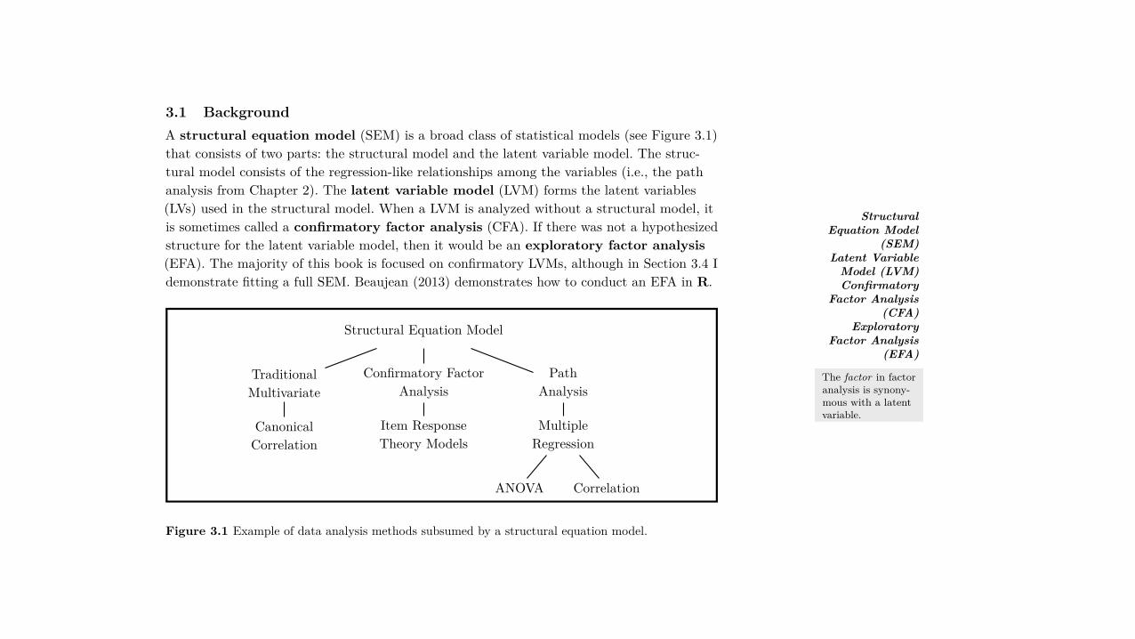
3.1 BackgroundA structural equation model (SEM) is a broad class of statistical models (see Figure 3.1)that consists of two parts: the structural model and the latent variable model. The struc-tural model consists of the regression-like relationships among the variables (i.e., the pathanalysis from Chapter 2). The latent variable model (LVM) forms the latent variables(LVs) used in the structural model. When a LVM is analyzed without a structural model, itis sometimes called a confirmatory factor analysis (CFA). If there was not a hypothesizedstructure for the latent variable model, then it would be an exploratory factor analysis(EFA). The majority of this book is focused on confirmatory LVMs, although in Section 3.4 Idemonstrate fitting a full SEM. Beaujean (2013) demonstrates how to conduct an EFA in R.
StructuralEquation Model
(SEM)Latent Variable
Model (LVM)Confirmatory
Factor Analysis(CFA)
ExploratoryFactor Analysis
(EFA)
The factor in factoranalysis is synony-mous with a latentvariable.
Structural Equation Model
TraditionalMultivariate
CanonicalCorrelation
Confirmatory FactorAnalysis
Item ResponseTheory Models
PathAnalysis
MultipleRegression
ANOVA Correlation
Figure 3.1 Example of data analysis methods subsumed by a structural equation model.
37
3 | Basic Latent Variable Models
Chapter Contents3.1 Background . . . . . . . . . . . . . . . . . . . . . . . . . . . . . . . . . . . . 373.2 Latent Variable Models . . . . . . . . . . . . . . . . . . . . . . . . . . . . . . 38
3.2.1 Identification of Latent Variable Models . . . . . . . . . . . . . . . . 393.3 Example: Latent Variable Model with One Latent Variable . . . . . . . . . . 42
3.3.1 Alternative Latent Variable Scaling . . . . . . . . . . . . . . . . . . . 473.3.2 Example: Latent Variable Model with Two Latent Variables . . . . . 48
3.4 Example: Structural Equation Model . . . . . . . . . . . . . . . . . . . . . . 503.5 Summary . . . . . . . . . . . . . . . . . . . . . . . . . . . . . . . . . . . . . . 513.6 Writing the Results . . . . . . . . . . . . . . . . . . . . . . . . . . . . . . . . 513.7 Exercises . . . . . . . . . . . . . . . . . . . . . . . . . . . . . . . . . . . . . . 523.8 References & Further Readings . . . . . . . . . . . . . . . . . . . . . . . . . . 55
3.1 BackgroundA structural equation model (SEM) is a broad class of statistical models (see Figure 3.1)that consists of two parts: the structural model and the latent variable model. The struc-tural model consists of the regression-like relationships among the variables (i.e., the pathanalysis from Chapter 2). The latent variable model (LVM) forms the latent variables(LVs) used in the structural model. When a LVM is analyzed without a structural model, itis sometimes called a confirmatory factor analysis (CFA). If there was not a hypothesizedstructure for the latent variable model, then it would be an exploratory factor analysis(EFA). The majority of this book is focused on confirmatory LVMs, although in Section 3.4 Idemonstrate fitting a full SEM. Beaujean (2013) demonstrates how to conduct an EFA in R.
StructuralEquation Model
(SEM)Latent Variable
Model (LVM)Confirmatory
Factor Analysis(CFA)
ExploratoryFactor Analysis
(EFA)
The factor in factoranalysis is synony-mous with a latentvariable.
Structural Equation Model
TraditionalMultivariate
CanonicalCorrelation
Confirmatory FactorAnalysis
Item ResponseTheory Models
PathAnalysis
MultipleRegression
ANOVA Correlation
Figure 3.1 Example of data analysis methods subsumed by a structural equation model.
37

X1
X2
X3
X4
Informação não redundante= " "#$% = & &#$
% =10
6 correlações e 4 variâncias

Y1
Y2
Y3
Y4
Informação não redundante= " "#$% = & &#$
% =106 correlações e 4 variâncias
Y1
Y2
Y3
Y4
X
4 cargas fatoriais e 4 variâncias de erro

38 Chapter 3. Basic Latent Variable Models
LV Var 2
Var 3
Var 1 E1
E2
E3
(a) LV is a reflective latent variable.
LVVar 2
Var 3
Var 1
ELV
(b) LV is a formative latent variable.
Figure 3.2 Reflective and formative latent variable path models.
Reflective andFormative LatentVariables
Indicator Variable
Factors are usedwith ANOVA mod-els, too. For the pur-poses of this book,consider that usageunrelated to its usewith LVMs.
Not all definitions ofa LV would includethe error term as alatent variable. SeeBollen (2002) formore about alterna-tive definitions.
g stands for generalintelligence.
Factor LoadingPatternCoe�cient
3.2 Latent Variable ModelsThere are two types of latent variables: reflective and formative. Reflective LVs are thoughtto cause other variables to covary, whereas formative LVs are thought to be the result of vari-ables’ covariation (similar to a regression model). Reflective and formative LVs are shown inFigure 3.2a and Figure 3.2b, respectively. I focus on reflective LVs in this book, although Igive some further reading on formative LVs in Section 3.8, and Exercise 3.3 requires the useof a formative LV.
The purpose of a (reflective) LVM is to understand the underlying structure that pro-duced relationships among multiple manifest variables (i.e., covariance matrix). The manifestvariables (MVs) that are directly influenced by the LV are the indicator variables. Theproposed causal agents in these underling structures are LVs. I first introduced latent vari-ables in Chapter 2 when discussing regression, as the error term is a latent variable: it isunobserved and influences a manifest variable (i.e., the outcome/endogenous variable); it ismeasured di�erently than typical LVs, though.
The idea behind a LVM is that there are a small number of LVs within a given domain(e.g., personality, self-e�cacy, religiosity) that influence each of its indicator variables and,hence, produce the observed covariances. Thus the variation (or covariation if there is morethan one) in the LVs causes (loosely defined) covariation in the indicators; conversely, covaria-tion in the indicator variables is due to their dependence on one or more LVs. Latent variablemodeling, then, is the method used to identify or confirm the number of the LVs that pro-duce the observed covariation in the indicator variables as well as understand the nature ofthose LVs (e.g., what they predict, what variables predict them).
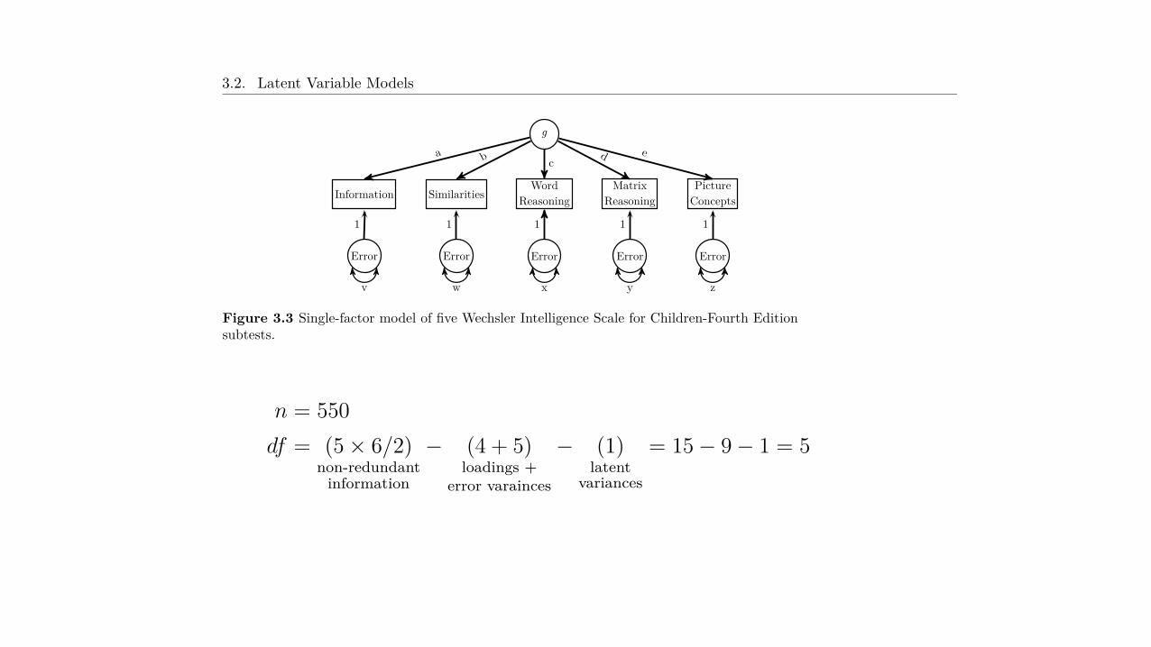
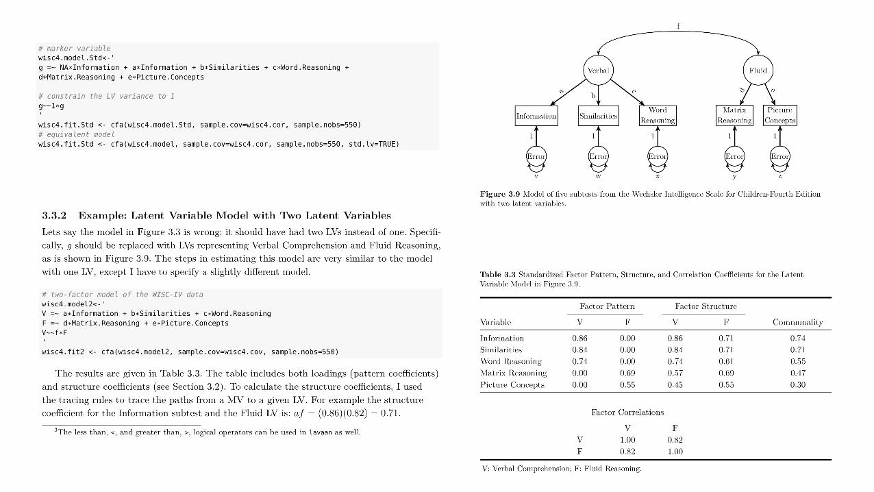
In path models, LVs are represented using ellipses. Figure 3.3 contains an example of aone-factor LVM using subtests from the Wechsler Intelligence Scale for Children-Fourth Edi-tion (WISC-IV; Wechsler, 2003). It has one LV, g, and five MVs, each of which is an indica-tor variable.
One measure of the influence a LV has on MVs is the factor loading. These are akin toregression/path coe�cients. Some scholars advocate using the term pattern coe�cient in-

Introduction to CFA 45
is more parsimonious than the measurement model because it attempts to reproduce the relationships among the latent variables with one less freely estimated parameter. Because of the overidentified nature of the structural portion of this model, its goodness of fit may be poorer than that of the measurement model. As illustrated by a tracing rule presented later in this chapter (e.g., Eq. 3.16), the structural portion of this model will result in poor fit if the product of the Factor X → Factor Z path and Factor Z → Factor Y path does not closely approximate the correlation between Factors X and Y estimated in the measurement model. Indeed, the indirect effects structural model in Figure 3.2B will be poor- fitting because the product of the X → Z and Z → Y direct effects [(.40)(.50) = .20] does not approximate the correlation between Factors X and Y (.60; see Figure 3.2A).
The purpose of this discussion is to illustrate that goodness of model fit is deter-mined by how adequately both the measurement and structural portions of a model are specified. A key aspect of CFA evaluation is the ability of the parameters from the mea-surement model (e.g., factor loadings and factor correlations) to reproduce the observed relationships among the indicators. If the CFA model is misspecified (e.g., failure to specify the correct number of factors, pattern of factor loadings), a poor- fitting solution will result. However, poor fit may also arise from a misspecified structural model which, like the model depicted in Figure 3.2B, often possesses fewer freely estimated param-eters than its corresponding measurement model. Because there are various potential sources of poor fit in CFA models involving multiple indicators, the researcher should establish a viable measurement model prior to pursuing a structural solution. If test-
FIGURE 3.2. Path diagrams of measurement and structural models.
Model A: Measurement Model
Model B: Structural Model

Conceitos práticos
§ EFA/ CFA Cargas fatoriais e comunalidade§ Pattern coefficients (corr parciais)
§ Structural coefficients (corr zero order)
§ Comunalidade e unicidade (R2)
§ Identificação§ Gl = info – parâmetros
§ Just-, under e over identified
§ Número de indicadores
§ Métrica da variável latente§ Padronizada (0/1), variável marcadora e
effect coding
Conceitos importantes

EFA vs CFA
38 CONFIRMATORY FACTOR ANALYSIS FOR APPLIED RESEARCH
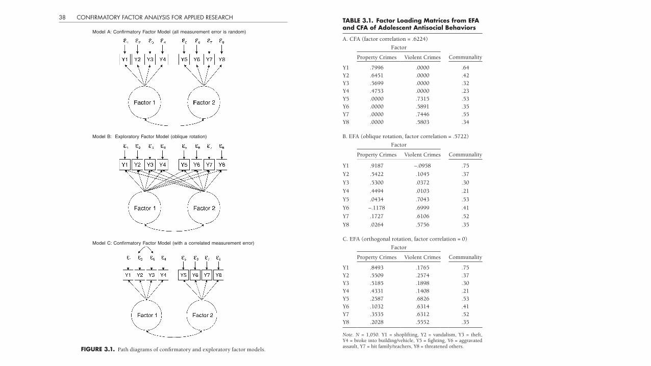
FIGURE 3.1. Path diagrams of confirmatory and exploratory factor models.
Model A: Confirmatory Factor Model (all measurement error is random)
Model B: Exploratory Factor Model (oblique rotation)
Model C: Confirmatory Factor Model (with a correlated measurement error)
Introduction to CFA 39
TABLE 3.1. Factor Loading Matrices from EFA and CFA of Adolescent Antisocial Behaviors
A. CFA (factor correlation = .6224)Factor
Property Crimes Violent Crimes Communality
Y1 .7996 .0000 .64Y2 .6451 .0000 .42Y3 .5699 .0000 .32Y4 .4753 .0000 .23Y5 .0000 .7315 .53Y6 .0000 .5891 .35Y7 .0000 .7446 .55Y8 .0000 .5803 .34
B. EFA (oblique rotation, factor correlation = .5722)Factor
Property Crimes Violent Crimes Communality
Y1 .9187 –.0958 .75Y2 .5422 .1045 .37Y3 .5300 .0372 .30Y4 .4494 .0103 .21Y5 .0434 .7043 .53Y6 –.1178 .6999 .41Y7 .1727 .6106 .52Y8 .0264 .5756 .35
C. EFA (orthogonal rotation, factor correlation = 0)Factor
Property Crimes Violent Crimes Communality
Y1 .8493 .1765 .75Y2 .5509 .2574 .37Y3 .5185 .1898 .30Y4 .4331 .1408 .21Y5 .2587 .6826 .53Y6 .1032 .6314 .41Y7 .3535 .6312 .52Y8 .2028 .5552 .35
Note. N = 1,050. Y1 = shoplifting, Y2 = vandalism, Y3 = theft, Y4 = broke into building/vehicle, Y5 = fighting, Y6 = aggravated assault, Y7 = hit family/teachers, Y8 = threatened others.

The Common Factor Model and EFA 25
ple size, number of indicators). The rationale of parallel analysis is that the factor should account for more variance than is expected by chance (as opposed to more variance than is associated with a given indicator, according to the logic of the Kaiser– Guttman rule). Using the 20- item data set, parallel analysis suggests four factors (see Figure 2.3). After the eigenvalue for the fourth factor, the eigenvalues from the randomly generated data (averages of 50 replications) exceed the eigenvalues of the research data. Although par-allel analysis frequently performs well, like the scree test it is sometimes associated with somewhat arbitrary outcomes (e.g., chance variation in the input correlation matrix may result in eigenvalues falling just above or below the parallel analysis criterion). A prac-tical drawback of the procedure is that it is not available in major statistical software packages such as SAS and SPSS, although parallel analysis is an option in the Mplus and Stata software programs, and in various shareware programs found on the Internet (e.g., O’Connor, 2001). In addition, Hayton, Allen, and Scarpello (2004) have provided syntax for conducting parallel analysis in SPSS, although the user must save and summarize the eigenvalues generated from random data outside of SPSS.
As noted above, when a factor estimation procedure other than ML is employed, eigenvalue- based procedures such as the Kaiser– Guttman rule, the scree test, and par-
FIGURE 2.3. Parallel analysis using eigenvalues from research and random data (average of 50 replications). Arrow indicates that eigenvalues from random data exceed the eigenvalues from research data after the fourth factor.
0
0.5
1
1.5
2
2.5
3
3.5
4
4.5
5
1 2 3 4 5 6 7 8 9 10 11 12 13 14 15 16 17 18 19 20Factor Number
Eig
enva
lue
Research Data
Random Data
30 CONFIRMATORY FACTOR ANALYSIS FOR APPLIED RESEARCH
FIGURE 2.4. Geometric representations of unrotated, orthogonally rotated, and obliquely rotated factor matrices.
A. Unrotated Factor Matrix
Factor
1 2
Y1 .834 –.160Y2 .813 –.099Y3 .788 –.088Y4 .642 .015Y5 .386 .329Y6 .333 .593Y7 .313 .497Y8 .284 .336
B. Orthogonally Rotated Factor Matrix (Varimax)
Factor
1 2
Y1 .836 .150Y2 .794 .199Y3 .767 .201Y4 .594 .244Y5 .242 .445Y6 .098 .673Y7 .114 .576Y8 .145 .416
C. Obliquely Rotated Factor Matrix (Promax)
Factor
1 2
Y1 .875 –.062Y2 .817 .003Y3 .788 .012Y4 .588 .106Y5 .154 .418Y6 –.059 .704Y7 –.018 .595Y8 .055 .413

16 CONFIRMATORY FACTOR ANALYSIS FOR APPLIED RESEARCH
stated earlier, unique variance is some combination of specific factor and measurement error variance. It is important to note that EFA and CFA do not provide separate esti-mates of specific variance and error variance.
In addition, Table 2.2 provides selected output from the Mplus program. As would be expected, many of the results are identical to those generated by SPSS (e.g., eigenval-ues, factor loadings). However, Mplus also provides other useful output, including an expanded set of goodness- of- fit statistics; standard errors and significance tests for the factor loadings (as well as for the residual variances, not shown in Table 2.2); and an estimate of factor determinacy (if requested by the user on the OUTPUT line; see Table 2.2). Each of these additional aspects of the Mplus output is discussed later in this book.
Path diagrams of the one- factor measurement model are provided in Figure 2.1. The first diagram presents the solution, using common symbols for the various elements of
FIGURE 2.1. Path diagram of the one- factor model.
1
Y4Y3Y2Y1
1 2 3 4
11 21 31 41
Depression
O4O3O2O1
.31 .29 .37 .44
.75.79.84.83
η
ε ε ε ε
λ λ λ λ
The Common Factor Model and EFA 17
factor models (and LISREL latent Y variable notation); the second diagram replaces these elements with the sample estimates obtained from the EFA presented in Table 2.1. Fol-lowing the conventions of factor analysis and structural equation modeling (SEM), the latent variable (factor) of Depression is depicted by a circle or an oval, whereas the four clinical ratings (indicators) are represented by squares or rectangles. The unidirectional arrows (→) represent the factor loadings (λ, or lambda), which are the regression slopes (direct effects) for predicting the indicators from the factor (η, or eta). These arrows are also used to relate the unique variances (ε, or epsilon) to the indicators.4
A fundamental equation of the common factor model is
yj = λj1η1 + λj2η2 + . . . + λjmηm + εj (2.1)
where yj represents the jth of p indicators (in the case p = 4; O1, O2, O3, O4) obtained from a sample of n independent participants (in this case, n = 300); λjm represents the factor loading relating variable j to the mth factor η (in the case m = 1; the single factor of Depression); and εj represents the variance that is unique to indicator yj and is indepen-dent of all ηs and all other εs. As will be seen in subsequent chapters, similar notation is used to represent some of the equations of CFA. In this simple factor solution entailing a single factor (η1) and four indicators, the regression functions depicted in Figure 2.1 can be summarized by four separate equations:
O1 = λ11η1 + ε1 (2.2) O2 = λ21η1 + ε2
O3 = λ31η1 + ε3
O4 = λ41η1 + ε4
This set of equations can be summarized in a single equation that expresses the relation-ships among observed variables (y), factors (η), and unique variances (ε):
y = Λyη + ε (2.3)
or in expanded matrix form:
Σ = ΛyΨΛ′y + Θε (2.4)
where Σ is the p × p symmetric correlation matrix of p indicators; Λy is the p × m matrix of factor loadings λ (in this case, a 4 × 1 vector); Ψ is the m × m symmetric correlation matrix of the factor correlations (1 × 1); and Θε is the p × p diagonal matrix of unique variances ε (p = 4). In accord with matrix algebra, matrices are represented in factor analysis and SEM by uppercase Greek letters (e.g., Λ, Ψ, and Θ), and specific elements of these matrices are denoted by lowercase Greek letters (e.g., λ, ψ, and ε). With minor variations, these fundamental equations can be used to calculate various aspects of the sample data from the factor analysis parameter estimates, such as the variances, covari-
EFA
18 CONFIRMATORY FACTOR ANALYSIS FOR APPLIED RESEARCH
ances, and means of the input indicators (the latter can be conducted in context of CFA with mean and covariance structures; see Chapter 7). For example, the following equa-tion reproduces the variance in the O1 indicator:
VAR(O1) = σ11 = λ112ψ11 + ε1 (2.5)
= .8282(1) + .315= 1.00
where ψ11 is the variance of the factor η1, and ε1 is the unique variance of O1. Note that both ψ11 and σ11 equal 1.00 because the EFA model is completely standardized; that is, when variables are standardized, their variances equal 1.00. Similarly, the model esti-mate of the covariance (correlation) of O1 and O2 can be obtained from the following equation:
COV(O1, O2) = σ21 = λ11ψ11λ21 (2.6)= (.828)(1)(.841)= .696
Because the solution is completely standardized, this covariance is interpreted as the factor model estimate of the sample correlation of O1 and O2. In other words, the model- implied correlation of the indicators is the product of their completely standardized fac-tor loadings. Note that the sample correlation of O1 and O2 is .70, which is very close to the factor- model- implied correlation of .696. As discussed in further detail in Chapter 3, the acceptability of factor analysis models is determined in large part by how well the parameter estimates of the factor solution (e.g., the factor loadings) are able to reproduce the observed relationships among the input variables. The current illustration should exemplify the point made earlier that common variance (i.e., variance explained by the factors as reflected by factor loadings and communalities) is estimated on the basis of the shared variance among the indicators used in the analysis. EFA generates a matrix of factor loadings (Λ) that best explain the correlations among the input indicators.
PROCEDURES OF EFA
Although a full description of EFA is beyond the scope of this book, an overview of its concepts and procedures is helpful to make later comparisons to CFA. The reader is referred to papers by Fabrigar, Wegener, MacCallum, and Strahan (1999); Floyd and Widaman (1995); and Preacher and MacCallum (2003) for detailed guidelines on con-ducting EFA in applied data sets.
As stated earlier, the overriding objective of EFA is to evaluate the dimensional-ity of a set of multiple indicators (e.g., items from a questionnaire) by uncovering the smallest number of interpretable factors needed to explain the correlations among them. Whereas the researcher must ultimately specify the number of factors, EFA is an “explor-

CFA

CFA
§ Modelos de medida. Ancorados na teoria§ Validade? Até que ponto os indicadores são medidas válidas doconstruto ?
§ Efeitos da variável latente?§ Até que ponto a variável latente é construto que se presume ?
§ Recurso para testar a dimensionalidade das medidas
§ Recurso para testar modelos alternativos§ Especifica-se dois modelos e verifica-se qual deles se ajusta melhoraos dados
§ Recurso para estimar correlações entre construtos não-atenuadas pelos erros de medida

Introduction Course Outline Notation Stats recap Latent Causes Estimation Conclusion

16 CONFIRMATORY FACTOR ANALYSIS FOR APPLIED RESEARCH
stated earlier, unique variance is some combination of specific factor and measurement error variance. It is important to note that EFA and CFA do not provide separate esti-mates of specific variance and error variance.
In addition, Table 2.2 provides selected output from the Mplus program. As would be expected, many of the results are identical to those generated by SPSS (e.g., eigenval-ues, factor loadings). However, Mplus also provides other useful output, including an expanded set of goodness- of- fit statistics; standard errors and significance tests for the factor loadings (as well as for the residual variances, not shown in Table 2.2); and an estimate of factor determinacy (if requested by the user on the OUTPUT line; see Table 2.2). Each of these additional aspects of the Mplus output is discussed later in this book.
Path diagrams of the one- factor measurement model are provided in Figure 2.1. The first diagram presents the solution, using common symbols for the various elements of
FIGURE 2.1. Path diagram of the one- factor model.
1
Y4Y3Y2Y1
1 2 3 4
11 21 31 41
Depression
O4O3O2O1
.31 .29 .37 .44
.75.79.84.83
η
ε ε ε ε
λ λ λ λ
48 CONFIRMATORY FACTOR ANALYSIS FOR APPLIED RESEARCH
error covariances, if any, in the off- diagonal. Less commonly, some notational systems do not use directional arrows in the depiction of error variances in order to avoid this potential source of confusion (one notational variation is to symbolize error variances with ovals because, like latent variables, measurement errors are not observed).
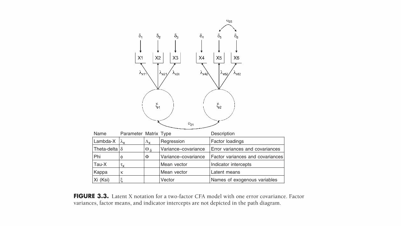
Factor variances and covariances are notated by phi (φ) and psi (ψ) in latent X and latent Y models, respectively. Curved, bidirectional arrows are used to symbolize covariances (correlations); in Figures 3.3 and 3.4, curved arrows indicate the covariance between the factors (φ21, ψ21) and the error covariance of the X5 and X6 indicators (δ65, ε65). When relationships are specified as covariances, the researcher is asserting that the variables are related (e.g., ξ1 and ξ2). However, this specification makes no claims about the nature of the relationship, due to either the lack of knowledge regarding the directionality of the association (e.g., ξ1 → ξ2) or the unavailability to the analysis of variables purported to account for this overlap (e.g., ξ1 and ξ2 are related because they share a common cause that is not represented by observed measures or latent variables in the analysis). Nonetheless, as discussed in Chapter 8, higher- order factor analysis is a useful approach for explaining the covariances among factors when a strong theory exists in regard to the patterning of the factor interrelationships.
The parameters in Figures 3.3 and 3.4 also possess numerical subscripts to indicate the specific elements of the relevant matrices. For example, λx11 (Figure 3.3) indicates
FIGURE 3.3. Latent X notation for a two- factor CFA model with one error covariance. Factor variances, factor means, and indicator intercepts are not depicted in the path diagram.
Name Parameter Matrix Type Description
Lambda-X λx Λx Regression Factor loadings
Theta-delta δ Θ δ Variance–covariance Error variances and covariances
Phi φ Φ Variance–covariance Factor variances and covariances
Tau-X τx Mean vector Indicator intercepts
Kappa κ Mean vector Latent means
Xi (Ksi) ξ Vector Names of exogenous variables
Introduction to CFA 49
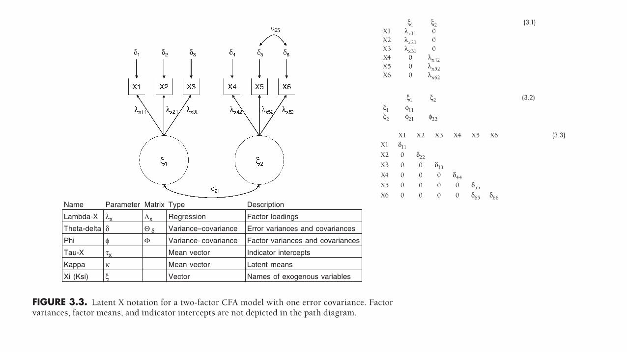
that the X1 measure loads on the first exogenous factor (ξ1), and λx21 indicates that X2 also loads on ξ1. This numeric notation assumes that the indicators are ordered X1, X2, X3, X4, X5, and X6 in the input variance– covariance matrix. If the input matrix is arranged in this fashion, the lambda X matrix (Λx) in Figure 3.3 will be as follows:
ξ1 ξ2 (3.1)X1 λx11 0X2 λx21 0X3 λx31 0X4 0 λx42X5 0 λx52X6 0 λx62
where the first numerical subscript refers to the row of Λx (i.e., the positional order of the X indicator), and the second numerical subscript refers to the column of Λx (i.e., the positional order of the exogenous factors, ξ). For example, λx52 conveys that the fifth indicator in the input matrix (X5) loads on the second latent X variable (ξ2). Thus Λx and Λy are full matrices whose dimensions are defined by p rows (number of indicators)
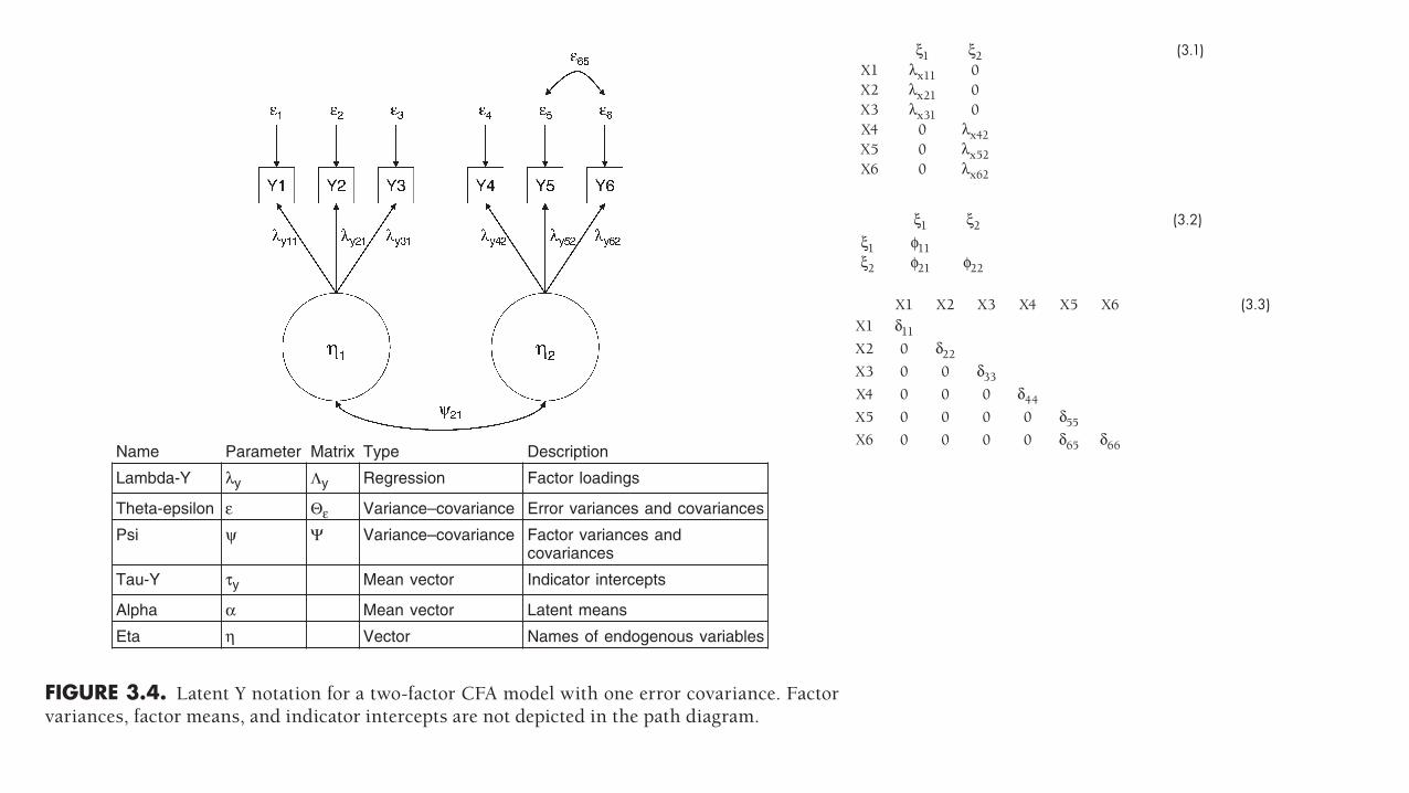
FIGURE 3.4. Latent Y notation for a two- factor CFA model with one error covariance. Factor variances, factor means, and indicator intercepts are not depicted in the path diagram.
Name Parameter Matrix Type Description
Lambda-Y λy Λy Regression Factor loadings
Theta-epsilon ε Θε Variance–covariance Error variances and covariances
Psi ψ Ψ Variance–covariance Factor variances andcovariances
Tau-Y τy Mean vector Indicator intercepts
Alpha α Mean vector Latent means
Eta η Vector Names of endogenous variables
Introduction to CFA 49
that the X1 measure loads on the first exogenous factor (ξ1), and λx21 indicates that X2 also loads on ξ1. This numeric notation assumes that the indicators are ordered X1, X2, X3, X4, X5, and X6 in the input variance– covariance matrix. If the input matrix is arranged in this fashion, the lambda X matrix (Λx) in Figure 3.3 will be as follows:
ξ1 ξ2 (3.1)X1 λx11 0X2 λx21 0X3 λx31 0X4 0 λx42X5 0 λx52X6 0 λx62
where the first numerical subscript refers to the row of Λx (i.e., the positional order of the X indicator), and the second numerical subscript refers to the column of Λx (i.e., the positional order of the exogenous factors, ξ). For example, λx52 conveys that the fifth indicator in the input matrix (X5) loads on the second latent X variable (ξ2). Thus Λx and Λy are full matrices whose dimensions are defined by p rows (number of indicators)
FIGURE 3.4. Latent Y notation for a two- factor CFA model with one error covariance. Factor variances, factor means, and indicator intercepts are not depicted in the path diagram.
Name Parameter Matrix Type Description
Lambda-Y λy Λy Regression Factor loadings
Theta-epsilon ε Θε Variance–covariance Error variances and covariances
Psi ψ Ψ Variance–covariance Factor variances andcovariances
Tau-Y τy Mean vector Indicator intercepts
Alpha α Mean vector Latent means
Eta η Vector Names of endogenous variables
50 CONFIRMATORY FACTOR ANALYSIS FOR APPLIED RESEARCH
and m columns (number of factors). The zero elements of Λx (e.g., λx12, λx41) indicate the absence of cross- loadings (e.g., the relationship between X1 and ξ2 is fixed to zero). This is also depicted in Figures 3.3 and 3.4 by the absence of directional arrows between certain indicators and factors (e.g., no arrow connecting ξ2 to X1 in Figure 3.3).
A similar system is used for variances and covariances among factors (φ in Figure 3.3, ψ in Figure 3.4) and indicator errors (δ and ε in Figures 3.3 and 3.4, respectively). However, because these aspects of the CFA solution reflect variances and covariances, they are represented by m × m symmetric matrices with variances on the diagonal and covariances in the off- diagonal. For example, the phi matrix (Φ) in Figure 3.3 will look as follows:
ξ1 ξ2 (3.2)ξ1 φ11ξ2 φ21 φ22
where φ11 and φ22 are the factor variances, and φ21 is the factor covariance. Similarly, the theta- delta matrix (Θδ) in Figure 3.3 is the following p × p symmetric matrix:
X1 X2 X3 X4 X5 X6 (3.3)X1 δ11
X2 0 δ22
X3 0 0 δ33
X4 0 0 0 δ44
X5 0 0 0 0 δ55
X6 0 0 0 0 δ65 δ66
where δ11 through δ66 are the indicator errors, and δ65 is the covariance of the mea-surement errors of indicators X5 and X6. For notational ease, the diagonal elements are indexed by single digits in Figures 3.3 and 3.4 (e.g., δ6 is the same as δ66). The zero ele-ments of Θδ (e.g., δ21) indicate the absence of error covariances (i.e., these relationships are fixed to zero).
In CFA with mean structures (see Chapter 7), indicator intercepts are symbolized by tau (τ), and latent exogenous and endogenous means are symbolized by kappa (κ) and alpha (α), respectively. Because the focus has been on CFA, only parameters germane to measurement models have been discussed thus far. LISREL notation also applies to structural component of models that entail directional relationships among exoge-nous and endogenous variables. For instance, gamma (γ, matrix: Γ) denotes regressions between latent X and latent Y variables, and beta (β, matrix: Β) symbolizes directional effects among endogenous variables. Most of the CFA illustrations provided in this book do not require gamma or beta parameters. Exceptions include CFA with covariates (e.g., MIMIC models, Chapter 7), where the measurement model is regressed on observed background measures (e.g., a dummy code indicating male versus female); higher- order CFA (Chapter 8); and models with formative indicators (Chapter 8).
48 CONFIRMATORY FACTOR ANALYSIS FOR APPLIED RESEARCH
error covariances, if any, in the off- diagonal. Less commonly, some notational systems do not use directional arrows in the depiction of error variances in order to avoid this potential source of confusion (one notational variation is to symbolize error variances with ovals because, like latent variables, measurement errors are not observed).
Factor variances and covariances are notated by phi (φ) and psi (ψ) in latent X and latent Y models, respectively. Curved, bidirectional arrows are used to symbolize covariances (correlations); in Figures 3.3 and 3.4, curved arrows indicate the covariance between the factors (φ21, ψ21) and the error covariance of the X5 and X6 indicators (δ65, ε65). When relationships are specified as covariances, the researcher is asserting that the variables are related (e.g., ξ1 and ξ2). However, this specification makes no claims about the nature of the relationship, due to either the lack of knowledge regarding the directionality of the association (e.g., ξ1 → ξ2) or the unavailability to the analysis of variables purported to account for this overlap (e.g., ξ1 and ξ2 are related because they share a common cause that is not represented by observed measures or latent variables in the analysis). Nonetheless, as discussed in Chapter 8, higher- order factor analysis is a useful approach for explaining the covariances among factors when a strong theory exists in regard to the patterning of the factor interrelationships.
The parameters in Figures 3.3 and 3.4 also possess numerical subscripts to indicate the specific elements of the relevant matrices. For example, λx11 (Figure 3.3) indicates
FIGURE 3.3. Latent X notation for a two- factor CFA model with one error covariance. Factor variances, factor means, and indicator intercepts are not depicted in the path diagram.
Name Parameter Matrix Type Description
Lambda-X λx Λx Regression Factor loadings
Theta-delta δ Θ δ Variance–covariance Error variances and covariances
Phi φ Φ Variance–covariance Factor variances and covariances
Tau-X τx Mean vector Indicator intercepts
Kappa κ Mean vector Latent means
Xi (Ksi) ξ Vector Names of exogenous variables

Identificação e definição da métrica
40 Chapter 3. Basic Latent Variable Models
X1
X2
X3
X1
‡2
1
X2
‡12
‡2
2
X3
‡13
‡23
‡2
3
(a) Covariance matrix showing non-redundantelements.
LV
X2 X3X1
E1 E2 E3
a bc
1 1 1
d e f
(b) Latent variable model.
Figure 3.4 Example with three indicator variables.
Degrees ofFreedom
For factor and pathanalysis, identifi-cation is relativelysimple to determine.Most of the di�cultywith identification iswith full SEMs.
fied. Conversely, if there are more pieces of non-redundant information than there are param-eters to estimate, then the model is usually overidentified. If a model is underidentified, themodel’s parameters cannot be estimated uniquely and lavaan (or any other LVM program)will return an error message. If a model is over- or just-identified, there should be uniqueestimates for each parameter. For overidentified models, not only do they provide unique pa-rameter estimates, but they can also provide measures of model fit (see Appendix A). Thisis because they have degrees of freedom (df ). In LVMs, df can be thought of as the num-ber of non-redundant pieces of information in the data minus the number of parameters toestimate. Only overidentified models have df > 0.
Model identification can be tricky. Instead of going into all the complexities involved,I give four rules-of-thumb conditions in the next three sections that should work for mostmodels with reflective LVs. Meeting these conditions typically produces an overidentifiedLVM, or at least a just-identified LVM.
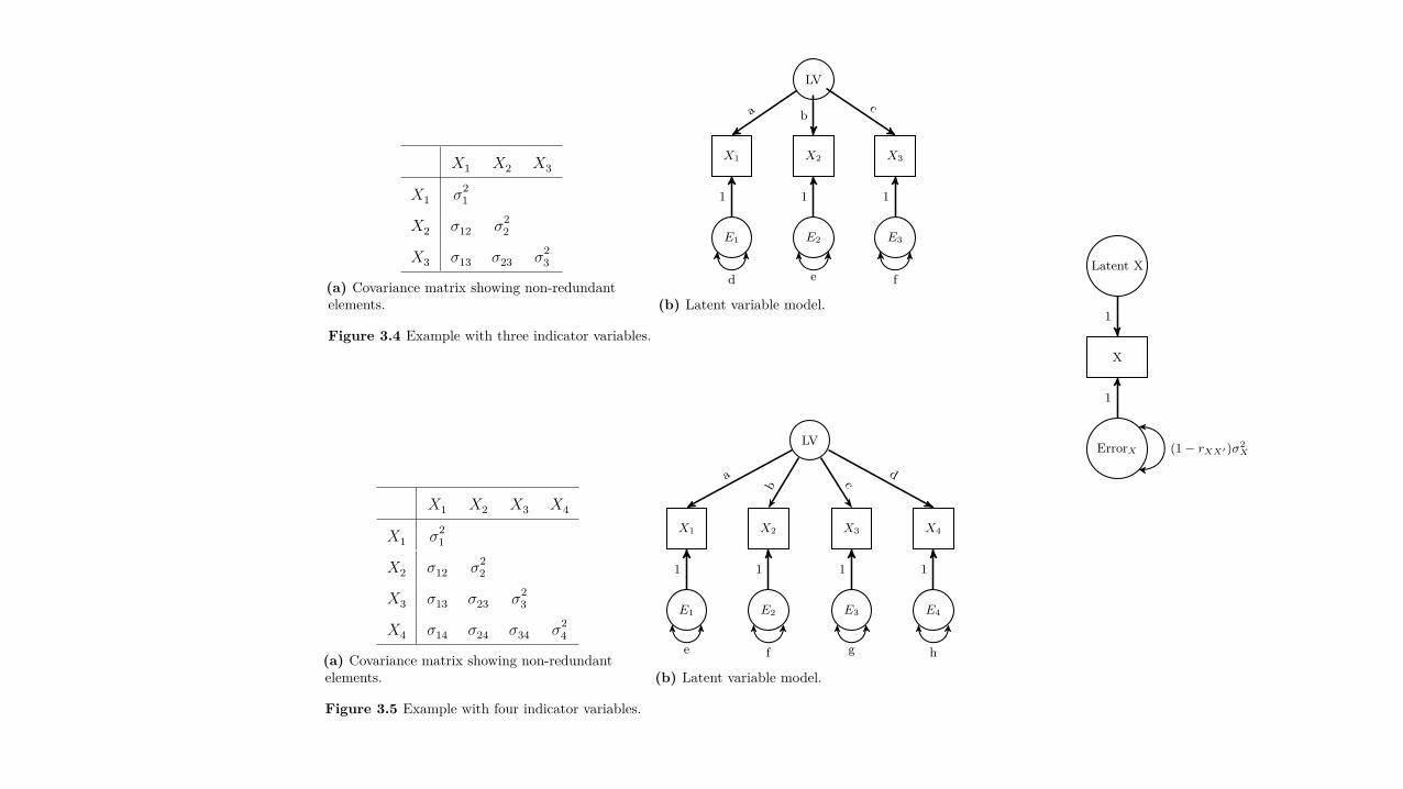
3.2.1.1 Number of Indicator VariablesIf every latent variable in a model has at least four indicator variables and none of their errorvariances covary, then there should not be a problem with identification. Why four variables?,you may ask. Examine Figure 3.4 where there are 3 ◊ 4/2 = 6 pieces of non-redundant informa-tion, and 6 parameters to estimate. Thus, it is just-identified. Now examine Figure 3.5, wherethere are 4 ◊ 5/2 = 10 pieces of non-redundant information, but only 8 parameters to estimate,making it overidentified.
Even if a LV cannot have at least four indicators, it can still be just-identified under anyof the following conditions.
1. The LV has three indicator variables, and the error variances do not covary.2. The LV has at least two indicators with non-covarying error variances and the indica-
tor variables’ loadings are set equal to each other.3. The LV has one indicator, the directional paths are set to one, and its error variance is
fixed to some value. The fixed value is usually either:
3.2. Latent Variable Models 41
(a) 0.0, meaning the indicator variable is measured with perfect reliability, or(b) (1 ≠ rXXÕ)‡
2
X , where rXXÕ and ‡2
X are the variable’s reliability and variance,respectively.
An example of a single-indicator LVM is shown in Figure 3.6.
3.2.1.2 Latent Variable’s ScaleBecause LVs are not directly observed, there are no inherent units by which to measurethem.Consequently, a LVM is not identified unless some parameter estimates are constrainedto set the latent variable’s scale. There are three common ways to set this scale.
1. Standardized latent variable. This method constrains the latent variable’s variance to1.0. This, in e�ect, makes the latent variable a standardized variable (i.e, on a Z scorescale; see Section 1.1.12.2). If the indicator variables are standardized as well, the load-ings can be interpreted the same as a standardized regression coe�cient: the numberof standard deviations the MV changes as the LV increases one standard deviation.Moreover, if there is more than one LV, then the covariance among the LVs becomes acorrelation.
2. Marker variable. This method requires a single factor loading for each LV be con-strained to an arbitrary value (usually 1.0). The indicator variable whose loading isconstrained is called the marker variable. This method uses the marker variable to de-fine the LV’s variance.
3. E�ects-coding. This method estimates all the loadings, but constrains that the loadingsfor a given LV average 1.0, or, equivalently, that their sum is equal to the number ofunique indicator variables.
These di�erent scaling methods produce di�erent values for the model’s parameters, butshould not alter how a model fits the data. I demonstrate all three scaling methods in Sec-tion 3.3.1.
X1
X2
X3
X4
X1
‡2
1
X2
‡12
‡2
2
X3
‡13
‡23
‡2
3
X4
‡14
‡24
‡34
‡2
4
(a) Covariance matrix showing non-redundantelements.
LV
X2X1 X3 X4
E1 E2 E3 E4
a
b c d
1 1 1 1
e f g h
(b) Latent variable model.
Figure 3.5 Example with four indicator variables.
42 Chapter 3. Basic Latent Variable Models
Figure 3.6 Example of a latent variablemodel with a single indicator.
Latent X
X
ErrorX
1
1
(1 ≠ rXXÕ )‡2X
EmpiricalUnderidentification
3.2.1.3 Other ConditionsThere are two other conditions for the rules-of-thumb. It is atypical for these conditions notto be met, so I do not discuss them in any detail.
1. If there is more than one LV in the model, then for every pair of LVs, either:(a) There is at least one indicator variable per LV whose error variance does not
covary with the error variance of the other LV’s indicator variables, or(b) The covariance between the pair of LVs is constrained to a specified value.
2. For every indicator variable, there must be at least one other indicator variable (of thesame LV or a di�erent LV) with whom the error variances do not covary.
3.2.1.4 Empirical UnderidentificationEmpirical underidentification is the situation where a LVM is only identified if one ofthe parameters (usually a factor correlation or a factor loading) is not equal, or very closeto, 0.0.1 An example is shown in Figure 3.7. As long as |e| > 0, the model in Figure 3.7ais overidentified because there are 4 ◊ 5/2 = 10 pieces of information with 9 parametersto estimate. However if e = 0, then the model requires the estimation of two separate LVs,as is the case in Figure 3.7b. For both LVs, there are 2 ◊ 3/2 = 3 pieces of non-redundantinformation, but 4 parameters to estimate, making them each underidentified.
3.3 Example: Latent Variable Model with One Latent VariableI demonstrate fitting a LVM in R by estimating the parameters for the model in Figure 3.3using the data in Table 3.1. My syntax to enter the correlations and standard deviations(SDs) is given below.
library(lavaan)# convert vector of correlations into matrixwisc4.cor <- lower2full(c(1,0.72,1,0.64,0.63,1,0.51,0.48,0.37,1,0.37,0.38,0.38,0.38,1))# name the variables in the matrixcolnames(wisc4.cor) <- rownames(wisc4.cor) <- c("Information", "Similarities","Word.Reasoning", "Matrix.Reasoning", "Picture.Concepts")
1Sometimes the issue of empirical underidentification can arise if factor correlations are very close to 1.0 aswell.
3.2. Latent Variable Models 39
g
WordReasoningSimilaritiesInformation
MatrixReasoning
PictureConcepts
Error Error Error Error Error
a b cd e
1 1 1 1 1
v w x y z
Figure 3.3 Single-factor model of five Wechsler Intelligence Scale for Children-Fourth Editionsubtests.
stead of factor loading because factor loading is an ambiguous term that can be confusedwith structure coe�cient, which are the correlations between the MVs and the model’sLVs. For models with one LV, pattern and structure coe�cients have the same values. Formodels with more than one LV (see Section 3.3.2), they have di�erent values unless all theLVs are uncorrelated with each other. To minimize confusion in this book, when I use theterms factor loading or loading, I am referring to a pattern coe�cient. When I discuss struc-ture coe�cients, I use the term explicitly.
In Figure 3.3, a, b, c, d, and e are all factor loadings. I can obtain something akin to a R2
value for each MV using the tracing rules discussed in Section 2.1.3: find all the legitimatepaths that go from a MV to the LV(s) and return back to the same MV. This value is calledthe communality. Conversely, the uniqueness is the amount of variance in the MV notexplained by the model’s LVs. For example, to find the communality for the Information MVin Figure 3.3, I can go to the LV, g, and then back to Information only through the a path(twice), thus the amount of variance of the Information MV that g explains is a
2. This makesuniqueness of the Information variable: 1 ≠ a
2
= v.
3.2.1 Identification of Latent Variable ModelsAt the heart of model identification is the question: Is there enough non-redundant infor-
mation in the data to be able to estimate the required parameters uniquely? With regression,identification is never an issue because they are always just-identified models, meaning thatthe number of parameters to estimate exactly equals the amount of non-redundant informa-tion in the data. For now, think of the amount of non-redundant information in the data asbeing the number of non-redundant variances/covariances in the dataset. This can be easilycalculated using the formula in Equation (3.1).
non-redundant information in a dataset =
p(p + 1)
2
(3.1)
where p is the number of manifest variables.
With a LVM, model identification is more complex than with regression, as the modelscan be just-identified, underidentified, or overidentified. If there are more parameters toestimate than there are pieces of non-redundant information, then the model is underidenti-
StructureCoe�cient
Communality
Uniqueness
Identification ofLatent Variable
Just-IdentifiedModel
UnderidentifiedModel
OveridentifiedModel
3.3. Example: Latent Variable Model with One Latent Variable 45
g
WordReasoningSimilaritiesInformation
MatrixReasoning
PictureConcepts
Error Error Error Error Error
0.860.8
4 0.740.58
0.47
1 1 1 1 1
0.26 0.3 0.45 0.67 0.78
1
Figure 3.8 Single-factor model of five Wechsler Intelligence Scale for Children-Fourth Editionsubtests with standardized parameter estimates.
## 2 g =~ Similarities b 0.98 0.045 2.5 0.84 0.84## 3 g =~ Word.Reasoning c 0.86 0.045 2.2 0.74 0.74## 4 g =~ Matrix.Reasoning d 0.65 0.047 1.7 0.58 0.58## 5 g =~ Picture.Concepts e 0.54 0.050 1.4 0.47 0.47## 6 Information ~~ Information 2.40 0.250 2.4 0.27 0.27## 7 Similarities ~~ Similarities 2.71 0.258 2.7 0.30 0.30## 8 Word.Reasoning ~~ Word.Reasoning 4.01 0.295 4.0 0.45 0.45## 9 Matrix.Reasoning ~~ Matrix.Reasoning 5.55 0.360 5.6 0.67 0.67## 10 Picture.Concepts ~~ Picture.Concepts 6.91 0.434 6.9 0.78 0.78## 11 g ~~ g 6.65 0.564 1.0 1.00 1.00
The top part of lavaan’s summary() output can be used to double-check to make sure themodel was specified correctly. For this model:
n = 550
df = (5 ◊ 6/2)
non-redundant
information
≠ (4 + 5)
loadings +
error varainces
≠ (1)
latent
variances
= 15 ≠ 9 ≠ 1 = 5
both of which are correct. The Latent variables section of the output gives the unstandard-ized and standardized parameter estimates (in this example, they are all loadings), both ofwhich indicate that each indicator is a relatively strong measure of g, with Information beingthe most saturated (i.e., having the strongest loading) and Picture Concepts being the least.The Variances section gives the variances of the exogenous variables and the error variancesof the endogenous variables. A path model with all the standardized parameter estimates isshown in Figure 3.8.
lavaan does not produce communality estimates, but I can calculate them using the trac-ing rules. For example, the communality estimate for the Information subtest is a ◊ 1 ◊ a =
a2
= 0.86
2
= 0.74, thus its uniqueness is 1 ≠ a2
= 1 ≠ 0.86
2
= 0.26. Table 3.2 shows the factorloadings and communality estimates for all the indicator variables.
56 CONFIRMATORY FACTOR ANALYSIS FOR APPLIED RESEARCH
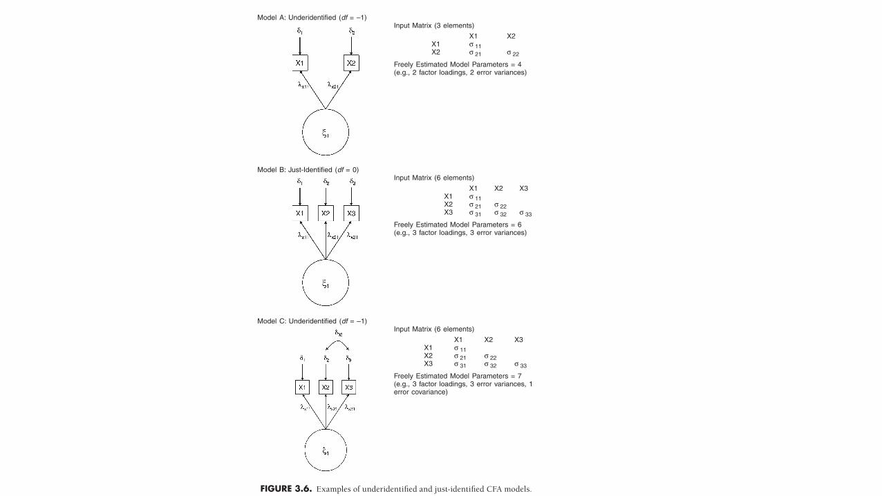
FIGURE 3.6. Examples of underidentified and just- identified CFA models.
Model A: Underidentified (df = –1)Input Matrix (3 elements)
X1 X2X1 σ 11X2 σ 21 σ 22
Freely Estimated Model Parameters = 4(e.g., 2 factor loadings, 2 error variances)
Model B: Just-Identified (df = 0)Input Matrix (6 elements)
X1 X2 X3X1 σ 11X2 σ 21 σ 22X3 σ 31 σ 32 σ 33
Freely Estimated Model Parameters = 6(e.g., 3 factor loadings, 3 error variances)
Model C: Underidentified (df = –1)Input Matrix (6 elements)
X1 X2 X3X1 σ 11X2 σ 21 σ 22X3 σ 31 σ 32 σ 33
Freely Estimated Model Parameters = 7(e.g., 3 factor loadings, 3 error variances, 1error covariance)
Introduction to CFA 51
FUNDAMENTAL EQUATIONS OF A CFA MODEL
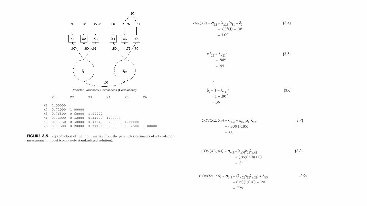
CFA aims to reproduce the sample variance– covariance matrix by the parameter esti-mates of the measurement solution (e.g., factor loadings, factor covariances, etc.). To illustrate, Figure 3.3 has been revised: Parameter estimates have been inserted for all factor loadings, factor correlation, and indicator errors (see now Figure 3.5). For ease of illustration, completely standardized values are presented, although the same concepts and formulas apply to unstandardized solutions. The first three measures (X1, X2, X3) are indicators of one latent construct (ξ1), whereas the next three measures (X4, X5, X6) are indicators of another latent construct (ξ2). It can be said, for example, that indicators X4, X5, and X6 are congeneric (cf. Jöreskog, 1971a) because they share a common factor (ξ2).5 An indicator is not considered congeneric if it loads on more than one factor.
In the case of congeneric factor loadings, the variance of an indicator is reproduced by multiplying its squared factor loading by the variance of the factor, and then sum-ming this product with the indicator’s error variance. The predicted covariance of two indicators that load on the same factor is computed as the product of their factor load-ings times the variance of the factor. The model- implied covariance of two indicators
FIGURE 3.5. Reproduction of the input matrix from the parameter estimates of a two- factor measurement model (completely standardized solution).
Predicted Variances–Covariances (Correlations):
X1 X2 X3 X4 X5 X6
X1 1.00000X2 0.72000 1.00000X3 0.76500 0.68000 1.00000X4 0.36000 0.32000 0.34000 1.00000X5 0.33750 0.30000 0.31875 0.60000 1.00000X6 0.31500 0.28000 0.29750 0.56000 0.72500 1.00000
52 CONFIRMATORY FACTOR ANALYSIS FOR APPLIED RESEARCH
that load on separate factors is estimated as the product of their factor loadings times the factor covariance. For example, based on the parameter estimates in the solution presented in Figure 3.5, the variance of X2 can be reproduced by the following equation (using latent X notation):
VAR(X2) = σ22 = λx212φ11 + δ2 (3.4)
= .802(1) + .36
= 1.00
In the case of completely standardized solutions (such as the current illustration), one can reproduce the variance of an indicator by simply squaring its factor loading (.802) and adding its error (.36), because the factor variance will always equal 1.00 (how-ever, the factor variance must be included in this calculation when one is dealing with unstandardized solutions). Note that the variance of ξ2 also equals 1.00 because of the completely standardized model (e.g., variance of X6 = λx62
2φ22 + δ6 = .702 + .51 = 1.00).The squared factor loading represents the proportion of variance in the indicator
that is explained by the factor (often referred to as a communality; see Chapter 2). For example, the communality of X2 is
η222 = λx21
2 (3.5)= .802
= .64
indicating that ξ1 accounts for 64% of the variance in X2. Similarly, in the completely standardized solution presented in Figure 3.5, the errors represent the proportion of variance in the indicators that is not explained by the factor; for example, δ2 = .36, indicating that 36% of the variance in X2 is unique variance (e.g., measurement error). These errors (residual variances) can be readily calculated as 1 minus the squared factor loading. Using the X2 indicator, the computation is:
δ2 = 1 – λx212 (3.6)
= 1 – .802
= .36
The predicted covariance (correlation) between X2 and X3 is estimated as follows:
COV(X2, X3) = σ3,2 = λx21φ11λx31 (3.7)= (.80)(1)(.85)
= .68
As before, in the case of completely standardized solutions the factor variance will always equal 1.00, so the predicted correlation between two congeneric indicators can
Introduction to CFA 53
be calculated by the product of their factor loadings; for instance, model- implied cor-relation of X4, X5 = .80(.75) = .60.
The predicted covariance (correlation) between X3 and X4 (indicators that load on separate factors) is estimated as follows:
COV(X3, X4) = σ4,3 = λx31φ21λx42 (3.8)= (.85)(.50)(.80)
= .34
Note that the factor correlation (φ21) rather than the factor variance is used in this cal-culation.
Figure 3.5 presents the 6 variances and 15 covariances (completely standardized) that are estimated by the two- factor measurement model. This model also contains a correlation between the errors of the X5 and X6 indicators (δ65 = .20). In this instance, the covariation between the indicators is not accounted for fully by the factor (ξ2); that is, X5 and X6 share additional variance due to influences other than the latent construct (e.g., method effects). Thus the equation to calculate the predicted correlation of X5 and X6 includes the correlated error:
COV(X5, X6) = σ6,5 = (λx52φ22λx62) + δ65 (3.9)= (.75)(1)(.70) + .20
= .725
CFA MODEL IDENTIFICATION
In order to estimate the parameters in CFA, the measurement model must be identi-fied. A model is identified if, on the basis of known information (i.e., the variances and covariances in the sample input matrix), it is possible to obtain a unique set of parameter estimates for each parameter in the model whose values are unknown (e.g., factor load-ings, factor correlations). Model identification pertains in part to the difference between the number of freely estimated model parameters and the number of pieces of informa-tion in the input variance– covariance matrix. Before this issue is addressed, an aspect of identification specific to the analysis of latent variables is discussed— scaling the latent variable.
Scaling the Latent Variable
In order for a researcher to conduct a CFA, every latent variable must have its scale identified. By nature, latent variables are unobserved and thus have no defined metrics (units of measurement). Thus these units of measurement must be set by the researcher. In CFA, this is most often accomplished in one of two ways.
54 CONFIRMATORY FACTOR ANALYSIS FOR APPLIED RESEARCH
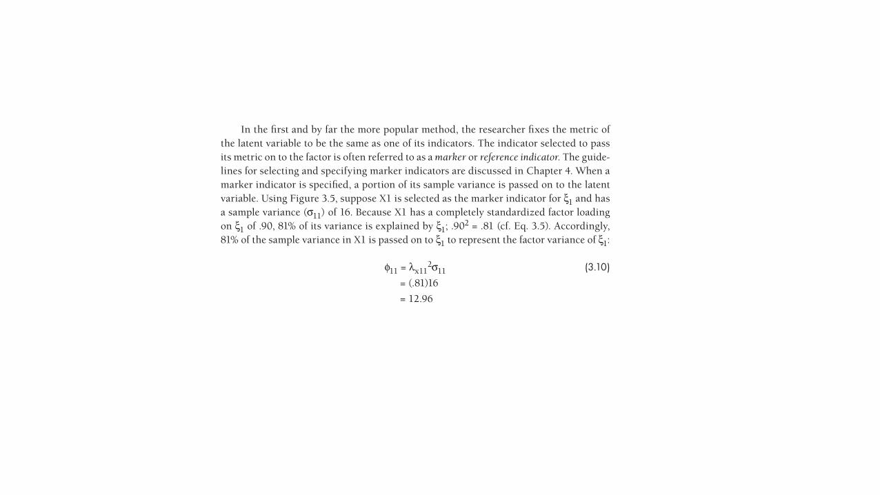
In the first and by far the more popular method, the researcher fixes the metric of the latent variable to be the same as one of its indicators. The indicator selected to pass its metric on to the factor is often referred to as a marker or reference indicator. The guide-lines for selecting and specifying marker indicators are discussed in Chapter 4. When a marker indicator is specified, a portion of its sample variance is passed on to the latent variable. Using Figure 3.5, suppose X1 is selected as the marker indicator for ξ1 and has a sample variance (σ11) of 16. Because X1 has a completely standardized factor loading on ξ1 of .90, 81% of its variance is explained by ξ1; .902 = .81 (cf. Eq. 3.5). Accordingly, 81% of the sample variance in X1 is passed on to ξ1 to represent the factor variance of ξ1:
φ11 = λx112σ11 (3.10)
= (.81)16
= 12.96
As will be shown in Chapter 4, these estimates are part of the unstandardized CFA solu-tion.
In the second method, the variance of the latent variable is fixed to a specific value, usually 1.00. Consequently, a standardized and a completely standardized solution are produced. Although the latent variables have been standardized (i.e., their variances are fixed to 1.00), the fit of this model is identical to that of the unstandardized model (i.e., models estimated using marker indicators). While it is useful in some circumstances (e.g., as a parallel to the traditional EFA model), this method is used less often than the marker indicator approach. The former strategy produces an unstandardized solution (in addition to a completely standardized solution), which is useful for several purposes, such as tests of measurement invariance across groups (Chapter 7) and evaluations of scale reliability (Chapter 8). However, in many instances this method of scale setting can be considered superior to the marker indicator approach, especially when the indicators have been assessed on an arbitrary metric, and when the completely standardized solu-tion is of more interest to the researcher (coupled with the fact that some programs, like Mplus, now provide standard errors and significance tests for standardized parameter estimates).
More recently, Little, Slegers, and Card (2006) have introduced a third method of scaling latent variables that is akin to effects coding in ANOVA. In this approach, a priori constraints are placed on the solution, such that the set of factor loadings for a given construct average to 1.00 and the corresponding indicator intercepts sum to zero. Consequently, the variance of the latent variables reflects the average of the indicators’ variances explained by the construct, and the mean of the latent variable is the opti-mally weighted average of the means for the indicators of that construct. Thus, unlike the marker indicator approach— where the variances and means of the latent variables will vary, depending on which indicator is selected as the marker indicator— the method developed by Little et al. (2006) has been termed nonarbitrary because the latent vari-able will have the same unstandardized metric as the average of all its manifest indica-tors. This approach is demonstrated in Chapter 7.

Exercício 5 § http://www.labape.com.br/rprimi/SEM/exerc18/Ex5.html

Índices de Ajuste

!2

SRMR

RMSEA

CFITLI

Generalguidelines
§ SRMR <=.08
§ RMSEA <=.06 (.08)
§ CFI e TLI >=.95 (.90)
92 CORE TECHNIQUES
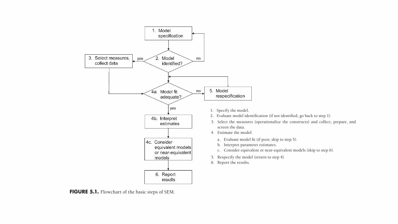
3. Select the measures (operationalize the constructs) and collect, prepare, and screen the data.
4. Estimate the model:
a. Evaluate model fit (if poor, skip to step 5).b. Interpret parameter estimates.c. Consider equivalent or near-equivalent models (skip to step 6).
5. Respecify the model (return to step 4).6. Report the results.
Specification
The representation of your hypotheses in the form of a structural equation model is specification. Many researchers begin the process of specification by drawing a model diagram using a set of more or less standard graphical symbols (defined later), but the model can alternatively be described by a series of equations. These equations define the model’s parameters, which correspond to presumed relations among observed or
FIGURE 5.1. Flowchart of the basic steps of SEM.
91
5
Specification
The specification of path analysis (PA) models, confirmatory factor analysis (CFA) mea-surement models, and structural regression (SR) models is the topic of this chapter. Out-lined first are the basic steps of SEM and graphical symbols used in model diagrams. Some straightforward rules are suggested for counting the number of observations (which is not the sample size) in the analysis and the number of model parameters. Both of these quantities are needed for checking model identification (next chapter). Actual research examples dealt with in more detail in later chapters are also intro-duced. The main goal of this presentation is to give you a better sense of the kinds of hypotheses that can be tested with core structural equation models.
STEPS OF SEM
Six basic steps are followed in most analyses, and two additional optional steps, in a per-fect world, would be carried out in every analysis. Review of these steps will help you to understand (1) the relation of specification, the main topic of this chapter, to later steps of SEM and (2) the utmost importance of specification.
Basic Steps
The basic steps are listed next and then discussed afterward, and a flowchart of these steps is presented in Figure 5.1. These steps are actually iterative because problems at a later step may require a return to an earlier step. (Later chapters elaborate specific issues at each step beyond specification for particular SEM techniques.)
1. Specify the model.2. Evaluate model identification (if not identified, go back to step 1).
92 CORE TECHNIQUES
3. Select the measures (operationalize the constructs) and collect, prepare, and screen the data.
4. Estimate the model:
a. Evaluate model fit (if poor, skip to step 5).b. Interpret parameter estimates.c. Consider equivalent or near-equivalent models (skip to step 6).
5. Respecify the model (return to step 4).6. Report the results.
Specification
The representation of your hypotheses in the form of a structural equation model is specification. Many researchers begin the process of specification by drawing a model diagram using a set of more or less standard graphical symbols (defined later), but the model can alternatively be described by a series of equations. These equations define the model’s parameters, which correspond to presumed relations among observed or
FIGURE 5.1. Flowchart of the basic steps of SEM.