An Updated F RTRAN-77 Version of the 2-D Static Neutron ...

KfK 4133 Juni1987

An Updated F RTRAN-77 Version of the 2-D Static Neutron

Transpo- Code Diamant 2 for Regular riangular eomet

K. Küfner, J. Burkhard, R. Heger Institut für Neutronenphysik und Reaktortechnik

\ Projekt Schneller Brüter

Kernforschungszentrum Karlsruhe

KERNFORSCHUNGSZENTRUM KARLSRUHE

Institut für Neutronenphysik und Reaktortechnik Projekt Schneller Brüter

KfK 4133

AN UPDATED FORTRAN-77 VERSION OF THE 2-D STATIC NEUTRON TRANSPORT CODE

DIAMANT2 FOR REGULAR TRIANGULAR GEOMETRY

Klaus Küfner, Jürgen Burkhard; Renate Heger

Kernforschungszentrum Karlsruhe GmbH, Karlsruhe

Als Manuskript vervielfältigt Für diesen Bericht behalten wir uns alle Rechte vor

Kernforschungszentrum Karlsruhe GmbH Postfach 3640, 7500 Karlsruhe 1

ISSN 0303-4003

ABSTRACT

This report describes a major revision of the DIAMANT2 code, which evolved

from the DIAMANT-code. DIAMANT2 solves the static multigroup neutron trans

port equation in planar geometry using the SN-method. Spatial discretization

is accomplished by taking finite differences on a meshgrid composed of

equilateral triangles. This new version of DIAMANT2 is written in FORTRAN77

and designed to run on scalar and vector computers. This report contains a

detailed documentation of the program and the input description as well as

some experiences gained with the code on several vector computers.

EINE ÜBERARBEITETE FORTRAN-77 VERSION DES 2-D NEUTRONEN

TRANSPORT PROGRAMMES DIAMANT2 FÜR REGULÄRE DREIECKSGEOMETRIE

ZUSAMMEN FASSUNG

Der Bericht beschreibt eine gründlich überarbeitete Version des DIM1ANT2

Programms, das aus dem DIAMANT Programm entstand. DIAMANT2 löst die

stationäre Multigruppen-Neutronen-Transport··Gleichung in ebener Geometrie

mit Hilfe der SN-Methode. Die räumliche Diskretisierung erfolgt über einem

Gitter aus gleichseitigen Dreiecken. Diese neue Version von DIAMANT2 ist in

FORTRAN-77 geschrieben und wurde speziell angelegt, um sowohl auf Skalar

als auch auf Vektorrechnern zu laufen. Der Bericht enthält eine ausführliche

Programmdokumentation und die Eingabebeschreibung sowie Erfahrungen mit dem

Einsatz des Codes auf mehreren Vektorrechnern.

Abstract iii

iv DIAMANT2 - Version 2.0

TABLE OF CONTENTS

Chapter 1. I ntroduction ••••••••••• fl ••• " •••••••

Chapter 2. Difference Equations and Solution Algorithm

2.1 Analytic Form of the Static Neutron Transport Equation

2.1 .1 Divergence Operator

2.1 .2 Spherical Harmonics Expansion of the Scattering Source Terms

2.2 Multigroup Equations

2.3 Discrete Ordinates Approach

2.3.1 SN-Constants and Angular Grientation

2.3.2 Construction of SN-Constants

2.3.3 Boundary Conditions ....

2.3.3.1 Vacuum Boundary Condition

2.3.3.2 Reflective Boundary Conditions

2.3.3.3 Boundary Fluxes

2.4 Difference Equations

2.5 Inner Iterations

2.5.1

2.5.2

2.5.3

2.5.4

2.5.5

Diamond Difference Approximation

Triangles of Grientation

Triangles of Grientation 2

Negative Flux Fix-Up

Progression Through the Space-Angle Mesh

2.5.6 Inner Convergence Tests and Convergence Aceeieration

2.6 Outer Iteration Procedure

2.7 Other Code Options

2.7.1 Adjoint Calculations

2.7.2 Inhomogeneaus Calculations

2.7.3 Evaluationsand Balances

Chapter 3. lmplementation of DIAMANT2

3.1 Program Flow Charts

3.1 .1 Simplified Call Structure Diagram for DIAMANT2

3. 1. 2 Flow Diagram for Subroutine DRIVER

3.1 . 3 Flow Diagram for Subroutine DIAMAN

3. 1. 4 Flow Diagram for Subroutine OUTER

3.1 . 5 Flow Diagram for Subroutine TRINER

3.2 Function of the Different Subroutines

1

3

3

3

5

6

7

8

8

10

10

10

10

11

13

13

13

15

16

18

19

21

23

23

24

25

29 29

30

33

34

36

38

41

Table of Contents v

3.3 Data Management, COMMON Usage and Data Files

3.3.1 Distribution of Warking Arrays

3.3.2 Use of COMMON Blocks

3.3.3 Data Files Used

3.3.4 Storage Optimization Levels

3.4 Interfaces to Other Programs

3.4.1 Structure of Restart Dump Files

3.4.2 Structure of Interface File for Perturbation Module

3.5 KAPROS Implementation

3.6 Use as Stand-alone program

3.6.1 General Remarks

3.6.2 Subroutine EXTEND

3.6.3 Subroutine FILLC

3.6.4 Subroutine FRESP1

3.6.5 Function TASKTI

3.6.6 Function TIMLIM

3.6.7 Subroutine KSCC

3.6.8 Subroutine KSINIT

3.6.9 Subroutine READKO

Chapter 4. Test Examples and User Information

4.1 Test Calculations Garried Out

4.2 Input Test Hodule DIAPRD

4.3 Experience From the Test Calculations

4.3.1 How to Choose the Quadrature Set

4.3.2 How to Choose Iteration Control Parameters

4.3.3

4.3.4

How to Estimate Computing Time

How to Estimate Storage Needs

4.3.5 Discretization Accuracy

4.3.6 The Role of Negative Flux Fix-Up

4.4 Experiences on Vector Computers

4.5 How to Choose PARAMETER Values

4.6 Tuning Binary Input/Ouput

Chapter 5. KAPROS Short Description of Module DIAMANT2

Chapter 6. Input Description

6.1 General Remarks

6.2 Input Card Sequence

6.3 Remarks and Explanations for Same Input Options

vi DIAMANT2 - Version 2.0

45

45

52

63

65

65

65

66

69

72

72

72

73

74

74

74

75

75

75

77 77

78

78

78

79

80

81

82

82

83

86

89

91

95

95

96

106

6.3.1 Mixture Distribution

6.3.2 Nuclear Cross Sections

6.3.2.1 Nuclear Cross Section Input by SIGMN Block

6.3.2.2 Card Input of Nuclear Cross Sections

6.3.3 How to Specify Anisotropie Mixtures

6.3.4 External Sources

6.3.5 Boundary Fluxes

6.3.6 Miscellaneous

Chapter 7. Sampie Output Interpretation

Appendix A. DIAMANT2 Built-in Quadrature Constants

A.1 Defining Equations of the Quadrature Sets

A.2 PN Quadrature Constants

A.3 DPN Quadrature Constants

A.4 EPN Quadrature Constants

Appendix B. Example of a DIAMANT2 Calculation

B.1 Job Control and Input Data Cards

B.1.1 Stand-alone Version ....

B.1 .2 KAPROS Version

B.2 Output List of the Sample Problem

Appendix C. DIAMANT2 Stop Codes

Acknowledgments 1 1 I 1 1 1 1 1 1 1 I 1 1 1 1 1 1 1 1 II I I I II I

References .............................

106

106

107

11 0

11 0

112

113

114

115

119

119

121

122

123

125

125

125

127

129

147

149

151

Table of Contents vii

viii DIAMANT2 - Version 2.0

LIST OF ILLUSTRATIONS

Figure 1 . Coordinate System Used in DIAMANT2

Figure 2. Construction of Quadrature Constants

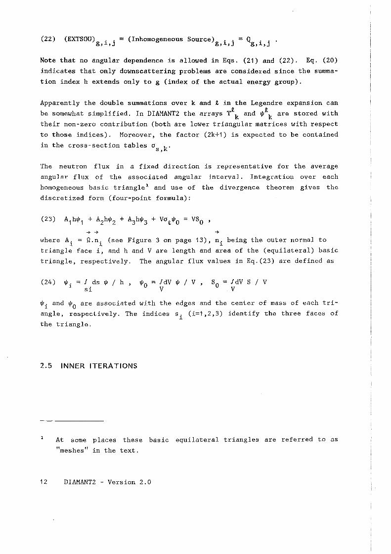
Figure 3. Coefficients of the Differential Equation

Figure 4. Passihle Grientations of a Triangular Gell

Figure 5. Sequence of Directions in an S4 Calculation

Figure 6. Space-Angle-Mesh-Sweep Grdering

Figure 7. Computational Mesh Sequence for Fixed Direction

Figure 8. Passihle Grientations of the System Boundary

4

9

13

14

16

17

18

26

Figure 9. Cross Reference Table for Subroutine Calls 31

Figure 10. Array Allocation in A(NACMAX) resp. DBN=DIAM21SREAL•'(4 46

Figure 11. Usage of Arrays BIL1,BIL2,BIL3 48

Figure 12. Array Allocation in IW (NWMAX) resp. DBN=DIAM21SINTEGER•'(4 49

Figure 13. Use of CGMMGN Blocks by Subrautirres 50

Figure 14. Usage of CGMMGN /CGMARR/ 53

Figure 15. Usage of CGMMGN /COMBND/ and CGMMGN/CGMCHA/ 54

Figure 16. Usage of CGMMGN /CGMLGG/ 54

Figure 17. Usage of CGMMON /CGMINT/ 55

Figure 18. Usage of CGMMON /CGMPGI/ 60

Figure 19. Usage of CGMMON /CGMREA/ 61

Figure 20. Usage of CGMMGN /CGMSTG/ and BLANK COMMGN 62

Figure 21. Usage of CGMMGN /FILLCG/ and CGMMGN /FILLCX/ 62

Figure 22. Data Files und Their Use 64

Figure 23. Structure of the Label Record in Restart Dump Files 67

Figure 24. Recommended Content of DBN = INITISREADISDIAMAN, IND = 71

Figure 25. Dependence of DIAMANT2 on KAPRGS 73

Figure 26. Examples for Storage, CPU Times and Execution Speed 81

Figure 27. CPU Times for Same Vector Computers (Isotropie Scattering) 84

Figure 28. CPU Times for Same Vector Computers (Anisotropie Scattering) 85

Figure 29. Definition of PARAMETER Values Used in DIAMANT2 87

Figure 30. PARAMETER Values Used on Different Computers 88

Figure 31. Basic Input Zones ITYP 101

Figure 32. Convexity of the Model Boundary 107

Figure 33. Specifying the Model in the Reference Parallelegram 108

Figure 34. Storage Sequence in Cross Section Array C 109

Figure 35. Example of an External Source Input 111

Figure 36. Example of a Boundary Flux Input 113

List of Illustrations ix

x DIAMANT2 - Version 2.0

CHAPTER 1. INTRODUCTION

DIAMANT2 (release 2. 0) is an improved version of the DIAMANT 111, 121 program

for two-dimensional neutron transport calculations in planar geometry using

a regular triangular mesh. The program solves both regular and adjoint,

homogeneaus or inhomogeneous, time-independent problems subject to vacuum,

reflective or input specified boundary flux conditions.

DIAMANT2 is a fully FORTRAN77 conforrning code designed to run on many dif

ferent computers as efficiently as possible. It successfully solved a set

of standard test problems on IBM, FACOM, CYBER-205, CRAY and SIEHENS VP

series computers. Many functional improvements have been incorporated:

1. Anisotropie scattering option now operational;

2. New option to create interface files for use in the perturbation module

TPTRIAI31;

3. Use of an effective absorption implied by the input cross sections;

4. New built-in quadrature sets and higher SN orders;

5. Improved inner-outer iteration strategy;

6. Several convergence criteria as user option;

7. Clean-up of the coding (FORTRAN77) and restructuring;

8. Elimination of installation dependent routines;

9. Centralization of binary inputloutput operations;

10. Re-organization of computer memory usage;

11. Complete input control print is provided prior to execution;

12. Special care has been taken to allow efficient execution on vector com

puters.

Details of these features as well as a complete description of all options

of DIAMANT2 are given in the following chapters. In the next chapter, dif

ference equations and solution algorithms are discussed. Chapter 3 is a guide

for implementation and chapter 4 contains information relevant to the user

of DIAMANT2. Chapter 5 is the KAPROSI41 short description of the module.

The input description is contained in Chapter 6. The last chapter gives a

complete example of a DIAMANT2 run along with an output description.

Part of this document (especially Chapter 2) has been influenced by the

TWOTRANI51 manual.

Chapter 1 . Introduction

2 DIAMANT2 - Version 2.0

CHAPTER 2. DIFFERENCE EQUATIONS AND SOLUTION ALGORITHM

2.1 ANALYTIC FORM OF THE STATIC NEUTRON TRANSPORT EQUATION

The time independent neutron transport equation is written as

(1)

Q.V~(r,E,Q) + ot~(r,E,Q) = -+ -+ -+ -+ -+ -+

ldE'!dQ'$(r,E' ,Q')o (r,E'-+E ,Q'-+Q) s

-+ -+ -+ -+ -+ -+

+ X(E) fdE'!dQ'$(r,E' ,Q')vof(r,E 1 )/(4TI) + Q(r,E,Q)

in which $ is the particle flux (number density of particles times their

speed) defined such that $dVdEdQ is the flux of particles in the volume

element dV about ~ in the element of solid angle dQ about ?.!, in the energy """ range dE about E. Similarly, QdVdEdQ is the nurober of particles in the same

element of phase space emitted by sources independent of $. The macroscopic

total interaction cross section is denoted by ot' the macroscopic scattering

I ~ -transfer probability (from energy E to E and from angle Q to angle Q) by

Os' and the macroscopic fission cross section by of. (all these quantities

depend on 1, but we have omitted this argument for simplicity). The nurober

of particles emitted isotropically (1/4TI) per fission is v, and the fraction

of those liberated in the range dE about Eis X(E). This fraction may actu

ally depend on both, the material undergoing fission and the energy of the

fission inducing neutron, but such possibilities are not admitted in

DIAMANT2. The influence of that effect may be estimated by using the per

turbation theory module TPTRIA /3/.

2. 1.1 Divergence Operator

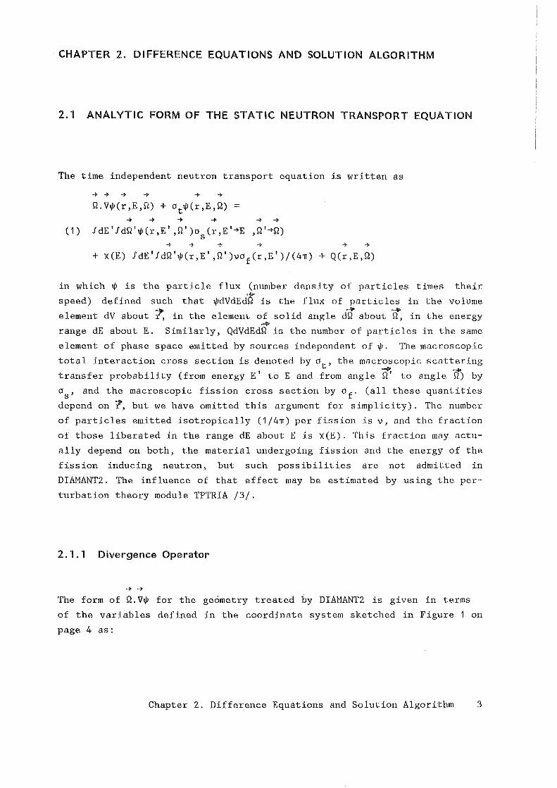
-+ -+ The form of Q.V$ for the ge6metry treated by DIAMANT2 is given in terms

of the variables defined in the coordinate system sketched in Figure 1 on

page 4 as:

Chapter 2. Difference Equations and Solution Algorithm 3

I I I I I I I I I I I I I I I I I I I

----+ ~ ',, 0 ',

--------- ___ :~ ~

/

'\ l ' I ',I .. •' I

'j!.'·~------------- I

X

-r

-I Figure 1. Coordinate System Used in DIAMANT2

Dependence of lJl !JJ(x,y,}.l,11,E) -+ -+ -+ -+

Definition of Variables ll = e .n ' 11 = e .n X y

-+ -+

Streaming operator n.V!JJ = (lla;ax + 11a;ay)

z

y

lJl

-+

~ is the angle of rotation about the ll axis such that dQ can be replaced

by d}.ld~, and

~ = /(1 }.l 2) sin ~

(2) 11 == /,....(-1 --ll-:-2 .,)9 cos ~

ll = /(1 112 - ~ 2 ) •

I I I I I I I I I I I I I I I I I I I I

JjJ is assumed to be symmetric in ~, and only a hemisphere of angular

directions needs to be considered. The north pole of the hemisphere points

in z-direction.


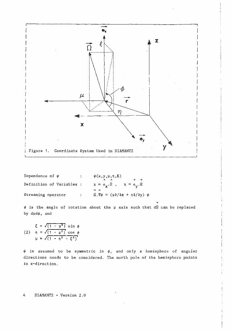
2.1.2 Spherical Harmonics Expansion of the Scattering Source Terms

The scattering kernel o is assumed to be representable by a finite Legandre s - -polynomial expansion (implicitly assuming that the scattering Q'~Q is ~ ~

dependent on the cosine Q' .Q only)

If this expansion is inserted in Eq. (1), and if the addition theorem is used

to expand Pk(~0 ), we can write

(3) -t -t -t

ldE'JdQ'~(r,E' ,Q') o (E'~E,~o) = s

'i'(

where o sk = (2k+1)/(4TI)Osk'

In deriving this expression, the ~ symmetry of ~ is used, reducing the domain ...;.

of Q to a hemisphere and eliminating expansion terms odd in~. The functions

T~ are defined by

(4)

where ö~k is the Kronecker delta (equal to 1 if ~ = k, and vanishing other

wise) and the P~ are the associated Legandre polynomials.

Hence, if the angular flux is expanded into a series of these functions,

ISCT k (6) ~ =}: (2k+1) }: T~ V'~'

k=O ~==0

the expansion coefficients are given by

(7)


Using this formula, we can rewrite Eq. (1) as

(8)

+ X(E) /dE' vof(E')~~ + Q

As implied by this equation, we have assumed that the source Q is isotropic,

e.g., not dependent on the angular variable.

2.2 MULTIGROUP EQUATIONS

The energy domain of interest is assumed to be partitioned into IGM intervals

of width AEg' g = 1, 2, ... , IGM. By convention, increasing g represents

decreasing energy. If we multiply Eq. (8) by AE and integrate we can write g

-+ -+ (9) Q.'ill/J + ot 1/J g ,g g

IGM ISCT k ~ ~ = L E (2k+1)o k h-+ L Tkl/Jk h

h=1 k=O s, ' g ~=0 '

IGM 0 + Xg L vofhl/JO,h + Qg , g=1, ... ,IGM

h=1

Here, the flux, 1/J , as well as the fission spectrum, X , for group g g g

(10) 1/Jg = /dE 1/J , Xg = /dE X(E)

AE AE g g

are no langer distributions in energy, but refer to the total number of

partielas in the energy interval. For this reason, if group structures are

changed, the effect on results must be evaluated by comparing 1/J /AE . Because g g of Eq. (10), energy integrals in DIAMANT2 are evaluated by simple sums.

Cross sections subscripted with g are weighted averages in energy group g,

e .g.,


(Ha) otg = ( fdE Otl/1) 1 ( fdE $)

~E ~E g g

The transfer cross sections 0 k h~ are flux moments weighted averages in s, , g group h and integrals over the inscatter group g :

( 11 b) 0 = ( /dE /dE' 0 (E'~E) Ll/I~(E')T~ ) I JdE' Ll/I~(E')T~ s,k,h~g s,k ~ k k ~ k k

Of course, ~ is not known in advance and must be approximated by some means.

This has tobe clone in aseparate code. If in Eq. (11) the angular dependence

of l/1 is nonseparable, then otg will in principle be angle-dependent. No

provision for such dependence is made in DIAHANT2.

Within the code only downscattering problems can be solved which means that

the first summation in Eq. (9) does not extend to h=IGM but to h=g only.

Equation (9) is solved using a conventional inner-outer iteration procedure

as described in the following text.

2.3 DISCRETE ORDINATES APPROACH

To approximate the angular dependence, we select JMM directions on the unit

sphere and require Eq.(9) to hold only for these directions. Omitting the

group index, we end up with a coupled system of equations

(12) Qm.Vl/lm + o l/1 = S lJI = lJI(r,Q ) t m m' m m S = S(r,Q ) m m

The scalar, i. e. angle- integrated, flux is approximated by a quadrature

formula

(13) </l (r) JMM

= r m=1

l/1 (r) m

where the wm are the integration weights associated with direction Qm' and

JMM is the total number of directions used.


2.3. 1 SN-Constants and Angular Orientation

For a quadrature order ISN, DIAMANT2 requires JMM = ISN~'~'(ISN+2)~'~'3/4+ISN pairs

(J..I,ll) of direction cosines. These are, for ISN up to 12, provided by the

subroutine SNCONS (the upper limit 12 is fixed by a PARAMETER statement).

The code actually uses only JM:t-1-ISN directions, the remaining directions,

having an integration weight zero, arenot used by DIAHANT2 and are included

only for historical reasons.

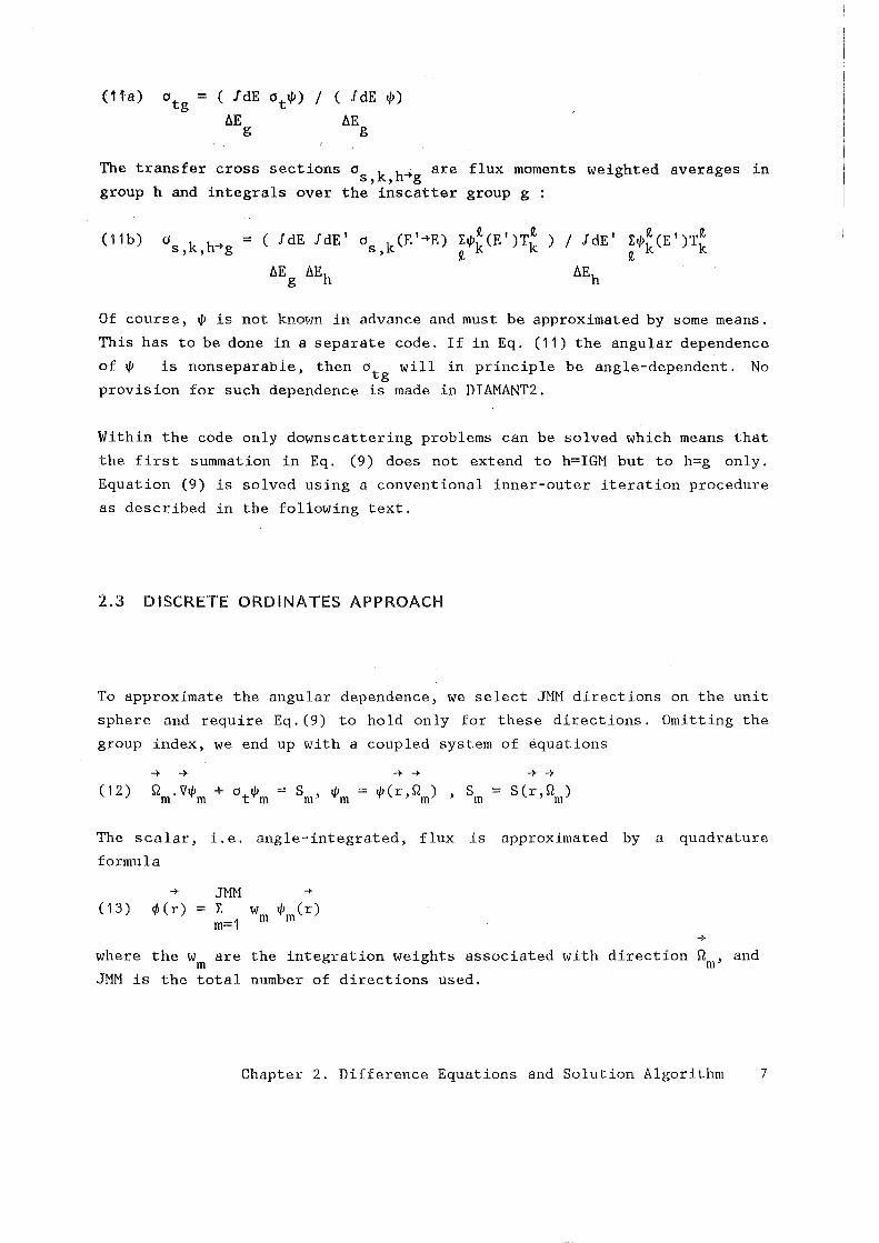
2.3.2 Construction of SN-Constants

SN-constants are built-in in the code. Presently, a user may choose by input

among three different sets : PN, DPN and EPN. Same hints, as to which one

of them should be used in a particular application, are given in "How to

Choose the Quadrature Set" on page 78. The constants used are described in

"Appendix A. DIAMANT2 Built-in Quadrature Constants" on page 119. The con

struction itself consists of the following steps:

1. We subdivide the upper unit hemisphere into six sixty degree sectors

(called "dodecants").

2. For each dodecant we select n=ISN/2 level lines (where ISN is the quad

rature order selected and is supposed tobe an even number).

3. Each level line is assigned a value of ~; the ~-value is taken from a

1d quadrature set (presently possible: PN, DPN and EPN set) as well as

the associated integration weight.

4. To calculate J..l and n according to Eq. (2), we still have to define the

angle I. In DIAMANT2 we request:

(14) lj = (2j-1) TI I 6k, j=1, ... ,k k=1, ... , ISN/2

(see Figure 2 on page 9).

5. The integration weight associated with a certain level is distributed

uniformly among all angular points on that level.


I I I I I I I I I I I I I I I I I I I I I I I I I I I Figure 2.

'fli12

~ QUADRATURE POINTS S,. QUADRATURE POINTS

.. · \

.... ··········'·········· 7T/18 'i

56 QUADRATURE POINTS S8 QUADRATURE POINTS

Construction of Quadrature Constants

-t

Several desirable relationships between the projections ~ and n of ~ on m m m the coordinate planes, and the integration weights w are fulfilled for the m built-in quadrature sets (all sums extend from m=1, ... ,JMM):

(i) Normalization: }: w = m

(15) ( ii) Equilibrium: E wm~m = E w n = 0 m m

(iii) Diffusion consistency: E w ~2 = E w n2 = 1/3 m m m m


2.3.3 Boundary Conditions

-+ -+

Information about incoming boundary fluxes (Q.n < 0) can be specified by

the DIAMANT2 user Details on the input specification are given in "Boun

dary Fluxes" on page 112. One may select any meaningful combination of the

three following options for the geometrical solution domain but on each

boundary mesh line only one type of boundary condition can be applied.

2.3.3. 1 Vacuum Boundary Condition

The value of the angular flux ~ on such a boundary is set to zero for all

incoming directions.

2.3.3.2 Reflective Boundary Conditions

The value of the flux on such a boundary for incoming directions is set equal

to the value of the outgoing flux in the reflective direction.

2.3 .3 .3 Boundary Fluxes

On any side of the solution domain, the user may specify isotropic boundary

fluxes. These inflows represent a source of particles and are treated as

such by the code. Use of this option implies an inhomogeneaus calculation.


2.4 DIFFERENCE EQUATIONS

To discuss the spatial finite difference representation, we write Eq. (9)

for a single energy group and a single direction as

(16) Q.V~ + ot~ = S ,

omitting the group and the direction subscript. On the right-hand side of

eq. (9) the integral

( 17) 11-

~k,h =

is approximated for each group h by the sum

(18) 11-TFk h ..

' '1' J

JMM II-= L w Tk(~ ,~ )FLXANGh .. m= 1 m m m , 1 , J , m

where JHM is the total number of directions, cf> is defined by the program m

as

-1 c/c1 2 2 I ( 19a) cf>m = tan - llm - nm) I nm) if nm > 0

'

-1 c/c1 2 2 I (19b) cf>m = tan ll - nm) I n ) + 1T if nm < 0

m m

and II-TFk h ..

' '1, J is the

ll, value of ~k,h in spatial cell (i,j).

0 In the code TF0 h is identified with the scalar flux FLXSKAh. ' The right-hand side of Eq.(16), S = S .. , is given by the sum of the g,1,J,m

following three contributions:

(20) (SS) . . = (Scatter Source) . . = g,1,J,m g,1,J,m

g ISCT k ll, 11-

r r (2k+1)o k h~ }; Tk TFk h . · , h=1 k=O s, ' g ll,=O ,m ' > 1 >J

(21) IGM

(FG) . . = (Fission Source) . j = X }; vof,h TF00 h . . g,1,J g,1, g h=1 ' ,1,J


(22) (EXTSOU) . . = (Inhomogeneous Source) . . = Q . • • g,1,J g,1,J g,1,J

Note that no angular dependence is allowed in Eqs. (21) and (22). Eq. (20)

indicates that only downscattering problems are considered since the summa

tion index h extends only to g (index of the actual energy group).

Apparently the double summations over k and ~ in the Legendre expansion can

be somewhat simplified. In DIAMANT2 the arrays T~k and ~~k are stored with

their non-zero contribution (both are lower triangular matrices with respect

to those indices). Moreover, the factor (2k+1) is expected tobe contained

in the cross-section tables o k' s'

The neutron flux in a fixed direction is representative for the average

angular flux of the associated angular interval. Integration over each

homogeneaus basic triangle 1 and use of the divergence theorem gives the

discretized form (four-point formula):

-t -t

where Ai = Q.ni (see Figure

triangle face i, and h and V

triangle, respectively. The

-t

3 on page 13), n. being the outer normal to 1

are length and area of the (equilateral) basic

angular flux values in Eq.(23) are defined as

(24) = J ds ~ I h , si

~0 = fdV ~ I V V

so = J dV s I V V

~i and ~O are associated with the edges and the center of rnass of each tri

angle, respectively. The indices s. (i=1 ,2,3) identify the three faces of 1

the triangle.

2.5 INNER ITERATIONS

At some places these basic equilateral triangles are referred to as

"meshes" in the text.


c

c*cos(1T/6-t) c~\-cos ( t+1T /6)

~ defined by Eq. (2), t defined by Eq. (14).

Figure 3. Coefficients of the Differential Equation

2. 5.1 Diamond Difference Approximation

-t

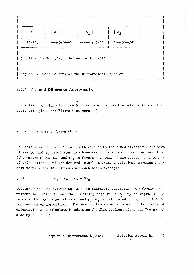
For a fixed angular direction Q, there are two possible orientations of the

basic triangles (see Figure 4 on page 14).

2.5.2 Triangles of Orientation 1

For triangles of orientation 1 with respect to the fixed direction, the edge

fluxes ~ 1 and ~2 are known from boundary conditions or from previous steps

(the vertex fluxes ~B 1 and ~B 2 in Figure 4 on page 14 are needed by triangles

of orientation 2 and are defined later). A diamond relation, assuming line

arly varying angular fluxes over each basic triangle,

(25) ~1 + ~2 + ~3 = 3~o

together with the balance Eq.(23), is therefore sufficient to calculate the

unknown box value ~O and the remaining edge value ~3 ; ~O is expressed in

terms of the two known values ~ 1 and ~2 . ~3 is calculated using Eq.(25) which

implies an extrapolation. For use in the solution step for triangles of

orientation 2 we calculate in addition the flux gradient along the "outgoing"

side by Eq. (26d).


I I I I I I I I I I I I I I I I I

o rinown • lmown

ORIENTATION 1

0 unlmown • known

1/JB1

ORIENTATJON 2

I The arrow at the top of the figure indicates the assumed direction

I I I

of neutron travelling.

I Figure 4. Passihle Grientations of a Triangular Gell

(26a) t/J = (Vv~·~s + (A -A )~·~.p + (A3 -A2 )~·~.p 2 )/NENN 0 0 3 1 1

(26b) NENN = 3~'~A + STOT~·~vv 3 VV = V/h

This approximation is locally O(h 2) accurate since only the linearity

assumption, Eq. (25) is needed. ("locally O(h 2)" means that for small mesh

steps h, the magnitude of the (local) truncation error over each basic tri

angleisproportional to a term of order h 2 ). Use of a fix-up may be required

for certain mesh cells since the extrapolation using Eq.(25) may possibly

yield physically unreasonable negative flux values.


2.5.3 Triangles of Orientation 2

For triangles of orientation 2, only ~3 of the three edge values is known.

To calculate the remaining two, ~ 1 , ~2 , as well as ~0 , one further relation

independent of Eqs.(23) and (25) is needed.

Walters et al. /6/ describe an effective scheme using the flux values at the

corners and the centers of the triangle sides (seven-point formulation).

Using the basic idea of this scheme for DIAHANT2 requires that the four-point

formulas, Eqs. (23) and (25), are extended; instead of using only the cen

tered values on the triangle sides, flux gradients along the triangle sides

are calculated as well. For orientation 1 triangles, the auxiliary value

~B 1 -~B 2 (see Figure 4 on page 14), is calculated and temporarily stored

(thereby using the assumption of linearly varying flux over each triangle

cell). Then, for orientation 2 triangles, ~3 is known as well as the flux

gradient along triangle face s 3 - and therefore it is possible to calculate

~ 1 , ~2 , and ~O using Eqs. (23), (25) and (26) and the linearity of fluxes

over the triangle. Use of a fix-up may be required since the extrapolations,

Eqs.(25) and (26), may possibly yield physically unreasonable negative flux

values.

VV = V/h

(28a) ~ 1 = ~3 + ~B1

(2Sb) $2 = ~1 - ~B1 + ~B2

2.5.4 Negative Flux Fix-Up

As mentioned before, Eqs. (26) to (28) may sometimes result in negative

angular fluxes. As these are physically unreasonable, they are eliminated

by switching to a (positive) step scheme. In any case $ 0 is always positive


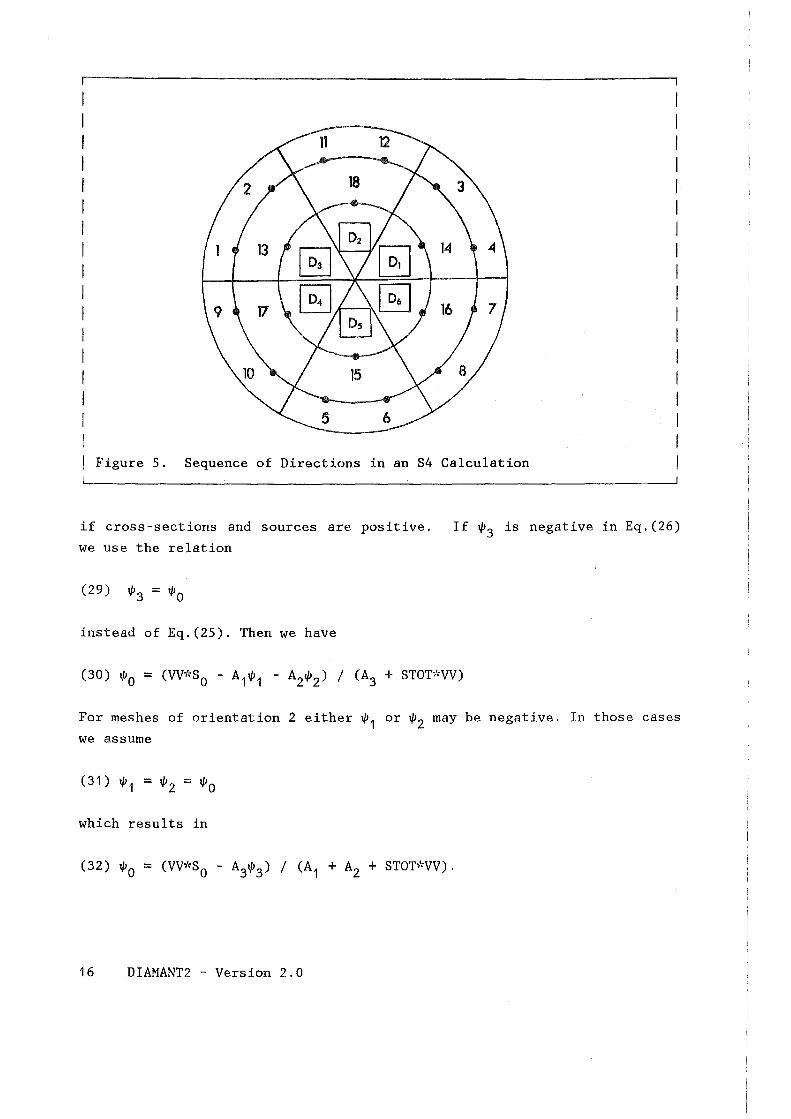
Figure 5. Sequence of Directions in an S4 Calculation

~------------------------------------------------------------~

if cross-sections and sources are positive. If tP3 is negative in Eq. (26)

we use the relation

instead of Eq.(25). Then we have

For meshes of orientation 2 either tP 1 or tP2 may be negative. In those cases

we assume

which results in


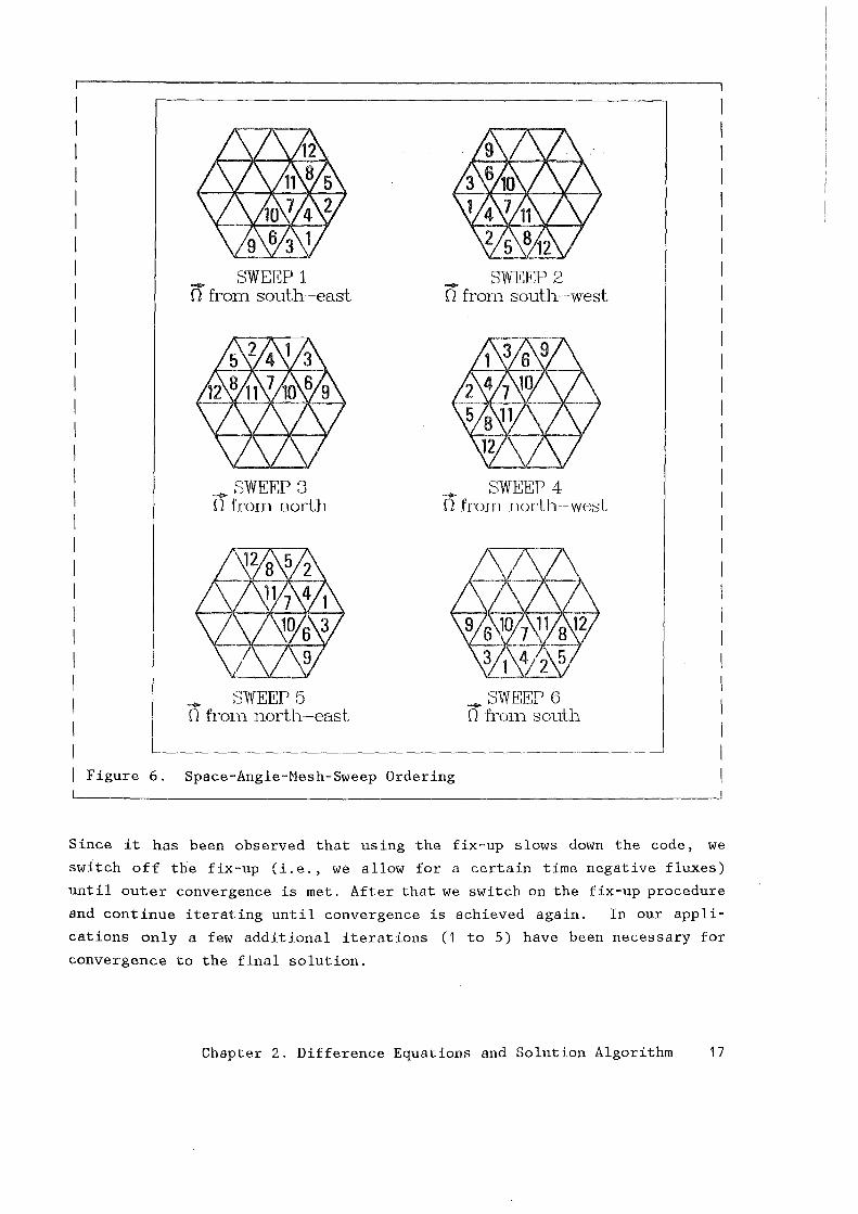
I I I I I I I I I I I I I I I I I I I I I I I I I I I I I I Figure 6.

- SWEEP 1 - SWEEP 2 0 from south-east 0 fron1. south-west

_ SWEEP 3 - SWEEP 4 0 from north n frorn north~-west

- SWEEP 5 -SWEEP 6 0 fron1. north-east 0 fron1. south

Space-Angle-Nesh-Sweep Ordering

Since it has been observed that using the fix-up slows down the code, we

switch off the fix-up (i. e., \ve allow for a certain time negative fluxes)

until outer convergence is met. After that we switch on the fix-up procedure

and continue iterating until convergence is achieved again. In our appli

cations only a few additional iterations (1 to 5) have been necessary for

convergence to the final solution.


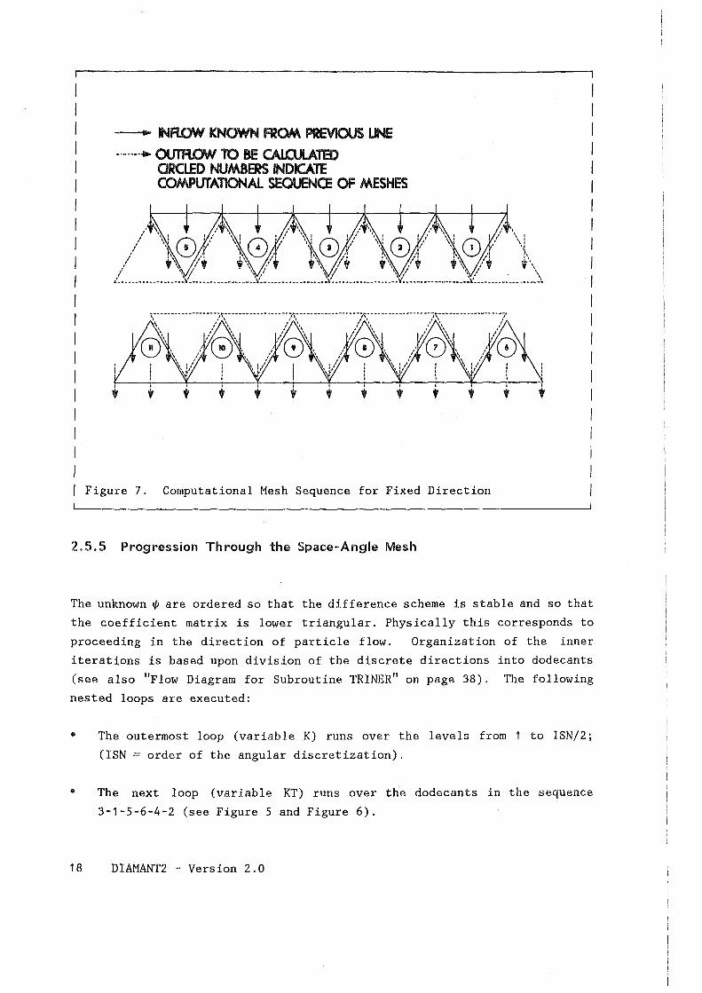
--.... INR.OW KNOWN FROh\ PREVJOUS UNE

-------• OUTROW' 10 BE CAI.CULATED ORCLED NUMBERS INDICATE COMPUTATIONAL SEOUENCE OF MESHES

Figure 7. Computational Mesh Sequence for Fixed Direction

2.5.5 Progression Through the Space-Angle Mesh

The unknown ~ are erdered so that the difference scheme is stable and so that

the coefficient matrix is lower triangular. Physically this corresponds to

proceeding in the direction of particle flow. Organization of the inner

iterations is based upon division of the discrete directions into dodecants

(see also "Flow Diagram for Subroutine TRINER" on page 38). The following

nested loops are executed:

•

•

18

The outermost loop (variable K) runs over the levels from 1 to ISN/2;

(ISN = order of the angular discretization).

The next loop (variable KT) runs over the dodecants in the sequence

3-1-5-6-4-2 (see Figure 5 and Figure 6).

DIAMANT2 - Version 2.0

•

•

•

The next loop (variable K2) sweeps over all directions on level K in

dodecant KT.

The next to last loop (variable I) runs through the "line" of the dis

cretization grid (the definition of a "line" is dependent upon the

dodecant in which the directions are being considered , see Figure 6 on

page 17 and Figure 7 on page 18).

The last loop (variable J) finally processes the individual triangles

of each line (see Figure 7 on page 18 ).

We thus arrive at the sequence of space-angle sweeps shown in Figure 6 on

page 17. The control information required for selection of the next direc

tion and the next triangle is kept to a minimum. Moreover, the innermost

loop solves Eq. (23) for all meshes on a line simultaneously. This is

important with respect to the vectorization potential of the DIAMANT2 code

(see "Experiences on Vector Computers" on page 83).

2.5.6 Inner Convergence Tests and Convergence Aceeieration

Depending on input specification, there are two criteria to test convergence

of inner iterations. Both of them test groupwise the deviation of scalar

fluxes during two successive inner iterations.

(33) f:. 1-nner = LI ~old _ ~new I I L ~new

0 0 0

is called "integral" test and is used whenever the input variable EPSA is

less then zero. The Summation extends over all mesh cells. Note that for

regular triangular geometry (constant mesh volume) the summation is equiv

alent to a spatial integration.

(34) f:. =maxi 1.0 1-nner ~old I ~new

0 0

is called "point-wise" test and is used whenever EPSA is greater or equal

to zero. The maximum is taken over all mesh cells. Note that this criterion

puts emphasis on the local behaviour of scalar fluxes.

morestringent than (33).

Test (34) is much


Inner iterations are stopped if t. ~ I EPSINN I. The value of EPSINN 1nner depends on the accuracy ERROUT reached in the previous outer iteration. In

order to avoid too many inner iterations during the initial phase of outer

iterations we set:

EPS INN = max ( min ( 0. 1 ~'~'ERROUT, EPS INN) , I EPSA I )

after each outer iteration. For the first outer iteration, EPSINN is ini

tialized to 1 .OE-1 (1.0E-3 if a restart durop is being used).

This special prescription of inner iteration accuracy has been chosen in

order to give a roore srooothly eigenvalue convergence. It is guaranteed that

the flux error is non-increasing. At the cost of roore outer iterations, the

total nurober of iterations is usually decreased (for equivalent accuracy)

as coropared to the older version of DIAMANT2.

Irrespective of the value of E. , inner iterations are stopped if the 1nner nurober of iterations is bigger than the value of variable IU1AX. This is

initialized with the input value of IIL and increased froro one outer iter

ation to the next by one until the input value of IIM is reached.

Only one inner iteration acceleration roethod has been iropleroented in DIAMANT2

up to now, naroely global rebalancing for the inner iterations. The group

dependent rebalancing factors

(35) FUN = L S . / L(S . + o ~ .*(~ n~w - ~ o~d)) g g,1 g,1 g-rg,l. g,1 g,1

are calculated in each inner iteration. S . is the suro of the neutron g,1 sources in energy group g in roesh cell i. The suroroation extends over all

roesh cells. No rebalancing is atteropted in boundary flux cases. If FUNg

is 1.0 within a certain threshold or becoroes negative, rebalancing is skipped

too. All scalar fluxes and the leaking angular fluxes are then roultiplied

by the factor FUNg. Global neutron balance is roaintained in this roanner (see

/8/).


2.6 OUTER ITERATION PROCEDURE

The discretized multigroup neutron transport equations form a linear

equation system:

(36a)

(36b)

(36c)

L~'(u = sf + ss~~u + Q ext

Sf = F~~u/k eff

S = F~~u f

for homogeneaus problems

for inhomogeneaus problems

L describes the lasses, Sf the fission source, 88

the scattering matrix, F

the fission matrix and Q t the (possibly existent) external source. u is ex the vector of the flux values at the triangle centers, keff is the desired

(dominant) eigenvalue of the problern (criticality factor). S is lower tri-s

angular since no up-scattering is allowed. Equations (36) are solved by

means of the conventional power method (''fission source" or "outer" iter

ation): (j=O, 1, 2 ..... )

(37a) U'u (j+1) = sf (j) + S ~~u (j+1)

s

(37b) sf (j+1) = F~'<'u (j+1) jk (j)

(37c) k (j+1) = k (j ) ~'<'}: ( F~''u (j + 1 ) ) I l: (F~'•u (j)) (homogeneous problems)

(37d) k (j+1) = (inhomogeneous problems)

In (37c), the summation extends over all mesh points and all energy groups.

k~i~ converges to the criticality factor, keff' as the number of iter-

ations increases; Sf(o) is dependent upon the source guess used (source equal

to 1.0 for all meshes as adefault option).

An additional speed-up of the whole calculation can be achieved by the use

of a source and flux guess taken from a previous calculation. Only guesses

using an identical space-angle-energy mesh grid will be accepted. This

option is very useful in calculations with anisotropic scattering. It is

highly desirable first to establish a reasonably converged flux guess using


isotropic scattering and then starting the anisotropic scattering calcu

lation using that guess.

Depending on input specification, there are three criteria to test conver

gence of outer iterations. All of them test the deviation of the sum of all

neutron sources s 0 between two successive outer iterations (sums extending

over all meshpoints):

(38) E = EI Sold - Snew I I E Snew outer 0 0 0

is called "integral" test and is used whenever the input variable EPS is less

then zero.

(39) E t = maxi 1 .o - soold I snoew I ou er

is called "point-wise" test and is used whenever EPS is greater than zero.

This criterion puts emphasis on the local behavior of the source distrib

ution.

The third possibility is a test based on eigenvalue bounds which is used

whenever EPS is equal to zero:

(40a) E = k - k 1 where out er u

(40b) k u = max Sold 0 I snew

0

(40c) kl = min Sold I snew 0 0

ku and k 1 are upper and lower eigenvalue bounds.

Outer iterations are stopped if E t $1 EPS I. In case EPS = 0.0 the code ou er

uses the value of TEPS. Tests (39) and (40) are much more stringent than

(38). Test (40) avoids premature iteration termination in slowly convergent

cases where the source distribution changes are small from one iteration to

the next, but leads to increased CPU time consumption.

Outer iterations are stopped too if either the maximum number of outer

iterations is. reached (input variable ICM) or if CPU time is near to

exhaustion. The code measures the CPU time t t needed for each outer Oll

iteration. Using the timing function TIMLIN it gets then the amount of CPU


time still left and breaks the iteration whenever 3'>'rt t is smaller than the ou remaining CPU time. Depending on the accounting system, t t may not have

ou the dimension of a time (e.g. on CYBER-205 it is measured in System Billing

Units). Function TIMLIM usually has to be rewritten for a new computer

(available for IBM and compatibles, CYBER-205 and GRAY).

2. 7 OTHER CODE OPTIONS

2. 7.1 Adjoint Calculations

DIAMANT2 solves the adjoint transport equation in the usual way /8/:

1. The scattering matrices are transposed.

2. The role of vof and X are exchanged.

3. The energy group order is reversed.

4. The solution for angle Q is identified with angle -Q (of the adjoint m m problem).

Formally, (1.) transforms the orginal down scattering problern into an up

scattering problem, but (3.) converts it to a formal down scattering problern

again. It should be noted that the group numbers will be inverted in input

and output, i.e., energy group 1 in adjoint computations corresponds to the

lowest energy range. Moreover, the order of energy groups and of directions

(according to (4.)) aretobe inverted for the input of bucklings, boundary

fluxes and flux guesses. Only input of nuclear cross sections is the same

in real and adjoint problems. The user should be aware that fluxes and

source terms are group integrals in direct calculation, whereas adjoint

fluxes and source terms must be understood as group averaged values, in

accordance with (1.) and (2.) (see also the comments concerning group

averaged and group integrated quantities in "Multigroup Equations" on page

6).


2. 7.2 lnhomogeneous Calculations

Inhomogeneaus calculations can be specified using either boundary fluxes or

external sources.

External sources arenot allowed to be anisotropic. They may be input in four

options

1. for all groups and all meshes;

2. for all meshes along with a global energy spectrum;

3. for all groups and all mixtures;

4. for all mixtures along with a global energy spectrum.

Boundary fluxes are not allowed to be anisotropic. They may be input in two

options

1. for all groups and all sides containing sources;

2. for all sides containing sources along with a global energy spectrum.

In those· cases where a global energy spectrum is used, the group dependent

source distribution is determined as the product of the source strength

specified for the mesh, mixture or side, respectively, times the input energy

spectrum. No normalization to unity of the energy spectrum is clone by

DIAHANT2.

2. 7.3 Evaluations and Balances

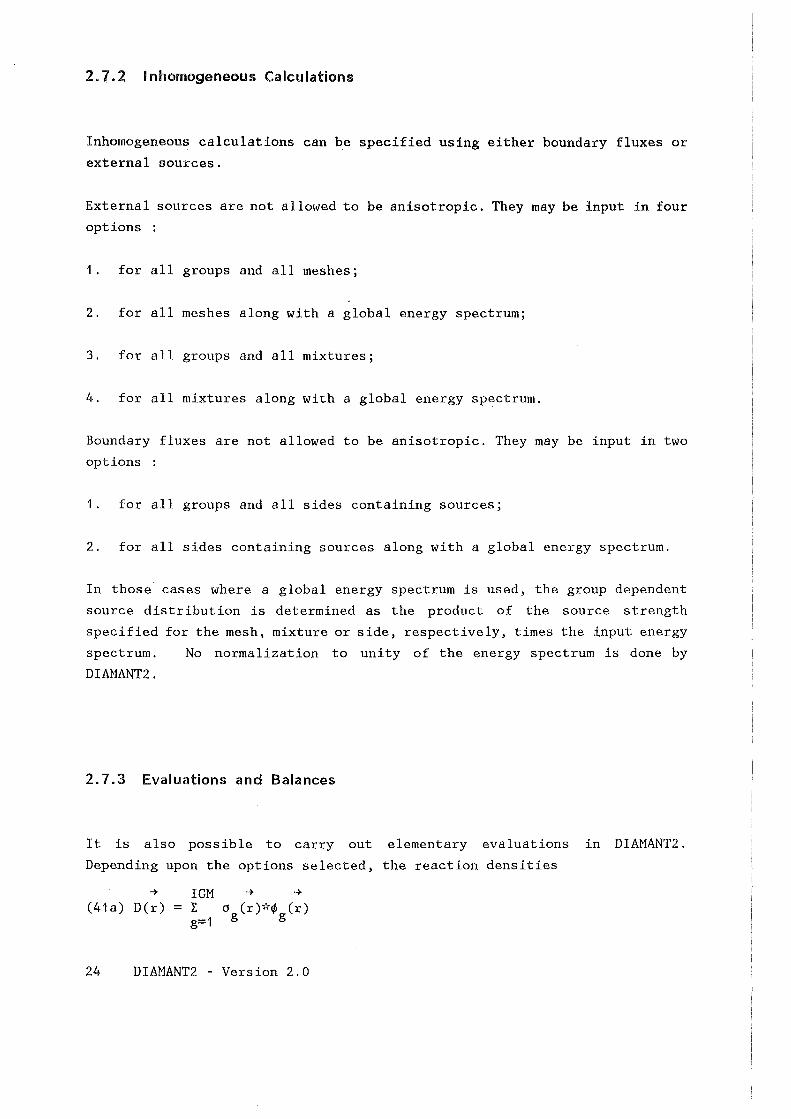
It is also possible to carry out elementary evaluations in DIAMANT2.

Depending upon the options selected, the reaction densities

-+ IGM -+ -+ (41a) D(r) = E a (r)*- (r)

g=1 g g


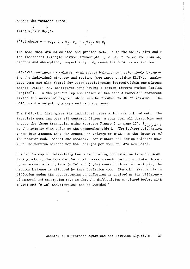
and/or the reaction rates:

~ ~

(41b) R(r) = D(r)*V

for each mesh are calculated and printed out. ~ is the scalar flux and V

the (constant) triangle volume. Subscripts f, c, a, t refer to fission,

capture and absorption; respectively. ot means the total cross section.

DIAMANT2 routinely calculates total system balances and selectively balances

for the individual mixtures and regions (see inputvariable KAUSW). Analo

gaus sums are also formed for every spatial point located within one mixture

and/or within any contiguous zone having a common mixture nurober (called

"region"). In the present implementation of the code a PARMIETER statement

limits the nurober of regions which can be treated to 30 at maximum. The

balances are output by groups and as group sums.

The following list gives the individual terms which are printed out. The

(spatial) sums run over all centered fluxes, m runs over all directions and

k over the three triangular sides (compare Figure 8 on page 27). ~ t k . m,g,ou , is the angular flux value on the triangular side k. The leakage calculation

takes into account that the amounts on triangular sides in the interior of

the reactor model cancel one another. For mixture and region balances nei

ther the neutron balance nor the leakages per dodecant are evaluated.

Due to the way of determining the outscattering contribution from the scat

tering matrix, the term for the total lasses exceeds the correct total lasses

by an amount arising from (n,2n) and (n,3n) contributions. Accordingly, the

neutron balance is affected by this deviation too. (Remark: frequently in

diffusion codes the outscattering contribution is derived as the difference

of removal and absorption rate so that the difficulties mentioned before with

(n,2n) and (n,3n) contributions can be avoided.)


N

sw SE

s Figure 8. Passihle Grientations of the System Boundary

Individual Terms in Balancing Output (Group Dependent)

External source

Fission source

I nscatter source in group g

Total production

Total flux

Fission production

Within-Group scattering

Absorption


G I xg~'( l: l: vof,h(i)~'(q,h(i)

h=1 i=1

g-1 I l: l: oh-+g(i)~'(!flh(i) h=1 i=1

External source + Fission production + Inscatter source

I l: 1/! (i) i=1 g

Fission source/keff

I l: o...-+g(i)~~I/Jg(i) i=1 5

I l: i=1

0 (i)~~q, (i) a,g g

Buckling leakage

Out-scattering from group g

Total leakage

Total Iosses

Capture density

Fission density

Neutron balance

Leakages from the 6 dodecants

I ! i=1

B2(i)*f (i)/(3*a (i)) g g tr,g

Sum of the 6 individual leakages (see

below)

Absorption + Leakage + Out-scattering

I t i=1

I t i=1

a (i)~"f (i) c,g g

C1 (i)~'•rt> (i) f,g g

Total production / Total lasses

M 3 t L. m=1 k=1

w *A *~ *h m k,m m,g,out,k

Here, I is the total number of spatial meshes, G the number of energy groups

and M the number of discrete directions. In the last formula, w and Ak m ,m are the constants defined in 11 Construction of SN-Constants 11 on page 8 and

"Diamond Difference Approximation" on page 13, respectively. h is the con

stant length of a triangle side.


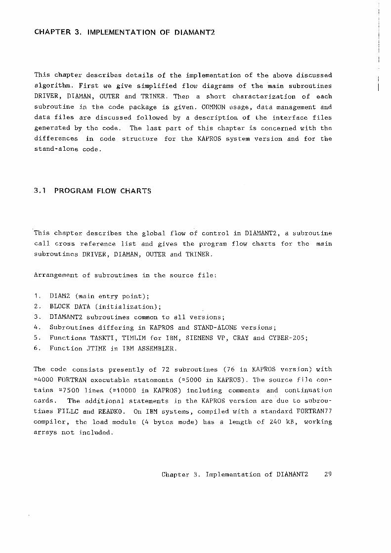
CHAPTER 3. IMPLEMENTATION OF DIAMANT2

This chapter describes details of the implementation of the above discussed

algorithm. First we give simplified flow diagrams of the main subroutines

DRIVER, DIAMAN, OUTER and TRINER. Then a short characterization of each

subroutine in the code package is given. COMMON usage, data management and

data files are discussed followed by a description of the interface files

generated by the code. The last part of this chapter is concerned with the

differences in code structure for the KAPROS system version and for the

stand-alone code.

3.1 PROGRAM FLOW CHARTS

This chapter describes the global flow of control in DIAMANT2, a subroutine

call cross reference list and gives the program flow charts for the main

subroutines DRIVER, DIAMAN, OUTER and TRINER.

Arrangement of subroutines in the source file:

1. DIAM2 (main entry point);

2. BLOCK DATA (initialization);

3. DIAMANT2 subroutines common to all versions;

4. Subroutines differing in KAPROS and STAND-ALONE versions;

5. Functions TASKTI, TIMLIM for IBM, SIEMENS VP, CRAY and CYBER-205;

6. Function JTIME in IBM ASSEMBLER.

The code consists presently of 72 subroutines (76 in KAPROS version) with

~4000 FORTRAN executable statements (~5000 in KAPROS). The source file con

tains ~7500 lines (~10000 in KAPROS) including comments and continuation

cards. The additional statements in the KAPROS version are due to subrou

tines FILLC and READKO. On IBM systems, compiled with a standard FORTRAN77

compiler, the load module (4 bytes mode) has a length of 240 kB, working

arrays not included.

Chapter 3. Implementation of DIAMANT2 29

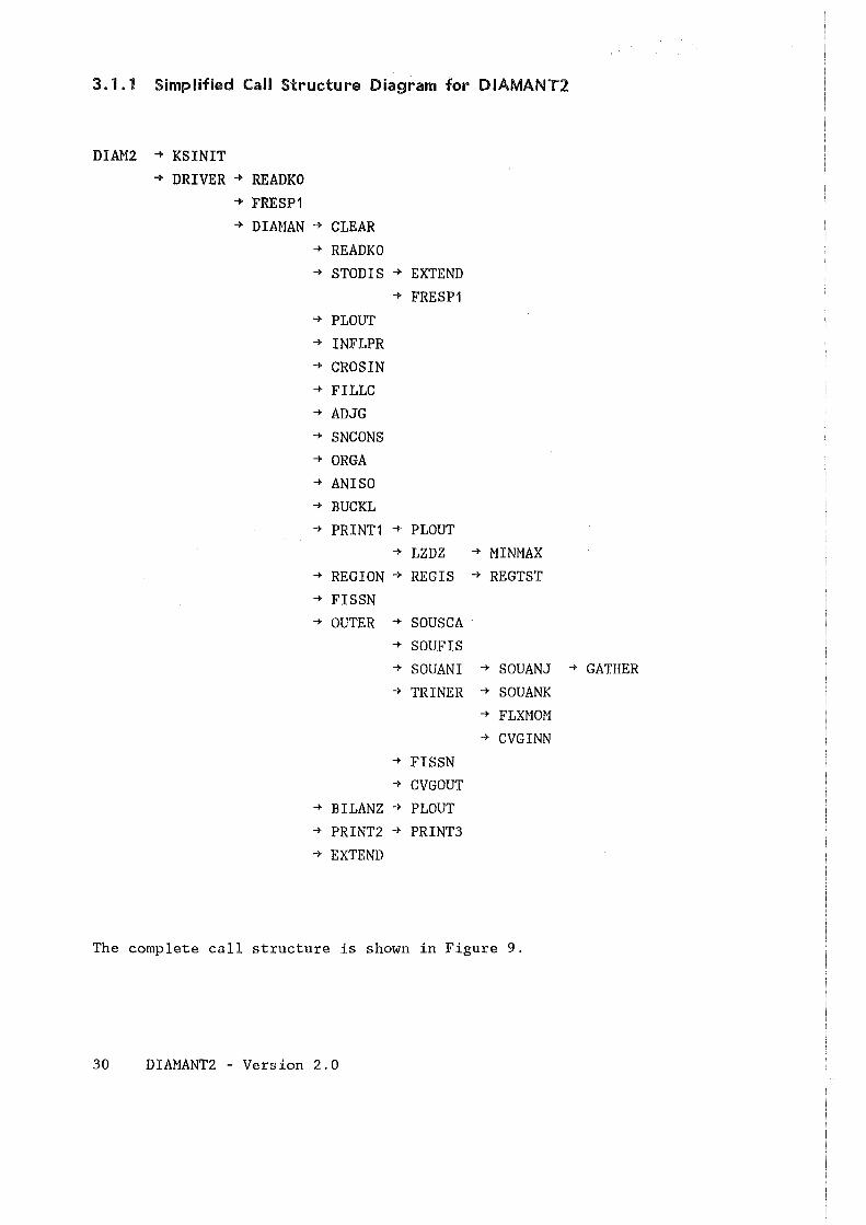
3. 1.1 Simplified Call Structure Diagram for DIAMANT2

DIAM2 -+ KSINIT -+ DRIVER -+ READKO

-+ FRESP1 -+ DIAMAN -+ CLEAR

-+ READKO -+ STODIS -+ EXTEND

-+ FRESP1 -+ PLOUT -+ INFLPR -+ CROSIN -+ FILLC -+ ADJG -+ SNCONS -+ ORGA -+ ANISO -+ BUCKL -+ PRINT1 -+ PLOUT

-+ LZDZ -+ MINMAX -+ REGION -+ REGIS -+ REGTST -+ FISSN -+ OUTER -+ SOUSCA

-+ SOUFIS -+ SOUANI -+ SOUANJ -+ GATHER -+ TRINER -+ SOUANK

-+ FLXHOM -+ CVGINN

-+ FISSN -+ CVGOUT

-+ BILANZ -+ PLOUT -+ PRINT2 -+ PRINT3 -+ EXTEND

The complete call structure is shown in Figure 9.


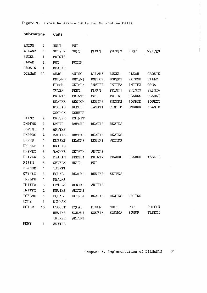
Figure 9. Cross Reference Table for Subroutine Calls

Subroutine Calls

AN ISO 2 MULT PUT BILANZ 6 GETFLX MULT PLOUT PUTFLX SUMT WRITKS BUCKL PRINTS CLEAR 2 PUT PUTIN CROSIN 1 READKR DIAMAN 44 ADJG ANISO BILANZ BUCKL CLEAR CROSIN

DMPFND DMPINI DMPPOS DMPWRT EXTEND FILLC FIS SN GETFLX INFLPR INITFA INITFX ORGA OUTER PERT PLOUT PRINT1 PRINT2 PRINT4 PRINTS PRINT6 PUT PUTIN READKC READKI READKR REGION REWIKS SNCONS SOUEND SOUEXT STODIS SUMUP TASKTI TIMLIM UNCHCK XSANIS XSCHCK XSHELP

DIAH2 2 DRIVER KSINIT DMPFND 4 DMPRD DMPSKP READKS RE\VIKS DMPINI 1 WRITKS DMPPOS 4 BACKKS DMPSKP READKS RE\VIKS DMPRD 4 DHPSKP READKS REWIKS WRITKS DMPSKP SKIPKS DMPWRT 3 BACKKS GETFLX WRITKS DRIVER 6 DIAMAN FRESP1 PRINT7 READKC READKO TASKTI FIS SN 3 GETFLX MULT PUT FLXMOH 1 TASKTI GETFLX 4 EQUAL READKS REWIKS SKIPKS INFLPR READKI INITFA 3 GETFLX REWIKS WRITKS INITFX 2 REWIKS WRITKS IOFLHO 5 EQUAL GETFLX READKS REWIKS WRITKS LZDZ HINMAX OUTER 13 CVGOUT EQUAL FIS SN MULT PUT PUTFLX

REWIKS SOU ANI SOUFIS SOUSCA SUMUP TASKTI

TRINER WRITKS PERT WRITKS


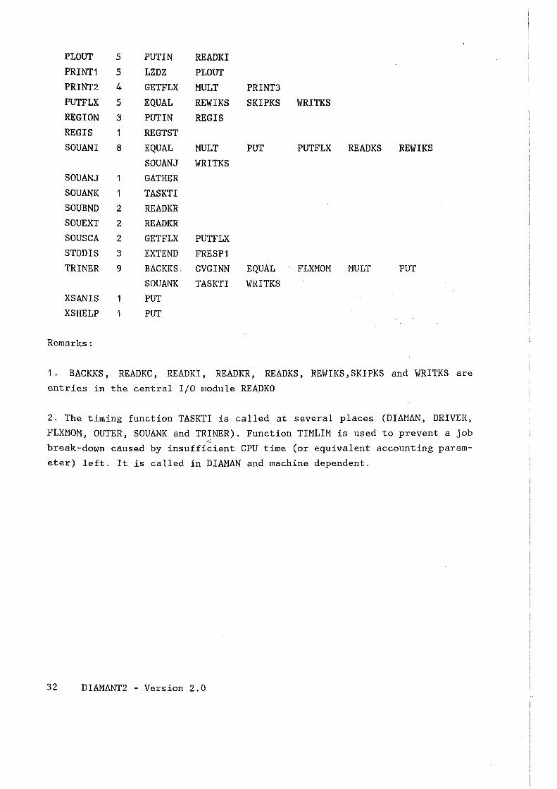
PLOUT 5 PUTIN READKI PRINT1 5 LZDZ PLOUT PRINT2 4 GETFLX MULT PRINT3 PUTFLX 5 EQUAL REWIKS SKIPKS WRITKS REGION 3 PUTIN REGIS REGIS 1 REGTST SOUANI 8 EQUAL HULT PUT PUTFLX READKS REWIKS

SOUANJ WRITKS SOUANJ GATHER SOUANK TASKTI SOUBND 2 READKR SOUEXT 2 READKR SOUS CA 2 GETFLX PUTFLX STODIS 3 EXTEND FRESP1 TRINER 9 BACKKS, CVGINN EQUAL FLXMOM NULT PUT

SOUANK TASKTI WRITKS XSANIS PUT XSHELP PUT

Remarks:

1 . BACKKS, READKC, READKI, READKR, READKS, REWIKS, SKIPKS and WRITKS are entries in the central I/0 module READKO

2. The timing function TASKTI is called at several places (DIAMAN, DRIVER, FLXNOM, OUTER, SOUANK and TRINER). Function TIMLIM is used to prevent a job break-down caused by insuffi~ient CPU time (or equivalent accounting parameter) left. It is called in DIANAN and machine dependent.


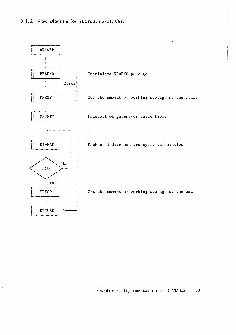
3.1.2 Flow Diagram for Subroutine:DRIVER

DRIVER


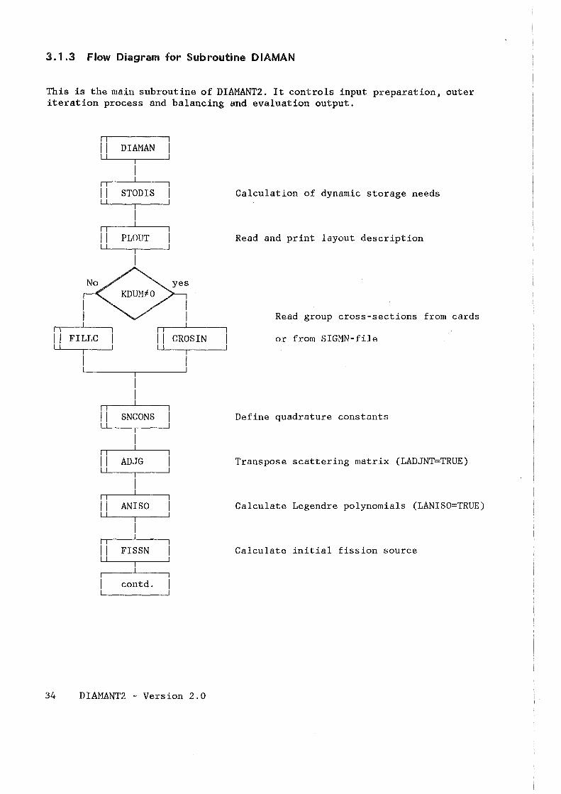
3.1.3 Flow Diagram for Subroutine DIAMAN

This is the main subroutine of DIAMANT2. It controls input preparation, outer iteration process and balancing and evaluation output.

II DIAHAN

II STODIS Calculation of dynamic storage needs

II PLOUT Read and print layout description

Read group cross-sections from cards

II FILLC II CROSIN or from SIGMN-file

II SNCONS Define quadrature constants

II ADJG Transpose scattering matrix (LADJNT=TRUE)

II ANISO Calculate Legendre polynomials (LANISO=TRUE)

II FISSN Calculate initial fission source

contd.

34 DIA1'1ANT2 - Version 2. 0

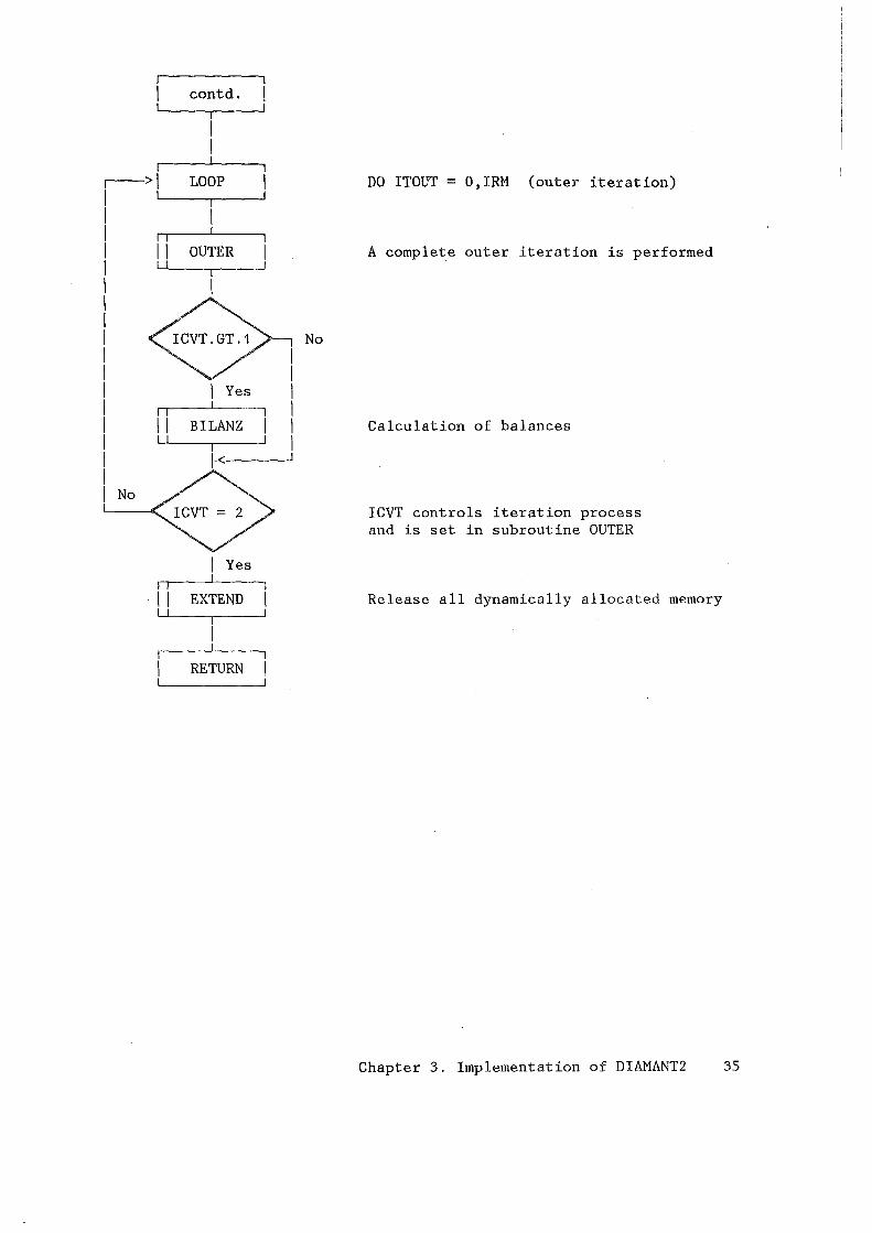
contd.

r-->1 LOOP DO ITOUT = O,IRM (outer iteration) I I I I II OUTER A complete outer iteration is performed I I I I I No I I I I Yes I I II BILANZ Calculation of balances I I I

~<

I ICVT controls iteration process and is set in subroutine OUTER

I Yes

II EXTEND Release all dynamically allocated memory

RETURN


3. 1.4 Flow Diagram for Subroutine OUTER

This subroutine performs one outer iteration.

OUTER

r->1 LOOP I I I I

II SOUSCA

1<-----'

II SOUFIS

II SOUANI II

1<.-----'

II TRINER

contd.

TRUE

FALSE

NO


DO IGCNT = 1,IGH Loop over energy groups

Calculation of isotropic in-scatter source

Calculation of group fission source

Calculation of anisotropic in-scattering source (for all moments k=0,1, ... ,ISCT)

Inner iteration for the group

Save scalar flux for group IGM

Save Legendre flux moments on file NFANI1

contd.

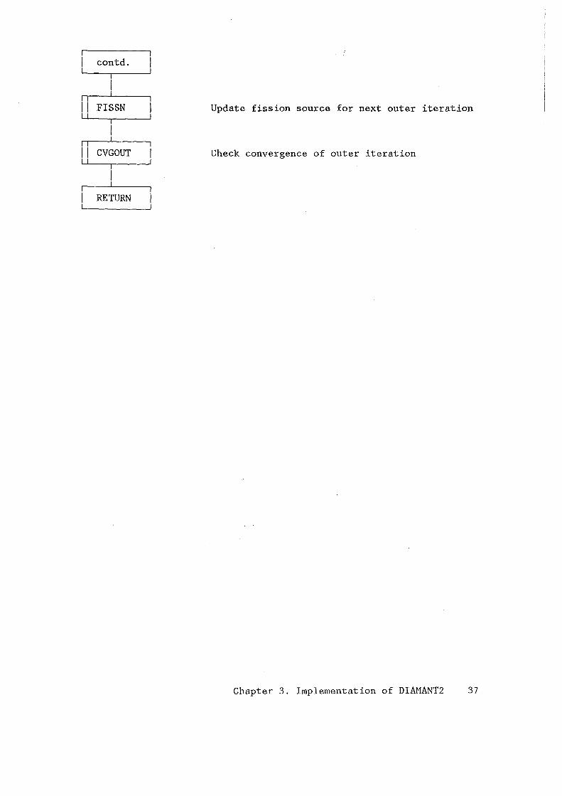
II FISSN Update fission source for next outer iteration

II CVGOUT Check convergence of outer iteration

RETURN


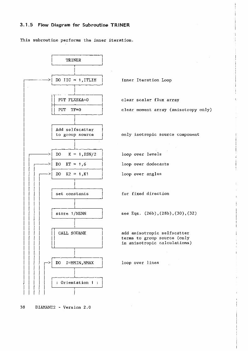
3. 1.5 Flow Diagram for Subroutine TRINER

This subroutine performs the inner iteration.

TRINER

>I DO IIC = 1, ITLHf Inner Iteration Loop I I I ~·

I II PUT FLXSKA=O clear scalar flux array I I II PUT TF=O clear moment array (anisotropy only) I I I I Add selfscatter I to group source only isotropic source component I I I I >I DO K = 1,ISN/2 loop over levels I I >I DO KT = 1 '6 loop over dodecants I I r-->1 DO K2 = 1 , K1 loop over angles I I I I I I I I I set constants for fixed direction I I I I I I I I I store 1/NENN see Eqs. (26b),(28b),(30),(32) I I I I I I I I II CALL SOUANK add anisotropic selfscatter I I II terms to group source (only I I II in anisotropic calculations) I I I I I I I I r>l DO I=MMIN,MMAX loop over lines I I I I I I I I I I I I I I I Grientation I I I I I I I I


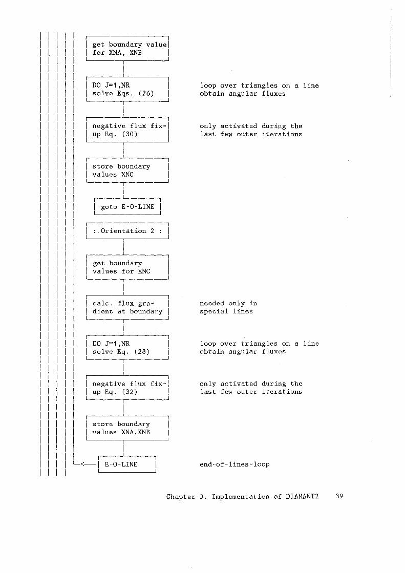
I I I I I I I get boundary valuel

I I I I I for XNA, XNB I I I I I I I I I I I I I I I I I I I I DO J=1 ,NR I loop over triangles on a line I I I I I solve Eqs. (26) I obtain angular fluxes I I I I L__ __J

I I I I I I I I I I I I negative flux fix-1 only activated during the I I I I up Eq. (30) I last few outer iterations I I I I I I I I I I I I I I I I store boundary I I I I values XNC I I I I I I I I I I I I I I I I goto E-0-LINE I I I I I I I I I I I I Grientation 2 I I I I I I I I I I I I I I I I get boundary I I I I values for XNC I I I I I I I I I I I I I I I I calc. flux gra- needed only in I I I I dient at boundary special lines I I I I I I I I I I I I I I I I DO J=1 ,NR loop over triangles on a line I I I I solve Eq. (28) obtain angular fluxes I I I I I I I I I I I I I I I I negative flux fix-1 only activated during the I I I I up Eq. (32) I last few outer iterations I I I I I I I I I I I I I I I I store boundary I I I I values XNA,XNB I I I I I I I I I I I I I I I L<-1 E-0-LINE end-of-lines-loop I I I

Chapter 3. Implementation of DIAHANT2 39

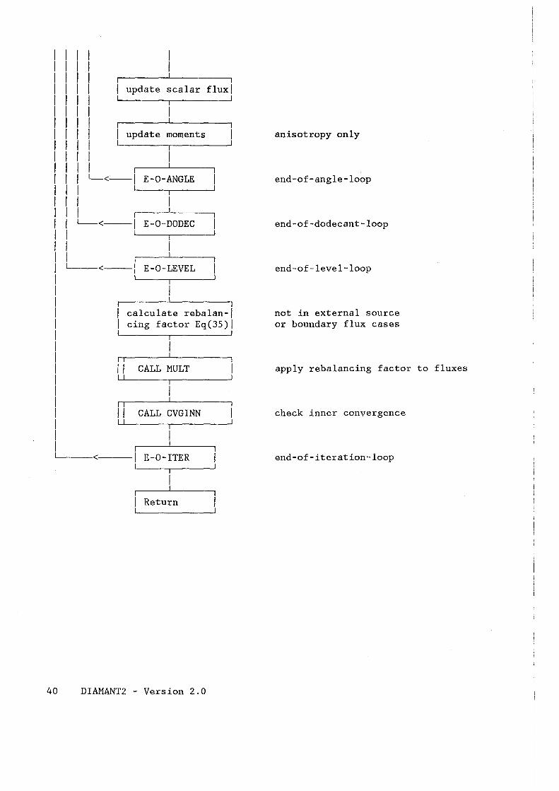
I I I I I I I I I I I I I I I I I I I I I I I I I I I I I I I I I I I I I I I I I I I I

I update scalar fluxl

update moments

I I I L_<--1 E-0-ANGLE I I I I I I 111 ~ ----, I I L__<--1 E-0-DODEC I I I I I I I I '----<--1 E-0-LEVEL I I I I I I I I I II I I I I II I I I

calculate rebalan-1 cing factor Eq(35)l

CALL NULT

CALL CVGINN

'-----<--- E-0-ITER

Return

40 DIANANT2 - Version 2.0

anisotropy only

end-of-angle-loop

end-of-dodecant-loop

end-of-level-loop

not in external source or boundary flux cases

apply rebalancing factor to fluxes

check inner convergence

end-of-iteration-loop

3.2 FUNCTION. OF THE DIFFERENT SUBROUTINES

In the following list, subroutines which contribute much to CPU time com

sumption are marked with (V), those which may also benefit from vectorization

are marked with (V/S). Only these few routines are worth tobe considered

when optimizing DIAMANT2 for a vector computer.

ADJG

AN ISO

BILANZ

BUCKL

CLEAR

CROSIN

CVGINN

CVGOUT

Transposes the scattering cross-section matrix for adjoint cal

culations

Calculates the spherical harmonics functions for use in aniso

tropic calculations

Calculates neutron balances and performs flux and source normal

ization

Adds a buckling correction term to total cross-section

Initializes arrays with 0.0 (V)

Reads cross-section input by card

Tests convergence of inner iterations (V)

Tests convergence of outer iterations (V/S)

D IAM2 Contains code abstract and calls DRIVER

DIAMAN Controls the total calculational sequence for one case

DMPFND Tries to find a restart dump on unit NFDMPO

DMP IN I Creates an end record on unit NFDMPN

DMPPOS Positions unit NFDMPN just before the end record to write out a

further restart dump

DMPRD Reads a restart dump

DMPSKP Skips one restart dump on unit NFDMPN

DMPWRT Writes a restart dump

DRIVER

EQUAL

FISSN

FLXMOM

GATHER

GETFLX

INFLPR

INITFA

INITFX

Controls the execution of a sequence of DIM1ANT2 calculations

Copies one array into another one (V)

Calculates the fission source (V/S)

Calculates anisotropic flux moments (V)

Gathers non-contiguous data into contiguous arrays (V)

Finds for a given group the flux of the previous outer iteration

Reads the group numbers for which fluxes are to be printed

Initializes the files NFANI1 and NFANI2 needed in anisotropic

calculations

Initializes the files NFSCR1 and NFSCR2 needed possibly as scratch

files


IOFLMO

LZDZ

Handles I/0 ef flux mements either en units NFANI1 and NFANI2 er

in COMMON bleck /COMMOM/

Sets up auxiliary arrays fer the mesh-angle sweeps during inner

iteratiens

MINMAX Finds the minimum and maximum limits ef the real medel in the

reference parallelegram

MULT Multiplicatien ef an ene-dimensienal array by a scalar (V)

ORGA Sets up the erganizatien ef the mesh-angle sweeps

OUTER Perferms ene euter iteratien

PERT Creates interface file fer perturbatien medule (file NFPERT)

PLOUT Input, interpretatien and printout of mixture distributien

POSMRT Prints relevant infermatien fer test purpeses and debugging

PRINTl

PRINT2

PRINT3

PRINT4

PRINT5

PRINT6

PRINT7

PUT

PUTIN

PUTFLX

REGION

REGIS

REGTST

SNCONS

SOUANI

(including COMMON blecks and arrays); see remark at the end ef this

list.

Tabulates some of the arrays specified by input cards

Tabulates fluxes and/or reaction rates or density tables according

to Eqs. (41) after convergence of iterations

Printing of flux values

Prints the external source input values

Prints the input buckling values

Prints input data cards in tabular form along with an explanation

Prints the PARAMETER values relevant for the code implementation

Initializes real arrays with a constant value (V)

Initializes integer arrays with a constant value (V)

Stores the flux for a given group in memory or on disk

Prints the region distribution and sets up array MIXREG

Used by subroutine REGION to determine contiguous mixture regions

Auxiliary routine used by REGIS

Defines the built-in SN-quadrature constants

Calculates the anisotropic group scattering source (subroutine

SOUANJ) and adds to this the group fission source contribution

during outer iterations

SOUANJ Calculates the anisotropic group scattering source excluding the

within-group scattering contribution (V/S) SOUANK Adds the anisotropic within-group scattering contribution to group

scattering source (during inner iterations) (V)

SOUBND Reads boundary flux input

SOUEXT Reads input data for external source cases

SOUFIS Calculates the fission source contribution to the group source

during outer iterations (V/S)


SOUSCA Calculates the scattering source contribution to the group source

during outer iterations (called only in isotropic calculations)

(V/S) STODIS Calculates the pointers to distribute working arrays A and 1\<l

SUMT Calculates the sum of two arrays (V)

SUMUP Sums up an array (FUNCTION) (V)

TRINER Performs the innex- iterations (V)

UNCHCK Checks the input FORTRAN unit numbers for consistency

XSANIS

XSCHCK

XSHELP

Remark:

Stores anisotropic within-group scatter cross section in array

X SANI

Campares the calculated absorption cross section with input value

Stores total, fission and within-group scatter cross section in

separate arrays

POSMRT is not called within the present implementation of DIAMANT2. But it

may be useful for debugging purposes to insert at suitable places calls to

this subroutine. POSMRT prints out the values of all COMMON variables (as

namelists) as well as the contents of the different code arrays. POSMRT has

no parameter list an the call. If called without modification and especially

within inner iterations, this routine may produce a huge amount of output!

POSMRT itself calls a couple of auxiliary subroutines which are not included

in the above list (but are provided along with the source deck).

Subroutines with different implementation for STAND-ALONE and KAPROS

version or on different computers

EXTEND Performs dynamic field extensions and releases (see 11 Use as

Stand-alone program 11 an page 71). FILLC

FRESP1

JTIME

KSCC

Gets cross-section data from a SIGMN-block (see 11 Use as Stand-al

one program" an page 71).

Determines the amount of memory space available for array exten

sions (see "Use as Stand-alone program" on page 71).

Supplies the remaining CPU time for the job (system dependent) (see 11Use as Stand-alone program11 an page 71).

Sets a stop code in case of any error condition during execution

(see 11Use as Stand-alone program11 an page 71).


KSINIT Sets channel numbers for standard read and print units (see "Use

as Stand-alone program" on page 71).

READKO Central I/0 module for binary data transfers (see "Use as Stand-

alone program" on page 71).

TASKTI Function; returns the CPU time already used in seconds

TIMLIM Function; returns the CPU time still left in seconds (or some

equivalent resource control parameter)

Additional subroutines for KAPROS version

OB LENG

FILSET

FIL TES

FILTRA

INITDB

KS ....

WQRG

Gets the length of KAPROS data blocks

Auxiliary program to FILLC to initialize arrays

Auxiliary program to FILLC to test input

Performs the transport correction on total cross-section

Initializes new kAFiWS data blocks (beloiigs to READKO package)

All these subroutines belang to the KAPROS system kernel

Reading of KAPROS SIGMN blocks or specified parts of them


3.3 DATA MANAGEMENT, COMMON USAGE AND DATA FILES

In the following we describe data management and data files as used in the

stand-alone version. Differences necessary for the KAPROS version are

described in "KAPROS Implementation" on page 69. For an implementation of

DIAMANT2 one has to select PARMiETER values activating or deactivating

options, defining dimensions and setting certain maximum values. As these

values depend on the computer used, we postpone a discussion of them (see

"How to Choose PARAMETER Values" on page 86).

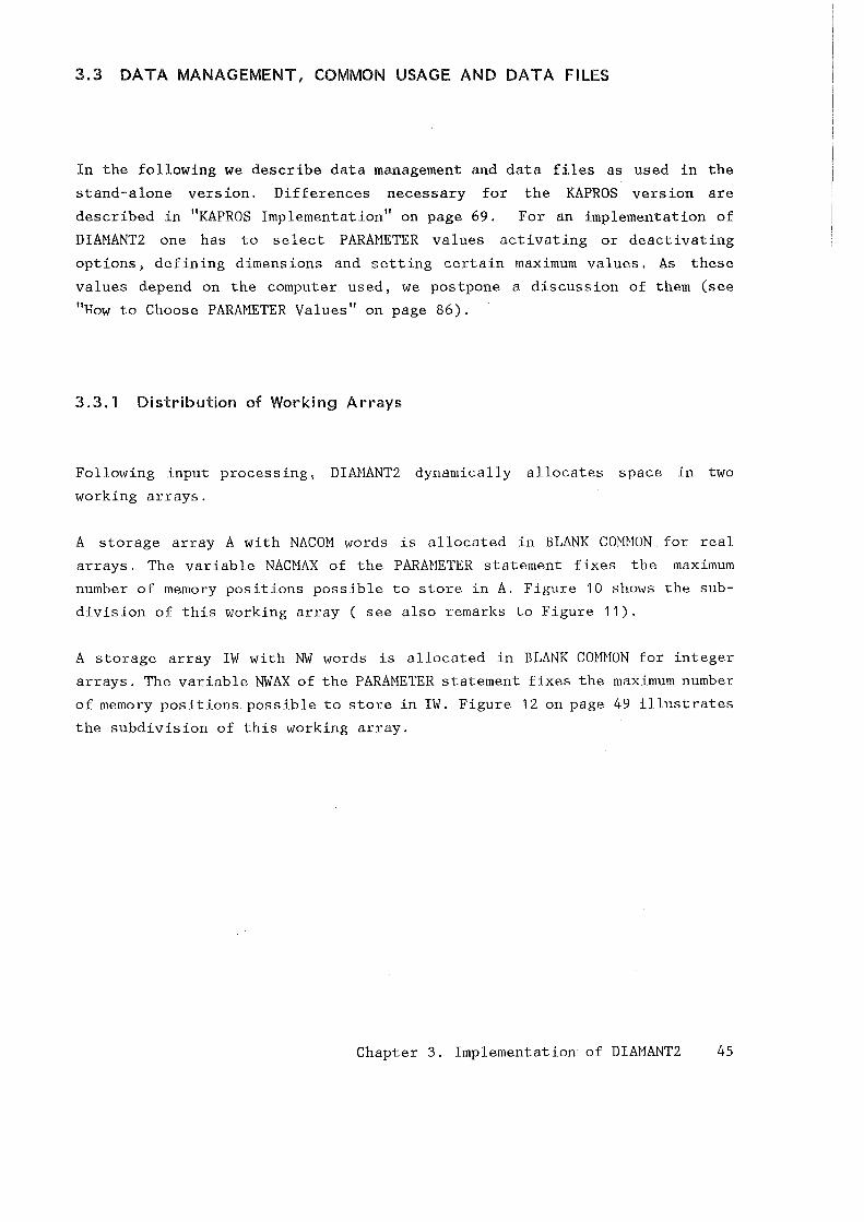
3.3. 1 Distribution of Working Arrays

Following input processing, DIAHANT2 dynamically allocates space in two

working arrays.

A storage array A with NACOM words is allocated in BLANK COHHON for real

arrays. The variable NACNAX of the PARMIETER statement fixes the maximum

number of memory positions possible to store in A. Figure 10 shows the Sub

division of this working array ( seealso remarks to Figure 11).

A storage array IW with NW words is allocated in BLANK COHHON for integer

arrays. The variable NWAX of the PARMiETER statement fixes the maximum number

of memory positions possible tostorein IW. Figure 12 on page 49 illustrates

the subdivision of this working array.


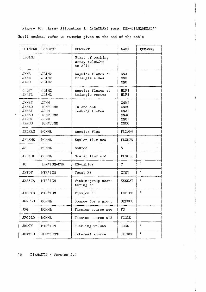
Figure 10. Array Allocation in A(NACNAX) resp. DBN=DIAN2f>REAL~~4

Small numbers refer to remarks given at the end of the table

POINTER! LENGTH 1

JPOINT

JXNA JXNB JXNC

JHLP1 JHLP2

I JXNBI I JXNBO I JXNAI

·I JXNAO I JXNCI I JXNCO

I JFLXAN

JFLXNE

JS

JFLXOL

JC

JXTOT

JLH12 JLIN2 JLIN2

JLnt2 JLIH2

JJH~t

IGN~'~JJHH

JJHH IGW~JJH~t

JJN~t

IGH~'~JJHN

NCHHL

HCHHL

HCNNL

NCmtL

JXSSCA HTR~~IGN

JXSFIS NTR~'(IGN

JGRPSO HCHHL

JFG MCNHL

JFGOLD MCHHL

JBUCK HTR~~IGH

JEXTSO IGM~'>"MCMML

CONTE NT

Start of working array relative to A(1)

Angular fluxes at triangle sides

Angular fluxes at triangle vertex

In and out leaking fluxes

Angular flux

Scalar flux new

Source

Scalar flux old

XS-tables

Total XS

Within-group scattering XS

Fission XS

Source for a group

Fission source new

Fission source old

Buckling values

External source

46 DIAHANT2 - Version 2.0

NAHE

XNA XNB XNC

HLP1 HLP2

XNBI XNBO XNAI XNAO XNCI XNCO

FLXANG

FLXNEW

s

FLXOLD

RENARKS

c I 5

XTOT I 5

XSSCAT I 5

I

XSFISS I 5

GRPSOU I

FG

FGOLD

BUCK I 2

EXTSOU I 2

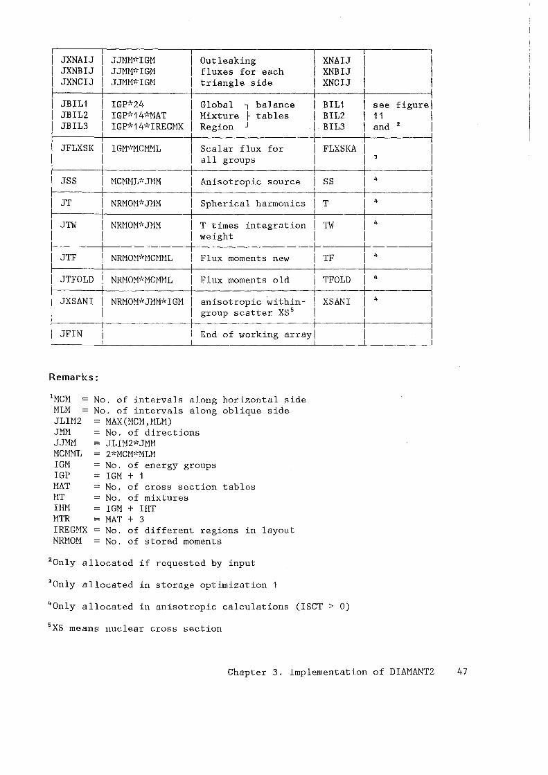
JXNAIJ JJHW,.IGM Outleaking JXNBIJ JJHW,.IGM fluxes for each JXNCIJ JJMM~"IGH triangle side

JBIL1 IGP~"24 Global l balance JBIL2 IGP~"14~'cHAT Mixture ~ tables JBIL3 IGP~"14~'ciREGHX Region J

JFLXSK IGM~I-HCMHL Scalar flux for all groups

JSS MCMNL~'; JHM Anisotropie source

JT NRMON~"JHM Spherical harmonics

JTW NRHOW,.JHH T times integration weight

JTF NRHOW"MCHML Flux moments new

JTFOLD NRHOW"MCMML Flux moments old

JXSANI NRHOM~'"JMM~'•IGM anisotropic ~ithin-group scatter XS 5

JFIN End of working arrayl

Remarks:

1 MCH = MLH = JLIN2 JMM JJMM MCMML IGM IGP MAT MT IHM MTR IREGMX NRMOM

No. of intervals along horizontal side No. of intervals along oblique side = MAX(MCM,MLM) = No. of directions = JLU12~'• JMM = 2~1-MCW•MLM = No. of energy groups = IGM + 1 = No. of cross section = No. of mixtures = IGM + IHT = MAT + 3

tables

= No. of different regions in = No. of stored moments

layout

2 0nly allocated if requested by input

3 0nly allocated in storage optimization

XNAIJ XNBIJ XNCIJ

BIL1 BIL2 BIL3.

FLXSKA

ss

T

TW

TF

TFOLD

X SANI

4 0nly allocated in anisotropic calculations (ISCT > 0)

5 XS means nuclear cross section

see figurel 11 I and 2 I

I I 3

I

I 4

I 4

I 4

I

I 4

I 4

I 4

I


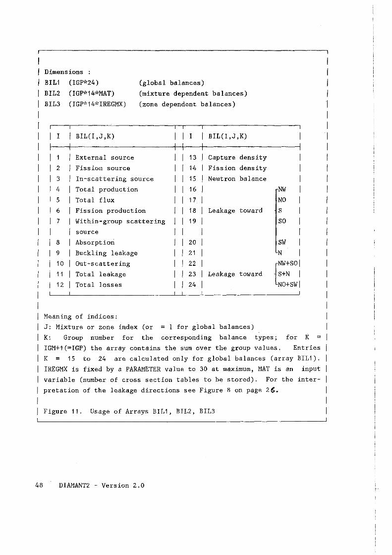
I I Dimensions :

I I I I I I I I I I I I I I I I I I I I I I I I I I I I I I I I

BIL1

BIL2

BIL3

I

2

3

4

5

6

7

8

9

10

11

12

(global balances)

(IGP*14~'rMAT)

( IGP~'r14,'riREGMX) (mixture dependent balances)

(zone dependent balances)

BIL(I ,J ,K)

External source

Fission source

In-scattering source

Total production

Total flux

Fission production

Within-group scattering

source

Absorption

Buckling leakage

Out-scattering

Total leakage

Total lasses

I I I

I I I I I I I I I I I I I I I I I I I I I I I I I I

13

14

15

16

17

18

19

20

21

22

23

24

BIL(I ,J ,K)

Capture density

Fission density

Neutron balance

Leakage toward

Leakage toward

Meaning of indices:

J: Mixture or zone index (or = 1 for global balances)

NW

NO

s so

sw N

{NW+SO S+N

NO+SW

K: Group number for the corresponding balance types; for K =

IGM+1(=IGP) the array contains the sumover the group values. Entries

K = 15 to 24 are calculated only for global balances (array BIL1).

IREGMX is fixed by a PARAMETER value to 30 at maximum, MAT is an input

variable (number of cross section tables tobe stored). For the inter

pretation of the leakage directions see Figure 8 on page 26.

Figure 11. Usage of Arrays BIL1, BIL2, BIL3


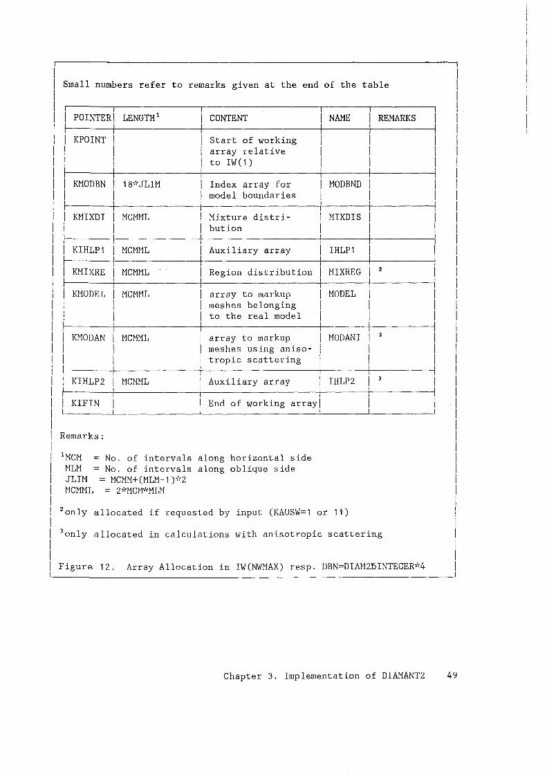
I I I Small numbers refer to remarks given at the end of the table I I I I I I I POINTER I LENGTH 1 CONTE NT NAME RE MARKS I I I I KPOINT Start of working I I array relative I I to IW(1) I I I I KMODBN 18~'(JLIM Index array for MODBND I I model boundaries I I I I KMIXDI MCMML Mixture distri- MIXDIS I I bution I I I I KIHLP1 MCMML Auxiliary array IHLP1 I I I I KMIXRE ~1CMML Region distribution ~1IXREG I 2 I I I I KMODEL MCMML array to markup MODEL I I meshes belanging I I to the real model I I I I KMODAN MCMML array to markup MODANI I 3 I I meshes using aniso- I I I tropic scattering I I I I I KIHLP2 MCMML Auxiliary array IHLP2 I 3 I I I I KIF IN End of working arrayl I I I I I I Remarks: I I I I 1 MCM = No. of intervals along horizontal side I I MLM = No. of intervals along oblique side I I JLIM = MCMM+(MLM-1)*2 I I MCMML = 2~'(MCM~'(MLM I I I I 2 only allocated if requested by input (KAUSW=1 or 11) I I I I 3 only allocated in calculations with anisotropic scattering I I I I I I Figure 12. Array Allocation in IW (NWMAX) resp. DBN=DIAM2lSINTEGER;'(4 I


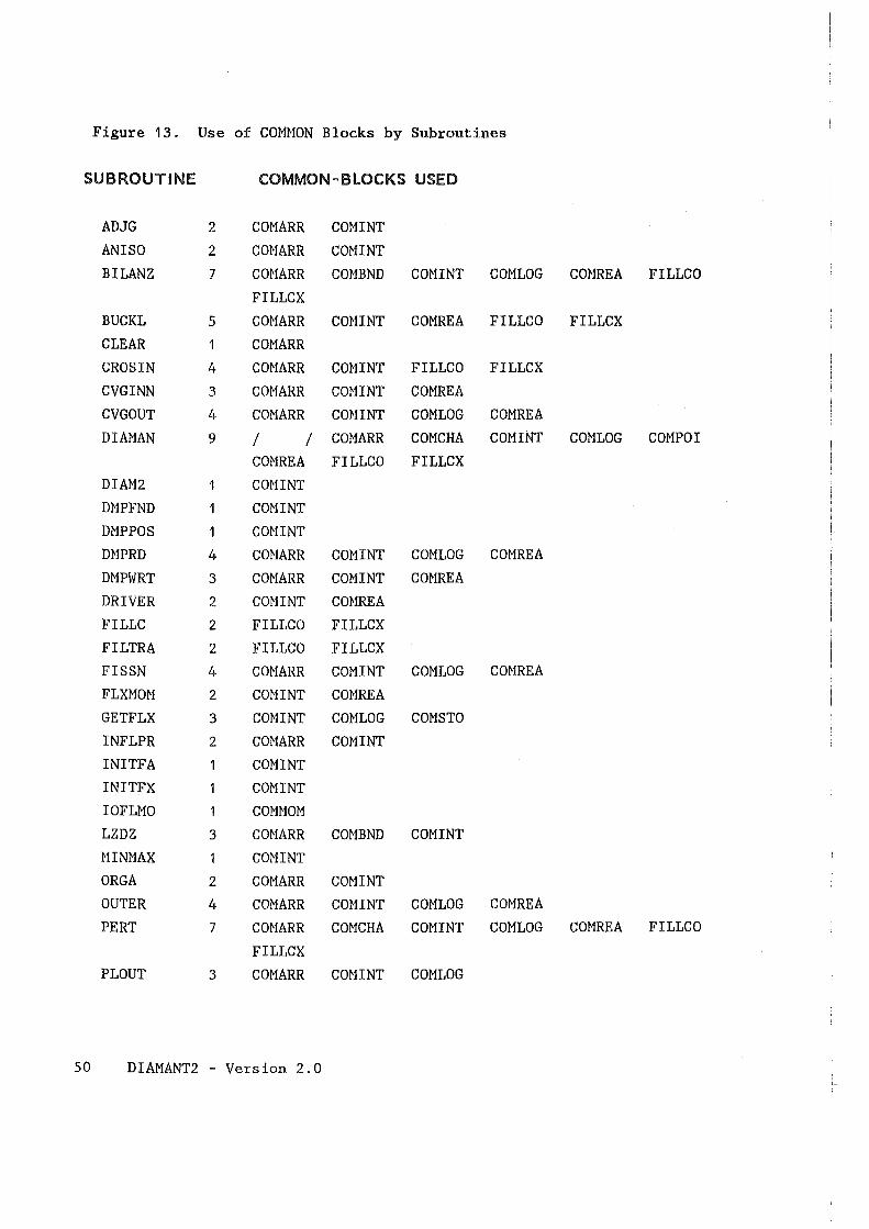
Figure 13. Use of COMMON Blocks by Subroutines

SUBROUTINE COMMON-BLOCKS USED

ADJG 2 COMARR COMINT AN ISO 2 COMARR COHINT BILANZ 7 CO HARR COMBND CO NI NT COMLOG COMREA FILLCO

FILLCX BUCKL 5 COMARR COHINT COMREA FILLCO FILLCX CLEAR 1 COMARR CROSIN 4 COMARR COMINT FILLCO FILLCX CVGINN 3 COMARR COMINT COMREA CVGOUT 4 COMARR COHINT COMLOG COMREA DIAMAN 9 I I CO HARR COMCHA COMINT COMLOG COMPOI

COMREA FILLCO FILLCX DIAM2 cmnNT DMPFND COMINT DMPPOS 1 cmnNT DMPRD 4 COMARR COMINT COMLOG COMREA DMPWRT 3 COMARR COMINT COMREA DRIVER 2 CONINT COMREA FILLC 2 FILLCO FILLCX FILTRA 2 FILLCO FILLCX FIS SN 4 CO NARR COMINT COMLOG COMREA FLXMOM 2 COMINT COMREA GETFLX 3 COMINT COMLOG COMSTO INFLPR 2 COMARR COMINT INITFA COMINT INITFX COMINT IOFLMO COMMOM LZDZ 3 COMARR CO MB ND COMINT MINMAX 1 COMINT ORGA 2 COMARR COMINT OUTER 4 COMARR COMINT COMLOG COMREA PERT 7 COMARR COMCHA CO MINT COMLOG COMREA FILLCO

FILLCX PLOUT 3 COMARR COMINT COMLOG


SUBROUTINE COMMON-BLOCKS USED

PRINT1 5 COMARR COHINT COHREA FILLCO FILLCX PRINT2 6 COMARR COMINT COHLOG COMREA FILLCO FILLCX PRINT3 COMINT PRINT4 COMINT PRINTS COMINT PRINT6 3 CONCHA COHINT COHREA PUTFLX 3 CONINT COHLOG COHSTO REGION 1 COMINT RE GIS COMINT REGTST cmHNT SNCONS 2 COMARR COHINT SOU ANI 3 COMINT COMLOG COMREA SOUANJ 3 CO HARR COMINT COMREA SOUANK 3 cmnNT COMLOG COMREA SOUEND 4 CO HARR COMBND COMINT COMLOG SOUEXT cmnNT SOUFIS 3 COMINT COMLOG COMREA SOUSCA 2 COMINT COMREA STODIS 5 I I COMARR COHINT COMLOG COMPOI

TRINER 5 Cm1ARR COMBND COMINT COMLOG COMREA

UNCHCK COMINT XSANIS 3 COMARR cmnNT COMREA XSCHCK 2 COHINT COHREA XSHELP 2 COMARR COMINT


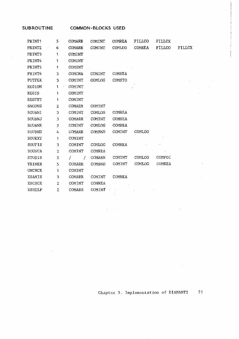
3.3.2 Use of COMMON Blocks

DIAMANT2 currently uses 11 named COMMON blocks: /COMARR/, /CONBND/, /COM

CHA/, /COMINT/, /COMLOG/, /CONMOM/, /COMPOI/, /COMREA/, /COMSTO/, /FILLCO/,

/FILLCX/ and a BLANK COMMON / j.

Use of the different COMMON blocks by the various subroutines is shown in

Figure 13 on page 50. This table has been produced by the utility OBJXREF

/12/. Usage of the variables in different COMMON blocks by subroutines is

shown in Figures 14 to 21. These tables have been generated using the static

analyzer module of the test system RXVP /13/. The following list gives a

short characterization of the function of the different COMMON blocks.

ICOMARRI

ICOMBNDI

ICOMCHAI

ICOMINTI

ICOMLOGI

ICOMMOMI

ICOMPOII

ICOMREAI

ICOMSTOI

IFILLCOI

IFILLCXI

I I

contains arrays dimensioned by a PARMIETER statement

contains some arrays needed to organize the mesh-angle sweeps

stores the 60 characters specifying the run identification

stores scalar control integers

stores logical switches

contains the working array used to replace external storage of

anisotropic flux moments if space is sufficient; it is used

exclusively by subroutine IOFLNO.

pointers identifying subarrays in the working arrays A, IW

stores scalar real variables

stores the number of words allocated in working arrays and an

array used to optimize I/0 in GETFLUX/PUTFLUX

stores pointers to special cross section types and some auxil

iary integers

stores the sequence of cross section type names

contains the working arrays A ,IW and their maximum lengths


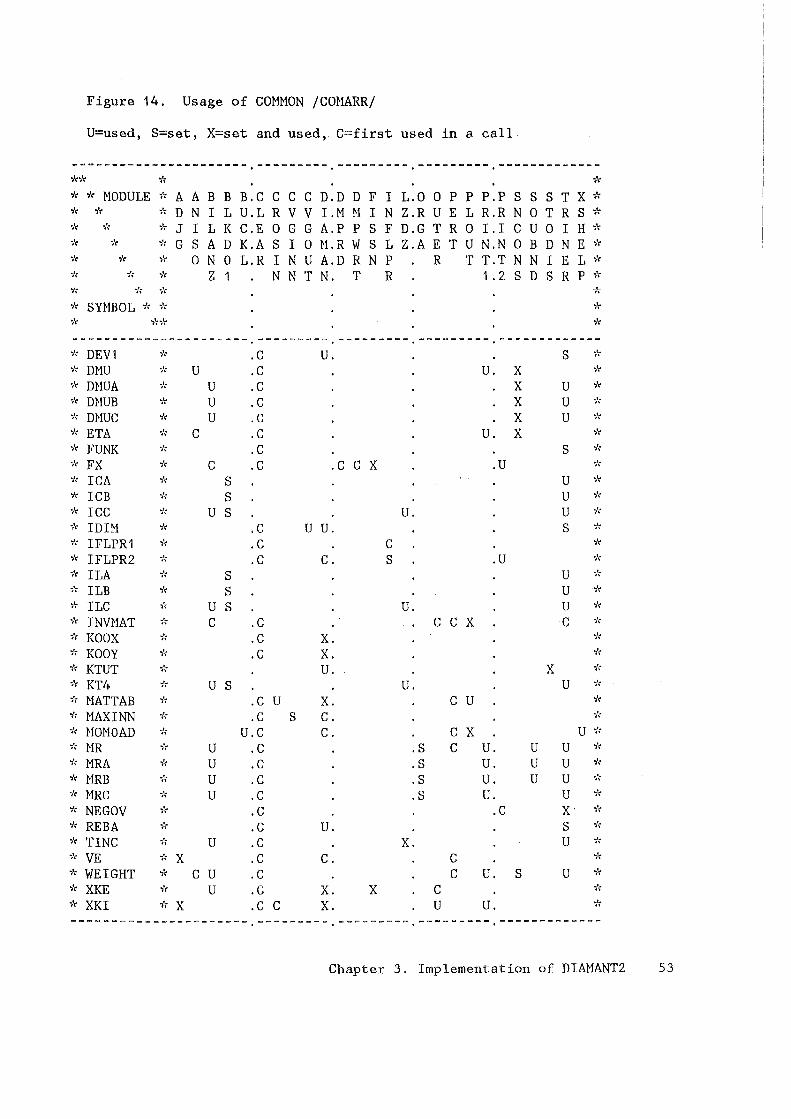
Figure 14. Usage of COMMON /COMARR/

U=used, S=set, X=set and used, C=first used in a call

---------------------- --------- --------- --------- -------------")'("#~ ~'( ;'(

-;'( 'i'( NODULE i't A A B B B.C c c c D.D D F I 1.0 0 p p P.P s s s T X 'i'(

-;'( i'l ;'t D N I L U.L R V V I.M H I N Z.R u E L R.R N 0 T R s "'k ;'( ~'t i': J I L K C.E 0 G G A.P p s F D.G T R 0 I. I c u 0 I H i't

;'-( ··;', i't G s A D K.A s I 0 H.R w s L Z.A E T u N.N 0 B D N E .... 'i't ·k 'i't 0 N 0 L.R I N u A.D R N p R T T.T N N I E L .... "'k ;'~ ;'t z 1 N N T N. T R 1 . 2 s D s R p ;'(

;'( 'i'~ ;'t .. .. 'f'r SYMBOL '1: ;'( 'i't

'i't ;','i't 'i't

---------------------- --------- --------- --------- -------------;': DEV1 'i't . c u . s ;'r ..,., DMU ;'( u . c u . X ";'\

.. k DHUA i't u .c X u .... •k DHUB .... u .c X u ;'t

.. k DMUC ';1\ u .c X u .,.,

"'/( ETA l't c . c u . X ··~ 'i't FUNK .... .c s ;'t

•k FX ;'( c .c .c c X .u ;':

'i't ICA ..,., s u i't

;'t ICB i't s u ';'(

'i't ICC .,., u s u. u ""k

t't IDIM ;'t .c u u. s "i't

;': IFLPR1 ;'t .c c ;'t

;'t IFLPR2 ··): .c c. s .u "k

;'t ILA ;': s u ;'\

*'' ILB 'i't s u ;'t

'"k ILC •k u s u. u ;'t

;'t INVHAT ""k c .c c c X c '"k

""k KOOX "'k .c X. •k

'i't KOOY ..,., .c X. ";'(

i't KTUT 'i't u. X ;'t

o.)( KT4 ;'( u s u. u ..,.,

•k MATT AB ""/( .c u X. c u i't .. ,., MAXINN •;'( .c s c. ';'(

i't HOHOAD i'( u.c c. c X u 'f'(

'i't ~1R i'( u .c .s c u. u u ';'(

"k MRA .... u .c .s u . u u ;'t

;'t MRB i't u .c .s u. u u 'i'(

..,., MRC ;'t u .c .s u. u .... 'i't NE GOV "'/( .c .c x· '"k

'i't REBA 't'r . c u . s ;'(

i'( TINC ;'t u .c X. u ;'t

i't VE ;': X .c c. c 'i't

;'t WEIGHT 'i't c u . c c u . s u .. .. ..,., XKE o./( u . c X . X ro i't u

'i't XKI .... X .c c X. u u. ';'(

---------------------- --------- --------- --------- -------------


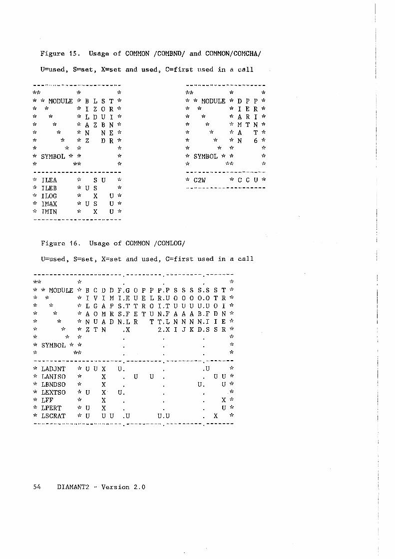
Figure 15. Usage of COMMON /COMBND/ and COMMON/COMCHA/


*"'~'c * ;': ;h'f ,'f ;'f

.,~: .,,~ MODULE ;'r B L s T "';'( ;'r * MODULE "'i'r D p p ;'t

;'f 'i'r ;'r I z 0 R o;'( 'i'r ;'f -;'r I E R * ;'r 'i'r ";'; L D u I ;'r * * * A R I -;'(

"i'r * ;'f A z B N 'i': ;'r -;'( 'i'r M T N ;'r

";'; "i'r * N N E -;'( 'f'r 'i'r ;'( A T ;':

't'r * ;'f z D R ;'f * -;'( ;'r N 6 'f'r

;'r ;'r "f'f "i'r ;'r * "i'r ;'r

;'; SYMBOL ;'r * 'i'r ";'( SYMBOL "i'r ;'r ;'f

* ** "1: ""

"i'r't'( ;'r

---------------------- --------------------;'( ILEA ;'-; s u * ";'; C2W ;'r c c u ;'f

.. k ILEB ;'r u s ;'t --------------------'t'r ILOG ';'; X u "i':

;'f IHAX ;': u s u * "'i'( IHIN i'( X u ;'r

Figure 16. Usage of COMMON /COMLOG/


---------.---------.-------•r •r MODULE •r B C D D F. G 0 P P P. P S S S S . S S T •r * * *I V IM I.E U E L R.U 0 0 0 0.0 T R * * * * L GAP S.T T R 0 I.T U U U U.U 0 I * * * * A 0 M R S.F E TU N.F A A A B.F D N * * * * N U A D N.L R T T.L N N N N.I I E * * * * Z T N .X 2.X I J K D.S S R *

---------------------- ................................... --------- -------"i'r LADJNT -;': u u X u. .u "i'r

-1: LANISO ;'t X u u u u ;'r

;'( LBNDSO "i'( X u. u "i'r

;': LEXTSO "'i~ u X u. ;'t .,,, LFF ;'t X X 'i'\

'i'r LPERT ..,,, u X u -Ir

;'( LSCRAT ;'t u u u .u u.u X ;'t

---------------------- --------- --------- -------. . .


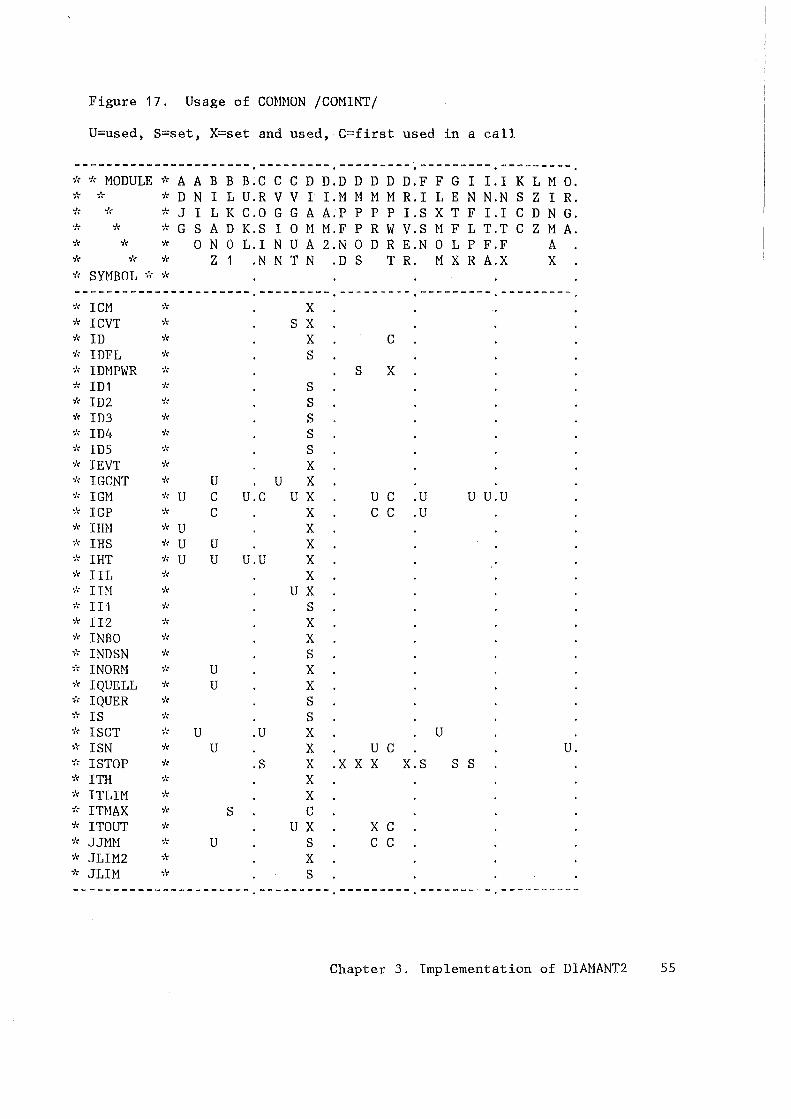
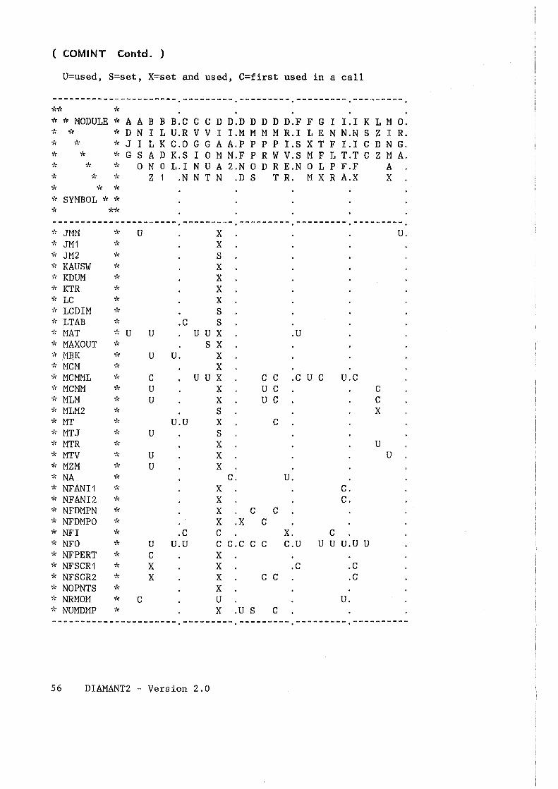
Figure 17. Usage of COMMON /COMINT/


---------------------- ---------.-----~---~---------.---------;'( ;'( MODULE ;'( A A B B B . C C C D D. D D D D D . F F G I I . I K L N 0. * * * D N I L U.R V V I I.M M M M R.I L E N N.N S Z I R. * * * J I L K C.O G GA A.P PP P I.S X T F I.I CD N G. * * * G S A D K.S I 0 M M.F P R W V.S M F L T.T C Z M A. * * * 0 N 0 L.I NU A 2.N 0 D R E.N 0 L P F.F A * * * Z 1 .N N T N .D S T R. N X R A.X X .,, SYMBOL ;'( ;'(

---------------------- --------- ""'""'"'""""'""'""'""'"""= ."..,. ... ...,.,....,..,. __ ---------

•#'( ICM 'i': X i't ICVT 'i~ s X '"J't ID 'i'\ X c ..,., IDFL 'i'r s ..,., IDHPWR ;'r s X .. /( ID1 ;'( s ·k ID2 "'k s ;'( ID3 t;'r s ";'( ID4 i't s i'r ID5 ;': s ·k IEVT 'i'r X i'( IGCNT ;'( u u X •k IGM '"k u c u.c u X u c .u u u.u .,., IGP ;'r c X c c .u ;'r IHN .. k u X ·;'( IHS ;': u u X ··k IHT 'i'( u u u.u X "k IIL 'i'( X •k IH1 ;"( u X ;~ .. II1 ;'r s i'r II2 i'r X i't INBO 'I'( X ;'( I ND SN ;'r s i'r INORf>1 'i'r u X i'\ I QUELL i'r u X ·k I QUER i'r s 'i'r IS ;'r s "'k ISCT 'i'r u .u X u •k ISN 'i'r u X u c u. ..,., ISTOP ;'r .s X .X X X x.s s s 'i'r ITH ·k X ;': I TL IM i'r X i'\ ITHAX •k s c "i'r ITOUT ;'r u X X c ";'\ JJMH 'i'r u s c c ..,,, JLIM2 ;'r X ;'( JLIM ;'r s ---------------------- --------- --------- ------~== ~---------. . . .


( COMINT Contd. )


====------------------ --------- --------- --------- ---------~'r* * * * MODULE ~'r A A B B B.C c c D D.D D D D D.F F G I I. I K L M 0. ";~ ~'( ";'( D N I L U.R V V I I.M M M M R.I L E N N.N s z I R. ";'( ~'r ~'( J I L K c.o G G A A.P p p p I.S X T F I. I c D N G. ,'r ,'r "f'r G s A D K.S I 0 M M.F p R w v.s H F L T.T c z H A. ?'r ~'r ..,., 0 N 0 L. I N u A 2.N 0 D R E.N 0 L p F.F A ";'( ";'( "('( z 1 .N N T N .D s T R. M X R A.X X ~'r -;'( ,'(

'i'~ SYMBOL -;'( ";'(

";'( -;'(";'(

---------------------- --------- --------- --------- ---------"k JMM ,~r u X u. ";'( JM1 ... , X ";'\ JM2 "'~'' s 'i'r KAUSW 'i'r X ;': KDUM o;': X 'i': KTR ,'( X ";'( LC 'i'r X

"'" LCDIM 'i': s ";'( LTAB i': .c s ;': HAT ,'r u u u u X .u ..,., MAXOUT -;'r s X •k H~K ,'( u u. X ,'( MCM t': X 'i'l MCMML ..,., c u u X c c .c u c u.c ;'( MCMM ";" u X u c c -;': ~fLM 'i'( u X u c c ··k MLM2 'i': s X •k MT 'i'r u.u X c ~k MTJ t'r u s 'i': MTR ,'( X u "'k MTV ,'( u X u "k MZM ";'( u X ,'r NA ,'r c. u. ,'( NFANI1 ,'r X c. "i': NFANI2 o;'r X c. 'i'r NFDMPN ";'( X c c * NFDMPO ";': X .X c 't( NFI ,'r .c c X. c ,'r NFO ";': u u.u c c.c c c c.u u u u.u u ,'( NFPERT ,'( c X ";'( NFSCR1 'i': X X .c .c "'k NFSCR2 * X X c c .c * NOPNTS i'r X ,'( NRMOM ,'( c u u. ;'( NUMDMP ,.( X .u s c ----------------·-----.---------.---------.---------.----------


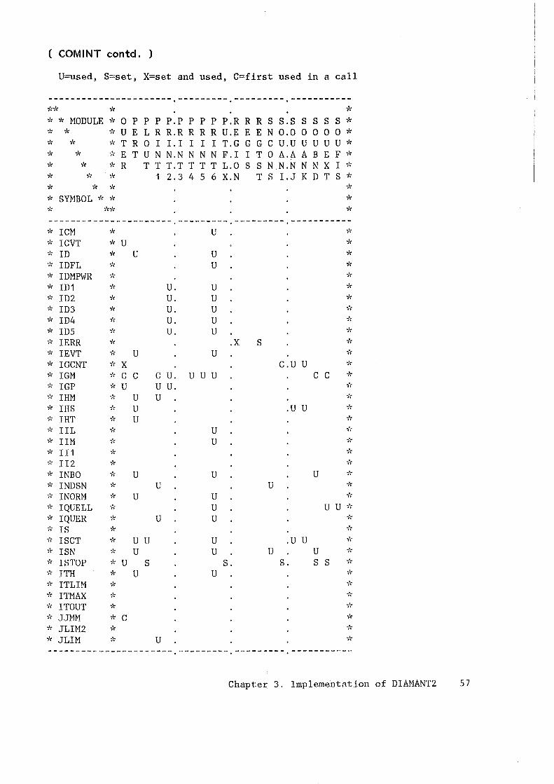
( COMINT contd. )


---------------------- --------- --------- -----------*";~ * ~'(

-;': ~'( MODULE ~'( 0 p p p P.P p p p P.R R R s s.s s s s s ~'(

o;': ~'( * u E L R R.R R R R U.E E E N 0.0 0 0 0 0 ,'(

~'; ~'; ~'( T R 0 I I. I I I I T.G G G c u.u u u u u -;': .. /, ;'-( * E T u N N.N N N N F. I I T 0 A.A A B E F ~';

•k ~'; ;'-( R T T T.T T T T L.O s s N N.N N N X I ;'\

;'\ ";'( ~'( 1 2.3 4 5 6 X.N T s I.J K D T s * * ;': ;'( i~

·k SYMBOL -;'( ";'\ •;'\

~'; -;'r;'( ;'-(

---------------------- --------- --------- -----------··k ICM ~'; u ..,~.;

•k ICVT ";'-( u -;'-(

'" ID ";'; u u ;'-(

..,,, IDFL ;'( u ;';

;': IDMPWR * ~';

;': ID1 ";': u. u ;':

;'-( ID2 "'-/\ u. u ;':

'"k ID3 ~'; u. u ;':

;': ID4 ~'; u. u ;':

;': IDS -;': u. u ;'-(

;': IERR -;'( .X s --;':

;'( IEVT ;'\ u u i'\

-;': IGCNT ;'( X c.u u ;'(

";'( IGM ;': c c c u. u u u c c '"k

;'; IGP ..,,, u u u. '"k

'i': IHM ;'; u u ~';

7: IHS ;'-( u .u u ;'\

;': IHT t': u 'i':

;': IIL ';'\ u 'i't

.. k IIM t': u '"k

;': II1 ;': 'i':

"'k II2 ;': ;'r

~'; INBO ;'\ u u u •·k

;': I ND SN 'i': u u 'i't

;': I NORM t': u u 'i'\

;': I QUELL ;'-( u u u ;'(

·l: I QUER 'i'r u u '"k

"k IS ~'( ;': ..,,, ISCT ;'( u u u .u u i'\

i': ISN ;'\ u u u u ~';

;': ISTOP ;'( u s s. s. s s ;':

"k ITH ;'( u u ;'<

;'( I TL IM ~'; ";''(

'"k ITMAX ;'; •1'\

;': ITOUT ;'( .. k

i': JJMM "'k c ;':

;': JLIM2 'i': ;':

;': JLIM ~'; u ;'(

---------------------- --------- --------- -----------. . .


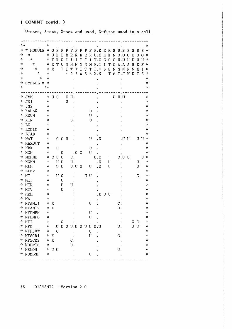
( COMINT contd. )


-------------------~~- -=-==- ............ --------- ------------;'f"#': * * ;'-( ~'( ~toDULE ~'( 0 p p p P.P p p p P.R R R s s.s s s s s "#'r

;'( ;'( ";'-( u E L R R.R R R R U.E E E N 0.0 0 0 0 0 ~'(

;'( ";"\ ;'-( T R 0 I I. I I I I T.G G G c u.u u u u u ~'(

;'-( ;': ;'; E T u N N.N N N N F. I I T 0 A.A A B E F ;'(

.. lr ;'( ~'( R T T T.T T T T 1.0 s s N N.N N N X I ;'-(

~'( ;'( ;'r 1 2.3 4 5 6 X.N T s I.J K D T s ;'-(

;'(

"" "k * ;'-( SYMBOL "i'r ~'( 'i'r

;" ';'(";'( "i'(

----------------------___ .... _____

--------- -----------;'-: JMM -;'-( u c u u. u u.u 'l'r

;'-( JN1 * u ;'-:

""k JM2 i" ..,.,

;'-( KAUSW ';'( u ;'-:

~'( KDUM "'"'

u """'

* KTR ;~ u. u ~'(

;': LC ;'-( ;'-(

;'r LCDIM 'i'r "i'r

"i'r LTAB ;'-( ~'(

"" MAT ";'-( c c u u .u .u u u u ;'-(

.. k MAXOUT ;'-( ;':

i'r ~1BK ;'r u u -;':

'i'( ~1CM ;': c .c c u ;':

'i'\ NCMML ;': c c c c. c.c c.u u u ;':

i'r HCMN ""/( u u u. .u u u t':

;'t NLM i': u u u.u u u .u u u ··}(

'" HLM2 'i': ;':

"'k MT "'k u c u u c ··/:

;'r HTJ -/: u ;':

;': NTR ;': u u. '"l:

;': MTV ;': u •;'(

'i': NZM "'/\ .X u u ~'(

;': NA ;'-( .. /, "'k NFANI 1 .. k X u c. "'l:

""k NFANI2 ;': X c. 'i'(

;': NFDMPN ~k u ;':

;'r NFDMPO ;': u ;':

;': NFI i': c c c i'(

"'k NFO ~'( u u u u.u u u u u.u u. u u 'i'(

;': NFPERT ""k c u "'k 'i'( NFSCR1 ;': X u c. ;'-(

.. k NFSCR2 ;" X c. .,, ~'( NOPNTS '"k u. ·k

;': NRMOM 'i'( u u u. •k

";'( NUMDMP ;': u ;':

---------------------- --------- --------- -----------. . .


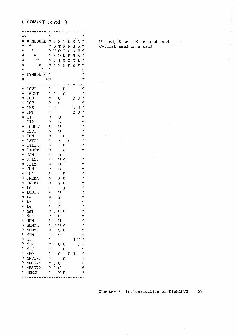
( COMINT contd. )

;'r

•'r •'r MODULE •'r S S T U X X * * * * 0 T R N S S * * * * U 0 I C C H * * * * S D N H H E * * * * C I E C C L * * * * A S R K K P *

..,., ICVT ;'\ u 'i'(

i': IGCNT ;'r c c "'' ...,., IGM ;': u u u ;'\

"" IGP i': u ..,.,

;'r IHS ;'( u u u ;':

•k IHT 'i': u u 'i'(

~/r II1 ;'r u ...,.,

;'( II2 'i': u "'r ·;'( I QUELL * u ;'(

t'\ ISCT ,., u ;'r

'"k ISN "k u 'i'(

;'r ISTOP ;'( X s ..,.,

;'\ I TL IM .. k u i':

;'\ ITOUT ... c ;':

... JJMM i': u ·#

i': JLIM2 i'r u c l'(

;': J1IM i': u "/\

;'r JMM 'i'r u ;':

;'r JM1 ;'( u ..,.,

'i'l JREBA "'k s u i': ';'\ JREBE i': s u ;'r ..,., 1C 'i'r X ;':

;'( 1CDIM i': u ;'r

'"k 14 ;'r s ;'r

"'k 15 ... s i':

t'r 16 ..,., s ;': ...,., MAT i'r u u u ... '"k MBK "k u ... ;': MCM i': u i':

'"k MCMM1 ;': u u c i':

;': MCMM ·# u u ;':

'i'( MLM 'f'( u ;'(

t'r MT i'r u u -;':

... MTR ..,., u u u ;'r

'i'( MTV i'l u t'r

•k NFO ;'( c u u '"k ;'( NFPERT ;'( c ;':

'i'( NFSCR1 i': c u .. k

'i': NFSCR2 ;'( c u i'r

·k NRMOM o.;'-( X u ;':



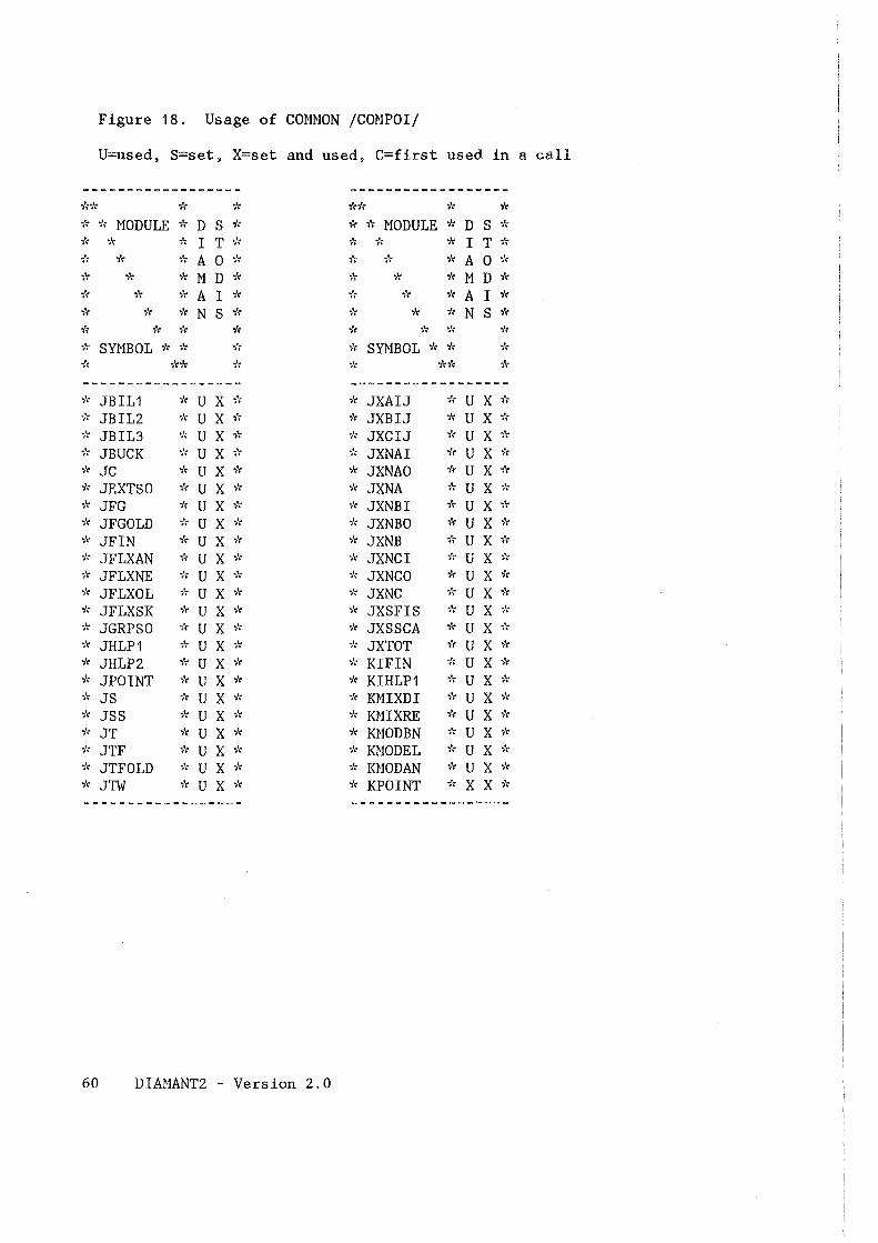
Figure 18. Usage of COHMON /COMPOI/


-------=====------ -------------------;'(";'( ";~ * ~'(* ~'( ~'(

";~ -;': MODULE -;'( D s "i'( 'i'c .,~ MODULE ~'( D s ~'(

~·r ~'( "i't I T -1: ";~ ~'( ,'( I T ";~

";'( ;'r "'i'r A 0 "i'r ~ .. .,., -;'( A 0 ..,.,

";"\ 'i'r 'i'r M D "i'r "i'r "i'r ";'( M D ~'(

,., "i'r ~'r A I ";'\ ';'( "i'r ..," A I "i'r ..,., "i'r ~'( N s ~·r ·,'( "i'r ~'r N s ~'(

"i'r ~'( "i'r -;'( ';'( "i'r .,., "i'f

~'r SYMBOL ~'r ~'r ·l'r ;': SYMBOL .,., ~'r , .. --:~ -;'r* 'i'r ..,., "'"~'( ~'r

------------------ ------------------;': JBIL1 ...,., u X 'i'r ;'( JXAIJ "i'r u X i'r "';'( JBIL2 ..,., u X ;'r ';'( JXBIJ ~'r u X •;'(

'"k JBIL3 ';'( u X 'i'r ~'r JXCIJ "'k u X ~ .. 'i'( JBUCK f'( u X ~'r ..,., JXNAI ..,., u X * i'r JC ';'( u X '"k ~'r JXNAO ~'r u X .,., ;'r JEXTSO ~'r u X ;'-( i'r JXNA 'i'r u X "i'r

'i'r JFG ;'r u X ~'-( ..,., JXNBI 'i'r u X 'i'r

'i'r JFGOLD .,., u X ·k .,., JXNBO ;'-( u X "k ";'( JFIN i'r u X ;'-( •-/: JXNB 'i'r u X .,., ··/: JFLXAN 'i'r u X .. ", ;'r JXNCI ..,., u X ;'r

"i'( JFLXNE 'i'r u X "i'r ;'r JXNCO 'i'r u X ..,., ..,., JFLXOL ;'r u X ;'-( ;'r JXNC 'i'r u X "'k

;'r JFLXSK "k u X ·k i'( JXSFIS ;'r u X ''k

'i'r JGRPSO ..,., u X ,., ..,., JXSSCA 'i'r u X ;'r ..,., JHLP1 "'k u X ~'-( .. /( JXTOT ;'-( u X ;'-(

~'r JHLP2 "i'r u X ";'( ··k KIF IN i'r u X "'k ·;'( JPOINT ...,., u X ... .. k KIHLP1 ";'( u X ";'(

-1: JS .,., u X * ;'r KMIXDI ··}( u X ~'r

-;'r JSS 'i'r u X ·-/( 'i'r KHIXRE 'i'r u X ;'r ..,., JT ;': u X "i'r ~'r KHODBN ·k u X ;'r

·k JTF i'r u X ~'r ..,., KHODEL ;'( u X 'i'r ..,., JTFOLD ;'r u X 'i'( •k KHODAN 'i'r u X "i'r .,., JThT 'i'r u X ;'r ";'\ KPOINT .,., X X i'\

=----------------- ------------------


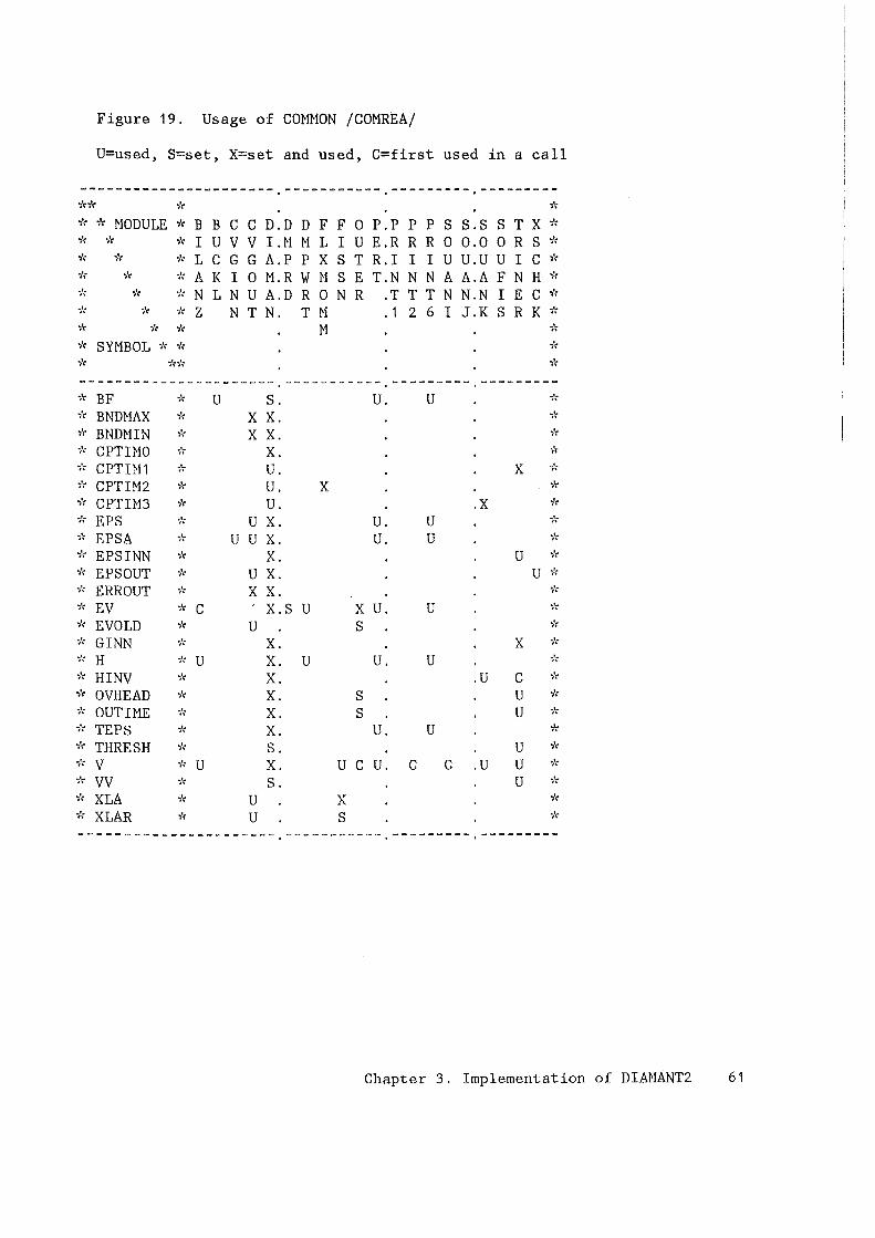
Figure 19. Usage of GONNON /CONREA/


---------------------- ----------- --------- ---------"';~';'; ..,., , .. ;': ..,, NODULE -/( B B c c D.D D F F 0 P.P p p s s.s s T X "#':

"'/( ;': i'( I u V V I. ~I M L I u E.R R R 0 0.0 0 R s "';':

;': ;'( i~ L c G G A.P p X s T R. I I I u u.u u I c "'k

•k ...,., , .. A K I 0 M.R w H s E T.N N N A A.A F N H ;'(

"'k ;': -1: N L N u A.D R 0 N R .T T T N N.N I E c -;':

;': ;': ;': z N T N. T H . 1 2 6 I J.K s R K , .. ;'( i': "k M ~~

";'\ SYMBOL , .. i': ·k

;': ;"r;': ;"(

---------------------- ----------- --------- ---------;': BF i': u s. u. u •k

i'( BNDMAX ;': X X. '"/(

·;'( BNDMIN "'k X X. 'i':

;': CPTH10 'i': X. ..,t,

t': CPTH11 'i'f u. X ;':

;\" CPTU12 ·k u. X ;':

;': CPTIM3 'i': u. .X .. k

;': EPS ;': u X. u. u "i':

i'( EPSA ;'( u u X. u. u ..,.,

.. k EPSINN i'\ X. u .. k

;': EPSOUT ..,., u X. u "'k

"'k ERROUT i'( X X. ..,.,

"'k EV ;': c x.s u X u. u ;'(

;': EVOLD ...,., u s ;':

;': GINN "k X. X •k

"'k H "'k u X. u u. u ·k

o.;'( HINV ;': X. .u c '"k ...,,, OVHEAD •/\ X. s u ;':

.. k OUT IME ;': X. s u ·k ..,., TEPS i': X. u. u * ";'( THRESH "'k s. u "t'(

"'k V ;': u X. u c u. c c .u u 'i':

i': vv ;': s . u ";'(

.. k XLA ;': u X ;'(

;': XLAR ';'\ u s ;':

----------------------.-----------.---------.---------


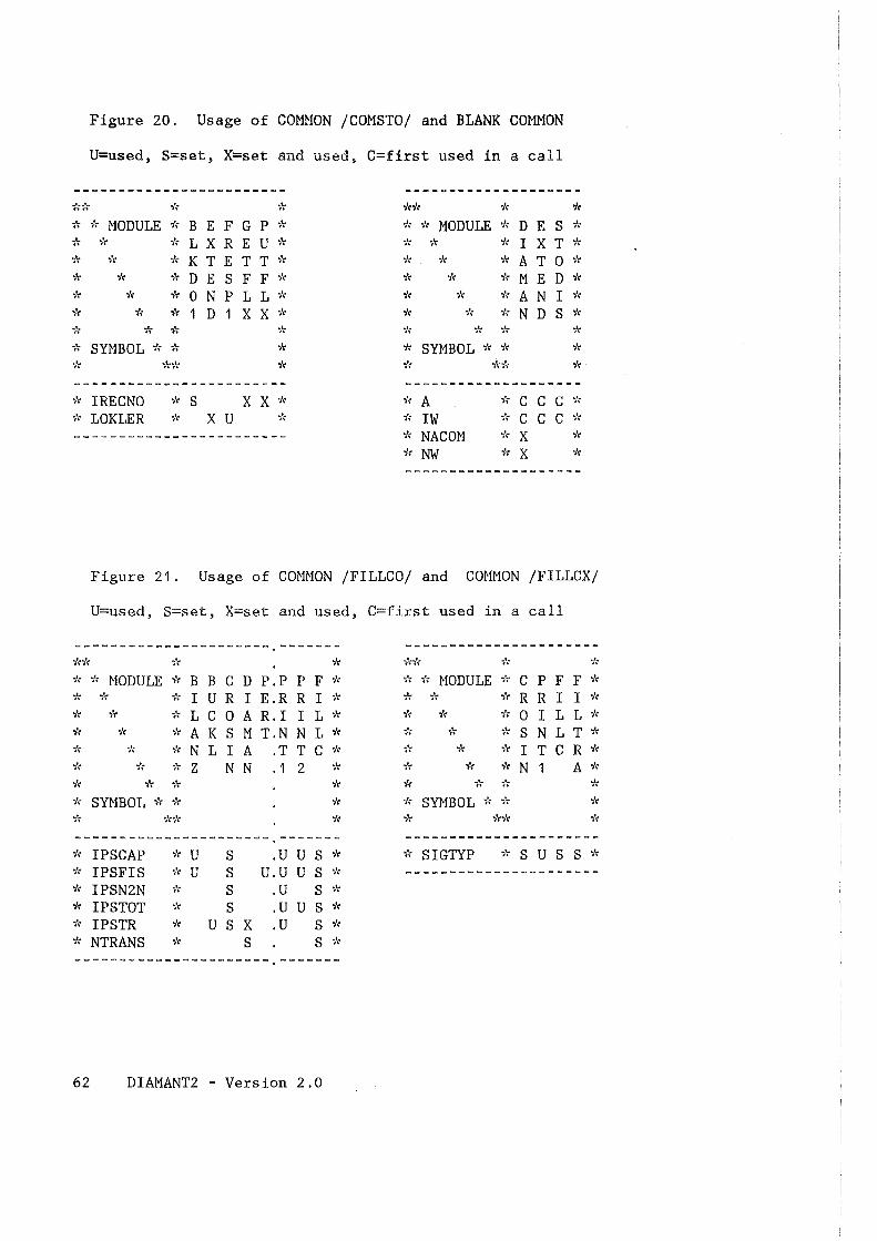
Figure 20. Usage of COMMON /COMSTO/ and BLANK COMNON


i~i't "'J': -.,'( ';'-(";'( ~·~ -~~

';'( ;'r MODULE ;'( B E F G p i': '?'r ";'( MODULE ..,., D E s ..,.,

~'r ..,., ;'r L X R E u i~ i't ;'r ~'r I X T i'-:

i'r i'r ;'( K T E T T ..,,, 'i'( ;'r i'-: A T 0 'i'\

;'( ..,~ 'i't D E s F F ";"( ;'c 'i'( ··k M E D ;'-(

;'r ;'r ;'r 0 N p L L ,., ;'( ;'r ·k A N I ..,.,

;'r 'i'\ i'-: 1 D 1 X X .,·~ 'i't ;'( ;'r N D s ;'(

'i'\ ;'r i't i': i': i'-: i': ;'(

i't SYMBOL 'i'( i't i'r ~'r SYMBOL i't ;'r ;'(

.,., *;" ;'-( •k .,~~" ;'(

--------------------.,·~ IRECNO .,·~ LOKLER

i't .,.,

A ;'(

IW ~k

c c c i't

c c c ..,,_

.,., NACOM "'k X .. k

'{~ NW i'r X ;'r

Figure 21. Usage of COMMON /FILLCO/ and COMMON /FILLCX/


----------------------* * MODULE * B B C D P.P P F * * * * I U R I E.R R I * * * * L C 0 A R.I I L * * * * A K S M T.N N L * * * * N L I A .T T C * * * * Z N N .1 2 *

---------------------- .... ------·k IPSCAP ·k u s .u u s .. k

i': IPSFIS i': u s u.u u s .,,, i': IPSN2N .,,, s .u s i'-:

* IPSTOT ..,., s .u u s ;'-(

~'r IPSTR i': u s X .u s i':

~ .. NTRANS i't s s ·;'(

---------------------- -------


t't•k i't .. k

i': ;'-( MODULE ;'( c p F F i':

* i'-: ;'( R R I I "'l\

i't ;'-( i't 0 I L L ;'r

-k i't i'r s N L T i't

i''( ;'t ;''( I T c R i':

i't ;'r ;': N 1 A .,., i't ;': .. k .. ;'( ;'r SYMBOL 'i'\ i't i't .,., "'}\i't ~·~

.,., SI GTYP ~r S U S S .,.,

3.3.3 Data Files Used

All data files in DIAMANT2 are accessed by calling entries of subroutine

READKO /9/. In this way, all binary I/0 operations are centralized and can

easily be modified (see "KAPROS Implementation" on page 69).

The data files NFSCR1 and NFSCR2 are used for intermediate binary storage

of calculated scalar fluxes. NFSCR1 is an input variable (see input card

K4) and NFSCR2 is equal to NFSCR1+1. They are only used if the main memory

available is not sufficient to store scalar fluxes for all energy groups.

Associated operating system control cards should always be supplied for

reasons of safety (example given for IBN environment):

//G.FT"NFSCR1"F001 DD DISP=(NEW,DELETE),DCB=(RECFH=VBS,BLKSIZE= ..... )

/ /G. FT"NFSCR2 "F001 DD DISP=(NEW, DELETE), DCB=(RECH1=VBS, BLKSIZE= ..... )

NFANI1 and NFANI2 are binary working data files which are only required for

the anisotropy option and contain the calculated flux moments (operating

system control cards analogaus to those before). NFANI1 is an inputvariable

(see input card K4) and NFANI2 is equal to NFANI1+1. These two files are

used only if the space reserved in GONNON block /CONNON/ (defined by a

PARANETER statement) is not sufficient to hold all flux moments. See also

"Tuning Binary Input/Ouput" on page 89.

Data file NFDHPN contains incoming angular fluxes, scalar fluxes, neutron

sources, and some auxiliary values in binary form at the end of each outer

iteration. NFDHPO contains a flux guess in the same format used in NFDHPN.

Both data files are only used if the input values of NFDHPN and/or NFDHPO

on input card K2 are greater than 0. If NFDHPN = NFDHPO, the flux guess from

NFDNPO is read first and the newly calculated flux is stored (after each

outer iteration) behind the last flux guess on NFm1PO. The structure of this

data file is described in "Structure of Restart Dump Files" on page 65.

Data file NFPERT serves as a binary interface file for the perturbation

module TPTRIA. The structure of this file is described in "Structure of

Interface File for Perturbation Hodule" on page 66.


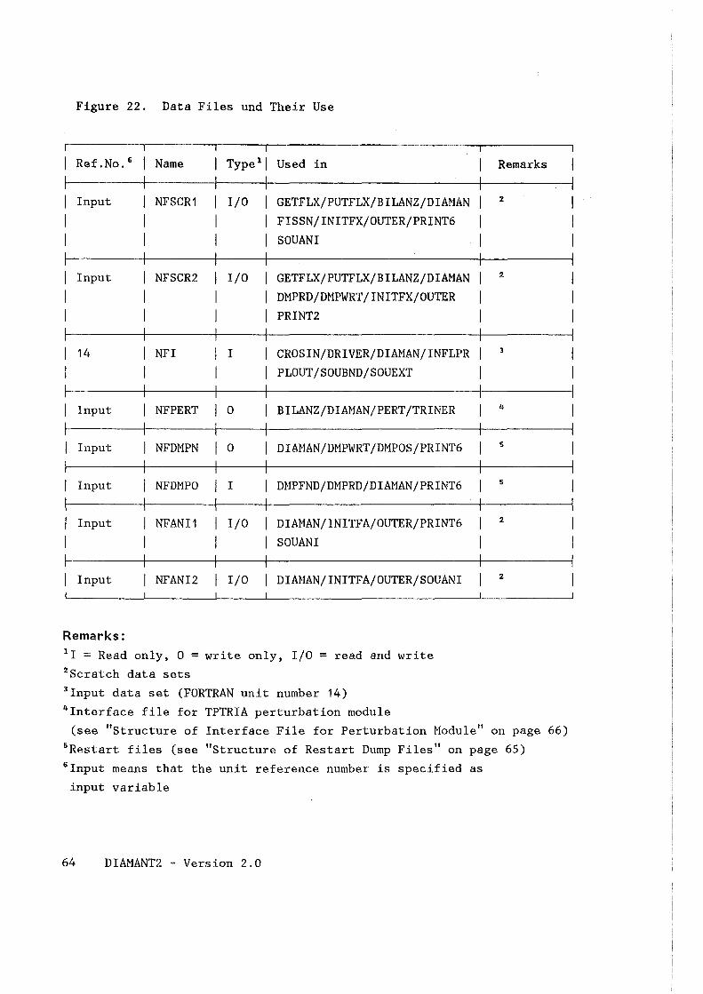
Figure 22. Data Files und Their Use

Ref.No. 6 Name Type 1 j Used in

Input NFSCR1 I/0 GETFLX/PUTFLX/BILANZ/DIAHAN FISSN/INITFX/OUTER/PRINT6 SOU ANI

Input NFSCR2 I/0 GETFLX/PUTFLX/BILANZ/DIAHAN DHPRD/DHPWRT/INITFX/OUTER PRINT2

14 NFI I CROSIN/DRIVER/DIAHAN/INFLPR PLOUT/SOUBND/SOUEXT

Input NFPERT I o BILANZ/DIAHAN/PERT/TRINER

Input NFDHPN 0 DIAHAN/DHPWRT/DHPOS/PRINT6

Input NFDHPO I DHPFND/DHPRD/DIAHAN/PRINT6

Input NFANI1 I/0 DIAHAN/INITFA/OUTER/PRINT6 SOU ANI

Input NFANI2 I/0 DIAHAN/INITFA/OUTER/SOUANI

Remarks: 1 1 = Read only, 0 = write only, I/0 = read and write 2 Scratch data sets 3 Input data set (FORTRAN unit nurober 14) 4 Interface file for TPTRIA perturbation module

Remarks

2

2

3

4

5

5

2

2

(see "Structure of Interface File for Perturbation Hodule" on page 66) 5 Restart files (see "Structure of Restart Dump Files" on page 65) 6 Input means that the unit reference nurober is specified as input variable


3.3.4 Storage Optimization Levels

Depending on input variables and on the available computer main memory,

DIAMANT2 has two levels of operation:

in the first one, Optimization 1, the whole problern can be solved core

contained (which is preferable from the standpoint of computing time)

in the second one, Optimization 2, the fluxes of one group are in-core,

the other ones being stored on disks NFSCR1 and NFSCR2. For reasons of

safety, these two files should be defined in any run.

The length of the working array needed depends on chosen input options (see

"How to Estimate Storage Needs" on page 81). Its estimation is a very tedious

process. It is recommended to let do this the input check module (see "Input

Test Module DIAPRD" on page 78). If possible one should avoid to run the

code in optimization level 2 because of performance degradation. In order

to avoid such a degradation, one should try the following: for the KAPROS

version one simply provides more main memory space by increasing the REGION

parameter on the JOB card; for the stand-alone version one has to increase

the values NAMAX and NWMAX in the PARMIETER statement (which normally means

an increase in the requested job REGION too) and to re-compile the code.

3.4 INTERFACES TO OTHER PROGRAMS

3.4.1 Structure of Restart Dump Files

These dump-files are used to provide a restart capability to DIANANT2 as well

as to provide flux and source guesses. They are read/written in subrautirres

DHPRD/DMPWRT. The logical structure is subdivided into variable length

records. For a definition of the dimensioning variables see Figure 10 on

page 46.

Record 1 Label record (see Figure 23 on page 67), 8 integer numbers and

2 reals


Next 3*1GM Records

JMM*JLIM2 real numbers written out separately for each possi

ble orientation of the system boundary and for each energy

group.

next IGM records

HCMML real numbers representing the (centered) scalar flux

values for each energy group

next record HCMML real numbers representing the fission source density

last record IGM+1 real numbers for the groupwise volume integrated fission

source (entry IGM+1 contains the group sum)

All records are readjwritten in binary form, i.e., without format control.

Dumps from several different calculations could be contained on a single

dump-file. The program identifies them by their relative position on that

file. The end of the dump-file is marked by a record containing 10 negative

integer numbers.

If a certain restart dump is requested to be used, the code checks whether

the structure of that particular dump fits to the current input data. If not

so, DIAMANT2 reads the whole restart file and selects the first dump having

suitable dimensions. If this procedure fails too, DIAMANT2 uses a code

generated (flat) source guess. Warning messages are printed in any case.

3 .4. 2 Structure of Interface File for Perturbation Module

This interface file is presently used by the perturbation module TPTRIA

/3/. It contains - besides some control information - the angular fluxes

calculated during the last outer iteration for each group. Again this is a

binary file. For a definition of the dimensioning variables see Figure 10

on page 46.

Record 1 input card K1, 60 characters label

Record 2 from input card K2 variables

ID, ITH, ISN, IGM, IEVT, MLM, MCMM(=Z~'rMCM), MT, HAT, INBO


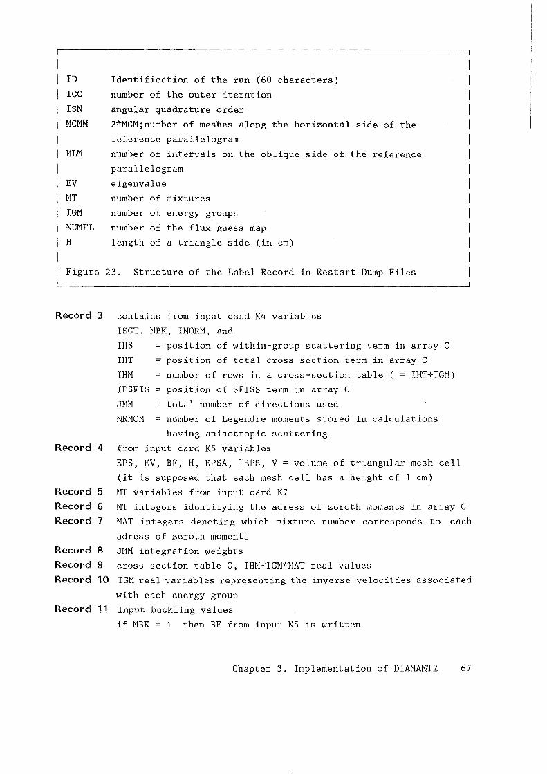
ID

ICC

ISN

MCMM

MLM

Identification of the run (60 characters)

nurober of the outer iteration

angular quadrature order

2~'>'MCM;number of meshes along the horizontal side of the

reference parallelegram

nurober of intervals on the oblique side of the reference

parallelegram

EV eigenvalue

MT nurober of mixtures

IGM

NUMFL

H

nurober of energy groups

number of the flux guess map

length of a triangle side (in cm)

Figure 23. Structure of the Label Record in Restart Dump Files

Record 3 contains from input card K4 variables

ISCT, NBK, INORM, and

IHS = position of within-group scattering term in array C

IHT = position of total cross section term in array C

rm1 = number of rows in a cross-section table ( = IHT+IGH)

IPSFIS = position of SFISS term in array C

JMM = total number of directions used

NRMOM = nurober of Legendre moments stored in calculations

having anisotropic scattering

Record 4 from input card KS variables

EPS, EV, BF, H, EPSA, TEPS, V = volume of triangular mesh

(it is supposed that each mesh cell has a height of 1 cm)

Record 5 MT variables from input card K7

cell

Record 6 MT integers identifying the adress of zeroth moments in array C

Record 7 HAT integers denoting which mixture number corresponds to each

adress of zeroth moments

Record 8 JMM integration weights

Record 9 cross section table C, IHM~·~rGM•'<'MAT real values

Record 10 IGM real variables representing the inverse velocities associated

with each energy group

Record 11 Input buckling values

if MBK = 1 then BF from input KS is written


if HBK = 2 then input K14A is written (IGM values)

if HBK = 3 then input K14B is written (IGH~'rHT values)

Record 12 HCHHL integer values containing the mixture numbers associated

with each spatial cell, starting from upper left triangle to lower

right triangle and row-wise from left to right.

Record 13 JMH integer values identifying the sequence in which discrete

directions are worked on

Record 14 (written only in anisotropic cases)

NRHOH*JHM real values containing the spherical harmonics values

for each direction.

Records 15 - 17 are repeated for each energy group and for each "real"

direction (out of the JHH discrete directions defined, only JHH-ISN are used,

the remaining ISN being dummy).

Record 15 one integer number identifying the actual group

Record 16 one integer number identifying the order number of the actual

direction

Record 17 HCMHL real numbers containing the (centered) angular fluxes for

that group and that direction in same order as in Record 12

Records 18- 22 may appear several times (see remark 4 below).

Record 18 Number of groups (same as variable IGM)

Record 19 Number of records 21,22 (variable IND)

Record 20 Criticality factor

Records 21,22 are repeated IND-times (see remarks 1, 2, 3 below)

Record 21 number of table given as record 22

Record 22 total fluxes (IGH real values)

Remarks

1. Variable IND is equal to 1 for the first set of records 18 to 22. The

groupwise volume integrated fluxes then correspond to those of global

balances. These total fluxes are always written.


2. Variable IND is equal to MT if KAUSW is equal to 10 or 11 (KAUSW is an

input variable on input card K4 and triggers the calculation of bal

ances). In this case the groupwise total fluxes are written separately

for each mixture number ( i. e. , MT tim es) .

3. Variable IND is equal to the number of different regions in the layout

if KAUSW = 1 or 11. In this case the total fluxes are written separately

for each region.

4. Depending on the value of KAUSW, the set of records 18 to 22 is written

once (KAUS\v = 0) or twice (KAUSW = 1 or 1 0) or three times (KAUSW = 11).

5. If the interface file has been generated by an adjoint calculation one

should be aware of the different interpretation of group order and

angular orientation (see "Adjoint Calculations" on page 23). With

exception of the cross section matrix C, all values are given in reverse ..... group ordering; angular fluxes of direction Q have to be interpreted as

be longing to 4.

3.5 KAPROS IMPLEMENTATION

Within KAPROS it is possible to use datablocks instead of disk data sets.

Using the READKO /9/ package one has the possibility to determine at program

running time whether a data file should be realized as a KAPROS data block

or as a (module-owned, external) tape or disk data file.

Figure 24 gives a description of the (proposed) content of

DBN = INITPREADf:>DIAHAN which must be provided in the KAPROS lifeline when

calling DIAHANT2. It is read by READKO and controls the realization of the

individual data files. Basically, all options listed in /9/ can be selected,

although it is advised not to deviate from the recommended values.

If NFDHPN = NFDHPO, unit NFDHPN has the same data block name as NFDHPO; only

the space requirement for the actual case under consideration is indicated

under file length for NFDHPN in Figure 24.


Within the KAPROS system, the subroutine package FILLC allows DIAMANT2 to

read nuclear cross-sections from a binary file having the so-called SIGMN

/11/ structure. This option can ease input preparation quite a lot since

cross section data has not to be entered by hand.

Within the KAPROS system, NACMAX (length of the real working array) as well

as NWMAX (length of the integer working array) are equal to one. After

having determined the amount of storage needed (depending on input values),

DIAMANT2 calls a special KAPROS rout ine, KSPUTP, to dynamically extend

arrays. The real storage is provided in a KAPROS data block DBN=DIAM215REAL~'<'4

with a corresponding pointer JPOINT (relative to A(1)), the integer storage

is located in DBN=DIAM215INTEGER*4 with a corresponding pointer KPOINT (rel

ative to IW(1)). The distribution of the working arrays is the same as in

the stand-alone version.

DIM1ANT2 is stored in the KAPROS module library with name DIANEU and is

invoked by either the command

or the call

CALL KSEXEC('DIANEUI515', .... ).

See /4/ for further details. Note that at least the input data blocks

DBN=DIAMANT215EINGABE and DBN=INITISREAD!SDIAMAN, both with index 1 have to be

known at the module level of DIAMANT2.


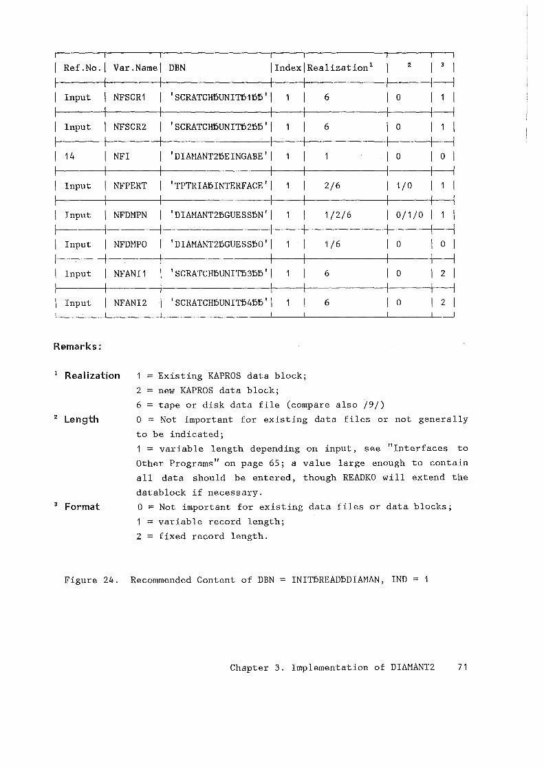
Ref .No.l Var.Namel DBN 1Index1Realization1 2 I 3

Input NFSCR1 1 SCRATCHöUNI~1Öo 1 1 6 0

Input NFSCR2 1 SCRATCHöUNI~2Öo 1 1 6 0

14 NFI 1DIAHANT2öEINGABE I I 0 0

Input NFPERT 1TPTRIAöiNTERFACE 1 I 2/6 1/0

Input NFDMPN I DIMIANT2bGUESSöN I I 1/2/6 0/1/0

Input NFDHPO I DIAHANT2öGUESSöO I I 1/6 0 0

Input NFANI1 1 SCRATCHöUNI~3ÖD 1 I 6 0 2

Input NFANI2 1 SCRATCHöUNI~4ÖD 1 I 6 0 2

Remarks:

1 Realization = Existing KAPROS data block;

2 = new KAPROS data block;

2 Length

3 Format

6 = tape or disk data file (compare also /9/)

0 = Not important for existing data files or not generally

to be indicated;

1 = variable length depending on input, see "Interfaces to

Other Programs" on page 65; a value large enough to contain

all data should be entered, though READKO will extend the

datablock if necessary.

0 =Not important for existing data files or data blocks;

= variable record length;

2 = fixed record length.

Figure 24. Recommended Content of DBN = INI~READöDIAMAN, IND =


3.6 USE AS STAND-ALONE PROGRAM

3.6. 1 General Remarks

The DIAMANT2 code is designed such that it is very easy to produce a version

which runs without support by KAPROS (''stand-alone" version) as well as an

equivalent version running under control of KAPROS. The following diagram

illustrates schematically those portians of DIAMANT2 which are directly or

indirect ly dependent upon KAPROS and which differ in coding between the

KAPROS and the stand-alone version.

Most of the KAPROS dependent subroutines serve as aids in input preparation

(FILLC, READKO) or add dynamic features (EXTEND) to DIANANT2. As will be

illustrated in the following, the KAPROS dependent portians are very easily

replaced by stand-alone simulations.

3.6.2 Subroutine EXTEND

Used to distribute working arrays among code arrays.

KAPROS-version Dynamically allocates pointer data blocks to hold

working arrays

Stand-alone version Allocates in blank COMMON/ I the amount of storage

place needed according to input specifications


-----------------

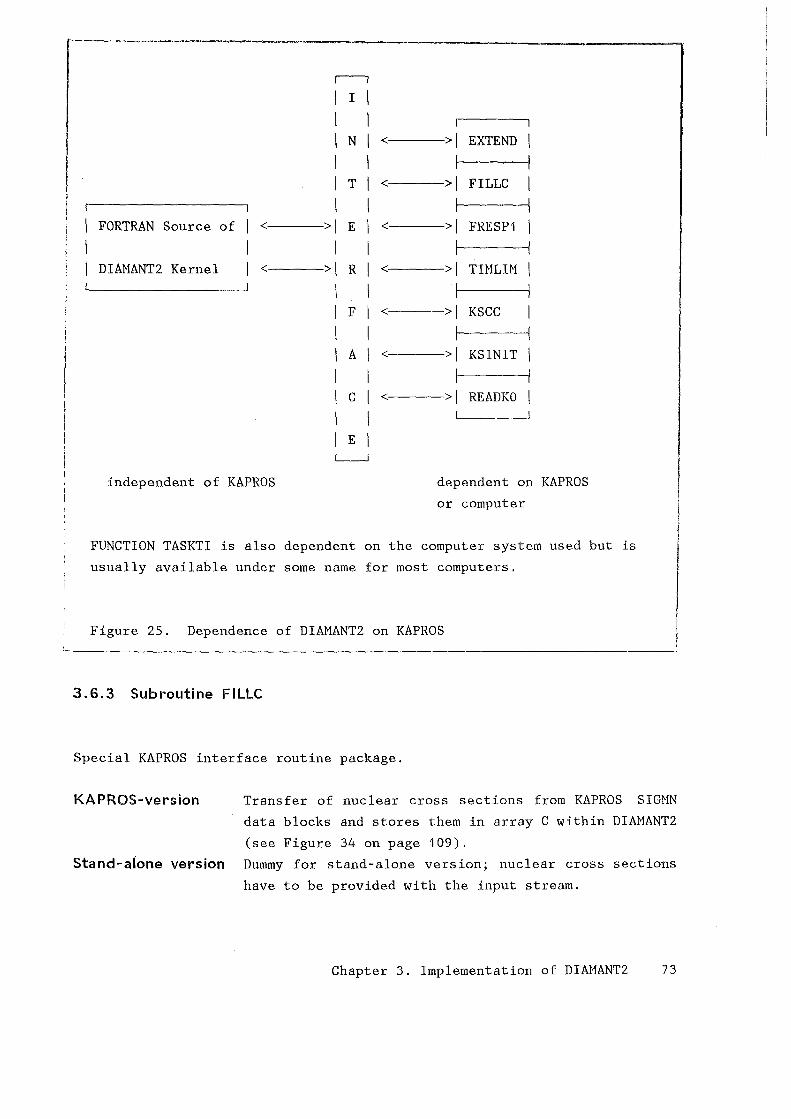
r--1

I I I

N I < >I EXTEND

I I T I < >I FILLC

I I FORTRAN Source of I < >I E I < >I FRESP1

I I I DIAMANT2 Kernel I < >I R I < >I TU1LIM

... J I I I F I < >I KSCC

I I I A I < >I KSINIT

I I I c I < >I READKO

I I I E I L___j

independent of KAPROS dependent on KAPROS

or computer

FUNCTION TASKTI is also dependent on the computer system used but is

usually available under some name for most computers.

Figure 25. Dependence of DIAMANT2 on KAPROS

·--------------------------------------------------------------------------

3.6.3 Subroutine FILLC

Special KAPROS interface routine package.

KAPROS-version Transfer of nuclear cross sections from KAPROS SIGMN

data blocks and stores them in array C within DIAMANT2

(see Figure 34 on page 109).

Stand-alone version Dummy for stand-alone version; nuclear cross sections

have to be provided with the input stream.


3.6.4 Subroutine FRESP1

Used for informative output only.

KAPROS-version Amount of free storage places in the allocated computer

main memory

Stand-alone version Gives the amount of working storage still not allocated

in working arrays (defined by PARMiETER' s NAGMAX and

N\VMAX).

3.6.5 Function TASKTI

Returns the GPU-time (in seconds) used already for the task up to the moment

of calling TASKTI. Used to calculate timing statistics.

KAPROS-version Uses a compiler service function

Stand-alone version Uses a compiler service function (such a function is

usually provided along with a compiler (like SEGOND for

GRAY and GYBER, GLOGKM for SIEMENS; or one has to pro

gram some simulation like JTIME for IBM in IBM ASSEN

BLER).

3.6.6 Function TIMLIM

Returns the remaining GPU-time (in seconds) for the job. Used to prevent a

task breakdown due to exhaustion of GPU resources and to allow a controlled

termination.

KAPROS-version Uses an ASSEMBLER function JTIME out of the KAPROS

kernel system

Stand-alone version A machine dependent routine has to be used (TREMA! for

GRAY, JTIME for SIEMENS and IBM, JTIME simulation for

GYBER). For IBM, SIEMENS, GRAY and GYBER running ver-


sions of TIMLIM are provided along with the source deck

of DIAMANT2.

3.6. 7 Subroutine KSCC

Used to respond to erroneous situations.

KAPROS-version Sets and re-sets error codes; part of the KAPROS kernel

Stand-alone version executes a STOP statement in case of any error

3.6.8 Subroutine KSINIT

Special KAPROS interface routine.

KAPROS-v~rsion Initialization of the KAPROS kernel

Stand-alone version Initializes unit numbers for standard read/print files

3.6.9 Subroutine READKO

This is an interface package for binary input/output operation. It is fairly

simple for the stand-alone-version and very elaborated for the KAPROS ver

sion. For details see /9/.

See "Tuning Binary Input/Ouput" on page 89 for details how one may improve

performance of I/0 operations on computers having a very large main memory.


CHAPTER 4. TEST EXAMPLES AND USER INFORMATION

4.1 TEST CALCULATIONS CARRIED OUT

An elaborated series of test calculations has been carried out with DIAHANT2.

These will be documented separately /14/. Herewe will give only an overview

about the test cases and the main findings from those calculations. The

following is a list of the major test cases executed:

..

..

..

k~ for infinite homogeneaus regions;

Irrdependance of results on the position of the model in the reference

frame;

adjoint calculations;

anisotropy option;

buckling options;

external source calculations;

usage of restart dumps;

runs in different storage optimization levels.

In addition to these, a number of parameter variations have been clone in

order to estimate the influence of the input variables EPS, EPSA, IIH, IIL

and ISN on numerical results and computing time. Derived recommendations may

be föund in "Experience From the Test Calculations" on page 78. Input for

most of the test examples is distributed along with the source code.

Chapter 4. Test Examples and User Information 77

4.2 INPUT TEST MODULE DIAPRO

A separate module DIAPRO is available for input testing again in a stand

alone Version and as KAPROS module. DIAPRO reports the input in clear text

and produces a sketch of the mixture distribution. The application of this

check module appears to be particularly useful for testing newly produced

inputs because it uses almost no computer resources.

In addition to input testing, it also calculates how many words of main

memory are required for the individual working fields. DIAPRO provides

information concerning these values as well as working data files which may

be necessary (see also "Storage Optimization Levels" on page 65).

DIAPRO is stored in the KAPROS module library and is invoked by specifying

~'<'KSIOX DBN= ..... , PMN=DIAPRD

See /4/ for further details. Note that at least the input data blocks

DBN=DIAMANT2~EINGABE and DBN=INI~READöDIAHAN, both with index 1 have to be

known at the module level of DIAPRD.

4.3 EXPERIENCE FROM THE TEST CALCULATIONS

4.3. 1 How to Choose the Quadrature Set

For problems dominated by the diffusion of neutron through optically thick

regions, a PN approximation may be expected to yield superior results to the

DPN approximation. In contrast, the DPN quadrature may be preferable for

problems dominated by the presence of boundaries, particularly vacuum boun

daries. A more detailed discussion of these aspects may be found in /8/.

The differences between PN and EPN sets are usually small. For details how

the quadrature set is constructed see "Construction of SN-Constants" on page

8 and "Appendix A. DIAHANT2 Built-in Quadrature Constants" on page 119.


SN-orders rauging from 2 to 12 are built-in. One should bear in mind that

DIANANT2 for a given order ISN has SO% more directions compared to conven

tional 2d geometry SN-codes (because of the division of the unit sphere into

dodecants instead of the usual octants). In our test cases results did not

change very much beyond ISN=8.

4.3.2 How to Choose Iteration Control Parameters

There are basically five input values to control the iteration process. The

easiest one to choose is ICH, the maximum nurober of outer iterations. In

our tests we used values between SO and 100. Goropared to the old version

/1/, the new code needs more outer iterations but the total nurober of inner

iterations is not changed very much or is even lower. The value of ICH is

not very important because a threatening time limit break down of the task

will be prevented by the timing function TIHLIH.

The next two parameters, IIL and IIH, are the maximum nurober of inner iter

ations for the first outer iteration and the absolute maximum nurober not to

be exceeded in any outer iteration, respectively. IIL is increased from one

outer iteration to the next by 1 until IIH is reached. For an efficient

iteration, IIL should be small (something like 2 or S) and IIH large (some

thing like 20 or 30). When using a restart dump, IIL should be larger

(something like 10). This is especially important if one uses a dump to

start a calculation with anisotropic scattering.

The parameter EPSA is the precision wanted for scalar fluxes. How 11precision11

is defined and estimated is described in "Inner Convergence Tests and Con

vergence Acceleration11 on page 19. Since the actual precision threshold

during inner iterations is set to

EPSINN = HAX {HIN { EPSINN, 0.1*E t } ,ABS(EPSA) }, ou er which depends on the convergence E t achieved for sources, the nurober of ou er inner iterations does not depend very much on the value of EPSA during the

early phase of the iteration process. Values of EPSA in the range 1.0E-3

to 1 .OE-5 have been used in our tests.


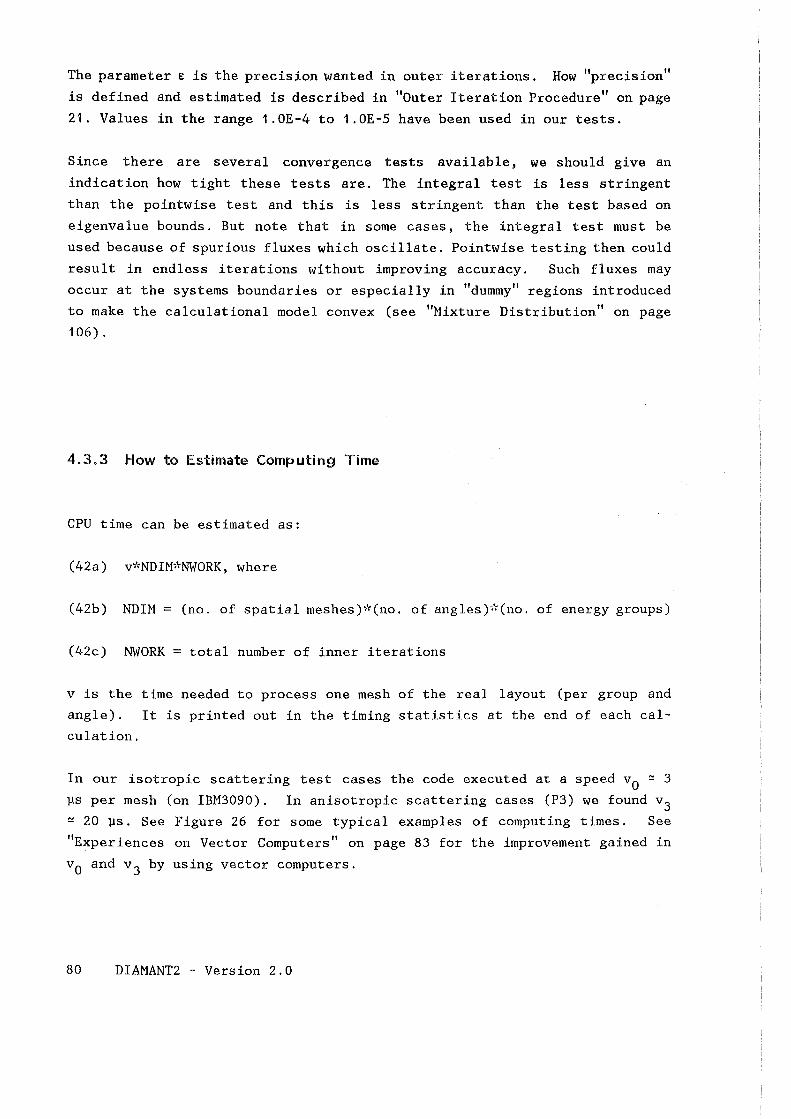
The parameter E is the precision wanted in outer iterations. How "precision"

is defined and estimated is described in "Outer Iteration Procedure" on page

21. Values in the range 1.0E-4 to 1.0E-5 have been used in our tests.

Since there are several convergence tests available, we should give an

indication how tight these tests are. The integral test is less stringent

than the pointwise test and this is less stringent than the test based on

eigenvalue bounds. But note that in some cases, the integral test must be

used because of spurious fluxes which oscillate. Pointwise testing then could

result in endless iterations without improving accuracy. Such fluxes may

occur at the systems boundaries or especially in "dummy" regions introduced

to make the calculational model convex (see "Hixture Distribution" on page

106).

4.3.3 How to Estimate Computing Time

CPU time can be estimated as:

(42a) v•'<'NDIM•'<'NWORK, where

(42b) NDIM = (no. of spatial meshes)*(no. of angles)*(no. of energy groups)

(42c) NWORK = total number of inner iterations

v is the time needed to process one mesh of the real layout (per group and

angle). It is printed out in the timing statistics at the end of each cal

culation.

In our isotropic scattering test cases the code executed at a speed v0 ~ 3

~s per mesh (on IBM3090). In anisotropic scattering cases (P3) we found v3 ~ 20 ~s. See Figure 26 for some typical examples of computing times. See

"Exper iences on Vector Computers" on page 83 for the improvement gained in

v0 and v 3 by using vector computers.


I I I I I I I I I I I I I I I I I I I I I

ISCT

0

0

0

3

3

3

Grid size I no. of meshes

17x171 289

38x38l 1156

57x5712601

17x17 I 289

38x38l1156

57x57l2601

Storage

kBytes

568

736

984

776

1308

2164

CPU timel Speed

sec

23

78

175

66

261

585

llSeC

3.2

2.8

2.8

19.2

18.4

18.8

taver

msec

16. 1

55.1

122.4

99.4

384.3

880.3

ISCT = anisotropy order; taver = average time per inner iteration;

Storage= needed for working arrays.

All values given for 87890 computer; all

groups and S4 approximation; convergence

ces and fluxes based on pointwise tests.

examples use four energy

criteria are 1.0E-4 for sour-

I Figure 26. Examples for Storage, CPU Times and Execution Speed

4.3.4 How to Estimate Storage Needs

Ta a first order approximation the storage amount needed is:

(43) Storage = (Codelength) + (Grid Size)*(A + B*IGM) + C*IGM in words

where A = 11, B = 2 and C ::::: 6~'•JJMM and Grid Size is the number of meshes

of the reference parallelogram. Using the anisotropy option .these values

change to A = 11+2*NRMOM+JMM, C = 6*JJMM+JMM*NRMOM (B same as before). IGM

is the number of energy groups, JMM the number of discrete directions, JJMM

the number of intervals on one side of the reference parallelogram times JMM

and NRMOM the number of stored anisotropic moments. On IBM Codelength :o!

70000 words.


According to the authors' experience it is easiest to let the code estimate

its exact storage need for a particular case. One easily could start the

DIAMANT2 or DIAPRD (see "Input Test Module DIAPRD" on page 78) with a small

amount of CPU time and then analyse the output. On the first few pages there

is a complete information on storage needs. For reasons of efficiency, any

calculation should be run in storage optimization 1 (i.e. fully core-con

tained) as long as there is the possibility to get enough main memory from

the operating system. See Figure 26 on page 81 for some typical examples

of storage requirements and "Storage Optimization Levels" on page 65 for

recommendations.

4.3.5 Discretization Accuracy

In criticality calculations we observed a fairly good linear dependence of

keff on the (constant) mesh volume. This means that at least for this

parameter, DIAMANT2 is O(h 2) accurate.

On CYBER-205, the code executes in eight bytes mode. Camparisan of results

obtained from test calculations on CYBER-205 and IBM led us to the statement

that usually single precision is sufficient on IBM equipment (i.e. in four

bytes mode) to get reliable results of 4-5 digits in keff and integrated

quantities and 3-4 digits in fluxes.

4.3.6 The Role of Negative Flux Fix-Up

In the present version, negative flux fix-up is activated only after con

vergence of iterations. Usually only very few meshes need a fix-up and cor

respondingly only a few (1 to 5) additional iterations are needed for final

convergence. The nurober of meshes which suffered a fix-up step is printed

in the iteration monitor. If this nurober is large ceropared to the total

nurober of meshes, results will probably have a lower accuracy than mentioned

above. In these cases one may try to avoid negative fluxes by using a finer

spatial mesh grid and a higher SN order.


4.4 EXPERIENCES ON VECTOR COMPUTERS

DIAMANT2 has been successfully run on CYBER-205, GRAY, IBM-VF and

SIEMENS/FACOM VP vector computers. Only the most time consuming routines

(see "Function of the Different Subroutines" o~ page 41) have been compiled

with "autovectorization on". Note that DIAMANT2 is completely written in

FORTRAN77 (except for the timing functions). The timings giving in the fol

lowing refer to a common source deck. At a few places we have inserted com

piler directives to improve vectorization. In the case of the CYBER-205,

the autovectorizer FTN200 does not substantially vectorize the code. The

CYBER-205 entries "autovectorized11 given in the table have been obtained

using the VAST /16/ preprocessor. It is clear, that using special language

extensions on a vector computer could enhance the performance at the cost

of creating a less portable code.

In DIAMANT2, the vector length for the most time consuming loops is usually

the length of one line of meshes during space-angle mesh sweeps in inner

iterations. Moreover, the length of a line can be different from line to

line. At the top of the iteration monitor the code prints some information

on the vector lengths (minimum, maximum and average) encountered. There are

many loops having a length equal to the total nurober of spatial meshes, but

these do normally not contribute much to CPU time consumption.

We have run isotropic calculations with an average vector length of 12, 27

and 41. There we observed speed-ups in the range of 2 to 4 (see Figure 27

on page 84). The vectorization degree (defined as the ratio of total time

to vector time) has been measured on VP100 tobe 0.5 (for vector length 12)

and 0.8 (for vector length 41). Higher speed-up and higher vectorization

degree can be expected for larger cases or by hand-tuning of a couple of

loops in subroutine TRINER.

The ranking of vector computers in the above examples is CRAY-XMP : CYBER-205

: SIEMENS-VP : IBM-VF, reflecting both, hardware and compiler efficiency.

For cases using a Legendre expansion of the scattering kernel, vectorization

has a much more pronounced effect. Using that option necessitates to update


Computer! Vector I Speed Speed Speed Perfor-

type length 1 I psec 2 up3 up4 mance 5

CYBER6 12 5.516 I 3.096 1.8 0.9 0.47

27 4. 780 I 1. 732 2.8 1.3 0.48

205 41 4. 772 I 1. 300 3.7 1.7 0.47

CRAY 6 12 2.968 I 1 . 216 2.4 2.2 0.88

27 2.756 I 0.816 3.4 2.8 0.83

XMP 41 2.552 I 0.692 3.7 3.2 0.88

FACOM 6 12 2.616 I 1 . 912 1. 4 1.4

27 2.284 I 1. 008 2.3 2.3 1. 00

VP100 41 2.240 I 0.740 3.0 3.0

IBM 6 12 2.432 I 2.096 1. 2 1 . 2 1. 08

27 2. 116 I 1 .408 1.5 1. 6 1.08

VF 41 2.108 I 1. 328 1 . 6 1 . 7 1. 06

CYBER 7 12 6.292 I 3.068 2.1 1. 0 0.50

XMP 7 12 3.682 I 1.272 2.9 2.5 0.86

VP100 7 12 3.172 I 1. 963 1 . 6 1 . 6 1. 00

VF 7 12 2.964 I 1. 659 1. 8 1 . 9 1. 07

1The average length of lines is the dominating vector length in cases

using isotropic scattering. 2 Given in the form : scalar I autovectorized CPU time. 3 Speed-up given as ratio of scalar over autovectorized computing time. 4Speed-up given relative to the execution time on a SIENENS7890 5 Performance given as ratio of scalar execution time on SIEMENS7890 over

scalar execution time on vector computer. 6 Using 4 energy groups and an s4 approximation. 7Using 26 energy groups and an s6 approximation.

Figure 27. CPU Times for Some Vector Computers (Isotropie Scattering)


Camputeri Vector I Speed Speed Speed Perfor-

type length 1 1 11sec 2 up3 up4 mance 5

CYBER 6 578 34.23 I 5.308 6.4 2.4 0.38

2592 30.98 I 2.952 10.5 3.9 0.37

205 6050 30. 10 I 2.340 12.9 5. 1 0.40

CRAY 6 578 18.23 I 2.336 7.8 5.5 0.71

2592 16.71 I 1 . 712 9.8 6.7 0.69

XHP 6050 16.58 I 1.540 10.8 7.8 0.72

FACOM 6 578 12.92 I 2. 972 4.4 4.4

2592 11 . 50 I 1.768 6.5 6.5 1. 00

VP100 6050 11 . 98 I 1. 456 8.2 8.2

IBM 6 578 11 . 35 I 6.716 1 . 7 1 . 9 1 . 14

2592 10.30 I 5.388 1 . 9 2. 1 1 . 12

VF 6050 10.45 I 5.804 1 . 8 2. 1 1.15

CYBER 7 578 81 . 12 I 7.956 10.2 3.3 0.32

XMP 7 578 47.67 I 4.078 11 . 7 6.4 0.55

VP100 7 578 26.23 I 4.890 5.4 5.4 1. 00

VF 7 578 22.20 I 12.30 1 . 8 2. 1 1.18

1 In anisotropic cases the nurober of meshes to be calculated is the

dominant length. 2 Given in the form : scalar I autovectorized CPU time. 3 Speed-up given as ratio of scalar over autovectorized computing time. 4Speed-up given relative to the execution time on a SIEMENS7890 5 Performance given as ratio of scalar execution time on SIEMENS7890 over

scalar execution time on vector computer. 6 Using 4 energy groups, s4 approximation and P3 expansion. 7 Using 26 energy groups, s6 approximation and P3 expansion.

Figure 28. CPU Times for Same Vector Computers (Anisotropie Scattering)

Chapter 4. Test Examples and User Info~mation 85

the within-group scattering source term for each discrete angle. Therefore,

much of the computing time is spent there (subroutine SOUANK) and in the

calculation of flux moments (subroutine FLXMOM). Fortunately, one can for

mulate those calculations as loops over all meshes of the model and, conse

quently, one has much larger vectorlengths for the time consuming loops.

In the tests mentioned above we got vector lengths 578, 2592 and 6050,

respectively (using the same spatial mesh as in the isotropic cases). As

can be seen from Figure 28 on page 85 speed-up in P3 calculation increases

to values between 6 and 13. Only the IBN-VF shows a smaller speed-up in the

range of 2.

The vectorization degree (defined as the ratio of total time to vector time)

has been measured on VP1 00 to lie between 0. 9 and 0. 95. The ranking of vector

computers in the P3 examples is again CYBER-205 : CRAY-XNP : SIENENS-VP :

IBM-VF.

In conclusion, we may say that we have set up a FORTRAN77 version of DIAMANT2

which benefits as much as possible from vector computers without sacrificing

scalar performance. Any further improvement with respect to advanced com

puter architectures (using the same algorithm) seems to be possible only by

programming differing versions for scalar and vector computers (and probably

the resulting vector versionswill be highly machine dependent).

4.5 HOW TO CHOOSE PARAMETER VALUES

Besides setting maximum values for a couple of variables and selecting code

options, there are some PARAMETERs which are system dependent. Figure 30 on

page 88 shows how these values should be chosen on different computers and

show as well the differences between KAPROS and stand-alone version. These

values have led to a satisfactory performance during our tests mentioned

above. Note that the values (especially the recommendations for NINVEC) may

change with the system and the compiler release. The values for working

arrays (NACNAX, N\VMAX and LENCOM) are adjusted to be big enough to carry out

the calculations mentioned in Figure 28 on page 85.


I I I I I I I I I I I I I I I I I I I I I I I I I

---------------- INTEGER VALUES ---------------------------------------IGMMAX IGPMAX IREGMX ISCTMX ISNMAX JMMMAX LENCOM LPMAX MATMAX MAXFIL

MAXIMUM NUMBER OF ENERGY GROUPS IGMMAX + 1 MAXIMUM NUMBER OF DISJOINT MIXTURE REGIONS MAXIMUM ORDER OF ANISOTRPIC SCATTERING (see remark) MAXU!UN ORDER OF THE ANGULAR DISCRETIZATION (see remark) JMMMAX= I SNNAX +I SNMAX;'< (I SNMAX+2) ;'< 3 I 4

LENGTH OF WORKING ARRAY IN COMNON BLOCK ICOMMOMI MAXU!UM LENGTH OF A SINGLE DO-LOOP (SIGNIFICANT ONLY FOR CYBER) I MAXIMUH NUMBER OF XS-TABLES MAXIMUM VALUE FOR FORTRAN UNIT NUMBERS

I I

MINVEC HINIMUN VECTOR LENGTH REQUIRED TO EXECUTE LOOPS IN VECTOR HODE I MTJP

MTRP

MTVP

NAC"t,1AX

NCMAX NIVMAX NWMAX

MIXTURE NUMBER TO REPRESENT BOUNDARY FLUX CONDITION IN INPUT (= MATMAX + 3)

MIXTURE NUMBER TO REPRESENT REFLECTIVE BOUNDARY CONDITION IN INPUT (= MATMAX + 2)

I I I I

HIXTURE NUHBER TO REPRESENT VACUUM BOUNDARY CONDITION IN INPUT I C= MAntAX + 1) I NUMBER OF WORDS RESERVED FOR REAL STORAGE TOTAL NUMBER OF WORDS RESERVED (NCMAX = NACMAX + NWMAX) NIVMAX=ISNHAX;'< (ISNMAX+2) I 8

NUMBER OF WORDS RESERVED FOR INTEGER STORAGE

I I I I

---------------- REAL VALDES ------------------------------------------ I EPSCPU EPSMIN

REAL VALUES BELOW THIS THRESHOLD ARE CONSIDERED TO BE ZERO HINU1ml VALUE FOR CONVERGENCE CRITERIA

I PI VALUE OF THE CONSTANT PI PII2.

I I I I I

I I I I I I I I I I I

PI HALF PI SIXT PII6.

---------------- LOGICAL VALDES --------------------------------------- I LREBAL LTRANS LXSCHK

INNER ITERATION REBALANCING ACCELERATION PERFORM P1 GORREGTION IN XS-TABLE REPLACE INPUT ABSORPTION XS BY CALCULATED XS

I I I I

Remark: Redefining ISCTMX or ISNMAX requires a change in DATA state- I ments in subroutines ANISO and SNCONS (see source deck).

Figure 29. Definition of PARAMETER Values Used in DIAMANT2

I I I


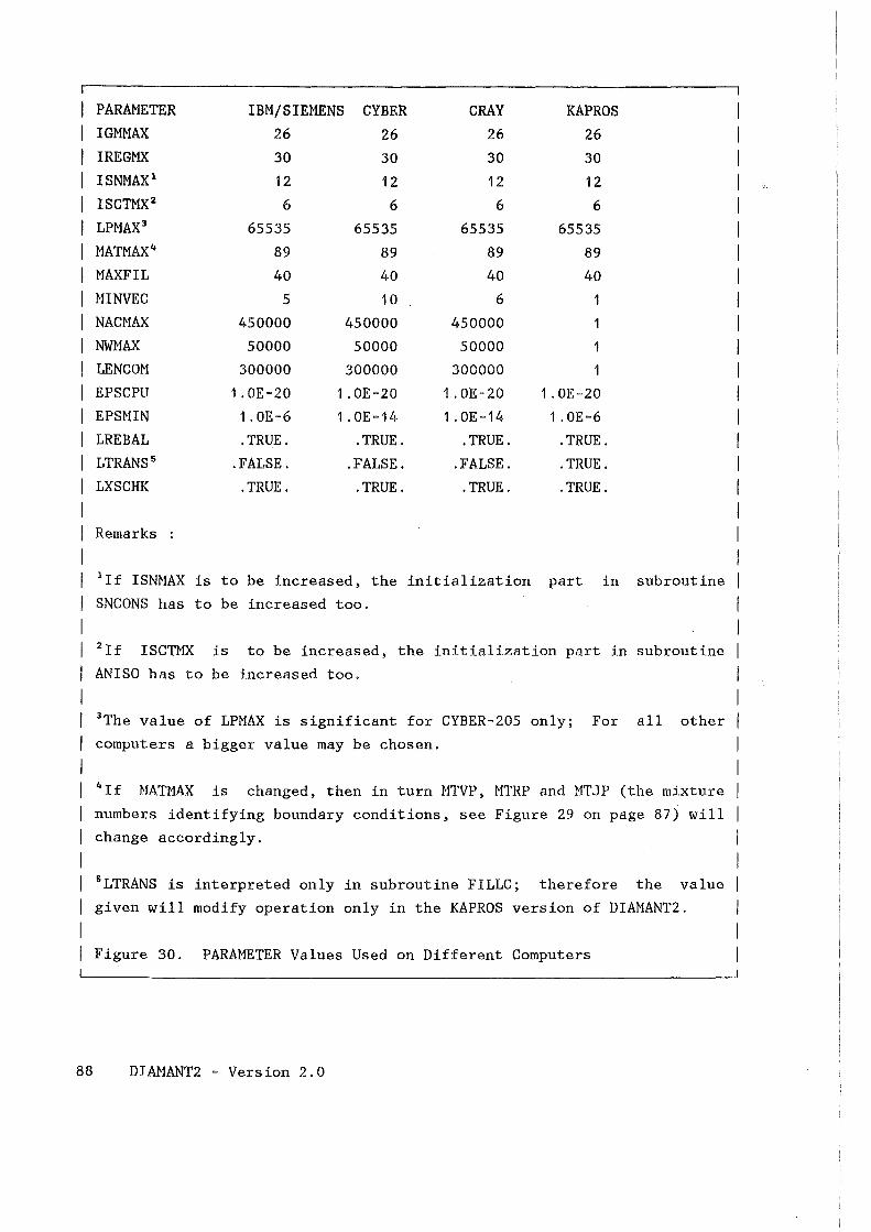
PARAMETER IBM/SIEMENS CYBER CRAY KAPROS IGMMAX 26 26 26 26 IREGr1X 30 30 30 30 ISNMAX 1 12 12 12 12 ISCTMX2 6 6 6 6 LPMAX 3 65535 65535 65535 65535 MATMAX 4 89 89 89 89 MAXFIL 40 40 40 40 HINVEC 5 10 6 NACMAX 450000 450000 450000 NWMAX 50000 50000 50000 LENCOM 300000 300000 300000 EPSCPU 1.0E-20 1.0E-20 1 .OE-20 1. OE-20 EPSNIN 1.0E-6 1 . OE-14 1 . OE -14 1. OE-6 LREBAL . TRUE. .TRUE . .TRUE. .TRUE. LTRANS 5 .FALSE. .FALSE. .FALSE. .TRUE. LXSCHK .TRUE. . TRUE. .TRUE. .TRUE .

Remarks

1 If ISNMAX is to be increased, the initialization part in subreutirre

SNCONS has to be increased too.

2 If ISCTMX is to be increased, the initialization part in subreutirre

ANISO has to be increased too.

3 The value of LPMAX is significant for CYBER-205 only; For all other

computers a bigger value may be chosen.

4 If ~1ATMAX is changed, then in turn MTVP, MTRP and MTJP (the mixture

numbers identifying boundary conditions, see Figure 29 on page 87) will

change accordingly.

5 LTRANS is interpreted only in subreutirre FILLC; therefore the value

given will modify operation only in the KAPROS version of DIAMANT2.

Figure 30. PARAMETER Values Used on Different Computers


4.6 TUNING BINARY INPUT/OUPUT

Scratch units NFANI1 and NFANI2 were needed in the old version in all

applications using anisotropic scattering expansion irrespective of the

amount of main memory available. Therefore, we have introduced a new COMNON

block /COMMOH/ serving as a container array for the data being moved from

and to NFANI1 and NFANI2. The size of this block is determined by specifying

the PARMiETER value LENCON. Automatie transition is made from disk I/0 to

storage in COMHON /COMMON/ whenever the space reserved there (PARAMETER

LENCON) is sufficient to hold all the data. Using /COMMOM/ instead of disks

saves I/0 overhead. An informative message is issued whenever LENCOM is big

enough to avoid disk I/0.

On a distinct computer there usually exist even more powerful methods to tune

I/0 (i.e. implicit I/0 on a CYBER-205 or using on IBM NVS/XA systems so

called Virtual Input Output scratch datasets which can be located in the

extended address area and are very cheap and fast in access), but these

methods are not portable.


CHAPTER 5. KAPROS SHORT DESCRIPTION OF MODULE DIAMANT2

l.PROGRAN IDENTIFICATION DIAMANT2 (VERSION 2.0) /1/

A MULTIGROUP NEUTRON TRANSPORT CODE IN REGULAR TRIANGULAR GEOHETRY

2 .COMPUTER FOR WH ICH THE PROGRAM IS DESIGNED AND OTHERS ON TYHICH IT IS OPERABLE

IBM/370, IBM30xx, SIEMENS 7. 8xx, FUJITSU FACOM 380, CYBER-205, CRAY-1,

CRAY-XMP, SIEMENS VP SERIES, FUJITSU VP SERIES, IBM3090-VF SERIES.

3.DESCRIPTION OF FUNCTION

DIAMANT2 SOLVES THE TWO-DH1ENSIONAL STATIC MULTIGROUP NEUTRON TRANSPORT

EQUATION IN PLANAR REGULAR TRIANGULAR GEOMETRY. BOTH REGULAR AND ADJOINT,

INHOMOGENEOUS AND HOMOGENEOUS PROELENS SUBJECT TO VACUUM, REFLECTIVE OR

INPUT SPECIFIED BOUNDARY FLUX CONDITIONS ARE SOLVED. ANISOTROPY IS ALLOVlED

FOR THE SCATTERING SOURCE. VOLUME AND SURFACE SOURCES ARE ALLOWED FOR

INHOMOGENEOUS PROBLEMS.

4.METHOD OF SOLUTION

THE DISCRETE ORDINATES APPROXIMATION FOR THE ANGULAR VARIABLE IS USED IN

FINITE DIFFERENCE FORH WHICH IS SOLVED WITH A DIANOND DIFFERENCE APPROXI

NATION. SPATIAL DISCRETIZATION IS PERFORHED ON A MESH, COMPOSED OF EQUILA

TERAL TRIANGLES. NEGATIVE FLUXES ARE ELININATED BY A STEP SCHE~1E ALGORITHM.

STANDARD INNER (\VITHIN-GROUP) ITERATIVE CYCLES ARE ACCELERATED BY GLOBAL

REBALANCING.

S.RESTRICTIONS

VARIABLE DU1ENSIONING IS USED SO THAT ANY COMBINATION OF PROBLEM PARAMETERS

LEADING TO A WORKING ARRAY LESS THAN NCMAX CAN BE ACCOMODATED. ON ~!OST COM

PUTERS, NCMAX CAN BE AS LARGE AS SOME HUNDRED THOUSAND WORDS. THE REMAINING

MAXIMUM VALUES ARE SPECIFIED BY A PARAMETER STATEMENT AND CAN EASILY BE

CHANGED.

Chapter 5. KAPROS Short Description of Module DIAMANT2 91

6.PARTICVLARITIES OF THE PROGRAN

THE CODE IS WRITTEN IN FORTRAN 77 (ANSI X3.9-1978). QUADRATURE SETS ARE TAILORED TO REGULAR TRIANGULAR GEOMETRY/2/. PROVISION IS MADE FOR CREATION OF INfERFACE OUTPUT FILES FOR ANGULAR INTEGRATED FLUXES AND ANGULAR FLUXES. THESE INTERFACE FILES CAN EASILY BE APPLIED IN PERTURBATION CALCULATIONS, E.G., BY THE TPTRIA CODE/4/. ALL BINARY INPUT/OUTPUT-OPERATIONS ARE LOCALIZED IN THE SUBROUTINE PACKAGE READKO. EDIT OPTIONS AND DUHP AND RESTART CAPABILITIES ARE PROVIDED. DIAMANT2 IS DESIGNED TO BENEFIT FROM VECTOR-COMPUTERS AS HUCH AS POSSIBLE.

7.MACHINE REQVIREMENTS

UP TO FOUR SCRATCH UNITS, UP TO THREE INTERFACE UNITS (USE OPTIONAL) AND THE SYSTEM INPUT/OUTPUT UNITS ARE REQUIRED. A LARGE NE~10RY IS DESIRABLE, BUT IT CAN BE REPLACED TO SOME EXTEND BY DISK OR TAPE STORAGE (THE TRANSITION IS MADE AUTOMATICALLY).

B.RELATED PROGRAMS

DIANANT2/1/ IS AN INPROVED VERSIONBASEDON THE PREVIOUS DIAMANT PROGRAM/3/. MANY COHMENTS WERE ADDED AND SU!PLIFIED PROGRAMHING WAS PERFORHED TO MAKE DIAHANT2 AS EASY TO UNDERSTAND AS POSSIBLE. AN INTERFACE FILE CAN BE CREATED FOR THE TRANSPORT PERTURBATION CODE TPTRIA /4/. A SPECIAL INPUT CHECK MODULE IS PROVIDED ALONG WITH DIAHANT2.

9.MATERIAL AVAILABLE

SOURCE DECK OF DIAMANT2 AND INPUT CHECK MODULE DIAPRD IN UPDATE FORMAT, TEST PROBLEMS INPUT, RESULTS OF EXECUTED TEST PROBLEMSAND THIS REPORT (KFK4233).

JO.REFERENCES

/1/ K.KUEFNER, J.BURKHARD, R.HEGER, "AN UPDATED FORTRAN77 VERSION OF THE 2-D NEUTRON TRANSPORT CODE DIAMANT2 FOR TRIANGULAR MESHES", KFK 4233, KARLSRUHE 1987 /2/ K.KUEFNER, B.DELMARMOL, G.MINSART, "CONTINUOUS FOUR POINT TRIANGULAR MESH DIFFERENCE SCHEMES FOR THE MULTIGROUP NEUTRON TRANSPORT EQUATION", PROC. TOP. MEETING ON COMPUTATIONAL METHODS, WILLIAMSBURG 1979


/3/ K.KUEFNER, R.HEGER, "DIAMANT2, EIN MULTIGRUPPEN NEUTRONENTRANSPORT

PROGRAMM FUER DREIECKS- UND HEXAGONALGEOMETRIE", KFK 3033, KARLSRUHE 1980

/4/ K.KOBAYASHI, G.BUCKEL, K.KUEFNER, "TPTRIA, A COMPUTER PROGRAM FOR THE

REACTIVITY AND KINETIC PARMIETERS FOR TWO-DU1ENSIONAL TRIANGULAR GEOMETRY

BY TRANSPORT PERTURBATION THEORY", KFK 4116, KARLSRUHE 1986

/5/ G. BUCKEL, \V. HOEBEL, "DAS KARLSRUHER PROGRAM~tsYSTEM KAPROS, TEIL 1 ",

KFK 2253, KARSRUHE 1976

11.PROGRANNING LANGVAGE USED

STANDARD FORTRAN 77 PLUS SYSTEM DEPENDENT TIMING ROUTINES

12.0PERATING SYSTEM/MONITOR UNDER WHICH PROGRAN IS EXECUTED

IBN HVS/XA, CDC VSOS, GRAY COS, SIEMENS BS3000

COMPILER: SIEHENS-FORTRAN77, IBH-VS-FORTRAN, CYBER-FTN200, CRAY-CFT

13.ANY OTHER PROGRANHING OR OPERATING INFORMATION

THIS CODE \VAS DESIGNED TO RUN UNDER CONTROL OF THE MODULAR CODE SYSTEM KAPROS

/5/ BUT USE AS STAND ALONE CODE IS EASILY POSSIELE. IT IS DESIRABLE TRAT

THE TH1ING FUNCTIONS TASKTI AND TIMLU1 COULD BE REPLACED BY SONE SYSTEM

DEPENDENT TH1ING ROUTINE (AVAILABLE FOR: IBM, CYBER, GRAY, FUJITSU/SIEHENS).

14.NANE AND ESTABLISHMENT OF AUTHORS

KLAUS KUEFNER, JUERGEN BURKHARD, RENATE HEGER

NUCLEAR RESEARCH CENTER KARLSRUHE / INR

P. 0. BOX 3640

D-7500 KARLSRUHE

FEDERAL REPUBLIC OF GERHANY

Chapter 5. KAPROS Short Description of Module DIAMANT2 93

CHAPTER 6. INPUT DESCRIPTION

6.1 GENERAL REMARKS

DIAMANT2 reads all input cards from logical unit 14. For the KAPROS version

this unit is realized as a datablock DBN=DIAHANT25EINGABE as shown in "KAPROS

Version" on page 127.

Each K. stands for one logical record of the input stream. Each S. marks a 1 1

logical branching point in the otherwise sequential input. All variables are

to be input according to the KAPROS input conventions /4/ or, for the

stand-alone version, according to the rules of FORTRAN list-directed input

/15/. Note also the remarks at the end of this chapter where explanations

for special options are given.

All explanations given in the following are valid fo.r the real problern. They

apply usually as well to adjoint problems, exceptions from this rule are

specially indicated.

All maximum values can be changed by inserting new bounds in the PARMiETER

statement and recompiling the code (see Figure 29 on page 87). The maximum

value allowed for the mixture number (=89), the number used to identify

vacuum (=90), reflective (=91) or boundary flux (=92) boundary conditions

are all fixed by the value of the PARMiETER MATMAX and can easily be changed.

Chapter 6. Input Description 95

6.2 INPUT CARD SEQUENCE

KJ: Identification label of the run (60 characters)

(enclosed in apostrophes within KAPROS)

K2: (integer control data)

ID:

ITH:

ISN:

I GM: IEVT:

MLM:

MCM:

MT:

MAT:

ICM:

Identification number of the run (not used in this version)

Theory option and selector for perturbation file option

O=Real calculation without creation of perturbation theory file

1=Adjoint calculation without creation of perturbation theory

file

-1=Adjoint calculation with creation of perturbation theory

file

-2=Real calculation with creation of perturbation theory file

Order of the angular discretization (ISN has to be even and

mod(ISN,100) ~ 12) and selector of quadrature set:

2, ... ,12 use PN set

102, ... ,112 use DPN set of order ISN- 100

202, ... ,212 use EPN set of order ISN- 200

Number of energy groups (maximum allowed 26)

Problem type (0: External source problem, 1: Eigenvalue prob

lern)

Number of intervals on the oblique side of the reference

parallelegram

Number of intervals on the horizontal side of the reference

parallelegram

Number of mixtures to be used (maximum allowed : 89)

Number of cross section-tables to be stored (maximum allowed :

89; MAT = HT for isotropic cases, MAT ~ MT for anisotropic

cases). How MAT is tobe calculated is shown in "How to Specify

Anisotropie Mixtures" on page 110.

Maximum number of outer iterations (see "How to Choose Iter

ation Control Parameters" on page 79)

11M: Maximum number of inner iterations (see "How to Choose Iter

ation Control Parameters" on page 79)


lll:

KTR:

KDUM:

NFPERT:

NFDMPN:

NFDMPO:

INBO:

II

Starting number of inner iterations (see "How to Choose Iter-

ation Control Parameters" on page

Control of neutron flux print

fluxes to be printed)

79)

(-1/0/1 All/None/Seleeted

Cross section input by cards (=0: No, SIGHN block used; =1: Yes)

FORTRAN unit for interface file to perturbation module

(see "Data Files Used" on page 63).

Final flux to be written on this unit

=0 Not used

>0 FORTRAN unit number of data set

(see "Data Files Used" on page 63).

Initial flux to be read from this unit

=0 Not used

>0 FORTRAN unit number of data set

(see "Data Files Used 11 on page 63).

Control of boundary flux option (see "Boundary Fluxes" on page

112) .

=0: No boundary flux,

=1: boundary flux by group and interval,

=2: by energy spectrum and source strength

jS1 I If no flux guess is used (NFDNPO = 0 on K2) continue with K4 L__j

K3: (flux guess map selection)

NUMFL:

IDFL:

Position number of the flux guess map on data file NFDHPO which

is to be used

Identification number of the run that created the flux guess

(variable not used in this version)


K4: (integer control data continued)

I QUELL:

MBK:

IQUER:

101:

102:

103:

104:

105:

ISCT:

KAUSW:

Distributed source option indicator (see remark on "External

Sources" on page 1 '12).

=0: No distributed source

=1: Given by triangle and group

=-1: Given by mixture and group

=2: Given by spectrum and source strength for each triangle

=-2: Given by spectrum and source strength for each mixture

Buckling correction option

=0: No buckling term

=1: Constant value given on input card KS

=2: Group dependent values

=3: Group and mixture dependent values

Print cross section tables; (=0: No, =1: Yes)

Reaction rates or densities for fission cross section

(0/1/2 : None/Density/Rate)

Reaction rates or densities for capture cross section


Reaction rates or densities for absorption cross section


Reaction rates or densi ties for fission neutron production

cross section


Reaction rates or densities for total cross section


Note: ID1 - IDS are edit options for evaluation purposes. If

chosen different from zero they create printed output but no

data are written on the interface file.

Anisotropie scattering order

=0: Isotropie, maximum allowed: 6

Neutron balances selector

=0: Global balances only

=1 : Global balances and regionwise balances

=10: Global balances and mixture dependent balances

=11: Global, regionwise and mixture dependent balances


NFANI1:

NFSCRl:

I NORM:

Note: KAUSW is only an edit option for evaluation; but group

wise total fluxes may be transfered to the perturbation inter

face file NFPERT (see "Data Files Used" on page 63).

FORTRAN unit for anisotropy working set (see "Data Files Used"

on page 63)

FORTRAN unit for auxiliary working set in storage optimization

2 (see "Data Files Used" on page 63 and "Storage Optimization

Levels" on page 65)

Flux normalization selector (see "Niscellaneous" on page 114)

=1: normalization to one fission event

=2: normalization to power = 1 Watt

KS: (real control data)

EPS:

EV: BF:

H: EPSA:

TEPS:

Convergence criterion for termination of outer iterations

< 0: integral test using eq. (38)

= 0: eigenvalue bounds test using value of TEPS and eqs. (40)

> 0: pointwise test using eq. (39)

Starting guess for eigenvalue (not relevant for IEVT=O)

Buckling height (Used if NBK = 1 on card K4)

Length of triangle side (in cm)

Convergence test selector for inner iterations

< 0: integral test using eq. (33) ·

= 0: integral test using eq. (33) with EPS for EPSA

> 0: pointwise test using eq. (34)

Convergence criterion for termination of outer iterations if

eigenvalue bounds are requested (EPS = 0.0)

K6: (not read in this version)


Kl: (mixture numbers used and anisotropy selector)

MATTAB:

KB:

ITYP:

IZEI:

ISPA:

MISCH:

INTZ:

INTS:

MT (see K2) integer numbers to specify mixtures with aniso

tropic scattering kerne! expansion. These mixtures are indi

cated by a negative sign in front of the mixture number. (see

"How to Specify Anisotropie Mixtures" on page 11 0 and the

example given there).

Additionally, it is possible within KAPROS to apply the HATTAB

input for selecting certain mixtures out of a SIGMN-block (see

"Nuclear Cross Section Input by SIGMN Block" on page 107 and

the example given there). Thereby one can avoid storing

cross-section data which are not relevant for the DIAHANT2

calculation but may be needed in subsequent perturb~tion cal

culations.

Input of the mixture distribution by means of overlapping basic

zones (zones with uniform mixture, see "Mixture Distribution"

on page 106); if several basic zones are overlapped, the last

value entered applies. This card has tobe repeated until the

model is completely specified.

Type of basic zone, see Figure 31 on page 101.

Grid line number for the left upper corner of the basic zone

Grid column number for the left upper corner; the left upper

corner of the reference parallelegram is ISPA = IZEI = 0

Mixture number assigned to the basic zone (see note below and

"How to Specify Anisotropie Hixtures" on page 11 0 and the

example given there).

number of line intervals of the basic zone

Number of column intervals of the basic zone

Note: Boundary conditions are specified by the mixture distribution input

using mixture numbers 90 (=vacuum), 91 (=reflection) or 92 (=boundary flux).

These numbers are fixed in a PARAMETER statement and can easily be changed.

r-,

IS21 If mixture input is complete continue with KBA, otherwise K8 again L_j


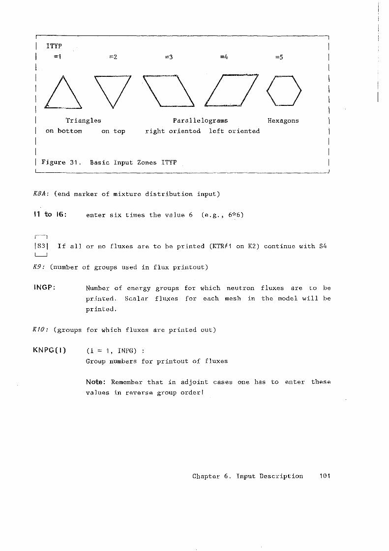
ITYP

=1 =2 =3 =4 =5

Triangles Parallelegrams Hexagons

on bottom on top right oriented left oriented

Figure 31. Basic Input Zones ITYP

KBA: (end marker of mixture distribution input)

11 to 16: enter six times the value 6 (e.g., 6*6)

,----, IS31 If all or no fluxes are tobe printed (KTR~1 on K2) continue with S4 L__j

K9: (number of groups used in flux printout)

INGP: Number of energy groups for which neutron fluxes are to be

printed. Scalar fluxes for each mesh in the model will be

printed.

KlO: (groups for which fluxes are printed out)

KNPG(I) (I = 1, INPG)

Group numbers for printout of fluxes

Note: Remernher that in adjoint cases one has to enter these

values in reverse group ordert


II

IS41 L._j

If cross section input is by SIGMN block (KDUM = 0 on K2) continue

with SS Note:Cross section input sequence is the same for real and

adjoint problems; the necessary changes are made automatically by DIAMANT2.

KJJ: (fission spectrum input)

CHI( I) (I = 1, IGM) :

Input of values for the fission spectrum (assumed to be mix

ture-independent).

For K = 1, MAT (MAT see input card K2)

K12: (nuclear cross sections matrix)

C(I,J,K) ((I= 1, IHM), J = 1, IGM)

II

Input of the nuclear cross sections (IHN = IGM + IHT; arrange

ment of the cross sections see "Card Input of Nuclear Cross

Sections" on page 110 and Figure 34 on page 109)

ISS! For NBK < 2 (see input card K4) continue with S7 L__j

II

IS61 L__j

For NBK = 2 (see input card K4) continue with K14A

For NBK = 3 (see input card K4) continue with K14B

K14A: (buckling values)

B(K) (K = 1, IGM)

Group-dependent buckling values (mixture-independent)


values in reverse group order!


K14B: (buckling values)

B(J,K) ((J = 1, MT), K = 1, IGM) :

r-1

Hixture and group-dependent buckling values


values in reverse group order!

IS71 If no external source input (!QUELL= 0 on K4) continue with 88 L~.J

If !QUELL = (input dependent on meshes and energy group)

continue with K15A

If !QUELL= 2 (input dependent on meshes; source equal to product

of spectrum times source strength) continue with K15B

If !QUELL =-1 (input dependent on mixtures and energy group)

continue with K15C

If !QUELL =-2 (input dependent on mixtures; source equal to product

of spectrum times source strength) continue with K15D

Notes: See "External Sources" on page 112 at the end of this chapter for a

discussion of the special type of external source input and definition of

input values.

Remernher that in adjoint cases one has to enter these values in reverse group

order!

K15A: (external source input)

For K ""' 1, IGH

QHI): ML records with MC(ML1) values for the external source of each

triangle

Note: See "External Sources" on page 112 at the end of this

chapter for the definition of the variables ML, ML1 and HC (HL1).

Continue with 88


K15B: (external source input)

Q2(K):

Ql(l):

(K = 1,IGM)

!GM values with the spectrum for the external source

ML records with MC(ML1) values for the external source strength

of each triangle

Note: See 11External Sources 11 on page 112 at the end of this

chapter for the definition of the variables ML, ML1 and MG (ML1).

Continue with S8

K15C: (external source input)

For K = 1, IGM

Q3(J, K) (J = 1, HT) :

values of the source strength for each mixture; one record for

each energy group.

Continue with S8

K15D: (external source input)

Q2(K): IGH values with the spectrum of the external source

MT values of the source strength for each mixture Q3(J):

r----1

jS8l If no boundary flux (INBO=O on input card K2) continue with K17 L_j

If INBO = continue with K16A

If INBO = 2 continue with K16B

Notes: See 11 Boundary Fluxes 11 on page 112 at the end of this chapter for a

discussion of the special type of boundary flux input and definition of input

values.

Remernher that in adjoint cases one has to enter these values in reverse group

order!


K16A: (boundary flux input)

For K = 1 , IGM :

For J = 1, NB

BND(J 1 11 K) (I= 1, NI(J)) :

values for the boundary flux

Note: See "Boundary Fluxes" on page 112 at the end of this

chapter for the definition of the variables NB and NI.

Continue with K17

K16B: (boundary flux input)

BND( 1 11 1 K): IGM values with the spectrum of the boundary fluxes

K16C:

For J = 1, NB :

BND(J I I I 1): (I = 1' NI (J))

values for the source strength

Note: See "Boundary Fluxes" on page 112 at the end of this

chapter for the definition of the variables NB and NI.

K17: (end of problern input)

CKK: Four bytes character constant

= ENDE : End of DIAMANT2 input

= CONT : Input for additional case starting from K1

(enclosed in apostrophes within KAPROS)

For the KAPROS version the END-OF-DATABLOCK marker *$*$ completes the whole

input sequence.


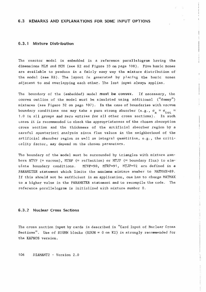
6.3 REMARKS AND EXPLANATIONS FOR SOME INPUT OPTIONS

6.3. 1 Mixture Distribution

The reactor model is embedded in a reference parallelegram having the

dimensions MLM and NCM (see K2 and Figure 33 on page 108). Five basic zones

are available to produce in a fairly easy way the mixture distribution of

the model (see K8). The layout is generated by placing the basic zones

adjacent to and overlapping each other. The last input always applies.

The boundary of the (embedded) model must be convex. If necessary, the

convex outline of the model must be simulated using additional (''dummy")

mixtures (see Figure 32 on page 107). In the case of boundaries with vacuum

boundary conditions one may take a pure strong absorber (e.g., cr = cr. t = a t:o 1. 0 in all groups and zero entries for all other cross sections). In such

cases it is recommended to check the appropriateness of the chosen absorption

cross section and the thickness of the artificial absorber region by a

careful aposteriori analysis since flux values in the neighborhood of the

artificial absorber region as well as integral quantities, e.g., the criti

cality factor, may depend on the chosen parameters.

The boundary of the model must be surrounded by triangles with mixture num

bers MTVP (= vacuum), MTRP (= reflection) or MTJP (= boundary flux) to sim

ulate boundary conditions. MTVP=90, MTRP=91 , MTJP=92 are defined in a

PARAMETER statement which limits the maximum mixture nurober to MATMAX=89.

If this should not be sufficient in an application, one has to change HATMAX

to a higher value in the PARAMETER statement and to recompile the code. The

reference parallelegram is initialized with mixture nurober 0.

6.3.2 Nuclear Cross Sections

The cross section input by cards is described in "Card Input of Nuclear Cross

Sections". Use of SIGMN blocks (KDUM = 0 on K2) is strongly recommended for

the KAPROS version.


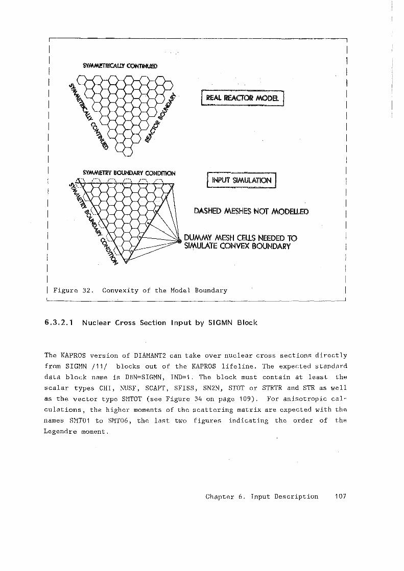
[ REAL Rf.ACTOI MOoa I

I INPUT SIMULATION I

DASHED MESHES NOT MODEtlED

Figure 32. Convexity of the Model Boundary

I I I I I I I I I I I I I I I I I I I I I I I

L_----------------------------------------------------------------~

6.3.2.1 Nuclear Cross Section Input by SIGMN Block

The KAPROS version of DIAMANT2 can take over nuclear cross sections directly

from SIGMN /11/ blocks out of the KAPROS lifeline. The expected standard

data block name is DBN=SIGMN, IND=1. The block must contain at least the

scalar types CHI, NUSF, SCAPT, SFISS, SN2N, STOT or STRTR and STR as well

as the vector type SMTOT (see Figure 34 on page 109). For anisotropic cal

culations, the higher moments of the scattering matrix are expected with the

names SMT01 to SMT06, the last two figures indicating the order of the

Legendre moment.


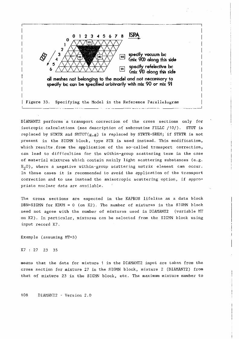
0 1 2 3 4 5 6 7 8

spedfy vacuum bc (mix 90> along this side

[!!] speclfy refelectlve bc (mix 91) along this side

oll meshes not belonging to the model and not neccessary to specify bc can be specified arbitrarily with mix 90 or mlx 91

Figure 33. Specifying the Model in the Reference Parallelegram

DIAHANT2 performs a transport correction of the cross sections only for

isotropic calculations (see description of subroutine FILLC /10/). STOT is

replaced by STRTR and SNTOT(g,g) is replaced by STRTR-SREH; if STRTR is not

present in the SIGHN block, type STR is used instead. This modification,

which results .from the application of the so-called transport correction,

can lead to difficulties for the within-group scattering term in the case

of material mixtures which contain mainly light scattering substances (e.g.

H20), where a negative within-group scattering matrix element can occur.

In those cases it is recommended to avoid the application of the transport

correction and to use instead the anisotropic scattering option, if appro

priate nuclear data are available.

The cross sections are expected in the KAPROS lifeline as a data block

DBN==SIGNN for KDUH = 0 (on K2). The number of mixtures in the SIGHN block

need not agree with the number of mixtures used in DIAHANT2 (variable NT

on K2). In particular, mixtures can be selected from the SIGMN block using

input record K7.

Example (assuming HT=3)

K7 : 27 23 35

means that the data for mixture 1 in the DIAHANT2 input are taken from the

cross section for mixture 27 in the SIGHN block, mixture 2 (DIAHANT2) from

that of mixture 23 in the SIGHN block, etc. The maximum mixture number to


~------~------~------------------------------~1 k C(k,i,j) Explanation II

~------+-------~--------------------------------~1 IPSFIS fission cross section II

~------+-------~----~--------------------------~1 IPSCAP capture cross section II 0 capt

r-------r-------r-------------------------------~1

IPSN2N 0 n,2n (n,2n) cross section II ~------+-------~--------------------------------~1

IPSTR transport cross section II ~------+-------~--------------------------------~1

IHT-2 absorption cross section II r-------~------+---------------------------------~1

IHT-1 fission production cross section II ~------4--------+----------------------------------~l

IHT total cross section II r-------~------+---------------------------------~1

og4 g within-group scatter cross section I I r-------~------+---------------------------------~1

IHS

IHS+1

down-scatter cross section

IHM

II II II

~------~------~----------------------------------~1

Remarks:

1 . Indices i = energy group and j

ranges: i=1 to IGM and j=1 to MAT.

I I I

= mixture nurober have the following I I I

2. No up-scattering and full down-scattering is assumed (IHS = IHT+1, I I I

IHM = IHT+IGM)

Figure 34. Storage Sequence in Cross Section Array C I

be used in DIAMANT2 (defined in a PARAMETER statement) is 89 (90, 91 and 92

are reserved to define boundary conditions, see "Mixture Distribution" on

page 106).


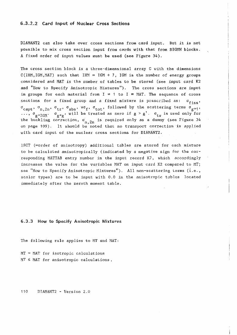
6.3.2.2 Card Input of Nuclear Cross Sections

DIAHANT2 can also take over cross sections from card input. But it is not

possible to mix cross section input from cards with that from SIGMN blocks.

A fixed order of input values must be used (see Figure 34).

The cross section block is a three-dimensional array C with the dimensions

C (IHM, IGM, ~1AT) such that IH~f = IGM + 7, Imf is the number of energy groups

considered and MAT is the number of tables to be stored (see input card K2

and "How to Specify Anisotropie Mixtures"). The cross sections are input

in groups for each material from I = 1 to I = MAT. The sequence of cross

sections for a fixed group and a fixed mixture is prescribed as: Clf. , 1SS

Clcapt' on, 2n' Cltr' Clabs' vof' Cltot' followed by the scattering terms og~ 1 ,

... , o g-'*IGW o g~g 1 will be treated as zero if g > g 1 • otr is used only for

the buckling correction, Cl 2 is required only as a dummy (see Figure 34 n, n on page 109). It should be noted that no transport correction is applied

with card input of the nuclear cross sections for DIAMANT2.

ISCT (=order of anisotropy) additional tables are stored for each mixture

to be calculated anisotropically (indicated by a negative sign for the cor

responding HATTAB entry nurober in the input record K7, which accordingly

increases the value for the variables MAT on input card K2 compared to NT;

see "How to Specify Anisotropie Mixtures"). All non-scattering terms (i.e.,

scalar types) are to be input with 0.0 in the anisotropic tables located

immediately after the zeroth moment table.

6.3.3 How to Specify Anisotropie Mixtures

The following rule applies to MT and MAT:

MT = HAT for isotropic calculations

MT :5 HAT for anisotropic calculations .


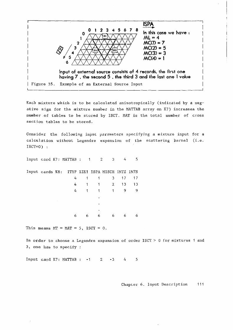
0 1 2 3 ~ ' 6 7 8 ISPA ___... ln this case we have : Ml 1111 4 MCC1> 11117

MCC2> 1111 5 MC<3> 1111 3 MCC4) • 1

Input of external source c:onslsts of 4 rec:ords, the first one having 7 , the sec:ond 5 , the third 3 and the last one 1 value

Figure 35. Example of an External Source Input

Each mixture which is to be calculated anisotropically (indicated by a neg

ative sign for the mixture number in the HATTAB array on K7) increases the

number of tables to be stored by ISCT. NAT is the total number of cross

section tables to be stored.

Consider the following input parameters specifying a mixture input for a

calculation without Legendre expansion of the scattering kernel (i.e.

ISCT=O) :

Input card K7: MATTAB 2 3 4 5

Input cards K8: !TYP IZEI ISPA HISCH INTZ INTS

4 1 3 1 7 1 7

4 2 13 13

4 9 9

6 6 6 6 6 6

This means NT = MAT = 5, ISCT = 0.

In order to choose a Legendre expansion of order ISCT > 0 for mixtures 1 and

3, one has to specify

Input card K7: MATTAB -1 2 -3 4 5


Input cards K8: remain unchanged I

This means MT= 5, and because we have two anisotropic mixtures, HAT= MT+

2*ISCT and ISCT > 0. Note that the same order of Legendre expansion (ISCT)

is used for all mixtures. In additiontothat small input change, now more

nuclear cross sections have to be provided and the file numbers for scratch

units NFANI1 and NFANI2 on input card K4 must have meaningful values.

6.3.4 Externat Sources

The following section refers to input cards K15A and K15B used to specify

an external source input (see Figure 35).

ML is the total number of grid lines which pass through the real model (the

reference parallelegram contains MLM grid lines; the real model is marked

as thick lined triangle in Figure 35 on page 111), and MC(ML1) is the number

of triangles which are contained in line ML1 of the model (the reference

parallelegram contains 2*MCM triangles per line). The model must be swept

completely, beginning with the upper left triangle and working to the right.

Once a line has been completed, input continues with the next lower line.

In preparing input for external source problems, a user should take care of

the influence of reflective boundary conditions if only a sector of the

reactor is specified; i.e., he should be aware that at symmetrical positions

there will exist equivalent external Sources which contribute to the total

source strength inserted into the whole reactor.

The user should also be aware of having specified the appropriate physical

dimension for the external source. In the real case, evidently the external

source should have the dimension of fission sources. This means, e.g., that

the dimension of the source strength has to be compatible with the production

rate (i.e., neutrons per cm 3 s) and the corresponding energy spectrum with

the fission spectrum.

112 DIAMANT2 -Version 2.0

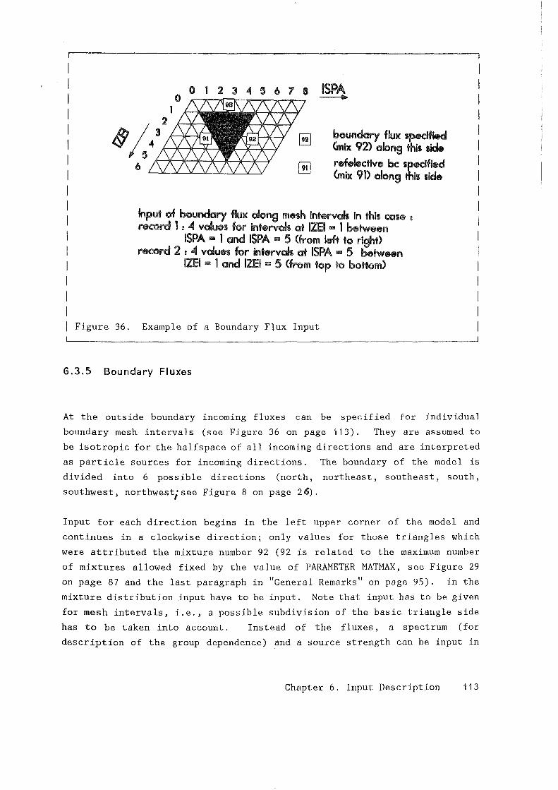
I I I I I I I I I I I I I I I I I I Figure 36.

0 I 2 3 4 5 6 7 8 ISPA _____...

boundary flux speafied Cmix 92) along this Iide refelectlve bc spedfied Cmix 91) along this side

Input of boundary flux along mesh intervak in this case : record 1 : ~ vabts for intervak at IZ8 • 1 between

ISPA = 1 and ISPA = 5 Cfrom left to rlght> record 2 : ~ vdues for intervak at ISPA • 5 between

IZ8 = 1 and IZEI = 5 (from top to bottom)

Example of a Boundary Flux Input

6.3.5 Boundary Fluxes

At the outside boundary incoming fluxes can be specified for individual

boundary mesh intervals (see Figure 36 on page 113). They are assumed to

be isotropic for the halfspace of all incoming directions and are interpreted

as particle sources for incoming directions. The boundary of the model is

divided into 6 possible directions (north, northeast, southeast, south,

southwest, northwest;see Figure 8 on page 26).

Input for each direction begins in the left upper corner of the model and

continues in a clockwise direction; only values for those triangles which

were attributed the mixture number 92 (92 is related to the maximum number

of mixtures allowed fixed by the value of PARAMETER MATMAX, see Figure 29

on page 87 and the last paragraph in "General Remarks" on page 95). in the

mixture distribution input have tobe input. Note that input has to be given

for mesh intervals, i.e., a possible subdivision of the basictriangle side

has to be taken into account. Instead of the fluxes, a spectrum (for

description of the group dependence) and a source strength can be input in


the sequence described above (INBO = 2). In the latter case, boundary fluxes

are calculated as the product of spectrum times source strength.

In preparing input for boundary flux problems, a user should take care of

the influence of reflective boundary conditions if only a sector of the

reactor is specified; i.e., he should be aware that at symmetrical positions

there will exist equivalent boundary fluxes which contribute to the total

boundary flux acting on the whole reactor. In the real case, evidently the

boundary flux should correspond to angular fluxes. For the adjoint problem,

the specification concerns outgoing adjoint fluxes at the boundary according

to "Adjoint Calculations" on page 23.

6.3.6 Miscellaneous

• The following constraints apply to all optional data file numbers

I < 40. and I ~ 5,6,14;

Corresponding operating system cards have to define the files used

beforehand. Within KAPROS, some of the files may be realized as KAPROS

datablocks and may require then a •'~KSIOX card (see "KAPROS Version" on

page 127).

• All data files used by DIAMANT2 must be defined within KAPROS in a

separate data block with name INITDREAD5DIAMAN (see "KAPlWS Implementa

tion" on page 69 and Figure 24 on page 71).

• In normalizing power in a calculation (INOR~f = 2 on K4) it is assumed

that the power portion proportional to the neutron flux is approximately

200 NeV per fission event. The user must take into account the reactor

section (because of symmetries) to which the normalization applies.


CHAPTER 7. SAMPLE OUTPUT INTERPRETATION

This is a description of the printed output of a DIAMANT2 calculation. The

purpese of this section is to facilitate interpretation of the output for

the user (see program output in "Appendix B. Example of a DIAMANT2 Calcu

lation" on page 125).

Part 1 of the Output: Program Constants and Input Protocol

All values of the currently valid PARMfETER statement are printed and briefly

explained. Subsequently, the division of working arrays into subarrays is

printed.

Then all input values are tabulated, the discrete directions along with the

associated integration weights and the angle sweeps sequence are printed.

The directions are characterized by the direction cosines of their pro

jections in the x-y plane. The nuclear cross sections may be printed out (if

requested by inputvariable IQUER):

FISSION FRAC

GROUP SUM

CROSS SECTIONS

Fission spectrum

Group sum for all fission spectra (usually close

to 1 .0).

Nuclear cross section matrix C for each material

(including higher Legendre moments if ISCT > 0).

A message may appear beforehand if the input absorption cross section has

been replaced by a calculated one. For the KAPROS version some diagnostic

output from FILLC will be printed whenever cross sections are read from a

SIGHN block.

After that, the reactor model to be calculated is sketched in the printout

with heading

MIXTURE DISTRIBUTION Sketch of the mixture distribution in the refer

ence parallelegram (including boundary condi

tions)

Chapter 7. Sample Output Interpretation 115

An error message (ISTOP = 16) will appear if the mixture distribution input

will reference a mesh cell outside the reference parallelogram.

Part 2 of the Output: The Iteration Monitor

The following information is output after each outer iteration:

..

..

..

..

..

..

current outer iteration number;

total number of outer iterations;

total number of inner iterations;

criticality factor (lower estimate);

criticality factor (keff);

criticality factor (upper estimate);

outer iteration error;

mesh point indices of maximum outer error;

CPU-time used in seconds;

A special message is output if negative flux fix-up has been activated. The

following information is printed for each group (within the outer iteration

moni tor pr int) : .. .. .. .. ..

energy group considered;

number of inner iterations in this group;

inner iteration error;

mesh point indices of maximum inner error;

rebalancing factor (if rebalancing is switched on) according to Eq. (35) .

Part 3 of the Output: Results During the Final Iteration

..

..

..

..

116

information why iteration stops (convergence or maximum 'iteration count

reached or CPU time exhausted);

information on the normalization of fluxes;

global balances followed by mixture and/or region balances (if selected

by input);

various reaction rates and/or reaction densities (as selected by input);

output of the scalar fluxes ( as selected by input);

volume integrated fission source;

information if a restart dump has been created (if this option is used,

the number NUMFL under which the dump is stored will also be printed).

DIAMANT2 - Version 2.0

Part 4 of the Output: Final Iteration Result

The result of the final outer iteration is output in almost the same format

as the normal iteration monitor.

" information on the vectorlength for that case;

information on convergence criteria used;

outer iteration monitor print;

negative flux fix-up summary;

information why iteration stops (convergence or maximum iteration count

reached or CPU time exhausted);

timing statistics (including the execution speed v mentioned in "How to

Estimate Computing Time" on page 80).

If the stop code ISTOP is different from zero, a list of stop codes along

with an explanation of their meanings is added.

Chapter 7. Sample Output Interpretation 117

118 DIAMANT2 -Version 2.0

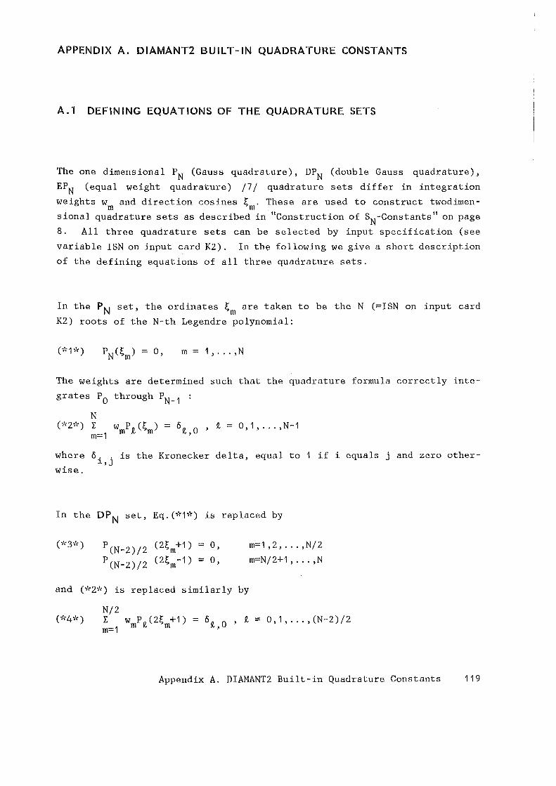
APPENDIX A. DIAMANT2 BUIL T-IN QUADRATURE CONSTANTS

A.l DEFINING EQUATIONS OF THE QUADRATURE SETS

The one dimensional PN (Gauss quadrature), DPN (double Gauss quadrature),

EPN (equal weight quadrature) /7 I quadrature sets differ in integration

weights w and direction cosines t . These are used to construct twodimen-m m sional quadrature sets as described in "Construction of SN-Constants" on page

8. All three quadrature sets can be selected by input specification (see

variableISNon input card K2). In th~ following we give a short description

of the defining equations of all three quadrature sets.

In the PN set, the ordinates ~m are taken to be the N (=ISN on input card

K2) roots of the N-th Legendre polynomial:

m = 1, ... ,N

The weights are determined such that the quadrature formula correctly inte

grates P0 through PN_ 1

N (*2*) I wmPl(~m) = öl,O , l = 0,1, ... ,N-1

m==1

where ö .. is the Kronecker delta, equal to 1 if i equals j and zero other-1,J

wise.

In the DPN set, Eq. (~""1~'r) is replaced by

and (*2*) is replaced similarly by

Nl2

m= 1 , 2 , . . . , NI 2

m=NI2+1, ... ,N

I w Pn(2~ +1) = ön 0 , l == 0,1, ... ,(N-2)12 m=1 m ~ m ~,

Appendix A. DIAHANT2 Built-in Quadrature Constants 119

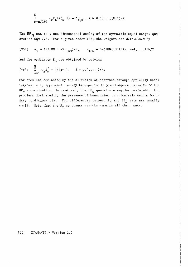
69.. 0 ' 9.. , = 0,1, ... ,(N-2)/2

The EPN set is a one dimensional analog of the symmetric equal weight qua

drature EQN /7/. Fora given order ISN, the weights are determined by

riSN = 8/(ISN(ISN+2)), m=1, ... ,ISN/2

and the ordinates ~ are obtained by solving m

N E w ~9.. = 1/(9..+1), m=1 m m

9.. = 2,4, ... ,ISN.

For problems dominated by the diffusion of neutrons through optically thick

regions, a PN approximation may be expected to yield superior results to the

DPN approximation. In cantrast, the DPN quadrature may be preferable for

problems dominated by the presence of boundaries, particularly vacuum boun

dary conditions /8/. The differences between PN and EPN sets are usually

small. Note that the s2 constants are the same in all three sets.


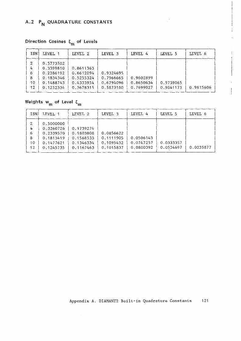
A.2 PN QUADRATURE CONSTANTS

Direction Cosines !; of Levels m -,

ISNI LEVEL 1 LEVEL 2 LEVEL 3 LEVEL 4 LEVEL 5 LEVEL 6 I

2 0.5773502 4 0.3399810 0.8611363 6 0.2386192 0.6612094 0.9324695 8 0.1834346 0.5255324 0.7966665 0.9602899 10 0. 1488743 0.4333954 0.6794096 0.8650634 0.9739065 12 0.1252334 0.367831.5 0.5873180 0.7699027 0.9041173 0.9815606

Weights w of Level ~ m m

ISNI LEVEL 1 LEVEL 2 LEVEL 3 LEVEL 4 LEVEL 5 LEVEL 6

2 0.5000000 I 4 0.3260726 0.1739274 I 6 0.2339570 0.1803808 0.0856622 I 8 0.1813419 0. 1568533 0.1111905 0.0506143 I 10 0.1477621 0.1346334 0. 1095432 0.0747257 0.0333357 I 12 0.1245735 0.1167463 0.1015837 0.0800392 0.0534697 0. 0235877 I

__j

Appendix A. DIAMANT2 Built-in Quadrature Constants 121

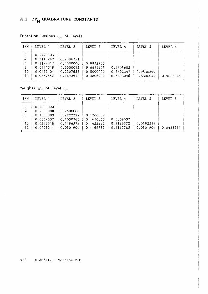
A.3 DPN QUADRATURE CONSTANTS

Direction Cosines ~m of Levels

IISN LEVEL 1 LEVEL 2 LEVEL 3 LEVEL 4 LEVEL 5 LEVEL 6

I 2 0.5773503 I 4 0.2113249 0.7886751 I 6 0.1127017 0.5000000 0.8872983 I 8 0.0694318 0.3300095 0.6699905 0.9305682 I 10 0.0469101 0.2307653 0.5000000 0.7692347 0.9530899 I 12 0.0337652 0.1693953 0.3806904 0.6193096 0.8306047 0.9662348


IISN LEVEL 1 LEVEL 2 LEVEL 3 LEVEL 4 LEVEL 5 LEVEL 6

2 0.5000000 I 4 0.2500000 0.2500000 I 6 0.1388889 0.2222222 0. 1388889 I 8 0.0869637 0. 1630363 0.1630363 0.0869637 I 10 0.0592318 0.1196572 0.1422222 0.1196572 0.0592318 I 12 0.0428311 0.0901904 0.1'169785 0.1169785 0.0901904 0.0428311 I

_j


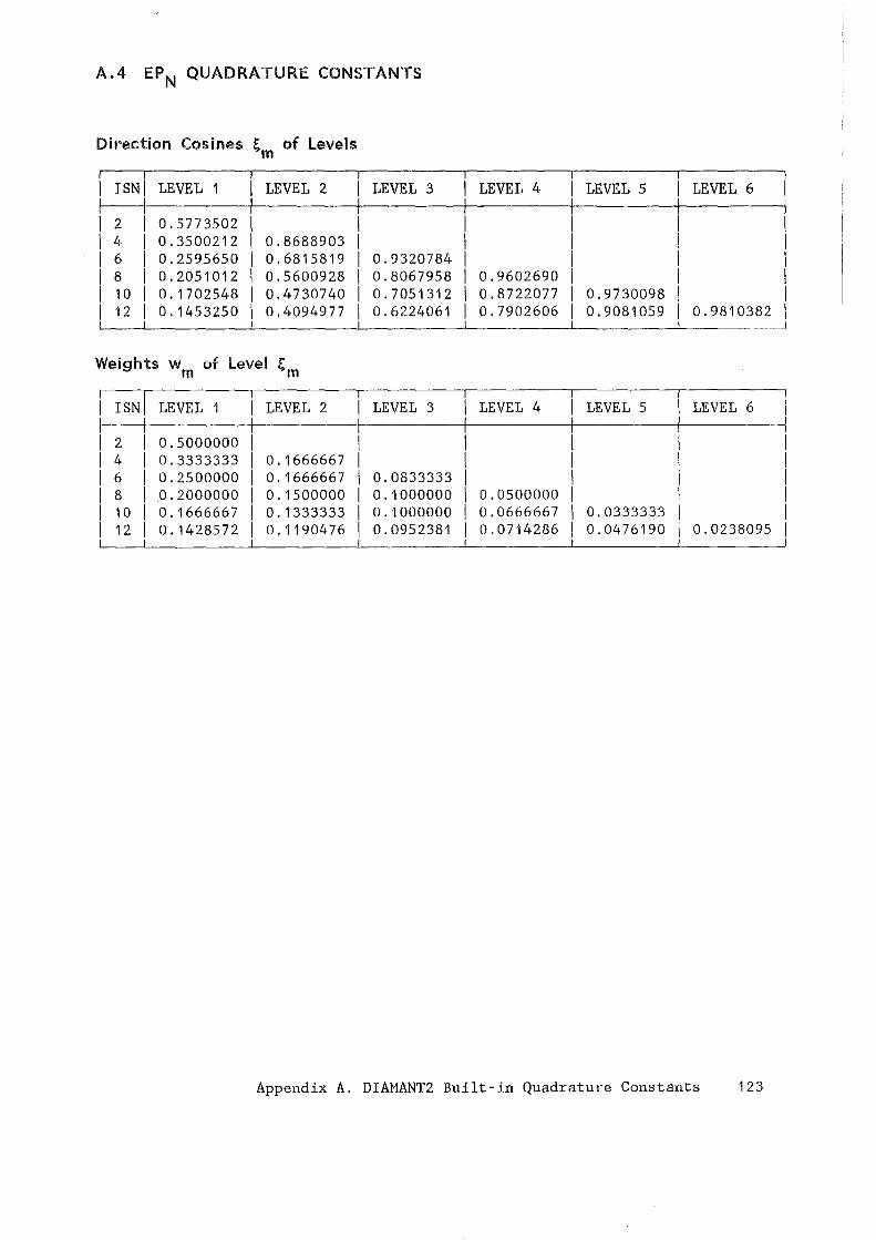
A.4 EPN QUADRATURE CONSTANTS

Direction Cosines ~m of Levels

---"! ISNI LEVEL 1 LEVEL 2 LEVEL 3 LEVEL 4 LEVEL 5 LEVEL 6 I

2 0.5773502 I 4 0.3500212 0.8688903 I 6 0.2595650 0.6815819 0.9320784 I 8 0.2051012 0.5600928 0.8067958 0.9602690 I 10 0.1702548 0.4730740 0.7051312 0. 8722077 0.9730098 I 12 0.1453250 0. 4094977 0.6224061 0.7902606 0.9081059 0.9810382 I

- _]


ISNI LEVEL 1 LEVEL 2 LEVEL 3 LEVEL 4 LEVEL 5 LEVEL 6

2 0.5000000 4 0.3333333 0.1666667 6 0.2500000 0.1666667 0.0833333 8 0.2000000 0. 1500000 0.1000000 0.0500000 10 0.1666667 0.1333333 0. 1000000 0.0666667 0.0333333 12 0.1428572 0.1190476 0.0952381 0.0714286 0.0476190 0.0238095

Appendix A. DIAMANT2 Built-in Quadrature Constants 123

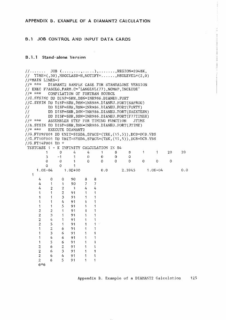
APPENDIX B. EXAMPLE OF A DIAMANT2 CALCULATION

B.l JOB CONTROL AND INPUT DATA CARDS

B. 1.1 Stand-alone Version

I I....... JOB ( .... ' ... ' ...... ) ' ....... ,REGION=2048K, II TIHE=(,30),NSGCLASS=H,NOTIFY= ...... ,HSGLEVEL=(2,0) / /~'•HAIN LINES=7 / ;~·· •'d;;'( DIAMANT2 SAMPLE GASE FOR STANDALONE VERSION II EXEC F7ASCLG,PARM.C='LANGLVL(77),NOMAP,INCLUDE 1

/ /•'• .,...,'(.,'( Cm!PILATION OF FORTRAN SOURCE //C.SYSINC DD DISP=SHR,DSN=INR986.DIANEU.FORT //C.SYSIN DD DISP=SHR,DSN=INR986.DIANEU.FORT(SAPROG) II DD DISP=SHR,DSN=INR986.DIANEU.FORT(FORTY) II DD DISP=SHR,DSN=INR986.DIANEU.FORT(SAEXTERN) II DD DISP=SHR,DSN=INR986.DIANEU.FORT(F77THIER) / /"' •'(•'••'• ASSEMBLER STEP FOR TIMING FUNCTION JTIME //A.SYSIN DD DISP=SHR,DSN=INR986.DIANEU.FORT(JTIME) / /•'• Mo'( EXECUTE DIAHANT2 //G.FT09F001 DD UNIT=SYSDA,SPACE=(TRK,(15,5)),DCB=DCB.VBS //G.FT10F001 DD UNIT=SYSDA,SPACE=(TRK,(15,5)),DCB=DCB.VBS //G.FT14F001 DD * TESTGASE 1 - K INFINITY CALCULATION IN S4

1 0 4 4 1 8 8 3 -1 0 0 0 0 0 0 0 0 0 0 0 0 0 0

1. OE-04 1. OE+OO 0.0 2.3945 1 .OE-04

4 0 0 90 8 8 4 1 1 90 7 7 4 2 2 1 4 4 1 1 2 91 1 1 1 1 3 91 1 1 1 1 4 91 1 1 1 1 5 91 1 1 2 2 1 91 1 1 2 3 1 91 1 1 2 4 1 91 1 1 2 5 1 91 1 1 1 2 6 91 1 1 1 3 6 91 1 1 1 4 6 91 1 'I 1 5 6 91 1 1 2 6 2 91 1 1 2 6 3 91 1 2 6 4 91 1 2 6 5 91 1 6•'<'6

20 20

0

0.0

Appendix B. Example of a DIANANT2 Calculation 125

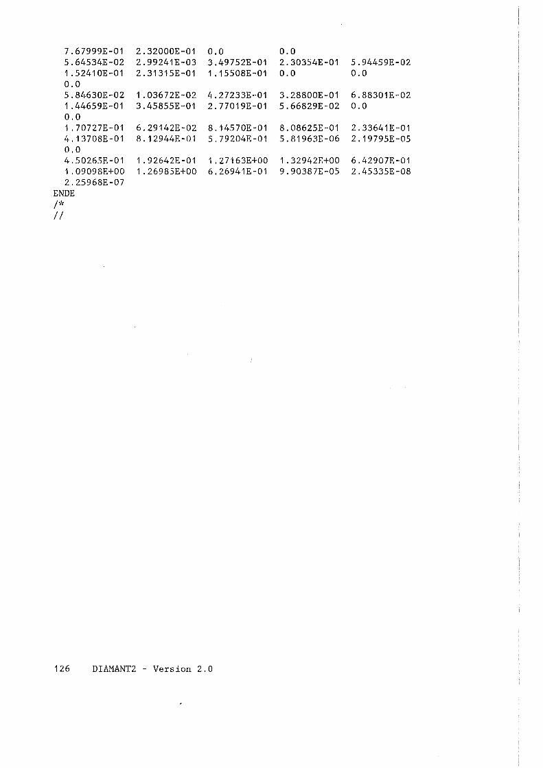
7.67999E-01 2.32000E-01 0.0 0.0 5.64534E-02 2.99241E-03 3.49752E-01 2.30354E-01 5.94459E-02 1.52410E-01 2.31315E-01 1.15508E-01 0.0 0.0 0.0 5.84630E-02 1.03672E-02 4.27233E-01 3.28800E-01 6.88301E-02 1. 44659E-01 3.45855E-01 2. 77019E-01 5.66829E-02 0.0 0.0 1 .70727E-01 6.29142E-02 8.14570E-01 8.08625E-01 2.33641E-01 4.13708E-01 8.12944E-01 5.79204E-01 5.81963E-06 2 .19795E-05 0.0 4.50265E-01 1 .92642E-01 1 .27163E+OO 1.32942E+OO 6.42907E-01 1 .09098E+OO 1 .26985E+OO 6.26941E-01 9.90387E-05 2.45335E-08 2.25968E-07

ENDE ~~~

II


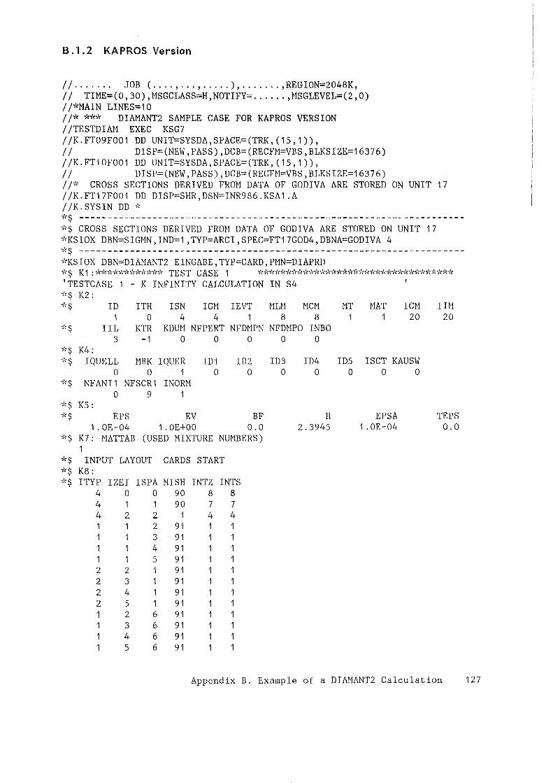
B. 1. 2 KAPROS Version

I I....... JOB ( .... ' ... ' ..... ), ....... ,REGION=2048K, I I TIME=(O, 30), MSGCLASS=H, NOTIFY= ...... ,~1SGLEVEL=(2, 0) I I'>':HAIN LINES=1 0 I 1?': ?'n'nt: DIAMANT2 SAHPLE CASE FOR KAPROS VERSION I ITESTDIMI EXEC KSG7 IIK.FT09F001 DD UNIT=SYSDA,SPACE=(TRK,(15,1)), II DISP=(NEW,PASS),DCB=(RECFN=VBS,BLKSIZE=16376) I/K.FT10F001 DD UNIT=SYSDA,SPACE=(TRK,(15,1)), II DISP=(NEW,PASS),DCB=(RECFN=VBS,BLKSIZE=16376) I 1~': CROSS SECTIONS DERIVED FRmi DATA OF GODIVA ARE STORED ON UNIT 17 IIK.FT17F001 DD DISP=SHR,DSN=INR986.KSA1 .A I IK. SYSIN DD ~·:

*$ ---------------------------------------------------------------------~"$ CROSS SECTIONS DERIVED FROH DATA OF GODIVA ARE STORED ON UNIT 17 *KSIOX DBN=SIGHN,IND=1 ,TYP=ARCI,SPEC=FT17GOD4,DBNA=GODIVA 4 *$ ---------------------------------------------------------------------?'(KSIOX DBN=DIM1ANT2 EINGABE, TYP=CARD, PNN=DIAPRD *$ K1 :************ TEST GASE 1 *********************************** 'TESTCASE 1 - K INFINITY CALCULATION IN S4 ~'($ K2: ~·( $ ID

1 ITH ISN

0 4 IGN IEVT MUI

4 1 8 MCM

8 IIL KTR KDUN NFPERT NFDNPN NFDHPO INBO

3 -1 0 0 0 0 ~·($ K4: *$ !QUELL HBK IQUER ID1 ID2 ID3

0 0 1 0 0 0 ~·($ NFANI1 NFSCR1 INORH

0 9 1 ~·($ K5: ~·($ EPS EV BF

1. OE-04 ~'($ K7: HATTAB

1

1 .OE+OO 0.0 (USED MIXTURE NUMBERS)

~·($ INPUT LAYOUT CARDS START '>'($ K8: ~'($ ITYP

4 4 4 1 1

2 2 2 2 1 1 1

IZEI ISPA HISH INTZ INTS 0 0 90 8 8 1 1 90 7 7 2 2 1 4 4 1 2 91 1 1 3 91 1 1 4 91 1 1 5 91 1 2 1 91 1 3 1 91 4 1 91 5 1 91 2 6 91 3 6 91 4 6 91 5 6 91

0

ID4 0

H 2.3945

MT 1

IDS 0

~1AT IC~I

20

ISCT KAUSW 0

EPSA 1 .OE-04

0

IU! 20

TEPS 0.0

Appendix B. Example of a DIAHANT2 Calculation 127

2 6 2 91 1 2 6 3 91 1 2 6 4 91 1 2 6 5 91 1

~'~'$ LAYOUT END 61~6

;'l'$ CROSS SECTION INPUT IS DONE BY SIGMN BLOCK 'ENDE' ;'($;"'$ *$ ---------------------------------------------------------------------;"'KSIOX DBN=INIThREADtsDIAHAN, TYP=CARD, P~1N=PRDUM 09 'SCRATCH15UNIT1511515' 1 6 0 1 10 'SCRATCH15UNIT152tsts' 1 6 0 1 14 'DIAHANT215EINGABE' 1 1 0 0

*$ ---------------------------------------------------------------------;'~80 SM=DIANEU

II


P> '"d '"d (tl l:::l p..

""'" ~

tx:1

l:%:1 :>< ·~

a '"d I-' (tl

0 H1

~

t::l H P> ::s:: ~ ~ N

0 0> I-' (")

~ I-' 0> rt

""'· 0 l:::l

N \.D

**** * *** * * *** * * ***** ** * * * * * ** ** * * ** * * * * * * * ***** * * * ***** * * * * * * * * * * * * * * * ** * * **** * * * * * * * * * * ****

**** ***** *** **** ***** * * * * * * *

*** * ***** **** * * * * * * * *

**** * * * * * *

************************* * * * * * * * *

* * * * * * * * * * * * * * * *

********************************* * * * * * * * * * *

* * * * * * * * * * * * * * * * * * * *

***************************************** * * * * * * * * * *

* * * * * * * * * * * * * * * * * * * *

********************************* * * * * * * * *

* * * * * * * * * * * * * * * *

************************* * * * * * *

* * * * * * * * * * * *

***************** * * * * * * * *

* * * * *********

THIS ISA MAJOR REVISION OF THE DIAMANT2 CODE (VERSION 1.4) - NEW RELEASE: 2.0 THIS VERSION IS PROGRAMMED ACCORDING TO THE FORTRAN77 STANDARDS A GREAT DEAL OF EFFORT HAS GONE INTO CODE RESTRUCTURING, CLARIFICATION AND DOCUMENTATION THIS VERSION SHOULD RUN EFFICIENTLY ON VECTOR COMPUTERS, TOO

OJ

N

0 c -1 ." c -1 r (/')

-1 0 -n -1 :I: !Tl

(/')

):> s:: ." r !Tl

." :;101 0 OJ rITI s::

U)

0

t::;j H

> 3: > ~ N

<: CD 1-i [/J

f-'· 0 :::1

N

0

***************************************************************** * * * EINHEIT 9 REALISIERT ALS EXTERNE EINHEIT * *EINHEIT 10 REALISIERT ALS EXTERNE EINHEIT * *EINHEIT 14 REALISIERT ALS NORMALER DB: DIAMANT2 EINGABE 1 * * * *****************************************************************

FREE MAIN STORAGE PLAGE IN THE BEGINNING 214430 WORDS

VALUES OF THE PARAMETER STATEMENT USED TO CREATE LOAD MODULE ============================================================

IGMMAX 26 IGPMAX 27 IREGMX 30 ISNMAX 12 ISCTMX 6

JMMMAX 138 LPMAX 65535 MINVEC 6 MATMAX 89 MAXFI L 40 MTVP 90 MTRP 91 MTJP 92 NACMAX 1 NWMAX 1 NCMAX 2 LENCOM 1 NIVMAX 21

EPSCPU l.OOOOE-20 EPSMIN l.OOOOE-06 PI 3.1416E+OO PIHALF 1.5708E+OO PISIXT 5.2360E-01

LREBAL TRUE LTRANS TRUE LXSCHK TRUE

MAXIMUM NUMBER OF ENERGY GROUPS IGMMAX + 1 MAXIMUM NUMBER OF DISJOINT MIXTURE REGIONS MAXIMUM ORDER OF THE ANGULAR DISCRETIZATION MAXIMUM ORDER OF ANISOTRPIC SCATTERING JMMMAX=ISNMAX+ISNMAX*( ISNMAX+2)*3/4 MAXIMUM LENGTH OF A SINGLE DO-LOOP (SIGNIFICANT ONLY FOR CYBER 205) MINIMUM LENGTH OF A DO-LOOP TO BE EXECUTED IN VECTOR MODE MAXIMUM NUMBER OF XS-TABLES MAXIMUM VALUE FOR FORTRAN UNIT NUMBERS MIXTURENUMBER TO REPRESENT VACUUM BOUNDARY'CONDITION IN INPUT ( = MATMAX + 1) MIXTURE NUMBER TO REPRESENT REFLECTIVE BOUNDARY CONDITION IN INPUT ( = MATMAX + 2) MIXTURE NUMBER TO REPRESENT BOUNDARY FLUX CONDITION IN INPUT ( = MATMAX + 3) NUMBER OF WORDS RESERVED FOR REAL STORAGE NUMBER OF WORDS RESERVED FOR INTEGER STORAGE TOTAL NUMBER OF WORDS OF RESERVED STORAGE ( NCMAX = NACMAX + NWMAX ) LENGTH OF WORKING ARRAY IN COMMON BLOCK /COMMOM/ NIVMAX=ISNMAX*( ISNMAX+2)/8

ALL REAL VALUES BELOW THIS THRESHOLD ARE CONSIDERED TO BE ZERO MINIMUM VALUE FOR CONVERGENCE CRITERIA (DEPENDS ON MACHINE PRECISION) VALUE OF THE CONSTANT PI Pl/2. Pl/6.

INNER ITERATION ACCELERATION PERFORM P1 GORREGTION IN XS-TABLE REPLACE INPUT ABSORPTION XS BY CALCULATED XS

CPU TIME OVERHEAD IN EACH CALL TO FUNCTION TASKTI : 0.0 SECONDS

0> '0 '0

CD ~ 0.. 1-'· >: b:l

t:r:l >: ll> 3 '0 .....

CD

0 1-h

ll>

t:J H 0> ;:;;: 0> z ~ N

0 ll> ..... (")

~ ..... ll> rt 1-'· 0 ~

UJ

TITLE OF THIS RUN:

********************************************************************** * * TESTGASE 1 - K INFINITY CALCULATION IN 54 *

* * * **********************************************************************

NO FLUX GUESS

POINTER DATABLOCK WITH 1054 WORDS OF 4 BYTES EACH CREATED; VALUE OF POINTER IS:

DISTRIBUTION OF WORKING ARRAY lW ================================

ARRAY MODBND MIXDIS I HLP1 MIXREG MODEL MODANI IHLP2 START IN lW 3144 3684 3812 3940 4068 4196 4197 LENGTH 540 128 128 128 128 1 1

START OF WORKING ARRAY AT lW( 3144), END OF WORKING ARRAY AT lW( 4198)

POINTER DATABLOCK WITH 6612 WORDS OF 4 BYTES EACH CREATED; VALUE OF POINTER IS:

DISTRIBUTION OF WORKING ARRAY A ================================

ARRAY XNA XNB XNC HLP1 HLP2 XNBI XNBO XNAI START IN A 4199 4207 4215 4223 4231 4239 4415 5119 LENGTH 8 8 8 8 8 176 704 176

ARRAY XNCO FLXANG FLXNEW s FLXOLD c XTOT XSSCAT START IN A 6175 6879 7007 7135 7263 7391 7523 7535 LENGTH 704 128 128 128 128 132 12 128

ARRAY FG FGOLD BUCK EXTSOU XAIJ XBIJ XCIJ BI L 1 START IN A 7803 7931 8059 8060 8061 8765 9469 10173 LENGTH 128 128 1 1 704 704 704 120

ARRAY FLXSKA ss T TW TF TFOLD XSANI START IN A 10293 10805 10806 10807 10808 10809 10810 LENGTH 512 1 1 1 1 1 1

START OF WORKING ARRAY AT A( 4199), END OF WORKING ARRAY AT A( 10811 )

REAL MAIN STORAGE 6612 INTEGER MAIN STORAGE 1054 NUMBER OF AUXILIARY DATASETS USED 0

3144

4199

XNAO XNCI 5295 5999

704 176

XSFI SS GRPSOU 7663 7675

12 128

BI L2 BI L3 10293 10293

1 1

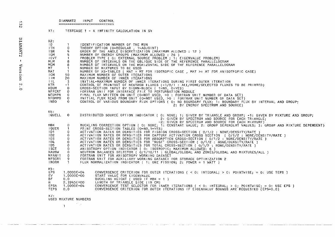
w N

t:l H

> ::;:: > ~ N

<: (1) t1 [I)

f-'· 0 ::s N

0

DIAMANT2 INPUT CONTROL ==========================

K1:

K2: ID ITH ISN IGM IEVT

MLM MCM MT MAT ICM IIM II L KTR KDUM NFPERT NFDMPN NFDMPO INBO

K4: I QUELL

MBK !QUER I D1 ID2 ID3 ID4 ID5 ISCT KAUSW NFANI1 NFSCR1 I NORM

K5: EPS EV BF H EPSA TEPS

K7:

TESTGASE 1 - K INFINITY CALCULATION IN S4

1 0 4 4 1 8 8 1 1

50 20

3 -1

0 0 0 0 0

0

0 1 0 0 0 0 0 0 0 0 9 1

IDENTIFICATION NUMBER OF THE RUN THEORY OPTION (O=REGULAR , 1=ADJOINT) ORDER OF THE ANGLE DISCRETIZATION (MAXIMUM ALLOWED : 12 ) NUMBER OF ENERGY GROUPS (MAXIMUM ALLOWED : 26 ) PROBLEM TYPE ( 0: EXTERNAL SOURCE PROBLEM; 1: EIGENVALUE PROBLEM) NUMBER OF INTERVALS ON THE OBLIQUE SIDE OF THE REFERENCE PARALLELOGRAM NUMBER OF INTERVALS ON THE HORIZONTAL SIDE OF THE REFERENCE PARALLELOGRA~I NUMBER OF MIXTURES TO BE USED NUMBER OF XS-TABLES ( MAT = MT FOR ISOTROPIC GASE , MAT >= MT FOR ANISOTROPIC GASE) MAXIMUM NUMBER OF OUTER ITERATIONS MAXIMUM NUMBER OF INNER ITERATIONS INITIAL-MAXIMUM NUMBER OF INNER ITERATIONS DURING FIRST OUTER ITERATION CONTROL OF PRINTOUT OF NEUTRON FLUXES (-1/0/1 : ALL/NONE/SELEGTED FLUXES TO BE PRINTED) CROSS-SECTION INPUT BY SIGMN-BLOCK ( 1=NO, O=YES) FORTRAN UNIT FOR INTERFACE FILE TO PERTURBATION MODULE FINAL FLUX WRITTEN ON UNIT (O=NOT USED, >0 : FORTRAN UNIT NUMBER OF DATA SET) INITIAL FLUX READ FROM UNIT (O=NOT USED, >0 : FORTRAN UNIT NUMBER OF DATA SET) CONTROL OF VARIOUS BOUNDARY FLUX OPTIONS ( 0: NO BOUNDARY FLUX; 1: BOUNDARY FLUX BY INTERVALAND GROUP;

2: BY ENERGY SPECTRUM AND SOURCE)

DISTRIBUTED SOURCE OPTION INDICATOR ( 0 NONE; 1: GIVEN BY TRIANGLE AND GROUP; -1: GIVEN BY MIXTURE AND GROUP; 2 GIVEN BY SPECTRUM AND SOURCE FOR EACH TRIANGLE;

-2 GIVEN BY SPEGTRUM AND SOURCE FOR EACH MIXTURE) BUGKLING GORREGTION OPTION ( 0: NONE; 1 GONSTANT VALUE; 2: GROUP DEPENDENT VALUES; 3: GROUP AND MIXTURE DEPENDENT) PRINT GROSS-SEGTION TABLES (O=N0,1=YES) AGTIVATION RATES OR DENSITIES FOR FISSION GROSS-SEGTION ( 0/1/2 : NONE/DENSITY/RATE ) AGTIVATION RATES OR DENSITIES FOR CAPTURE AGTIVATION CROSS SECTION ( 0/1/2 : NONE/DENSITY/RATE AGTIVATION RATES OR DENSITIES FOR ABSORPTION GROSS-SECTION ( 0/1/2 : NONE/DENSITY/RATE ) AGTIVATION RATES OR DENSITIES FOR 'NUSF' CROSS-SECTION ( 0/1/2 : NONE/DENSITY/RATE ) AGTIVATION RATES OR DENSITIES FOR TOTAL GROSS-SECTION ( 0/1/2 : NONE/DENS!TY/RATE ) ANISOTROPY OPTION INDICATOR ( 0: ISOTROPIC; MAXIMUM ALLOWED: 6 ) NEUTRON BALANGES SELECTOR ( 0/1/10/11 : GLOBAL/GLOBAL AND ZONES/GLOBAL AND MIXTURES/ALL FORTRAN UNIT FOR ANISOTROPY WORKING DATASET FORTRAN UNIT FOR AUXILIARY WORKING DATASET FOR STORAGE OPTIMIZATION 2 FLUX NORMALIZATION INDIGATOR ( 1: ONE FISSION; 2: POWER= 1 WATT )

1. OOOOE-04 1.0000E+OO 0.0 2.3945E+OO 1. OOOOE-04 0.0

CONVERGENCE GRITERION FOR OUTER ITERATIONS ( < 0: INTEGRAL; > 0: POINTWISE; = 0: USE TEPS ) START VALUE FOR EIGENVALUE BUGKLING HEIGHT ( USED IF MBK = 1 ) LENGTH OF TRIANGLE SIDE (IN CM) CONVERGENGE TEST SELEGTOR FOR INNER ITERATIONS ( < 0: INTEGRAL; > 0; POINTWISE; = 0: USE EPS ) GONVERGENGE CRITERION FOR OUTER ITERATIONS IF EIGENVALUE BOUNDS ARE REQUESTED (EPS=O.O)

USED MIXTURE NUMBERS

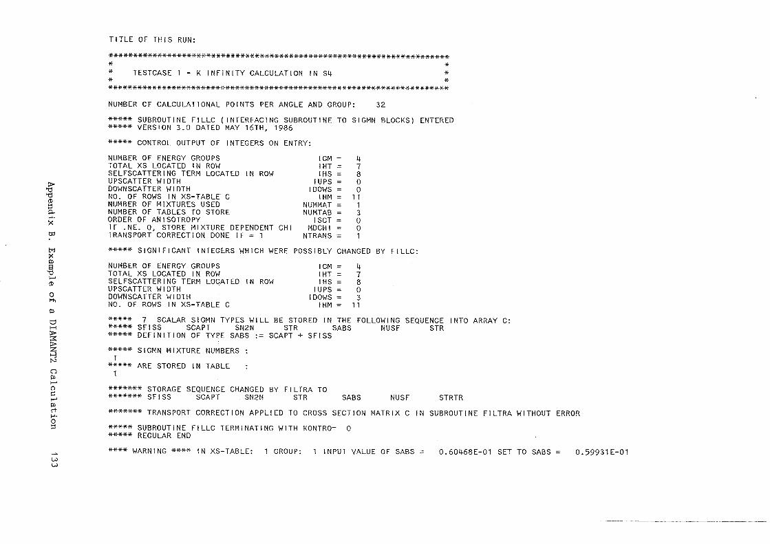
~ '"Cl (I)

::l p.. f-'· X

t::J:j

t?=J X !)) 3

'"Cl ..... (I)

0 t-h

!))

t::J 1-1

~ ~ N

0 !)) ..... (")

>::! t-' !)) rt f-'· 0 ::l

VJ VJ

TITLE OF THIS RUN:

********************************************************************** * * *

TESTGASE 1 - K INFINITY CALGULATION IN S4 * * * **********************************************************************

NUMBER OF CALGULATIONAL POINTS PER ANGLE AND GROUP: 32

***** SUBROUTINE FILLC ( INTERFAG!NG SUBROUTINE TO SIGMN BLOCKS) ENTERED ***** VERSION 3.0 DATED MAY 16TH, 1986

***** CONTROL OUTPUT OF INTEGERS ON ENTRY:

NUMBER OF ENERGY GROUPS TOTAL XS LOGATED IN ROW SELFSGATTERING TERM LOCATED IN ROW UPSGATTER WIDTH DOWNSGATTER WIDTH NO. OF ROWS IN XS-TABLE C NUMBER OF MIXTURES USED NUMBER OF TABLES TO STORE ORDER OF ANISOTROPY IF .NE. 0, STORE MIXTURE DEPENDENT CHI TRANSPORT GORREGTION DONE IF = 1

IGM IHT IHS

I UPS IDOWS

IHM NUMMAT NUMTAB

ISGT MDCHI

NTRANS

4 7 8 0 0

11 1 3 0 0 1

***** SIGNIFICANT INTEGERS WHICH WERE POSSIBLY CHANGED BY FILLC:

NUMBER OF ENERGY GROUPS TOTAL XS LOCATED IN ROW SELFSGATTERING TERM LOCATED IN ROW UPSGATTER WIDTH DOWNSGATTER WIDTH NO. OF ROWS IN XS-TABLE G

IGM IHT IHS

I UPS IDOWS

IHM

4 7 8 0 3

11

***** 7 SGALAR SIGMN TYPES WILL BE STORED IN THE FOLLOWING SEQUENCE INTO ARRAY C: ***** SFISS SGAPT SN2N STR SABS NUSF STR ***** DEFINITION OF TYPE SABS := SCAPT + SFISS

***** SIGMN MIXTURE NUMBERS 1

*****ARE STORED IN TABLE

*******STORAGE SEQUENCE GHANGED BY FILTRA TO ******* SFISS SCAPT SN2N STR SABS NUSF STRTR

*******TRANSPORT GORREGTION APPLIED TO CROSS SECTION MATRIX G IN SUBROUTINE FILTRA WITHOUT ERROR

***** SUBROUTINE FILLC TERMINATING WITH KONTRO= 0 ***** REGULAR END

**** WARNING **** IN XS-TABLE: 1 GROUP: 1 INPUT VALUE OF SABS 0.60468E-01 SET TO SABS 0.59931E-01

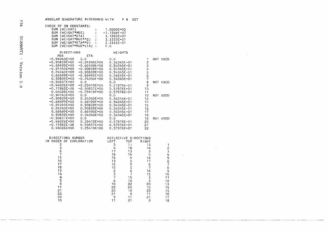
ANGULAR QUADRATURE PERFORMED WITH P N SET w +:- CHECK OF SN CONSTANTS:

SUM (WEIGHT) : 1. OOOOE+OO SUM (WEIGHT*MUE) : -1. 1548E-07

t;j SUM (WEIGHT*ETA) : 3.1292E-07 H SUM (WEIGHT*MUE**2) : 3.3333E-01 P> SUM (WEIGHT*ETA**2) : 3.3333E-01 ::s:: SUM (WEIGHT*MUE*ETA) : 0.0 P> z t-3 DIRECTIONS WEIGHTS N MUE ETA

-0.94043E+OO 0.0 0.0 1 NOT USED < -0.90839E+OO -0.24340E+OO 0.54345E-01 2 CO -0.66499E+OO -0.66499E+OO 0.54345E-01 3 f"i -0.24340E+OO -0.90839E+OO 0.54345E-01 4 (IJ

0.24340E+OO -0.90839E+OO 0.54345E-01 5 1-'· 0 0.66499E+OO -0.66499E+OO 0.54345E-01 6 ~ 0.90839E+OO -0.24340E+OO 0.54345E-01 7 N -0.50837E+OO 0.0 0.0 8 NOT USED 0 -0.44026E+OO -0.25419E+OO 0.57976E-01 9

-0.15962E-06 -0.50837E+OO 0.57976E-01 10 0.44026E+OO -0.25419E+OO 0.57976E-01 11

-0.94043E+OO 0.0 0.0 12 NOT USED -0.90839E+OO 0.24340E+OO 0.54345E-Ol 13 -0.66499E+OO 0.66499E+OO 0.54345E-01 14 -0.24340E+OO 0.90839E+OO 0.54345E-01 15

0.24340E+OO 0.90839E+OO 0.54345E-01 16 0.66499E+OO 0.66499E+OO 0.54345E-01 17 0.90839E+OO 0.24340E+OO 0.54345E-01 18

-0.50837E+OO 0.0 0.0 19 NOT USED -0.44026E+OO 0.25419E+OO 0.57976E-01 20 -0.15962E-06 0.50837E+OO 0.57976E-01 21

0.44026E+OO 0.25419E+OO 0.57976E-01 22

DIRECTIONS NUMBER REFLECTIVE DIRECTIONS IN ORDER OF EXPLORATION LEFT TOP RIGHT

2 5 17 13 1 3 4 18 14 2 6 17 13 5 3 7 18 14 4 4

15 14 4 18 5 16 13 5 17 6 17 16 2 6 7 18 15 3 7 8 13 2 6 16 9 14 3 7 15 10

4 7 15 3 11 5 6 16 2 12 9 10 22 20 13

11 22 20 10 14 21 20 10 22 15 22 21 9 11 16 20 9 11 21 17 10 11 21 9 18

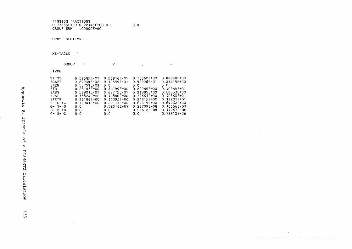
> "0 "0 (l)

~ p. f-'· ~

tp

~ ~ Pl 3 "0 ....... (l)

0 H'l

Pl

t:::l H

> 3: > z >-3 N

Cl Pl ....... (')

c ....... Pl rt f-'· 0 ~

(.;.)

\J1

FISSION FRAGTIONS 0.77655E+OO 0.22345E+OO 0.0 GROUP SUM= l.OOOOOE+OO

CROSS SECTIONS

XS-TABLE

TYPE

SFI SS SCAPT SN2N STR SABS NUSF STRTR

GROUP

S G->G G- 1->G G- 2->G G- 3->G

0.57545E-01 0.29234E-02 0.53731E-03 0.23103E+OO 0.59931E-01 0.15524E+OO o.23188E+oo 0.11941E+OO 0.0 0.0 0.0

2

0.58916E-01 0. 10859E-01 0.0 0.34149E+OO 0.69175E-01 0. 14580E+OO 0.36095E+OO 0.29115E+OO 0.52518E-01 0.0 0.0

0.0

3 4

0.16362E+OO 0.44838E+OO 0.56226E-01 0.23215[+00 0.0 0.0 0.89260E+OO 0. 10564E+01 0.21985E+OO 0.68053E+OO 0.39661E+OO 0. 10863E+01 0.91315E+OO 0.13231E+01 0.69319[+00 0.64262E+OO 0.23709E-04 0. 10566E-03 0.21618E-04 0.17267E-06 0.0 0.72812E-06

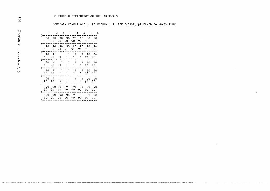
VJ 0\

t::1 H p::.

§; z >-,3 N

<: (D 1-j Cll f-'-0 ::l

N

0

MIXTURE DISTRIBUTION ON THE INTERVALS

BOUNDARY CONDITIONS 90=VACUUM, 91=REFLECTIVE, 92=FIXED BOUNDARY FLUX

1 2 3 4 5 6 7 8 o--------------------------------

90 90 90 90 90 90 90 90 90 90 90 90 90 90 90 90

1--------------------------------90 90 90 90 90 90 90 90

90 90 91 91 91 91 90 90 2--------------------------------

90 91 1 1 1 1 90 90 90 90 1 1 1 1 91 90

3--------------------------------90 91 1 1 1 1 90 90

90 90 1 1 1 1 91 90 4--------------------------------

90 91 1 1 1 1 90 90 90 90 1 1 1 1 91 90

5--------------------------------90 91 1 1 1 1 90 90

90 90 1 1 1 1 91 90 6--------------------------------

90 90 91 91 91 91 90 90 90 90 90 90 90 90 90 90

7--------------------------------90 90 90 90 90 90 90 90

90 90 90 90 90 90 90 90 8--------------------------------

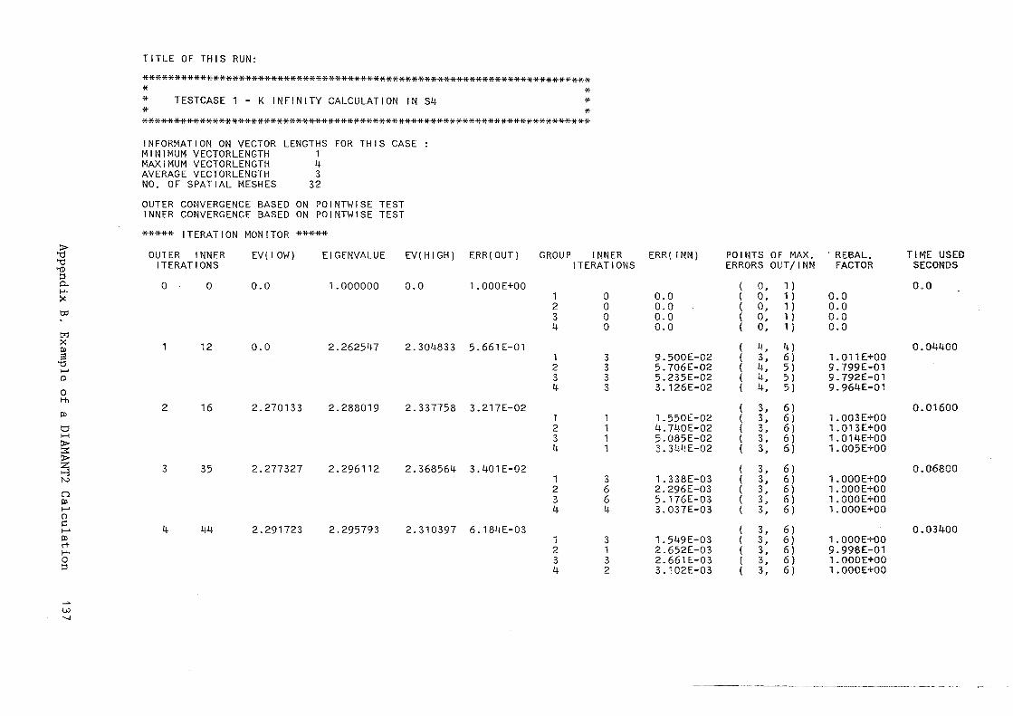
:> '1j '1j >(!)

~ p.. f-'· >: t:P

t:"l >: Cl 3

'1j ....... (!)

0 t-h

Cl

t:::! H :> :::::: :> z >-3 N

0 !ll ....... ()

c ....... !ll rt f-'· 0 ~

VJ ......

TITLE OF THIS RUN:

********************************************************************** * * * TESTGASE 1 - K INFINITY CALCULATION IN S4 * * * **********************************************************************

INFORMATION ON VECTOR LENGTHS FORTHIS CASE : MINIMUM VECTORLENGTH 1 MAXIMUM VECTORLENGTH 4 AVERAGE VECTORLENGTH 3 NO. OF SPATIAL MESHES 32

OUTER CONVERGENCE BASED ON POINTWISE TEST INNER CONVERGENCE BASED ON POINTWISE TEST

***** ITERATION MONITOR *****

OUT ER INNER EV(LOW) EIGENVALUE EV(HIGH) ERR(OUT) GROUP INNER ITERATIONS ITERATIONS

0 0 0.0 1.000000 0.0 1. OOOE+OO 1 0 2 0 3 0 4 0

1 12 0.0 2.262547 2.304833 5.661E-01 1 3 2 3 3 3 4 3

2 16 2.270133 2.288019 2.337758 3.217E-02 1 1 2 1 3 1 4 1

3 35 2.277327 2.296112 2.368564 3.401E-02 1 3 2 6 3 6 4 4

4 44 2.291723 2.295793 2.310397 6.184E-03 1 3 2 1 3 3 4 2

ERR( INN) POINTS OF MAX. ERRORS OUT/INN

( 0, 1 ) 0.0 ( 0, 1 ) 0.0 ( 0, 1 ) o.o ( 0, 1 l 0.0 ( 0, 1 )

( 4, 4) 9.500E-02 ( 3, 6) 5.706E-02 ( 4, 5) 5.235E-02 ( 4, 5) 3.126E-02 ( 4, 5)

( 3, 6) 1.550E-02 ( 3, 6) 4.740E-02 ( 3, 6) 5.085E-02 ( 3, 6) 3.344E-02 ( 3, 6)

( 3, 6) 1.338E-03 ( 3, 6) 2.296E-03 ( 3, 6) 5.176E-03 ( 3, 6) 3. 037E-03 ( 3, 6)

( 3, 6) 1. 549E-03 ( 3, 6) 2.652E-03 ( 3, 6) 2.661E-03 ( 3, 6) 3. 1 02E-03 ( 3, 6)

' REBAL. FACTOR

0.0 0.0 0.0 0.0

1.011E+OO 9.799E-01 9.792E-01 9.964E-01

1. 003 E+OO 1. 013E+OO 1.014E+OO 1.005E+OO

l.OOOE+OO 1. OOOE+OO 1.000E+OO 1. OOOE+OO

l.OOOE+OO 9.998E-01 l.OOOE+OO 1 .OOOE+OO

TIME USED SECONDS

0.0

0.04400

0.01600

0.06800

0.03400

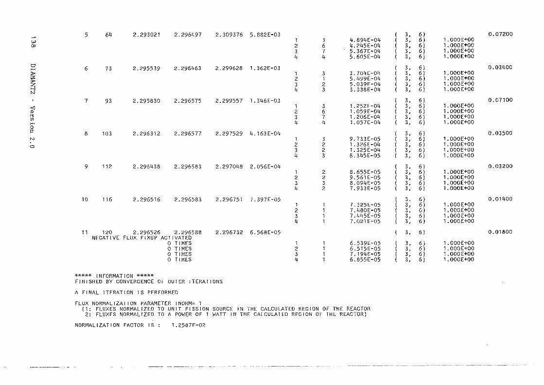
5 64 2.293021 2.296497 2.309376 5.882E-03 ( 3, 6) 0.07200 UJ 1 3 4.894E-04 ( 3, 6) l.OOOE+OO ():) 2 6 4.245E-04 ( 3, 6) l.OOOE+OO

3 7 5.367E-04 ( 3, 6} l.OOOE+OO 4 4 5.605E-04 ( 3, 6) 1.000E+OO

t:::J 6 73 2.295539 2.296463 2.299628 1.362E-03 ( 3, 6) 0.03400 H D> 1 3 3.704E-04 ( 3, 6) 1 .OOOE+OO :::::: 2 1 5.499E-04 ( 3, 6) 1 .OOOE+OO D> z 3 2 5.039E-04 ( 3, 6) 1. OOOE+OO >-:3 4 3 3.338E-04 ( 3, 6} l.OOOE+OO N

7 93 2.295830 2.296575 2.299557 1. 346E-03 ( 3, 6) 0.07100 <:: 1 3 1.252E-04 ( 3, 6) 1 .OOOE+OO (!) 2 6 1.059E-04 ( 3, 6) 1. OOOE+OO 1-1 3 7 1 . 206E-04 ( 3, 6) l.OOOE+OO [11

f-'· 4 4 1.057E-04 ( 3, 6) 1.000E+OO 0 ::l 8 103 2.296312 2.296577 2.297529 4.163E-04 ( 3, 6) 0.03500 N 1 3 9.733E-05 ( 3, 6) 1. OOOE+OO 0 2 2 1.326E-04 ( 3, 6) l.OOOE+OO

3 2 1.325E-04 ( 3, 6) 1.000E+OO 4 3 8.345E-05 ( 3, 6) 1.000E+OO

9 112 2.296438 2.296583 2.297048 2.056E-04 ( 3, 6) 0.03200 1 2 8.655E-05 ( 3, 6) 1.000E+OO 2 2 9.561E-05 ( 3, 6) 1. OOOE+OO 3 3 8.094E-05 ( 3, 6) 1. OOOE+OO 4 2 7.933E-05 ( 3, 6) 1. OOOE+OO

10 116 2.296516 2.296583 2.296751 7.397E-05 ( 3, 6) 0.01400 1 1 7.325E-05 ( 3, 6) 1. OOOE+OO 2 1 7.480E-05 ( 3, 6) 1.000[+00 3 1 7.445E-05 ( ':t 6) l.OOOE+OO ~,

4 1 7.021E-05 ( 3, 6) l.OOOE+OO

11 120 2.296526 2.296588 2.296732 6.568E-05 ( 3, 6) 0.01800 NEGATIVE FLUX FiXUP ACTIVATED

0 TIMES 1 1 6.539E-05 ( 3, 6) l.OOOE+OO 0 TIMES 2 1 6.515E-05 ( 3, 6) 1. OOOE+OO 0 TIMES 3 1 7. 194E-05 ( 3, 6) l.OOOE+OO 0 TIMES 4 1 6.855E-05 ( 3, 6) 1. OOOE+OO

***** INFORMATION ***** FINISHED BY CONVERGENCE OF OUTER ITERATIONS

A FINAL ITERATION IS PERFORMED

FLUX NORMALIZATION PARAMETER !NORM= 1 ( 1 : FLUXES NORMALIZED TO UNIT FISSION SOURCE IN THE CALCULATED REGION OF THE REACTOR 2: FLUXES NORMALIZED TO A POWER OF 1 WATT IN THE CALCULATED REGION OF THE REACTOR)

NORMALIZATION FACTOR IS : 1.2587E-02

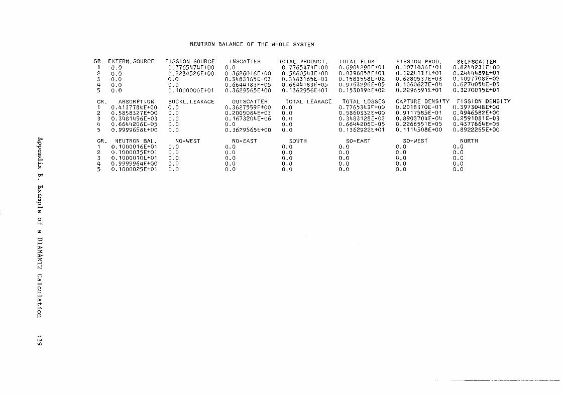
~ '0 (!)

:::l 0. f-'· X

0::1

M X ll> 3 '0 ...... (!)

0 1-T>

ll>

t:l H ll> ;::;:: ll> z >-3 N

0 ll> ...... ()

~ ...... ll> rt f-'· 0 :::l

w \.0

GR. EXTERN.SOURCE 1 0.0 2 0.0 3 0.0 4 0.0 5 0.0

GR. ABSORPTION 1 0.4137784E+OO 2 0.5858327E+OO 3 0.3481456E-03 4 0.6644206E-05 5 o.9999658E+oo

GR. NEUTRON BAL. 1 0. 1000016E+01 2 0. 1000035E+Ol 3 0. 1000010E+01 4 0.9999964E+OO 5 0. 1000025E+01

NEUTRON BALANCE OF THE WHOLE SYSTEM

FISSION SOURCE INSGATTER TOTAL PRODUCT. 0.7765474E+OO 0.0 0.7765474E+OO 0.2234526E+OO 0.3626016E+OO 0.5860543E+OO 0.0 0.3483165E-03 0.3483165E-03 0.0 0.6644183E-05 0.6644183E-05 0. 1000000E+01 o.3629565E+oo 0. 1362956E+01

BUCKL.LEAKAGE OUTSGATTER TOTAL LEAKAGE 0.0 0.3627559E+OO 0.0 0.0 0.2005084E-03 0.0 0.0 0. 1673204E-06 0.0 0.0 0.0 0.0 0.0 0.3629565E+OO 0.0

NO-WEST NO-EAST SOUTH 0.0 0.0 0.0 0.0 0.0 0.0 0.0 0.0 0.0 0.0 0.0 0.0 0.0 0.0 0.0

TOTAL FLUX FISSION PROD. SELFSCATTER 0.6904290E+01 0.1071836E+01 0.8244231E+OO 0.8396058E+01 0. 1224117E+01 0.2444489E+01 0.1583558E-02 0.6280537E-03 0. 1097708E-02 0.9763296E-05 0.1060627E-04 0.6274054E-05 0.1530194E+02 0.2296591E+01 0.3270015E+01

TOTAL LOSSES CAPTURE DENSITY FISSION DENSITY 0.7765343E+OO 0.2018370E-01 0.3973048E+OO 0.5860332E+OO 0. 9117585E-01 0.4946582E+OO 0.3483128E-03 0.8903704E-04 0.2591081E-03 0.6644206E-05 0.2266551E-05 0.4377664E-05 0.1362922E+Ol 0.1114508E+OO 0.8922265E+OO

SO-EAST SO-WEST NORTH 0.0 0.0 0.0 0.0 0.0 0.0 0.0 0.0 0.0 0.0 0.0 0.0 0.0 0.0 0.0

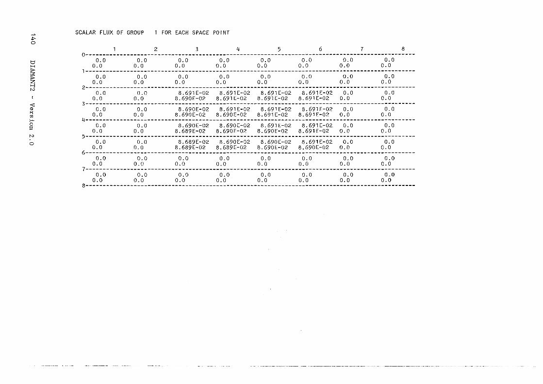
+' 0

b H

> :::;::: > z t-3 N

-<: (!) 1'1 [fJ

1-'· 0 ::l

N

0

SCALAR FLUX OF GROUP FOR EACH SPACE POINT

1 2 3 4 5 6 7 8 0------------------------------------------------------------------------------------------------o.o 0.0 0.0 0.0 0.0 0.0 0.0 0.0

0.0 0.0 0.0 0.0 0.0 0.0 0.0 0.0 1------------------------------------------------------------------------------------------------o.o 0.0 0.0 0.0 0.0 0.0 0.0 0.0

0.0 0.0 0.0 0.0 0.0 0.0 0.0 0.0 2------------------------------------------------------------------------------------------------o.o 0.0 8.691E-02 8.691E-02 8.691E-02 8.691E-02 0.0 0.0

0.0 0.0 8.690E-02 8.691E-02 8.691E-02 8.691E-02 0.0 0.0 3------------------------------------------------------------------------------------------------o.o 0.0 8.690E-02 8.691E-02 8.691E-02 8.691E-02 0.0 0.0

0.0 0.0 8.690E-02 8.690E-02 8.691E-02 8.691E-02 0.0 0.0 4--------------------------------------------------------------------------------------·----------o.o 0.0 8.690E-02 8.690E-02 8.691E-02 8.691E-02 0.0 0.0

0.0 0.0 8.689E-02 8.690E-02 8.690E-02 8.691E-02 0.0 0.0 5------------------------------------------------------------------------------------------------o.o 0.0 8.689E-02 8.690E-02 8.690E-02 8.691E-02 0.0 0.0

0.0 0.0 8.689E-02 8.689E-02 8.690E-02 8.690E-02 0.0 0.0 6------------------------------------------------------------------------------------------------o.o 0.0 0.0 0.0 0.0 0.0 0.0 0.0

0.0 0.0 0.0 0.0 0.0 0.0 0.0 o.o 7------------------------------------------------------------------------------------------------o.o 0.0 0.0 0.0 0.0 0.0 0.0 0.0

0.0 0.0 0.0 0.0 0.0 0.0 0.0 0.0 8------------------------------------------------------------------------------------------------

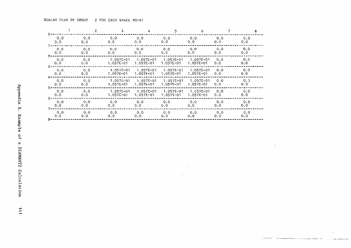
.;-"0

CD !:j 0. f-'· X

t::rl

tz:j X tll 8

"0 1-' CD

0 1-h

tll

t:l H

~ ~ N

0 tll 1-' n ;::: 1-' tll rt f-'· 0 !:j

~

SCALAR FLUX OF GROUP 2 FOR EACH SPACE POINT

1 2 3 4 5 6 7 8 0------------------------------------------------------------------------------------------------o.o 0.0 0.0 0.0 0.0 0.0 0.0 0.0

0.0 0.0 0.0 0.0 0.0 0.0 0.0 0.0 1------------------------------------------------------------------------------------------------

o.o 0.0 0.0 0.0 0.0 0.0 0.0 0.0 0.0 0.0 0.0 0.0 0.0 0.0 0.0 0.0

2------------------------------------------------------------------------------------------------o.o 0.0 1.057E-01 1.057E-01 1.057E-01 1.057E-01 0.0 0.0 0.0 0.0 1.057E-01 1.057E-01 1.057E-01 1.057E-01 0.0 0.0

3------------------------------------------------------------------------------------------------o.o 0.0 1.057E-01 1.057E-01 1.057E-01 1.057E-01 0.0 0.0 0.0 0.0 1.057E-01 1.057E-Ol 1.057E-01 1.057E-Ol 0.0 0.0

4------------------------------------------------------------------------------------------------o.o 0.0 1.057E-01 1.057E-01 1.057E-01 1.057E-01 0.0 0.0 0.0 0.0 1.057E-01 1.057E-Ol 1.057E-01 1.057E-01 0.0 0.0

5------------------------------------------------------------------------------------------------o.o 0.0 1.057E-01 1.057E-01 1.057E-01 1.057E-01 0.0 0.0 0.0 0.0 1.057E-01 1.057E-01 1.057E-01 1.057E-01 0.0 0.0

6------------------------------------------------------------------------------------------------o.o 0.0 0.0 0.0 0.0 0.0 0.0 0.0 0.0 0.0 0.0 0.0 0.0 0.0 0.0 0.0

7------------------------------------------------------------------------------------------------o.o 0.0 0.0 0.0 0.0 0.0 0.0 0.0 0.0 0.0 0.0 0.0 0.0 0.0 0.0 0.0

8------------------------------------------------------------------------------------------------

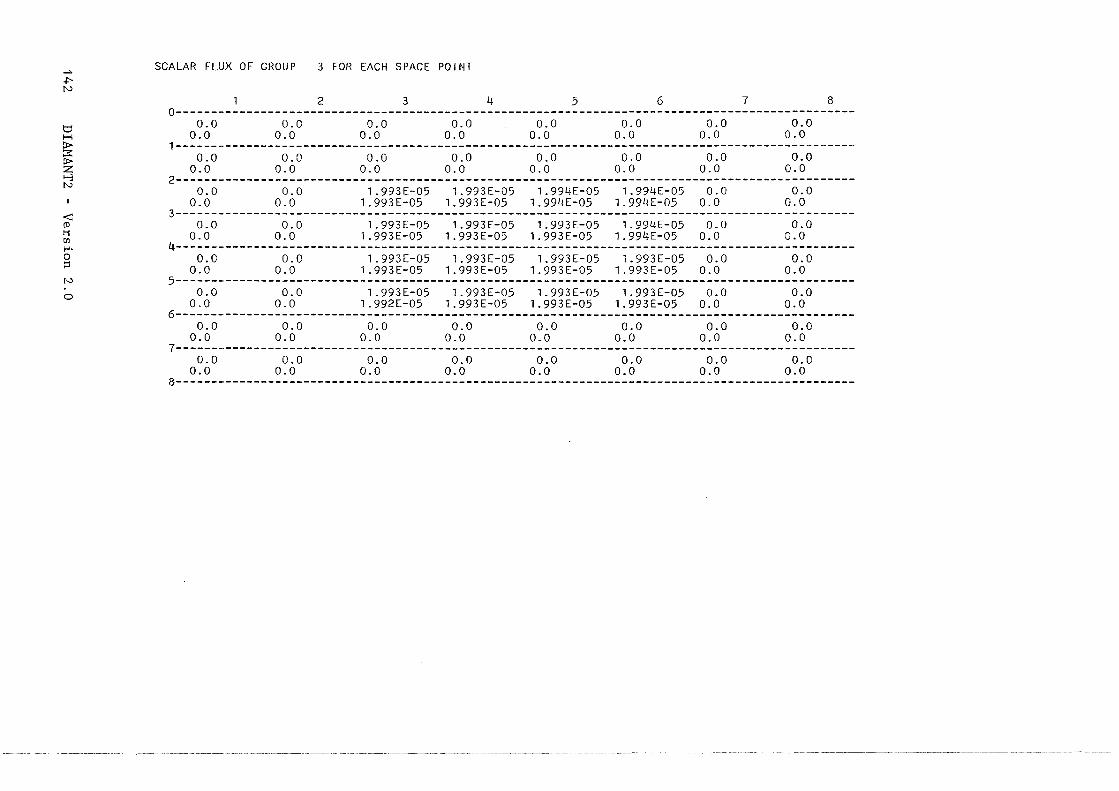
~ N

t::i H > 3: > z >-3 N

< (I)

1-1 Cll .... 0 ~

N

0


1 2 3 4 5 6 7 8 0--------------------------------------------------------------------------------------·----------o.o 0.0 0.0 0.0 0.0 0.0 0.0 0.0

0.0 0.0 0.0 0.0 0.0 0.0 0.0 0.0 1------------------------------------------------------------------------------------------------o.o 0.0 0.0 0.0 0.0 0.0 o.o 0.0

0.0 0.0 0.0 0.0 0.0 0.0 0.0 0.0 2------------------------------------------------------------------------------------------------o.o 0.0 1.993E-05 1.993E-05 1.994E-05 1.994E-05 0.0 0.0

0.0 0.0 1.993E-05 1.993E-05 1.994E-05 1.994E-05 0.0 0.0 3------------------------------------------------------------------------------------------------o.o 0.0 1.993E-05 1.993E-05 1.993E-05 1.994E-05 0.0 0.0

0.0 0.0 1.993E-05 1.993E-05 1.993E-05 1.994E-05 0.0 0.0 4------------------------------------------------------------------------------------------------o.o 0.0 1.993E-05 1.993E-05 1.993E-05 1.993E-05 0.0 0.0

0.0 0.0 1.993E-05 1.993E-05 1.993E-05 1.993E-05 0.0 0.0 5------------------------------------------------------------------------------------------------o.o 0.0 1.993E-05 1.993E-05 1.993E-05 1.993E-05 0.0 0.0

0.0 0.0 1.992E-05 1.993E-05 1.993E-05 1.993E-05 0.0 0.0 6------------------------------------------------------------------------------------------------o.o 0.0 0.0 0.0 0.0 0.0 0.0 0.0

0.0 0.0 0.0 0.0 0.0 0.0 0.0 0.0 7------------------------------------------------------------------------------------------------o.o 0.0 0.0 0.0 0.0 o.o 0.0 0.0

0.0 0.0 0.0 0.0 0.0 0.0 0.0 o.o 8------------------------------------------------------------------------------------------------

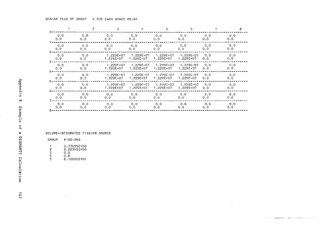
:J> "0 "0

~ 0.. f-'· ~

td

t%'J X 0>

-ä f-' (D

0 t-h

ill

t:1 H :J> ::3:: :J>

~ N

0 0> f-' (")

~ ....... ill rt f-'· 0 ::I

~ (.,)


1 2 3 4 5 6 7 8 0------------------------------------------------------------------------------------------------o.o 0.0 0.0 0.0 0.0 0.0 0.0 0.0

0.0 0.0 0.0 0.0 0.0 0.0 0.0 0.0 1------------------------------------------------------------------------------------------------o.o 0.0 0.0 0.0 0.0 0.0 0.0 0.0

0.0 0.0 0.0 0.0 0.0 0.0 0.0 0.0 2------------------------------------------------------------------------------------------------o.o 0.0 1.229E-07 1.229E-07 1.229E-07 1.229E-07 0.0 0.0

0.0 0.0 1.229E-07 1.229E-07 1.229E-07 1.229E-07 0.0 0.0 3------------------------------------------------------------------------------------------------o.o 0.0 1.229E-07 1.229E-07 1.229E-07 1.229E-07 0.0 0.0

0.0 0.0 1.229E-07 1.229E-07 1.229E-07 1.229E-07 0.0 0.0 4------------------------------------------------------------------------------------------------o.o 0.0 1.229E-07 1.229E-07 1.229E-07 1.229E-07 0.0 0.0

0.0 0.0 1.229E-07 1.229E-07 1.229E-07 1.229E-07 0.0 0.0 5------------------------------------------------------------------------------------------------o.o 0.0 1.229E-07 1.229E-07 1.229E-07 1.229E-07 0.0 0.0

0.0 0.0 1.229E-07 1.229E-07 1.229E-07 1.229E-07 0.0 0.0 6------------------------------------------------------------------------------------------------o.o 0.0 0.0 0.0 0.0 0.0 0.0 0.0

0.0 0.0 0.0 0.0 0.0 0.0 0.0 0.0 7------------------------------------------------------------------------------------------------o.o 0.0 0.0 0.0 0.0 0.0 0.0 0.0

0.0 0.0 0.0 0.0 0.0 0.0 0.0 0.0 8------------------------------------------------------------------------------------------------

VOLUME-INTEGRATED FISSION SOURCE

GROUP FISSIONS

1 0.77655E+OO 2 0.22345E+OO 3 0.0 4 0.0 5 0.10000E+01

~ ~

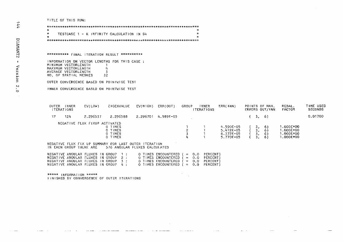
t::l H 0> ;:;:: 0>

~ N

<: (!) ti [Jl

1-'· 0 l:l

N

0

TITLE OF THIS RUN:

********************************************************************** * * *

TESTGASE 1 - K INFINITY GALGULATION IN S4 * * *

**********************************************************************

********** FINAL ITERATION RESULT **********

INFORMATION ON VEGTOR MINIMUM VEGTORLENGTH MAXIMUM VEGTORLENGTH AVERAGE VEGTORLENGTH NO. OF SPATIAL MESHES

LENGTHS 1 4 3

32

FOR TH I S GASE :

OUTER GONVERGENGE BASED ON POINTWISE TEST

INNER GONVERGENGE BASEDON POINTWISE TEST

OUTER INNER ITERATIONS

EV(LOW) EIGENVALUE EV(HIGH) ERR(OUT) GROUP INNER ERR( INN)

12 124 2.296537 2.296588

NEGATIVE FLUX FIXUP AGTIVATED 0 TIMES 0 TIMES 0 TIMES 0 TIMES

2.296701 4.989E-05

2 3 4

NEGATIVE FLUX FIX UP SUMMARY FOR LAST OUTER ITERATION IN EAGH GROUP THERE ARE 576 ANGULAR FLUXES GALGULATED

NEGATIVE ANGULAR FLUXES IN GROUP 1 0 TIMES ENCOUNTERED ( = NEGATIVE ANGULAR FLUXES IN GROUP 2 0 TIMES ENGOUNTERED ( = NEGATIVE ANGULAR FLUXES IN GROUP 3 0 TIMES ENCOUNTERED ( = NEGATIVE ANGULAR FLUXES IN GROUP 4 0 TIMES ENGOUNTERED ( =

***** INFORMATION ***** FINISHED BY GONVERGENGE OF OUTER ITERATIONS

ITERATIONS

0.0 PERGENT) 0.0 PERGENT) 0.0 PERGENT) 0.0 PERGENT)

4.590E-05 5.412E-05 6.372E-05 5.770E-05

POINTS OF MAX. ERRORS OUT/INN

3, 6)

3, 6) 3, 6) 3, 6) 3, 6)

REBAL. FAGTOR

l.OOOE+oo 1.000E+OO 1.oooE+oo l.OOOE+oo

TIME USED SECONDS

0.01700

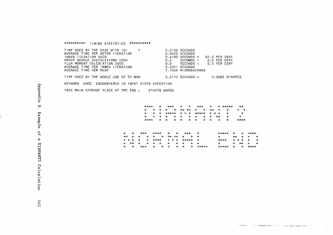
> "0 "0 (I) ::l p,. 1-'· X

t:P

t:%j

X lll 8 "0 I-' (I)

0 t-h

lll

t::l H

~ > z 1-3 N

0 lll I-' 0 ~ I-' lll rt 1-'· 0 ::l

-1'-Ln

********** TIMING STATISTICS **********

TIME USED BY THE CASE WITH ID= AVERAGE TIME PER OUTER ITERATION INNER ITERATION USED GROUP SOURCE CALCULATIONS USED FLUX MOMENT CALCULATION USED AVERAGE TIME PER INNER ITERATION AVERAGE TIME PER MESH

TIME USED BY THE WHOLE JOB UP TO NOW

0.5100 SECONDS 0.0425 SECONDS 0.4190 SECONDS = 0.0 SECONDS = 0.0 SECONDS = 0.0041 SECONDS 7.1404 MICROSECONDS

0.5110 SECONDS = KEYWORD ENDE ENCOUNTERED IN INPUT STOPS EXECUTION

FREE MAIN STORAGE PLAGE AT THE END : 214378 WORDS

**** * *** * * *** * * * * * ** ** * * * * * ***** * * * ***** * * * * * * * * * **** * * * * * * *

* * *** **** * * *** * ** * * * * * ** ** * * * * * * * * **** * * * ***** * * ** * * * * * * * * *

82.2 PER CENT 0.0 PER CENT 0.0 PER CENT

0.0085 MINUTES

* * ***** ** ** * * * * * * * * * * ** * * * * * ****

***** * * * ** * **** * * * * * **

* * *** * * * * * * ***** ***** * *

**** * * * * * * ****

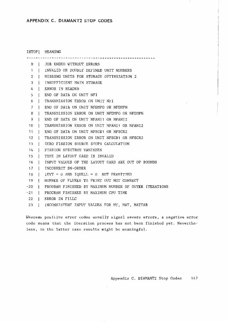
APPENDIX C. DIAMANT2 STOP CODES

ISTOPI NEANING

0 JOB ENDED WITHOUT ERRORS

1 INVALID OR DOUBLY DEFINED UNIT NUHBERS

2 NISSING UNITS FOR STORAGE OPTINIZATION 2

3 INSUFFICIENT MAIN STORAGE 4 ERROR IN READKO

5 END OF DATA ON UNIT NFI 6 TRANSHISSION ERROR ON UNIT NFI

7 END OF DATA ON UNIT NFDHPO OR NFDHPN

8 TRANSHISSION ERROR ON UNIT NFm!PO OR NFm!PN

9 END OF DATA ON UNIT NFANI1 OR NFANI2 10 TRANSHISSION ERROR ON UNIT NFANI1 OR NFANI2

11 END OF DATA ON UNIT NFSCR1 OR NFSCR2 12 TRANSHISSION ERROR ON UNIT NFSCR1 OR NFSCR2 13 ZERO FISSION SOURCE STOPS CALCULATION

14 FISSION SPECTRUH VANISHES

15 TYPE IN LAYOUT CARD IS INVALID 16 INPUT VALUES OF THE LAYOUT CARD ARE OUT OF BOUNDS

17 INCORRECT SN-ORDER 18 IEVT = 0 AND IQUELL = 0 NOT PERHITTED 19 NUMBER OF FLUXES TO PRINT OUT NOT GORREGT

-20 PROGRAN FINISRED BY MAXIHUM NUHBER OF GUTER ITERATIONS -21 PROGRAM FINI SHED BY MAXH!UH CPU TIHE

22 ERROR IN FILLC 23 INCONSISTENT INPUT VALUES FOR ~!T, HAT, MATTAB

Whereas positive error codes usually signal severe errors, a negative error code means that the iteration process has not been finished yet. Neverthe

less, in the latter case results might be meaningful.

Appendix C. DIAHANT2 Stop Codes 147

ACKNOWLEDGMENTS

The authors want to thank B.delMarmol and G.Minsart for providing the very

first version of the code. Special thanks are due to E.Kiefhaber who accom

panied our efforts with helpful discussions and support. Especially, he has

influenced the re-design of the iteration strategy and also put much time

in carefully reviewing the many drafts of this reports. Many thanks are due

to R.Böhme, C.Broeders, I.Broeders, G.Buckel, H.Giese, A.Polch and D.Thiem

for useful remarks concerning the draft version of this report. Special

thanks are due to J.Marek for his help with some of the figures. D.Sanitz

at KfK, GSI Darmstadt, KFA Jülich and the universities of Karlsruhe and

Kaiserslautern helped in providing access to the different vector computers.

Acknowledgments 149

150 DIANANT2 - Version 2.0

RE FE RENCES

/1/ K.Küfner, R.Heger,

"DIM!ANT2 - Ein Hultigruppen Neutronentransportprogramm für Dreiecks

und Hexagonalgeometrie",

KfK 3033, Karlsruhe 1980 (in German; english translation available from

RSIC)

/2/ K.Küfner, B.DelHarmol, G.Hinsart,

"Continuous Four Point Triangular ~!esh Difference Schemes for the Hul

tigroup Neutron Transport Equation",

Proc. Top. ~ieeting on Computational Hethods, pp.4-35 to 4-47, \Hl

liamsburg 1979

/3/ K.Kobayashi, G.Buckel, K.Klifner,

"TPTRIA, A Computer Program for the Reactivity and Kinetic Parameters

for T~·JO-Dimensional Triangular Geometry by Transport Perturbation

Theory",

KfK 4116, Karlsruhe 1986

/4/ G.Buckel, W.Höbel,

"Das Karlsruher Programmsystem KAPROS, Teil 1",

KfK 2253, Karlsruhe 1976 (in German; english translation: Risley Trans

5016, UKAEA 1976)

/5/ K.D.Lathrop, F.W.Brinkley,

"T\vOTRAN-II: An Interfaced, Exportahle Version of the T\VOTRAN Code for

Two-Dimensional Transport",

LA-4848-HS, Los Alamos 1973

/6/ W.F.Walters et al.,

Trans. Am. Nucl. Soc., 28, 257 (1978)

/71 B.G.Carlson,

"Tables of Equal Weight Quadrature EQN Over the Unit Sphere"

LA-4743, Los Alamos 1971

/8/ E.E. Lewis, W.F. Hiller,Jr.

"Computational Hethods of Neutron Transport"

Wiley & Sons New York, 1984

/9/ K.Klifner,

"READKO - Ein Unterprogrammpaket für zentralisierte Ein- und Ausgabe

operationen in KAPROS (Version(1 .8)) 11

KfK 3333, Karlsruhe 1982 (in German)

References 151

/10/ K.Küfner,

unpublished note,1986 (in German)

/11/ H.Bachmann, D.Sanitz,


/12/ H.Borgwaldt,


/13/ "RXVP80 - The Verification and Validation System for FORTRAN",

Version 4.0, User's manual

General Research Corp., Santa Barbara, California, 1985

/14/ K.Küfner, J.Burkhard, R.Heger,

"A Set of Test Gases for the 2-d Static Neutron Transport Code DIAHANT2

for Regular Triangular Geometry",

report in preparation (1987)

/15/ International Organization for Standardization,

"Programming Language FORTRAN",

ISO 1539-1980 or ANSI X3.9-1978,

/16/ Cyber 205 Service,

"VAST Automatie Vectorizer User Guide",

Control Data 1983


An Updated F RTRAN-77 Version of the 2-D Static Neutron ...

Documents

Transcript of An Updated F RTRAN-77 Version of the 2-D Static Neutron ...