An Update of the Analytical Groundwater Modeling to...

iii

CONTENTS

Notation...................................................................................................................................v

Acknowledgments................................................................................................................ vii

1 Introduction .........................................................................................................................1

1.1 The Bureau of Land Management’s Solar Energy Program ........................................1 1.2 The Afton Solar Energy Zone ......................................................................................2

2 Hydrogeologic Setting And Model Input Parameters .........................................................5

2.1 Aquifer Characteristics .................................................................................................5 2.2 Hydraulic Conductivity and Storage Properties ...........................................................6 2.3 Summary and Evaluation of the LRG Model ...............................................................7

3 Methodology .....................................................................................................................11

3.1 Approach ....................................................................................................................11 3.2 Pumping Rates ............................................................................................................12 3.3 Base-Case Aquifer Parameter Values ........................................................................13

4 Results and Discussion .....................................................................................................15

4.1 Afton SEZ Analytical Modeling ................................................................................15 4.1.1 Unconfined Aquifer Scenario ......................................................................15 4.1.2 Confined Aquifer Scenario ..........................................................................17

4.2 Discussion and Summary ...........................................................................................18 4.3 Implications for Future Model Development .............................................................19

5 References .........................................................................................................................21

TABLE

1 Low-, Medium-, and High-Demand SEZ Groundwater Pumping Requirements

Assumed for the Afton SEZ .............................................................................................. 13

iv

FIGURES 1 General Terrain of Afton SEZ ............................................................................................ 3 2 Generalized Geologic Cross Section across Mesilla Basin near the Afton SEZ ................ 6

APPENDICES

A Results for Unconfined Aquifer .......................................................................................23

B Results for Confined Aquifer ...........................................................................................31

v

NOTATION The following is a list of acronyms, initials, symbols, and abbreviations (including units of measure) used in this document. Acronyms, Initials, Symbols and Abbreviations BLM Bureau of Land Management b aquifer thickness DOE U.S. Department of Energy K hydraulic conductivity LRG Lower Rio Grande (groundwater model) PEIS programmatic environmental impact statement PV photovoltaic SEZ solar energy zone SSPA S.S. Papadopulos & Associates, Inc. Sy specific yield T aquifer transmissivity Units of Measure ac-ft acre-feet cm centimeter(s) d day ft feet ft3 cubic feet km kilometers km2 square kilometers m meters m2 square meters s second yr year

vi

This page intentionally left blank

vii

ACKNOWLEDGMENTS We wish to thank Peggy Barroll of the New Mexico Office of the State Engineer and Sarah Falk of the U.S. Geological Survey for their assistance in acquiring the Lower Rio Grande model for review. We would also like to thank Larisa Ford, Lee Koss, Paul Summers, and Ray Brady of the Bureau of Land Management (BLM) for providing guidance and oversight for the groundwater modeling project associated with BLM’s Solar Energy Program. The work was funded by the BLM National Renewable Energy Coordination Office under an interagency agreement, through U.S. Department of Energy contract DE-AC02-06CH11357.

viii


1

AN UPDATE OF THE ANALYTICAL GROUNDWATER MODELING TO ASSESS WATER RESOURCE IMPACTS AT THE AFTON SOLAR ENERGY ZONE – DRAFT REPORT

John J. Quinn, Christopher B. Greer1, and Adrianne E. Carr

Environmental Science Division Argonne National Laboratory

Argonne, IL

1 INTRODUCTION The purpose of this study is to update a one-dimensional analytical groundwater flow model to examine the influence of potential groundwater withdrawal in support of utility-scale solar energy development at the Afton Solar Energy Zone (SEZ) as a part of the Bureau of Land Management’s (BLM’s) Solar Energy Program. This report describes the modeling for assessing the drawdown associated with SEZ groundwater pumping rates for a 20-year duration considering three categories of water demand (high, medium, and low) based on technology-specific considerations. The 2012 modeling effort published in the Final Programmatic Environmental Impact Statement for Solar Energy Development in Six Southwestern States (Solar PEIS; BLM and DOE 2012) has been refined based on additional information described below in an expanded hydrogeologic discussion. 1.1 The Bureau of Land Management’s Solar Energy Program In 2012, the BLM officially established its Solar Energy Program, which facilitates permitting of utility-scale solar energy development on BLM lands in six southwestern states (Arizona, California, Colorado, Nevada, New Mexico, and Utah) in an environmentally responsible manner (BLM 2012). As a part of the Solar Energy Program, the BLM established SEZs, which are areas that are well-suited for utility-scale production of solar energy where BLM will prioritize solar development. The BLM, together with the U.S. Department of Energy (DOE), analyzed the potential environmental impacts of the Solar Energy Program in the Solar PEIS (BLM and DOE 2012), including impacts on water resources. Groundwater is the primary water resource available for solar energy development in most of the SEZs, and impacts of groundwater withdrawals were investigated qualitatively and semi-quantitatively in the Solar PEIS to assess the range of potential effects. Impacts of reduced magnitude and timing of groundwater flows to streams, springs, seeps, and wetlands would depend upon the connectivity of surface water and groundwater in the region. These impacts include decreased water supply for downstream users; loss of wetland vegetation species; and loss of habitat and forage for wildlife, wild horses, and livestock.

1 Now at Fermilab, Batavia, Illinois.

2

As a part of the Solar PEIS analysis, water requirements for cooling and/or washing uses at solar energy facilities were examined for different technologies and varying levels of development and compared with basin-scale water budgets. In addition, one-dimensional groundwater modeling was performed to examine potential radial drawdown for different solar development scenarios. As a follow-on to the work done for the Solar PEIS, BLM identified a subset of SEZs, including the Afton SEZ, for further analysis and groundwater modeling. The analyses are being used to examine potential groundwater impacts associated with future solar development of the SEZs, with a particular focus on examining groundwater drawdown and potential loss of connectivity to surface water features, springs, and vegetation. In addition to these analyses, the developed numerical or analytical groundwater models are being made available through the Solar PEIS Web site (http://blmsolar.anl.gov) so that they can be used for project-scale review and for the development of long-term monitoring programs. 1.2 The Afton Solar Energy Zone As described in the Final Solar PEIS (BLM and DOE 2012), the revised Afton SEZ has a developable area of 29,964 acres (121.2 km2) (Figure 1). It is oriented in a northwest-southeast direction, with overall dimensions of about 16 miles (26 km) by 4 miles (6 km). Its easternmost point is about 4 miles (6 km) west of the Rio Grande River. The SEZ has surface elevations that range between approximately 4,380 ft (1,335 m) in the northwest and 4,210 ft (1,283 m) in the southeast.

3

Figure 1 General Terrain of Afton SEZ (Source: Modified from BLM and DOE 2012)

4


5

2 HYDROGEOLOGIC SETTING AND MODEL INPUT PARAMETERS The geologic and hydrologic setting of the Afton SEZ is described in the Final Solar PEIS (BLM and DOE 2012). Further details are included in the Draft Solar PEIS (BLM and DOE 2010). Key information is summarized below. 2.1 Aquifer Characteristics The Afton SEZ is situated in the West Mesa of the Mesilla Basin. Groundwater is in Quaternary and Tertiary age basin fill sediments known as the Santa Fe Group (Figure 2). The Santa Fe Group has a range of textures associated with distal, medial, and proximal alluvial fan deposits and also fluvial, basin floor fluvial, playa, and eolian deposits (Hawley and Kennedy 2004). In general, the upper Santa Fe Group is composed of ancestral Rio Grande channel sand and gravel; the middle unit is clean sand interbedded with silty clay; and the lower unit consists of fine-grained sediments that are partially consolidated. Because of cementation and the presence of fine-grained beds, the middle unit is less permeable than the upper unit; however, the middle unit is the major aquifer of the Mesilla Basin because it is saturated almost everywhere. Hawley et al. (2001) describe the upper Santa Fe Group as being the most productive, but also mostly unsaturated. Shallow portions of the Mesilla Basin valley fill may be unconfined, but essentially all aquifer zones greater than 200 ft (60 m) below the potentiometric surface are confined or semi-confined (Hawley and Kennedy 2004). The East Robledo fault is a north-northeast trending fault that bounds the western edge of the Mesilla structural basin (Figures 1 and 2). The fault trends through the Afton SEZ, with most of the SEZ on the valley side of the fault. The Tertiary volcanic and volcaniclastic basement is much closer to the surface west of the fault line, and the Santa Fe Group sediments are consequently relatively thin. Though the Santa Fe Group sediments to the west may be saturated, they do not have the appreciable thickness that is present east of the fault line, where the basement is much deeper. For this reason, the fault line is considered a Mesilla Basin boundary in several numerical groundwater flow models (Frenzel 1992; Frenzel and Kaehler 1992; SSPA 2007, 2008). Figure 1 illustrates the location of the East Robledo fault according to Frenzel and Kaehler (1992). Hydraulic heads in the Santa Fe Group in 1985 ranged from about 4,050 ft (1,230 m) in the northwest portion of the SEZ to about 3,830 ft (1,170 m) in the southeast portion (Nickerson and Myers 1993). Data from 1976 indicate about 3,880 ft (1,180 m) in the northwest portion of the SEZ and 3,820 ft (1,160 m) in the southwest portion of the SEZ (Wilson et al. 1981). These differences may be attributable to interpretation in the contouring of an area of sparse data such as West Mesa.

6

Figure 2 Generalized Geologic Cross Section across Mesilla Basin near the Afton SEZ (Source: Modified from Frenzel and Kaehler 1992) Hawley et al. (2001) shows heads at the SEZ of about 3,860 ft (1,180 m). According to cross sections of Hawley and Kennedy (2004), this water level would be approximately near the contact between upper and middle Santa Fe Group sediments. Groundwater flow in the Mesilla Basin is southeasterly, in parallel with the Rio Grande River. The hydraulic gradient is about 0.0001. Little groundwater is withdrawn in the West Mesa area (Nickerson and Myers 1993). Because of the great thickness of basin fill aquifer materials in the Mesilla Basin, the Santa Fe Group fill material east of the East Robledo fault was assumed to be the aquifer supplying water for SEZ operations. The thin saturated zone west of the fault was assumed to be unreliable as a long-term source of water for operations. The SEZ vicinity is several miles west of the topographically lower Rio Grande Valley, where a relatively thin alluvial aquifer is present in the river’s floodplain. 2.2 Hydraulic Conductivity and Storage Properties Frenzel (1992) assembled a large amount of aquifer test data in the Mesilla Basin and analyzed the information in terms of specific units within the Santa Fe Group. He described the hydraulic

7

conductivity (K) of the upper Santa Fe Group as 2 to 68 ft/d (7×10-4 to 2×10-2 cm/s), the middle unit as 1 to 100 ft/d (4×10-4 to 4×10-2 cm/s) (with the shallower portion having higher values than the deeper portion), and the lower unit as 1 to 34 ft/d (4×10-4 to 1×10-2 cm/s). The maximum saturated thickness of the Santa Fe Group is about 2,500 ft (760 m). The specific yield (Sy) of the unconfined aquifer is about 0.2, while the specific storage of confined zones is about 1.0×10-6 ft-1 (3×10-7 m-1). Hawley and Kennedy (2004) summarize information about West Mesa in the Mesilla Basin. Storativity was estimated to be 2×10-5. K values may be 70 ft/d (2×10-2 cm/s) in the uppermost part of the groundwater flow system but decrease with depth. A median value of 66 ft (20 m) was determined for the upper 600 ft (180 m) of saturated sediment associated with the upper and uppermost middle units of the Santa Fe Group. A median of 5 ft/d (2×10-3 cm/s) was determined for the middle and lower units of the Santa Fe Group. In the overall Mesilla Basin, the Sy is 0.1 to 0.2, while the specific storage of confined aquifers is 1×10-5 to 1×10-6 ft-1 (3×10-6 to 3×10-7 m-1) or storativity of 2×10-3 to 3×10-5 (Hawley and Kennedy 2004). The K values used in the LRG model are described in Section 2.3. 2.3 Summary and Evaluation of the LRG Model A recent, detailed model of the Lower Rio Grande (the LRG model), which includes the Mesilla Basin and surrounding areas, was evaluated for its use in assessing the drawdown that would be associated with pumping at the Afton SEZ. The model was produced by S.S. Papadopulos & Associates, Inc. (SSPA) for the New Mexico Attorney General, the New Mexico Office of the State Engineer, and the New Mexico Interstate Stream Commission. The project was guided by a technical committee consisting of members of the above state offices, consultants (including SSPA), and academics, and is documented in a set of reports (SSPA 2007, 2008). The calibrated version of this model (file set LRG_2007a) was provided to Argonne National Laboratory by Peggy Barroll (New Mexico Office of the State Engineer) on April 26, 2013. The model domain is located along the Rio Grande River across portions of New Mexico, Texas, and Mexico. The region extends from the Caballo Dam in the north, through both the Rincon Valley and Mesilla Valley. The model replaced prior models of the region with particular improvements, including reliance on a recent geologic model; updated pumping information for irrigation, municipal, and industrial uses; and detailed modeling of streams, canals, and drains. The LRG model’s study area is part of the Rio Grande Project, an extensive system of dams, canals, and drains for agricultural purposes (SSPA 2007). The hydrogeological framework of the model is comprised of alluvium in the two valleys and the upper, middle, and lower Santa Fe formation beneath the valleys and in the surrounding uplands. The western boundary of the LRG model coincides with the northeast-southwest trending East Robledo fault (Frenzel and Kaehler 1992). Here, the boundary of the Santa Fe Group sediments and the underlying Tertiary volcanic and volcaniclastic rocks has an abrupt change, with much thicker Santa Fe Group materials toward the river valley and shallower Santa Fe Group materials

8

atop the volcanics to the west of the fault. Available hydraulic head data (Hawley and Kennedy 2004) suggest a very thin saturated zone in the Santa Fe Group sediments west of the fault. Most of the SEZ is located east of the East Robledo fault, over deep Santa Fe Group sediments. The southwest edge of the modeling domain is the Potrillo fault, which intersects the East Robledo fault (Frenzel and Kaehler 1992). Water inputs to the LRG study area are dominated by Rio Grande River flow. Other inputs, which combined are at least two orders of magnitude less than the river flow, are groundwater inflow, mountain front recharge, and precipitation (SSPA 2007). Outputs include irrigation and municipal well pumping, riparian evapotranspiration loss, crop evapotranspiration, surface water evaporation, and transbasin groundwater discharge at the south end of the Mesilla Basin. Modeling of the LRG model was conducted using MODFLOW 2000 (Harbaugh et al. 2000) and the Layer Property Flow option. The three-dimensional model grid (SSPA 2007) is comprised of grid cells that are 0.25 mile (402 m) on each side, and so measure 40 acres (16 ha) in area. The grid has five layers. Layer 1 is comprised of Rio Grande alluvium in the river valley and upper Santa Fe formation away from the river. Near the SEZ, Layers 2 and 3 represent the upper Santa Fe formation sediments while Layer 4 is middle Santa Fe Group sediments and Layer 5 is middle and lower Santa Fe Group sediments. The top four layers represent units less than 600 feet (183 m) below the river elevation, where the bulk of groundwater flow takes place. Layer 5 is Santa Fe formation deeper than 600 feet (183 m) below the river elevation. The bottom of the model is bounded by an estimated surface of low-permeability formations deeper than the Santa Fe Group sediments. Aquifer parameter distributions throughout the model layers were based on published data and were reviewed by the state’s technical committee (SSPA 2007). Model Layer 1 is a saturated unconfined layer 70 feet (20 m) thick near the Rio Grande River, and it thickens away from the river valley area (SSPA 2008). Layers 2, 3, and 4 are confined layers 130 ft (40 m), 200 ft (60 m), and 200 ft (60 m) thick, respectively. Layer 5 is confined and ranges from 130 ft (40 m) to almost 2,000 ft (610 m) thick. Details of model design, input (aquifer parameters, pumping stresses, recharge, surface water modeling), and calibration are described in SSPA (2007, 2008) and are not reproduced here. Model development initially considered pumping stresses from primary and secondary irrigation seasons prior to expanded agricultural pumping beginning in 1940 (SSPA 2007). This analysis, which relied on a small number of available calibration targets, produced what is considered the pre-development conditions from 1940 to 2004. Stress periods alternated between an eight-month irrigation season and a four-month non-irrigation season. Calibration targets included water levels in wells, drain flows, and canal leakage. Sensitivity analyses conducted by SSPA (2007) indicated that the model is most sensitive to hydraulic conductivity values in Layers 1 and 2 and by conductance values assigned to rivers/canals/drains. The LRG model is a valuable tool for many types of groundwater analyses in the Rincon and Mesilla valleys, especially close to the Rio Grande River where the model is more detailed and

9

supported with data. However, it was not used in this study to evaluate the additional drawdown that would occur due to SEZ groundwater pumping for several reasons. The LRG model runs a proprietary riparian evaporation package that is not recognized by other MODFLOW-based programs. Even with this option turned off during model runs, model calculations stopped part-way through due to unknown errors. Although it is accompanied by its own executable MODFLOW program, the output from this program is not compatible with other MODFLOW graphical user interfaces. Furthermore, its lengthy run times would be prohibitive for evaluating drawdown differences at the SEZ, in particular because the SEZ area is far from the locations of hard data available on aquifer parameters.,The LRG model was not used to assess drawdown at the Afton SEZ because of these complications. Instead, an analytical method was applied to test the drawdown effect at the SEZ over a range of plausible aquifer conditions and parameter values. The analytical model input (see Section 3) is derived from a review of basin literature information combined with input values from the LRG model specific to the SEZ area. In the LRG model, a small portion of the northwestern end of the SEZ is west of the East Robledo fault and therefore out of the modeling domain. In the calibrated LRG model, the K of the remaining portion of Layer 1 was 5 to 10 ft/d (2×10-3 to 4×10-3 cm/s) in the central SEZ and 10 to 15 ft/d (4×10-3 to 5×10-3 cm/s) in the southeastern SEZ. In Layer 2, K was 15 to 40 ft/d (5×10-3 to 1×10-2 cm/s) in the central SEZ and 40 to 100 ft/d (1×10-2 to 4×10-2 cm/s) in the southeastern tip. In Layers 3 and 4, K was 10 to 15 ft/d (4×10-3 to 5×10-3 cm/s) in the central and southeastern SEZ (SSPA 2008). The calibrated LRG model relied on a layer 1 Sy value of 0.2 and specific storage values in Layers 2 through 5 of 1.2×10-5, 3.8×10-6, 2.5×10-6, 2.5×10-6 ft-1 (4.2×10-9, 1.3×10-9, 8.8×10-10, 8.8×10-10 m-1), respectively. LRG model parameter values were used as base-case input values in the analytical model, as described in Section 3.3.

10


11

3 METHODOLOGY 3.1 Approach The analytical modeling approach relies on simplifying assumptions to generate a distance-drawdown relationship based on a combination of input parameters (pumping rate, hydraulic conductivity, aquifer thickness, pumping duration, and aquifer storage). The analytical modeling method is also described in Appendix O of BLM and DOE (2012). Drawdown of the potentiometric surface due to radial groundwater flow to a pumping well can be estimated using analytical equations and simplifying assumptions. This method can be applied to a confined aquifer. The solution relates drawdown to an infinite-series term called the well function,

4 0.5772 / 2 2! / 3 3! / 4 4! ⋯ ,

where the argument u is

4

and Q = constant pumping rate [volume/time] h = hydraulic head at time t since pumping began [length] ho = hydraulic head prior to pumping [length] r = radial distance from the pumping well to an observation well [length] T = aquifer transmissivity [length2/time] S = aquifer storativity [unitless]. Transmissivity is the product of the aquifer’s hydraulic conductivity, K [length/time], and the aquifer’s thickness, b [length]. Storativity for a confined aquifer is the product of the specific storage and the aquifer thickness, and is usually small (<0.005). Assumptions of this method include a constant pumping rate, Darcian flow, and instant release of water from storage (Fetter 1988). The aquifer is assumed to be homogenous, isotropic, of a constant thickness, of negligible slope, and of infinite extent. The pumping well and observation wells are assumed to penetrate the aquifer fully, and the pumping well’s diameter is infinitesimal. For this study, the drawdown to be evaluated occurs as a result of long-term pumping. The Jacob method acknowledges that when u of the equation is very small (e.g., time t is very large), the equation can be truncated after the first two terms (Fetter 1988), such that the equation becomes

. . .

12

This step is valid when u <0.01, and for most applications, is valid if u <0.1 (Halford and Kuniansky 2002). For unconfined aquifers, three phases of time-drawdown relationships occur during pumping (Fetter 1988). Initially, the aquifer contributes a small amount of water due to release from storage consistent with the equation. Continued pumping causes a transition to decline of the water table due to gravity drainage. In the later stage, the situation transitions to a decreasing rate of drawdown, and time-distance data can again be modeled with the equation (Kruseman and DeRidder 2000). Because this late-stage scenario is what is considered in the 20 year-long Solar PEIS analyses, the above equation is appropriate. In this case, however, the storage term to be used is the specific yield, Sy. Values of Sy for silts, sands, and gravels are generally in the range of 0.18 to 0.27 (Fetter 1988). For this project, a spreadsheet tool was developed to evaluate the drawdown at various distances from a pumping well at long time duration using the Jacob method. The model relies on user input that is provided in consistent units for length and time to evaluate drawdown at various distances while also displaying u values to check the validity of the approach. Depending on the hydrogeologic conditions, the storage term may be considered storativity (small values for a confined aquifer) or specific yield (large values for an unconfined aquifer). The spreadsheet includes a graphical view of the drawdown across a range of distances. Because of the simplicity of the analytical approach, input values can be quickly and easily tested to estimate the effect of long-term pumping at various distances from a pumping well or pumping center. These estimates can be determined for best-guess and worst-case scenarios, based on the ranges of appropriate input values. The appropriateness of the simplifying assumptions, especially those related to the aquifer’s spatial characteristics, must be considered carefully. 3.2 Pumping Rates The operational water requirements for a proposed SEZ depend on the degree of buildout on the SEZ and the solar energy technology (BLM and DOE 2012). Some technologies require a cooling system, but all technologies require water for cleaning panels or mirrors. For the Afton SEZ, the considered low-, medium-, and high-demand groundwater pumping scenarios represent full buildout of the SEZ assuming photovoltaic (PV) panels, dry-cooled parabolic troughs, and wet-cooled parabolic troughs, respectively (BLM and DOE 2012). Dry- and wet-cooled power tower facility water use can be assumed to be similar to that of dry- and wet-cooled parabolic trough facilities. These water requirements are summarized in Table 1. A range of values for an assumed 80% buildout of the SEZ was estimated for dry-cooled (3,423 to 7,258 ac-ft/yr, or 11,570 to 24,530 m3/d) and wet-cooled (24,038 to 71,980 ac-ft/yr, or 81,234 to 243,250 m3/d) concentrating solar power technologies (BLM and DOE 2012). The values at the low end of these ranges were selected for use in this drawdown analysis (presented

13

Table 1 Low-, Medium-, and High-Demand SEZ Groundwater Pumping Requirements Assumed for the Afton SEZ

Assumed Pumping Requirements

Description Pumping Scenario ac-ft/yr m3/d ft3/d

Full buildout of PV Low 136 460 16,220 Full buildout of dry-cooled

parabolic trough Medium 3,423 11,570 408,400

Full buildout of wet-cooled parabolic trough

High 24,038 81,234 2,867,700

in Table 1) because these represent a 30% capacity factor2 for solar facilities, which is much more likely than the 60% capacity factor represented by the upper end of the range. The model duration was 7,305 days, or 20 years. In this assessment, results are generated and compared for a single supply well vs. multiple supply wells scattered across the SEZ. 3.3 Base-Case Aquifer Parameter Values Because of a lack of site-specific information, two analytical model scenarios were examined: an unconfined aquifer and a confined aquifer. This decision was made because of the range of unconfined, semi-confined, and confined conditions present in the Mesilla Basin, where alluvial fan depositional processes may result in a significant unconfined aquifer and one or more significant confined aquifers. For the unconfined case, the base-case value for saturated thickness assigned in the analytical model was 100 ft (30 m). Base-case values for horizontal hydraulic conductivity (10 ft/d, or 3 m/d) and specific yield of 0.2 were assigned based on the SSPA (2008) model input. For the confined case, a base-case thickness of 200 ft (60 m) was tested (assuming a well screened across a 200-ft [60-m] thickness of aquifer materials with confining clay units above and below), along with a K value of 40 ft/d (12 m/d) and a storativity of 5×10-4. In both cases, the parameter values were consistent with the literature values available for the overall Mesilla Basin. The sensitivity of the model to these inputs was evaluated.

2 Capacity factor is a value representing the estimated actual annual operating hours for an electrical generating

facility. The values also assumed 5 acres/megawatt for parabolic trough facilities and 9 acres/megawatt for PV facilities as land area requirements.

14


15

4 RESULTS AND DISCUSSION 4.1 Afton SEZ Analytical Modeling 4.1.1 Unconfined Aquifer Scenario High-Demand Pumping at the SEZ In the unconfined aquifer scenario with high-demand SEZ pumping (assumes base-case values for horizontal hydraulic conductivity of 10 ft/d [4×10-3 cm/s] and for specific yield of 0.2), the calculated drawdown after 20 years was an impossible value of over 3,000 ft (900 m) after 20 years (Figure A-1). At a distance of a mile (1.6 km), the drawdown was about 250 ft (76 m). The assumed aquifer thickness would actually be completely dewatered in the well vicinity during the first month of operation, given the model input values. At a large SEZ property, it would be efficient to have multiple pumping wells arranged throughout the site to deliver water to various sectors, to reduce drawdown effects relative to those of a single well and to provide redundancy so that the water system can provide water if one or more wells are not operational due to pump maintenance or other issues. However, even if a system of five wells were installed, under the high-demand pumping scenario, the drawdown at each well would be impossibly large after 20 years (Figure A-2). If the single well case were adjusted favorably so that K was assumed to be 100 ft/d (4×10-2 cm/s) (which is outside the range of literature values) and the thickness was tripled to 300 ft (91 m), the calculated drawdown in the well vicinity would be over 100 ft (30 m) after 20 years (Figure A-3). This large drawdown could be attributed to the large water requirements for high-demand wet cooling. If a wellfield of five scattered wells were implemented, the drawdown at each well would be less than 30 ft (10 m) (Figure A-4), with combined drawdown at large distances similar to that shown in Figure A-3. These results suggest the importance of acquiring site-specific field characterization data, if an unconfined aquifer is present and investigated as a potential source of water to support operations. Several of the graphed results display a negative drawdown (e.g. Figures A-1 and A-2). This coincides with the value of u exceeding approximately 0.1, and, as described in Section 3, implies a relative lack of accuracy at large distances from the well location. Medium-Demand Pumping at the SEZ For the unconfined aquifer scenario using the base-case input values and dry-cooling technology (3,423 ac-ft/yr, or 11,570 m3/d), the drawdown by a single well after 20 years would be impossibly large, more than 400 ft (120 m) in the vicinity of the well (Figure A-5). If this pumping were distributed among five wells in the SEZ, the calculated drawdown would still be unreasonably large at each well, amounting to the full aquifer thickness (Figure A-6).

16

If the input parameters were adjusted as with the high-demand case (K increased beyond the range of published values to 100 ft/d, or 30 m/d, and thickness increased to 300 ft, or 90 m), the calculated drawdown after 20 years at a single well would be about 20 ft (6 m) at the well, and would be about 5 ft (1.6 m) at a distance of 1 mile (1.6 km) (Figure A-7). Multiple wells would have less drawdown at each well location, and their combined effect would result in a distant drawdown similar to that shown in Figure A-7. Low-Demand Pumping at the SEZ The assumed low-demand water requirement for PV is 136 ac-ft/yr (460 m3/d). With this pumping rate applied to a single well and with the base-case aquifer parameter input values, drawdown after 20 years would be less than 20 ft (6 m) in the well vicinity, about 3.5 ft (1.1 m) at a distance of 0.5 mile (0.8 km), and about 2 ft (0.6 m) at a distance of 1 mile (1.6 km) (Figure A-8). Modeling with more favorable aquifer parameter values and/or multiple wells would result in less drawdown. Sensitivity to Input Parameter Values Aquifer parameter values are expected to vary spatially. A means of assessing the effect of that variability on model output is to perform a sensitivity analysis on model input values. The parameters for hydraulic conductivity (K), specific yield (Sy), and aquifer thickness (b) were each adjusted by an amount reasonable for the hydrogeologic setting while holding the other parameters constant at the base-case level. For this sensitivity assessment, the medium-demand pumping case was analyzed because of the impractical output of the high-demand case and the small degree of impact of the low-demand case. Changes in K or b produced the same result, because they combine in the analytical model as the aquifer transmissivity (T) parameter. Conceptually, decreases in T (or K or b) are expected to produce a deep, localized cone of depression, whereas increases in T (or K or b) produce a shallower, broader cone of depression. Changes in Sy produce inverse results. The results are shown in Figure A-9. The base-case values tied to those of the SSPA (2008) numerical model produced impossibly large drawdown, as noted in the discussion of Figure A-5. Large changes in specific yield were found to have minimal effect on drawdown results. Relatively small changes (doubling or halving) in K or b produced much larger effects on drawdown; this is important because K can vary by orders of magnitude within a unit considered to be fairly homogenous. The order-of-magnitude increase in K produced significantly reduced drawdown. The order-of-magnitude decrease in K produced even more impossibly large drawdown; a production well would not be screened across such a low-K zone.

17

4.1.2 Confined Aquifer Scenario High-Demand Pumping at the SEZ For the high-demand case, use of the base-case aquifer input parameters given in Section 3.3 (i.e., base-case thickness of 200 ft (61 m), K value of 40 ft/d (12 m/d), and a storativity of 5×10-4) yielded drawdown values after 20 years that would be impossible large (Figure B-1). Even if pumping were distributed among five wells, the resulting potentiometric drawdown would be well over half of the aquifer’s thickness near each well (Figure B-2), likely creating unconfined conditions essentially throughout some portion of the Mesilla Basin. If aquifer parameters were more favorable, with a K value of 100 ft/d (30 m/d) (which is outside the range of literature values), and the assumed thickness were increased to 300 ft (91 m), drawdown at the well vicinity after 20 years would still be significant (Figure B-3), and large drawdown effects and likely unconfined conditions could result at large distances in the Mesilla Basin. If pumping were distributed among five well locations, drawdown would be up to 40 ft (12 m) at the well vicinity (Figure B-4). The compound effect of drawdown at distances from the five wells would be significant and would essentially match the distant values in Figure B-3. Medium-Demand Pumping at the SEZ In the case of medium demand and base-case aquifer input values, drawdown after 20 years at a single well is nearly 100 ft (30 m) at the well and about 31 ft (9.4 m) at a distance of 2 miles (3.2 km) (Figure B-5). Depending on aquifer conditions, the aquifer might convert to unconfined conditions close to the well, but may remain confined at a distance. If pumping were distributed among five pumping well locations, each well would show almost 20 ft (6 m) of drawdown near the well (Figure B-6), with distant drawdown similar to that shown in Figure B-5. If favorable conditions are assumed as in the high-demand analysis above, drawdown after 20 years at a single well is less than 30 ft (9 m) (Figure B-7). Both at the well and at a distance, aquifer conditions may remain confined depending on aquifer parameter values and other pumping in the region. This analysis again shows the importance of site-specific aquifer characterization data in assessing anticipated drawdown. Low-Demand Pumping at the SEZ For the low-demand PV case, with the base-case aquifer parameter estimates, drawdown at the well after 20 years would be less than 4 ft (1.2 m) (Figure B-8). Modeling with more favorable aquifer parameter values and/or multiple wells would result in less drawdown. Sensitivity to Input Parameter Values The sensitivity of the confined aquifer scenario was evaluated in a similar fashion to the unconfined aquifer above, but the storativity was evaluated by order-of-magnitude increases or decreases, consistent with the range of field values available for the Mesilla Basin. Again, the medium-demand case was selected for sensitivity analysis.

18

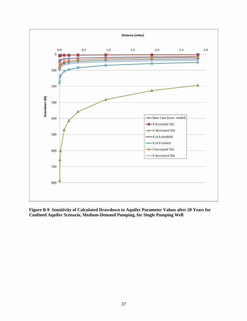
The results are shown in Figure B-9. The base-case values based on the SSPA (2008) numerical model produce a large amount of drawdown in the well vicinity, as described in the discussion of Figure B-5. The large tested range of S values had minor effect on calculated drawdown. Relatively small changes (doubling or halving) in K or b produced much larger effects on drawdown; this is important because K can vary by orders of magnitude within a unit considered to be fairly homogenous. The order-of-magnitude increase in K produced very minimal drawdown. The order-of-magnitude decrease in K produced impossibly large drawdown; a production well would not be screened across such a low-K zone. 4.2 Discussion and Summary This analytical method application gives support to the idea that the high-demand (wet-cooling technology) scenario for Afton SEZ water requirements would be impossible to sustain, even for a much shorter time frame than the 20-year period considered in this study. By applying the medium- and low-demand SEZ water requirements (Table 1), significantly smaller drawdowns are estimated, although the degree of drawdown from medium-demand operations would be significant. Based on literature values for the Mesilla Basin, the results indicate that an unconfined aquifer, if present, would be more susceptible to drawdown than a confined aquifer, because the expected larger K and b of the confined aquifer outweigh the effect of its smaller storage value. In both cases, however, the aquifer thickness and especially the distribution of hydraulic conductivity values in the subsurface are critical factors for evaluation of the anticipated drawdown. The medium-demand (dry-cooling technology) solar installation would produce infeasible drawdown results in the unconfined aquifer scenario, but with more favorable input values, more acceptable drawdown was calculated. For the medium-demand confined case, possible sustainability was indicated by the base-case parameter values, and likely sustainability was indicated, if aquifer conditions were more favorable. These cases suggest the importance of acquiring site-specific aquifer characterization data to determine whether a potential source of water could support operations. For a low-demand (PV) installation, drawdown is much less because the pumping rate is about 25 times less than the medium-demand case. A thorough understanding of the aquifer parameter values and their three-dimensional distribution becomes less critical in this situation. The infeasible high-demand pumping rate of 24,038 ac-ft/yr (81,234 m3/d) (Table 1) is quite large relative to the overall pumping in the region. In the combined Rincon and Mesilla valleys, agricultural pumping averages about 70,000 ac-ft/yr (236,000 m3/d) (SSPA 2008). Municipal, industrial, and domestic well pumping also takes place in those valleys, with the three largest withdrawals at the City of El Paso (up to about 23,000 ac-ft/yr, or 78,000 m3/d), the City of Las Cruces (up to about 20,000 ac-ft/yr, or 68,000 m3/d), and the Santa Teresa development (5,600 ac-ft/yr, or 19,000 m3/d) (SSPA 2008).

19

Pumping wells would likely be located on the SEZ property and east of the East Robledo fault. Depending on the locations of the pumping wells, their drawdowns may be greater than their analytically calculated drawdowns because of a boundary effect against the fault. Multiple pumping centers might be located across this large SEZ. The pumping stresses would be distributed among these different locations. The pumping rate at any well would of course be a portion of the total in Table 1, and drawdown in the immediate vicinity of individual wells would therefore be decreased. At greater distances, however, the resulting drawdown should be similar to what is modeled for a single well pumping. Determining whether water rights could be obtained to support SEZ groundwater requirements is beyond the scope of this study. The medium- and low-demand drawdown estimates may be useful in addressing concerns about water supply to other groundwater users in the basin and about downgradient ecological concerns related to spring flow or groundwater discharge to surface water bodies. 4.3 Implications for Future Model Development Improvements in the current model could be made with the discovery or collection of new data regarding the hydrogeological framework and aquifer parameter values. Drilling for production or monitoring wells, for example, could generate high-quality drill logs that could refine the hydrogeologic framework, provide water level data, and allow aquifer testing for determining parameter values in the local vicinity of the SEZ. The nature of the Santa Fe Group is such that it is highly variable spatially. Site-specific data would improve the design and accuracy about where such improvements are most needed for assessing drawdown impacts.

20


21

5 REFERENCES BLM and DOE (Bureau of Land Management and U.S. Department of Energy), 2010, Draft Environmental Impact Statement for Solar Energy Development in Six Southwestern States, DES 10-59, DOE/EIS-0403, prepared by Argonne National Laboratory, Environmental Science Division, Argonne, Illinois, December. BLM and DOE, 2012, Final Environmental Impact Statement for Solar Energy Development in Six Southwestern States, FES 12-24, DOE/EIS-0403, prepared by Argonne National Laboratory, Environmental Science Division, Argonne, Illinois, July. Volume 5, Section 12.1.9.2. BLM (Bureau of Land Management), 2012, Approved Resource Management Plan Amendments/Record of Decision (ROD) for Solar Energy Development in Six Southwestern States, Oct. Fetter, C.W., 1988, Applied Hydrogeology, 2nd edition, Merrill Publishing Company, Columbus, Ohio. Frenzel, P.F., 1992, Simulation of Ground-Water Flow in the Mesilla Basin, Doña Ana County, New Mexico, and El Paso County, Texas, Supplement to Open-Field Report 88-305, U.S. Geological Survey, Water-Resources Investigation Report 91-4155. Frenzel, P.F., and C.A. Kaehler, 1992, Geohydrology and Simulation of Ground Water Flow in the Mesilla Basin, Dona Ana County, New Mexico, and El Paso County, Texas, with a section on water quality and geochemistry by S.K. Anderholm, U.S. Geological Survey Professional Paper 1407-C. Halford, K.J., and E.L. Kuniansky, 2002, Documentation of Spreadsheets for the Analysis of Aquifer-test and Slug-test Data, U.S. Geological Survey Open-File Report 2002-197. Harbaugh, A.W., E.R. Banta, M.C. Hill, and M.G. McDonald, 2000, MODFLOW-2000, the U.S. Geological Survey Modular Ground-water Model — User Guide to Modularization Concepts and the Ground-Water Flow Process, U.S. Geological Survey Open-File Report 00-92. Hawley, J.W., J.R. Kennedy, and B.J. Creel, 2001, “The Mesilla Basin Aquifer System of New Mexico, West Texas, and Chihuahua—An Overview of Its Hydrogeologic Framework and Related Aspects of Groundwater Flow and Chemistry,” in Aquifers of West Texas, R.E. Mace et al. (editors), Texas Water Development Board Report 356, December. Hawley, J.W., and J.F. Kennedy, 2004, Creation of Digital Hydrologic Framework Model of the Mesilla Basin and Southern Jornada Del Muerto Basin, New Mexico Water Resources Research Institute, Las Cruces, New Mexico, WRRI Technical Completion Report No. 332, prepared for the Lower Rio Grande Water Users Organization, June.

22

Kruseman, G.P., and N.A. DeRidder, 2000, Analysis and Evaluation of Pumping Test Data, 2nd Edition, International Institute for Land Reclamation and Improvement, ILRI Publication Series No. 47. Nickerson, E.L., and R.G. Myers, 1993, Geohydrology of the Mesilla Ground-Water Basin, Dona Ana County, New Mexico, and El Paso County, Texas, Water Resources Investigations Report 92-4156, U.S. Geological Survey. SSPA (S.S. Papadopulos & Associates, Inc.), 2007, Draft Groundwater Flow Model for Administration and Management in the Lower Rio Grande Basin, Boulder, Colorado, November. SSPA, 2008, Summary Documentation of the Calibrated Groundwater Flow Model for the Lower Rio Grande Basin, LRG_2007, Boulder, Colorado, November. Wilson, C.A., R.R. White, B.R. Orr, and R.G. Roybal, 1981, Water Resources of the Rincon and Mesilla Valleys and Adjacent Areas, New Mexico, New Mexico State Engineer, Technical Report #43.

23

APPENDIX A

RESULTS FOR UNCONFINED AQUIFER

24


25

Figure A-1 Calculated Drawdown after 20 Years for Unconfined Aquifer Scenario, High-Demand Pumping, Base-Case Parameters, for Single Pumping Well

Figure A-2 Calculated Drawdown after 20 Years for Unconfined Aquifer Scenario, High-Demand Pumping, Base-Case Parameters, for One of Five Pumping Wells

26

Figure A-3 Calculated Drawdown after 20 Years for Unconfined Aquifer Scenario, High-Demand Pumping, Favorable Parameters, for Single Pumping Well

Figure A-4 Calculated Drawdown after 20 Years for Unconfined Aquifer Scenario, High-Demand Pumping, Favorable Parameters, for One of Five Pumping Wells

27

Figure A-5 Calculated Drawdown after 20 Years for Unconfined Aquifer Scenario, Medium-Demand Pumping, Base-Case Parameters, for Single Pumping Well

Figure A-6 Calculated Drawdown after 20 Years for Unconfined Aquifer Scenario, Medium-Demand Pumping, Base-Case Parameters, for One of Five Pumping Wells

28

Figure A-7 Calculated Drawdown after 20 Years for Unconfined Aquifer Scenario, Medium-Demand Pumping, Favorable Parameters, for Single Pumping Well

Figure A-8 Calculated Drawdown after 20 Years for Unconfined Aquifer Scenario, Low-Demand Pumping, Base-Case Parameters, for Single Pumping Well

29

Figure A-9 Sensitivity of Calculated Drawdown to Aquifer Parameter Values after 20 Years for Unconfined Aquifer Scenario, Medium-Demand Pumping, for Single Pumping Well

30


31

APPENDIX B

RESULTS FOR CONFINED AQUIFER

32


33

Figure B-1 Calculated Drawdown after 20 Years for Confined Aquifer Scenario, High-Demand Pumping, Base-Case Parameters, for Single Pumping Well

Figure B-2 Calculated Drawdown after 20 Years for Confined Aquifer Scenario, High-Demand Pumping, Base-Case Parameters, for One of Five Pumping Wells

34

Figure B-3 Calculated Drawdown after 20 Years for Confined Aquifer Scenario, High-Demand Pumping, Favorable Parameters, for Single Well

Figure B-4 Calculated Drawdown after 20 Years for Confined Aquifer Scenario, High-Demand Pumping, Favorable Parameters, for One of Five Pumping Wells

35

Figure B-5 Calculated Drawdown after 20 Years for Confined Aquifer Scenario, Medium-Demand Pumping, Base-Case Parameters, for Single Well

Figure B-6 Calculated Drawdown after 20 Years for Confined Aquifer Scenario, Medium-Demand Pumping, Base-Case Parameters, for One of Five Pumping Wells

36

Figure B-7 Calculated Drawdown after 20 Years for Confined Aquifer Scenario, Medium-Demand Pumping, Favorable Parameters, for Single Well

Figure B-8 Calculated Drawdown after 20 Years for Confined Aquifer Scenario, Low-Demand Pumping, Base-Case Parameters, for Single Well

37

Figure B-9 Sensitivity of Calculated Drawdown to Aquifer Parameter Values after 20 Years for Confined Aquifer Scenario, Medium-Demand Pumping, for Single Pumping Well

38


An Update of the Analytical Groundwater Modeling to...

Documents

Transcript of An Update of the Analytical Groundwater Modeling to...