version 3

An overview of cosmology

Julien LesgourguesTheoretical Physics Division, CERN, CH-1211 Geneve 23, Switzerland

LAPTH, Chemin de Bellevue, B.P. 110, F-74941 Annecy-Le-Vieux Cedex, France

Preprint number CERN-TH/2002-249

These notes follow from a series of lectures given at theCERN Student Summer School

(August 2003)

Please don’t hesitate to report any mistake or misprint toJulien.Lesgourgues@cern.ch

What is the difference between astrophysics and cosmology?

While astrophysicists study the surrounding celestial bodies, like planets,stars, galaxies, clusters of galaxies, gas clouds, etc., cosmologists try to describethe evolution of the Universe as a whole, on the largest possible distances andtime scales. While purely philosophical in the early times, and still very specu-lative at the beginning of the XX-th century, cosmology has gradually enteredinto the realm of experimental science over the past 80 years. Today, as we willsee in chapter 2, astronomers are even able to obtain very precise maps of thesurrounding Universe a few billion years ago, i.e. over distances ranging up tobillions of light-years.

Cosmology has raised some fascinating questions like: is the Universe staticor expanding ? How old is it and what will be its future evolution ? Is it flat,open or closed ? Of what type of matter is it composed ? How did structureslike galaxies form ? In this course, we will try to give an overview of thesequestions, and of the partial answers that can be given today.

In the first chapter, we will introduce some fundamental concepts, in partic-ular from General Relativity. Along this chapter, we will remain in the domainof abstraction and geometry. In the second chapter, we will apply these conceptsto the real Universe and deal with concrete results, observations, and testablepredictions.

Contents

1 The Expanding Universe 41.1 The Hubble Law . . . . . . . . . . . . . . . . . . . . . . . . . . . 4

1.1.1 The Doppler effect . . . . . . . . . . . . . . . . . . . . . . 41.1.2 The discovery of the galactic structure . . . . . . . . . . . 51.1.3 The Cosmological Principle . . . . . . . . . . . . . . . . . 51.1.4 Hubble’s discovery . . . . . . . . . . . . . . . . . . . . . . 61.1.5 Homogeneity and inhomogeneities . . . . . . . . . . . . . 7

1.2 The Universe Expansion from Newtonian Gravity . . . . . . . . . 91.2.1 Newtonian Gravity versus General Relativity . . . . . . . 91.2.2 The rate of expansion from Gauss theorem . . . . . . . . 91.2.3 The limitations of Newtonian predictions . . . . . . . . . 11

1.3 General relativity and the Friemann-Lemaıtre model . . . . . . . 111.3.1 The curvature of space-time . . . . . . . . . . . . . . . . . 121.3.2 Building the first cosmological models . . . . . . . . . . . 141.3.3 Our Universe is curved . . . . . . . . . . . . . . . . . . . . 141.3.4 Comoving coordinates . . . . . . . . . . . . . . . . . . . . 151.3.5 Bending of light in the expanding Universe . . . . . . . . 171.3.6 The Friedmann law . . . . . . . . . . . . . . . . . . . . . . 221.3.7 Relativistic matter and Cosmological constant . . . . . . 22

2 The Standard Cosmological Model 242.1 The Hot Big Bang scenario . . . . . . . . . . . . . . . . . . . . . 24

2.1.1 Various possible scenarios for the history of the Universe . 242.1.2 The matter budget today . . . . . . . . . . . . . . . . . . 272.1.3 The Cold and Hot Big Bang alternatives . . . . . . . . . . 282.1.4 The discovery of the Cosmic Microwave Background . . . 302.1.5 The Thermal history of the Universe . . . . . . . . . . . . 302.1.6 A recent stage of curvature or cosmological constant dom-

ination? . . . . . . . . . . . . . . . . . . . . . . . . . . . . 312.1.7 Dark Matter . . . . . . . . . . . . . . . . . . . . . . . . . 32

2.2 Cosmological perturbations . . . . . . . . . . . . . . . . . . . . . 332.2.1 Linear perturbation theory . . . . . . . . . . . . . . . . . 332.2.2 The horizon . . . . . . . . . . . . . . . . . . . . . . . . . . 342.2.3 Photon perturbations . . . . . . . . . . . . . . . . . . . . 372.2.4 Observing the CMB anisotropies . . . . . . . . . . . . . . 402.2.5 Matter perturbations . . . . . . . . . . . . . . . . . . . . . 422.2.6 Hierarchical structure formation . . . . . . . . . . . . . . 442.2.7 Observing the matter spectrum . . . . . . . . . . . . . . . 45

2.3 Measuring the cosmological parameters . . . . . . . . . . . . . . 472.3.1 Abundance of primordial elements . . . . . . . . . . . . . 472.3.2 CMB anisotropies . . . . . . . . . . . . . . . . . . . . . . 482.3.3 Age of the Universe . . . . . . . . . . . . . . . . . . . . . 502.3.4 Luminosity of Supernovae . . . . . . . . . . . . . . . . . . 50

2

2.3.5 Large Scale Structure . . . . . . . . . . . . . . . . . . . . 522.4 The Inflationary Universe . . . . . . . . . . . . . . . . . . . . . . 53

2.4.1 Problems with the Standard Cosmological Model . . . . . 532.4.2 An initial stage of inflation . . . . . . . . . . . . . . . . . 542.4.3 Scalar field inflation . . . . . . . . . . . . . . . . . . . . . 562.4.4 Quintessence ? . . . . . . . . . . . . . . . . . . . . . . . . 58

3

Chapter 1

The Expanding Universe

1.1 The Hubble Law

1.1.1 The Doppler effect

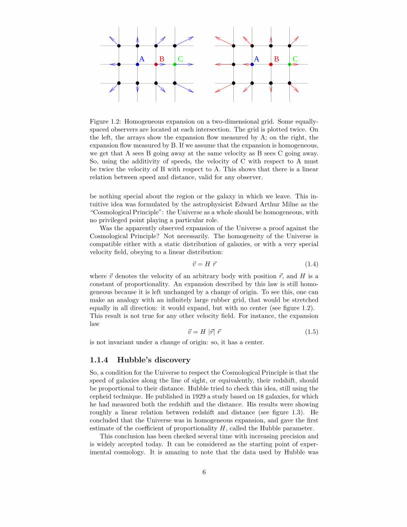
At the beginning of the XX-th century, the understanding of the global structureof the Universe beyond the scale of the solar system was still relying on purespeculation. In 1750, with a remarkable intuition, Thomas Wright noticed thatthe luminous stripe observed in the night sky and called the Milky Way couldbe a consequence of the spatial distribution of stars: they could form a thinplate, what we call now a galaxy. At that time, with the help of telescopes,many faint and diffuse objects had been already observed and listed, under thegeneric name of nebulae - in addition to the Andromeda nebula which is visibleby eye, and has been known many centuries before the invention of telescope.Soon after the proposal of Wright, the philosopher Emmanuel Kant suggestedthat some of these nebulae could be some other clusters of stars, far outsidethe Milky Way. So, the idea of a galactic structure appeared in the mind ofastronomers during the XVIII-th century, but even in the following centurythere was no way to check it on an experimental basis.

At the beginning of the nineteenth century, some physicists observed thefirst spectral lines. In 1842, Johann Christian Doppler argued that if an ob-server receives a wave emitted by a body in motion, the wavelength that he willmeasure will be shifted proportionally to the speed of the emitting body withrespect to the observer (projected along the line of sight):

∆λ/λ = ~v.~n/c (1.1)

where c is the celerity of the wave (See figure 1.1). He suggested that thiseffect could be observable for sound waves, and maybe also for light. The laterassumption was checked experimentally in 1868 by Sir William Huggins, whofound that the spectral lines of some neighboring stars were slightly shiftedtoward the red or blue ends of the spectrum. So, it was possible to know theprojection along the line of sight of star velocities, vr, using

z ≡ ∆λ/λ = vr/c (1.2)

where z is called the redshift (it is negative in case of blue-shift) and c is thespeed of light. Note that the redshift gives no indication concerning the distanceof the star. At the beginning of the XX-th century, with increasingly goodinstruments, people could also measure the redshift of some nebulae. The firstmeasurements, performed on the brightest objects, indicated some arbitrarydistribution of red and blue-shifts, like for stars. Then, with more observations,

4

vn

Figure 1.1: The Doppler effect

it appeared that the statistics was biased in favor of red-shifts, suggesting thata majority of nebulae were going away from us, unlike stars. This was raisingnew questions concerning the distance and the nature of nebulae.

1.1.2 The discovery of the galactic structure

In the 1920’s, Leavitt and Shapley studied some particular stars, called thecepheids, known to have a periodic time-varying luminosity. They could showthat the period of cepheids is proportional to their absolute luminosity L (theabsolute luminosity is the total amount of light emitted by unit of time, i.e., theflux integrated on a closed surface around the star). They were also able to givethe coefficient of proportionality. So, by measuring the apparent luminosity, i.e.the flux l per unit of surface through an instrument pointing to the star, it waseasy to get the distance of the star r from

L = l ×(

4πr2)

. (1.3)

Using this technique, it became possible to measure the distance of variouscepheids inside our galaxies, and to obtain the first estimate of the characteristicsize of the stellar disk of the Milky Way (known today to be around 80.000 light-years).

But what about nebulae? In 1923, the 2.50m telescope of Mount Wilson (LosAngeles) allowed Edwin Hubble to make the first observation of individual starsinside the brightest nebula, Andromeda. Some of these were found to behave likecepheids, leading Hubble to give an estimate of the distance of Andromeda. Hefound approximately 900.000 light-years (but later, when cepheids were knownbetter, this distance was established to be around 2 million light-years). Thatwas the first confirmation of the galactic structure of the Universe: some nebulaewere likely to be some distant replicas of the Milky Way, and the galaxies wereseparated by large voids.

1.1.3 The Cosmological Principle

This observation, together with the fact that most nebulae are redshifted (ex-cepted for some of the nearest ones like Andromeda), was an indication that onthe largest observable scales, the Universe was expanding. At the beginning,this idea was not widely accepted. Indeed, in the most general case, a givendynamics of expansion takes place around a center. Seeing the Universe in ex-pansion around us seemed to be an evidence for the existence of a center in theUniverse, very close to our own galaxy.

Until the middle age, the Cosmos was thought to be organized aroundmankind, but the common wisdom of modern science suggests that there should

5

A AB BC C

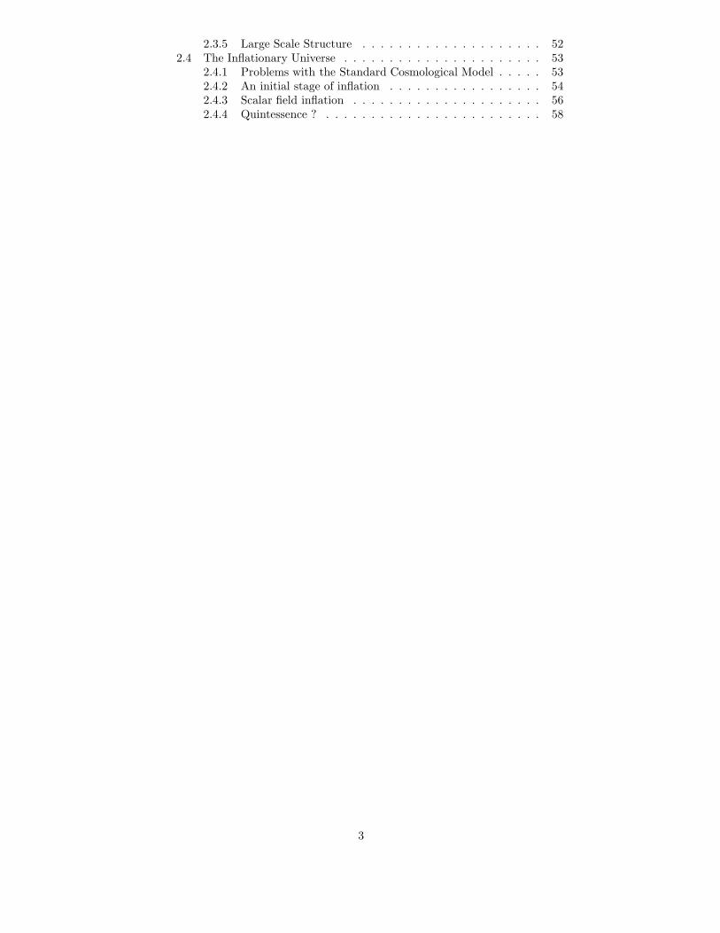
Figure 1.2: Homogeneous expansion on a two-dimensional grid. Some equally-spaced observers are located at each intersection. The grid is plotted twice. Onthe left, the arrays show the expansion flow measured by A; on the right, theexpansion flow measured by B. If we assume that the expansion is homogeneous,we get that A sees B going away at the same velocity as B sees C going away.So, using the additivity of speeds, the velocity of C with respect to A mustbe twice the velocity of B with respect to A. This shows that there is a linearrelation between speed and distance, valid for any observer.

be nothing special about the region or the galaxy in which we leave. This in-tuitive idea was formulated by the astrophysicist Edward Arthur Milne as the“Cosmological Principle”: the Universe as a whole should be homogeneous, withno privileged point playing a particular role.

Was the apparently observed expansion of the Universe a proof against theCosmological Principle? Not necessarily. The homogeneity of the Universe iscompatible either with a static distribution of galaxies, or with a very specialvelocity field, obeying to a linear distribution:

~v = H ~r (1.4)

where ~v denotes the velocity of an arbitrary body with position ~r, and H is aconstant of proportionality. An expansion described by this law is still homo-geneous because it is left unchanged by a change of origin. To see this, one canmake an analogy with an infinitely large rubber grid, that would be stretchedequally in all direction: it would expand, but with no center (see figure 1.2).This result is not true for any other velocity field. For instance, the expansionlaw

~v = H |~r| ~r (1.5)

is not invariant under a change of origin: so, it has a center.

1.1.4 Hubble’s discovery

So, a condition for the Universe to respect the Cosmological Principle is that thespeed of galaxies along the line of sight, or equivalently, their redshift, shouldbe proportional to their distance. Hubble tried to check this idea, still using thecepheid technique. He published in 1929 a study based on 18 galaxies, for whichhe had measured both the redshift and the distance. His results were showingroughly a linear relation between redshift and distance (see figure 1.3). Heconcluded that the Universe was in homogeneous expansion, and gave the firstestimate of the coefficient of proportionality H , called the Hubble parameter.

This conclusion has been checked several time with increasing precision andis widely accepted today. It can be considered as the starting point of exper-imental cosmology. It is amazing to note that the data used by Hubble was

6

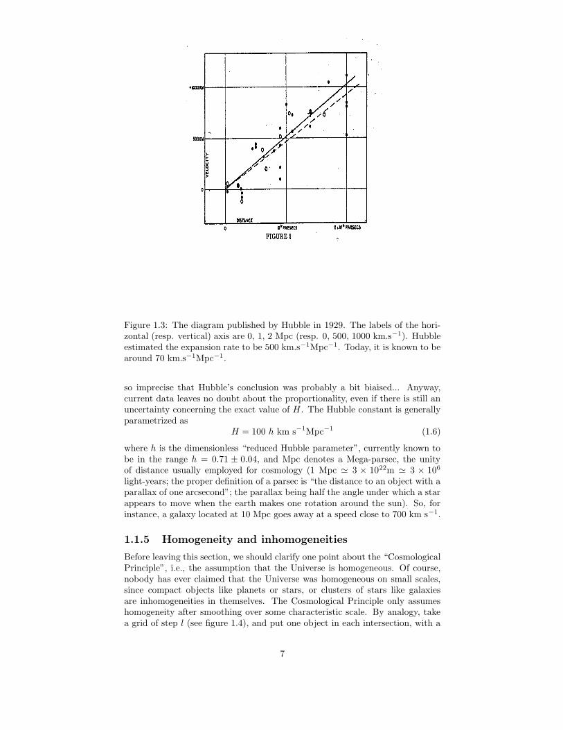
Figure 1.3: The diagram published by Hubble in 1929. The labels of the hori-zontal (resp. vertical) axis are 0, 1, 2 Mpc (resp. 0, 500, 1000 km.s−1). Hubbleestimated the expansion rate to be 500 km.s−1Mpc−1. Today, it is known to bearound 70 km.s−1Mpc−1.

so imprecise that Hubble’s conclusion was probably a bit biaised... Anyway,current data leaves no doubt about the proportionality, even if there is still anuncertainty concerning the exact value of H . The Hubble constant is generallyparametrized as

H = 100 h km s−1Mpc−1 (1.6)

where h is the dimensionless “reduced Hubble parameter”, currently known tobe in the range h = 0.71 ± 0.04, and Mpc denotes a Mega-parsec, the unityof distance usually employed for cosmology (1 Mpc ' 3 × 1022m ' 3 × 106

light-years; the proper definition of a parsec is “the distance to an object with aparallax of one arcsecond”; the parallax being half the angle under which a starappears to move when the earth makes one rotation around the sun). So, forinstance, a galaxy located at 10 Mpc goes away at a speed close to 700 km s−1.

1.1.5 Homogeneity and inhomogeneities

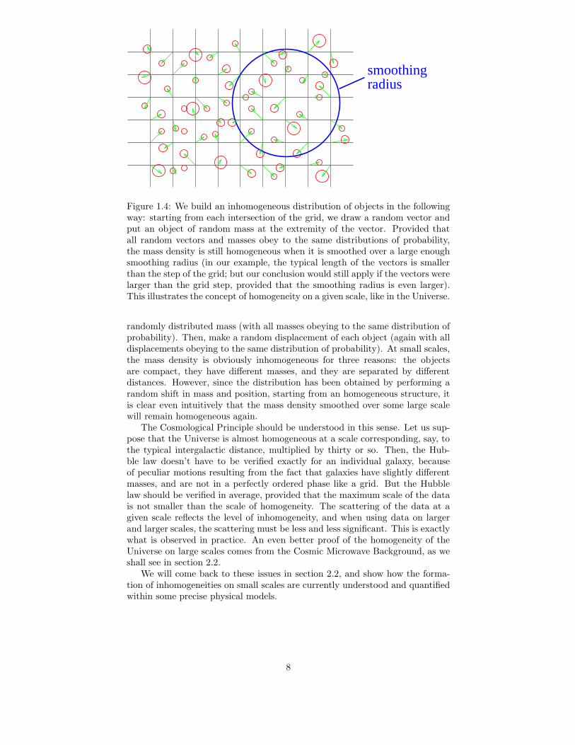
Before leaving this section, we should clarify one point about the “CosmologicalPrinciple”, i.e., the assumption that the Universe is homogeneous. Of course,nobody has ever claimed that the Universe was homogeneous on small scales,since compact objects like planets or stars, or clusters of stars like galaxiesare inhomogeneities in themselves. The Cosmological Principle only assumeshomogeneity after smoothing over some characteristic scale. By analogy, takea grid of step l (see figure 1.4), and put one object in each intersection, with a

7

smoothingradius

Figure 1.4: We build an inhomogeneous distribution of objects in the followingway: starting from each intersection of the grid, we draw a random vector andput an object of random mass at the extremity of the vector. Provided thatall random vectors and masses obey to the same distributions of probability,the mass density is still homogeneous when it is smoothed over a large enoughsmoothing radius (in our example, the typical length of the vectors is smallerthan the step of the grid; but our conclusion would still apply if the vectors werelarger than the grid step, provided that the smoothing radius is even larger).This illustrates the concept of homogeneity on a given scale, like in the Universe.

randomly distributed mass (with all masses obeying to the same distribution ofprobability). Then, make a random displacement of each object (again with alldisplacements obeying to the same distribution of probability). At small scales,the mass density is obviously inhomogeneous for three reasons: the objectsare compact, they have different masses, and they are separated by differentdistances. However, since the distribution has been obtained by performing arandom shift in mass and position, starting from an homogeneous structure, itis clear even intuitively that the mass density smoothed over some large scalewill remain homogeneous again.

The Cosmological Principle should be understood in this sense. Let us sup-pose that the Universe is almost homogeneous at a scale corresponding, say, tothe typical intergalactic distance, multiplied by thirty or so. Then, the Hub-ble law doesn’t have to be verified exactly for an individual galaxy, becauseof peculiar motions resulting from the fact that galaxies have slightly differentmasses, and are not in a perfectly ordered phase like a grid. But the Hubblelaw should be verified in average, provided that the maximum scale of the datais not smaller than the scale of homogeneity. The scattering of the data at agiven scale reflects the level of inhomogeneity, and when using data on largerand larger scales, the scattering must be less and less significant. This is exactlywhat is observed in practice. An even better proof of the homogeneity of theUniverse on large scales comes from the Cosmic Microwave Background, as weshall see in section 2.2.

We will come back to these issues in section 2.2, and show how the forma-tion of inhomogeneities on small scales are currently understood and quantifiedwithin some precise physical models.

8

1.2 The Universe Expansion from Newtonian Grav-

ity

It is not enough to observe the galactic motions, one should also try to explainit with the laws of physics.

1.2.1 Newtonian Gravity versus General Relativity

On cosmic scales, the only force expected to be relevant is gravity. The firsttheory of gravitation, derived by Newton, was embedded later by Einstein intoa more general theory: General Relativity (thereafter denoted GR). However,in simple words, GR is relevant only for describing gravitational forces betweenbodies which have relative motions comparable to the speed of light1. In mostother cases, Newton’s gravity gives a sufficiently accurate description.

Precisely, the speed of neighboring galaxies is always much smaller thanthe speed of light. So, a priori, Newtonian gravity should be able to explainthe Hubble flow. One could even think that historically, Newton’s law led tothe prediction of the Universe expansion, or at least, to its first interpretation.Amazingly, and for reasons which are more mathematical than physical, it hap-pened not to be the case: the first attempts to describe the global dynamicsof the Universe came with GR, in the 1910’s. In this course, for pedagogicalpurposes, we will not follow the historical order, and start with the Newtonianapproach.

Newton himself did the first step in the argumentation. He noticed thatif the Universe was of finite size, and governed by the law of gravity, then allmassive bodies would unavoidably concentrate into a single point, just becauseof gravitational attraction. If instead it was infinite, and with an approximatelyhomogeneous distribution at initial time, it could concentrate into several points,like planets and stars, because there would be no center to fall in. In that case,the motion of each massive body would be driven by the sum of an infinitenumber of gravitational forces. Since the mathematics of that time didn’t allowto deal with this situation, Newton didn’t proceed with his argument.

1.2.2 The rate of expansion from Gauss theorem

In fact, using Gauss theorem, this problem turns out to be quite simple. Supposethat the Universe consists in many massive bodies distributed in an isotropic andhomogeneous way (i.e., for any observer, the distribution looks the same in alldirections). This should be a good modelization of the Universe on sufficientlylarge scales. We wish to compute the motion of a particle located at a distancer away from us. Because the Universe is assumed to be isotropic, the problem isspherically symmetric, and we can employ Gauss theorem on a sphere centeredon us, and of radius r (see figure 1.5). So, the acceleration of any particle onthe surface of the sphere reads

r = −GM(r)

r2(1.7)

where G is Newton’s constant and M(r) is the mass contained inside the sphereof radius r. In other words, the particle feels the same force as if it had atwo-body interaction with the mass of the sphere concentrated at the center.Note that r varies with time, but M(r) remains constant: because of spherical

1Going a little bit more into details, it is also relevant when an object is so heavy and soclose that the speed of liberation from this object - defined like the speed of liberation fromthe Earth - is comparable to the speed of light.

9

O

r

Figure 1.5: Gauss theorem applied to the local Universe.

symmetry, no particles can enter or leave the sphere, which contains always thesame mass.

Since Gauss theorem allows us to make completely abstraction of the massoutside the sphere, we can make an analogy with the motion e.g. of a satelliteejected vertically from the Earth. We know that this motion depends on theinitial velocity, compared with the speed of liberation from the Earth: if theinitial speed is large enough, the satellites goes away indefinitely, otherwise itstops and falls down. We can see this mathematically by multiplying equation(1.7) by r, and integrating it over time:

r2

2=

GM(r)

r− k

2(1.8)

where k is a constant of integration. We can replace the mass M(r) by thevolume of the sphere multiplied by the homogeneous mass density ρmass, andrearrange the equation as

(

r

r

)2

=8πG3

ρmass −k

r2. (1.9)

The quantity r/r is called the rate of expansion. Since M(r) is time-independent,the mass density evolves as ρmass ∝ r−3 (i.e., matter is simply diluted when theUniverse expands). The behavior of r(t) depends on the sign of k. If k is posi-tive, r(t) can grow at early times but it always decreases at late times, like thealtitude of the satellite falling back on Earth: this would correspond to a Uni-verse expanding first, and then collapsing. If k is zero or negative, the expansionlasts forever.

In the case of the satellite, the critical value, which is the speed of liberation(at a given altitude), depends on the mass of the Earth. By analogy, in the caseof the Universe, the important quantity that should be compared with somecritical value is the homogeneous mass density. If at any time, ρmass it is biggerthan the critical value

ρmass =3(r/r)2

8πG (1.10)

then k is positive and the Universe will re-collapse. Physically, what it meansis that the gravitational force wins against inertial effects. In the other case,the Universe expands forever, because the density is too small with respectto the expansion velocity, and gravitation never takes over inertia. The casek = 0 corresponds to a kind of equilibrium between gravitation and inertia.The Universe expands forever, following a power–law: r(t) ∝ t2/3.

10

k>0

k=0

k<0

r

t

Figure 1.6: The motion of expansion in a Newtonian Universe is equivalent tothat of a body ejected from Earth. It depends on the initial rate of expansion,compared with the equivalent of the speed of liberation. When the parameterk is zero or negative, the expansion lasts forever, otherwise the Universe re-collapses (r → 0).

1.2.3 The limitations of Newtonian predictions

In the previous calculation, we cheated a little bit: we assumed that the Universewas isotropic around us, but we didn’t check that it was isotropic everywhere(and therefore homogeneous). Following what we said before, homogeneousexpansion requires proportionality between speed and distance. Looking atequation (1.9), we see immediately that this is true at a given time only when k =0. So, it seems that the other solutions are not compatible with the CosmologicalPrinciple.

This argument shouldn’t be taken seriously, because the link that we madebetween homogeneity and linear expansion was based on the additivity of speed(look for instance at the caption of figure 1.2), and therefore, on Newtonianmechanics. But Newtonian mechanics cannot be applied at large distances,where v becomes large and comparable to the speed of light. This would occurfor a characteristic scale called the Hubble radius RH :

RH = cH−1, (1.11)

at which the Newtonian expansion law gives v = HRH = c.So, the full problem has to be formulated in relativistic terms. In the GR

results, we will see again some solutions with k 6= 0, but they will remaincompatible with the homogeneity of the Universe.

1.3 General relativity and the Friemann-Lemaıtre

model

It is far beyond the scope of this course to introduce General Relativity, and toderive step by step the relativistic laws governing the evolution Universe. Wewill simply write these laws, asking the reader to admit them - and in orderto give a perfume of the underlying physical concepts, we will comment on thedifferences with their Newtonian counterparts.

11

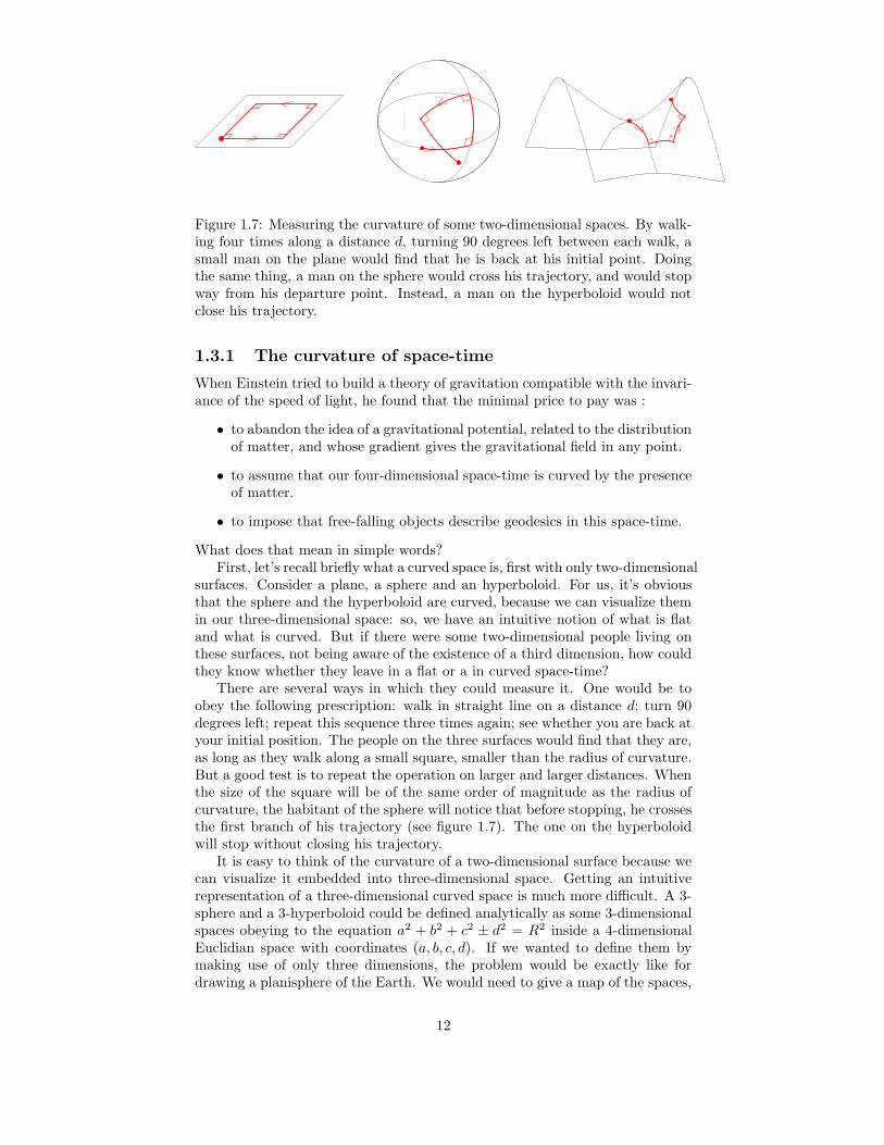
Figure 1.7: Measuring the curvature of some two-dimensional spaces. By walk-ing four times along a distance d, turning 90 degrees left between each walk, asmall man on the plane would find that he is back at his initial point. Doingthe same thing, a man on the sphere would cross his trajectory, and would stopway from his departure point. Instead, a man on the hyperboloid would notclose his trajectory.

1.3.1 The curvature of space-time

When Einstein tried to build a theory of gravitation compatible with the invari-ance of the speed of light, he found that the minimal price to pay was :

• to abandon the idea of a gravitational potential, related to the distributionof matter, and whose gradient gives the gravitational field in any point.

• to assume that our four-dimensional space-time is curved by the presenceof matter.

• to impose that free-falling objects describe geodesics in this space-time.

What does that mean in simple words?First, let’s recall briefly what a curved space is, first with only two-dimensional

surfaces. Consider a plane, a sphere and an hyperboloid. For us, it’s obviousthat the sphere and the hyperboloid are curved, because we can visualize themin our three-dimensional space: so, we have an intuitive notion of what is flatand what is curved. But if there were some two-dimensional people living onthese surfaces, not being aware of the existence of a third dimension, how couldthey know whether they leave in a flat or a in curved space-time?

There are several ways in which they could measure it. One would be toobey the following prescription: walk in straight line on a distance d; turn 90degrees left; repeat this sequence three times again; see whether you are back atyour initial position. The people on the three surfaces would find that they are,as long as they walk along a small square, smaller than the radius of curvature.But a good test is to repeat the operation on larger and larger distances. Whenthe size of the square will be of the same order of magnitude as the radius ofcurvature, the habitant of the sphere will notice that before stopping, he crossesthe first branch of his trajectory (see figure 1.7). The one on the hyperboloidwill stop without closing his trajectory.

It is easy to think of the curvature of a two-dimensional surface because wecan visualize it embedded into three-dimensional space. Getting an intuitiverepresentation of a three-dimensional curved space is much more difficult. A 3-sphere and a 3-hyperboloid could be defined analytically as some 3-dimensionalspaces obeying to the equation a2 + b2 + c2 ± d2 = R2 inside a 4-dimensionalEuclidian space with coordinates (a, b, c, d). If we wanted to define them bymaking use of only three dimensions, the problem would be exactly like fordrawing a planisphere of the Earth. We would need to give a map of the spaces,

12

x

y

C

A

B

Figure 1.8: Gravitational lensing. Somewhere between an object C and a ter-restrial observer A, a massive object B - for instance, a galaxy - curves its sur-rounding space-time. Here, for simplicity, we only draw two spatial dimensions.In absence of gravity and curvature, the only possible trajectory of light betweenC and A would be a straight line. But because of curvature, the straight lineis not anymore the shortest trajectory. Photons prefer to follow two geodesics,symmetrical around B. So, the observer will not see one image of C, but twodistinct images. In fact, if we restore the third spatial dimension, and if thethree points are perfectly aligned, the image of C will appear as a ring aroundB. This phenomenon is observed in practice.

together with a crucial information: the scale of the map as a function of thelocation on the map - the scale on a planisphere is not uniform! This wouldbring us to a mathematical formalism, called Riemann geometry, that we don’thave time to introduce here.

That was still four three dimensions. Finally, the curvature of a four-dimensional space-time is impossible to visualize intuitively, first because it haseven more dimensions, and second because even in special/general relativity,there is a difference between time and space (for the readers who are familiarwith special relativity, what is referred here is the negative signature of themetric).

The Einstein theory of gravitation says that four-dimensional space-time iscurved, and that the curvature in each point is given entirely in terms of thematter content in this point. In simple words, this means that the curvatureplays more or less the same role as the potential in Newtonian gravity. But thepotential was simply a function of space and time coordinates. In GR, the fullcurvature is described not by a function, but by something more complicated -like a matrix of functions obeying to particular laws - called a tensor.

Finally, the definition of geodesics (the trajectories of free-falling bodies)is the following. Take an initial point and an initial direction. They define aunique line, called a geodesic, such that any segment of the line gives the shortesttrajectory between the two points (so, for instance, on a sphere of radius R,the geodesics are all the great circles of radius R, and nothing else). Of course,geodesics depend on curvature. All free-falling bodies follow geodesics, includinglight rays. This leads for instance to the phenomenon of gravitational lensing(see figure 1.8).

So, in General Relativity, gravitation is not formulated as a force or a field,but as a curvature of space-time, sourced by matter. All isolated systems followgeodesics which are bent by the curvature. In this way, their trajectories are

13

affected by the distribution of matter around them: this is precisely what gravitymeans.

1.3.2 Building the first cosmological models

After obtaining the mathematical formulation of General Relativity, around1916, Einstein studied various testable consequences of his theory in the solarsystem (e.g., corrections to the trajectory of Mercury, or to the apparent diam-eter of the sun during an eclipse). But remarkably, he immediately understoodthat GR could also be applied to the Universe as a whole, and published somefirst attempts in 1917. However, Hubble’s results concerning the expansionwere not known at that time, and most physicists had the prejudice that theUniverse should be not only isotropic and homogeneous, but also static – orstationary. As a consequence, Einstein (and other people like De Sitter) foundsome interesting cosmological solutions, but not the ones that really describeour Universe.

A few years later, some other physicists tried to relax the assumption of sta-tionarity. The first was the russo-american Friedmann (in 1922), followed closelyby the Belgian physicist and priest Lemaıtre (in 1927), and then by some amer-icans, Robertson and Walker. When the Hubble flow was discovered in 1929, itbecame clear for a fraction of the scientific community that the Universe couldbe described by the equations of Friedmann, Lemaıtre, Roberston and Walker.However, many people – including Hubble and Einstein himself – remained re-luctant to this idea for many years. Today, the Friedmann – Lemaıtre model isconsidered as one of the major achievements of the XXth century.

Before giving these equations, we should stress that they look pretty muchthe same as the Newtonian results given above - although some terms seemto be identical, but have a different physical interpretation. This similaritywas noticed only much later. Physically, it has to do with the fact that thereexists a generalization of Gauss theorem to GR, known as Birkhoff theorem.So, as in Newtonian gravity, one can study the expansion of the homogeneousUniverse by considering only matter inside an sphere. But in small regions,General Relativity admits Newtonian gravity as an asymptotic limit, and so theequations have many similarities.

1.3.3 Our Universe is curved

The Friemann-Lemaıtre model is defined as the most general solution of the lawsof General Relativity, assuming that the Universe is isotropic and homogeneous.We have seen that in GR, matter curves space-time. So, the Universe is curvedby its own matter content, along its four space and time dimensions. However,because we assume homogeneity, we can decompose the total curvature into twoparts:

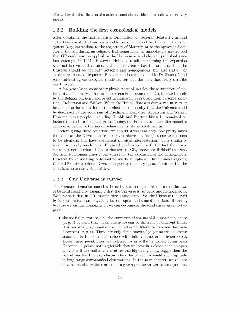
• the spatial curvature, i.e., the curvature of the usual 3-dimensional space(x, y, z) at fixed time. This curvature can be different at different times.It is maximally symmetric, i.e., it makes no difference between the threedirections (x, y, z). There are only three maximally symmetric solutions:space can be Euclidean, a 3-sphere with finite volume, or a 3-hyperboloid.These three possibilities are referred to as a flat, a closed or an openUniverse. A priori, nothing forbids that we leave in a closed or in an openUniverse: if the radius of curvature was big enough, say, bigger than thesize of our local galaxy cluster, then the curvature would show up onlyin long range astronomical observations. In the next chapter, we will seehow recent observations are able to give a precise answer to this question.

14

• the two-dimensional space-time curvature, i.e., for instance, the curvatureof the (t, x) space-time. Because of isotropy, the curvature of the (t, y)and the (t, z) space-time have to be the same. This curvature is the oneresponsible for the expansion. Together with the spatial curvature, it fullydescribes gravity in the homogeneous Universe.

The second part is a little bit more difficult to understand for the reader whois not familiar with GR, and causes a big cultural change in one’s intuitiveunderstanding of space and time.

1.3.4 Comoving coordinates

In the spirit of General Relativity, we will consider a set of three variables thatwill represent the spatial coordinates (i.e., a way of mapping space, and of givinga label to each point), but NOT directly a measure of distance!

The laws of GR allow us to work with any system of coordinates that weprefer. For simplicity, in the Friedmann model, people generally employ a par-ticular system of spherical coordinates (r, θ, φ) called “comoving coordinates”,with the following striking property: the physical distance dl between two in-finitesimally close objects with coordinates (r, θ, φ) and (r + dr, θ + dθ, z + dz)is not given by

dl2 = dr2 + r2(dθ2 + sin2θ dφ2) (1.12)

as in usual Euclidean space, but

dl2 = a2(t)

[

dr2

1 − kr2+ r2(dθ2 + sin2θ dφ2)

]

(1.13)

where a(t) is a function of time, called the scale factor, whose time-variationsaccount for the curvature of two-dimensional space-time; and k is a constantnumber, related to the spatial curvature: if k = 0, the Universe is flat, if k > 0,it is closed, and if k < 0, it is open. In the last two cases, the radius of curvatureRc is given by

Rc(t) =a(t)√

|k|. (1.14)

When the Universe is closed, it has a finite volume, so the coordinate r is definedonly up to a finite value: 0 ≤ r < 1/

√k.

If k was equal to zero and a was constant in time, we could redefine thecoordinate system with (r′, θ′, φ′) = (ar, θ, φ), find the usual expression (1.12)for distances, and go back to Newtonian mechanics. So, we stress again thatthe curvature really manifests itself as k 6= 0 (for spatial curvature) and a 6= 0(for the remaining space-time curvature).

Note that when k = 0, we can rewrite dl2 in Cartesian coordinates:

dl2 = a2(t)(

dx2 + dy2 + dz2)

. (1.15)

In that case, the expressions for dl contains only the differentials dx, dy, dz,and is obviously left unchanged by a change of origin - as it should be, becausewe assume a homogeneous Universe. But when k 6= 0, there is the additionalfactor 1/(1 − kr2), where r is the distance to the origin. So, naively, one couldthink that we are breaking the homogeneity of the Universe, and privileginga particular point. This would be true in Euclidean geometry, but in curvedgeometry, it is only an artifact. Indeed, choosing a system of coordinates isequivalent to mapping a curved surface on a plane. By analogy, if one draws aplanisphere of half-of-the-Earth by projecting onto a plane, one has to chose aparticular point defining the axis of the projection. Then, the scale of the map

15

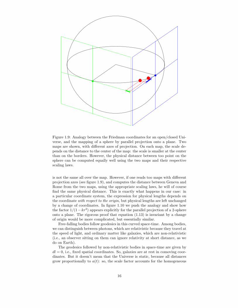
Figure 1.9: Analogy between the Friedman coordinates for an open/closed Uni-verse, and the mapping of a sphere by parallel projection onto a plane. Twomaps are shown, with different axes of projection. On each map, the scale de-pends on the distance to the center of the map: the scale is smaller at the centerthan on the borders. However, the physical distance between too point on thesphere can be computed equally well using the two maps and their respectivescaling laws.

is not the same all over the map. However, if one reads too maps with differentprojection axes (see figure 1.9), and computes the distance between Geneva andRome from the two maps, using the appropriate scaling laws, he will of coursefind the same physical distance. This is exactly what happens in our case: ina particular coordinate system, the expression for physical lengths depends onthe coordinate with respect to the origin, but physical lengths are left unchangedby a change of coordinates. In figure 1.10 we push the analogy and show howthe factor 1/(1−kr2) appears explicitly for the parallel projection of a 2-sphereonto a plane. The rigorous proof that equation (1.13) is invariant by a changeof origin would be more complicated, but essentially similar.

Free-falling bodies follow geodesics in this curved space-time. Among bodies,we can distinguish between photons, which are relativistic because they travel atthe speed of light, and ordinary matter like galaxies, which are non-relativistic(i.e., an observer sitting on them can ignore relativity at short distance, as wedo on Earth).

The geodesics followed by non-relativistic bodies in space-time are given bydl = 0, i.e., fixed spatial coordinates. So, galaxies are at rest in comoving coor-dinates. But it doesn’t mean that the Universe is static, because all distancesgrow proportionally to a(t): so, the scale factor accounts for the homogeneous

16

0

r

θR

dl dr

Figure 1.10: We push the analogy between the Friedmann coordinates in a closedUniverse, and the parallel projection of a half–sphere onto a plane. The physicaldistance dl on the surface of the sphere corresponds to the coordinate interval

dr, such that dl = dr/cos θ = dr/√

1 − sin2θ = dr/√

1 − (r/R)2, where R isthe radius of the sphere. This is exactly the same law as in a closed FriedmanUniverse.

expansion. A simple analogy helps in understanding this subtle concept. Letus take a rubber balloon and draw some points on the surface. Then, we inflatethe balloon. The distances between all the points grow proportionally to theradius of the balloon. This is not because the points have a proper motion onthe surface, but because all the lengths on the surface of the balloon increasewith time.

The geodesics followed by photons are straight lines in 3-space, but not inspace-time. Locally, they obey to the same relation as in Newtonian mechanics:c dt = dl, i.e.,

c2dt2 = a2(t)

[

dr2

1 − kr2+ r2(dθ2 + sin2θ dφ2)

]

. (1.16)

So, on large scales, the distance traveled by light in a given time interval isnot ∆l = c∆t like in Newtonian mechanics, but is given by integrating the in-finitesimal equation of motion. We can write this integral, taking for simplicitya photon with constant (θ, φ) coordinates (i.e., the origin is chosen on the tra-jectory of the photon). Between t1 and t2, the change in comoving coordinates

for such a photon is given by

∫ r2

r1

dr√1 − kr2

=

∫ t2

t1

c

a(t)dt. (1.17)

This propagation equation of light is extremely important - probably, one ofthe two most important of cosmology, together with the Friedmann equation,that we will give soon. It is with this equation that we are able today to measurethe curvature of the Universe, its age, its acceleration, and other fundamentalquantities.

1.3.5 Bending of light in the expanding Universe

Lets give a few examples of the implications of equation (1.16), which give thebending of the trajectories followed by photons in our curved space-time, asillustrated in figure 1.11.

17

rre

to

te eθ

Figure 1.11: An illustration of the propagation of photons in our Universe. Thedimensions shown here are (t, r, θ): we skip φ for the purpose of representa-tion. We are siting at the origin, and at a time t0, we can see a the light ofa galaxy emitted at (te, re, θe). Before reaching us, the light from this galaxyhas traveled over a curved trajectory. In any point, the slope dr/dt is givenby equation (1.16). So, the relation between re and (t0 − te) depends on thespatial curvature and on the scale factor evolution. The trajectory would be astraight line in space-time only if k = 0 and a = constant, i.e., in the limit ofNewtonian mechanics in Euclidean space. The ensemble of all possible photontrajectories crossing r = 0 at t = t0 is called our “past light cone”, visible herein orange. Asymptotically, near the origin, it can be approximated by a linearcone with dl = cdt, showing that at small distance, the physics is approximatelyNewtonian.

The redshift.First, a simple calculation based on equation (1.16) - we don’t include it here

- gives the redshift associated with a given source of light. Take two observerssitting on two galaxies (with fixed comoving coordinates). A light signal is sentfrom one observer to the other. At the time of emission t1, the first observermeasures the wavelength λ1. At the time of reception t2, the second observerwill measure the wavelength λ2 such that

z =δλ

λ=

λ2 − λ1

λ1=

a(t2)

a(t1)− 1 . (1.18)

So, the redshift depends on the variation of the scale-factor between the timeof emission and reception, but not on the curvature parameter k. This canbe understood as if the scale-factor represented the “stretching” of light in out

18

curved space-time. We can check that when the Universe expands (a(t2) >a(t1)), the wavelengths are enhanced (λ2 > λ1), and the spectral lines arered-shifted (contraction would lead to blue-shift, i.e., to a negative redshiftparameter z < 0).

In real life, what we see when we observe the sky is never directly the dis-tance, size, or velocity of an object, but the light traveling from it. So, by study-ing spectral lines, we can easily measure the redshifts. This is why astronomers,when they refer to an object or to an event in the Universe, generally mentionthe redshift rather than the distance or the time. It’s only when the functiona(t) is known - and as we will see later, we almost know it in our Universe -that a given redshift can be related to a given time and distance.

The importance of the redshift as a measure of time and distance comesfrom the fact that we don’t see our full space-time, but only our past line-cone, i.e., a three-dimensional subspace of the full four-dimensional space-time,corresponding to all points which could emit a light signal that we would receivetoday on Earth. If we remove the coordinate φ and draw the past line-coneof a given observer, it does look like a cone, of course curved like all photontrajectories (see figure 1.11).

Also note that in Newtonian mechanics, the redshift was defined as z = v/c,and seemed to be limited to |z| < 1. The true GR expression doesn’t have suchlimitations, since the ratio of the scale factors can be arbitrarily large withoutviolating any fundamental principle. And indeed, observations do show manyobjects - like quasars - at redshifts of 2 or even bigger. We’ll see later that wealso observe the Cosmic Microwave Background at a redshift of approximatelyz = 1000!

The Hubble parameter in General Relativity.In the limit of small redshift, we expect to recover the Newtonian results,

and to find a relation similar to z = v/c = Hr/c. To show this, let’s assumethat t0 is the present time, and that our galaxy is at r = 0. We want to computethe redshift of a nearby galaxy, which emitted the light that we receive todayat a time t0 − dt. In the limit of small dt, the equation of propagation of lightshows the physical distance between the galaxy and us is simply

dl = c dt (1.19)

while the redshift of the galaxy is

z =a(t0)

a(t0 − dt)− 1 =

1

1 − a(t0)a(t0)dt

− 1 =a(t0)

a(t0)dt . (1.20)

By combining these two relations we obtain

z =a(t0)

a(t0)

dl

c. (1.21)

So, at small redshift, we recover the Hubble law, and the role of the Hubbleparameter is played by a(t0)/a(t0). In the Friedmann Universe, we will directlydefine the Hubble parameter as the expansion rate of the scale factor:

H(t) =a(t)

a(t). (1.22)

The present value of H is generally noted H0:

H0 = 100h km s−1Mpc−1, 0.5 < h < 0.8. (1.23)

19

Angular diameter – redshift relation.When looking at the sky, we don’t see directly the size of the objects, but

only their angular diameter. In Euclidean space, i.e. in absence of gravity, theangular diameter dθ of an object would be related to its size dl and distance rthrough

dθ =dl

r. (1.24)

Recalling that z = v/c and v = Hr, we easily find an angular diameter – redshiftrelation valid in Euclidean space:

dθ =H dl

c z. (1.25)

In General Relativity, because of the bending of light by gravity, the steps of thecalculation are different. Using the definition of infinitesimal distances (1.13),we see that the physical size dl of an object is related to its angular diameterdθ through

dl = a(te) re dθ (1.26)

where te is the time at which the galaxy emitted the light ray that we observetoday on Earth, and re is the comoving coordinate of the object. The equationof motion of light gives a relation between re and te:

∫ 0

re

−dr√1− kr2

=

∫ t0

te

c

a(t)dt (1.27)

where t0 is the time today. So, the relation between re and te depends on a(t)and k.

If we knew the function a(t) and the value of k, we could calculate theintegral (1.27) and re-express equation (1.26) in the form

dθ =H dl

c zf(z) (1.28)

where f(z) would be a function of redshift, accounting for general relativisticcorrections, and depending on the curvature. We conclude that in the Fried-mann Universe, for an object of fixed size and redshift, the angular diameterdepends on the curvature - as illustrated graphically in figure 1.12. Therefore,if we know in advance the physical size of an object, we can simply measureits redshift, its angular diameter, and immediately obtain some informations onthe geometry of the Universe.

It seems very difficult to know in advance the physical size of a remote object.However, we will see in the next chapter that some beautiful developments ofmodern cosmology enabled physicists to know the physical size of some objectsvisible at a redshift of z ' 1000 (namely, the anisotropies of the CosmologicalMicrowave Background). So, the angular diameter – redshift relation has beenused in the past decade in order to measure the spatial curvature of the Universe.We will show the results in the last section of chapter two.

Apparent Luminosity – redshift relation.We have seen that in Newtonian mechanics, the absolute luminosity of an

object and the apparent luminosity l that we measure on Earth per unit ofsurface are related by

l =L

4πr2=

LH2

4πc2z2. (1.29)

So, if for some reason we know independently the absolute luminosity of acelestial body (like for cepheids), and we measure its redshift, we can obtain thevalue of H , as Hubble did in 1929.

20

’’

dl

r

to

te

re eθeθ

re

Figure 1.12: Angular diameter – redshift relation. We consider an object of fixedsize dl and fixed redshift, sending a light signal at time te that we receive atpresent time t0. All photons travel by definition with θ =constant. However, thebending of their trajectories in the (t, r) plane depends on the spatial curvatureand on the scale factor evolution. So, for fixed te, the comoving coordinate ofthe object, re, depends on curvature. The red lines are supposed to illustratethe trajectory of light in a flat Universe with k = 0. If we keep dl, a(t) andte fixed, but choose a positive value k > 0, we know from equation (1.27) thatthe new coordinate re

′ has to be smaller. But dl is fixed, so the new angledθ′ has to be bigger, as easily seen on the figure for the purple lines. So, in aclosed Universe, objects are seen under a larger angle. Conversely, in an openUniverse, they are seen under a smaller angle.

But we would like to extend this technique to very distant objects (in par-ticular, supernovae, that are observed up to a redshift of two, and are thoughtto have a calibrated absolute luminosity, like cepheids). So, one needs to recom-pute this relation in the framework of general relativity. Because of the bendingof light rays, the trajectory of the photons traveling from an object located ata given redshift depends both on the curvature and the scale factor. So, today,the light will be dispersed on a sphere of variable size.

If we know several objects with the same absolute magnitude, and we plotthem on an apparent magnitude - redshift diagram, we will get a curve whoseshape at small redshift is given by (1.29), and at large redshift by GeneralRelativity corrections (depending on the spatial curvature and the scale factor.)We will see in the next chapter that such an experiment has been performed forsupernovae, leading to one of the most intriguing discovery of the past years.

21

In summary of this section, according to General Relativity, the homoge-neous Universe is curved by its own matter content, and the curvature can bespecified with just one number and one function: the curvature k, and the scalefactor a(t). We should be able to relate these two quantities with what causesthe curvature: the matter density.

1.3.6 The Friedmann law

The Friedmann law relates the scale factor a(t), the spatial curvature parameterk and the homogeneous energy density of the Universe ρ(t):

(

a

a

)2

=8πG3

ρ

c2− kc2

a2. (1.30)

Together with the propagation of light equation, this law is the key ingredientof the Friedmann-Lemaıtre model.

In special/general relativity, the total energy of a particle is the sum of itsrest energy E0 = mc2 plus its momentum energy. So, if we consider only non-relativistic particles like those forming galaxies, we get ρ = ρmassc

2. Then,the Friedmann equation looks exactly like the Newtonian expansion law (1.9),excepted that the function r(t) (representing previously the position of materialpoints) is replaced by the scale factor a(t). Of course, the equations look thesame, but are not equivalent . First, we have already seen that only at verysmall distance, the distinction between the scale factor a(t) and the classicalposition r(t) is irrelevant; on large distances – like the Hubble radius – thedifference of interpretation between the two is crucial. Second, we have seenthat the term proportional to k seems to break the homogeneity of the Universein the Newtonian formalism, while in General Relativity, when it is correctlyinterpreted as the spatial curvature term, it is perfectly consistent with theCosmological Principle.

Actually, there is a third crucial difference between the Friedmann law andthe Newtonian expansion law. In the previous paragraph, we only considerednon-relativistic matter like galaxies. But the Universe also contains relativisticparticles traveling at the speed of light, like photons (and also neutrinos if theirmass is very small). A priori, their gravitational effect on the Universe expansioncould be important. How can we include them?

1.3.7 Relativistic matter and Cosmological constant

The Friedmann equation is true for any types of matter, relativistic or non-relativistic; if there are different species, the total energy density ρ is the sumover the density of all species.

What depends on the type of matter is the relation between ρ and a, i.e.,the way in which energy gets diluted by the expansion.

For non-relativistic matter, the answer is obvious. Take a distribution ofparticles with fixed comoving coordinates. Their energy density equals theirmass density times c2. Look only at the matter contained into a comovingsphere centered around the origin, of comoving radius r. If the sphere is smallwith respect to the curvature, the physical volume inside the sphere is just V =4π3 (a(t)r)3. Since both the sphere and the matter particles have fixed comoving

coordinates, no matter can enter or leave from inside the sphere during theexpansion. Therefore, the mass (or the energy) inside the sphere is conserved.We conclude that ρV is constant and that ρ ∝ a−3.

22

For ultra–relativistic matter like photons, the energy is not given by the restmass but by the frequency ν or the wavelength λ:

E = hν = hc/λ. (1.31)

But we knows that physical wavelengths are stretched proportionally to thescale factor a(t). So, if we repeat the argument of the sphere, assuming nowthat it contains a homogeneous bath of photons with equal wavelength, wesee that the total energy inside the sphere evolves proportionally to a−1. So,the energy density of relativistic matter is proportional to ρ ∝ a−4. If thescale factor increases, the photon energy density decreases faster than that ofordinary matter.

This result could be obtained differently. For any gas of particles with adistribution of velocities, one can define a pressure (corresponding physically tothe shock of particles against the borders if the gas was enclosed into a box).This can be extended to a gas of relativistic particles, for which the speed equalsthe speed of light. A calculation based on statistical mechanics gives the famousresult that the pressure of a relativistic gas is related to its density by p = ρ/3.

In the case of the Friedmann universe, General Relativity provides severalequations: the Friedmann law, and also, for each specie, the equation of conser-vation:

ρ = −3a

a(ρ + p) . (1.32)

This is consistent with what we already said. For non-relativistic matter, likegalaxies, the pressure is negligible (like in a gas of still particles), and we get

ρ = −3a

aρ ⇒ ρ ∝ a−3. (1.33)

For relativistic matter like photons, we get

ρ = −3a

a(1 +

1

3)ρ = −4

a

aρ ⇒ ρ ∝ a−4. (1.34)

Finally, in quantum field theory, it is well–known that the vacuum can have anenergy density different from zero. The Universe could also contain this typeof energy (which can be related to particle physics, phase transitions and spon-taneous symmetry breaking). For vacuum, one can show that p = −ρ. Thismeans that the vacuum energy is never diluted and remains constant. This con-stant energy density was called by Einstein – who introduced it in a completelydifferent way and with other motivations – the Cosmological Constant. We willsee that this term is probably important in our Universe.

23

Chapter 2

The Standard Cosmological

Model

The real Universe is not homogeneous: it contains stars, galaxies, clusters ofgalaxies...

In cosmology, all quantities – like the density and pressure of each specie –are decomposed into a spatial average, called the background, plus some inho-mogeneities. The later are assumed to be small with respect to the backgroundin the early Universe: so, they can be treated like linear perturbations. As aconsequence, the evolution of each Fourier mode is independent of the others.During the evolution, if the perturbations of a given quantity become large, thelinear approximation breaks down, and one has to employ a full non–linear de-scription, which is very complicated in practice. However, for many purposes incosmology, the linear theory is sufficient in order to make testable predictions.

In section 2.1, we will describe the evolution of the homogeneous background.Section 2.2 will give some hints about the evolution of linear perturbations –and also, very briefly, about the final non-linear evolution of matter perturba-tions. Altogether, these two sections provide a brief summary of what is calledthe standard cosmological model, which depends on a few free parameters. Insection 2.3, we will show that the main cosmological parameters have alreadybeen measured with quite good precision. Finally, in section 2.4, we will in-troduce the theory of inflation, which provides some initial conditions both forthe background and for the perturbations in the very early Universe. We willconclude with a few words on the so-called quintessence models.

2.1 The Hot Big Bang scenario

A priori, we don’t know what type of fluid or particles gives the dominantcontributions to the energy density of the Universe. According to the Friedmannequation, this question is related to many fundamental issues, like the behaviorof the scale factor, the spatial curvature, or the past and future evolution of theUniverse...

2.1.1 Various possible scenarios for the history of the Uni-

verse

We will classify the various types of matter that could fill the Universe accordingto their pressure-to-density ratio. The three most likely possibilities are:

24

1. ultra–relativistic particles, with v = c, p = ρ/3, ρ ∝ a−4. Thisincludes photons, massless neutrinos, and eventually other particles thatwould have a very small mass and would be traveling at the speed oflight. The generic name for this kind of matter, which propagates likeelectromagnetic radiation, is precisely “radiation”.

2. non-relativistic pressureless matter – in general, simply called “matter”by opposition to radiation – with v c, p ' 0, ρ ∝ a−3. This appliesessentially to all structures in the Universe: planets, stars, clouds of gas,or galaxies seen as a whole.

3. a possible cosmological constant, with time–invariant energy density andp = −ρ, that might be related to the vacuum of the theory describingelementary particles, or to something more mysterious. Whatever it is, weleave such a constant term as an open possibility. Following the definitiongiven by Einstein, what is actually called the “cosmological constant” Λis not the energy density ρΛ, but the quantity

Λ = 8πGρΛ/c2 (2.1)

which has the dimension of the inverse square of a time.

We write the Friedmann equation including these three terms:

H2 =

(

a

a

)2

=8πG3c2

ρR +8πG3c2

ρM − kc2

a2+

Λ

3(2.2)

where ρR is the radiation density and ρM the matter density. The order inwhich we wrote the four terms on the right–hand side – radiation, matter,spatial curvature, cosmological constant – is not arbitrary. Indeed, they evolvewith respect to the scale factor as a−4, a−3, a−2 and a0. So, if the scale factorskeeps growing, and if these four terms are present in the Universe, there is achance that they all dominate the expansion of the Universe one after each other(see figure 2.1). Of course, it is also possible that some of these terms do notexist at all, or are simply negligible. For instance, some possible scenarios wouldbe:

• only matter domination, from the initial singularity until today (we’ll comeback to the notion of Big Bang later).

• radiation domination → matter domination today.

• radiation dom. → matter dom. → curvature dom. today

• radiation dom. → matter dom. → cosmological constant dom. today

But all the cases that do not respect the order (like for instance: curvaturedomination → matter domination) are impossible.

During each stage, one component strongly dominates the others, and thebehavior of the scale factor, of the Hubble parameter and of the Hubble radiusare given by:

1. Radiation domination:

a2

a2∝ a−4, a(t) ∝ t1/2, H(t) =

1

2t, RH(t) = 2ct. (2.3)

So, the Universe is in decelerated power–law expansion.

25

a

a

a

−4

−3

cst−2

a

H2

Figure 2.1: Evolution of the square of the Hubble parameter, in a scenario inwhich all typical contributions to the Universe expansion (radiation, matter,curvature, cosmological constant) dominate one after each other.

2. Matter domination:

a2

a2∝ a−3, a(t) ∝ t2/3, H(t) =

2

3t, RH(t) =

3

2ct. (2.4)

Again, the Universe is in power–law expansion, but it decelerates moreslowly than during radiation domination.

3. Negative curvature domination (k < 0):

a2

a2∝ a−2, a(t) ∝ t, H(t) =

1

t, RH(t) = ct. (2.5)

An open Universe dominated by its curvature is in linear expansion.

4. Positive curvature domination: if k > 0, and if there is no cosmologicalconstant, the right–hand side finally goes to zero: expansion stops. After,the scale factor starts to decrease. H is negative, but the right–hand sideof the Friedmann equation remains positive. The Universe recollapses. Weknow that we are not in such a phase, because we observe the Universeexpansion. But a priori, we might be living in a closed Universe, slightlybefore the expansion stops.

5. Cosmological constant domination:

a2

a2→ constant, a(t) ∝ exp(Λt/3), H = c/RH =

√

Λ/3. (2.6)

The Universe ends up in exponentially accelerated expansion.

So, in all cases, there seems to be a time in the past at which the scale factorgoes to zero, called the initial singularity or the “Big Bang”. The Friedmanndescription of the Universe is not supposed to hold until a(t) = 0. At some time,when the density reaches a critical value called the Planck density, we believe

26

that gravity has to be described by a quantum theory, where the classical notionof time and space disappears. Proposals for such theories exist, called “stringtheories”. Sometimes, they try to address the initial singularity problem, and tobuild various scenarios for the origin of the Universe. Anyway, this field is stillvery speculative, and of course, our understanding of the origin of the Universewill always break down at some point. A reasonable goal is just to go back asfar as possible, on the basis of testable theories.

The future evolution of the Universe heavily depends on the existence of acosmological constant. If the later is exactly zero, then the future evolutionis dictated by the curvature (if k > 0, the Universe will end up with a “BigCrunch”, where quantum gravity will show up again, and if k ≤ 0 there will beeternal decelerated expansion). If instead there is a positive cosmological term,then the Universe necessarily ends up in eternal accelerated expansion.

2.1.2 The matter budget today

In order to know the past and future evolution of the Universe, it would beenough to measure the present density of radiation, matter and Λ, and also tomeasure H0. Then, thanks to the Friedmann equation, it would be possible toextrapolate a(t) at any time. Let us express this idea mathematically. We takethe Friedmann equation, evaluated today, and divide it by H2

0 :

1 =8πG

3H20 c2

(ρR0 + ρM0) −kc2

a20H

20

+Λ

3H20

. (2.7)

where the subscript 0 means “evaluated today”. Since by construction, thesum of these four terms is one, they represent the relative contributions to thepresent Universe expansion. These terms are usually noted

ΩR =8πG

3H20 c2

ρR0, (2.8)

ΩM =8πG

3H20 c2

ρM0, (2.9)

Ωk =kc2

a20H

20

, (2.10)

ΩΛ =Λ

3H20

, (2.11)

(2.12)

and the “matter budget” equation is

ΩR + ΩM − Ωk + ΩΛ = 1. (2.13)

The Universe is flat provided that

Ω0 ≡ ΩR + ΩM + ΩΛ (2.14)

is equal to one. In that case, as we already know, the total density of matter,radiation and Λ is equal at any time to the critical density

ρc(t) =3c2H2(t)

8πG . (2.15)

Note that the parameters Ωx, where x ∈ R, M, Λ, could have been defined asthe present density of each specie divided by the present critical density:

Ωx =ρx0

ρc0. (2.16)

27

So far, we conclude that the evolution of the Friedmann Universe can be de-scribed entirely in terms of four parameters, called the “cosmological parame-ters”:

ΩR, ΩM, ΩΛ, H0. (2.17)

One of the main purposes of cosmology is to measure the value of the cosmo-logical parameters.

2.1.3 The Cold and Hot Big Bang alternatives

Curiously, after the discovery of the Hubble expansion and of the Friedmannlaw, there were no rapid progresses in cosmology for a few decades. The mostlikely explanation is that most physicists were not considering seriously thepossibility of studying the Universe in the far past, near the initial singularity,because they thought that it would always be impossible to test experimentallyany model of this type.

Nevertheless, a few pioneers tried to think about the origin of the Universe.At the beginning, for simplicity, they assumed that the expansion of the Uni-verse is always dominated by a single component, the one forming galaxies, i.e.,pressureless matter. Since going back in time, the density of matter increasesas a−3, matter had to be very dense at early times. This was formulated as the“Cold Big Bang” scenario.

According to Cold Big Bang, in the early Universe, the density is so highthat matter has to consist in a gas of nucleons and electrons. Then, when thedensity falls below a critical value, some nuclear reactions form the first nuclei -this era is called nucleosynthesis. But later, due to the expansion, the dilution ofmatter is such that nuclear reactions are suppressed (in general, the expansionfreezes out all processes when their characteristic time–scale becomes smallerthan the so–called Hubble time–scale H−1). So, only the lightest nuclei havetime to form in a significant amount. After nucleosynthesis, matter consists in agas of nuclei and electrons, with electromagnetic interactions. When the densitybecomes even smaller, they finally combine into atoms – this second transitionis called the recombination. At late time, any small density inhomogeneityin the gas of atoms is enhanced by gravitational interactions. The atoms getaccumulated into clumps like stars and planets - but this is a different story.

In the middle of the XX-th century, a few particle physicists tried to buildthe first models of nucleosynthesis – the era of nuclei formation. In particular,four groups – each of them not being aware of the work of the others – reachedapproximately the same negative conclusion: in the Cold Big Bang scenario,nucleosynthesis does not work properly, because the formation of hydrogen isstrongly suppressed with respect to that of heavier elements. But this conclusionis at odds with observations: using spectrometry, astronomers know that thereis a lot of hydrogen in stars and clouds of gas. The groups of the Russo-American Gamow in the 1940’s, of the Russian Zel’dovitch (1964), of the BritishHoyle and Tayler (1964), and of Peebles in Princeton (1965) all reached thisconclusion. They also proposed a possible way to reconcile nucleosynthesis withobservations. If one assumes that during nucleosynthesis, the dominant energydensity is that of photons, the expansion is driven by ρR ∝ a−4, and the rateof expansion is different. This affects the kinematics of the nuclear reactions issuch way that enough hydrogen can be created.

In that case, the Universe would be described by a Hot Big Bang scenario,in which the radiation density dominates at early time. Before nucleosynthesisand recombination, the mean free path of the photons is very small, becausethey are continuously interacting – first, with electrons and nucleons, and then,with electrons and nuclei. So, their motion can be compared with the Brownian

28

−3

a−4

a

a

H2

Oγ

equality

nucleosynthesisdecoupling

a now

Figure 2.2: On the top, evolution of the square of the Hubble parameter as afunction of the scale factor in the Hot Big Bang scenario. We see the two stagesof radiation and matter domination. On the bottom, an idealization of a typicalphoton trajectory. Before decoupling, the mean free path is very small due to themany interactions with baryons and electrons. After decoupling, the Universebecomes transparent, and the photon travels in straight line, indifferent to thesurrounding distribution of electrically neutral matter.

motion in a gas of particles: they form what is called a “black–body”. In anyblack–body, the many interactions maintain the photons in thermal equilibrium,and their spectrum (i.e., the number density of photons as a function of wave-length) obeys to a law found by Planck in the 1890’s. Any “Planck spectrum”is associated with a given temperature.

Following the Hot Big Bang scenario, after recombination, the photons donot see any more charged electrons and nuclei, but only neutral atoms. So,they stop interacting significantly with matter. Their mean free path becomesinfinite, and they simply travel along geodesics – excepted a very small fractionof them which interacts accidentally with atoms, but since matter gets diluted,this phenomenon rapidly becomes negligible. So, essentially, the photons travelfreely from recombination until now, keeping the same energy spectrum as theyhad before, i.e., a Planck spectrum, but with a temperature that decreases withthe expansion. This is an effect of General Relativity: the wavelength of anindividual photon is proportional to the scale factor; so the shape of the Planckspectrum is conserved, but the whole spectrum is shifted in wavelength. Thetemperature of a black–body is related to the energy of an average photon withaverage wavelength: T ∼<E >= hc/ <λ>. So, the temperature decreases like1/ <λ>, i.e., like a−1(t).

The physicists that we mentioned above noticed that these photons couldstill be observable today, in the form of a homogeneous background radiationwith a Planck spectrum. Following their calculations – based on nucleosynthesis

29

– the present temperature of this cosmological black–body had to be around afew Kelvin degrees. This would correspond to typical wavelengths of the orderof one millimeter, like microwaves.

2.1.4 The discovery of the Cosmic Microwave Background

These ideas concerning the Hot Big Bang scenario remained completely un-known, excepted from a small number of theorists.

In 1964, two American radio–astronomers, A. Penzias and R. Wilson, de-cided to use a radio antenna of unprecedented sensitivity – built initially fortelecommunications – in order to make some radio observations of the MilkyWay. They discovered a background signal, of equal intensity in all directions,that they attributed to instrumental noise. However, all their attempts to elim-inate this noise failed.

By chance, it happened that Penzias phoned to a friend at MIT, BernardBurke, for some unrelated reason. Luckily, Burke asked about the progressesof the experiment. But Burke had recently spoken with one of his colleagues,Ken Turner, who was just back from a visit Princeton, during which he hadfollowed a seminar by Peebles about nucleosynthesis and possible relic radiation.Through this series of coincidences, Burke could put Penzias in contact withthe Princeton group. After various checks, it became clear that Penzias andWilson had made the first measurement of a homogeneous radiation with aPlanck spectrum and a temperature close to 3 Kelvins: the Cosmic MicrowaveBackground (CMB). Today, the CMB temperature has been measured withgreat precision: T0 = 2.728 K.

This fantastic observation was a very strong evidence in favor of Hot BigBang scenario. It was also the first time that a cosmological model was checkedexperimentally. So, after this discovery, more and more physicists realized thatreconstructing the detailed history of the Universe was not purely science fiction,and started to work in the field.

The CMB is present in our everyday life: fortunately, it is not as powerfulas a microwave oven, but when we look at the background noise on the screenof a TV set, one fourth of the power comes from the CMB!

2.1.5 The Thermal history of the Universe

Between the 1960’s and today, a lot of efforts have been made for studying withincreasing precision the various stages of the Hot Big Bang scenario. Today,some epochs in the history of Universe are believed to be well understood, andare confirmed by observations; some other remain very speculative.

For the earliest stages, there are still many competing scenarios – depending,for instance, on what string theory looks like. Following the most conventionalpicture, gravity becomes a classical theory (with well–defined time and spacedimensions) at a time called the Planck time 1: t ∼ 10−36s, ρ ∼ (1018GeV)4.Then, there would be a stage of inflation (see section 2.4), possibly relatedwith GUT (Grand Unified Theory) symmetry breaking at t ∼ 10−32s, ρ ∼(1016GeV)4. The EW (electroweak) symmetry breaking would occur at t ∼10−6s, ρ ∼ (100 GeV)4. The generation of the baryons out of some morefundamental particles would be related to one of these two symmetry breakings(there are various possible scenarios). Then, at t ∼ 10−4s, ρ ∼ (100 MeV)4, thequarks would combine into hadrons.

1By convention, the origin of time is chosen by extrapolating the scale-factor to a(0) = 0.Of course, this is only a convention, it has no physical meaning.

30

After these stages, we enter into a series of phase transitions that are muchbetter understood, and well constrained by the observations. These are:

1. at t = 1 − 100 s, T = 109 − 1010 K, ρ ∼ (0.1 − 1 MeV)4, nucleosynthesis:formation of light nuclei, in particular hydrogen, helium and lithium. Bycomparing the theoretical predictions with the observed abundance of lightelements in the present Universe, it is possible to give a very precise esti-mate of the total density of baryons in the Universe: ΩBh2 = 0.020±0.002.

2. at t ∼ 104 yr, T ∼ 104 K, ρ ∼ (1 eV)4, the radiation density equals thematter density: the Universe goes from radiation domination to matterdomination.

3. at t ∼ 105 yr, T ∼ 2500 K, ρ ∼ (0.1 eV)4, recombination of atoms anddecoupling of photons. After that time, the Universe is transparent: thephotons free–stream along geodesics. So, by looking at the CMB, weobtain a picture of the Universe at decoupling. Nothing has changed inthe distribution of photons between 105 yr and today, excepted for anoverall redshift of all wavelengths (implying ρ ∝ a−4, and T ∝ a−1).

4. after recombination, the small inhomogeneities of the smooth matter dis-tribution are amplified. This leads to the formation of stars and galaxies,as we shall see later.

The success of the Hot big bang Scenario relies on the existence of a radiation–dominated stage followed by a matter–dominated stage. However, an additionalstage of curvature or cosmological constant domination is not excluded.

2.1.6 A recent stage of curvature or cosmological constant

domination?

If today, there was a very large contribution of the curvature and/or cosmologicalconstant to the expansion (ΩM |Ωk| or ΩM |ΩΛ|), the deviations fromthe Hot Big Bang scenario would be very strong and incompatible with manyobservations. However, nothing forbids that Ωk and/or ΩΛ are of order one. Inthat case, they would play a significant part in the Universe expansion only ina recent epoch (typically, starting at a redshift of one or two). Then, the mainpredictions of the conventional Hot Big Bang scenario would be only slightlymodified. For instance, we could leave in a close or open Universe with |Ωk| ∼0.5: in that case, there would be a huge radius of curvature, with observableconsequences only at very large distances.

In both cases Ωk = O(1) and ΩΛ = O(1), the recent evolution of a(t) wouldbe affected (as clearly seen from the Friedmann equation). So, there would bea modification of the apparent magnitude–redshift relation, and of the angulardiameter–redshift relation. We will see in section 2.3 how this has been used inrecent experiments.

Another consequence of a recent k or Λ domination would be to change theage of the Universe. Our knowledge of the age of the Universe comes from themeasurement of the Hubble parameter today. Within a given cosmological sce-nario, it is possible to calculate the function H(t) (we recall that by convention,the origin of time is such that a → 0 when t → 0). Then, by measuring thepresent value H0, we obtain immediately the age of the Universe t0. The resultdoes not depend very much on what happens in the early Universe. Indeed,equality takes place very early, at 104yr. So, when we try to evaluate roughlythe age of the Universe in billions of years, we are essentially sensitive to whathappens after equality.

31

In a matter–dominated Universe, H = 2/(3t). Then, using the currentestimate of H0, we get t0 = 2/(3H0) ∼ 9 Gyr. If we introduce a negativecurvature or a positive cosmological constant, it is easy to show (using theFriedmann equation) that H decreases more slowly in the recent epoch. In thatcase, for the same value of H0, the age of the Universe is obviously bigger. Forinstance, with ΩΛ ' 0.9, we would get t0 ∼ 18 Gyr.

We leave the answer to these intriguing issues for section 2.3.

2.1.7 Dark Matter

We have many reasons to believe that the non-relativistic matter is of two kinds:ordinary matter, and dark matter. One of the well-known evidences for darkmatter arises from galaxy rotation curves.

Inside galaxies, the stars orbit around the center. If we can measure theredshift in different points inside a given galaxy, we can reconstruct the dis-tribution of velocity v(r) as a function of the distance r to the center. It isalso possible to measure the distribution of luminosity I(r) in the same galaxy.What is not directly observable is the mass distribution ρ(r). However, it isreasonable to assume that the mass distribution of the observed luminous mat-

ter is proportional to the luminosity distribution: ρlum(r) = b I(r), where b isan unknown coefficient of proportionality called the bias. From this, we cancompute the gravitational potential Φlum generated by the luminous matter,and the corresponding orbital velocity, given by ordinary Newtonian mechanics:

ρlum(r) = b I(r), (2.18)

∆Φlum(r) = 4πG ρlum(r), (2.19)

v2lum(r) = r

∂

∂rΦlum(r). (2.20)

So, vlum(r) is known up to an arbitrary normalization factor√

b. However, formany galaxies, even by varying b, it is impossible to obtain a rough agreementbetween v(r) and vlum(r) (see figure 2.3). The stars rotate faster than expectedat large radius. We conclude that there is some non–luminous matter, whichdeepens the potential well of the galaxy.

Apart from galactic rotation curves, there are many arguments – of more cos-mological nature – which imply the presence of a large amount of non–luminousmatter in the Universe, called dark matter. For various reasons, it cannot con-sist in ordinary matter that would remain invisible just because it is not lightenup. Dark matter has to be composed of particle that are intrinsically uncoupledwith photons – unlike ordinary matter, made up of baryons. Within the stan-dard model of particle physics, a good candidate for non-baryonic dark matterwould be a neutrino with a small mass. Then, dark matter would be relativistic(this hypothesis is called Hot Dark Matter or HDM). However, HDM is excludedby some types of observations: dark matter particles have to be non-relativistic,otherwise galaxy cannot form during matter domination. Non–relativistic darkmatter is generally called Cold Dark Matter (CDM).

There are a few candidates for CDM in various extensions of the standardmodel of particle physics: for instance, some supersymmetric partners of gaugebosons (like the neutralino or the gravitino), or the axion of the Peccei-Quinnsymmetry. Despite many efforts, these particles have never been observed di-rectly in the laboratory. This is not completely surprising, given that they are– by definition – very weakly coupled to ordinary particles.

In the following, we will decompose ΩM in ΩB +ΩCDM. This introduces onemore cosmological parameter. With this last ingredient, we have described the

32

v (r)lum

ro

v(r)b

luminosityredshift

r r

Figure 2.3: A sketchy view of the galaxy rotation curve issue. The genuineorbital velocity of the stars is measured directly from the redshift. From theluminosity distribution, we can reconstruct the orbital velocity under the as-sumption that all the mass in the galaxy arises form of the observed luminousmatter. Even by varying the unknown normalization parameter b, it is impos-sible to obtain an agreement between the two curves: their shapes are different,with the reconstructed velocity decreasing faster with r than the genuine ve-locity. So, there has to be some non–luminous matter around, deepening thepotential well of the galaxy.

main features of the Standard Cosmological Model, at the level of homogeneousquantities. We will now focus on the perturbations of this background.

2.2 Cosmological perturbations

2.2.1 Linear perturbation theory

All quantities, such as densities, pressures, velocities, curvature, etc., can bedecomposed into a spatial average plus some inhomogeneities:

ρx(t, ~r) = ρx(t) + δρx(t, ~r). (2.21)

We know that the CMB temperature is approximately the same in all directionsin the sky. This proves that in the early Universe, at least until a redshiftz ∼ 1000, the distribution of matter was very homogeneous. So, we can treat theinhomogeneities as small linear perturbations with respect to the homogeneous

33

background. For a given quantity, the evolution becomes eventually non–linearwhen the relative density inhomogeneity

δx(t, ~r) =δρx(t, ~r)

ρx(t)(2.22)

becomes of order one.In linear perturbation theory, it is very useful to make a Fourier transforma-

tion, because the evolution of each Fourier mode is independent of the others:

δx(t,~k) =

∫

d3~r e−i~k.~rδx(t, ~r). (2.23)

Note that the Fourier transformation is defined with respect to the comovingcoordinates ~r. So, k is the comoving wavenumber, and 2π/k the comoving

wavelength. The physical wavelength is

λ(t) =2πa(t)

k. (2.24)

This way of performing the Fourier transformation is the most convenient one,leading to independent evolution for each mode. It accounts automatically forthe expansion of the Universe. If no specific process occurs, δx(t,~k) will remainconstant, but each wavelength λ(t) is nevertheless stretched proportionally tothe scale factor.

Of course, to a certain extent, the perturbations in the Universe are ran-domly distributed. The purpose of the cosmological perturbation theory is notto predict the individual value of each δx(t,~k) in each direction, but just thespectrum of the perturbations at a given time, i.e., the root–mean–square of allδx(t,~k) for a given time and wavenumber, averaged over all directions. Thisspectrum will be noted simply as δx(t, k).

The full linear theory of cosmological perturbation is quite sophisticated.Here, we will simplify considerably. The most important density perturbationsto follow during the evolution of the Universe are those of photons, baryons,CDM, and finally, the curvature perturbations. As far as curvature is con-cerned, the homogeneous background is fully described by the Friedmann ex-pression for infinitesimal distances, i.e., by the scale factor a(t) and the spatialcurvature parameter k. We need to define some perturbations around this aver-age homogeneous curvature. The rigorous way to do it is rather technical, butat the level of this course, the reader can admit that the most relevant curvatureperturbation is a simple function of time and space, which is almost equivalentto the usual Newtonian gravitational potential Φ(t, ~r) (in particular, at smalldistance, the two are completely equivalent).

2.2.2 The horizon

Now that we have seen which types of perturbations need to be studied, let ustry to understand their evolution. In practice, this amounts in integrating acomplicated system of coupled differential equations, for each comoving Fouriermode k. But if we just want to understand qualitatively the evolution of a givenmode, the most important is to compare its wavelength λ(t) with a characteristicscale called the horizon. Let us define this new quantity.

Suppose that at a time t1, two photons are emitted in opposite directions.The horizon dH at time t2 relative to time t1 is defined as the physical distancebetween the two photons at time t2 (see figure 2.4). In order to compute it, we

34

dH

2r2t

1t

γγ

t

r

Figure 2.4: The horizon dH(t1, t2) is the physical distance at time t2 betweentwo photons emitted in opposite directions at time t1.

note that if the origin r = 0 coincides with the point of emission, the horizoncan be expressed as

dH(t1, t2) = 2

∫ r2

0

dl = 2

∫ r2

0

a(t2)dr√

1 − kr2. (2.25)

But the equation of propagation of light, applied to one of the photons, alsogives

∫ t2

t1

c dt

a(t)=

∫ r2

0

dr√1 − kr2

. (2.26)

Combining the two equations, we get

dH(t1, t2) = 2a(t2)

∫ t2

t1

c dt

a(t). (2.27)

Physically, since no information can travel faster than light, the horizon rep-resents the maximal scale on which a process starting at time t1 can have animpact at time t2. In the limit in which t1 is very close to the initial singularity,dH represents the causal horizon, i.e. the maximal distance at which too pointsin the Universe can be in causal contact. In particular, perturbations with wave-lengths λ(t2) > dH (t1, t2) are acausal, and cannot be affected by any physicalprocess – if they were, it would mean that some information has traveled fasterthan light.

During radiation domination, when a(t) ∝ t1/2, it is straightforward to

35

compute

dH(t1, t2) = 4 c t1/22 [t

1/22 − t

1/21 ]. (2.28)

In the limit in which t1 t2, we find

dH(t1, t2) → 4 c t2 = 2 RH(t2). (2.29)

So, during radiation domination, the causal horizon coincides with the Hubbleradius.

During matter domination, when a(t) ∝ t2/3, we get

dH(t1, t2) = 6 c t2/32 [t

1/32 − t

1/31 ]. (2.30)

When t1 t2 this becomes

dH(t1, t2) → 6 c t2 = 4 RH(t2). (2.31)

So, even during a matter–dominated stage following a radiation–dominatedstage, the causal horizon remains of the same order of magnitude as the Hubbleradius.

Since each wavelength λ(t) = 2πa(t)/k evolves with time at a different ratethan the Hubble radius RH(t), a perturbation of fixed wavenumber k can besuper–horizon (λ RH) at some initial time, and sub–horizon (λ RH) ata later time. This is illustrated on figure 2.5. While the scale factor is alwaysdecelerating, the Hubble radius grows linearly: so, the Fourier modes enter oneafter each other inside the causal horizon. The modes which enter earlier arethose with the smallest wavelength.

What about the perturbations that we are able to measure today? Can theybe super–horizon? In order to answer this question, we first note that the largestdistance that we can see today in our past–light–cone is the one between twophotons emitted at decoupling, and reaching us today from opposite directionin the sky. Because the Universe was not transparent to light before decoupling,with current technology, we cannot think of any observation probing a largerdistance.

So, in order to compute the maximal wavelength accessible to observation,we can make a short calculation, quite similar to that of the horizon, but withreversed photon trajectories: the two photons are emitted at (t1, r1), and theyreach us today at (t0, 0) from opposite directions. The propagation–of–lightequation gives

∫ t0

t1

c dt

a(t)=

∫ 0

r1

−dr√1 − kr2

. (2.32)

But today, two points located at coordinate r1 in opposite directions are sepa-rated by the physical distance

2

∫ r1

0

dl = 2

∫ r1

0

a(t0)dr√

1 − kr2= 2a(t0)

∫ t0

t1

c dt

a(t)= dH(t1, t2). (2.33)

We conclude that the causal horizon evaluated today gives an upper bound onthe distances accessible to any observation (whatever the time of decouplingis). Our knowledge of the Universe is limited to a finite sphere of physicalradius RH(t0). So, all observable cosmological perturbations are sub–horizontoday, while in the past, they were super–horizon (see figure 2.5). The largest

36

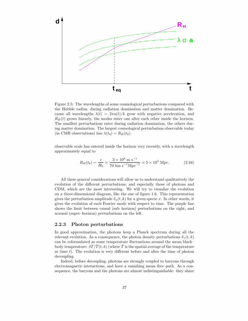
λ α a

t

d

t

RH

eq

Figure 2.5: The wavelengths of some cosmological perturbations compared withthe Hubble radius, during radiation domination and matter domination. Be-cause all wavelengths λ(t) = 2πa(t)/k grow with negative acceleration, andRH(t) grows linearly, the modes enter one after each other inside the horizon.The smallest perturbations enter during radiation domination, the others dur-ing matter domination. The largest cosmological perturbation observable today(in CMB observations) has λ(t0) = RH(t0).

observable scale has entered inside the horizon very recently, with a wavelengthapproximately equal to

RH(t0) =c

H0' 3 × 108 m s−1

70 km s−1Mpc−1' 5 × 103 Mpc. (2.34)

All these general considerations will allow us to understand qualitatively theevolution of the different perturbations, and especially those of photons andCDM, which are the most interesting. We will try to visualize the evolutionon a three-dimensional diagram, like the one of figure 1.6. This representationgives the perturbation amplitude δx(t, k) for a given specie x. In other words, itgives the evolution of each Fourier mode with respect to time. The purple lineshows the limit between causal (sub–horizon) perturbations on the right, andacausal (super–horizon) perturbations on the left.

2.2.3 Photon perturbations

In good approximation, the photons keep a Planck spectrum during all therelevant evolution. As a consequence, the photon density perturbations δγ(t, k)can be reformulated as some temperature fluctuations around the mean black–body temperature: δT/T (t, k) (where T is the spatial average of the temperatureat time t). The evolution is very different before and after the time of photondecoupling.

Indeed, before decoupling, photons are strongly coupled to baryons throughelectromagnetic interactions, and have a vanishing mean–free–path. As a con-sequence, the baryons and the photons are almost indistinguishable: they share

37

t eq

2 π aRH

k

CA

USA

L

AC

AU

SAL

large wavelength

small w

avelength

radiation domination

matter domination

t

perturbation

Figure 2.6: For any specie, this type of diagram can be used for understandingqualitatively the evolution of the Fourier spectrum as a function of time. EachFourier mode of fixed comoving wavenumber k enters into the causal horizonwhen it crosses the purple line (which corresponds to λ(t) = RH(t), i.e., tok = 2πa(t)/RH(t)).

the same density perturbations, and can be viewed as single fluid. In addi-tion, since baryons have a mass, they feel gravitational forces: so, the entirebaryon–photon fluid is coupled with the gravitational potential.

So, in each well of gravitational potential, the baryon–photon fluid tends tobe compressed by gravity, but the relativistic photon pressure p = 1

3ρ tends toresist to this compression. The dynamics of the fluid is governed by two antago-nist forces, as for any oscillator. So, for each Fourier mode, any departure fromequilibrium – such as a non–zero initial perturbation – will lead to oscillations.These oscillations propagate through the fluid exactly like sound waves in theair: due to this analogy, the perturbations in the baryon–photon fluid beforedecoupling are called acoustic oscillations.

Of course, the oscillations can occur only for causal wavelengths: because ofcausality, wavelengths bigger than the Hubble radius do not feel any force. So, agiven mode with a given non–zero initial amplitude starts oscillating only whenit enters into the horizon (see figure 2.7). The initial amplitude for each modeat initial time is given by the primordial spectrum of perturbations. Of course, ifthe Universe was perfectly homogeneous from the very beginning (with no initialperturbations), there would be no acoustic oscillations – and no formation ofstructure either, so we must assume some primordial perturbations. At this

38

2 π aRH

k

t

decoupling

perturbation ( T/T )γ δ

Figure 2.7: Evolution of the Fourier spectrum of photon temperature fluctu-ations, as a function of time. We start from a flat primordial spectrum, aspredicted by inflation and as confirmed by observations. When a given Fouriermode enters inside the horizon (i.e., crosses the dashed purple line), it startsto oscillate. At decoupling, the temperature distribution is frozen (later, alltemperatures are redshifted by a factor 1/a(t), so the relative fluctuation δT/Tremains constant). So, the Fourier spectrum measured today is the same as atthe time of decoupling. It exhibits a flat plateau for wavelengths bigger than theHubble radius at decoupling, and then a series of peaks called acoustic peaks.

stage, the primordial spectrum has to be assumed arbitrarily. Only in the lastsection, we will see a precise mechanism called “inflation” leading to a givenprimordial spectrum. On figure 2.7, we start from a flat spectrum, independentof k – in good approximation, this corresponds to what is observed today, andalso to what is predicted by the theory of inflation.

When the photons decouple from the matter, their mean–free–path growsrapidly from zero ton infinity, and they travel in straight line with essentially nointeraction. During this free-streaming, all their characteristics – momentum,energy, wavelength, spectrum, temperature – do not evolve, excepted under theeffect of homogeneous expansion. So, δT and T are both shifted proportionallyto 1/a(t), but the distribution of δT/T (t, k) observed today is exactly the sameas at the time of decoupling. Observing the temperature anisotropies in the skyamounts exactly in taking a picture of the Universe at the time of decoupling.

So, in order to know the present Fourier spectrum of temperature fluctua-

39

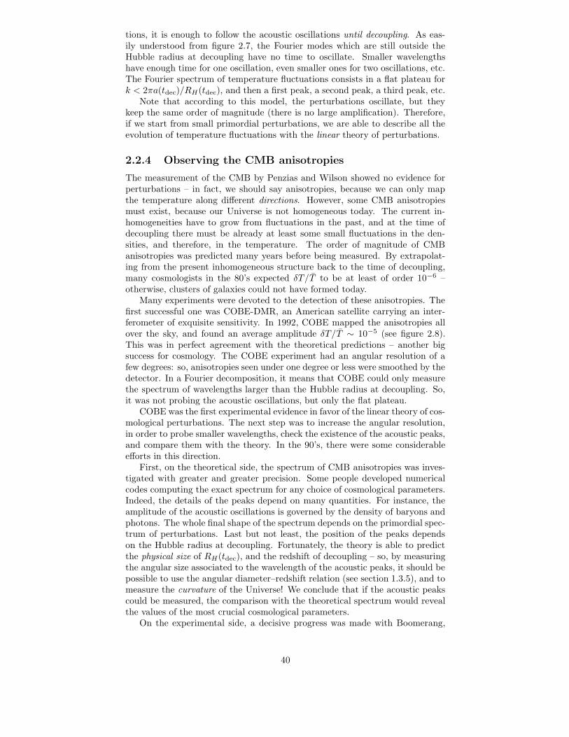
tions, it is enough to follow the acoustic oscillations until decoupling. As eas-ily understood from figure 2.7, the Fourier modes which are still outside theHubble radius at decoupling have no time to oscillate. Smaller wavelengthshave enough time for one oscillation, even smaller ones for two oscillations, etc.The Fourier spectrum of temperature fluctuations consists in a flat plateau fork < 2πa(tdec)/RH(tdec), and then a first peak, a second peak, a third peak, etc.

Note that according to this model, the perturbations oscillate, but theykeep the same order of magnitude (there is no large amplification). Therefore,if we start from small primordial perturbations, we are able to describe all theevolution of temperature fluctuations with the linear theory of perturbations.

2.2.4 Observing the CMB anisotropies

The measurement of the CMB by Penzias and Wilson showed no evidence forperturbations – in fact, we should say anisotropies, because we can only mapthe temperature along different directions. However, some CMB anisotropiesmust exist, because our Universe is not homogeneous today. The current in-homogeneities have to grow from fluctuations in the past, and at the time ofdecoupling there must be already at least some small fluctuations in the den-sities, and therefore, in the temperature. The order of magnitude of CMBanisotropies was predicted many years before being measured. By extrapolat-ing from the present inhomogeneous structure back to the time of decoupling,many cosmologists in the 80’s expected δT/T to be at least of order 10−6 –otherwise, clusters of galaxies could not have formed today.

Many experiments were devoted to the detection of these anisotropies. Thefirst successful one was COBE-DMR, an American satellite carrying an inter-ferometer of exquisite sensitivity. In 1992, COBE mapped the anisotropies allover the sky, and found an average amplitude δT/T ∼ 10−5 (see figure 2.8).This was in perfect agreement with the theoretical predictions – another bigsuccess for cosmology. The COBE experiment had an angular resolution of afew degrees: so, anisotropies seen under one degree or less were smoothed by thedetector. In a Fourier decomposition, it means that COBE could only measurethe spectrum of wavelengths larger than the Hubble radius at decoupling. So,it was not probing the acoustic oscillations, but only the flat plateau.

COBE was the first experimental evidence in favor of the linear theory of cos-mological perturbations. The next step was to increase the angular resolution,in order to probe smaller wavelengths, check the existence of the acoustic peaks,and compare them with the theory. In the 90’s, there were some considerableefforts in this direction.

First, on the theoretical side, the spectrum of CMB anisotropies was inves-tigated with greater and greater precision. Some people developed numericalcodes computing the exact spectrum for any choice of cosmological parameters.Indeed, the details of the peaks depend on many quantities. For instance, theamplitude of the acoustic oscillations is governed by the density of baryons andphotons. The whole final shape of the spectrum depends on the primordial spec-trum of perturbations. Last but not least, the position of the peaks dependson the Hubble radius at decoupling. Fortunately, the theory is able to predictthe physical size of RH(tdec), and the redshift of decoupling – so, by measuringthe angular size associated to the wavelength of the acoustic peaks, it should bepossible to use the angular diameter–redshift relation (see section 1.3.5), and tomeasure the curvature of the Universe! We conclude that if the acoustic peakscould be measured, the comparison with the theoretical spectrum would revealthe values of the most crucial cosmological parameters.

On the experimental side, a decisive progress was made with Boomerang,

40

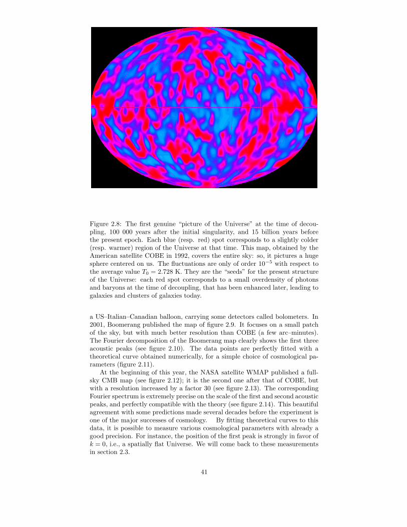
Figure 2.8: The first genuine “picture of the Universe” at the time of decou-pling, 100 000 years after the initial singularity, and 15 billion years beforethe present epoch. Each blue (resp. red) spot corresponds to a slightly colder(resp. warmer) region of the Universe at that time. This map, obtained by theAmerican satellite COBE in 1992, covers the entire sky: so, it pictures a hugesphere centered on us. The fluctuations are only of order 10−5 with respect tothe average value T0 = 2.728 K. They are the “seeds” for the present structureof the Universe: each red spot corresponds to a small overdensity of photonsand baryons at the time of decoupling, that has been enhanced later, leading togalaxies and clusters of galaxies today.

a US–Italian–Canadian balloon, carrying some detectors called bolometers. In2001, Boomerang published the map of figure 2.9. It focuses on a small patchof the sky, but with much better resolution than COBE (a few arc–minutes).The Fourier decomposition of the Boomerang map clearly shows the first threeacoustic peaks (see figure 2.10). The data points are perfectly fitted with atheoretical curve obtained numerically, for a simple choice of cosmological pa-rameters (figure 2.11).

At the beginning of this year, the NASA satellite WMAP published a full-sky CMB map (see figure 2.12); it is the second one after that of COBE, butwith a resolution increased by a factor 30 (see figure 2.13). The correspondingFourier spectrum is extremely precise on the scale of the first and second acousticpeaks, and perfectly compatible with the theory (see figure 2.14). This beautifulagreement with some predictions made several decades before the experiment isone of the major successes of cosmology. By fitting theoretical curves to thisdata, it is possible to measure various cosmological parameters with already agood precision. For instance, the position of the first peak is strongly in favor ofk = 0, i.e., a spatially flat Universe. We will come back to these measurementsin section 2.3.

41

Figure 2.9: The map of CMB anisotropies obtained by the balloon experimentBoomerang in 2001. Unlike COBE, Boomerang only analyzed a small patch ofthe sky, but with a much better angular resolution of a few arc–minutes. Theblack (resp. yellow) spots correspond to colder (resp. warmer) regions.

There are still many CMB experiments going on. The satellite WMAPgoes on acquiring data in order to reach even better resolution. In 2007, theEuropean satellite “Planck” will be launched. Planck is expected to performthe best possible measurement of the CMB temperature anisotropies, with suchgreat precision that most cosmological parameters should be measured withonly one per cent uncertainty.

2.2.5 Matter perturbations

We now focus on the evolution of the matter perturbations. Because we believethat the Universe contains much more CDM than baryons, in first approxima-tion, we can forget the baryons, and do as if all the matter was in the form ofCDM, with absolutely no electromagnetic interactions. This is crucial, becausein absence of any coupling with the photons, the CDM fluid has a vanishingpressure: so, it tends to concentrate in each well of gravitational potential –instead of oscillating like the baryons before decoupling. This is called gravita-tional collapse.

Of course, as all causal mechanisms, gravitational collapse can only affectmodes inside the Hubble radius. However, there is one more restriction. Duringmatter domination, when a potential well appears, CDM concentrates in it, anddeepens the gravitational potential even more. So, both CDM and gravitationalpotential perturbations are quickly amplified. On the other hand, during radi-ation domination, the gravitational potential follows the perturbations of thedominant energy density: that of radiation. So, there is no significant coupling

42

Figure 2.10: The Fourier decomposition of the Boomerang map reveals thestructure of the first three acoustic oscillations. These data points account forthe spectrum of (δT )2 in (µK)2 – we know from COBE that δT is roughly oforder 10−5T0 ' 30 µK. The spectrum is not shown as a function of wavenumberk, but of multipole number l. This is because the anisotropies are not observedin 3-dimensional space, but on a two-dimensional sphere: the sphere of redshiftz ∼ 1000 centered on us. For purely geometric reasons, a spherical map isnot expandable in Fourier modes, but in Legendre multipoles. However, theinterpretation is the same. The first, second and third peak correspond to themodes that could oscillate one, two or three times between their entry into theHubble radius and the time of decoupling.

between the CDM inhomogeneities and the gravitational potential. As a conse-quence, the amplification of CDM perturbations is efficient only after equalityand inside RH . If we look at the diagram of figure 2.6, this corresponds tothe region on the right of the purple curve, and below the yellow line. So,even today, the Fourier spectrum of CDM perturbations has a characteristicscale corresponding to the Hubble radius at equality. The same type of numer-ical code which compute the spectrum of CMB anisotropies can also computethe linear matter spectrum with great precision, for any choice of cosmologicalparameters.

But linear perturbation theory is valid only as long as the perturbationsare small, δCDM(t, k) 1. After, it is no longer interesting to use a Fourierdecomposition, because the evolution of each mode is not independent of theothers: so, everything becomes much more complicated, and we can make somepredictions only from numerical simulations of the gravitational collapse in realspace. These are called an N-body simulations.

It is crucial to know at what time a given mode enters into the non-linearregime, δCDM(t, k) ∼ 1. If there was absolutely no growth of CDM perturba-

43

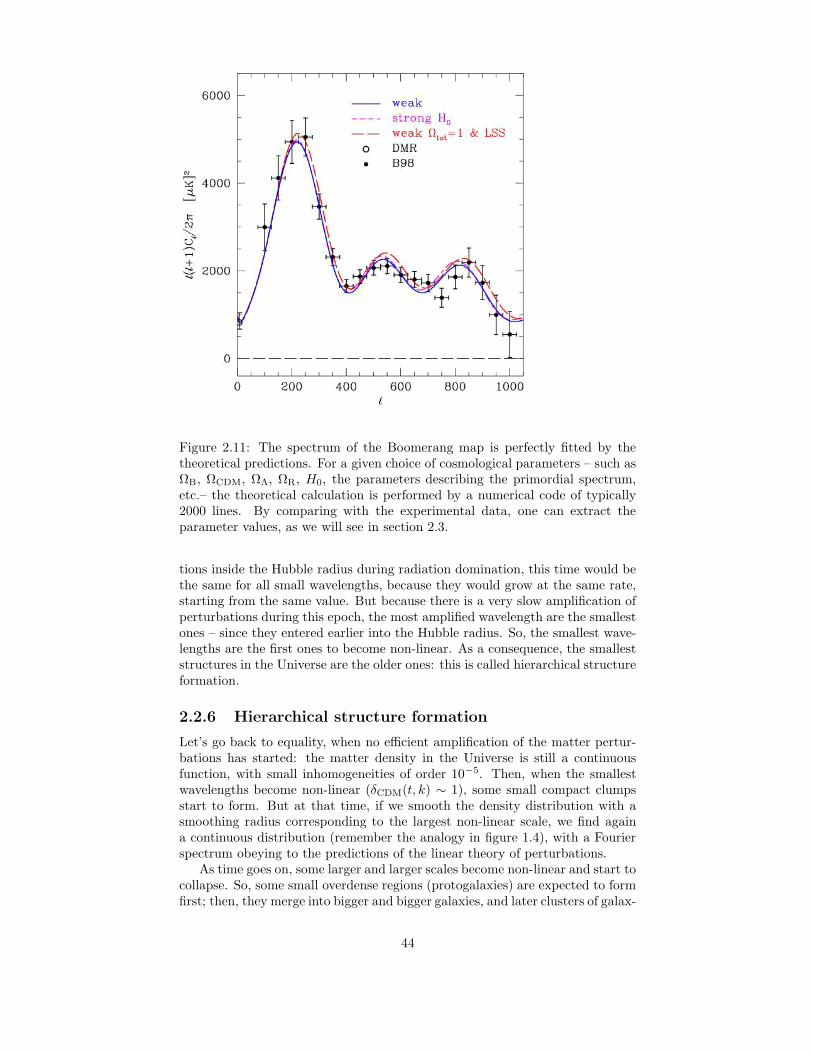
Figure 2.11: The spectrum of the Boomerang map is perfectly fitted by thetheoretical predictions. For a given choice of cosmological parameters – such asΩB, ΩCDM, ΩΛ, ΩR, H0, the parameters describing the primordial spectrum,etc.– the theoretical calculation is performed by a numerical code of typically2000 lines. By comparing with the experimental data, one can extract theparameter values, as we will see in section 2.3.

tions inside the Hubble radius during radiation domination, this time would bethe same for all small wavelengths, because they would grow at the same rate,starting from the same value. But because there is a very slow amplification ofperturbations during this epoch, the most amplified wavelength are the smallestones – since they entered earlier into the Hubble radius. So, the smallest wave-lengths are the first ones to become non-linear. As a consequence, the smalleststructures in the Universe are the older ones: this is called hierarchical structureformation.

2.2.6 Hierarchical structure formation

Let’s go back to equality, when no efficient amplification of the matter pertur-bations has started: the matter density in the Universe is still a continuousfunction, with small inhomogeneities of order 10−5. Then, when the smallestwavelengths become non-linear (δCDM(t, k) ∼ 1), some small compact clumpsstart to form. But at that time, if we smooth the density distribution with asmoothing radius corresponding to the largest non-linear scale, we find againa continuous distribution (remember the analogy in figure 1.4), with a Fourierspectrum obeying to the predictions of the linear theory of perturbations.

As time goes on, some larger and larger scales become non-linear and start tocollapse. So, some small overdense regions (protogalaxies) are expected to formfirst; then, they merge into bigger and bigger galaxies, and later clusters of galax-

44

Figure 2.12: The full-sky map of CMB anisotropies obtained by the satelliteWMAP in 2003. The blue (resp. red) spots correspond to colder regions. Thismap has been cleaned from any foreground contamination, including that of theMilky Way: it only shows the CMB contribution.

ies will also appear. Finally, in the present Universe, the scale of non-linearityis expected to be around 20 or 40 Mpc. This is one order of magnitude biggerthan clusters of galaxies: so, even the clusters are not smoothly distributed. Infact, they tend to organize themselves along huge filaments, separated by voidsof size 20 to 40 Mpc. The structure of the Universe on these huge scales looksvery much like a spounge... But by smoothing the present distribution of matterover scales larger than 40 Mpc, one finds again a continuous distribution, withsmall inhomogeneities described by the linear Fourier spectrum of cosmologicalperturbation theory.

2.2.7 Observing the matter spectrum

So, if we have a large three–dimensional map of the galaxy distribution in theUniverse, we can smooth it on very large scales, compare with the linear spec-trum predicted by the theory, and measure the cosmological parameters onwhich this spectrum depends. Of course, what we observe in the sky is only lu-minous baryonic matter, not CDM. But astrophysicists have very good reasonsto believe that on large scales, the distribution of luminous matter “traces” thedistribution of mass. This means that the inhomogeneities in luminous mat-ter would be proportional to the total density inhomogeneities – i.e., in goodapproximation, to the CDM inhomogeneities. The unknown coefficient of pro-portionality is called the bias b:

δluminous(t, k) ' b δCDM(t, k). (2.35)

Over the past decades, astronomers could build some very large three-dimensional maps of the galaxy distribution – even larger than the scale ofnon-linearity. On figure 2.15, we can see two thin “slices” of the surroundingUniverse. Inside these slices, each point corresponds to a galaxy seen by the“2dF Galaxy Redshift Survey”. The radial coordinate is the redshift, or thedistance between the object and us. Even at redshift z < 0.1, we can see some

45

Figure 2.13: Comparison between the COBE and WMAP anisotropy maps. Inboth figure, the red stripe in the middle is the foreground contamination fromthe Milky Way. The orientation of the two maps is the same in order to allowfor direct visual comparison. The resolution of WMAP is 30 times better, butit is clear that on large angular scale, the two maps reveal the same structure.

darker regions, corresponding to the voids - the largest non-linear structures inthe Universe. At z > 0.1, the average density seems to decrease smoothly, butthis is simply because the survey is limited in sensitivity – at small distanceit sees all the galaxies, while at large distance it sees only the brightest ones.By taking this selection effect into account, and by smoothing over distances oforder of 50 Mpc, one recovers a very homogeneous distribution of matter.

On figure 2.16, we see the Fourier spectrum reconstructed from such a red-shift survey. Each experimental point is obtained by smoothing over smallerwavelengths. The data points with k < 0.2h Mpc−1 can be directly comparedwith the linear spectrum predicted by the linear theory of cosmological pertur-bations. The red line shows one of the best-fit theoretical curves. From such acomparison, one can extract some information on the value of the cosmologicalparameters. This is similar to the parameter extraction from CMB anisotropies,

46

Figure 2.14: The spectrum of WMAP map is perfectly fitted by the theoreticalpredictions, for a given choice of cosmological parameters – namely, for themodel showed here, ΩB, ΩCDM, ΩΛ, the so-called “optical depth to reionization”(a quantity not defined in this course), and the two parameters describing apower-law primordial spectrum.

but it provides some independent constraints.On the extreme left of figure 2.16, we see that the theoretical curve reaches

a maximum (around k ∼ 0.01h Mpc−1, i.e., λ ∼ 400 Mpc). This corresponds tothe scale which entered into the Hubble radius at the time of equality betweenradiation and matter. Future redshift surveys are expected to give better dataaround this scale. Observing the turnover of the matter spectrum with goodprecision will improve the measurement of the cosmological parameters.

2.3 Measuring the cosmological parameters

There has been some continuous progress in measuring the cosmological param-eters over the past three decades; however, the most spectacular improvementshave been made in the last five years. Many techniques can be employed forconstraining the cosmological scenarios – probably around twenty. Instead ofgiving an exhaustive review, we will focus only on five important methods.

2.3.1 Abundance of primordial elements

In sections 2.1.3 and 2.1.5, we have seen that the theory of Nucleosynthesis canpredict the abundance of light elements formed in the early Universe, when theenergy density was of order ρ ∼ (1MeV)4. This theory has reached today agreat level of precision: it is believed that each relevant nuclear reaction aretaken carefully into account. In the standard model of Nucleosynthesis, thereare only two free parameters: the baryon density ρB, or equivalently, ΩBh2;

47

Figure 2.15: The distribution of galaxies in two thin slices of the neighboringUniverse, obtained by the 2dF Galaxy Redshift Survey. The radial coordinateis the redshift, or the distance between the object and us.

and the number of neutrino families Nν . For each value of the baryon densityand of Nν , the theory predicts a given abundance of hydrogen, helium, lithium,etc. So, by observing the abundance of these elements in the Universe – forinstance, using spectroscopy – it is possible to constrain the baryon density.Current observations lead to the prediction

ΩBh2 = 0.020± 0.002. (2.36)

Moreover, they are perfectly compatible with Nν = 3, which is known fromaccelerator physics to be the number of neutrino families.

2.3.2 CMB anisotropies

The precise dynamics of the acoustic oscillations before decoupling depends onalmost all the cosmological parameters: so, the spectrum of CMB anisotropiescan give a wide variety of constraints. This type of experiment is considered as

48

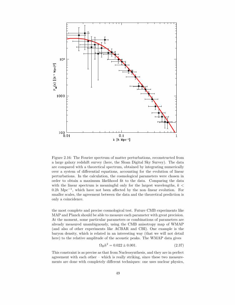
Figure 2.16: The Fourier spectrum of matter perturbations, reconstructed froma large galaxy redshift survey (here, the Sloan Digital Sky Survey). The dataare compared with a theoretical spectrum, obtained by integrating numericallyover a system of differential equations, accounting for the evolution of linearperturbations. In the calculation, the cosmological parameters were chosen inorder to obtain a maximum likelihood fit to the data. Comparing the datawith the linear spectrum is meaningful only for the largest wavelengths, k <0.2h Mpc−1, which have not been affected by the non–linear evolution. Forsmaller scales, the agreement between the data and the theoretical prediction isonly a coincidence.

the most complete and precise cosmological test. Future CMB experiments likeMAP and Planck should be able to measure each parameter with great precision.At the moment, some particular parameters or combinations of parameters arealready measured unambiguously, using the CMB anisotropy map of WMAP(and also of other experiments like ACBAR and CBI). One example is thebaryon density, which is related in an interesting way (that we will not detailhere) to the relative amplitude of the acoustic peaks. The WMAP data gives

ΩBh2 = 0.022± 0.001. (2.37)

This constraint is as precise as that from Nucleosynthesis, and they are in perfectagreement with each other – which is really striking, since these two measure-ments are done with completely different techniques: one uses nuclear physics,

49

applied to the Universe when it had a density of order (1 Mev)4, while the otheruses fluid mechanics, applied to a much more recent era with density (0.1 eV)4.The perfect overlap between the two constraints indicates that our knowledgeof the Universe is impressively good, at least during the epoch between t ∼ 1 sand t ∼ 100 000 yr.

We have seen that the position of the acoustic peak is given by the Hubbleradius at decoupling, which value is predicted by the theory. So, using theangular diameter–redshift relation (see section 1.3.5), it is possible to extractsome information both on the spatial curvature and on the evolution of thescale factor a(t). A detailed study shows that the leading effect is that ofspatial curvature. So, the position of the acoustic peak gives a measurement ofΩk = 1 − Ω0. The result is

Ω0 = 1.03± 0.05. (2.38)

So, according to current CMB experiments, the Universe seems to be spatiallyflat. This result is extremely useful, but it doesn’t say how the present energydensity is distributed between matter and a possible cosmological constant2.

Current CMB experiments also give other interesting constraints (for in-stance, on the primordial spectrum of perturbations) that we will not explainhere.

2.3.3 Age of the Universe

Observations can set a reliable lower bound on the age of the Universe: if anobject is seen at a given redshift, corresponding to a given age, the Universe hasto be older than this object. During the 1990’s, it has been established that themost distant observable quasars are at least 11 Gyr old. On the other hand, aspatially flat matter–dominated Universe would be only 9 Gyr old (see section2.1.6). So, distant quasars seem to indicate that the Universe is either open orΛ–dominated today.

2.3.4 Luminosity of Supernovae

The evidence for a non–flat Universe and/or a non–zero cosmological constanthas increased considerably in 1998, when two independent groups studied theapparent luminosity of distant type Ia supernovae (SNIa). For this type ofsupernovae, astronomers believe that there is a simple relation between theabsolute magnitude and the luminosity decay rate. In other words, by studyingthe rise and fall of the luminosity curve during a few weeks, one can deduce theabsolute magnitude of a given SNIa. Therefore, it can be used in the same wayas cepheid, as a probe of the apparent luminosity–redshift relation. In addition,Supernovae are much brighter that cepheids, and can be observed at muchlarger distances (until redshifts of order one). While observable cepheids onlyprobe short distances, where the apparent luminosity–redshift relation only givesthe Hubble law (the proportionality between distance and redshift), the mostdistant observable SNIa’s are in the region where general relativity correctionsare important: so, they can provide a measurement of the spatial curvature andof the scale factor evolution.

On figure 2.17, the various curves represent the apparent magnitude–redshiftrelation, computed for various choices of ΩM and ΩΛ. For a given value of H0,all the curves are asymptotically equal at short distance. Significant differencesshow up only at redshifts z > 0.2. Each red data point corresponds to a single

2As far as radiation is concerned, we know that today, it is negligible with respect tomatter, so that Ω0 ' ΩM + ΩΛ = ΩB + ΩCDM + ΩΛ.

50

Calan/Tololo (Hamuy et al, A.J. 1996)

Supernova Cosmology Project

effe

ctiv

e m

B

(0.5,0.5) (0, 0)( 1, 0 ) (1, 0)(1.5,–0.5) (2, 0)

(ΩΜ,ΩΛ) = ( 0, 1 )

Flat

Λ =

0

redshift z

14

16

18

20

22

24

26

0.02 0.05 0.1 0.2 0.5 1.00.02 0.05 0.1 0.2 0.5 1.0

Perlmutter, et al. (1998)F

AIN

TE

R

(Far

ther

) (F

urt

her

bac

k in

tim

e)

MORE REDSHIFT (More total expansion of universe since the supernova explosion)

In flat universe: ΩM = 0.28 [± 0.085 statistical] [± 0.05 systematic]

Prob. of fit to Λ = 0 universe: 1%

Figure 2.17: The results published by the “Supernovae Cosmology Project” in1998. The various curves represent the apparent magnitude–redshift relation,computed for various choices of ΩM and ΩΛ. The solid black curves account forthree examples of a closed/flat/open Universe with no cosmological constant.The dashed blue curves correspond to three spatially flat universes with differentvalues of ΩΛ. For a given value of H0, all the curves are asymptotically equalat short distance, probing only the Hubble law. The yellow points are short–distance SNIa’s: we can check that they are approximately aligned. The redpoints, at redshifts between 0.2 and 0.9, show that distant supernovae are tooluminous to be compatible with a flat matter-dominated Universe (ΩM, ΩΛ)=(1,0).

supernovae, from the 1998 results of the “Supernovae Cosmology Project”. Evenif it is not very clear visually from the figure, a detailed statistical analysis revealsthat a flat matter–dominated Universe (with ΩM = 1, ΩΛ = 0) is excluded. Thisresult has been confirmed by more recent data at larger redshift. According to

51

Figure 2.18: Combined constraints on (ΩM, ΩΛ) from CMB and Supernovaeexperiments. The simple case of a spatially flat Universe with no cosmologicalconstant corresponds to the lower right corner of the plot. In blue, the CMBallowed region favors a spatially flat Universe with ΩM +ΩΛ ' 1. In orange, theSupernovae constraint is orthogonal to the CMB one. By combining the tworesults, one obtains the favored region limited by the black ellipses, centerednear (ΩM, ΩΛ) = (0.3, 0.7).

statistical analysis, the allowed region in the (ΩM, ΩΛ) parameter space is

−1 < ΩM − ΩΛ < 0. (2.39)

When this observation is combined with the CMB results (figure 2.18), itappears that our Universe is spatially flat and has a non–zero cosmologicalconstant – a case corresponding to accelerated expansion today! The favoredvalues are (ΩM, ΩΛ) = (0.3,0.7).

2.3.5 Large Scale Structure

We have seen that the Fourier spectrum of matter perturbations on very largescales (figure 2.16) depends on the cosmological parameters. Current galaxyredshift surveys provide some constraints which are essentially independent fromthose of the previous sections. It is remarkable that they converge toward thesame values as the previous techniques.

52

In conclusion, current experiments agree on the following matter budget inthe present Universe:

Ω0 = ΩB + ΩCDM + ΩΛ ' 1ΩΛ ' 0.73ΩB ' 0.04

So, the Universe seems to be accelerating today, and 96% of its energy densityis non–baryonic and of essentially unknown nature! The measured value ofthe cosmological constant shows that the Universe started to be Λ–dominatedonly recently: at redshifts z ≥ 2, the Universe was still matter–dominated. Weseem to be leaving precisely during the period of transition between matter–domination and Λ–domination!

2.4 The Inflationary Universe

2.4.1 Problems with the Standard Cosmological Model

According to the modern version of the standard cosmological model, calledthe ΛCDM model, the Universe is spatially flat, with three stages: radiation–domination before z ∼ 104, matter–domination, and now, transition to Λ–domination. This scenario is impressively successful in explaining a wide va-riety of observations, as we could see in section 2.3. However, it also raises afew problems.

The flatness problem.The present contribution of the spatial curvature to the expansion is given byΩk = ρ0(t0)/ρc(t0) − 1. But this contribution has evolved with time. From theFriedmann law, it is straightforward to see that

|Ωk(t)| = |ρ0(t)/ρc(t) − 1| =c2|k|a2H2

=c2|k|a2

. (2.40)

During the domination of radiation (resp. matter), the factor a−2 grows liket (resp. t2/3). Therefore, a spatially flat Universe is unstable: if initially, kis exactly zero, Ωk will remain zero; but if it is only close to zero, Ωk willincrease with time! In order to have no significant curvature–domination today(|Ωk(t0)| ≤ 0.1), we find that near the Planck time, the curvature was incrediblysmall, roughly |Ωk(t)| ≤ 10−60... The standard cosmological model provides noexplanation for obtaining such a small number in the early Universe: the factthat the Universe is spatially flat – even approximately – appears like the mostunnatural possibility! This is called the “flatness problem”.

The horizon problem.We have seen that during radiation and matter domination, the causal horizon isequal to the Hubble radius (times a factor 2 or 4). From the observation of CMBanisotropies, we know that the Hubble radius at the time of decoupling is seentoday under an angle of one degree in the sky. So, on CMB maps, two pointsseen under an angle bigger than one degree seem to be be causally disconnected.In other words, the CMB maps seem to be composed of approximately 103

independent regions, which could not exchange any information in the past.But then, how can they be at the same temperature – up to 10−5 ? Given thesetheoretical arguments, we would rather expect each of these regions to have itsown temperature. Then, today we would observe inhomogeneities of order one.Measuring approximately the same temperature T0 = 2.73 K all over the skyappears like a big mystery called the “horizon problem”.

53

The origin of fluctuations.The horizon problem can be reformulated in a slightly different way. We haveseen on figure 2.5 that during radiation and matter domination, the Hubbleradius (and the causal horizon) grow faster than the physical wavelength ofeach perturbation. So, all the wavelengths observable today on cosmologicalscales were larger than the horizon in the early Universe. So far, we did notpropose any mechanism for the generation of primordial perturbations. But wehave the following problem: if primordial perturbations are acausal, how canthey be generated without violating causality (i.e., the fact that no informationcan travel faster than the speed of light)?

The Cosmic Coincidence problem.We have seen that the cosmological constant starts to dominate the energydensity of the Universe only in the very near past. Why are we leaving just at

the time of the transition? If ΩΛ is of order one, then ρ1/4Λ is of order 10−3 eV.

Any vacuum energy density resulting from a spontaneous symmetry breakingin the standard model of particle physics should be at least of the order of theelectroweak scale, near 1 TeV. Eventually, some unknown symmetry could forcethe vacuum energy to vanish exactly. But why should it be as small as 10−3 eV?

So, particle physics seems to be easily compatible with a Universe that wouldbe either completely matter-dominated or completely Λ–dominated today. Butthe subtle balance observed between ordinary matter and the cosmological con-stant appears as extremely unnatural and mysterious.

2.4.2 An initial stage of inflation

So, the standard cosmological model raises a series of problem – the previouslist is not exhaustive. We will see that many of them can be solved in an elegantway.

Let us assume that in the early Universe, before radiation domination, therehas been a stage of accelerating expansion: a > 0. So far, we don’t say whichmechanism could be responsible for this period, called inflation. If a is positive,a increases, and according to equation (2.40), |Ωk| decreases. The contributionof the spatial curvature to the expansion is driven to zero. This provides apossible solution to the flatness problem: during the initial inflationary stage,|Ωk| becomes extremely small. Then, it grows again, but today it might still bevery far from order one.

The simple relation that we found between the causal horizon and the Hub-ble radius is not true anymore during inflation. As a particular example ofaccelerated expansion, let us assume that a(t) grows exponentially:

a(t) = eHit. (2.41)

In that case, the Hubble radius is constant:

RH = c

(

a

a

)

−1

=c

Hi, (2.42)

while the causal horizon grows exponentially:

dH (t1, t2) = 2a(t2)

∫ t2

t1

c dt

a(t)−→ c

HieH(t2−t1) when t2 t1. (2.43)

So, at the end of an inflation, the causal horizon is much bigger than the Hubbleradius. After, during radiation and matter domination, they grow at the samerate, and the causal horizon remains larger. So, an initial stage of inflation can

54

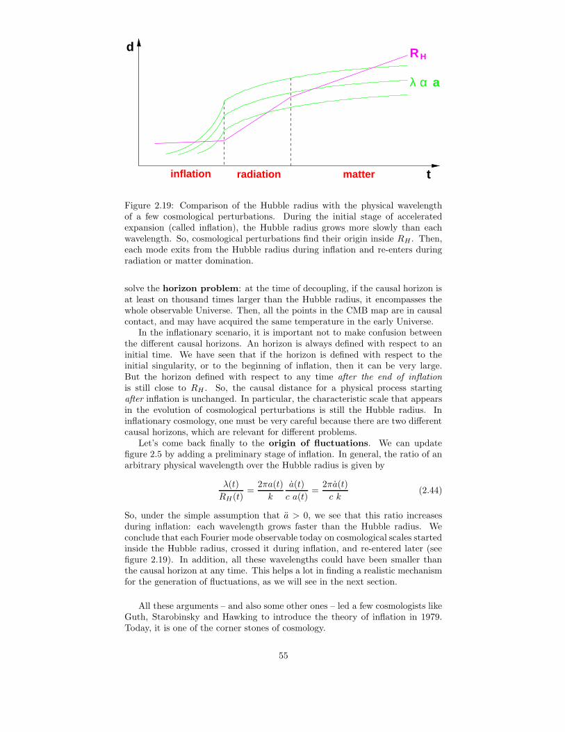
inflation radiation matter

λ α a

d

t

RH

Figure 2.19: Comparison of the Hubble radius with the physical wavelengthof a few cosmological perturbations. During the initial stage of acceleratedexpansion (called inflation), the Hubble radius grows more slowly than eachwavelength. So, cosmological perturbations find their origin inside RH . Then,each mode exits from the Hubble radius during inflation and re-enters duringradiation or matter domination.

solve the horizon problem: at the time of decoupling, if the causal horizon isat least on thousand times larger than the Hubble radius, it encompasses thewhole observable Universe. Then, all the points in the CMB map are in causalcontact, and may have acquired the same temperature in the early Universe.

In the inflationary scenario, it is important not to make confusion betweenthe different causal horizons. An horizon is always defined with respect to aninitial time. We have seen that if the horizon is defined with respect to theinitial singularity, or to the beginning of inflation, then it can be very large.But the horizon defined with respect to any time after the end of inflation

is still close to RH . So, the causal distance for a physical process startingafter inflation is unchanged. In particular, the characteristic scale that appearsin the evolution of cosmological perturbations is still the Hubble radius. Ininflationary cosmology, one must be very careful because there are two differentcausal horizons, which are relevant for different problems.

Let’s come back finally to the origin of fluctuations. We can updatefigure 2.5 by adding a preliminary stage of inflation. In general, the ratio of anarbitrary physical wavelength over the Hubble radius is given by

λ(t)

RH(t)=

2πa(t)

k

a(t)

c a(t)=

2πa(t)

c k(2.44)

So, under the simple assumption that a > 0, we see that this ratio increasesduring inflation: each wavelength grows faster than the Hubble radius. Weconclude that each Fourier mode observable today on cosmological scales startedinside the Hubble radius, crossed it during inflation, and re-entered later (seefigure 2.19). In addition, all these wavelengths could have been smaller thanthe causal horizon at any time. This helps a lot in finding a realistic mechanismfor the generation of fluctuations, as we will see in the next section.

All these arguments – and also some other ones – led a few cosmologists likeGuth, Starobinsky and Hawking to introduce the theory of inflation in 1979.Today, it is one of the corner stones of cosmology.

55

2.4.3 Scalar field inflation

So, the first three problems of section 2.4.1 can be solved under the assumptionof a long enough stage of accelerated expansion in the early Universe. How canthis be implemented in practice?

First, by combining the Friedman equation (1.30) in a flat Universe with theconservation equation (1.32), it is easy to find that

a > 0 ⇒ ρ + 3p < 0. (2.45)

What type of matter corresponds to such an unusual relation between densityand pressure? A positive cosmological constant can do the job:

pΛ = −ρΛ ⇒ ρΛ + 3pΛ = −2ρΛ < 0. (2.46)

But since a cosmological constant is... constant, it cannot be responsible foran initial stage of inflation: otherwise this stage would go on forever, and therewould be no transition to radiation domination.

Let us consider instead the case of a scalar field (i.e., a field of spin zero,represented by a simple function of time and space, and invariant under Lorentztransformations). In general, for a homogeneous scalar field ϕ(t), the densityand pressure read

ρ =1

2ϕ2 + V (ϕ), (2.47)

p =1

2ϕ2 − V (ϕ), (2.48)

where V is the scalar potential. So, the pressure is equal to the kinetic energyminus the potential energy. We see that in the limit – called slow–roll – wherethe kinetic energy is subdominant, the pressure is close to −ρ, and the fieldbehaves almost like a cosmological constant. However, the field is still slowlyrolling toward the minimum of its potential – which should have a small slope,otherwise the kinetic energy would be leading.

So, a particular way to obtain a stage of accelerated expansion in the earlyUniverse is to introduce a scalar field, with a flat enough potential. Scalar fieldinflation has been proposed in 1979 by Guth. During the 80’s, most importantaspects of inflation were studied in details, by Guth, Starobinsky, Hawking,Linde and other people. Finally, during the 90’s, many ideas and models wereproposed in order to make contact between inflation and particle physics. Thepurpose of scalar field inflation is not only to provide a stage of acceleratedexpansion in the early Universe, but also, a mechanism for the generation ofmatter and radiation particles, and another mechanism for the generation ofprimordial cosmological perturbations. Let us summarize how it works in avery sketchy way.

Slow-roll.First, let us assume that just after the initial singularity, the energy density

is dominated by a scalar field, with a potential flat enough for slow–roll. In anysmall region where the field is approximately homogeneous and slowly–rolling,accelerated expansion takes place: this small region becomes exponentially large,encompassing the totality of the present observable Universe. Inside this region,the causal horizon becomes much larger than the Hubble radius, and any initialspatial curvature is driven almost to zero – so, some of the main problemsof the standard cosmological model are solved. After some time, when thefield approaches the minimum its potential, the slow-roll condition breaks, andinflation ends: the expansion becomes decelerated again (this is not true for all

56

potentials, it depends on additional assumptions; for instance, with any simplepotential of the form V (ϕ) = ϕ2n, slow–roll has to break in a vicinity of theminimum).

Reheating.At the end of inflation, the kinetic energy of the field is bigger than the

potential energy; in general, the field is quickly oscillating around the minimumof the potential. According to the laws of quantum field theory, the oscillatingscalar field will decay into fermions and bosons. This could explain the originof all the particles of matter and radiation. Because the particles generally endup with a thermal distribution, this stage is called “reheating”.

Generation of primordial perturbations.Finally, the theory of scalar field inflation also explains the origin of cosmo-

logical perturbations – the ones leading to CMB anisotropies and large scalestructure formation. Using again quantum field theory in curved space–time, itis possible to compute the amplitude of the small quantum fluctuations of thescalar field. The physical wavelength of these fluctuations grows quickly, like infigure 2.19. So, they are initially inside the Hubble radius, where quantum me-chanics is important, and imposes the initial normalization of each mode; then,they grow larger than the Hubble radius. The perturbations of the scalar fieldalso generate some perturbations of the space–time curvature – in simple words,of the gravitational potential. When the wavelength is bigger than the Hubbleradius, the perturbations of the gravitational potential remain frozen: they arenot affected by the decay of the scalar field during reheating. But when theradiation and matter particles are formed during reheating, they are sensitiveto the gravitational potential, and more particles accumulate in the potentialwells. So, the gravitational potential behaves like a mediator between the scalarfield perturbations during inflation and the radiation/matter perturbations inthe radiation/matter–dominated Universe. Trough this mechanism, the primor-dial perturbations of the photons, the baryons and the CDM originate from thequantum fluctuations of the scalar field at the beginning of inflation.

Of course, the perturbations that we observe today are not of quantumnature, and we don’t need to employ wave functions and operators when wecompute the evolution CMB anisotropies. This is consistent with another niceproperty of inflation, which can be deduced rigorously from the laws of quan-tum field theory, applied to the inflationary space-time in accelerated expansion.During inflation, and after exiting the Hubble radius, each perturbation under-goes a quantum–to–classical transition. In other words, quantum mechanics isunavoidable in order to describe them initially, but later, they become graduallyequivalent to random classical fluctuations.

It is far beyond the level of these notes to compute the evolution of primor-dial perturbations during inflation. However, we should stress that it can bestudied mathematically, in a very precise way. This leads to generic predictionsfor the primordial perturbations, and in particular, for their Fourier spectrum,which is related to a few free parameters – like the derivatives of the scalar po-tential. The biggest success of inflation is that the CMB anisotropies observedfor instance by Boomerang are in perfect agreement with the predictions ofinflation concerning the primordial perturbations (in technical words, they arecoherent, Gaussian, adiabatic, and approximately scale–invariant: we will notexplain these concepts here). A priori, such a nice agreement between theoryand observations was far from obvious. It is possible to build some mechanismswith an initial stage of accelerated expansion, which solve the flatness and hori-zon problem, but fail in explaining the spectrum of primordial perturbations.

57

Current observations of CMB anisotropies are the best evidence in favor of in-flation, and with future CMB experiments, it should be possible to reconstructthe shape of the inflationary potential to some extent; that would be really fan-tastic: some observations made today of the Universe at decoupling would giveus details about what happened just after the initial singularity – at energies oforder ρ1/4 ∼ 1016 GeV !

Inflation is still a very active field of research, especially as far as the con-nection with particle physics is concerned. First, the scalar field invoked forinflation is ad hoc, it is introduced just for cosmological purposes. There areseveral proposals concerning the role of this field in particle physics model. Forinstance, it could be a Higgs boson associated with the GUT symmetry, or itcould have to do with extra dimensions in string theory. Some people try tothink how these assumptions could be tested, at least in some indirect way(e.g., through the shape of the primordial spectrum of perturbations). Second,the theory of reheating is still being investigated in details, in a more an morerealistic way from the point of view of particle physics.

2.4.4 Quintessence ?

It is a pity that the theory of inflation, which is able to solve so many crucial is-sues in cosmology, doesn’t say anything about the Cosmic Coincidence problem.Inflation predicts that ΩM +ΩΛ = 1, in agreement with what is observed today,but it doesn’t give any hint on the splitting between matter and cosmologicalconstant – while the hint from particle physics is either ΩΛ = 0 or ΩΛ = 1, atodds with observations.

As long as we explain the supernovae data with a cosmological constant, itappears as an incredible coincidence that ρΛ is of the same order of magnitudeas ρM just in the present Universe, while in the early Universe it was incrediblysmaller...

We have seen that during slow-roll inflation, the pressure of the scalar fieldis negative, almost like for a cosmological content. In the past five years, manypeople have suggested to explain the supernovae data with a slow-rolling scalarfield. So, there would be two stages of scalar field inflation, one in the earlyUniverse, and one today. A priori, they would be caused by two different scalarfields, called respectively the inflaton and the quintessence field (although somemodel try to unify the two). The big advantage with these models is that theenergy density responsible for the cosmic acceleration today doesn’t have tobe constant in the past. In the early Universe, it could very well be of thesame order of magnitude as that of radiation, and only slightly smaller. Duringradiation domination, the density of quintessence and radiation would decayat the same rate, and after radiation–matter equality, quintessence would enterinto a stage of slow–roll. Then, its energy density would remain almost constant,and it would start to dominate today, leading to the acceleration of the Universe.

Such classes of models are under investigation. However, they have theirown problems, and they don’t solve the Cosmic Coincidence problem in a fullyconvincing way. In fact, a wide variety of models have been proposed in orderto explain the supernovae data, but none of them succeeds in explaining whilethe Universe starts to accelerate only in the very near past. Together with thenature of dark matter, the nature of the cosmological term is the biggest enigmaof modern cosmology – and these two questions are far from being small details,since altogether, Λ and CDM account for 96% of the present energy density inthe Universe! So, cosmology has done some very impressive progresses in thepast decades, but it seems that many other exciting discoveries could be waiting

58

for us in the near future!

Acknowledgments

I would like to thank all the participants of the school for their stimulatinginterest, disturbing questions, and interesting comments!

59