An Overview of Computational Science -...
22
1 An Overview of Computational Science Craig C. Douglas January, 2006 CS 521, Spring 2006
Transcript of An Overview of Computational Science -...
1
An Overview of Computational Science
Craig C. Douglas
January, 2006
CS 521, Spring 2006
2
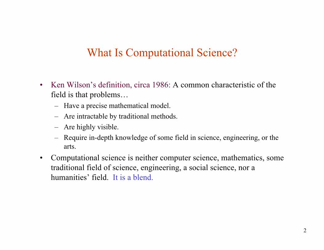
What Is Computational Science?
• Ken Wilson’s definition, circa 1986: A common characteristic of thefield is that problems…– Have a precise mathematical model.– Are intractable by traditional methods.– Are highly visible.– Require in-depth knowledge of some field in science, engineering, or the
arts.• Computational science is neither computer science, mathematics, some
traditional field of science, engineering, a social science, nor ahumanities’ field. It is a blend.
3
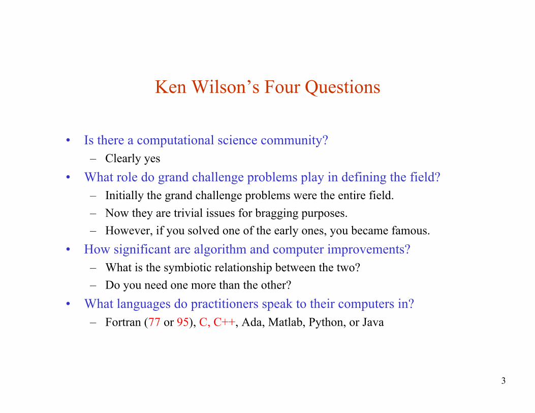
Ken Wilson’s Four Questions
• Is there a computational science community?– Clearly yes
• What role do grand challenge problems play in defining the field?– Initially the grand challenge problems were the entire field.– Now they are trivial issues for bragging purposes.– However, if you solved one of the early ones, you became famous.
• How significant are algorithm and computer improvements?– What is the symbiotic relationship between the two?– Do you need one more than the other?
• What languages do practitioners speak to their computers in?– Fortran (77 or 95), C, C++, Ada, Matlab, Python, or Java
4
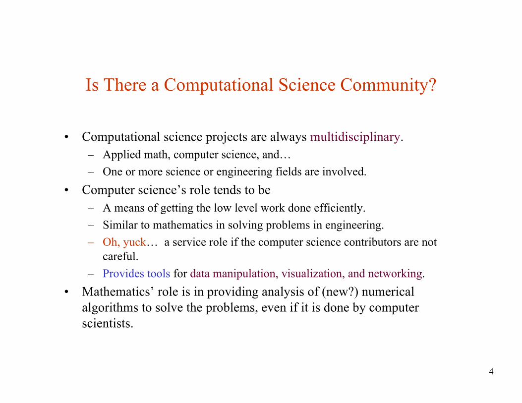
Is There a Computational Science Community?
• Computational science projects are always multidisciplinary.– Applied math, computer science, and…– One or more science or engineering fields are involved.
• Computer science’s role tends to be– A means of getting the low level work done efficiently.– Similar to mathematics in solving problems in engineering.– Oh, yuck… a service role if the computer science contributors are not
careful.– Provides tools for data manipulation, visualization, and networking.
• Mathematics’ role is in providing analysis of (new?) numericalalgorithms to solve the problems, even if it is done by computerscientists.
5
New Field’s Responsibilities
• Computational science is still an evolving field– There is a common methodology that is used in many disparate problems.– Common tools will be useful to all of these related problems if the
common denominator can be found.• The field became unique when it solved some small collection of
problems for which there is clearly no other solution methodology.• The community is still trying to define the age old question, “What
defines a high quality result?” This is slowly being answered.• An education program must be devised. This, too, is being worked on.• Appropriate journals and conferences already exist and are being used
to guarantee that the field evolves.• Various government programs throughout the world are pushing the
field.
6
Grand Challenge Problems
• New fields historically come from breakthroughs in other fields thatresist change.
• Definition: Grand Challenges are fundamental problems in science andengineering with potentially broad social, political, economic, andscientific impact that can be advanced by applying high performancecomputing resources.
• Grand Challenges are dynamic, not static.• Grand Challenge problems early on helped in defining the field. There
is great resistance in mathematics and computer science to theseproblems. Typically, the problems are defined by pagans from appliedscience and engineering fields who do not provide sufficient applauseto the efforts of mathematicians and computer scientists. The pagansjust want to solve (ill posed) problems and move on.
7
Some Grand Challenge Areas• Combustion• Electronic structure of materials• Turbulence• Genome sequencing and structural biology• Climate modeling
– Ocean modeling– Atmospheric modeling– Coupling the two
• Astrophysics• Speech and language recognition• Pharmaceutical designs• Pollution tracking• Oil and gas reservoir modeling• Model entire Internet
8
A Grand Challenge Example
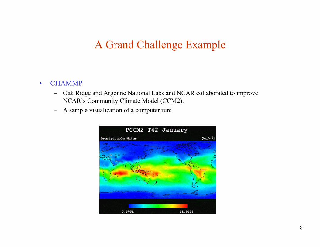
• CHAMMP– Oak Ridge and Argonne National Labs and NCAR collaborated to improve
NCAR’s Community Climate Model (CCM2).– A sample visualization of a computer run:
9
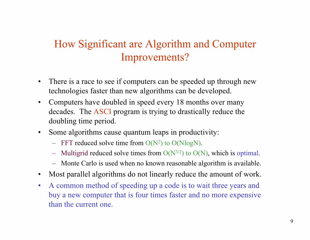
How Significant are Algorithm and ComputerImprovements?
• There is a race to see if computers can be speeded up through newtechnologies faster than new algorithms can be developed.
• Computers have doubled in speed every 18 months over manydecades. The ASCI program is trying to drastically reduce thedoubling time period.
• Some algorithms cause quantum leaps in productivity:– FFT reduced solve time from O(N2) to O(NlogN).– Multigrid reduced solve times from O(N3/2) to O(N), which is optimal.– Monte Carlo is used when no known reasonable algorithm is available.
• Most parallel algorithms do not linearly reduce the amount of work.• A common method of speeding up a code is to wait three years and
buy a new computer that is four times faster and no more expensivethan the current one.
10
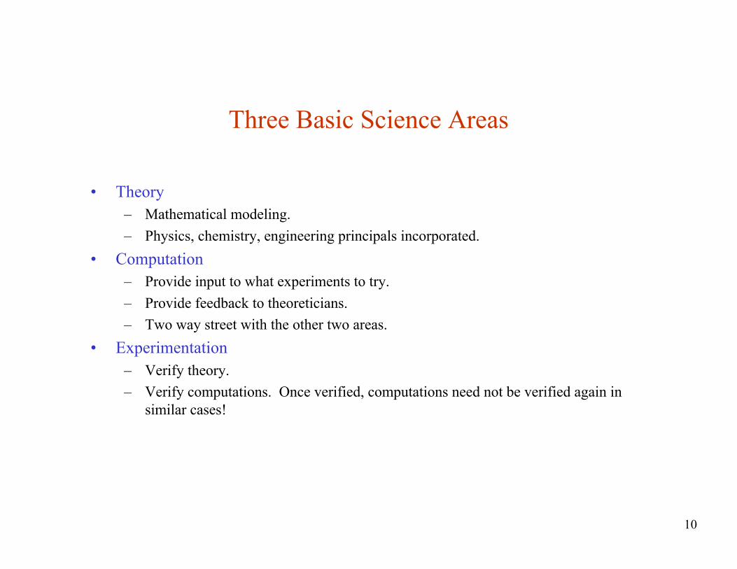
Three Basic Science Areas
• Theory– Mathematical modeling.– Physics, chemistry, engineering principals incorporated.
• Computation– Provide input to what experiments to try.– Provide feedback to theoreticians.– Two way street with the other two areas.
• Experimentation– Verify theory.– Verify computations. Once verified, computations need not be verified again in
similar cases!
11
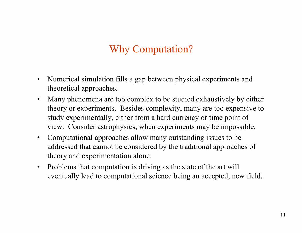
Why Computation?
• Numerical simulation fills a gap between physical experiments andtheoretical approaches.
• Many phenomena are too complex to be studied exhaustively by eithertheory or experiments. Besides complexity, many are too expensive tostudy experimentally, either from a hard currency or time point ofview. Consider astrophysics, when experiments may be impossible.
• Computational approaches allow many outstanding issues to beaddressed that cannot be considered by the traditional approaches oftheory and experimentation alone.
• Problems that computation is driving as the state of the art willeventually lead to computational science being an accepted, new field.
12
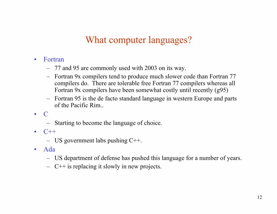
What computer languages?
• Fortran– 77 and 95 are commonly used with 2003 on its way.– Fortran 9x compilers tend to produce much slower code than Fortran 77
compilers do. There are tolerable free Fortran 77 compilers whereas allFortran 9x compilers have been somewhat costly until recently (g95)
– Fortran 95 is the de facto standard language in western Europe and partsof the Pacific Rim..
• C– Starting to become the language of choice.
• C++– US government labs pushing C++.
• Ada– US department of defense has pushed this language for a number of years.– C++ is replacing it slowly in new projects.
13
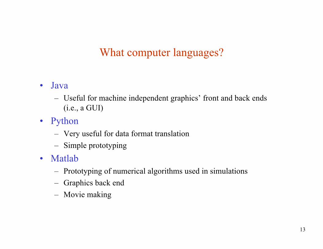
What computer languages?
• Java– Useful for machine independent graphics’ front and back ends
(i.e., a GUI)
• Python– Very useful for data format translation– Simple prototyping
• Matlab– Prototyping of numerical algorithms used in simulations– Graphics back end– Movie making
14
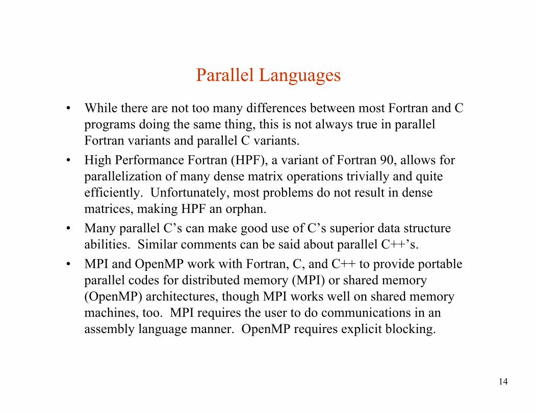
Parallel Languages• While there are not too many differences between most Fortran and C
programs doing the same thing, this is not always true in parallelFortran variants and parallel C variants.
• High Performance Fortran (HPF), a variant of Fortran 90, allows forparallelization of many dense matrix operations trivially and quiteefficiently. Unfortunately, most problems do not result in densematrices, making HPF an orphan.
• Many parallel C’s can make good use of C’s superior data structureabilities. Similar comments can be said about parallel C++’s.
• MPI and OpenMP work with Fortran, C, and C++ to provide portableparallel codes for distributed memory (MPI) or shared memory(OpenMP) architectures, though MPI works well on shared memorymachines, too. MPI requires the user to do communications in anassembly language manner. OpenMP requires explicit blocking.
15
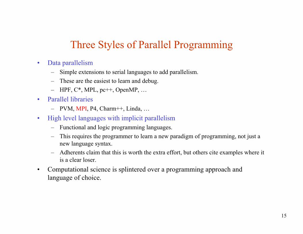
Three Styles of Parallel Programming• Data parallelism
– Simple extensions to serial languages to add parallelism.– These are the easiest to learn and debug.– HPF, C*, MPL, pc++, OpenMP, …
• Parallel libraries– PVM, MPI, P4, Charm++, Linda, …
• High level languages with implicit parallelism– Functional and logic programming languages.– This requires the programmer to learn a new paradigm of programming, not just a
new language syntax.– Adherents claim that this is worth the extra effort, but others cite examples where it
is a clear loser.• Computational science is splintered over a programming approach and
language of choice.
16
Computational Science Applications
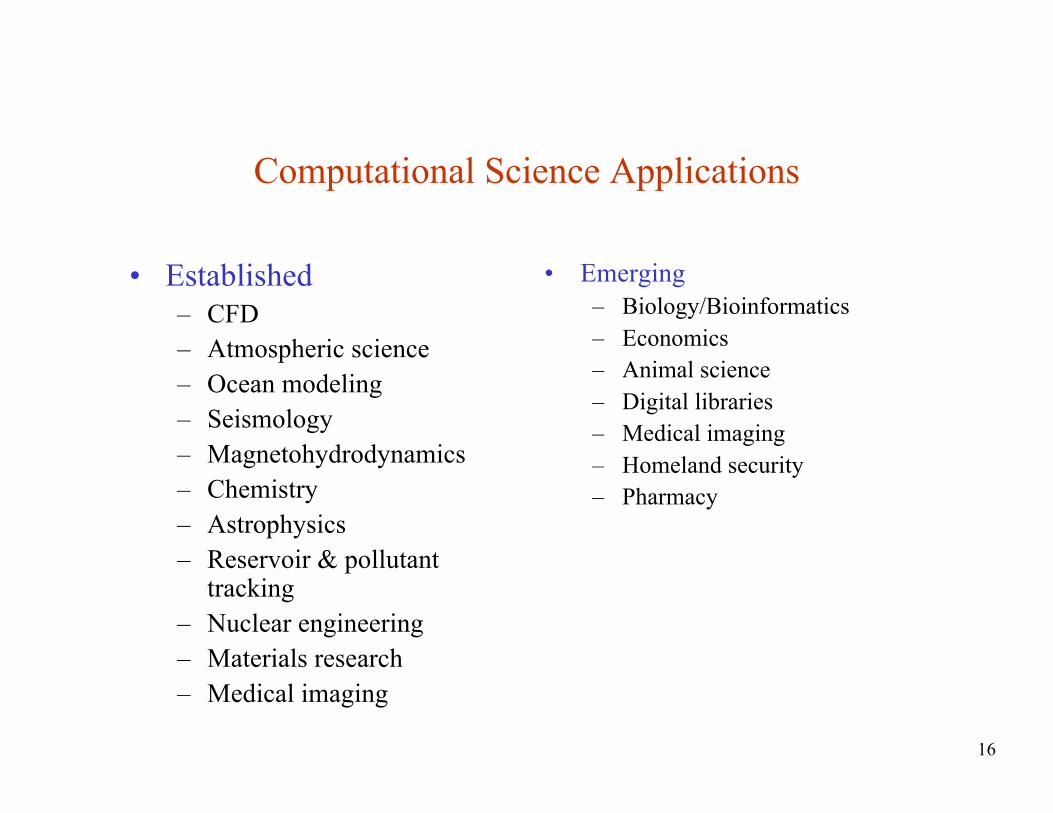
• Established– CFD– Atmospheric science– Ocean modeling– Seismology– Magnetohydrodynamics– Chemistry– Astrophysics– Reservoir & pollutant
tracking– Nuclear engineering– Materials research– Medical imaging
• Emerging– Biology/Bioinformatics– Economics– Animal science– Digital libraries– Medical imaging– Homeland security– Pharmacy
17
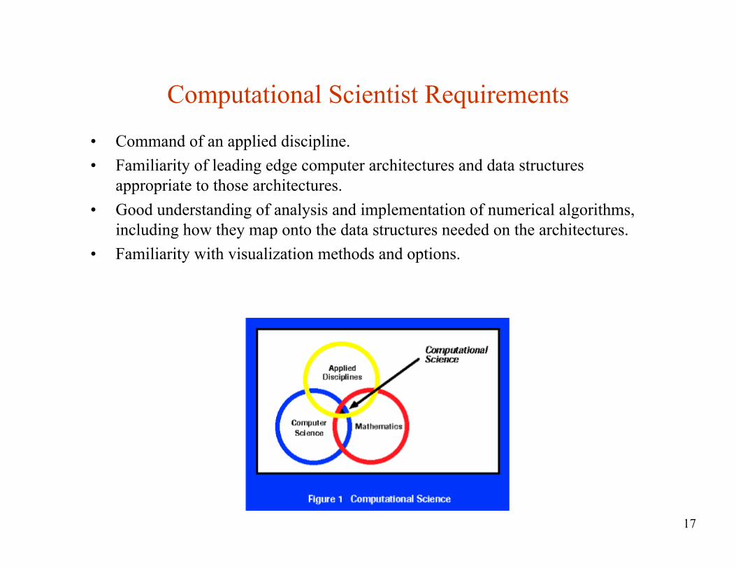
Computational Scientist Requirements
• Command of an applied discipline.• Familiarity of leading edge computer architectures and data structures
appropriate to those architectures.• Good understanding of analysis and implementation of numerical algorithms,
including how they map onto the data structures needed on the architectures.• Familiarity with visualization methods and options.
18
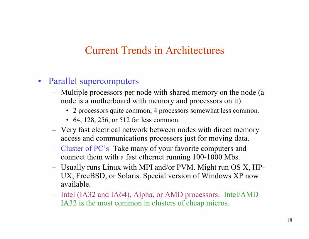
Current Trends in Architectures
• Parallel supercomputers– Multiple processors per node with shared memory on the node (a
node is a motherboard with memory and processors on it).• 2 processors quite common, 4 processors somewhat less common.• 64, 128, 256, or 512 far less common.
– Very fast electrical network between nodes with direct memoryaccess and communications processors just for moving data.
– Cluster of PC’s Take many of your favorite computers andconnect them with a fast ethernet running 100-1000 Mbs.
– Usually runs Linux with MPI and/or PVM. Might run OS X, HP-UX, FreeBSD, or Solaris. Special version of Windows XP nowavailable.
– Intel (IA32 and IA64), Alpha, or AMD processors. Intel/AMDIA32 is the most common in clusters of cheap micros.
19
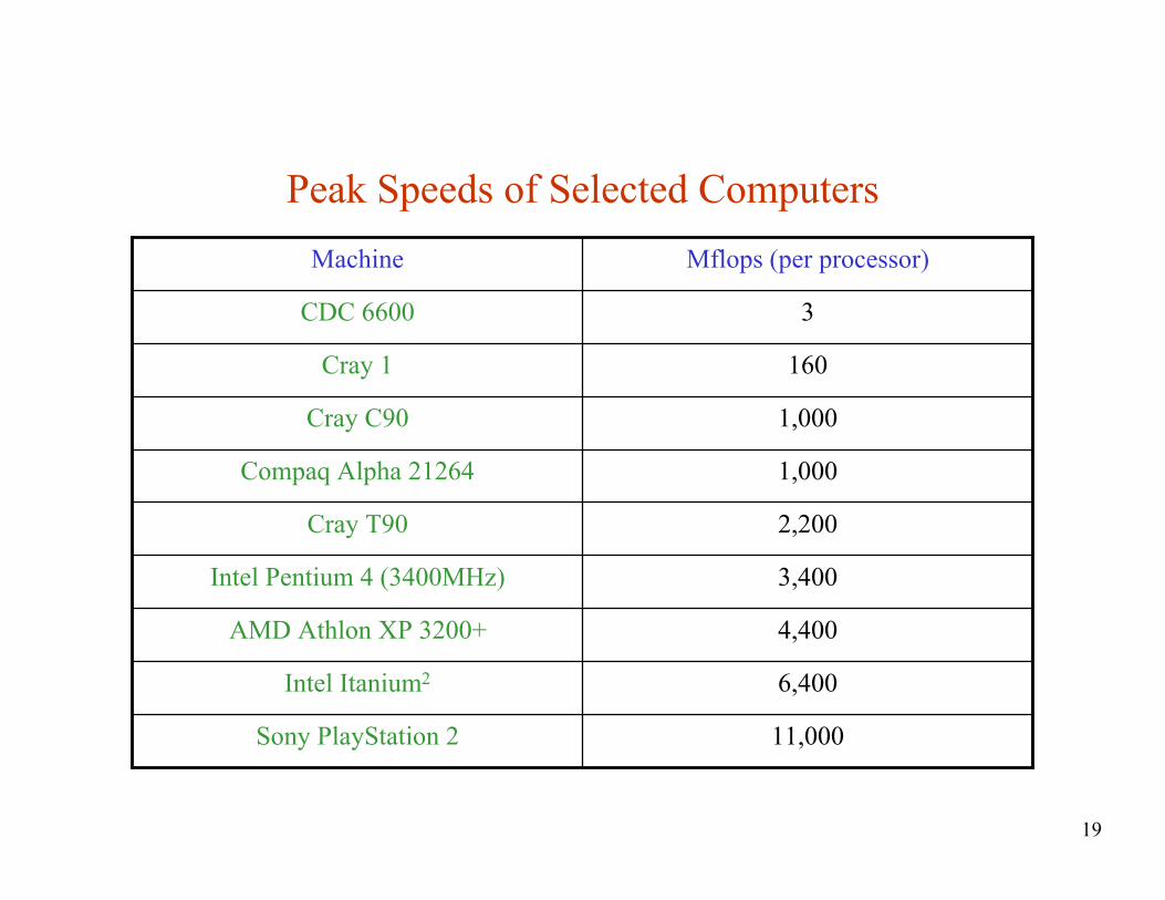
Peak Speeds of Selected Computers
4,400AMD Athlon XP 3200+
3,400Intel Pentium 4 (3400MHz)
11,000Sony PlayStation 2
1,000Compaq Alpha 21264
6,400Intel Itanium2
2,200Cray T90
1,000Cray C90
160Cray 1
3CDC 6600
Mflops (per processor)Machine
20
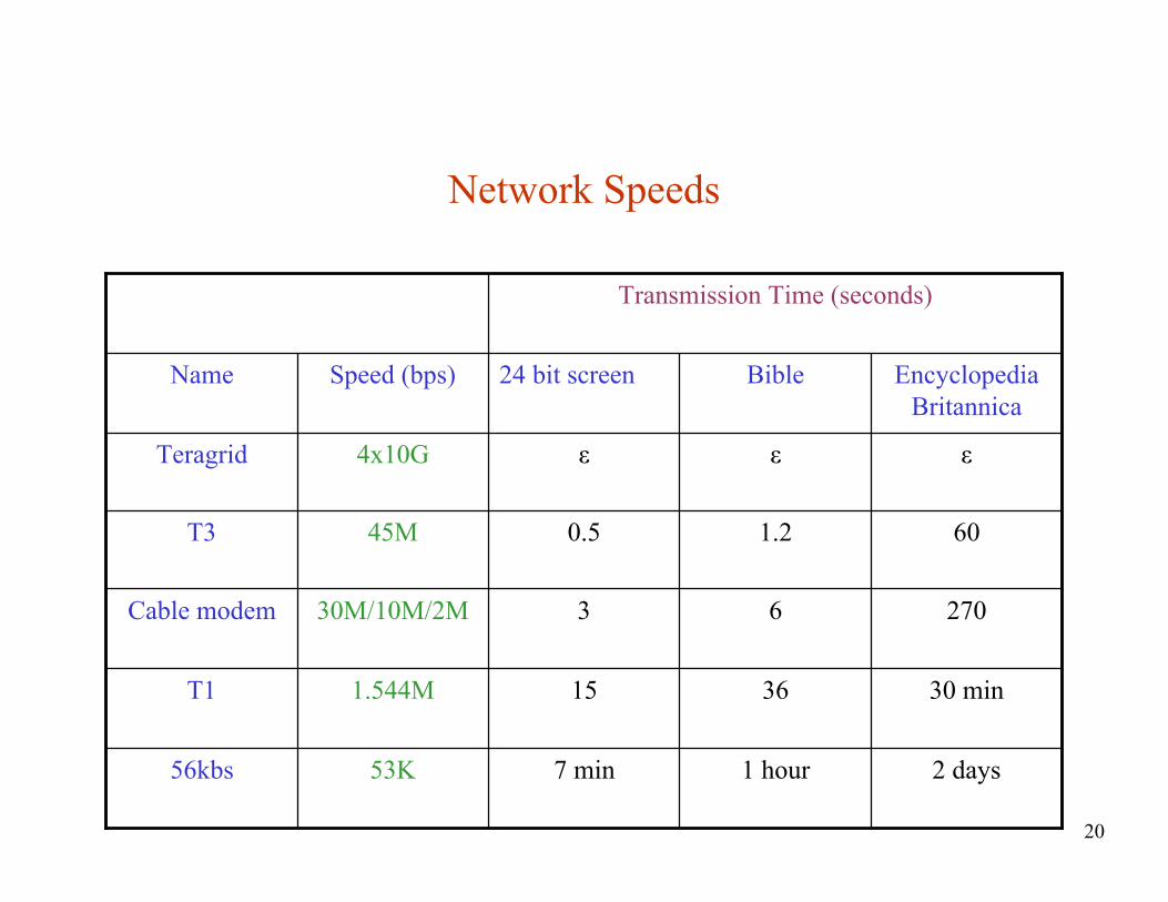
Network Speeds
εεε4x10GTeragrid
2 days1 hour7 min53K56kbs
30 min36151.544MT1
2706330M/10M/2MCable modem
601.20.545MT3
EncyclopediaBritannica
Bible24 bit screenSpeed (bps)Name
Transmission Time (seconds)
21
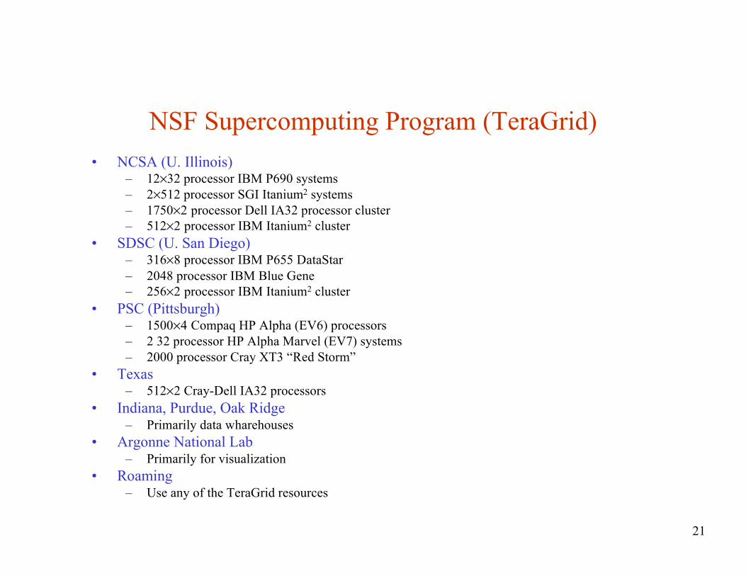
NSF Supercomputing Program (TeraGrid)• NCSA (U. Illinois)
– 12×32 processor IBM P690 systems– 2×512 processor SGI Itanium2 systems– 1750×2 processor Dell IA32 processor cluster– 512×2 processor IBM Itanium2 cluster
• SDSC (U. San Diego)– 316×8 processor IBM P655 DataStar– 2048 processor IBM Blue Gene– 256×2 processor IBM Itanium2 cluster
• PSC (Pittsburgh)– 1500×4 Compaq HP Alpha (EV6) processors– 2 32 processor HP Alpha Marvel (EV7) systems– 2000 processor Cray XT3 “Red Storm”
• Texas– 512×2 Cray-Dell IA32 processors
• Indiana, Purdue, Oak Ridge– Primarily data wharehouses
• Argonne National Lab– Primarily for visualization
• Roaming– Use any of the TeraGrid resources
22
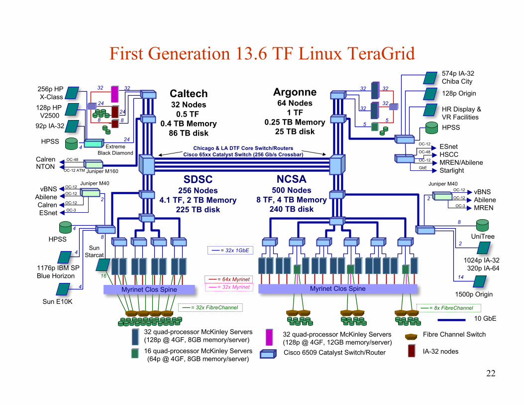
First Generation 13.6 TF Linux TeraGrid
32
32
5
32
32
5
Cisco 6509 Catalyst Switch/Router
32 quad-processor McKinley Servers(128p @ 4GF, 8GB memory/server)
Fibre Channel Switch
HPSS
HPSS
ESnetHSCCMREN/AbileneStarlight
10 GbE
16 quad-processor McKinley Servers(64p @ 4GF, 8GB memory/server)
NCSA500 Nodes
8 TF, 4 TB Memory240 TB disk
SDSC256 Nodes
4.1 TF, 2 TB Memory225 TB disk
Caltech32 Nodes
0.5 TF 0.4 TB Memory
86 TB disk
Argonne64 Nodes
1 TF0.25 TB Memory
25 TB disk
IA-32 nodes
4
Juniper M160
OC-12
OC-48
OC-12
574p IA-32Chiba City
128p Origin
HR Display &VR Facilities
= 32x 1GbE
= 64x Myrinet
= 32x FibreChannel
Myrinet Clos Spine Myrinet Clos Spine
Chicago & LA DTF Core Switch/RoutersCisco 65xx Catalyst Switch (256 Gb/s Crossbar)
= 8x FibreChannel
OC-12
OC-12
OC-3
vBNSAbileneMREN
Juniper M40
1176p IBM SPBlue Horizon
OC-48
NTON
32
248
32
24
8
4
4
Sun E10K
41500p Origin
UniTree
1024p IA-32 320p IA-64
2
14
8
Juniper M40vBNS
AbileneCalrenESnet
OC-12
OC-12
OC-12
OC-3
8
SunStarcat
16
GbE
= 32x Myrinet
HPSS
256p HP X-Class
128p HP V2500
92p IA-32
24Extreme
Black Diamond
32 quad-processor McKinley Servers(128p @ 4GF, 12GB memory/server)
OC-12 ATM
Calren
2 2