An Overview of Collaborative the Future Electric Energy...
14
An Overview of Collaborative Testbeds Within the Future Renewable Electric Energy Delivery and Management Center 1
Transcript of An Overview of Collaborative the Future Electric Energy...

An Overview of Collaborative Testbeds Within the Future
Renewable Electric Energy Delivery and Management Center
1

FREEDM Center
2

GEH
3

Green Energy Hub
• The Green Energy Hub testbed is an integrated hardware system demonstration incorporating technologies from the Enabling Technology and Fundamental Science research planes.
• Functions include testing and demonstration of– Solid State Transformer ‐ SST (Gen I, Gen II)– Fault Isolation Device ‐ FID (Gen I, Gen II)– Distributed Energy Storage Device – DESD (AC and DC)– Distributed Renewable Energy Resource ‐ DRER (PV, Wind)– Household Load Emulator
• Previous focus on basic power (Intelligent Power Management ‐ IPM) and fault management (Intelligent Fault Management ‐ IFM) functions.
4
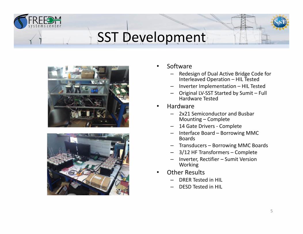
SST Development
• Software– Redesign of Dual Active Bridge Code for
Interleaved Operation – HIL Tested– Inverter Implementation – HIL Tested– Original LV‐SST Started by Sumit – Full
Hardware Tested• Hardware
– 2x21 Semiconductor and BusbarMounting – Complete
– 14 Gate Drivers ‐ Complete– Interface Board – Borrowing MMC
Boards– Transducers – Borrowing MMC Boards– 3/12 HF Transformers – Complete– Inverter, Rectifier – Sumit Version
Working• Other Results
– DRER Tested in HIL– DESD Tested in HIL
5

Hardware in the Loop Testbed
6

HIL
• HIL experiments with 10 kW Gen‐II SST at FSU‐CAPS– Setup will also incorporate DESD interface developed under DESD sub‐thrust (Dr. Li)
• Implement and test invariants for Multi‐Domain Cyber‐Physical Systems control in the HIL‐TB real‐time environment
• Implement and test DGI algorithms with Cyber‐Physical Security– Develop and test new security association (SA) mechanisms, and demonstrate the Ipsecbased
security platform using OPNET network emulator on the HIL‐TB• RTDS SST Model Validation
– Will validate switching and average models of SSTs used in HIL‐TB through correlation with test results from Gen‐II SST hardware
• Advanced Controller Validation– Implement robust control laws partly developed in Y6 (impedance uncertainty) and new
robust control laws to be developed in Y7 as part of SMC project (communication uncertainty) in the DSP/FPGA controller board used for SST CHIL on HIL‐TB
• Model Maintenance– Develop, maintain, and version control SST simulation model library; ensure compatibility with
the analytical models delivered to SMC– Engage with the FREEDM Architecture Working Group (FAWG)
7
LSSS
8
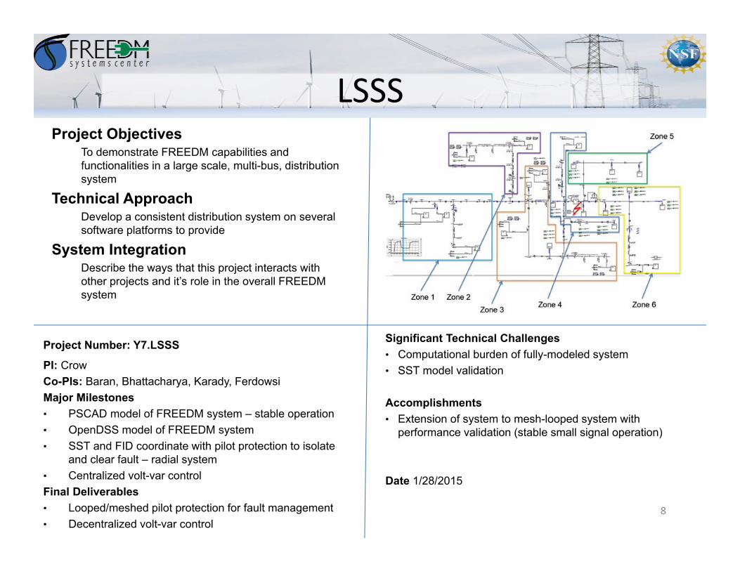
Project ObjectivesTo demonstrate FREEDM capabilities and functionalities in a large scale, multi-bus, distribution system
Technical ApproachDevelop a consistent distribution system on several software platforms to provide
System IntegrationDescribe the ways that this project interacts with other projects and it’s role in the overall FREEDM system
Significant Technical Challenges• Computational burden of fully-modeled system• SST model validation
Accomplishments• Extension of system to mesh-looped system with
performance validation (stable small signal operation)
Date 1/28/2015
Project Number: Y7.LSSS
PI: CrowCo-PIs: Baran, Bhattacharya, Karady, FerdowsiMajor Milestones• PSCAD model of FREEDM system – stable operation• OpenDSS model of FREEDM system• SST and FID coordinate with pilot protection to isolate
and clear fault – radial system• Centralized volt-var controlFinal Deliverables• Looped/meshed pilot protection for fault management• Decentralized volt-var control

Background/Motivation
The ultimate customer of the FREEDM system are utilities. Utilities will not adopt the SST and FID until they can be assured that• The SSTs and FIDs will not
interact poorly• System stability will be
maintained• System reliability and
resiliency will be improved (benefit > cost)
The LSSS is the demonstration platform that will provide the evidence of SST and FID operation in a distribution system
9
V Ph
12.47, 60.0 [Hz]12.0 [MVA]
0.0*
12.47
300 300 300
303
300 300 301 301
302
301 303
301
301 301 303
301301
301
301 301
301301
301 301
301 301
301
304
#1 #2
500 [kVA]12.47 [kV] / 4.16 [kV]
300
A B C
0.19
2333
[ohm
]0.
2707
5 [m
H]
3.08 [nF]
0.22
6675
[ohm
]0.3
25 [m
H]
302
1.59
5595
75 [o
hm]2
.245
75 [m
H]
302
1.36594925 [ohm]1.9225 [mH]
0.10040825 [ohm]141.25 [uH]
1.608 [nF]
0.77311 [ohm] 1.08825 [mH]
12.38 [nF]
0.36055225 [ohm]
216.75 [uH]
302
0.05
3683
5 [o
hm]7
5.5
[uH
]
0.86 [nF]
BUS846
BUS828
BUS824BUS816
BUS850
BUS818
BUS822
BUS800 BUS802 BUS806 BUS808 BUS812 BUS814
BUS830BUS854
BUS852
BUS858
BUS832
BUS844
BUS842
BUS848
BUS834BUS860
BUS836
BUS840
BUS862
BUS888
BUS890
BUS826
Ps
Qs
0.57
6999
25 [o
hm]
0.81
225
[mH
]
9.24 [nF]
BUS810
4.78
6787
5 [o
hm]
6.73
75 [m
H]
BUS8200.4553165 [ohm]0.64075 [mH]
0.30
1224
5 [o
hm]0.
424
[mH
]
4.824 [nF]
2.31933 [ohm] 3.2645 [mH]
37.14 [nF]
BUS856
0.16
105
[ohm
]226
.75
[uH
]
2.579 [nF]
BUS864
0.081657 [ohm]
0.6505 [mH
]
BUS838
P = 0.01551Q
= -0.0001993V = 0.9791
V A
P =
0.17
03Q
= -0
.001
093
V =
0.91
67
VA
P =
0.17
02Q
= -0
.001
092
V =
0.91
59
VA
P = 0.1328Q = -0.002456
V = 0.8932
VA
P = 0.003866Q = -0.0008682
V = 0.9138
VA
P =
0.00
194
Q =
-0.0
0013
17V
= 0.
8596
VA
V =
0.97
88
VA
P = 0.1321Q = -0.001661
V = 0.888
VA
V =
0.93
25
VA
V =
0.85
96
VA
V = 0.8755
V A
PQ PQ
P = 5.929Q = 0.1502
V = 1
VA
PQ PQ PQ
PQ
PQ
PQ
PQ
PQ
PQ PQ
PQ
PQ
PQ
Main ...
1.2
0
Vs
1
IEEE 34 BUS DISTRIBUTION TEST MODELDeveloped June 2006by Jen Z. Zhou, Dharshana Muthumuni, and Paul WilsonThis version has no wind generators and can only run in professional version of PSCAD.
IEEE Description papers and discussion available.
Q = -0.0001951V = 0.9136
VA
Ea
Eb
Ec
Ec
Eb
Ea
Main : Graphs
x 2.580 2.590 2.600 2.610 2.620 2.630 2.640 2.650 2.660
-12.5
-10.0
-7.5
-5.0
-2.5
0.0
2.5 5.0
7.5
10.0
(kA)
I890 I890 I890
0.007991 [uF]
2.664 [nF]
3.6 [nF]
25.55 [nF]
76.65 [nF]
7.291 [nF]
21.873 [nF]
Main : Graphs
x 0.0 1.0 2.0 3.0 4.0 5.0 6.0
-1.0
0.0
1.0
2.0
3.0
4.0
5.0
6.0
(MW
)
Ps
A
B
CBRK1
BRK2
TimedBreakerLogic
Open@t0BRK1
TimedBreakerLogic
Closed@t0
BRK2
BRK3
BRK4Timed
BreakerLogic
Closed@t0BRK3
TimedBreakerLogic
Open@t0BRK4
BRK5
A
B
C
BRK6
BRK6
TimedBreakerLogic
Open@t0BRK5
TimedBreakerLogic
Closed@t0
BRK8
BRK7A
B
C TimedBreakerLogic
Closed@t0BRK7
TimedBreakerLogic
Open@t0BRK8
A
B
C
BRK9
BRK10
BRK10
TimedBreakerLogic
Open@t0BRK9
TimedBreakerLogic
Closed@t0
SST824
Tabc
A
B
CBRK13
BRK14
BRK14
TimedBreakerLogic
Open@t0BRK13
TimedBreakerLogic
Closed@t0
BRK16
BRK15
A
B
C
TimedBreakerLogic
Closed@t0BRK15
TimedBreakerLogic
Open@t0BRK16
SST830
Tabc
A
B
CBRK23
BRK24
BRK24
TimedBreakerLogic
Open@t0BRK23
TimedBreakerLogic
Closed@t0
SST858
Tabc
BRK38
BRK38
TimedBreakerLogic
Open@t0BRK37
TimedBreakerLogic
Closed@t0
A
B
C
BRK37
SST834
Tabc
SST860
Tabc
SST836
Tabc
SST840
Tabc
BRK63
A
B
C
BRK64
TimedBreakerLogic
Closed@t0BRK63
TimedBreakerLogic
Open@t0BRK64
SST844
Tabc
SST846
Tabc
SST848
Tabc
SST890
Tabc
SST
Q806B0.0Q806B
SST
0.0Q806C
Q806C
SST
Q810B0.0Q810B
SST
0.0Q820A
Q820A
SST
Q822A0.0Q822A
Q824B0.0Q824B
0.0Q826B
Q826B
SST
SST
0.0Q828C
Q828C 0.0Q830A
Q830A
0.0Q830B
Q830B
0.0Q830C
Q830C
Q856B0.0Q856B
SST
Q890C0.0Q890C
Q890B0.0Q890B
Q890A0.0Q890A
0.0Q858A
Q858A
0.0Q858B
Q858B
0.0Q858C
Q858C
SST
Q864A0.0Q864A
0.0Q834A
Q834A
0.0Q834B
Q834B
0.0Q834C
Q834C
Q860C0.0Q860C
Q860B0.0Q860B
Q860A0.0Q860A
Q836C0.0Q836C
Q836B0.0Q836B
Q836A0.0Q836A
0.0Q838B
Q838B
SST
0.0Q844A
Q844A
0.0Q844B
Q844B
0.0Q844C
Q844C
Q846C0.0Q846C
Q846B0.0Q846B
Q848C0.0Q848C
Q848B0.0Q848B
Q848A0.0Q848A
6.9807e-4 [H]0.089179 [ohm]
feeder3
feeder17.8532e-4 [H]
0.1003 [ohm]
5.2356e-4 [H]
0.066948 [ohm]
SST
Tabc
SST
Tabc
6.9807e-4 [H]
0.066948 [ohm]
5.2356e-4 [H]
6.9807e-4 [H]
SST
Tabc
SST
Tabc
feeder3
7.8532e-4 [H]0.1003 [ohm]
5.2356e-4 [H]
0.066948 [ohm]
SST
Tabc
0.066948 [ohm]
5.2356e-4 [H]
0.1003 [ohm]
7.8532e-4 [H]
feeder1
feeder3
6.9807e-4 [H]
SST
Tabc
SST
Tabc
0.089179 [ohm]
0.089179 [ohm]
0.089179 [ohm]
feeder2 feeder2 feeder2
feeder1
feeder1
feeder2
Q1C0.0
Q1B0.0
Q1A0.0 0.0 Q2A
0.0 Q2B
0.0 Q2C Q3C0.0
Q3B0.0
Q3A0.0
Q4C0.0
Q4B0.0
Q4A0.0 0.0 Q5A
0.0 Q5B
0.0 Q5C Q6C0.0
Q6B0.0
Q6A0.0
Q7C0.0
Q7B0.0
Q7A0.0
BRKcon1
BRKcon2
TimedBreakerLogic
Open@t0 BRKcon1
TimedBreakerLogic
Open@t0 BRKcon2

Example Project 1Pilot directional protection
10
Unsymmetrical faults
• For a fault at the given location, R1, R2 and R3 calculate the direction of fault currents. The directionality offault current is communicated between the relays R1, R2 and R2, R3.
• Since R1 and R2 have the same direction of fault current, fault is not located in between them. R2 and R3have different fault current directions. Hence fault location is in between them.
Relay Faultdirection
Relay Fault direction
R1 Forward R2 ForwardR2 Forward R3 ReverseTrip signal No trip Trip signal Trip generated
Fault is between relay 1 and relay 2
Green signal is +1 Forward fault for relay 1Red signal is ‐1 Reverse fault for relay 2

11
Example Project 1
Remaind
er of system
Fault Interruption Device (FID)

Example Project 1
12
SST838B : SST Output
x 0.0 1.0 2.0 3.0 4.0 5.0 6.0 7.0
-300
-200
-100
0
100
200
300
y
Vhs
-30
-20
-10
0
10
20
30
y
Ipl
-300
-200
-100
0
100
200
300
y
Vnl
-30
-20
-10
0
10
20
30
y
Inl
SST Waveforms
x 0.0 1.0 2.0 3.0 4.0 5.0 6.0 7.0
-10.0k
-5.0k
0.0
5.0k
10.0k
Inpu
t Vol
tage
Vhs
-30
-20
-10
0
10
20
30
Inpu
t Cur
rent
Ihs
3.4k3.6k3.8k4.0k4.2k4.4k4.6k4.8k
HVD
C C
apac
itor V
olta
ge
Vhdc
399.70
399.80
399.90
400.00
400.10
400.20
LVD
C C
apac
itor V
olta
ge
Vldc
SST response outside of Fault RegionSST response inside of Fault Region

13
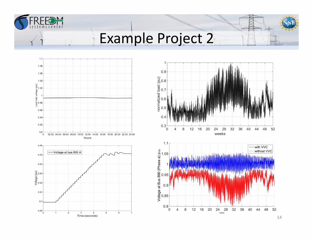
Example Project 2Distributed Volt‐Var Control
Non‐VVC SSTs hold unity pf
Actual solar insolation
Example Project 2
14
![PMU Placement to Ensure Observable Freqqyuency and Voltage Dynamics…electriconf/2012/slides/Section D2-P1/2... · References [1] Ali Abur, Optimal Plancement of Phasor Measurement](https://static.fdocuments.in/doc/165x107/5a827d217f8b9ada388de528/pmu-placement-to-ensure-observable-freqqyuency-and-voltage-dynamics-electriconf2012slidessection.jpg)