An overview of cloud and precipitation microphysics and its parameterization in

models

Hugh Morrison

NCAR*Mesoscale and Microscale Meteorology Division, NESL

WRF Workshop, June 21, 2010

*National Center for Atmospheric Research is

sponsored by the National Science Foundation

Outline

• Background/introduction

• Basics of microphysics parameterization- Liquid schemes

- Ice microphysics and mixed-phase schemes

- Multi-moment schemes

• Microphysics and data assimilation

• General thoughts on use of microphysics

schemes

Cloud particles (microphysics) Individual clouds

0.5 mm

Mesoscale cloud systemsWeather systems

1000 km

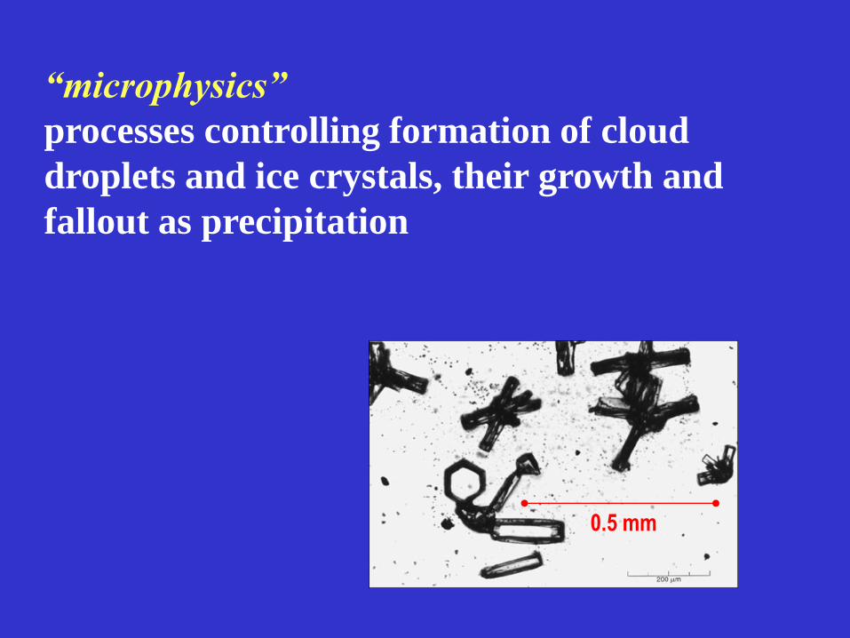
“microphysics”

processes controlling formation of cloud

droplets and ice crystals, their growth and

fallout as precipitation

0.5 mm

“microphysics parameterization”

“parameterization”

grid-scale microphysics

Predicted temperature,

moisture, wind, etc.

latent heating,

drying/moistening

“macrophysics” schemes are often used in

larger-scale models (cloud fraction, PDF cloud

schemes) to drive microphysics

Microphysics plays a key role in cloud, climate and weather models

Stephens (2005)-Latent heating/cooling(condensation, evaporation, deposition,

sublimation, freezing, melting)

-Condensate loading (mass of the condensate carried by the flow)

-Precipitation(fallout of larger particles)

-Coupling with surface processes (moist downdrafts leading to surface-wind

gustiness, cloud shading)

-Radiative transfer(mostly mass for absorption/emission of LW, particle size also important

for SW)

-Cloud-aerosol-precipitation interactions(aerosol affect clouds: indirect aerosol effects, but clouds process aerosols

as well)

Overview of microphysics

parameterization

Microphysics schemes can be broadly

categorized into two types:

N(D)

Diameter (D)

N(D)

Diameter (D)

Detailed (bin) bulk

Representation of particle size distribution

Size distribution

assumed to follow

functional form

Size distribution

discretized into

bins

Bulk schemes predict one or more bulk quantities

(e.g., mixing ratio) and assume some functional form

for the particle size distribution, e.g., gamma

distribution:

n(D) = N0 Dm e-lD

If N0 and m are specified, then l can be obtained from

the predicted mixing ratio q:

Equations for

isometric particle

shapes

Liquid microphysics – Kessler (1969)

• Separate liquid into cloud water and rain

N(D)

N(D)

N(D)

Droplet mass distribution

evolution during rain

formation using a detailed bin

model.

Grabowski and Wang 2009

Time

N(D)

Diameter (D)

N(D)

N(D)

Accretion of cloud water by existing rain

Autoconversion of cloud water to form rain

Diffusional growth of cloud water

• Key liquid microphysical conversion processes

Liquid microphysics – Kessler (1969)

• Separate liquid into cloud water and rain

• Marhsall-Palmer distribution for rain

qr

Rain

(Prognostic)

qc

CloudWater

(Prognostic)

qv

Water Vapor

(Prognostic)

Sedimentation

Autoconversion/

Accretion

Evaporation/

Condensation

Evaporation

Marshall-Palmer (1948) rain drop distribution

- N0 = 8 x 106 m-4

- m = 0

N(D)

Log Particle Diameter (D)

N0

Slope l

Extension to ice phase

…subsequent studies extended the Kessler

approach to include ice (e.g., Koenig and Murray

1976; Lin et al. 1983; Rutledge and Hobbs 1984; Lord et al.

1984; Dudhia 1989)

Ice microphysical processes

• Diffusional growth/sublimation

• Aggregation (autoconversion, accretion)

• Collection of rain and cloud water (riming)

• Melting

• Freezing

• Ice particle initiation (nucleation)

• Sedimentation

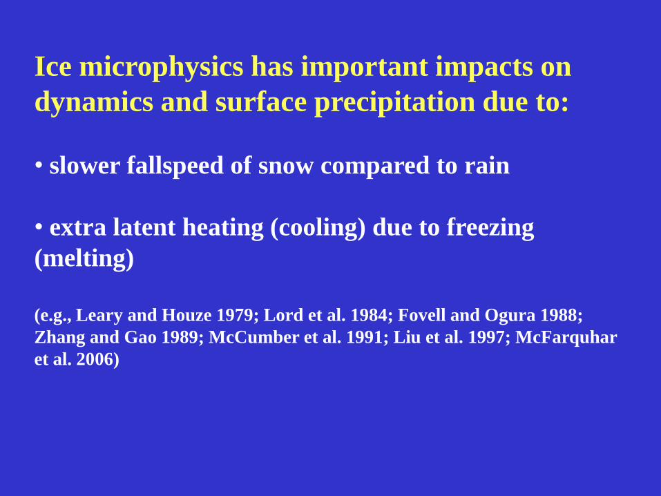
Ice microphysics has important impacts on

dynamics and surface precipitation due to:

• slower fallspeed of snow compared to rain

• extra latent heating (cooling) due to freezing

(melting)

(e.g., Leary and Houze 1979; Lord et al. 1984; Fovell and Ogura 1988;

Zhang and Gao 1989; McCumber et al. 1991; Liu et al. 1997; McFarquhar

et al. 2006)

Example: Impact of ice microphysics on 2D

tropical squall line

Liu et al. 1997

Liquid only (Kessler)

Ice + Liquid (Koenig and

Murray)

However, there is strong

case dependence of effects!

However, ice microphysics is significantly more

complicated because of the wide variety of ice

particle characteristics…

Pristine ice crystals,

grown by diffusion of

water vapor

Snowflakes, grown by

aggregation

Pruppacher and Klett

Rimed ice crystals

(accretion of supercooled

cloud drops)

Graupel (heavily rimed ice

crystals)

Hail

Different types of ice (small ice, snow, graupel, hail,

etc.) are typically parameterized by partitioning ice

into different species whose characteristics (N0,

particle density, fallspeed) are determined a priori.

• “Effective density” of ice particles is typically

expressed by a mass-size relationship of the form:

m = aDb

• In many schemes, b = 3 (corresponding with

spheres) and a ~ 0.1 g cm-3 (snow), ~ 0.4 g cm-3

(graupel), or ~ 0.9 g cm-3 (hail).

• More recently, schemes have been developed that

assume b ~ 2 (Thompson et al. 2008; Milbrandt et

al. 2010; Morrison and Grabowski 2008), which is

closer to observationally- and theoretically-derived

values.

Rutledge and Hobbs, JAS 1984

Different ice species have very different

characteristics!

Straka and Mansell (2005)

How ice is separated into different species

(cloud ice, snow, graupel, hail, etc.) can have a

large impact on simulations.

2D tropical squall line

simulations

McCumber et al. (1991)

Graupel

Hail

from Biggerstaff and Houze (1993)

3D mid-latitude squall line simulations

Morrison and Bryan (2010, in prep)

It seems likely that “optimal” parameterization settings in terms of number and type of ice species are case dependent. Even within a given species, there is large variability - in general the boundaries between different species are not obvious.

-

From A. Heymsfield

• Recent work has attempted to move away from the

paradigm of separating ice into different species w/

fixed characteristics, and instead allow particle type

to vary as a function of the rime and vapor deposition

ice mixing ratios or process rates, which are predicted

or diagnosed separately (Stoelenga et al. 2007;

Morrison and Grabowski 2008; Lin and Colle 2010).

-

• Vapor depositional

growth • Riming of crystal

interstices

• Vapor depositional growth

• Further growth by

riming and vapor

deposition

• Complete filling-in

of interstices with

rime

Stage 2: Partially-rimed crystalStage 1: Unrimed crystal Stage 3: Graupel

D

Morrison and Grabowski

2008

Multi-moment versus single-moment schemes

• Single-moment – predict mixing ratio only for each

species

• Multi-moment – predict additional quantities for

each species (number concentration, reflectivity)

Prediction of additional moments allows greater

flexibility in representing size distributions and

hence microphysical process rates.

N(D) = N0 Dm e-lD

• Prediction of 2nd moment (number concentration N)

allows N0 to vary with q and N, giving scheme more

flexibility (e.g., Koenig and Murray 1976; Ferrier 1994; Meyers et al.

1997; Seifert and Beheng 2001; Milbrand and Yau 2005; Morrison et al.

2005)

• Prediction of 3rd moment (reflectivity Z) allows N0

and m to vary with q, N, and Z (e.g., Milbrandt and Yau 2005;

Gilmore and Straka 2009)

Key impacts of single vs. double-moment:

• Sedimentation (treatment of size sorting)

• Evaporation of rain - 2-moment schemes have a more

flexible treatment of rain drop mean size

Example: Impact of single vs. double-moment

on idealized 2D squall lineMorrison et al. 2009

2-moment

1-moment

Precip

Reflectivity

t = 6 hr

Example: Impact of single vs. double-moment

on idealized 2D squall line

Small N0, low evaporation rate in 2-

moment simulationWeaker cold pool in 2-moment

simulation

Spatial structure of N0 in 2-moment scheme is consistent with observations

(e.g., Waldvogel 1974; Tokday and Short 1996).

Morrison et al. 2009

• Other parameters also impact rain drop size

distribution and hence evaporation rate (rain

drop breakup, rain size distribution width or

shape, etc.).

Example: parameterization of rain drop

breakup in simulations of tornadic

supercell thunderstorms, Dx = 1 km

Morrison and Milbrandt (2010)

Microphysics and data assimilation

• Assimilation of radar reflectivity, satellite radiances,

etc.- Requires reasonable level of complexity of microphysics for

forward operator to “correctly” partition increments

• Issues with development of tangent linear and

adjoint models for microphysics

- Nonlinearity of microphysics (e.g., rain evaporation)

- Complex interaction (e.g., 3-species interaction)

- Conditionals/branches (e.g., autoconversion thresholds)

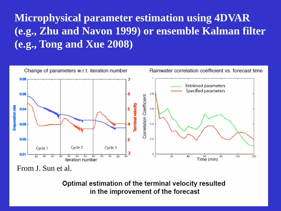
Microphysical parameter estimation using 4DVAR

(e.g., Zhu and Navon 1999) or ensemble Kalman filter

(e.g., Tong and Xue 2008)

From J. Sun et al.)

Key uncertainties – microphysical parameters

• Depends on type of microphysics scheme (number of

species and moments)

- One-moment schemes – N0 (but predicted in 2-moment

schemes…)

• Ice microphysics – density, fallspeed, etc.

• Conversion parameters – snow to graupel, liquid

and ice autoconversion, etc.

Case dependence of parameters??

Large uncertainties remain in our basic

understanding of the physical processes

of ice particles!

- Nucleation

- Particle shape (habit)

- Diffusional growth

- Aggregation, breakup

- Riming

General thoughts on the use of

microphysics schemes

How does one choose which type of microphysics scheme to use?

Many factors to consider:

Computational cost – number of species and predicted

moments is key (can be few % increase in run time with

each additional prognostic variable in WRF)

Appropriateness for application (e.g., real time forecasting

vs. research)

Appropriateness for case (liquid vs. mixed-phase, 3-

species ice vs. 2-species ice)

There has been a trend toward the use of more

complex microphysics schemes (i.e., more species

and more predicted moments) given:

- desire for better physical realism and representation of

microphysical processes

- need for more flexibility to cover a large number of

different applications

The development of more complex schemes has been

possible because of:

- increasing computer power

- improvements in understanding underlying physical

processes (theory and observations)

While more complex schemes improve physical

realism and are able to simulate microphysical

processes more realistically, they may not necessarily

lead to consistently better results (especially w/o

tuning).

- more realistic microphysics may expose other model deficiencies

(e.g., resolution, initialization/forcing, etc.)

- other physical parameterizations (e.g., PBL, radiation) have

often been developed and tuned to work with simpler

microphysics schemes

Differences are often as large or larger amongst

simulations using more complex schemes than

amongst those using simpler schemes, and while

complex schemes are useful as benchmarks for

testing simpler schemes, this should be done with

care.

- more degrees of freedom in complex schemes means divergence

of results is more likely

- key uncertainties related to the underlying physics often can’t be

addressed by increasing complexity of the scheme, and therefore

still require arbitrary or tuned parameter settings

Summary

• Microphysics parameterization is key in weather and climate

models because of interaction with dynamics, radiation,

aerosols/chemistry, etc.

• Microphysics parameterizations vary widely in complexity,

with a general trend toward use of more detailed multi-

moment and multi-species schemes.

• Numerous uncertainties remain in our understanding of the

basic physics, especially for the ice phase. Progress depends on

improvements in theory and especially observations (e.g., lab

studies).

Thank you!

Questions?