REVIEW ARTICLE

An optimisation approach for analysing nonlinear

stability with transition to turbulence in fluids as an

exemplar

R R Kerswell1, C C T Pringle2 and A P Willis3

1 School of Mathematics, University of Bristol, Bristol BS8 1TW, UK2 Applied Mathematics Research Centre, Faculty of Engineering and Computing,

Coventry University, Coventry CV1 5FB, UK3 School of Mathematics and Statistics, University of Sheffield, Sheffield S3 7RH, UK

E-mail: R.R.Kerswell@bris.ac.uk

Abstract.

This article introduces and reviews recent work using a simple optimisation

technique for analysing the nonlinear stability of a state in a dynamical system. The

technique can be used to identify the most efficient way to disturb a system such

that it transits from one stable state to another. The key idea is introduced within

the framework of a finite-dimensional set of ordinary differential equations (ODEs)

and then illustrated for a very simple system of 2 ODEs which possesses bistability.

Then the transition to turbulence problem in fluid mechanics is used to show how

the technique can be formulated for a spatially-extended system described by a set

of partial differential equations (the well-known Navier-Stokes equations). Within

that context, the optimisation technique bridges the gap between (linear) optimal

perturbation theory and the (nonlinear) dynamical systems approach to fluid flows.

The fact that the technique has now been recently shown to work in this very high

dimensional setting augurs well for its utility in other physical systems.

PACS numbers:

2

1. Introduction

Many physical systems possess a multiplicity of stable states so that more than one

solution or system configuration can be found at long times. In such situations, a

key issue is usually maintaining the system in a desired state against ambient noise or

switching the system from one (undesirable) state to another (preferred) state in an

efficient, robust way: e.g. in liquid crystal displays [76], power grids [84], arrays of

coupled lasers [41], turbulent fluid flows [51] and even in the human brain [3]. Either

objective involves detailed knowledge of a state’s basin of attraction, defined as the

set of all initial conditions of the system whose long time behaviour is to converge to

that state. Initial conditions located just outside the basin boundary indicate how the

system can be efficiently disturbed to trigger a new stable state. Knowledge of how

the basin boundary of a state moves (in phase space) when the system is manipulated

(e.g. by modifying the boundary conditions) opens up the possibility of enhancing the

nonlinear stability of that state to finite amplitude disturbances. However, locating a

basin boundary is a fully nonlinear (nonlocal) problem so that the traditional tools of

linearising the system around the state or even weakly nonlinear analysis provide no

traction. Existing fully nonlinear approaches - solving the governing equations while

searching for the finite-amplitude disturbances to just knock the system out of one state

into another, or mapping out the stable and unstable manifolds of nearby solutions in

phase space to identify the basin boundary - are impractical for all but the smallest

systems.

Recently, a new, very general, fully nonlinear optimisation technique has emerged

as a viable way to make progress. The underlying idea is relatively simple and, perhaps

because of this, seems to have been formulated independently in (at least) three different

parts of the scientific literature over the last decade (transitional shear flows [18, 86, 104]

- see §3, oceanography [89] - see §4.1 and thermoacoustics [69] - see §4.2). The key

advance, however, has come in the last few years when the feasibility of the approach

has been demonstrated for the 3-dimensional Navier-Stokes equations discretised by a

large number (O(105-106)) of degrees of freedom [18, 19, 21, 37, 86, 104, 105, 108]. This

suggests that other partial differential equation systems could be usefully analysed with

this approach.

This article (which is an updated and extended version of [74]) is an attempt to

provide a simple introduction to the idea and to review the progress made so far.

As should become clear, the approach is still developing but there is already enough

evidence garnered to indicate that it adds something quite new to a theoretician’s

toolbox. In fluid mechanics, the last two decades have seen a huge amount of work

looking at flow transition either from the linear transient growth perspective (also

called ‘non-modal analysis’ or ‘optimal perturbation theory’ [54, 113, 117, 116]) or

more recently in terms of exact solutions and their manifolds (a dynamical systems

approach [73, 39, 72]). The optimisation technique discussed here bridges the well-

known ‘amplitude’ gap between these two viewpoints by extending the (infinitesimal

3

amplitude) transient growth optimal of the former approach into finite amplitudes and

ultimately up to where the basin boundary is crossed (the closest stable manifold of a

nearby exact solution).

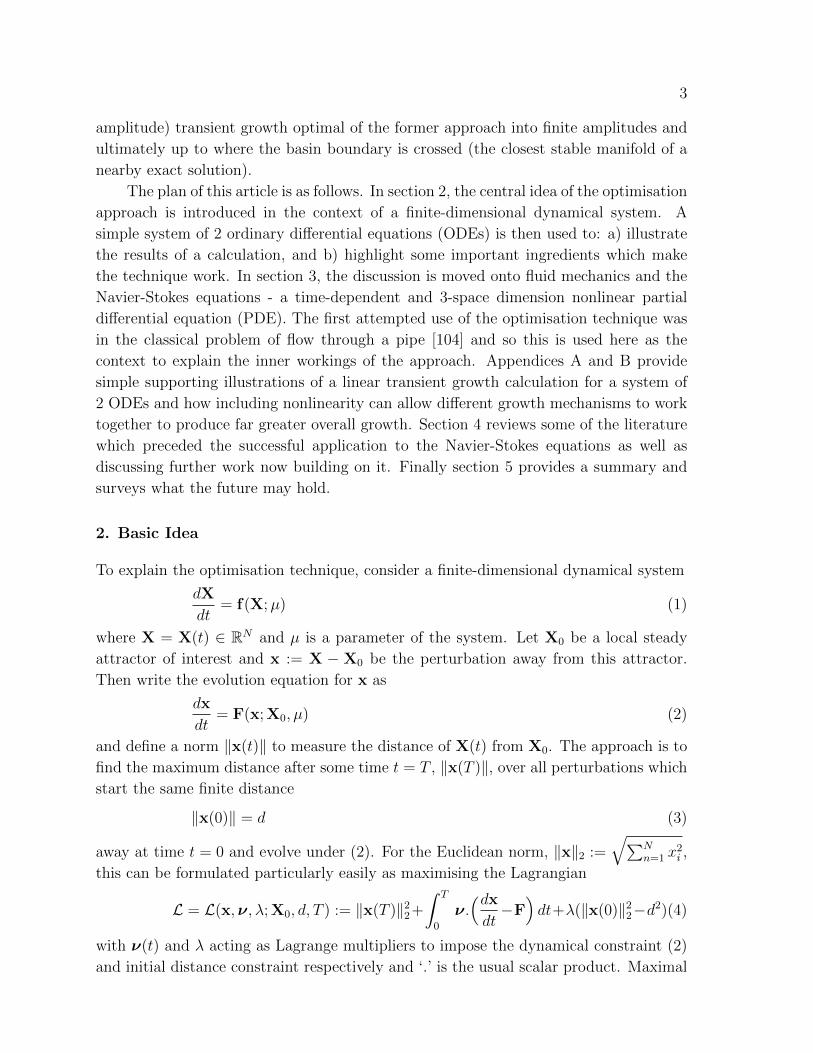
The plan of this article is as follows. In section 2, the central idea of the optimisation

approach is introduced in the context of a finite-dimensional dynamical system. A

simple system of 2 ordinary differential equations (ODEs) is then used to: a) illustrate

the results of a calculation, and b) highlight some important ingredients which make

the technique work. In section 3, the discussion is moved onto fluid mechanics and the

Navier-Stokes equations - a time-dependent and 3-space dimension nonlinear partial

differential equation (PDE). The first attempted use of the optimisation technique was

in the classical problem of flow through a pipe [104] and so this is used here as the

context to explain the inner workings of the approach. Appendices A and B provide

simple supporting illustrations of a linear transient growth calculation for a system of

2 ODEs and how including nonlinearity can allow different growth mechanisms to work

together to produce far greater overall growth. Section 4 reviews some of the literature

which preceded the successful application to the Navier-Stokes equations as well as

discussing further work now building on it. Finally section 5 provides a summary and

surveys what the future may hold.

2. Basic Idea

To explain the optimisation technique, consider a finite-dimensional dynamical system

dX

dt= f(X;µ) (1)

where X = X(t) ∈ RN and µ is a parameter of the system. Let X0 be a local steady

attractor of interest and x := X − X0 be the perturbation away from this attractor.

Then write the evolution equation for x as

dx

dt= F(x; X0, µ) (2)

and define a norm ‖x(t)‖ to measure the distance of X(t) from X0. The approach is to

find the maximum distance after some time t = T , ‖x(T )‖, over all perturbations which

start the same finite distance

‖x(0)‖ = d (3)

away at time t = 0 and evolve under (2). For the Euclidean norm, ‖x‖2 :=√∑N

n=1 x2i ,

this can be formulated particularly easily as maximising the Lagrangian

L = L(x,ν, λ; X0, d, T ) := ‖x(T )‖22+

∫ T

0

ν.(dxdt−F)dt+λ(‖x(0)‖22−d2)(4)

with ν(t) and λ acting as Lagrange multipliers to impose the dynamical constraint (2)

and initial distance constraint respectively and ‘.’ is the usual scalar product. Maximal

4

values of L are identified by vanishing first variations with respect to each of x(t), ν(t)

and λ ( X0, d and T are fixed ). The first variation of L with respect to x(t) is

δL := limε→0

L(x + εδx,ν, λ; X0, d, T )− L(x,ν, λ; X0, d, T )

ε

= [ 2x(T ) + ν(T ) ] · δx(T )−∫ T

0

[dν

dt+ ν · ∂F

∂x

]· δx dt

+ [ 2λx(0)− ν(0) ] · δx(0) (5)

which only vanishes for all allowed variations δx(t) if

dν

dt+ ν · ∂F

∂x= 0 over t ∈ (0, T ) (6)

and

2λx(0)− ν(0) = 2x(T ) + ν(T ) = 0. (7)

Stationarity of L with respect to the Lagrange multipliers ν and λ by construction

imposes the evolution equation (2) and the initial distance constraint (3) respectively.

Maximising L is then a problem of simultaneously satisfying (2), (3), (6) and (7). This

is in general a nonlinear system that needs to be solved iteratively. The solution

technique starts with an initial guess x(0) which is integrated forward in time using

(2) to produce x(T ). This initializes (via (7) ) the backward integration of the ‘dual’ or

‘adjoint’ dynamical equation

dν

dt= −ν.δF

δx(8)

(with δF/δx a matrix and generally dependent on x(t)) from t = T back to t = 0 to

generate ν(0). At this point, only two conditions remain to be satisfied. The Frechet

derivative δL/δx(0) := 2λx(0)−ν(0) will not in general vanish so the strategy is to move

x(0) (subject to the initial distance constraint) until it does. By choosing to ‘ascend’

(moving x(0) in the direction of δL/δx(0) ) a maximum in L is sought. The value of λ

is simultaneously specified by ensuring that ‖x(0)‖2 = d continues to hold during this

adjustment in x(0). This procedure is repeated until ‖δL/δx(0)‖2 is sufficiently small

to indicate a maximum. Theoretically, when T →∞, the global maximum

maxx(0)L =

0 d < dc,

‖Xs −X0‖22 d = dc,

‖X1 −X0‖22 d > dc

(9)

where X1 is another stable state of the system, Xs is a saddle embedded in the basin

boundary with its only unstable manifold perpendicular to the boundary and in general

‖Xs −X0‖2 6= ‖X1 −X0‖2 (for simplicity Xs and X1 are assumed steady). This is just

the statement that depending on whether the initial perturbation is strictly in the basin

of attraction of X0, on the basin boundary or outside the basin (and in the basin of

attraction of X1), the endstate is X0, Xs or X1 respectively for large times. The jump

in the endstate distance is then discontinuous once d reaches dc (a priori unknown)

which signals that the basin boundary has been reached. The optimal disturbance x(0)

5

d

X 0

X s

X 1 X m

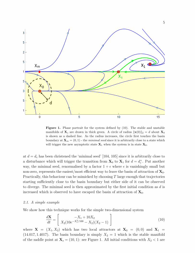
Figure 1. Phase portrait for the system defined by (10). The stable and unstable

manifolds of Xs are drawn in thick green. A circle of radius ‖x(0)‖2 = d about X0

is shown as a dashed line. As the radius increases, the circle first touches the basin

boundary at Xm = (0, 1) - the minimal seed since it is arbitrarily close to a state which

will trigger the new asymptotic state X1 when the system is in state X0.

at d = dc has been christened the ‘minimal seed’ [104, 105] since it is arbitrarily close to

a disturbance which will trigger the transition from X0 to X1 for d = d+c . Put another

way, the minimal seed, renormalised by a factor 1 + ε where ε is vanishingly small but

non-zero, represents the easiest/most efficient way to leave the basin of attraction of X0.

Practically, this behaviour can be mimicked by choosing T large enough that trajectories

starting sufficiently close to the basin boundary but either side of it can be observed

to diverge. The minimal seed is then approximated by the first initial condition as d is

increased which is observed to have escaped the basin of attraction of X0.

2.1. A simple example

We show how this technique works for the simple two-dimensional system

dX

dt=

[−X1 + 10X2

X2(10e−X21/100 −X2)(X2 − 1)

](10)

where X = (X1, X2) which has two local attractors at X0 = (0, 0) and X1 =

(14.017, 1.4017). The basin boundary is simply X2 = 1 which is the stable manifold

of the saddle point at Xs = (10, 1): see Figure 1. All initial conditions with X2 < 1 are

6

0 0.5 1 1.5 20

0.005

0.01

0.015

0.02

0.025

0.03

0.035

0.04

0.045

0 0.5 1 1.5 20

0.05

0.1

0.15

0.2

0.25

0 0.5 1 1.5 20

5

10

15

0 0.5 1 1.5 20

50

100

150

200

250

Figure 2. Top row: Gain G := ‖x(t)‖22/d2 versus θ for T = 2 and d = 10−4 (top left)

or 0.9 (top right). Bottom row: ‖x(T )‖22 versus θ for T = 2 and d = 0.9999 (bottom

left) or 1.0001 (solid line, bottom right) and 1.2 (dashed line, bottom right). Notice

the sudden jump in ‖x(T )‖22 when d increases from 0.9999 to 1.0001 signalling that

the basin boundary of X0 has been crossed ( ‖x(T )‖22 is simply 100(1− e−T )2 + 1 for

d = dc ).

attracted to X0, those with X2 > 1 to X1, and those with X2 = 1 to Xs. Focussing

on the ‘unexcited’ state X0, x := X − X0 and using the Euclidean norm again for

simplicity, it is clear that drawing a circle in the (x1, x2) plane centred on the origin and

of increasing radius d, the basin boundary for X0 will be first touched at d = dc = 1

where (x1, x2) = (0, 1): this is the minimal seed for this system. As d increases beyond

dc, the basin boundary is increasingly punctured so that ever more initial conditions are

outside of the basin of attraction of X0.

This observation can be deduced by iteratively solving the optimisation problem

described above through integrating (10) forwards (since here x = X as X0 = 0) to find

x(t) and the dual dynamical equation

dν

dt=

[ν1 + 1

5x1ν2(x

22−x2)e−x

21/100

−10ν1+ ν2(3x22−2x2)−10ν2(2x2−1)e−x

21/100

](11)

7

0.95 0.96 0.97 0.98 0.99 1 1.01 1.02 1.03 1.04 1.050

50

100

150

200

250 c

max

‖x(T

)‖2 2

d

d

0.5

0.75

1

5

Figure 3. As T (labelled on each curve) increases, the signature of the transition

at dc becomes increasingly clear. Note only for T → ∞ is the final plateau

‖x(T )‖22 = ‖X1 −X0‖22 ≈ 198.5 as x(t) ‘overshoots’: see Figure 1.

for ν(t) backwards (note that this backwards-in-time integration requires knowledge

of x(t) across [0, T ]). Figure 2 shows how ‖x(T )‖22 varies over all permitted initial

conditions parameterised by the angle θ ∈ [0, 2) where

x(0) = ( d cos πθ, d sin πθ ) (12)

for selected values of d and T = 2 (note the gain G := ‖x(T )‖22/d2 is plotted for the top

row of subplots since d has such different values). The small value d = 10−4 is used to

reproduce the linear result obtainable via standard matrix manipulations (see Appendix

A) which possesses the x(0) → −x(0) (θ → θ ± 1) symmetry. As d is increased, this

symmetry is quickly destroyed as nonlinearity becomes important to indicate a unique

optimal value of θ approaching 0.5 as d → dc. Once d reaches dc, ‖x(T )‖22 jumps in

value as the system explores the basin boundary and then (for d > dc) the basin of

attraction of X1. Three key points highlighted by this simple example are as follows.

(i) The importance of T in determining dc to a required accuracy. Figure 3 shows that

dc is increasingly well identified as the value of T increases or if T is too small, the

jump in ‖x(T )‖2 at d = dc is smeared out and so difficult to locate. On a practical

level, T should not be chosen too large as the optimisation procedure becomes

increasingly sensitive to changes in the starting state.

(ii) The minimal seed is not related to the linear optimal. For ‘large’ T (≥ 2), the

minimal seed has θ∗ = 0.5 (90o) whereas the linear optimal (d→ 0) has θ∗ ≈ 0.2667

(48.0o). This is not surprising since phase space immediately around X0 is generally

8

unrelated to the structure of the basin boundary a finite distance away. (The one

caveat to this is if the nonlinear terms had been chosen to be energy-preserving -

e.g. the model system studied in [30]. In this case, the dynamics are so tightly

constrained in 2 dimensions that the minimal seed has to be the same as the linear

optimal: see Appendix B for further discussion.)

(iii) The Euclidean norm works well as there is little growth for trajectories with x2 < 1,

whereas trajectories in x2 > 1 overshoot X1. If this were not the case, the functional

to optimise - the objective functional - could be redesigned to signal the arrival in a

new basin. Here for example, the value of x2(T ) would be more appropriate with the

Euclidean norm still used to constrain the competitor set of initial perturbations,

i.e. the measure used as the objective functional and the norm constraining the

initial condition do not need to be the same.

3. The Transition to Turbulence problem in Fluid Mechanics

We now move the discussion to fluid mechanics and a system described by a set of

PDEs. The breakdown of laminar shear flows has been a central problem in fluid

mechanics since the inception of the subject and fascinated many generations of scientists

(e.g. Rayleigh [110], Kelvin [127], Reynolds [114, 115], Orr [99], Sommerfeld [124],

Noether [97], Taylor [125], Heisenberg [58], Landau [78], Hopf [61] and see the textbooks

[17, 33, 32, 117]). Beyond a certain value of the driving rate (measured by a non-

dimensional grouping called the Reynolds number Re and generated by either imposed

boundary motion, flow rate or pressure gradient), unidirectional shear flows (e.g. flow

through a straight pipe) typically exhibit bi stability where a linearly-stable simple

laminar state coexists with a spatially- and temporally-complicated turbulent state.

The so-called ‘transition’ problem consists in understanding the physical processes by

which ambient noise (present in any real flow) can trigger the observed transition of the

flow from the laminar to the turbulent state. The fact that the laminar state is linearly

stable means that the transition process is inherently nonlinear and even now still largely

unexplained. The transition problem is not only a fascinating mathematical exercise in

PDE theory, but the answers are crucial for informing attempts to inhibit (e.g. in the

aircraft industry) or enhance (e.g. crucial for mixing processes) the phenomenon in

practical applications.

In the last two decades or so, two complementary approaches to the transition

problem have proved popular. The first - variously labelled ‘transient growth’,

‘nonmodal stability theory’ or ‘optimal perturbation theory’ - is a linear theory

explaining how, due to the non-normality of the linearised evolution operator† about the

laminar state, infinitesimal disturbances can experience large but transient magnification

of their energy despite the laminar state being asymptotically stable (all the eigenvalues

indicate exponential decay with time). This idea has a long history starting with Kelvin

† An operator/matrix L is non-normal if it does not commute with its adjoint/transpose L† i.e.

LL† 6= L†L.

9

[127] and Orr [99] but has really only been systematically explored from the late 1980s

onwards: see [12, 43, 57, 15, 130, 111], the reviews [54, 113, 116, 118] and the books

[117, 131]. The theory works well for interpreting finite time behaviour such as the

flow response to noise immediately downstream of a pipe expansion [16] but actually

says nothing about asymptotically long time behaviour. Initially, it was suggested that

the presence of large transient growth could ‘elevate’ infinitesimal disturbances into the

nonlinear regime where they could then become sustained (e.g. [4, 5]). While this

picture, which emphasizes linear effects over nonlinearity, must be generally correct

(as only linear effects can give rise to energy growth), no quantitative predictions of

transition amplitudes can emerge without a fully nonlinear theory [133, 30].

The second approach to the transition problem, on the other hand, is fully nonlinear.

This views the flow as a dynamical system and the flow state as an evolving trajectory

in a phase space populated by various invariant sets (exact solutions) and their stable

and unstable manifolds [38, 73, 39, 53, 29, 72]. From this perspective, ‘transition’ occurs

when noise or a disturbance simply nudges the flow out of the basin of attraction of the

laminar state. Making this observation more predictive has, however, been extremely

hard due to the difficulty of mapping out the basin boundary. Some progress has been

made shadowing the basin boundary (or the more general concept of an ‘edge’, which

includes transient turbulence) forward in time using an ‘edge tracking’ technique. This

finds ‘edge states’ which are saddles in the full phase space but attractors on the basin

boundary [63, 123, 119] (e.g. Xs in Figure 1). However, these are invariably more distant

(energetically) from the laminar state [105] than other parts of the basin boundary and

therefore less obviously relevant for choosing an initial transition-triggering disturbance.

What is really needed is a technique to track the basin boundary backwards in time to

reach regions where it is close to the laminar state.

The gap between these two approaches is therefore one of perspective: the optimal

perturbation theory explains how infinitesimal disturbances can grow temporarily within

the basin boundary whereas the dynamical systems approach focusses on what exists

beyond the basin boundary. The new optimisation technique discussed in this article

naturally bridges this gap by being able to examine how the optimal perturbation

deviates from the linear optimal as the amplitude of the starting perturbation is

increased until the basin boundary is reached. The original thinking behind the studies

[104, 105], however, was a little different being focussed on tracing the basin boundary

or edge ‘backwards’ in time by posing an optimisation problem. If the edge state found

by edge tracking is unique then for all starting states on the basin boundary, the initial

state which subsequently experiences the largest energy growth over asymptotically large

times (so that all trajectories reach the edge state) will be the minimal seed [105]. While

this optimisation problem itself is intractable because the basin boundary is unknown, it

does suggest the tractable problem of finding the largest energy growth over all starting

states of a given initial energy E0. At precisely E0 = Ec, where the basin boundary or

edge touches the energy hypersurface at one velocity state, this optimization problem

considers the growth of this state (the minimal seed) against the energy growth of all the

10

other initial conditions below the edge. Given that these latter initial conditions lead to

flows that grow initially but ultimately relax back to the basic state, the minimal seed

will remain the optimal initial condition for the revised optimisation problem for large

enough T [105]. The simple choice of the kinetic energy of the disturbance as both the

objective functional and the constraining norm meant that the vanishing energy limit

E0 → 0 lead back to the familiar linear optimal perturbation calculation. It is now clear

other choices could have been made for the objective functional providing it takes on

heightened values for the turbulent state (e.g energy dissipation [86, 37] and [47, 48] for

work considering different norms).

Before giving an example of the optimisation technique at work in fluid mechanics,

we note that there have been many previous efforts to build upon (linear) optimal

perturbation theory to design better ways to trigger transition. For example (since

space prevents an exhaustive listing), by considering secondary transient growth on top

of a linear optimal (e.g. [122, 60, 27]), or by probing its finite amplitude stability (e.g.

[28]), or by showing that the linear optimals can become linearly unstable at sufficient

amplitude (e.g. [139, 112]). Finite amplitude initial disturbances have also been designed

from a very small set of physically-motivated ‘basis’ states (e.g. [132, 36]) and optimal

deformations of the base flow found so as to create linear instability [13, 10, 52, 11]. All

this work either focusses on one possible aspect of the transition process or makes some

assumption about disturbances able to trigger transition efficiently. In contrast, no such

assumptions are made in what follows.

3.1. The optimisation technique in pipe flow

We now show the optimisation technique in action for the problem of incompressible

fluid flow through a cylindrical pipe. This is a classical problem in fluid mechanics

studied famously by Reynolds [114, 115] during which he first wrote down the non-

dimensional grouping Re now bearing his name. The flow can either be driven by

imposing a constant pressure drop across the pipe or by imposing a constant mass flux

through the pipe (e.g. [96]). We choose the former driving here as the formulation is

slightly simpler (the latter is treated in [104, 105]): the two cases are equivalent for

L → ∞ and localised disturbances. The set up is an incompressible fluid of constant

density ρ and kinematic viscosity ν flowing in a circular pipe of radius s0 under the

action of a constant pressure drop imposed across the pipe of

∆p∗ = −4ρνW

s0L (13)

(where the pipe is L radii long) and the (basic) Hagen-Poiseuille solution to the Navier-

Stokes equations is

u∗lam := W(

1− s∗2

s20

)z∗, p∗lam := −4ρνW

s20z∗ (14)

in the usual cylindrical coordinates (s∗, φ, z∗) aligned with the pipe axis. Non-

dimensionalizing the system using the Hagen-Poiseuille centreline speed W (e.g. ulam :=

11

u∗lam/W ) and the pipe radius s0 (so s := s∗/s0) gives the Navier-Stokes equations

∂utot

∂t+ utot ·∇utot + ∇ptot =

1

Re∇2utot (15)

where Re := s0W/ν is the Reynolds number and ptot := p + plam (plam := −4z/Re)

is the total pressure with its deviation, p, from the laminar pressure field periodic

across the length of the pipe to maintain the constant pressure drop: i.e. p(s, φ, z, t) =

p(s, φ, z + L, t). The velocity boundary conditions are

utot(1, φ, z, t) = 0 & utot(s, φ, z, t) = utot(s, φ, z + L, t), (16)

the first being no-slip on the pipe wall at s = 1 and the second periodicity across the pipe

length. We consider the energy growth (our ‘distance’ measure) of a finite-amplitude

disturbance

u := utot − ulam (17)

to the laminar profile ulam = (1− s2)z by defining the Lagrangian

L = L(u, p, λ,ν, π;T,E0) :=

⟨1

2|u(x, T )|2

⟩+ λ

{⟨1

2|u(x, 0)|2

⟩− E0

}+

∫ T

0

⟨ν(x, t) ·

{∂u

∂t+ (ulam ·∇)u + (u ·∇)ulam + (u ·∇)u

+∇p− 1

Re∇2u

}⟩dt+

∫ T

0

〈π(x, t)∇ · u〉 dt. (18)

where

〈. . .〉 =

∫ L

0

∫ 2π

0

∫ 1

0

. . . sds dφ dz (19)

and λ, ν and π are Lagrangian multipliers imposing the constraints that the initial

energy is fixed, that the Navier-Stokes equation holds over t ∈ [0, T ] and the flow is

incompressible. Their corresponding Euler-Lagrange equations are respectively:⟨1

2|u(x, 0)|2

⟩= E0 (20)

∂u

∂t+ (ulam ·∇)u + (u ·∇)ulam + (u ·∇)u + ∇p− 1

Re∇2u = 0, (21)

∇ · u = 0. (22)

The key additions to the well-known linear calculation acknowledging the fact that the

disturbance is of finite amplitude are shown in red. The linearised problem is recovered

in the limit of E0 → 0 whereupon the nonlinear term u ·∇u becomes vanishingly small

relative to the other (linear) terms. On dropping this nonlinear term, the amplitude of

the disturbance is then arbitrary for the purposes of the optimisation calculation and it

is convenient to reset E0 from vanishingly small to 1. In this case the maximum of L is

then precisely the maximum gain in energy over the period [0, T ].

12

The Euler-Lagrange equation for the pressure p is

0 =

∫ T

0

⟨δLδpδp

⟩dt =

∫ T

0

〈(ν ·∇)δp〉 dt

=

∫ T

0

〈∇ · (νδp)〉 dt−∫ T

0

〈δp(∇ · ν)〉 dt. (23)

which vanishes if ν satisfies natural boundary conditions (which turn out here to be the

same as those for u) and

∇ · ν = 0 (24)

(note δp is periodic across the pipe to ensure the pressure drop across the pipe is

constant). The variation in L due to u (with δu satisfying (16) ) is

δL =

∫ T

0

⟨δLδu· δu

⟩= 〈u(x, T ) · δu(x, T )〉+ λ 〈u(x, 0) · δu(x, 0)〉

+

∫ T

0

⟨ν ·{∂δu

∂t+ (ulam ·∇)δu + (δu ·∇)ulam

+u.∇δu + δu ·∇u− 1

Re∇2δu

}⟩dt+

∫ T

0

〈π∇ · δu〉 dt. (25)

The first term in the second line of the above equation can be reexpressed as∫ T

0

⟨ν · ∂δu

∂t

⟩dt =

∫ T

0

⟨∂

∂t(δu · ν)

⟩dt−

∫ T

0

⟨δu · ∂ν

∂t

⟩dt

= 〈δu(x, T ) · ν(x, T )− δu(x, 0) · ν(x, 0)〉 −∫ T

0

⟨δu · ∂ν

∂t

⟩dt. (26)

Similarly, the second term is

〈ν · {(ulam ·∇)δu}〉 = 〈∇ · ((ν · δu)ulam)− δu · {(ulam ·∇)ν}〉= −〈δu · {(ulam ·∇)ν}〉 . (27)

The third term is

〈ν · {(δu ·∇)ulam}〉 =⟨δu ·

{ν · (∇ulam)T

}⟩(= 〈δui νj ∂iulam,j〉). (28)

The fourth and fifth terms are

〈ν · (δu ·∇u + u ·∇δu)〉 =⟨δu ·

([∇u]T · ν − u ·∇ν

)⟩, (29)

the sixth term is⟨ν ·(− 1

Re∇2δu

)⟩= −

⟨1

Reδu · ∇2ν

⟩, (30)

and finally the last term is

〈π∇ · δu〉 = 〈∇ · πδu〉 − 〈δu ·∇π〉= −〈δu · ∇π〉 , (31)

13

where π has to be periodic as 〈δu · z〉 6= 0 (a change in the mass flux is permitted for

constant pressure-drop driven flow) for the surface term to be zero. Combining all these

gives ∫ T

0

⟨δLδu· δu

⟩= 〈δu(x, T ) · {u(x, T ) + ν(x, T )}〉

+ 〈δu(x, 0) · {λu(x, 0)− ν(x, 0)}〉

+

∫ T

0

⟨δu ·

{−∂ν∂t− ([ulam + u] ·∇)ν + ν · (∇[ulam + u])T

−∇π − 1

Re∇2ν

}⟩dt. (32)

For this to vanish for all allowed δu(x, T ), δu(x, 0) and δu(x, t) with t ∈ (0, T ) means

δLδu(x, T )

= 0 ⇒ u(x, T ) + ν(x, T ) = 0, (33)

δLδu(x, 0)

= 0 ⇒ λu(x, 0)− ν(x, 0) = 0, (34)

δLδu

= 0 ⇒ ∂ν

∂t+ (ulam + u) ·∇ν − ν · (∇[ulam + u])T + ∇π +

1

Re∇2ν = 0. (35)

This last equation is the dual (or adjoint) Navier-Stokes equation for evolving ν

backwards in time because of the negative diffusion term. This dual equation has the

same means of driving - constant pressure drop - as the physical problem, a situation

also true for the constant mass-flux situation [104, 105].

The approach for tackling this optimization problem - ‘nonlinear adjoint looping’

- is iterative as in the linear situation [81, 2, 25, 82, 55] (see also the review [83]), the

nonlinear calculation of [141, 142] using the (parabolic) boundary layer equations and

more generally [56]. It is essentially as outlined in §2.

Step 0. Choose an initial condition u(0)(x, 0) such that⟨1

2|u(0)(x, 0)|2

⟩= E0. (36)

The (better) next iterate u(n+1)(x, 0) is then constructed from u(n)(x, 0) as follows:

Step 1. Time integrate the Navier-Stokes equation (21) forward with incompressibility

∇ · u = 0 and using the boundary conditions (16) from t = 0 to t = T with the

initial condition u(n)(x, 0) to find u(n)(x, T ).

Step 2. Calculate ν(n)(x, T ) using (33) which is then used as the initial condition for

the dual Navier-Stokes equation (35).

Step 3. Backwards time integrate the dual Navier-Stokes equation (35) with

incompressibility (24) and boundary conditions (16) from t = T to t = 0 with

the ‘initial’ condition ν(n)(x, T ) to find ν(n)(x, 0).

14

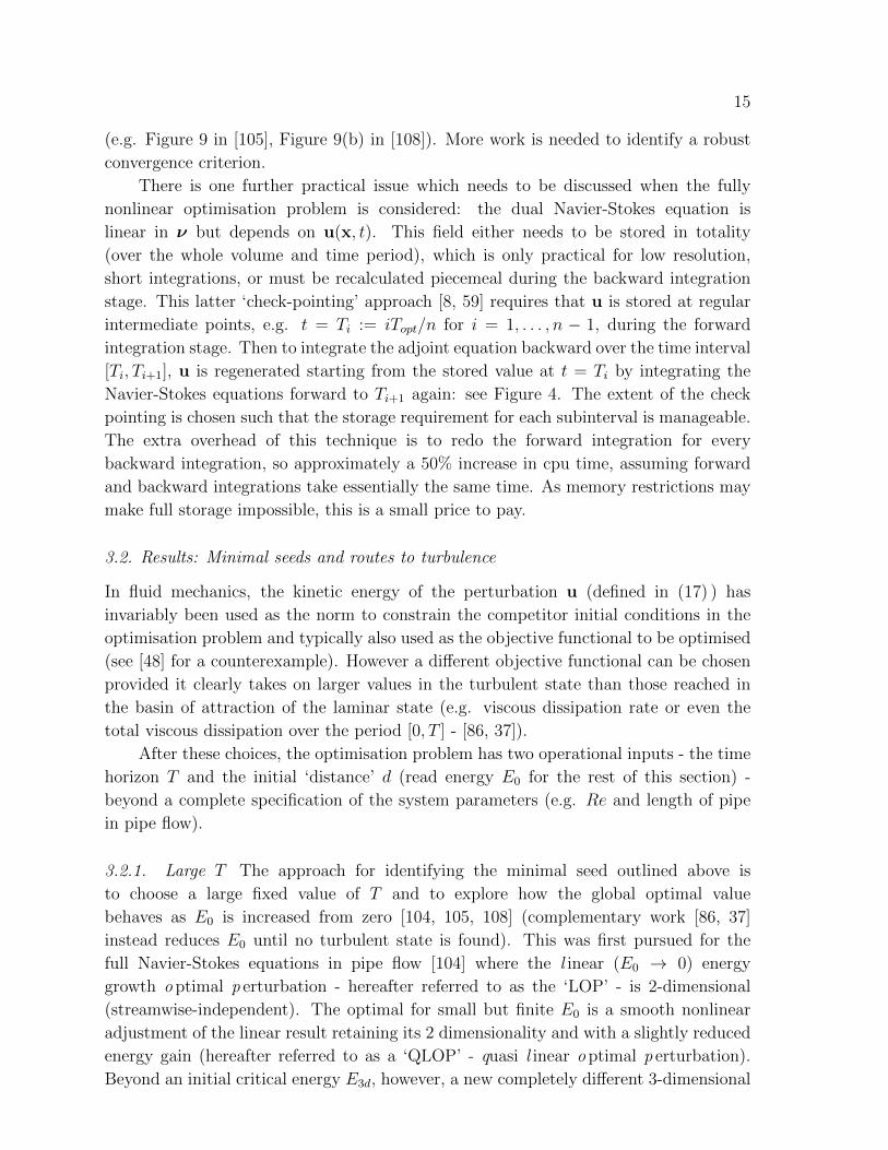
t=0 t=T

u(x,t)

ν(x,t)

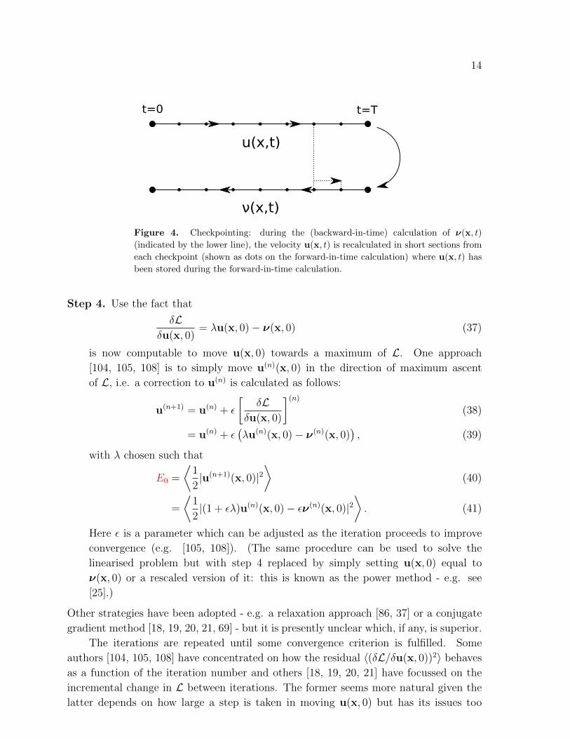
Figure 4. Checkpointing: during the (backward-in-time) calculation of ν(x, t)

(indicated by the lower line), the velocity u(x, t) is recalculated in short sections from

each checkpoint (shown as dots on the forward-in-time calculation) where u(x, t) has

been stored during the forward-in-time calculation.

Step 4. Use the fact that

δLδu(x, 0)

= λu(x, 0)− ν(x, 0) (37)

is now computable to move u(x, 0) towards a maximum of L. One approach

[104, 105, 108] is to simply move u(n)(x, 0) in the direction of maximum ascent

of L, i.e. a correction to u(n) is calculated as follows:

u(n+1) = u(n) + ε

[δL

δu(x, 0)

](n)(38)

= u(n) + ε(λu(n)(x, 0)− ν(n)(x, 0)

), (39)

with λ chosen such that

E0 =

⟨1

2|u(n+1)(x, 0)|2

⟩(40)

=

⟨1

2|(1 + ελ)u(n)(x, 0)− εν(n)(x, 0)|2

⟩. (41)

Here ε is a parameter which can be adjusted as the iteration proceeds to improve

convergence (e.g. [105, 108]). (The same procedure can be used to solve the

linearised problem but with step 4 replaced by simply setting u(x, 0) equal to

ν(x, 0) or a rescaled version of it: this is known as the power method - e.g. see

[25].)

Other strategies have been adopted - e.g. a relaxation approach [86, 37] or a conjugate

gradient method [18, 19, 20, 21, 69] - but it is presently unclear which, if any, is superior.

The iterations are repeated until some convergence criterion is fulfilled. Some

authors [104, 105, 108] have concentrated on how the residual 〈(δL/δu(x, 0))2〉 behaves

as a function of the iteration number and others [18, 19, 20, 21] have focussed on the

incremental change in L between iterations. The former seems more natural given the

latter depends on how large a step is taken in moving u(x, 0) but has its issues too

15

(e.g. Figure 9 in [105], Figure 9(b) in [108]). More work is needed to identify a robust

convergence criterion.

There is one further practical issue which needs to be discussed when the fully

nonlinear optimisation problem is considered: the dual Navier-Stokes equation is

linear in ν but depends on u(x, t). This field either needs to be stored in totality

(over the whole volume and time period), which is only practical for low resolution,

short integrations, or must be recalculated piecemeal during the backward integration

stage. This latter ‘check-pointing’ approach [8, 59] requires that u is stored at regular

intermediate points, e.g. t = Ti := iTopt/n for i = 1, . . . , n − 1, during the forward

integration stage. Then to integrate the adjoint equation backward over the time interval

[Ti, Ti+1], u is regenerated starting from the stored value at t = Ti by integrating the

Navier-Stokes equations forward to Ti+1 again: see Figure 4. The extent of the check

pointing is chosen such that the storage requirement for each subinterval is manageable.

The extra overhead of this technique is to redo the forward integration for every

backward integration, so approximately a 50% increase in cpu time, assuming forward

and backward integrations take essentially the same time. As memory restrictions may

make full storage impossible, this is a small price to pay.

3.2. Results: Minimal seeds and routes to turbulence

In fluid mechanics, the kinetic energy of the perturbation u (defined in (17) ) has

invariably been used as the norm to constrain the competitor initial conditions in the

optimisation problem and typically also used as the objective functional to be optimised

(see [48] for a counterexample). However a different objective functional can be chosen

provided it clearly takes on larger values in the turbulent state than those reached in

the basin of attraction of the laminar state (e.g. viscous dissipation rate or even the

total viscous dissipation over the period [0, T ] - [86, 37]).

After these choices, the optimisation problem has two operational inputs - the time

horizon T and the initial ‘distance’ d (read energy E0 for the rest of this section) -

beyond a complete specification of the system parameters (e.g. Re and length of pipe

in pipe flow).

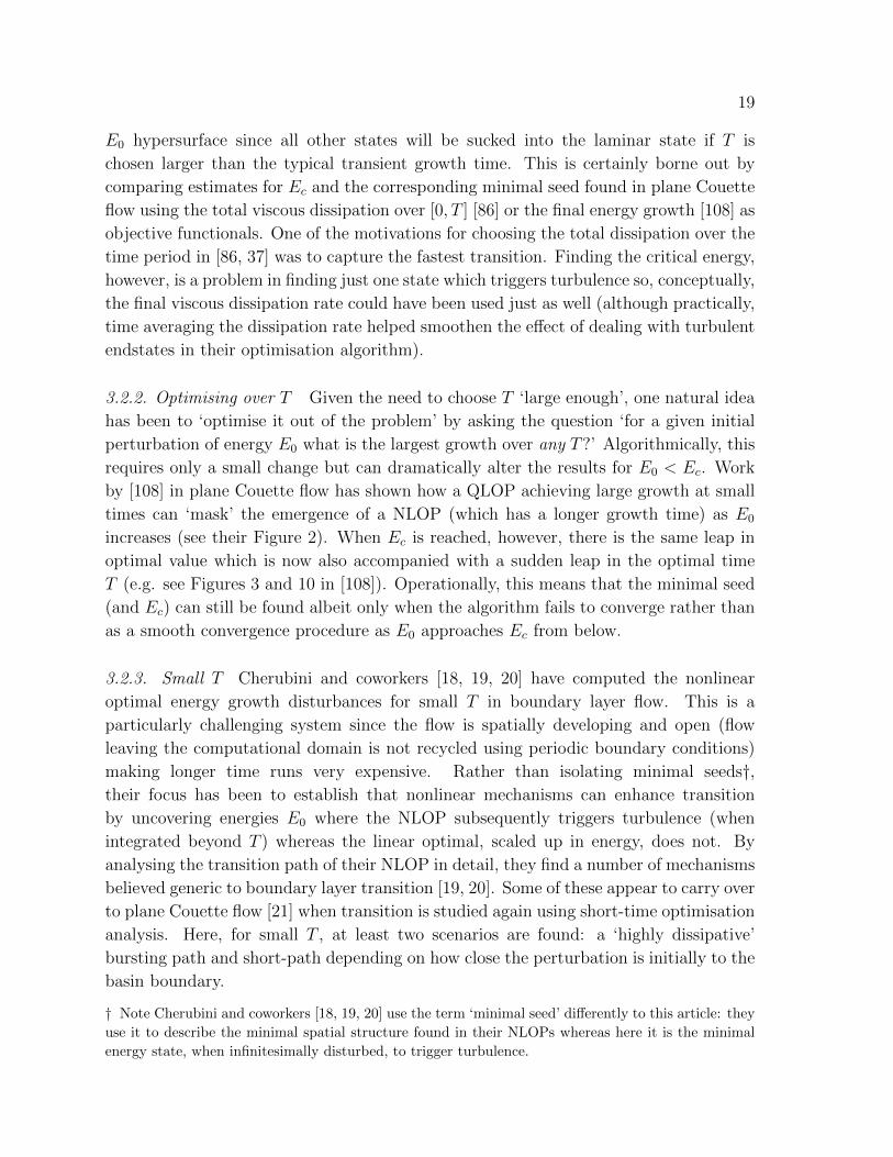
3.2.1. Large T The approach for identifying the minimal seed outlined above is

to choose a large fixed value of T and to explore how the global optimal value

behaves as E0 is increased from zero [104, 105, 108] (complementary work [86, 37]

instead reduces E0 until no turbulent state is found). This was first pursued for the

full Navier-Stokes equations in pipe flow [104] where the l inear (E0 → 0) energy

growth o ptimal p erturbation - hereafter referred to as the ‘LOP’ - is 2-dimensional

(streamwise-independent). The optimal for small but finite E0 is a smooth nonlinear

adjustment of the linear result retaining its 2 dimensionality and with a slightly reduced

energy gain (hereafter referred to as a ‘QLOP’ - quasi l inear o ptimal p erturbation).

Beyond an initial critical energy E3d, however, a new completely different 3-dimensional

16

0 5 10 15 20 250

50

100

150

200

250

300

350

400E

(t)/

E0

time (D/U)

Figure 5. Pipe flow: the evolution of the linear and nonlinear energy growth optimals

at Re = 1750 in a pipe of length π radii and constant flux [104]. The blue dashed

line corresponds to the linear optimal for E0 → 0 whereas the red solid line is the

nonlinear optimal for ≈ 1.5E3d both calculated using (a short) T equal to the linear

growth optimal time shown as a vertical black dotted line (the nonlinear optimal

actually produces even more growth at a slightly earlier time).

perturbation was found as the global optimal and christened the ‘NLOP’ (nonl inear

o ptimal p erturbation) [104]: see Figure 5. This NLOP reflects a clear strategy by the

fluid to spatially localise the starting perturbation so that its peak amplitude is larger

but only over a limited volume to cheat the global energy constraint. The original pipe

geometry used in [104] was very short so the NLOP is only localised in the radial and

azimuthal directions (see Figure 2(a) in [104]). Subsequent computations in much longer

pipe geometries have confirmed that the NLOP fully localises by also localising in the

axial (streamwise) direction too [105, 106]: see Figure 7. Physically, the NLOP evolves

by initially ‘unpacking’ (delocalising) under the influence of the background shear flow

and taking advantage of 3 distinct well-known linear mechanisms for transient growth:

the Orr mechanism which occurs quickly, oblique wave growth which operates over an

intermediate timescale, and lift-up which occurs over a slow timescale (see [105, 37] and

references therein). These mechanisms are unrelated in the linear problem i.e. initial

conditions exploiting each are distinct from each other so that the mechanisms do not

17

0 50 100 150 2000

2000

4000

6000

8000

10000

12000

14000

16000E

(t)/

E0

time (in D/U)

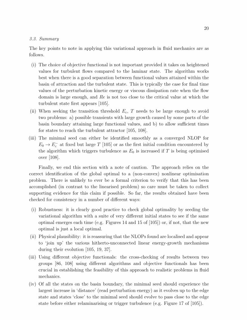
Figure 6. Pipe flow: the evolution of the energy growth optimals at Re = 2400 in

a constant-flux pipe of length 10 radii using a ‘large’ time T = 75D/U indicated by

a vertical black dotted line (see section 5 of [105]). The thin blue lines correspond to

the NLOPs for two E0s just below Ec (within 1%) with turbulence not triggered. The

thick red solid line is for E0 just above Ec (again within 1%) and turbulence is now

clearly triggered (see Figure 7 for snapshots of this evolution).

combine. However they can communicate with the addition of nonlinearity which allows

each mechanism to ‘pump prime’ the next generating a much higher overall growth

[105, 37]. Figure 5 shows a period of growth in the NLOP curve (the oblique wave

growth stage) which terminates at t ≈ 2.5 before further growth (lift up) occurs until

t ≈ 16 (the Orr mechanism occurs over a much faster timescale - O(0.1) see Figure 1 of

[105] - and is therefore hidden in this plot). Appendix B discusses a very simple model

to illustrate this phenomenon (compare Figures 5 and 9).

As E0 is increased further, this NLOP remains the global optimal until another

critical energy Efail is reached beyond which the optimisation procedure fails to

converge. Pringle et al. [105] interpret (their conjecture 1) that this corresponds to

the first energy at which an initial condition can reach the turbulent state since then

the extreme sensitivity of the final-state energy at T to changes in the initial condition,

due to exponential divergence of adjacent states will effectively mean non-smoothness

and prevent convergence. That the turbulent state has been reached at Efail is easily

18

Figure 7. Pipe flow: snapshots showing the evolution (time running downwards and

fluid flow left to right) of a turbulence-triggering perturbation which approximates

the minimal seed in a 10 radii long pipe at Re = 2400 (constant flux) [105] (the

corresponding evolution of the total energy is shown as the red thick line in Figure

6). The isocontours in each plot correspond to 50% of the maximum (light/yellow)

and 50% of the minimum (dark/red) of the streamwise perturbation velocity in the

pipe at t = 0 (top: essentially the minimal seed), t = 5 (second down), t = 20 (third

down) and t = 75D/U (bottom: the target time). The perturbation energy is initially

localised but quickly spreads out to generate streamwise streaks (by t ≈ 10) which

then break up to generate turbulence.

confirmed by examining the endstates u(x, T ) reached as part of the iteration algorithm

so that Efail is at least an upper bound on the true critical energy Ec, which is the

lowest energy at which turbulence can be triggered. Arguing that in fact Efail = Ecrequires a belief or hope that the search algorithm will find any state on the (initial)

energy hypersurface which can reach the turbulent state if it exists. This is never likely

to be proved but can at least be made plausible by rerunning the algorithm with a

variety of initial starting states (e.g. see Figure 14 in [105]).

Pringle et al. [105] also noticed (their conjecture 2) that the NLOP converged to

the minimal seed as E0 → E−c for their choice of the energy functional. It now seems

clear that there is nothing special about using the perturbation energy as an objective

functional merely that it is one of a class of functionals which take on heightened values

for turbulent flows. Providing such a functional is chosen, the best way to maximise

it should be to get as close to the basin boundary as possible while remaining on the

19

E0 hypersurface since all other states will be sucked into the laminar state if T is

chosen larger than the typical transient growth time. This is certainly borne out by

comparing estimates for Ec and the corresponding minimal seed found in plane Couette

flow using the total viscous dissipation over [0, T ] [86] or the final energy growth [108] as

objective functionals. One of the motivations for choosing the total dissipation over the

time period in [86, 37] was to capture the fastest transition. Finding the critical energy,

however, is a problem in finding just one state which triggers turbulence so, conceptually,

the final viscous dissipation rate could have been used just as well (although practically,

time averaging the dissipation rate helped smoothen the effect of dealing with turbulent

endstates in their optimisation algorithm).

3.2.2. Optimising over T Given the need to choose T ‘large enough’, one natural idea

has been to ‘optimise it out of the problem’ by asking the question ‘for a given initial

perturbation of energy E0 what is the largest growth over any T?’ Algorithmically, this

requires only a small change but can dramatically alter the results for E0 < Ec. Work

by [108] in plane Couette flow has shown how a QLOP achieving large growth at small

times can ‘mask’ the emergence of a NLOP (which has a longer growth time) as E0

increases (see their Figure 2). When Ec is reached, however, there is the same leap in

optimal value which is now also accompanied with a sudden leap in the optimal time

T (e.g. see Figures 3 and 10 in [108]). Operationally, this means that the minimal seed

(and Ec) can still be found albeit only when the algorithm fails to converge rather than

as a smooth convergence procedure as E0 approaches Ec from below.

3.2.3. Small T Cherubini and coworkers [18, 19, 20] have computed the nonlinear

optimal energy growth disturbances for small T in boundary layer flow. This is a

particularly challenging system since the flow is spatially developing and open (flow

leaving the computational domain is not recycled using periodic boundary conditions)

making longer time runs very expensive. Rather than isolating minimal seeds†,their focus has been to establish that nonlinear mechanisms can enhance transition

by uncovering energies E0 where the NLOP subsequently triggers turbulence (when

integrated beyond T ) whereas the linear optimal, scaled up in energy, does not. By

analysing the transition path of their NLOP in detail, they find a number of mechanisms

believed generic to boundary layer transition [19, 20]. Some of these appear to carry over

to plane Couette flow [21] when transition is studied again using short-time optimisation

analysis. Here, for small T , at least two scenarios are found: a ‘highly dissipative’

bursting path and short-path depending on how close the perturbation is initially to the

basin boundary.

† Note Cherubini and coworkers [18, 19, 20] use the term ‘minimal seed’ differently to this article: they

use it to describe the minimal spatial structure found in their NLOPs whereas here it is the minimal

energy state, when infinitesimally disturbed, to trigger turbulence.

20

3.3. Summary

The key points to note in applying this variational approach in fluid mechanics are as

follows.

(i) The choice of objective functional is not important provided it takes on heightened

values for turbulent flows compared to the laminar state. The algorithm works

best when there is a good separation between functional values attained within the

basin of attraction and the turbulent state. This is typically the case for final time

values of the perturbation kinetic energy or viscous dissipation rate when the flow

domain is large enough, and Re is not too close to the critical value at which the

turbulent state first appears [105].

(ii) When seeking the transition threshold Ec, T needs to be large enough to avoid

two problems: a) possible transients with large growth caused by some parts of the

basin boundary attaining large functional values, and b) to allow sufficient times

for states to reach the turbulent attractor [105, 108].

(iii) The minimal seed can either be identified smoothly as a converged NLOP for

E0 → E−c at fixed but large T [105] or as the first initial condition encountered by

the algorithm which triggers turbulence as E0 is increased if T is being optimised

over [108].

Finally, we end this section with a note of caution. The approach relies on the

correct identification of the global optimal to a (non-convex) nonlinear optimisation

problem. There is unlikely to ever be a formal criterion to verify that this has been

accomplished (in contrast to the linearised problem) so care must be taken to collect

supporting evidence for this claim if possible. So far, the results obtained have been

checked for consistency in a number of different ways:

(i) Robustness: it is clearly good practice to check global optimality by seeding the

variational algorithm with a suite of very different initial states to see if the same

optimal emerges each time (e.g. Figures 14 and 15 of [105]) or, if not, that the new

optimal is just a local optimal.

(ii) Physical plausibility: it is reassuring that the NLOPs found are localised and appear

to ‘join up’ the various hitherto-unconnected linear energy-growth mechanisms

during their evolution [105, 19, 37].

(iii) Using different objective functionals: the cross-checking of results between two

groups [86, 108] using different algorithms and objective functionals has been

crucial in establishing the feasibility of this approach to realistic problems in fluid

mechanics.

(iv) Of all the states on the basin boundary, the minimal seed should experience the

largest increase in ‘distance’ (read perturbation energy) as it evolves up to the edge

state and states ‘close’ to the minimal seed should evolve to pass close to the edge

state before either relaminarising or trigger turbulence (e.g. Figure 17 of [105]).

21

4. Applications

4.1. Climate modelling and Weather Forecasting

In climate modelling and weather forecasting, the sensitivity of predictive models to

uncertainty in their initial conditions (the current best guess of the model’s state) is

of central importance. Lorenz [80] was the first to introduce the concept of singular

vectors as a way to analyse how this uncertainty (presumed small) may grow with time.

However, it wasn’t until the late 1980s when the idea really took hold following the work

of Farrell [44, 45] in atmospherics and the accompanying realisation in general shear

flows of the phenomenon of (linear) transient growth or (linear) ‘optimal perturbations’

[12, 43, 57, 15, 130, 111]. This quickly led to the implementation of singular vectors to

generate ensemble forecasts (e.g. at the European Centre for Medium-Range forecasting

(ECMWF) [100, 14]).

The initial uncertainties, however, needn’t be small and their true behaviour with

time may differ significantly from that given by the evolution operator linearised around

the base solution. As a result, there have been attempts to include some nonlinearity

into the problem by an iterative approach [98, 6] as well as a proposal for a fully nonlinear

approach by Mu and coworkers: [87, 88, 90, 91, 92] and more recently [35, 140, 66]. [88]

in particular introduced the concept of a ‘conditional nonlinear optimal perturbation’

(CNOP), which is exactly the NLOP discussed above, to study the predictability of

a very simple coupled atmosphere-ocean model. The approach has subsequently been

applied to other weather and climate events (e.g. El Nino events [138, 95, 34], ‘blocking’

onset [65, 91, 94] and the Kuroshio large meander [134, 135]) and extended to treat

uncertainties in a model’s parameters as well [93]. As mentioned in the Introduction,

the idea to study the transitions between different stable states was also suggested by

Mu and co-workers in the context of ocean modelling where multiple equilibria are

a generic feature of general circulation models. To illustrate this idea, [89] studied

a very simple box model of the thermohaline circulation consisting of 2 ODEs using

CNOPs. Subsequent work has tried to scale up the calculation of CNOPs to realistic

PDE models with [90] computing CNOPs for a 2D quasigeostrophic model with 512

grid points and [126] treating a 2D barotropic double-gyre ocean flow model with 4800

degrees of freedom. The latter study, however, concluded that finding basin boundaries

was just too computationally expensive to attempt. Given the recent successes in the

transition problem, this conclusion probably deserves to be revisited.

Before leaving this section, the work of Toth and Kalnay [128, 129, 71] on the so

called ‘breeding’ method deserves mention. This consists of adding a small arbitrary

perturbation to the full forecasting model, allowing this to evolve and then rescaling it

after a given time to reseed the next forecast period. This procedure, which breeds ‘bred

vectors’, is less optimal in identifying optimal perturbations for a given period (in fact

perturbations which emerge have just grown the fastest rather than will grow the fastest)

but is readily generalised to incorporate the finite-amplitude nature of the uncertainties

since the full forecasting model is used. This method is used to generate ensemble

22

forecasts at the National Centers for Environmental Prediction (NCEP) (formerly the

US National Meteorological Center).

4.2. Thermoacoustics

The idea of using an optimisation approach to locate a basin boundary was also

introduced to the field of thermoacoustics at the same time as in the transition to

turbulence community. [69] treated a simple model of thermoacoustic system - a

horizontal Rijke tube - where the laminar state is a fixed point, the edge state is an

unstable periodic orbit and the ‘turbulent’ state is a stable periodic orbit (respectively

the ‘lower’ and ‘upper’ branches which emerge from a saddle node bifurcation). In

contrast with the strategy outlined above, [69] found the minimal seed by looking for

the minimal energy state to reach the (unique) edge state at intermediate times rather

than the minimal energy state that reaches the stable periodic orbit at long times.

However, the result is the same and was confirmed in [70] using the latter strategy.

As in the transition problem (with now the nonlinear terms not energy-preserving), the

minimal seed is found to be completely different from the linear optimal. The Rijke tube

system is sufficiently simple (a couple of time-dependent 1-space dimension PDEs) to

perform an exhaustive survey of transient growth possibilities over amplitude and event

horizon T [70] as well as including noise [136]. It is also realistic enough to achieve some

correspondence with experiments [64].

4.3. Control

Work in controlling fluid flows has long flirted with fully nonlinear methods (e.g.

[67, 68, 56, 9, 23, 103]) but they remain currently very expensive and probably still

impractical [75]. The recent success in identifying NLOPs and minimal seeds, however,

has lead to some new activity in this direction. [101] has recently used the adjoint-based

optimisation procedure discussed here for the full Navier-Stokes equations to control the

2D boundary layer dynamics over a bump by blowing and sucking appropriately through

the boundaries. An extension to 3D has been carried out in [22] where initial conditions

corresponding to the LOP and NLOP have been treated. This work is still some way

short of practical application because it relies on knowing the full state of the system at

each time and costly optimisation computations which can’t be done in real time but it

is at least starting to identify the most promising physical mechanisms for control.

In a slightly different vein, a more nonlinearly stable plane Couette flow has been

designed by imposing spanwise oscillations on the usual streamwise boundary shearing

[109]. This work builds upon the fact that if the critical energy of the minimal seed

can be found then new boundary conditions can be designed to increase this energy

thereby improving the stability of the base state. While the choice of imposing spanwise

oscillations was motivated by a large body of experimental and theoretical work (see

[109] for references), it also meant that the base state was no longer steady but time-

periodic. This has implications for the optimisation procedure which now not only has

23

to search for the optimal initial perturbation but also the exact time (or phase) during

the base flow period when it should be introduced.

4.4. Magnetic field generation & Mixing

[137] treats the kinematic dynamo problem looking for the velocity field of an electrically-

conducting fluid which produces the greatest growth of magnetic field at the end of a

time interval T . The set of competitor fields is constrained either by the total energy

or the L2 norm of their strain rate (or equivalently the viscous dissipation rate) only.

By using the optimisation procedure described here, a lower bound on the magnetic

Reynolds number is identified for a dynamo which is only a 1/5th of that possible

within the well-studied ABC-class of flows [24, 1].

Recently [49] has considered optimal mixing in 2D channel (plane Poiseuille) flow

using a nonlinear optimisation approach. The mixing of a passive scalar, initially

arranged in two layers, is considered in a parameter regime where the flow is linearly

stable. Nonlinear-adjoint looping is used to identify optimal perturbations which lead to

maximal mixing and the classical Taylor dispersion mechanism (where shear enhances

dispersion) is found to emerge naturally from the calculations.

Finally, we close this section by noting that the optimisation procedure discussed

in this article is closely related to the well known data assimilation procedure wherein

a dynamical model of, and incomplete observations about, a real time-evolving system

are used to constrain the initial state of the model such that the ‘best’ solution over

a given time horizon can be sought. This is achieved by minimising an appropriate

cost functional which penalises the deviations of the predicted solution away from

known observations and possible uncertainties in the dynamical model. In contrast,

the optimisation approach discussed here assumes a perfect dynamical model and seeks

to maximise an objective functional over all initial conditions of a certain size in the

absence of constraining observations. Data assimilation is used extensively in many

areas of the geosciences (such as weather forecasting e.g [31, 71], oceanography [7] and

more recently modelling the Earth’s dynamo [50] ).

5. Final summary and future directions

This article has been a pedagogical introduction to an optimisation technique which

offers a new way to probe the basin boundary of a state in a dynamical system.

Although the discussion has concentrated on this well-defined situation for clarity of

exposition, the technique can also usefully be employed for systems with just one global

attractor and at least one long-lived but ultimately-repelling state (sheared fluid flows

with enforced short wavelength dynamics are prime examples of this situation since then

the turbulence seems only transient e.g. [42, 120]). Then the global attractor does not

have a basin boundary but there is instead an ‘edge’ or manifold in phase space which

24

divides initial conditions which immediately converge to the global attractor and those

that first visit one of the repellors. The same game can then be played providing a

functional can be identified which is clearly maximised in the target repellor for a time

long enough for the repellor to be reached yet shorter than the mean lifetime of that

repellor. This is in fact probably the situation in all the fluid flow calculations done so

far (e.g. the turbulence in the 5 diameter long pipe in [105] is actually only transient

at Re = 2400 but the mean lifetime is so large � 100D/U that it mimicks an attractor

on the timescales of the calculations).

The optimisation technique involves maximising a functional which takes on much

larger values in the target state than in the basin of attraction of the starting state

subject to an initial amplitude constraint and other constraints which include that the

governing equations are satisfied - see the summary in §3.3. The iterative approach to

solving this variational problem is not new (e.g [56]) nor is the realisation that there

should be a sudden jump in the optimal value as the initial amplitude increases to

penetrate the basin boundary particularly profound. What is noteworthy, however,

is that the technique appears to work for large degree-of-freedom discretizations of

PDE systems approaching practical application. Typically in such systems, states have

basin boundaries which may be very convoluted in places yet the success reported here

indicates that this needn’t be a serious problem. Whether this is because the minimal

seed for the cases studied so far is away from such areas or that the variational procedure

smoothens over these regions to give an approximate but still good answer remains to

be clarified.

For the particular application studied here - transition to turbulence in shear

flows - the optimisation approach provides a pleasing theoretical bridge between the

two different theoretical perspectives of (linear) optimal perturbation theory and the

(nonlinear) dynamical system approach. It is now much clearer how nonlinearity

interacts with the linear transient growth mechanisms to achieve transition at least close

to the amplitude threshold. Furthermore, the first steps have been taken to actively use

the technique to design more stable states by adjusting their driving slightly [109].

There are practical issues, however, needing development. The optimisation

techniques being used to maximise the objective function given gradient information

with respect to the initial conditions are typically simple-minded with no attempt made

so far to tailor them to the system being treated. There is also no consensus as yet

on what convergence criteria should be used or a posteriori checks to confirm that the

global maximum has been found. The last issue is particularly important of course and

an agreed level of care is needed.

5.1. Future directions

The optimisation approach is incredibly flexible and there is no reason why other

information cannot be sought from a dynamical system. For example, [105] talks about

identifying the peak instantaneous pressure in a transitional fluid flow, which is of key

25

concern in certain applications (e.g. pipeline structural integrity). Some preliminary

calculations have also been done in the pre-turbulence regime to probe the existence of

other solutions in phase space close to the laminar state (see Chapter 6 in [107]). The

idea here is that optimising the energy after a long time should select initial conditions on

the stable manifolds of nearby solutions if these intersect the initial-energy hypersurface

(for ‘infinite’ time, this is clearly the only way to get a non-zero maximum). Results so

far are encouraging: see Figure 6.14 of [107] which suggests that the spanwise-localised

solution of [121] has been rediscovered using this approach. Ultimately, the hope is that

this technique could be used to estimate when alternative solutions to the basic state

emerge in phase space as Re is increased from 0.

So far only the basin boundaries of steady and time-periodic states have been

investigated using this technique and with only one other attractor present. Treating

multiple alternate attractors is a straightforward extension which just relies on defining

the objective functional appropriately. Handling aperiodic states, however, is more

troublesome. In the periodic state situation, both the structure of the minimal seed

and exactly when it is applied during the periodic cycle of the state are important [109].

This precise specification cannot be extended to an aperiodic (e.g. chaotic) state since it

is plainly impractical to optimise over all time. However, typically, the aperiodic state

of interest is bounded and almost recurs which suggests a looser perhaps statistical

formulation of the problem (e.g. the optimisation is performed over a representative

sampling of the state). A more natural path in this situation and, in fact more generally,

however, is to consider multiple disturbances. In the discussion so far, the assumption

has been that the system is disturbed once and then evolves perfectly. In practice,

disturbances to real systems are not isolated or indeed equally likely. Developing the

optimisation technique to encompass these realities will obviously be important. Some

tentative steps have already been made by considering multiple discrete disturbances

[79] and there is an interesting connection to be made with ‘instanton’ theory for the

continuous noise case (e.g.[46]). Some calculations done already have shown that adding

noise to a system can still pick out the minimal seed route to ‘transition’ as outlined

here [136].

Another way to making greater connection with experiments is to restrict the

competitor set of initial states which acknowledges the fact that only a reduced subset

of all initial conditions are achievable in the laboratory. This can be accomplished

simply by projecting the gradient vector of the objective functional onto a reduced

set of realisable initial conditions and looking for the minimal seed in this subclass of

disturbances. Just such an approach, for example, could lower yet further the latest

amplitude threshold scaling for pipe flow [102].

Finally, the initial work [109] seeking to improve the stability of the base state by

manipulating the system is ripe for further development either from the perspective of

keeping a flow laminar or, say, reducing the power consumption of an already tubulent

flow. In the latter case, relaminarisation may not be achievable but one can still ask

the question what boundary manipulation is best in reducing the turbulent energy

26

dissipation across a given (long) time interval. Now, of course, finding the basin

boundary of the turbulent state is out of reach but the same variational machinery

can be used to tackle the nonlinear minimisation problem.†

Hopefully, the power of the optimisation technique discussed here should be clear.

Ever increasing computer power is making direct simulations of systems more common

with the concomitant need to process and interpret this data crucial. The optimisation

technique discussed here has a huge potential to help with this and should surely become

a standard theoretical tool in the near future.

Acknowledgements

RRK would like to thank Colm Caulfield and Sam Rabin for helping to build his

understanding of the subject matter through their joint work. Many thanks are also

due to Matthew Chantry, Matthew Juniper and Daniel Lecoanet for commenting on an

earlier draft of this article, and to Stefania Cherubini, Dan Henningson and Mu Mu for

helping with references. CCTP acknowledges the support of EPSRC during his PhD.

Appendix A: The 2D linear transient growth problem

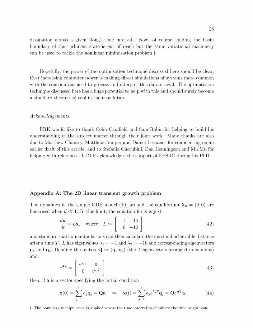
The dynamics in the simple ODE model (10) around the equilibrium X0 = (0, 0) are

linearised when d� 1. In this limit, the equation for x is just

dx

dt= Lx, where L :=

[−1 10

0 −10

](42)

and standard matrix manipulations can then calculate the maximal achievable distance

after a time T . L has eigenvalues λ1 = −1 and λ2 = −10 and corresponding eigenvectors

q1 and q2. Defining the matrix Q := (q1|q2) (the 2 eigenvectors arranged in columns)

and

eΛT =

[eλ1T 0

0 eλ2T

](43)

then, if a is a vector specifying the initial condition

x(0) =2∑j=1

ajqj = Qa ⇒ x(t) =2∑j=1

ajeλjTqj = QeΛTa. (44)

† The boundary manipulation is applied across the time interval to eliminate the time origin issue.

27

0 0.5 1 1.5 20

0.2

0.4

0.6

0.8

1

1.2

1.4

G

ρstart

ρfinish

ρ+

ρ−

T

ρ&

G

Figure 8. The maximum gain G (thick red line) against target time T for the

linear system (42). The thinner solid/dashed blue lines indicate the starting/finishing

values of ρ := x2/x1 for the corresponding optimal. Also shown as horizontal (black)

dotted lines are the orientations where energy growth starts (ρ+) and finishes (ρ− ) (ρ

decreases in time for x2(0) > 0). Notice that the maximum growth occurs precisely

when the initial condition has ρ(0) = ρ+ and T is such that ρ(T ) = ρ−.

Then maxL := Gd2 where the gain

G(T ) = maxa

‖x(T )‖22‖x(0)‖22

= maxa

a†eΛTQ†QeΛTa

a†Q†Qa= ‖M‖22 (45)

and M := QeΛTQ−1 († indicating transpose). G is therefore the largest singular value

of M or equivalently the largest (real) eigenvalue of the symmetric matrix M†M. The

linear optimal θ = θ∗ increases monotonically from 0.1413 (25.4o) at T = 0, through

0.2322 (41.8o) at T=0.16615 where G peaks at 1.26590, and then onto 0.2667 (48.0o)

where G→ 0 as T →∞: see Figure 8.

In 2D, the situation is sufficiently simple to analyse completely for the general linear

problem

dx

dt= Lx :=

[−a b

0 −c

]x (46)

with a, b and c all positive real numbers (the interesting stable case). Defining ρ(t)

as the orientation x2(t)/x1(t) and energy E(t) := 12x(t)2, energy growth begins at the

28

orientation ρ+ and ends at the orientation ρ− where

ρ± :=b±√b2 − 4ac

2c. (47)

The eigenvalues of L are −a and −c and with their corresponding eigenvectors, the

general solution to (46) can be written down as

x(t) = α

[1

0

]e−at + β

[b/(a− c)

1

]e−ct. (48)

Imposing the conditions that ρ(0) = ρ+ and ρ(T ) = ρ− requires

β

α=

ρ+(c− a)

c− a+ bρ+, T ∗ :=

1

c− alog[(ρ+

ρ−

)c− a+ bρ−

c− a+ bρ+

](49)

so that

Gmax =ρ+2(ρ−2 + 1)

ρ−2(ρ+2 + 1)e−2cT

∗. (50)

Appendix B: Linear versus nonlinear transient growth

Here we discuss how nonlinear optimal perturbations are related to linear optimal

perturbations when the nonlinearity in the system preserves the functional being

optimised (a prime example being the energy-preserving nonlinearity of the Navier-

Stokes equations in fluid mechanics). Consider an ODE system whose phase space

is partitioned into subspaces each of which is invariant under the linearised dynamics

about the origin x = 0 which is a stable fixed point. If some of the subspaces support

transient growth then it is possible for nonlinearities in the system to couple these

growth processes to give much larger overall growth than any possible in the linearised

dynamics. To illustrate this, we take a simple 4D system which has two such subspaces,

x :=dx

dt=

−a b 0 0

0 −c 0 0

0 0 −εa εb

0 0 0 −εc

x +

−x1x4

0

0

x21

. (51)

For simplicity, the linear dynamics in each subspace are identical up to a change in

timescale which means that the same maximum transient growth ( Gmax given by (50) )

occurs in both subspaces but at two different times (given by (49) ); T ∗ for subspace

U1 := {(x1, x2, 0, 0) |x1, x2 ∈ R} and T ∗/ε for subspace U2 := {(0, 0, x3, x4) |x3, x4 ∈ R}:see Figure 9. Minimal nonlinear terms are included designed to a) conserve energy (as

in the Navier-Stokes equations) and b) to allow the faster energy growth in subspace

U1 to pump-prime the slower growth in subspace U2. This is clearly seen to occur for δ

large enough when taking the optimal initial condition for U1

x(0) = (x1, x2, x3, x4) = δ(1, ρ+, 0, 0), (52)

see Figure 9 for an example using (a, b, c, ε) = (1, 10, 2, 0.1) (for the linear problem in

U1, Gmax = 6.57 and T ∗ = 0.66).

29

0 1 2 3 4 5 6 7 80

5

10

15

20

25

30

35

40

45

50E

(t)/

E0

t

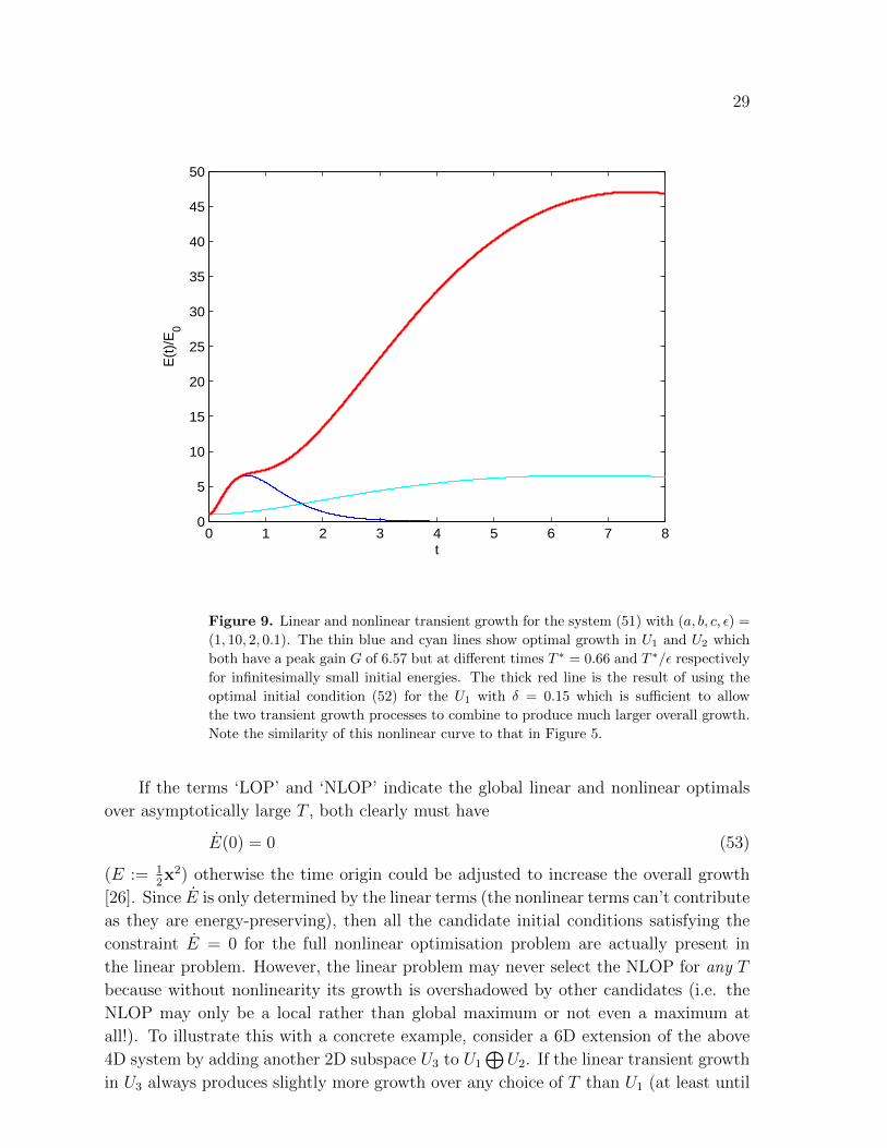
Figure 9. Linear and nonlinear transient growth for the system (51) with (a, b, c, ε) =

(1, 10, 2, 0.1). The thin blue and cyan lines show optimal growth in U1 and U2 which

both have a peak gain G of 6.57 but at different times T ∗ = 0.66 and T ∗/ε respectively

for infinitesimally small initial energies. The thick red line is the result of using the

optimal initial condition (52) for the U1 with δ = 0.15 which is sufficient to allow

the two transient growth processes to combine to produce much larger overall growth.

Note the similarity of this nonlinear curve to that in Figure 5.

If the terms ‘LOP’ and ‘NLOP’ indicate the global linear and nonlinear optimals

over asymptotically large T , both clearly must have

E(0) = 0 (53)

(E := 12x2) otherwise the time origin could be adjusted to increase the overall growth

[26]. Since E is only determined by the linear terms (the nonlinear terms can’t contribute

as they are energy-preserving), then all the candidate initial conditions satisfying the

constraint E = 0 for the full nonlinear optimisation problem are actually present in

the linear problem. However, the linear problem may never select the NLOP for any T

because without nonlinearity its growth is overshadowed by other candidates (i.e. the

NLOP may only be a local rather than global maximum or not even a maximum at

all!). To illustrate this with a concrete example, consider a 6D extension of the above

4D system by adding another 2D subspace U3 to U1

⊕U2. If the linear transient growth

in U3 always produces slightly more growth over any choice of T than U1 (at least until

30

the slower growth in U2 takes over), the linear optimisation problem will never select

any candidate initial condition which has some projection in U1. In contrast the NLOP

will be the linear optimal for U1 (i.e. (52) ) since this is the only way E(0) vanishes

non-trivially in U1. This situation is borne out by the NLOP found in (very high

dimensional) pipe flow [104, 105]. In just 2D, however, there are only two candidates in

the linear problem which are joint global optimisers. Hence in this case the NLOP has

to be contained in the linear problem trivially.

References

[1] Alexakis A 2011 Searching for the fastest dynamo: laminar ABC flows Phys. Rev. E 84 026321.

[2] Andersson P, Berggren M and Henningson D S 1999 Optimal disturbances and bypass transition

in boundary layers Phys. Fluids 11 134-150.

[3] Babloyantz A and Destexhe A 1986 A low-dimensional chaos in an instance of epilepsy Proc. Natl.

Acad. Sci. 83 3513-3517

[4] Baggett J S and Trefethen L N 1995 Low-dimensional models of subcritical transition to turbulence

Phys. Fluids 9 1043-1053.

[5] Baggett J S, Driscoll T A and Trefethen L N 1997 A mostly linear-model of transition to turbulence

Phys. Fluids 7 833-838.

[6] Barkmeijer J 1996 Constructing fast-growing perturbations for the nonlinear regime J. Atmos.

Sci. 53 2838-2851.

[7] Bennett A F 1992 Inverse Methods in Physical Oceanography Cambridge University Press.

[8] Berggren M 1998 Numerical solution of a flow-control problem: vorticity reduction by dynamic

boundary action Siam J. Sci. Comput. 19 829-860.

[9] Bewley T R, Moin P and Temam R 2001 DNS-based predictive control of turbulence: an optimal

benchmark for feedback algorithms J. Fluid Mech. 447 179-225.

[10] Biau D and Bottaro A 2004 Transient growth and minimal defects: two possible initial paths of

transition to turbulence in plane shear flows Phys. Fluids 16 3515-3529.

[11] Biau D and Bottaro A 2009 An optimal path to transition in a duct Phil. Trans. Roy. Soc. Lond.

A 367 529-544.

[12] Boberg L and Brosa U 1988 Onset of turbulence in a pipe Z. Naturforsch. 43a 697-726.

[13] Bottaro A, Corbett P and Luchini P 2003 The effect of base flow variation on flow instability J.

Fluid Mech. 596 113-142.

[14] Buizza R and Palmer T N 1995 The singular-vector structure of the atmospheric global circulation

J. Atmos. Sci. 52 1434-1456.

[15] Butler K M and Farrell B F 1992 3-Dimensional optimal perturbations in viscous shear-flow Phys.

Fluids 4 1637-1650.

[16] Cantwell C D, Barkley D and Blackburn H M 2010 Transient growth analysis of flow through a

sudden expansion in a circular pipe Phys. Fluids 22 034101.

[17] Chandrasekhar S 1961 Hydrodynamic and Hydromagnetic Instability, Oxford University Press.

[18] Cherubini S, De Palma P, Robinet J-C and Bottaro A 2010 Rapid path to transition via nonlinear

localised optimal perturbations in a boundary layer flow Phys. Rev. E 82 066302.

[19] Cherubini S, De Palma P, Robinet J-C and Bottaro A 2011 The minimal seed of turbulent transition

in the boundary layer J. Fluid Mech. 689 221-253.

[20] Cherubini S, De Palma P, Robinet J-C and Bottaro A 2012 A purely nonlinear route to transition

approaching the edge of chaos in a boundary layer Fluid Dynam. Res. 44 031404.

[21] Cherubini S and De Palma P 2013 Nonlinear optimal perturbations in a Couette flow: bursting

and transition J. Fluid Mech. 716 251-279.

31

[22] Cherubini S, Robinet J-C and De Palma P 2013 Nonlinear control of unsteady finite-amplitude

perturbations in the Blasius boundary-layer flow J. Fluid Mech. 737 440-465

[23] Chevalier M, Hogberg M, Berggren M and Henningson D S 2002 Linear and nonlinear optimal

control in spatial boundary layers AIAA paper 2002-2755.

[24] Childress S 1970 New solutions of the kinematic dynamo problem J. Math Phys. 11 3063-3076

[25] Corbett P and Bottaro A 2000 Optimal perturbations for boundary layers subject to streamwise

pressure gradient Phys. Fluids 12 120-130.

[26] Cossu C 2005 An optimality condition on the minimum energy threshold in subcritical instabilities

C. R. Mecanique 333 331-336.

[27] Cossu C, Chevalier, M and Henningson, D S 2007 Optimal secondary energy growth in a plane

channel flow Phys. Fluids 19 058107.

[28] Cossu C, Brandt L, Bagheri, S and Henningson, D S 2011 Secondary threshold amplitudes for

sinuous streak breakdown Phys. Fluids 23 074103.

[29] Cvitanovic P and Gibson J F 2010 Geometry of turbulence in wall-bounded shear flows: periodic

orbits Phys. Scr. 142 014007.

[30] Dauchot O and Manneville P 1997 Local versus global concepts in hydrodynamic stability theory

J. Phys. II France 7 371-389.

[31] Daley R 1991 Atmospheric data analysis Cambridge University Press.

[32] Drazin P G 2002 Introduction to Hydrodynamic Stability Cambridge University Press.

[33] Drazin P G and Reid W H 1981 Hydrodynamic Stability Cambridge University Press.

[34] Duan W, Yu Y, Xu H and Zhao P 2013 Behaviors of nonlinearities modulating the El Nino events

indcued by optimal precursory disturbances Clim. Dyn. 40 1399-1413.

[35] Duan W and Zhou F 2013 Non-linear forcing singular vector of a two-dimensional quasi-geostrophic

model Tellus 65 18452.

[36] Duguet Y, Brandt L and Larsson B R J 2010 Towards minimal perturbations in transitional plane

Couette flow Phys. Rev. E 82 026316.

[37] Duguet Y, Monokrousos A, Brandt L and Henningson D S 2013 Minimal transition thresholds in

plane Couette flow Phys. Fluids 25 084103.

[38] Eckhardt B, Faisst H, Schmeigel A and Schumacher J 2002 Turbulence transition in shear flows.

Advances in Turbulence IX: Proceedings 9th European Turbulence Conference (Southampton)

(ed. I. P. Castro et al.), p701, CISME.

[39] Eckhardt B, Schneider T M, Hof B and Westerweel J 2007 Turbulence transition in pipe flow Ann.

Rev. Fluid Mech. 39 447-468.

[40] Ellingsen T and Palm E 1975 Stability of linear flow Phys. Fluids 18 487-.

[41] Ergaber H, Lenstra D, Krauskopf B, Wille E, Peil M, Fischer I and Elsasser W 2005 Mutually

delay-coupled semiconductor lasers: Mode bifurcation scenarios Opt. Commun. 255 286-296.

[42] Faisst H and Eckhardt B 2004 Sensitive dependence on initial conditions in transition to turbulence

in pipe flow J. Fluid Mech. 504 343-352.

[43] Farrell B F 1988 Optimal excitation of perturbations in viscous shear flow Phys. Fluids 31 2093-

2101.

[44] Farrell B F 1989 Optimal excitation of baroclinic waves J. Atmos. Sci. 46 1193-1206.

[45] Farrell B F 1990 Small error dynamics and the predicability of atmospheric flows J. Atmos. Sci.

47 2409-2416.

[46] Freidlin M I and Wentzell A D 1998 Random Perturbations of Dynamical Systems Springer-Verlag,

New York.

[47] Foures D P G, Caulfield C P and Schmid P J 2012 Variational framework for flow optimisation

using seminorm constraints Phys. Rev E 86 026306.

[48] Foures D P G, Caulfield C P and Schmid P J 2013 Localisation of flow structures using ∞-norm

optimisation J. Fluid Mech. 729 672-701.

[49] Foures D P G, Caulfield C P and Schmid P J 2014 Optimal mixing in two-dimensional plane

Poiseuille flow at high Peclet number J. Fluid Mech. 748, 241-277.

32

[50] Fournier A, Hulot G, Jault D, Kuang W, Tangborn A, Gillet N, Canet E, Aubert J and Lhuillier

F 2010 An introduction to data assimilation and predictability in geomagnetism Space Sci. Rev.

155 247-291.

[51] Gad-el-Hak M 2000 Flow Control: Passive, Active and Reactive Flow Management, Cambridge.

[52] Gavarini M I, Bottaro A and Nieuwstadt F T M 2004 The initial stage of transition in pipe flow:

rle of optimal base-flow distortions J. Fluid Mech. 517 131-165.

[53] Gibson J F, Halcrow J and Cvitanovic P 2008 Visualizing the geometry of state space in plane

Couette flow J. Fluid Mech. 611, 107-130.

[54] Grossmann S 2000 The onset of shear flow turbulence Rev. Mod. Phys. 72 603-618.

[55] Guegan A, Schmid P J and Huerre P 2006 Optimal energy growth and optimal control in swept

Hiemenz flow J. Fluid Mech. 566 11-45.

[56] Gunzburger M 2000 Adjoint equation-based methods for control problems in incompressible,

viscous flows Flow, Turbulence and Combustion 65 249-272.

[57] Gustavsson L H 1991 Energy growth of 3-dimensional disturbances in plane Poiseuille flow J. Fluid

Mech. 224 241-260.

[58] Heisenberg W 1924 Uber stabilitat und turbulenz von flussigkeitsstromen Ann. Phys. Lpz. 74

577-627.

[59] Hinze M, Walther A and Sternberg J 2006 An optimal memory-reduced procedure for calculating

adjoints of the instationary Navier-Stokes equations Optim. Control Appl. Methods 27 19-40.

[60] Hoepffner J, Brandt L and Henningson D S 2005 Transient growth on boundary layer streaks J.

Fluid Mech. 537 91-100.

[61] Hopf E 1948 A mathematical example displaying features of turbulence Commun. Appl. Maths 1,

303-322.

[62] Hultgren L S and Gustavsson L H 1981 Algebraic growth of disturbances in a laminar boundary-

layer Phys. Fluids 24 1000-1004.

[63] Itano T and Toh S 2001 The dynamics of bursting process in wall turbulence J. Phys. Soc. Japan

70 703-716.

[64] Jegadeesan V and Sujith R I 2013 Experimental investigation of noise induced triggering in

thermoacoustic systems Proceedings of the Combustion Institute 34 3175-3183.

[65] Jiang Z and Wang D 2010 A study on precursors to blocking anomalies in climatological flows by

using conditional nonlinear optimal perturbations Quart. J. Roy. Meteor. Soc. 136 1170-1180.

[66] Jiang Z N, Mu M and Luo D H 2013 A study of the North Atlantic Oscillation using conditional

nonlinear optimal perturbation J. Atmos. Sci. 70 855-875.

[67] Joslin R, Gunzburger M D , Nicolaides R A, Erlebacher G and Hussaini M Y 1995 Self-contained

automated methodology for optimal flow control Institute for Computer Applications in Science

and Engineering (ICASE) technical report 95-64.

[68] Joslin R D, Gunzburger M D , Nicolaides R A, Erlebacher G and Hussaini M Y 1997 Self-contained

automated methodology for optimal flow control validated for transition delay AIAA Journal

35 816-824.

[69] Juniper M P 2011 Triggering in the horizontal Rijke tube: non-normality, transient growth and

bypass transition J. Fluid Mech. 667 272-308

[70] Juniper M P 2011 Transient growth and triggering in the horizontal Rijke tube Int. J. Spray and

Combustion Dynamics 3 209-224.

[71] Kalnay E 2003 Atmospheric Modelling, Data Assimilation and Predictability Cambridge University

Press.

[72] Kawahara G, Uhlmann M and van Veen L 2012 The significance of simple invariant solutions in

turbulent flows Ann. Rev. Fluid Mech. 44 203-225.

[73] Kerswell R R 2005 Recent progress in understanding the transition to turbuelnce in a pipe

Nonlinearity 18 R17-R44.

[74] Kerswell R R 2011 Lecture 9: Triggering Transitions - Towards Minimal Seeds, Summer program

in Geophysical Fluid Dynamics, Woods Hole Oceanographic Institute, Massachusetts, USA

33

(http://www.whoi.edu/main//gfd/proceedings-volumes/2011)

[75] Kim J and Bewley T R 2007 A linear systems approach to flow control Ann. Rev. Fluid Mech. 39

383-417.

[76] Kitson S and Geisow A 2002 Controllable alignment of nemantic liquid crystals around microscopic

posts: stabilization of multiple states Appl. Phys. Lett. 80 3635-3637.

[77] Landahl M T 1980 A note on an algebraic instability of inviscid parallel shear flows J. Fluid Mech.

98 243-.

[78] Landau L D 1944 On the problem of turbulence C.R. Acad. Sci. U.R.S.S. 44 311-314.

[79] Lecoanet D and Kerswell R 2013 Nonlinear optimization of multiple perturba-

tions and stochastic forcing of subcritical ODE systems Bull. Am. Phys. Soc. 58

http://meetings.aps.org/link/BAPS.2013.DFD.L10.4

[80] Lorenz E N 1965 A study of the predicability of a 28-variable atmosphere model Tellus 17 321-333.

[81] Luchini P and Bottaro A 1998 Gortler vortices: a backward-in-time approach to the receptivity

problem J. Fluid Mech. 363 1-23.

[82] Luchini P 2000 Reynolds-number-independent instability of the boundary layer over a flat surface:

optimal perturbations J. Fluid Mech. 404 289-309

[83] Luchini P and Bottaro A 2014 Adjoint equations in stability analysis Ann. Rev. Fluid Mech. 46

493-517.

[84] Machowski J, Bialek J W and Bumby J R 2008 Power System Dynamics: Stability and Control,

Wiley.

[85] Menck P J, Heitzig J, Marwan N and Kurths J 2013 How basin stability complements the linear-

stability paradigm Nature Phys. 9 89-92.

[86] Monokrousos A, Bottaro A, Brandt L, Di Vita A and Henningson D S 2011 Nonequilibrium

thermodynamics and the optimal path to turbulence in shear flows Phys. Rev. Lett. 106 134502.

[87] Mu M 2000 Nonlinear singular vectors and nonlinear singular values Sci. China 43D 375-385.

[88] Mu M, Duan W S and Wang B 2003 Conditional nonlinear optimal perturbation and its

applications Nonlin. Processes Geophys. 10 493-501.

[89] Mu M, Sun L and Dijstra H A 2004 The sensitivity and stability of the ocean’s thermohaline

circulation to finite-amplitude perturbations J. Phys. Ocean. 34 2305-2315.

[90] Mu M and Zhang Z 2006 Conditional nonlinear optimal perturbations of a two-dimensional

quasigeostrophic model J. Atmos. Sci. 63 1587-1604.

[91] Mu M and Jiang Z N 2008 A new approach to the generation of initial perturbations for ensemble

prediction using dynamically conditional perturbations Chinese Sci. Bull. 53, 2062-2068.

[92] Mu M and Jiang Z 2008 A method to find perturbations that trigger blocking onset: conditional

nonlinear optimal perturbations Am. Meteor. Soc. 65 3935-3946.

[93] Mu M, Duan W, Wang Q and Zhang R 2010 An extension of conditional optimal perturbation

approach and its applications Nonlin. Proc. Geophys. 17 211-220.

[94] Mu M and Jiang Z 2011 Similarities between optimal precursors that trigger the onset of blocking

events and optimally growing initial errors in onset prediction J. Atmos. Sci. 68 2860-2877.

[95] Mu M, Yu Y S, Xu H and Gong T T 2013 Similarities between optimal precusrosrs for ENSO

events and optimally growing initial errors in El Nino predictions Theor. Appl. Climatol. 115

461-469.

[96] Mullin T 2011 Experimental Studies of Transition to Turbulence in a Pipe Ann. Rev. Fluid Mech.

43 1-24.

[97] Noether F 1921 Das turbulenz problem Z. angew. Math. Mech. 1 125-138.

[98] Oortwijn J and Barkmeijer J 1995 Perturbations that optimally trigger weather regimes J. Atmos.

Sci. 52 3932-3944.

[99] Orr W M 1907 The stability or instability of the steady motions of a perfect fluid and of a viscous

fluid. Part I. A perfect fluid. Part II A viscous fluid Proc. Roy. Irish Acad. 27 9-138.

[100] Palmer T, Molteni F, Mureau R, Buizza R, Chapelet P and Tribbia J 1993 Ensemble prediction

Proc. ECMWF Seminar 1 Reading, UK ECMWF 21-66.

34

[101] Passaggia P-Y and Ehrenstein U 2013 Adjoint based optimisation and control of a separated

boundary-layer flow Eur. J. Mech. B 41 169-177.

[102] Peixinho J and Mullin T 2007 Finite amplitude thresholds for transition in pipe flow J. Fluid

Mech. 582 169-178.

[103] Pralits J O, Hanifi A and Henningson D S 2002 Adjoint-based optimization of steady suction for

disturbance control in incompressible flows J. Fluid Mech. 467 129-161.

[104] Pringle C C T and Kerswell R R 2010 Using nonlinear transient growth to construct the minimal

seed for shear flow turbulence Phys. Rev. Lett. 105 154502.

[105] Pringle C C T, Willis A P and Kerswell R R 2012 Minimal seeds for shear flow turbulence: using

nonlinear transient growth to touch the edge of chaos J. Fluid Mech. 702 415-443.

[106] Pringle C C T, Willis A P and Kerswell R R 2014 Fully localised nonlinear energy growth optimals

in pipe flow Phys. Fluids in preparation.

[107] Rabin S M E A variational approach to determining nonlinear optimal perturbations and minimal

seeds PhD thesis, University of Cambridge, 2013.

[108] Rabin S M E, Caulfield C P and Kerswell R R 2012 Variational identification of minimal seeds

to trigger transition in plane Couette flow J. Fluid Mech. 712 244-272.

[109] Rabin S M E, Caulfield C P and Kerswell R R 2014 Designing a more nonlinearly stable laminar

flow via boundary manipulation J. Fluid Mech. 738 R1.

[110] Rayleigh Lord 1880 On the stability, or instability, of certain fluid motions Proc. London Math.

Soc. 11 57-70.

[111] Reddy S C and Henningson D S 1993 Energy growth in viscous channel flows J. Fluid Mech. 252

209-238.

[112] Reddy S C, Schmid P J, Baggett J S and Henningson D S 1998 On stability of streamwise streaks

and transition thresholds in plane channel flows J. Fluid Mech. 365 269-303.

[113] Reshotko E 2001 Transient growth: a factor in bypass transition Phys. Fluids 13 1067-1075.

[114] Reynolds O 1883a An experimental investigation of the circumstances which determine whether

the motion of water shall be direct or sinuous and of the law of resistance in parallel channels

Proc. R. Soc. Lond. Ser. A 35 84-99.

[115] Reynolds 0 1883b An experimental investigation of the circumstances which determine whether

the motion of water shall be direct or sinuous and of the law of resistance in parallel channels

Phil. Trans. R. Soc. Lond. Ser. A 174 935-982.

[116] Schmid P J 2007 Nonmodal Stability Theory Ann. Rev. Fluid Mech. 39 129-62.

[117] Schmid P J and Henningson D S 2001 Stability and Transition in Shear Flows Springer-Verlag,

New York.

[118] Schmid P J and Brandt L 2014 Analysis of fluid systems: stability, receptivity, sensitivity Appl.

Mech. Rev. 66 024803.

[119] Schneider T M, Eckhardt B and Yorke J A 2007 Turbulence transition and the edge of chaos in

pipe flow Phys. Rev. Lett. 99 034502.

[120] Schneider T M, De Lillo F, Buerhrle J, Eckhardt B, Dornemann T, Dornemann K, Freisleben B

2010 Transient turbulence in plane Couette flow Phys. Rev. E 81 015301.

[121] Schneider T M, Marinc D and Eckhardt B Localized edge states nucleate turbulence in extended

plane Couette cells J. Fluid Mech. 646, 441-451.

[122] Schoppa W and Hussain F 2002 Coherent structure generation in near-wall turbulence J. Fluid

Mech. 453 57-108.

[123] Skufca J D, Yorke J A and Eckhardt B 2006 Edge of chaos in a parallel shear flow Phys. Rev.

Lett. 96 174101.

[124] Sommerfeld A 1908 Ein Beitrag zur hydrodynamischen erklaerung der turbulenten Fluessigkeits-

bewegungen Proceedings 4th International Congress of Mathematicians Rome III 116-124.

[125] Taylor G I Stability of a viscous liquid contained between two rotating cylinders Phil. Trans.

Roy. Soc. Lond. 223 289-343.

[126] Terwisscha van Scheltinga A D and Dijkstra H A 2008 Conditional nonlinear optimal

35

perturbations of the double-gyre ocean circulation Nonlin. Processes Geophys. 15 727-734.

[127] Thomson W (Lord Kelvin) 1887 Stability of fluid motion - rectilineal motion of viscous fluid

between two parallel plates Philos. Mag. 24 188-.

[128] Toth Z and Kalnay E 1993 Ensemble forecasting at NMC: The generation of perturbations Bull.

Amer. Meteor. Soc. 74, 2317-2330.

[129] Toth Z and Kalnay E 1997 Ensemble forecasting at NCEP and the breeding method Am. Meteor.

Soc. 125 5297-3319.

[130] Trefethen L N, Trefethen A E, Reddy S C and Driscoll T A 1993 Hydrodynamic stability without

eigenvalues Science 261 578-584.

[131] Trefethen L N and Embree M 2005 Spectra and Pseudospectra Princeton Uuniversity Press.

[132] Viswanath D and Cvitanovic P 2009 Stable manifolds and the transition to turbulence in pipe

flow J. Fluid Mech. 627 215-233.

[133] Waleffe F 1995 Transition in shear flows: nonlinear normality versus non-normal linearity Phys.

Fluids 7 3060-3066.

[134] Wang Q, Mu M and Dijkstra H A 2012 Application of the conditional nonlinear optimal

perturbation method to the predictability study of the Kuroshio Large Meander Adv. Atmos.

Sci. 29 118-134.

[135] Wang Q, Mu M and Dijkstra H A 2013 Effects of nonlinear physical processes on optimal error

growth in predictability experiments of the Kuroshio large meander J. Geophys. Res. 118 6425-

6436.

[136] Waugh I C and Juniper M P 2011 Triggering in a thermoacoustic system with stochastic noise

Int. J. Spray and Combustion Dynamics 3 225-242.

[137] Willis A P 2012 On the optimised magnetic dynamo Phys. Rev. Lett. 109 251101.

[138] Yu YS, Duan WS, Xu H and Mu M 2009 Dyanmics of nonlinear error growth and season-

dependent predictability of El Nino events in the Zebiak-Cane model Quart. J. Roy. Meteor.

Soc. 135 2146-2160.

[139] Zikanov O Y 1996 On the instability of pipe Poiseuille flow Phys. Fluids 8 2923-2932.

[140] Ziqing Z U, Mu M and Dijkstra H A 2013 Optimal nonlinear excitation of decadal variability of

the North Atlantic thermohaline circulation Chinese J. Ocean. Limnology 31 1356-1362.

[141] Zuccher S, Luchini P and Bottaro A 2004 Algebraic growth in a Blasius boundary layer: optimal

and robust control by mean suction in the nonlinear regime J. Fluid Mech. 513 135-160.

[142] Zuccher S, Bottaro A and Luchini P 2006 Algebraic growth in a Blasius boundary layer: Nonlinear

optimal disturbances Eur. J. Mech. B 25 1-17.