An optimal trading problem in intraday electricity markets ∗

René Aïd † Pierre Gruet ‡ Huyên Pham §

January 20, 2015

Abstract

We consider the problem of optimal trading for a power producer in the contextof intraday electricity markets. The aim is to minimize the imbalance cost induced bythe random residual demand in electricity, i.e. the consumption from the clients minusthe production from renewable energy. For a simple linear price impact model and aquadratic criterion, we explicitly obtain approximate optimal strategies in the intradaymarket and thermal power generation, and exhibit some remarkable properties of thetrading rate. Furthermore, we study the case when there are jumps on the demandforecast and on the intraday price, typically due to error in the prediction of wind powergeneration. Finally, we solve the problem when taking into account delay constraintsin thermal power production.

JEL Classification: G11, Q02, Q40

MSC Classification: 35Q93, 49J20, 60H30, 91G80.

Key words: Optimal trading, power plant, intraday electricity markets, renewable energy,market impact, linear-quadratic control problem, jumps, delay.

∗This study was supported by FiME (Finance for Energy Market Research Centre) and the “Finance etDéveloppement Durable - Approches Quantitatives” EDF - CACIB Chair. The authors would like to thankMarc Ringeisen, Head of EDF R&D Osiris Department for insightful discussion on trading and intradaymarket.†EDF R&D and Finance for Energy Market Research Centre www.fime-lab.org, rene.aid at edf.fr‡LPMA, Université Paris Diderot, gruet at math.univ-paris-diderot.fr§LPMA, Université Paris-Diderot and CREST-ENSAE, pham at math.univ-paris-diderot.fr

1

arX

iv:1

501.

0457

5v1

[q-

fin.

TR

] 1

9 Ja

n 20

15

1 Introduction

The development of renewable energy sources in Europe as a response to global climatechange has led to an increase of exchange in the intraday electricity markets. For instance,the exchanged volume on the European Energy Exchange (EEX) for Germany has grownfrom 2 TWh in 2008 to 25 TWh in 2013. This increase is mainly due to the level offorecasting error of wind production, which leads power producers owning a large share ofwind production to turn more than ever to intraday markets in order to adjust their positionand avoid penalties for their imbalances. The accuracy of forecasts for renewable powerproduction from wind and solar may vary considerably depending on the agreggation level(local vs regional forecast) and the time horizon. For a complete survey on this problem, thereader can consult Giebel et al. [5], and may have in mind that the root mean square error(RMSE) of the error forecast for the production of a wind farm in six hours can reach 20% ofits installed capacity. Many different intraday markets have been designed and are subjectto different sets of regulation. But, in all cases, intraday markets offer power producer thepossibility to buy or sell power for the next (say) 9 hours to 32 hours (case of the Frenchelectricity market of EpexSpot). These trades can occur after the closing of the day-aheadmarket or during the clearing phase of the day-ahead market.

The problem of trading management in the intraday electricity market for a balancingpurpose has already drawn the attention in the literature. Henriot [6] studied the problemof how the intraday market can help a power producer to deal with the wind productionerror forecast in a stylized discrete time model. In his model, the power producer is awind producer who is trying to minimize her sourcing cost on the intraday market whilemaintaining a balance position between her forecast production and her sales. Henriot’smodel takes into account the impact of the wind power producer on the intraday price witha deterministic inverse demand function, and the intraday price is not a risk factor. The onlyrisk factor comes from the error forecast of the wind production and its auto-correlation.Garnier and Madlener [4] studies the trade-off between entering into a deal in the intradaymarket right now and postponing it in a discrete time decision model where intraday pricesfollow a geometric Brownian model and wind production error forecast follows an arithmeticBrownian motion. In their framework, the power producer is supposed to have no impacton intraday prices. Liquidity risk is taken into account as a probability of not finding acounter-party at the next trading window.

In this paper, we consider a power producer having at disposal some renewable energysources (e.g. wind and solar), and thermal plants (e.g. coal, gas, oil, and nuclear sources),and who can buy/sell energy in the intraday markets. Her purpose is to minimize theimbalance cost, i.e. the cost induced by the difference between the demand of her clientsminus the electricity produced and traded, plus the production and trading costs. In contrastwith thermal power plants whose generation can be controlled, the power generated fromrenewable sources is subject to non controllable fluctuations or risks (wind speed, weatherforecast) and is then considered here as a random factor just like the demand. We then callthe residual demand the demand minus the energy generated by renewable energy. Thus, theproblem of the power producer is to minimize the imbalance costs arising from her residualdemand by relying both on her own controllable thermal assets and on the intraday market.As in [4], we assume that the power producer has access to a continuously updated forecastof the residual demand to be satisfied at terminal date T and that this forecast evolvesrandomly. Moreover, the intraday price for delivery at time T evolves also randomly andis correlated with the residual demand forecast. However, compared with [4], the intraday

2

market can be used for optimization purposes. We develop a model that allows us to studyhow power producers can take advantage of the interaction between the dynamics of theresidual demand forecast and the dynamics of the intraday prices.

Our model shares some links with optimal order execution problems, as introduced inthe seminal paper by Almgren and Chriss [2], and then largely studied in the recent lit-erature, see e.g. the survey paper [9]. In our context, the original feature with respectto this literature is the consideration of a random demand target and the possibility forthe agent to use her thermal power production. This connection with optimal executionis fruitful in the sense that it allows us to take into account several features of intradaymarkets while maintaining the tractability of the model sufficiently high to allow analyticalsolutions. Hence, we take into account liquidity risk through a market impact, both perma-nent and temporary, on the electricity price generated by a power producer when tradingin the intraday market. As in optimal execution problems, this impact is always in theadverse direction: when the producer sells, the price decreases and when she buys, the priceincreases. Our setting is a continuous-time decision problem representing the possibility forthe producer to make a deal at each time she wants and not only at pre-specified windows.Moreover, it is general enough as it permits us to study the limiting cases of a pure retailer(no production function), a pure trader (no demand commitment) and an integrated player(player owning both clients and generation), small or large.

The main goal of this paper is to derive analytical results, which provide explicit solutionsfor the (approximate) optimal control, hence giving enlightening economic interpretationsof the optimal trading strategies. In order to achieve such analytical tractability, we haveto make some simplifying assumptions on the dynamics of the price process and of theresidual demand forecast, as well as on the cost function, assumed to be of quadratic formmeaning a simple linear growth of the marginal cost of production with respect to theproduction level. We first consider a simple model for a continuous price process with linearimpact, and demand forecast driven by an arithmetic Brownian motion, and neglect in afirst step the delay of production when using thermal power plants. We then study anauxiliary control problem by relaxing the nonnegativity constraint on the generation level,for which we are able to derive explicit solutions. The approximation error induced by thisrelaxation constraint is analyzed. In next steps, we consider more realistic situations andinvestigate two extensions: (i) On one hand, we incorporate the case where the residualdemand forecast is subject to sudden changes, related to prediction error for wind or solarpower production, which may be quite important due to the difficulties for estimating windspeed and forecasting weather, see [3]. This is formalized by jumps in the dynamics of thedemand process, and consequently also on the price process. Again, we are able to obtainexplicit solutions. Actually, the key tool in the derivation of all these analytical results is asuitable treatment of the linear-quadratic structure of our stochastic control problem. (ii)On the other hand, we introduce natural delay constraints in the production, and show howthe optimal decision problem can be explicitly solved by a suitable reduction to a problemwithout delay.

Our (approximate) optimal trading strategies present some remarkable properties. Whenthe intraday price process is a martingale, the optimal trading rate inherits the martingaleproperty, which implies in particular that the net position of electricity shares has a constantgrowth rate on average. Moreover, the optimal strategy consists in making at each timethe forecast marginal cost equal to the forecast intraday price. This property follows thecommon sense of intraday traders. Consequently, if the producer has made sales or purchases

3

on the day-ahead such that her forecast marginal cost equals the day-ahead price and if theinitial condition of the intraday price is the day-ahead price, thus, on average, the produceroptimal trading rate is zero. This fact is no longer true when the demand forecast and theprice follow processes with jumps. In this case, the optimal trading rate is a supermartingaleor a submartingale depending on the relative probability and size of positive and negativejumps on the price process. For this reason, contrary to the case without jumps, the powerproducer may need to have a non-zero initial trading rate even if she has made sales orpurchases on the day-ahead such that her forecast marginal cost equals the day-ahead priceand if the initial condition of the intraday price is the day-ahead price. We also quantifyexplicitly the impact of delay in production on the trading strategies. When the priceprocess is a martingale, the net inventory in electricity shares grows linearly on average,with a change of slope (which is smaller) at the time decision for the production.

The outline of the paper is organized as follows. We formulate the optimal tradingproblem in Section 2. In Section 3, we study the optimal trading problem without delay.We first solve explicitly the auxiliary optimal execution problem, and then study the ap-proximation on the solution to the original problem, by focusing in particular on the errorasymptotics. We illustrate our results with some numerical tests and simulations. We extendin Section 4 our results to the case where jumps in demand forecast may arise. In Section5, we show how the optimal trading problem with delay in production can be reduced to aproblem without delay, and then leads to explicit solutions. Finally, the appendix collectsthe explicit derivations of our solutions, which are justified by verification theorems.

2 Problem formulation

We consider an agent on an intraday energy market, who is required to guarantee herequilibrium supply/demand for a given fixed time T : she has to satisfy the demand of hercustomers by purchase/sale of energy on the intraday market at time T and also by meansof her thermal power generation. We denote by Xt the net position of sales/purchases ofelectricity at time t ≤ T for a delivery at terminal time T , assumed to be described byan absolutely continuous trajectory up to time T , and by qt = Xt the trading rate: qt >0 means an instantaneous purchase of electricity, while qt < 0 represents an instantaneoussale at time t:

Xt = X0 +

∫ t

0qsds, 0 ≤ t ≤ T. (2.1)

Given the trading rate, the transactions occur with a market price impact:

Pt(q) = Pt +

∫ t

0g(qs)ds+ f(qt).

Here, (Pt)t is the unaffected intraday electricity price process on a filtered probability space(Ω,F ,F = (Ft)t∈[0,T ],P), carrying some part of randomness of the market, and followingthe terminology in the seminal paper by Almgren and Chriss [2], the term f(qt) refers tothe temporary price impact, while

∫ t0 g(qs)ds describes the permanent price impact. The

price (Pt)t may be seen as a forward price, evolving in real time, for delivery at time T . Letus then denote by Y the intraday electricity price impacted by the past trading rate q ofthe agent, defined by:

Yt := Pt +

∫ t

0g(qs)ds.

4

We assume that Yt is observable and quoted, which means actually that the agent is a largetrader and electricity producer, whose actions directly impact the intraday electricity price.The case where the agent is a small producer can be also dealt with by simply consideringa zero permanent impact function g ≡ 0. Notice that the transacted price is equal to thesum of the quoted price Y and the temporary price impact:

Pt(q) = Yt + f(qt). (2.2)

The residual demand DT is the consumption of clients of the agent minus the productionfrom renewable energy at terminal date T , and we assume that the agent has access to acontinuously updated forecast (Dt)t of the residual demand. The agent can use her thermalpower production with a quantity ξ at cost c(ξ) in order to match as close as possible thetarget demandDT . In practice, generation of electricity can not be obtained instantaneouslyand needs a delay to reach a required level of production. Hence, the decision to producea quantity ξ should be taken at time T − h, where h ∈ [0, T ] is the delay. Thus, for acontrolled trading rate q = (qt)t ∈ A, the set of real-valued F-adapted processes satisfyingsome integrability conditions to be precised later, a production quantity ξ ∈ L0

+(FT−h), theset of nonnegative FT−h-measurable random variables, the total cost is:∫ T

0qtPt(q)dt+ C(DT −XT , ξ) :=

∫ T

0qtPt(q)dt+ c(ξ) +

η

2(DT −XT − ξ)2. (2.3)

The first term in (2.3) represents the total running cost arising from the trading in theintraday electricity market, and the last term, where η > 0, represents the quadratic pe-nalization when the net position in sales/purchases of electricity XT + ξ (including theproduction quantity ξ at cost c(ξ)) at terminal date T does not fit the effective demand DT .The objective of the agent is then to minimize over q and ξ the expected total cost:

minimize over q ∈ A, ξ ∈ L0+(FT−h) E

[ ∫ T

0qtPt(q)dt+ C(DT −XT , ξ)

]. (2.4)

Remark 2.1 1) The penalization term in the objective function above is a simplification ofthe effective penalization process that can be found in real electricity markets. For instance,the penalization of imbalances in the French electricity market depends both on the signof the imbalance of the electricity system and on the price of imbalances (see [1, chap 2.,sec. 2.2.1]). Nevertheless, the positive coefficient η captures the main objective of thepenalization process. The agent has no incentive of being either too long or too short.2) On real markets, trading ends some time before the date of delivery, at which the agenthas to ensure equilibrium (e.g. on the French electricity market, there is a delay of 45minutes). We do not include that practical fact in our framework, by considering that thedelay is null for the sake of clarity. There is no mathematical consequence: it is enough tohave in mind that the delivery and production do not really take place at T , but at T plussome delay.3) The larger is η, the stronger is the incentive for the agent to be as close as possibleto the equilibrium supply-demand. At the limit, when η goes to infinity, the agent isformally constrained to fit supply and demand. However, the limiting problem when η =∞ is not mathematically well-posed since such perfect equilibrium constraint is in generalnot achievable. Indeed, the demand at terminal date T is random, typically modelled via aGaussian noise, and the inventoryX which is of finite variation, may exceed or underperform

5

with positive probability the demand DT at terminal date T . Hence, in the scenario whereXT > DT , and since by nature the production quantity ξ is nonnegative, it is not possibleto realize the equilibrium XT + ξ = DT , even if there is no delay. In the sequel, we fix η >0 (which may be large, but finite), and study the stochastic control problem (2.4).4) The optimization problem (2.4) shares somes similarities with the optimal executionproblem in limit order book studied in the seminal paper by Almgren and Chriss [2], andthen extended by many authors in the literature, see e.g. the survey paper [9]. The maindifference is that in the execution problem of equities, the target is to buy or sell a certainnumber of shares, i.e. lead XT to a fixed constant (meaning formally that η goes to infinity)while in our intraday electricity markets context, the target is to realize the equilibrium withthe random demand DT , eventually with the help of production leverage ξ. However, incontrast with the case of constant target, it is not possible in presence of random target DT

to achieve perfectly the equilibrium, which justifies the introduction of the penalty factor ηas pointed out above.

The main aim of this paper is to provide explicit (or at least approximate explicit)solutions to the optimization problem (2.4), which are easily interpreted from an economicpoint of view, and also allow to measure the impact of the various parameters of the model.In order to achieve this goal, we shall adapt our modeling as close as possible to the linear-quadratic framework of stochastic control, and make the following assumptions: The energyproduction cost function is in the quadratic form:

c(x) =β

2x2,

for some β > 0. Although simple, a quadratic cost function represents the increase of themarginal cost of production with the level of production.

Remark 2.2 (Pure retailer) In the limiting case when β goes to infinity, meaning an infi-nite cost of production, this corresponds to the framework where the agent never uses theproduction leverage and only trades in the intraday-market by solving the optimal executionproblem:

minimize over q ∈ A E[ ∫ T

0qtPt(q)dt+ C(DT −XT , 0)

]. (2.5)

As in Almgren and Chriss, we assume that the price impact (both permanent andtemporary) is of linear form, i.e.

g(q) = νq, f(q) = γq,

for some constants ν ≥ 0 and γ > 0. The unaffected intraday electricity price is taken as aBachelier model:

Pt = P0 + σ0Wt, (2.6)

whereW is a standard Brownian motion, and σ0 > 0 is a positive constant. Such assumptionmight seem a shortcoming at first sight since it allows for negative values of the unaffectedprice. However, in practice, for our intraday execution problem within few hours, negative

6

prices occur only with negligible probability. The martingale assumption is also standardin the market impact literature since drift effects can often be ignored due to short tradinghorizon. The quoted price Y , impacted by the past trading rate q ∈ A, is then governed bythe dynamics:

dYt = νqtdt+ σ0dWt. (2.7)

The dynamics of the residual demand forecast is given by

dDt = µdt+ σddBt, (2.8)

where µ, σd are constants, with σd > 0, and B is a Brownian motion correlated with W :d < W,B >t = ρdt, ρ ∈ [−1, 1].

From (2.2), one can then define the value function associated to the dynamic version ofthe optimal execution problem (2.4) by:

v(t, x, y, d) := infq∈At,ξ∈L0

+(FT−h)J(t, x, y, d; q, ξ) (2.9)

with

J(t, x, y, d; q, ξ) := E[ ∫ T

tqs(Y

t,ys + γqs)ds+ C(Dt,d

T −Xt,xT , ξ)2

], (2.10)

for (t, x, y, d) ∈ [0, T ] × R × R × R, where At denotes the set of real-valued processes q =

(qs)t≤s≤T s.t. qs is Fs-adapted and E[ ∫ T

t q2sds] < ∞, Dt,d is the solution to (2.8) startingfrom d at t, and given a control q ∈ At, Y t,y denotes the solution to (2.7) starting from yat time t, and Xt,x is the solution to (2.1) starting from x at t.

In a first step, we shall consider the case when there is no delay in the production, andthen show in the last section of this paper how to reduce the problem with delay to a nodelay problem. We shall also study the case when there are jumps in the residual demandforecast.

3 Optimal execution without delay in production

In this section, we consider the case when there is no delay in production, i.e. h = 0. In thiscase, we notice that the optimization over q and ξ in (2.4) is done separately. Indeed, theproduction quantity ξ ∈ L0

+(FT ) is chosen at the final date T , after the decision over thetrading rate process (qt)t∈[0,T ] is achieved (leading to an inventory XT ). It is determinedoptimally through the optimization a.s. at T of the terminal cost C(DT −XT , ξ), hence infeedback form by ξ∗T = ξ+(DT −XT ) where

ξ+(d) := arg minξ≥0

C(d, ξ) = arg minξ≥0

[β2ξ2 +

η

2(d− ξ)2

]=

η

η + βd1d≥0. (3.1)

The value function of problem (2.9) may then be rewritten as

v(t, x, y, d) = infq∈At

E[ ∫ T

tqs(Y

t,ys + γqs)ds+ C+(Dt,d

T −Xt,xT )2

], (3.2)

7

where

C+(d) := C(d, ξ+(d))

=1

2

ηβ

η + βd21d≥0 +

η

2d21d<0. (3.3)

and the optimal trading rate q∗ is derived by solving (3.2).Due to the indicator function in C+, caused by the non negativity constraint on the

production quantity, there is no hope to get explicit solutions for the problem (3.2), i.e. solveexplicitly the associated dynamic programming Hamilton-Jacobi-Bellman (HJB) equation.We shall then consider an auxiliary execution problem by relaxing the sign constraint on theproduction quantity, for which we are able to provide explicit solution. Next, we shall seehow one can derive an approximate solution to the original problem in terms of this auxiliaryexplicit solution, and we evaluate the error and illustrate the quality of this approximationby numerical tests.

3.1 Auxiliary optimal execution problem

We consider the optimal execution problem with relaxation on the non negativity constraintof the production leverage, and thus introduce the auxiliary value function

v(t, x, y, d) := infq∈A,ξ∈L0(FT )

J(t, x, y, d; q, ξ),

for (t, x, y, d) ∈ [0, T ] × R × R × R. By same arguments as for the derivation of (3.2), wehave

v(t, x, y, d) = infq∈A

E[ ∫ T

tqs(Y

t,ys + γqs)ds+ C(Dt,d

T −Xt,xT )], (3.4)

where

ξ(d) := arg minξ∈R

C(d, ξ) =η

η + βd,

C(d) := C(d, ξ(d)) =1

2

ηβ

η + βd2 =:

1

2r(η, β)d2. (3.5)

The function in (3.5) can be interpreted as a reduced cost function. Because the productioncost function and the penalization are both quadratic, they can be reduced to a singleproduction function where the imbalances are internalized by the producer.

By exploiting the linear-quadratic structure of the stochastic control problem (3.4), wecan obtain explicit solutions for this auxiliary problem.

8

Theorem 3.1 The value function to (3.4) is explicitly equal to:

v(t, x, y, d) =r(η, β)(ν2 (T − t) + γ)

(r(η, β) + ν)(T − t) + 2γ

((d− x)2 + 2µ(T − t)(d− x)

)+

T − t(r(η, β) + ν)(T − t) + 2γ

(− y2

2+ r(η, β)µ(T − t)y

)+

r(η, β)(T − t)(r(η, β) + ν)(T − t) + 2γ

(d− x)y

+ γσ20 + σ2dr

2(η, β)− 2ρσ0σdr(η, β)(r(η, β) + ν

)2 ln(

1 +(r(η, β) + ν)(T − t)

2γ

)+σ2dr(η, β)ν + 2ρσ0σdr(η, β)− σ20

2(r(η, β) + ν

) (T − t)

+r(η, β)µ2(T − t)2(ν2 (T − t) + γ)

(r(η, β) + ν)(T − t) + 2γ,

for (t, x, y, d) ∈ [0, T ]×R×R×R, with an optimal trading rate given in feedback form by:

qs = q(T − s,Dt,d

s − Xt,x,y,ds , Y t,x,y,d

s

), t ≤ s ≤ T

q(t, d, y) :=r(η, β)(µt+ d)− y(r(η, β) + ν)t+ 2γ

. (3.6)

Here (Xt,x,y,d, Y t,x,y,d, Dt,d) denotes the solution to (2.1)-(2.7)-(2.8) when using the feedbackcontrol q, and starting from (x, y, d) at time t. Finally, the optimal production leverage isgiven by:

ξT = ξ(Dt,dT − X

t,x,y,dT ) =

η

η + β

(Dt,dT − X

t,x,y,dT

). (3.7)

Skech of proof. We look for a candidate solution to (3.4) in the quadratic form:

w(t, x, y, d) = A(T − t)(d− x)2 +B(T − t)y2 + F (T − t)(d− x)y

+ G(T − t)(d− x) +H(T − t)y +K(T − t),

for some deterministic functions A, B, F , G, H and K. Plugging this ansatz into theHamilton-Jacobi-Bellman (HJB) equation associated to the stochastic control problem (3.4),we find that these deterministic functions should satisfy a system of Riccati equations, whichcan be explicitly solved. Then, by a classical verification argument, we check that this ansatzw is indeed equal to v, with an optimal feedback control derived from the argmax in theHJB equation. The details of the proof are reported in Appendix.

Remark 3.1 (Pure trader) By sending β to infinity in the expression of the value functionv and of the optimal feedback control q, and observing that r(η, β) goes to η, we obtain the

9

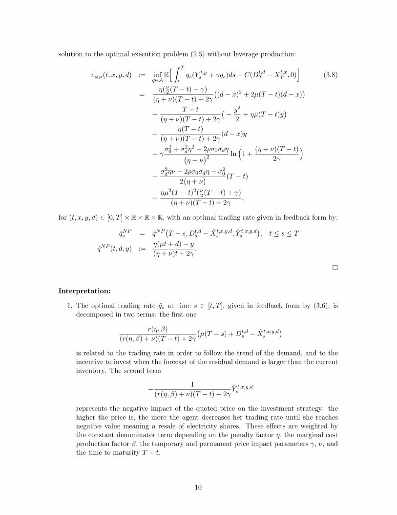
solution to the optimal execution problem (2.5) without leverage production:

vNP (t, x, y, d) := infq∈A

E[ ∫ T

tqs(Y

t,ys + γqs)ds+ C(Dt,d

T −Xt,xT , 0)

](3.8)

=η(ν2 (T − t) + γ)

(η + ν)(T − t) + 2γ

((d− x)2 + 2µ(T − t)(d− x)

)+

T − t(η + ν)(T − t) + 2γ

(− y2

2+ ηµ(T − t)y

)+

η(T − t)(η + ν)(T − t) + 2γ

(d− x)y

+ γσ20 + σ2dη

2 − 2ρσ0σdη(η + ν

)2 ln(

1 +(η + ν)(T − t)

2γ

)+σ2dην + 2ρσ0σdη − σ20

2(η + ν

) (T − t)

+ηµ2(T − t)2(ν2 (T − t) + γ)

(η + ν)(T − t) + 2γ,

for (t, x, y, d) ∈ [0, T ]×R×R×R, with an optimal trading rate given in feedback form by:

qNPs = qNP(T − s,Dt,d

s − Xt,x,y,ds , Y t,x,y,d

s

), t ≤ s ≤ T

qNP (t, d, y) :=η(µt+ d)− y(η + ν)t+ 2γ

.

Interpretation:

1. The optimal trading rate qs at time s ∈ [t, T ], given in feedback form by (3.6), isdecomposed in two terms: the first one

r(η, β)

(r(η, β) + ν)(T − t) + 2γ

(µ(T − s) +Dt,d

s − Xt,x,y,ds

)is related to the trading rate in order to follow the trend of the demand, and to theincentive to invest when the forecast of the residual demand is larger than the currentinventory. The second term

− 1

(r(η, β) + ν)(T − t) + 2γY t,x,y,ds

represents the negative impact of the quoted price on the investment strategy: thehigher the price is, the more the agent decreases her trading rate until she reachesnegative value meaning a resale of electricity shares. These effects are weighted bythe constant denominator term depending on the penalty factor η, the marginal costproduction factor β, the temporary and permanent price impact parameters γ, ν, andthe time to maturity T − t.

10

2. By introducing the marginal cost function: c′(x) = βx, and the process

ξs :=η

η + β

(Dt,ds + µ(T − s)− Xt,x,y,d

s − qs(T − s)), t ≤ s ≤ T,

which is interpreted as the forecast production for the final time T (recall expression(3.7) of the final production), we notice from the expression of the optimal tradingrate that the following relation holds:

Y t,x,y,ds + νqs(T − s) + 2γqs = c′(ξs), t ≤ s ≤ T. (3.9)

This relation means that at each time, the optimal trading rate is to make the forecastintraday price plus marginal temporary impact (left hand side), which can be seen asthe marginal cost of electricity on the intraday market at time T , equal to the forecastmarginal cost of production. Here, the instantaneous impact γ appears as a marginalcost of buying or selling, and the forecast at time s supposes that the optimal tradingrate qs is held constant between s and T .

We complete the description of the optimal trading rate by pointing out a remarkablemartingale property.

Proposition 3.1 The optimal trading rate process (qs)t≤s≤T in (3.6) is a martingale.

Proof. By applying Itô’s formula to qs = q(T − s,Dt,ds − Xt,x,y,d

s , Y t,x,y,ds ), t ≤ s ≤ T , and

since q is linear in d and y, we have:

dqs =[− ∂q

∂t+ (µ− q)∂q

∂d+ νq

∂q

∂y

](T − s,Dt,d

s − Xt,x,y,ds , Y t,x,y,d

s )ds

+∂q

∂d(T − s,Dt,d

s − Xt,x,y,ds , Y t,x,y,d

s )σddBs

+∂q

∂y(T − s,Dt,d

s − Xt,x,y,ds , Y t,x,y,d

s )σ0dWs,

from the dynamics (2.1), (2.8), and (2.7) of Xt,x,y,d, Dt,d and Y t,x,y,d. Now, from the explicitexpression of the function q(t, y, d), we see that

−∂q∂t

+ (µ− q)∂q∂d

+ νq∂q

∂y= 0,

and so:

dqs =r(η, β)σd

(r(η, β) + ν)(T − s) + 2γdBs −

σ0(r(η, β) + ν)(T − s) + 2γ

dWs, (3.10)

which shows the required martingale property.

Remark 3.2 Recall that in the classical optimal execution problem as studied in [2], theoptimal trading rate is constant. We retrieve this result in their framework which corres-ponds to the case where σd = 0 (constant demand target), β = ∞ (there is no production),and η = ∞ (constraint to lead XT to the fixed target), see Remark 2.1 4). Indeed, inthese limiting regimes, we see from (3.10) that dqs = 0, meaning that qs, t ≤ s ≤ T isconstant. In our framework, this is generalized to the martingale property of the optimal

11

trading rate process, which implies that the optimal inventory Xt,x,y,ds , t ≤ s ≤ T has a

constant growth rate in mean, i.e. dE[Xt,x,y,ds ]ds is constant equal to the initial trading rate at

time t given by q(T − t, d− x, y).As a consequence of this martingale property, if the producer already satisfies the relation

(3.9) in the day-ahead market, and if the initial intraday price is the day-ahead price, herinitial trading rate on the intraday market will be zero. And thus, on average, her tradingrate will be zero.

The martingale property of the trading rate process is actually closely related to themartingale dynamics of the unaffected price P in (2.6). As we shall see in Section 4 wherewe consider jumps on price, making P a sub or super martingale, the optimal trading ratewill inherit the converse sub or super martingale property.

3.2 Approximate solution

We go back to the original execution problem with the non negativity constraint on theproduction quantity. As pointed out above, there is no explicit solution in this case, dueto the form of the terminal cost function C+. The strategy is then to use the explicitcontrol consisting in the trading rate q derived in (3.6), and of the truncated nonnegativeproduction quantity:

ξ∗T := ξT1ξT≥0= ξ+(Dt,d

T − Xt,x,y,dT ), (3.11)

with ξT defined in (3.7) from the auxiliary problem. In other words, we follow the tradingrate strategy q determined from the problem without constraint on the final productionquantity, and at the terminal date use the production leverage if the final inventory Xt,x,y,d

T

is below the terminal demand Dt,dT , by choosing a quantity proportional to this spread

Dt,dT − Xt,x,y,d

T . The aim of this section is to measure the relevance of this approximatestrategy (q, ξ∗T ) ∈ A × L0

+(FT ) with respect to the optimal execution problem (2.9) byestimating the induced error:

E1(t, x, y, d) := J(t, x, y, d; q, ξ∗T )− v(t, x, y, d),

for (t, x, y, d) ∈ [0, T ]× R× R× R. We also measure the approximation error on the valuefunctions:

E2(t, x, y, d) := v(t, x, y, d)− v(t, x, y, d).

Notice that if ξT ≥ 0 a.s., i.e. Dt,dT ≥ Xt,x,y,d

T a.s. (which is not true), and so ξ∗T = ξT ,then clearly (q, ξT ) would be the solution to (2.9), and so E1(t, x, y, d) = E2(t, x, y, d) = 0.Actually, these errors depend on the probability of the event: Xt,x,y,d

T > Dt,dT , and we

have the following estimate:

Proposition 3.2 For all (t, x, y, d) ∈ [0, T ]× R× R× R, we have

0 ≤ Ei(t, x, y, d) ≤ ηr(η, β)

2βV (T − t)ψ

(m(T − t, d− x, y)√V (T − t)

), i = 1, 2, (3.12)

where

ψ(z) := (z2 + 1)Φ(−z)− zφ(z), z ∈ R,

12

with φ = Φ′ the density of the standard normal distribution, and

m(t, d, y) :=(νt+ 2γ)(µt+ d) + yt

(r(η, β) + ν)t+ 2γ, (3.13)

V (t) :=

∫ t

0

σ20s2 + σ2d(νs+ 2γ)2 + 2ρσ0σds(νs+ 2γ)[

(r(η, β) + ν)s+ 2γ]2 ds ≥ 0. (3.14)

Proof. By definition of the value functions v and v, recalling that (q, ξT ) is an optimalcontrol for v, and since (q, ξ∗T ) ∈ A× L0

+(FT ), we have:

J(t, x, y, d; q, ξT ) = v(t, x, y, d) ≤ v(t, x, y, d) ≤ J(t, x, y, d; q, ξ∗T ),

for all (t, x, y, d) ∈ [0, T ] × R × R × R. This clearly implies that both errors E1 and E2 arenonnegative, and

max(E1(t, x, y, d), E2(t, x, y, d)) ≤ E(t, x, y, d) := J(t, x, y, d; q, ξ∗T )− J(t, x, y, d; q, ξT ).

We now focus on the upper bound for E . By definition of J in (2.10), ξT and ξ∗T in (3.7)and (3.11), we have

E(t, x, y, d) = E[C(Dt,d

T − Xt,x,y,dT , ξ∗T )− C(Dt,d

T − Xt,x,y,dT , ξT )

]= E

[C(Dt,d

T − Xt,x,y,dT , ξ+(Dt,d

T − Xt,x,y,dT ))

− C(Dt,dT − X

t,x,y,dT , ξ(Dt,d

T − Xt,x,y,dT ))

]= E

[C+(Dt,d

T − Xt,x,y,dT )− C(Dt,d

T − Xt,x,y,dT )

]=

ηr(η, β)

2βE[(Dt,dT − X

t,x,y,dT

)21Dt,dT −X

t,x,y,dT <0

], (3.15)

from the definitions and expressions of C+ and C in (2.3), (3.3) and (3.5). Now, from (3.10)and by integration, we obtain the explicit (path-dependent) form of the optimal tradingrate control:

qs = qt +

∫ s

t

r(η, β)σd(r(η, β) + ν)(T − u) + 2γ

dBu

−∫ s

t

σ0(r(η, β) + ν)(T − u) + 2γ

dWu, t ≤ s ≤ T,

with qt = q(T − t, d − x, y). We then obtain the expression of the final spread betweendemand and inventory:

Dt,dT − X

t,x,y,dT = d− x+ µ(T − t) +

∫ T

tσddBs −

∫ T

tqsds

= m(T − t, d− x, y) +

∫ T

t

σd(ν(T − s) + 2γ)

(r(η, β) + ν)(T − s) + 2γdBs

+

∫ T

t

σ0(T − s)(r(η, β) + ν)(T − s) + 2γ

dWs,

by Fubini’s theorem, and with

m(t, d, y) := d+ µt− tq(t, d, y),

13

which is explicitly written as in (3.13) from the expression (3.6) of q. Thus, Dt,dT − X

t,x,y,dT

follows a normal distribution law with mean m(T − t, d− x, y) and variance V (T − t) givenby (3.14), and from (3.15), we deduce that

E(t, x, y, d) =ηr(η, β)

2βV (T − t)ψ

(m(T − t, d− x, y)√V (T − t)

),

while the probability that the final inventory is larger than the terminal demand is:

P[Dt,dT − X

t,x,y,dT < 0

]= Φ

(− m(T − t, d− x, y)√

V (T − t)

). (3.16)

Error asymptotics. We now investigate the accuracy of the upper bound in (3.12)

E(T − t, d− x, y) :=ηr(η, β)

2βV (T − t)ψ

(m(T − t, d− x, y)√V (T − t)

).

It is well-known (see e.g. Section 14.8 in [10]) that

zΦ(−z) ≤ φ(z), ∀z ∈ R, (3.17)

from which we easily see that ψ is non increasing, convex, and ψ(∞) = 0. Thus, E(T −t, d− x, y) decreases to zero for large m(T − t, d− x; y) or small V (T − t). We shall studyits asymptotics in three limiting cases (i) the time to maturity T − t is small, (ii) the initialdemand spread d − x is large, (iii) the initial quoted price y is large. We prove that theerror bound E(T − t, d− x, y), and thus E1(t, x, y, d), E2(t, x, y, d), converge to zero at leastwith an exponential rate of convergence in these limiting regimes:

Proposition 3.3 (i) For all (x, y, d) ∈ R× R× R with d > x, we have

lim supT−t↓0

(T − t) ln E(T − t, d− x, y) ≤ −1

2

(d− xσd

)2. (3.18)

(ii) For all (t, y) ∈ [0, T )× R, we have

lim supd−x→∞

1

(d− x)2ln E(T − t, d− x, y) ≤ −1

2

m2∞(T − t)V (T − t)

, (3.19)

where

m∞(t) =νt+ 2γ(

r(η, β) + ν)t+ 2γ

(iii) For all (t, x, d) ∈ [0, T )× R× R, we have

lim supy→∞

1

y2ln E(T − t, d− x, y) ≤ −1

2

n2∞(T − t)V (T − t)

, (3.20)

where

n∞(t) =t

(r(η, β) + ν)t+ 2γ.

14

Proof. From (3.17), we have:

0 ≤ ψ(z) ≤ z−1φ(z), ∀z > 0.

Notice that in the three asymptotic regimes (i) (with d−x > 0), (ii), and (iii), the quantitym(T − t, d− x, y) is positive, and we thus have:

E(T − t, d− x, y) ≤ ηr(η, β)

2β

V (T − t)32

m(T − t, d− x, y)φ(m(T − t, d− x, y)√

V (T − t)

). (3.21)

(i) For small time to maturity T − t, we see that m(T − t, d− x, y) converges to d− x > 0,while V (T − t) ∼ σ2d(T − t), i.e. V (T − t)/σ2d(T − t) converges to 1. This shows from (3.21)that, when T − t goes to zero, the error bound E(T − t, d− x, y), converges to zero at leastwith an exponential rate of convergence, namely the one given by (3.18).(ii) For large demand spread d− x, we see that m(T − t, d− x, y) ∼ m∞(T − t)(d− x), i.e.the ratio m(T − t, d − x, y)/m∞(T − t)(d − x) converges to 1 when d − x goes to infinity.This shows from (3.21) that, when d− x goes to infinity, the error bound E(T − t, d− x, y),converges to zero at least with an exponential rate of convergence, namely the one given by(3.19).(iii) For large y, we see that m(T − t, d − x, y) ∼ n∞(T − t)y, i.e. the ratio m(T − t, d −x, y)/n∞(T − t)y converges to 1 when y goes to infinity. This shows from (3.21) that, whend− x goes to infinity, the error bound E(T − t, d− x, y) converges to zero at least with anexponential rate of convergence, namely the one given by (3.20).

Interpretation. Recall from (3.16) that

P[Dt,dT < Xt,x,y,d

T

]= Φ

(− m(T − t, d− x, y)√

V (T − t)

),

and thus following the same arguments as in the above proof, we have:

(i)

lim supT−t↓0

(T − t) lnP[Dt,dT < Xt,x,y,d

T

]= −1

2

(d− xσd

)2, (3.22)

for all (x, y, d) ∈ R×R×R with d > x. We observe that the rate in the rhs of (3.18)(or (3.22)) depends only on the demand volatility σd and the initial demand spreadd − x. Moreover, it is all the larger, the smaller σd is, and the larger d − x is. Thismeans that the terminal demand will stay with very high probability above the finalinventory once we are near from the maturity with a low volatile demand, initiallylarger than the inventory, in which case, the explicit strategy (q, ξ∗T ) approximatesvery accurately the optimal strategy (q∗, ξ∗T ).

(ii)

lim supd−x→∞

1

(d− x)2lnP

[Dt,dT < Xt,x,y,d

T

]= −1

2

m2∞(T − t)V (T − t)

, (3.23)

for all (t, y) ∈ [0, T )×R, The rate in the rhs of (3.19) (or (3.23)) is all the larger, thesmaller the volatilities σ0 and σd of the electricity price and demand are. Again, we

15

have the same interpretation than in the asymptotic regime (i), and this means thatthe explicit strategy (q, ξ∗T ) approximates very accurately the optimal strategy (q∗, ξ∗T )in the limiting regime when the initial demand spread is large, and the volatilities aresmall.

(iii)

lim supy→∞

1

y2lnP

[Dt,dT < Xt,x,y,d

T

]= −1

2

n2∞(T − t)V (T − t)

, (3.24)

for all (t, x, d) ∈ [0, T )×R×R. In the limiting regime where the initial quoted price yis large, the agent has a strong incentive to sell energy on the intraday market, whichleads to a final inventory staying under the final demand with high probability, andthus to a very accurate approximate strategy (q, ξ∗T ). As in case (ii), this accuracy isstrengthened for small volatilities σ0 and σd of the electricity price and demand.

3.3 Numerical results

3.3.1 Numerical tests

Wemeasure quantitatively the accuracy of the error bound derived in the previous paragraphwith some numerical tests. Let us fix the following parameter values: σ0 = 1/60 e·(MW)−1 ·s−1/2, σd = 1000/60 MW·s−1/2, β = 0.002 e·(MW)−2, η = 200 e·(MW)−2, µ = 0 MW·s−1,ν = 10−10e·(MW)−2, γ = 10−10e·s·(MW)−2 and ρ = 0.8.

We start from the initial time t = 0, with a zero inventory X0 = 0, and vary respectivelythe maturity T , the initial demand D0 and the initial price Y0. We compute the probabilityfor the final inventory to exceed the final demand P[XT > DT ], the approximate valuefunction v(0, X0, Y0, D0), and the error bound E(T,D0 −X0, Y0). The results are reportedin Table 1 when varying T , in Table 2 when varying D0 and in Table 3 when varying Y0.

T (h) P[XT > DT ] v(0, X0, Y0, D0) (e) E(T,D0 −X0, Y0) (e)1 < 10−16 1.88× 106 < 10−16

8 < 10−16 1.88× 106 < 10−16

24 < 10−16 1.89× 106 4.16× 10−12

50 7.72× 10−13 1.90× 106 2.48× 10−4

Table 1: Y0 = 50 e·(MW)−1 and D0 = 50000 MW

Table 1 shows that for time to maturity less than T = 24h, the probability for the finalinventory to exceed the final demand is very small, and consequently the error bound israther negligible. When the time horizon increases, the agent has the possibility to spreadover time her trading strategies for reducing the price impact, and purchase more energy,in which case the probability for the final inventory to exceed the demand increases.

Table 2 shows that the probability for the final inventory to exceed the final demand,and the error bound are not much sensitive to the variations of the initial positive demandD0. Actually, the main impact is caused by the initial stock price, as observed in Table 3.

For small initial electricity price Y0, the agent will buy more energy in the intradaymarket and produce less. Therefore, the inventory will overtake with higher probability thedemand, in which case the approximate value function can be significantly different fromthe original one, as observed from the error bound in Table 3 for Y0 = 20.

16

D0 (MW) P[XT > DT ] v(0, X0, Y0, D0) (e) E(T,D0 −X0, Y0) (e)500 < 10−16 −5.86× 105 4.16× 10−12

5000 < 10−16 −3.62× 105 4.16× 10−12

50000 < 10−16 1.89× 106 4.16× 10−12

500000 < 10−16 2.44× 107 4.16× 10−12

Table 2: T = 24 h and Y0 = 50 e·(MW)−1

Y0 (e·(MW)−1) P[XT > DT ] v(0, X0, Y0, D0)(e) E(T,D0 −X0, Y0) (e)500 < 10−16 2.51× 106 < 10−16

50 < 10−16 1.89× 106 4.16× 10−12

40 9.51× 10−15 1.61× 106 3.80× 10−4

30 4.57× 10−10 1.29× 106 1.30× 10−2

20 2.23× 10−5 9.13× 105 1.26× 103

Table 3: T = 24 h and D0 = 50000 MW

3.3.2 Simulations

We plot trajectories of some relevant quantities that we simulate with the following set of pa-rameters: σ0 = 1/60 e·(MW)−1 ·s−1/2, σd = 1000/60 MW·s−1/2, β = 0.002 e·(MW)−2, η =100 e·(MW)−2, µ = 0 MW·s−1, ρ = 0.8, ν = 4.00× 10−5e·(MW)−2, γ = 2.22e·s·(MW)−2,T = 24h, X0 = 0, D0 = 50000 MW and Y0 = 50 e·(MW)−1.

For such parameter values, the probability P[XT > DT ] is bounded above by 10−16, theerror E(0, D0 −X0, Y0) is bounded by 2.82× 10−10e, and

v(0, X0, Y0, D0) = 1916700e.

The executed strategy (q, ξ∗T ) can then be considered as very close to the optimal strategy.

Figure 1 represents the evolution of the trading rate control (qt)t∈[0,T ] derived in (3.6) fora given trajectory of price and demand, and this is consistent with the martingale propertyas shown in Proposition 3.1. Figure 2 represents a simulation of the quoted price Yt withimpact and of the unaffected price Pt. Due to the buying strategy, i.e. positive q, weobserve that the quoted price Y is larger than P . In Figure 3, we plot the evolution of theoptimal inventory (Xt)t∈[0,T ), and of the forecast residual demand (Dt)t∈[0,T ]. We see thatXt is increasing, with a growth rate which looks constant as pointed out in Remark 3.2. Atfinal time, if XT < DT (which is the case in our simulation), the agent uses her productionleverage ξT , and achieves a final inventory: XT + ξT , which is represented by the peak attime T . From the expression (3.7) of ξT , the final imbalance cost is equal to

DT − XT − ξT =β

η + β(DT − XT ),

and is then positive, as shown in Figure 3.

17

Cont r ol

0.25

0.30

0.35

0.40

0.45

0.50

0.55

0.60

0 10000 20000 30000 40000 50000 60000 70000 80000 90000

Figure 1: Evolution of the trading rate control q

Pr ice w ithout impact

Pr ice w ith impact

49

50

51

52

53

54

55

56

57

58

0 10000 20000 30000 40000 50000 60000 70000 80000 90000

Figure 2: Simulation of the quoted impacted price Y and of the unaffected price P .

Int r aday inventor y and f inal pr oduct ion

For ecast r esidual demand

0

10000

20000

30000

40000

50000

60000

0 10000 20000 30000 40000 50000 60000 70000 80000 90000

Figure 3: Evolution of the inventory X and of the forecast residual demand D.

18

4 Jumps in the residual demand forecast

In this section, we incorporate the case where the residual demand forecast is subject tosudden changes induced by prediction errors on renewable production, which may be quitelarge. Our aim is to study the impact on the strategies obtained in the previous section,and we shall also neglect the delay in thermal plants production.

The sudden changes in the demand forecast are modeled via a compound Poisson processNt = (N+

t , N−t )t≥0 with intensity λ > 0, where N+

t is the counting process associated topositive jumps of the demand forecast with size δ+ > 0, occurring with probability p+ ∈[0, 1], while N−t is the counting process associated to negative jumps of the demand forecastwith size δ− < 0, occurring with probability p− = 1−p+. We denote by δ := δ+p+ + δ−p−

the mean of the jump size of the demand forecast. The dynamics of the residual demandforecast D is then given by:

dDt = µdt+ σddBt + δ+dN+t + δ−dN−t , (4.1)

where we add a jump component with respect to the model in (2.8). Moreover, as soon asa jump in the residual demand forecast occurs, this is impacted into the intraday electricityprice since the main producers are assumed to have access to the whole updated forecast.We thus model the unaffected electricity price by:

Pt = P0 + σ0Wt + π+N+t + π−N−t , (4.2)

where we add with respect to the Bachelier model in (2.6) a jump component of size π+

> 0 (resp. π− < 0) when the jump on residual demand is positive (resp. negative), whichmeans that a higher (resp. lower) demand induces an increase (resp. drop) of price. Wedenote by π := π+p+ + π−p− the mean of the jump size of the intraday price. Given atrading rate q ∈ A, the dynamics of the quoted price Y is then governed by

dYt = νqtdt+ σ0dWt + π+dN+t + π−dN−t . (4.3)

By considering this simplified modeling of demand forecast subject to sudden shift interms of a Poisson process, we do not have additional state variables with respect to theno jump case of the previous section. Let us then denote by v = v(λ)(t, x, y, d) the valuefunction to the optimal execution problem (2.4) with cost functional J = J (λ)(t, x, y, d, q, ξ),where we stress the dependence in λ for taking into account jumps in demand forecast. Thevalue function in the no jump case derived in the previous section is denoted by v = v(0).

As in the case with no jumps, there is no explicit solution to v(λ) due to the non negativityconstraint on the final production: we shall first study the auxiliary execution problemwithout sign constraint on the final production, then provide an approximate solution tothe original one with an estimation of the induced error approximation, and with somenumerical illustrations. We compare the results with the no jump case by focusing on theimpact of the jump components.

4.1 Auxiliary optimal execution problem

Similarly as in Subsection 3.1, we consider the optimal execution problem without nonnegativity constraint on the final production, denoted by v = v(λ)(t, x, y, d).

As in Theorem 3.1 for the case of the value function v(0) without jumps, we have anexplicit solution to this auxiliary problem.

19

Theorem 4.1 The value function to the auxiliary optimization problem is explicitly givenby:

v(λ)(t, x, y, d)

= v(0)(t, x, y, d)

+λ

2

r(η, β)(T − t)(π(T − t) + 2δ(ν(T − t) + 2γ)

)(r(η, β) + ν

)(T − t) + 2γ

(d− x)

−λ2

(T − t)2(π − 2r(η, β)δ

)(r(η, β) + ν

)(T − t) + 2γ

y

+λγp+(π+ − r(η, β)δ+)2 + p−(π− − r(η, β)δ−)2(

r(η, β) + ν)2 ln

(1 +

(r(η, β) + ν)(T − t)2γ

)−λ

2

p+((π+)2 − r(η, β)δ+(2π+ + νδ+)) + p−((π−)2 − r(η, β)δ−(2π− + νδ−))

r(η, β) + ν(T − t)

+λr(η, β)

2

2νµδ + λ((p+)2δ+(π+ + νδ+) + (p−)2δ−(π− + νδ−))

r(η, β) + ν(T − t)2

+λ2γr(η, β)r(η, β)δ2 + 2νp+p−δ+δ− − ((p+)2δ+π+ + (p−)2δ−π−)

(r(η, β) + ν)((r(η, β) + ν)(T − t) + 2γ

) (T − t)2

+2λγr2(η, β)µδ

(r(η, β) + ν)((r(η, β) + ν)(T − t) + 2γ

)(T − t)2 − λ2π2

48γ(T − t)3

+λ2p+p−r(η, β)

2

2νδ+δ− + δ−π+ + δ+π−

(r(η, β) + ν)(T − t) + 2γ(T − t)3

+1

8

4r(η, β)µλπ − λ2π2

(r(η, β) + ν)(T − t) + 2γ(T − t)3,

for (t, x, y, d) ∈ [0, T ]×R×R×R, with an optimal trading rate given in feedback form by:

q(λ)s = q(λ)(T − s,Dt,ds − Xt,x,y,d

s , Y t,x,y,ds ), t ≤ s ≤ T

q(λ)(t, d, y) := q(0)(t, d, y) + λr(η, β)δt+ π

4γ (r(η, β) + ν)t2

(r(η, β) + ν)t+ 2γ

= q(0)(t, d+ λδt, y +λ

2πt) +

λπ

4γt, (4.4)

where q(0) is the optimal trading rate given in (3.6) in the case with no jump in the demandforecast. Here (Xt,x,y,d, Y t,x,y,d, Dt,d) denotes the solution to (2.1)-(4.3)-(4.1) when using thefeedback control q(λ), and starting from (x, y, d) at time t. Finally, the optimal productionquantity is given by:

ξ(λ)T =

η

η + β

(Dt,dT − X

t,x,y,dT

). (4.5)

Proof. See Appendix.

Interpretation. The expression of the optimal trading rate q(λ)s , s ∈ [t, T ], as

q(λ)s = q(0)s + λr(η, β)δ(T − s) + π

4γ (r(η, β) + ν)(T − s)2

(r(η, β) + ν)(T − s) + 2γ,

20

where q(0)s = q(0)(T − s,Dt,ds − Xt,x,y,d

s , Y t,x,y,ds ) represents the optimal trading rate that the

agent would use if she believes that the demand forecast will not jump, shows that underthe information knowledge about jumps, the agent will purchase more (resp. less) electricityshares and this impact is all the larger, the larger the intensity λ of jumps, and the positive(resp. negative) mean δ and π of jump size in demand forecast and price are. On the otherhand, the expression of q(λ)s as the sum of two terms:

q(λ)s = q(0)(T − s,Dt,d

s + λδ(T − s), Y t,x,y,ds +

λ

2π(T − s)

)+

λπ

4γ(T − s), (4.6)

can be interpreted as follows. The first term is analog to the optimal trading rate in the nojump case, with an adjustment λδ(T − s) in the demand, which represents the expectationof the demand jump size up to the final horizon, and an adjustment λ

2π(T − s) on theprice, which represents half of the expectation of the price jump size up to the final horizon.The second term, λπ

4γ (T − s), is deterministic, and linear in time, and we shall see on thesimulations for some parameter values that it can be dominant with respect to the firststochastic term. Moreover, notice that the equilibrium relation (3.9) in the no jump casebetween forecast intraday price and forecast marginal cost of production does not holdanymore in the presence of jumps, except at terminal date T :

Y t,x,y,dT + 2γq

(λ)T = c′(ξ

(λ)T ). (4.7)

The unaffected price P in (4.2) is no more a martingale in presence of jumps, exceptwhen π = 0. It is actually a supermartingale when π < 0 (predominant negative jumps),and submartingale when π > 0 (predominant positive jumps). The next result shows thatthe optimal trading rate inherits the converse submartingale or supermartingale propertyof the price process.

Proposition 4.1 The optimal trading rate process (q(λ)s )t≤s≤T in (4.4) is a supermartingale

if π > 0, and a submartingale if π < 0. More precisely, the process q(λ)s + λπ2γ (s − t), t ≤

s ≤ T is a martingale.

Proof. Notice that N±t is a Poisson process with intensity λp±, and let us introduce thecompensated martingale Poisson process N±t = Nt − λp±t. By applying Itô’s formula tothe trading rate process q(λ)s = q(λ)(T − s,Dt,d

s − Xt,x,y,ds , Y t,x,y,d

s ), t ≤ s ≤ T , and from the

21

dynamics (2.1), (4.1) and (4.3), we have:

dq(λ)s =[− ∂q(λ)

∂t+ (µ− q(λ))∂q

(λ)

∂d+ νq(λ)

∂q(λ)

∂y

+ λp+(q(λ)(., .+ δ+, .+ π+)− q(λ)

)+ λp−

(q(λ)(., .+ δ−, .+ π−)− q(λ)

)](T − s,Dt,d

s − Xt,x,y,ds , Y t,x,y,d

s )ds

+∂q(λ)

∂d(T − s,Dt,d

s − Xt,x,y,ds , Y t,x,y,d

s )σddBs

+∂q(λ)

∂y(T − s,Dt,d

s − Xt,x,y,ds , Y t,x,y,d

s )σ0dWs

+[q(λ)(T − s,Dt,d

s− + δ+ − Xt,x,y,ds , Y t,x,y,d

s− + π+)

− q(λ)(T − s,Dt,ds− − X

t,x,y,ds , Y t,x,y,d

s− )]dN+

s

+[q(λ)(T − s,Dt,d

s− + δ− − Xt,x,y,ds , Y t,x,y,d

s− + π−)

− q(λ)(T − s,Dt,ds− − X

t,x,y,ds , Y t,x,y,d

s− )]dN−s .

Now, from the expression (4.4) of q(λ)(t, d, y), we see that:

−∂q(λ)

∂t+ (µ− q(λ))∂q

(λ)

∂d+ νq(λ)

∂q(λ)

∂y

+λ(p+q(λ)(., .+ δ+, .+ π+) + p−q(λ)(., .+ δ−, .+ π−)− q(λ)

)= −λπ

2γ,

and then:

dq(λ)s = −λπ2γds

+r(η, β)σd

(r(η, β) + ν)(T − s) + 2γdBs −

σ0(r(η, β) + ν)(T − s) + 2γ

dWs

+r(η, β)δ+ − π+

(r(η, β) + ν)(T − s) + 2γdN+

s +r(η, β)δ− − π−

(r(η, β) + ν)(T − s) + 2γdN−s . (4.8)

This proves the required assertions of the proposition.

Remark 4.1 The above supermartingale (or submartingale) property implies in particularthat the mean of the optimal trading rate process (q

(λ)s )0≤s≤T is decreasing (or increasing)

in time, and so that the trajectory of the optimal inventory mean E[X0,x,y,ds ], 0 ≤ s ≤ T , is

concave (or convex). Moreover, from the martingale property of q(λ)s + λπ2γ s, 0 ≤ s ≤ T , we

have: E[q(λ)s ] = q(λ)(T, d− x, y) − λπ

2γ s for 0 ≤ s ≤ T . Fix d, x, y, and let us then denote bys(λ) := 2γ

λπ q(λ)(T, d− x, y), which is explicitly written as:

s(λ) =T

2+

1

λπ

(r(η, β)µ+ λ(r(η, β)δ − π

2 ))T + r(η, β)(d− x)− y

1 + (r(η,β)+ν)T2γ

We have the following cases:

22

• s(λ) ≤ 0 and π > 0: this may arise for large y, or d << x, or r(η, β)δ << π/2. In thisextreme case, dE[X

0,x,y,ds ]ds = E[q

(λ)s ] ≤ 0 for 0 ≤ s ≤ T , i.e. the trajectory of E[X0,x,y,d

s ],0 ≤ s ≤ T , is decreasing, which means that the agent will “always” sell electricityshares since she takes advantage of high price, in order to decrease her inventory forapproaching the demand, and because in average, the jump size of the demand ismuch lower than the positive jump size of the price.

• s(λ) ≤ 0 and π < 0: this may arise for small y, or d >> x, or r(η, β)δ >> π/2. In thisextreme case, dE[X

0,x,y,ds ]ds = E[q

(λ)s ] ≥ 0 for 0 ≤ s ≤ T , i.e. the trajectory of E[X0,x,y,d

s ],0 ≤ s ≤ T , is increasing, which means that the agent will “always” buy electricityshares since she takes advantage of low price, in order to increase her inventory forapproaching the demand, and because in average, the jump size of the price is muchlower than the jump size of the demand.

• s(λ) ≥ T and π > 0: this may arise for r(η, β)δ >> π/2, d >> x or small y. In thisother extreme case, the trajectory of E[X0,x,y,d

s ], 0 ≤ s ≤ T , is increasing, which meansthat the agent will “always” buy electricity shares at low price in order to approachthe residual demand at final time.

• s(λ) ≥ T and π < 0: this may arise for r(η, β)δ << π/2, d << x or large y. Thetrajectory of E[X0,x,y,d

s ], 0 ≤ s ≤ T , is decreasing, which means that the agent will“always” sell electricity shares at high price in order to approach the residual demandat final time.

• 0 < s(λ) < T : in this regular case, it is interesting to comment on the two subcases:

– if π > 0, the trajectory of s 7→ E[X0,x,y,ds ] is increasing for s ≤ s(λ) and then

decreasing for s(λ) < s ≤ T . This means that the agent starts by purchasingelectricity shares for taking profit of the positive price jumps (which have moreimpact than the negative price jumps as p+π+ + p−π− > 0), and then resellsshares in order to achieve the equilibrium relation (4.7).

– if π < 0, i.e. the negative jumps have more impact than the positive ones: theagent starts by selling electricity shares and then purchases shares.

4.2 Approximate solution

We turn back to the original optimal execution problem with the non negativity constrainton the final production, and as in Section 3.2, we use the approximate strategy consistingin the trading rate q(λ) derived in (4.4), and of the truncated nonnegative final production:

ξ(λ),∗T := ξ

(λ)T 1

ξ(λ)T≥0

= ξ+(Dt,dT − X

t,x,y,dT ),

with ξ(λ)T given in (4.5). We measure the relevance of this strategy (q(λ), ξ(λ),∗T ) ∈ A×L0

+(FT )by estimating the induced error:

E(λ)1 (t, x, y, d) := J (λ)(t, x, y, d; q(λ), ξ(λ),∗T )− v(λ)(t, x, y, d),

23

for (t, x, y, d) ∈ [0, T ]× R× R× R, and also measure the approximation error on the valuefunctions:

E(λ)2 (t, x, y, d) := v(λ)(t, x, y, d)− v(λ)(t, x, y, d).

Proposition 4.2 For all (t, x, y, d) ∈ [0, T ]× R× R× R, we have

0 ≤ E(λ)i (t, x, y, d) ≤ ηr(η, β)

2βV (T − t)E

[ψ(m(λ)(T − t, d− x, y) + Σ−,tT√

V (T − t)

)](4.9)

for i = 1, 2, where ψ, m, V are defined in Proposition 3.2,

m(λ)(t, d, y) = m(t, d, y + λ

(π2− r(η, β)δ

)t)

(4.10)

+ λr(η, β)δ − πr(η, β) + ν

[t− 2γ

r(η, β) + νln(

1 +r(η, β) + ν

2γt)],

and

Σ−,tT =

∫ T

t

δ−(ν(T − s) + 2γ) + π−(T − s)(r(η, β) + ν)(T − s) + 2γ

dN−s ≤ 0, a.s.

Proof. By the same arguments as in Proposition 3.2, we have

0 ≤ E(λ)i (t, x, y, d) ≤ E(λ)(t, x, y, d) := J (λ)(t, x, y, d; q(λ), ξ(λ),∗T )− J (λ)(t, x, y, d; q(λ), ξ

(λ)T ),

for i = 1, 2, and

E(λ)(t, x, y, d) =ηr(η, β)

2βE[(Dt,dT − X

t,x,y,dT

)21Dt,dT −X

t,x,y,dT <0

], (4.11)

for (t, x, y, d) ∈ [0, T ]× R× R× R. Now, recall from (4.8) that:

dq(λ)s = −λ[ π

2γ+

r(η, β)δ − π(r(η, β) + ν)(T − s) + 2γ

]ds

+r(η, β)σd

(r(η, β) + ν)(T − s) + 2γdBs −

σ0(r(η, β) + ν)(T − s) + 2γ

dWs

+r(η, β)δ+ − π+

(r(η, β) + ν)(T − s) + 2γdN+

s +r(η, β)δ− − π−

(r(η, β) + ν)(T − s) + 2γdN−s ,

where we write the dynamics directly in terms of the Poisson processes N±. By integration,we deduce the (path-dependent) expression of q(λ)s , t ≤ s ≤ T :

q(λ)s = q(λ)t −

λπ

2γ(s− t) +

λ(r(η, β)δ − π

)r(η, β) + ν

ln((r(η, β) + ν)(T − s) + 2γ

(r(η, β) + ν)(T − t) + 2γ

)+

∫ s

t

r(η, β)σd(r(η, β) + ν)(T − u) + 2γ

dBu −∫ s

t

σ0(r(η, β) + ν)(T − u) + 2γ

dWu

+

∫ s

t

r(η, β)δ+ − π+

(r(η, β) + ν)(T − u) + 2γdN+

u +

∫ s

t

r(η, β)δ− − π−

(r(η, β) + ν)(T − u) + 2γdN−u ,

24

with q(λ)t = q(λ)(T − t, d− x, y). We thus obtain the expression of the final spread betweendemand and inventory:

Dt,dT − X

t,x,y,dT = d− x+ µ(T − t) +

∫ T

tσddBs +

∫ T

tδ+dN+

s +

∫ T

tδ−dN−s −

∫ T

tq(λ)s ds

= m(λ)(T − t, d− x, y)

+

∫ T

t

σd(ν(T − s) + 2γ)

(r(η, β) + ν)(T − s) + 2γdBs +

∫ T

t

σ0(T − s)(r(η, β) + ν)(T − s) + 2γ

dWs

+

∫ T

t

δ+(ν(T − s) + 2γ) + π+(T − s)(r(η, β) + ν)(T − s) + 2γ

dN+s

+

∫ T

t

δ−(ν(T − s) + 2γ) + π−(T − s)(r(η, β) + ν)(T − s) + 2γ

dN−s , (4.12)

by Fubini’s theorem, and where

m(λ)(t, d, y) := d+ µt− tq(λ)(t, d, y) +λπ

2γ

∫ t

0sds

−λ(r(η, β)δ − π

)r(η, β) + ν

∫ t

0ln((r(η, β) + ν)s+ 2γ

(r(η, β) + ν)t+ 2γ

)ds,

is explicitly written as in (4.10) after some straightforward calculation. Denoting by ∆t,x,y,dT

the continuous part of Dt,dT − X

t,x,y,dT consisting in the three first terms in the rhs of (4.12),

and by Σ+,tT , Σ−,tT the jump parts consisting in the two last terms of (4.12), so that

Dt,dT − X

t,x,y,dT = ∆t,x,y,d

T + Σ+,tT + Σ−,tT ,

we notice that ∆t,x,y,dT follows a normal distribution law with mean m(λ)(T − t, d−x, y) and

variance V (T − t), independent of Σ±,tT . Then, conditionally on Σ±,tT , Dt,dT − X

t,x,y,dT follows

a normal distribution law with mean m(λ)(T − t, d − x, y) + Σ+,tT + Σ−,tT , and variance

V (T − t), and this implies from (4.11) that:

E(λ)(t, x, y, d) =ηr(η, β)

2βV (T − t)E

[ψ(m(λ)(T − t, d− x, y) + Σ+,t

T + Σ−,tT√V (T − t)

)]≤ ηr(η, β)

2βV (T − t)E

[ψ(m(λ)(T − t, d− x, y) + Σ−,tT√

V (T − t)

)],

since Σ+,tT ≥ 0 a.s. and ψ is non-increasing.

Comments on the approximation error. Let us discuss about the accuracy of theupper bound in (4.9):

E(λ)(T − t, d− x, y) :=ηr(η, β)

2βV (T − t)E

[ψ(m(λ)(T − t, d− x, y) + Σ−,tT√

V (T − t)

)],

First, notice that m(λ)(T − t, d − x, y) + Σ−,tT ∼ m(T − t, d − x, y) a.s. in the limitingregimes where T − t goes to zero, d − x or y goes to infinity. Therefore, by dominatedconvergence theorem, E(λ)(T − t, d− x, y) converges to zero in these limiting regimes as in

25

the no jump case. However, we are not able to derive an asymptotic limit as in the nojump case of Proposition 3.3, except when Σ−,tT = 0, i.e. δ− = π− = 0, fo which we getthe same asymptotic limit. Actually, in the presence of negative jumps on the demand, itis intuitively clear that our approximation should be less accurate than in the no jump casesince the probability for the residual demand to stay above the final inventory is decreasing.Anyway, the explicit strategies (q(λ), ξ

(λ),∗T ) still provide a very accurate approximation of

the optimal strategies at least in these limiting regimes, as illustrated in the next paragraph.

4.3 Numerical results

We plot trajectories of some relevant quantities that we simulate with the same set of pa-rameters as in Paragraph 3.3.2: σ0 = 1/60 e·(MW)−1 ·s−1/2, σd = 1000/60 MW·s−1/2, β =0.002 e·(MW)−2, η = 200 e·(MW)−2, µ = 0 MW·s−1, ρ = 0.8, ν = 4.00 · 10−5e·(MW)−2,γ = 2.22e·s·(MW)−2, T = 24h, X0 = 0, D0 = 50000 MW and Y0 = 50 e·(MW)−1. More-over, we fix the probability of positive jumps, p+ = 1 (then all jumps are positive: p− = 0),and the following values for the jump components: λ = 1.5/(3600 · 24) s−1, π+ = 10e·(MW)−1, δ+ = 1500 MW.

For such parameter values, we observe two occurrences of jumps on the trajectories of thedemand of price. Moreover, the probability P[XT > DT ] is bounded above by 2.92× 10−16,the error E(λ)(0, D0 −X0, Y0) is bounded by 2.66× 10−5e, and

v(λ)(0, X0, Y0, D0) = 2020950e.

The executed strategy (q(λ), ξ(λ),∗T ) can then be considered as very close to the optimal

strategy. This has to be compared with the numerical result obtained in the previoussection in the no jump case where we obtained a lower expected total cost: v(0, X0, Y0, D0)= 1916700e.

Figure 4 represents the evolution of the trading rate (q(λ)t )t∈[0,T ], and we see that it

is decreasing consistently with the supermartingale property in Proposition 4.1. Actually,we observe that the deterministic part in (4.6), which is linear in time, dominates thestochastic part. The interpretation of the strategy is the following: since positive pricejumps are expected, the agent purchases a large number of shares in electricity with thehope to sell it later at a higher price thanks to the possible occurrence of a positive jump.At the price jump times, which can be visualized in Figure 5, we notice that the controlq(λ) reacts by a decrease in the trading rate. The reaction to the second jump is moresensible than to the first jump since it occurs a short time before the final horizon T , wherethe objective is also to achieve the equilibrium relation (4.7) between price and marginalcost. Finally, we observe clearly in Figure 6 the concavity of the trajectory of the optimalinventory process (Xt)t∈[0,T ), as expected from Remark 4.1. This emphasizes the doubleobjective of the agent: on one hand, the purchase of electricity shares for taking profit ofthe positive price jumps, and on the other hand the resale of electricity shares for attainingthe equilibrium relation between price and marginal cost at terminal date. We also plot theproduction ξT at the final time T on Figure 6, and observe as in the no jump case that theimbalance cost DT − XT − ξT is positive.

26

Cont r ol

-2.0

-1.5

-1.0

-0.5

0.0

0.5

1.0

1.5

2.0

0 10000 20000 30000 40000 50000 60000 70000 80000 90000

Figure 4: Evolution of the trading rate control q(λ)

Pr ice w ithout impact

Pr ice w ith impact

45

50

55

60

65

70

75

80

0 10000 20000 30000 40000 50000 60000 70000 80000 90000

Figure 5: Simulation of the quoted impacted price Y and of the unaffected price P

Int r aday inventor y and f inal pr oduct ion

For ecast r esidual demand

0

10000

20000

30000

40000

50000

60000

0 10000 20000 30000 40000 50000 60000 70000 80000 90000

Figure 6: Evolution of the inventory X and of the forecast residual demand D

Next, we plot trajectories with the same set of parameters, but with p+ = 0.3 (i.e.p− = 0.7), π− = −10 e·(MW)−1, δ− = −1500 MW. There are, in average, more negativethan positive jumps. Now

v(λ)(0, X0, Y0, D0) = 1756330e.

Figure 7 shows that the trading rate (q(λ)t )t∈[0,T ] is increasing, which is consistent with

the submartingale property in Proposition 4.1: the deterministic part in (4.6) dominatesthe stochastic part. Since negative jumps are more expected than negative jumps are, the

27

agent first sells a large number of shares in electricity with the hope to buy it later at a lowerprice thanks to the possible occurrence of jumps, that should be mainly negative. Here,the control reacts to the negative price jumps by an increase in the trading rate. Finally,in Figure 9 we observe the convexity of the trajectory of the optimal inventory (Xt)t∈[0,T )process, as expected from Remark 4.1. We also plot the production ξT at the final time Ton that figure.

Cont r ol

-0.5

0.0

0.5

1.0

1.5

2.0

0 10000 20000 30000 40000 50000 60000 70000 80000 90000

Figure 7: Evolution of the trading rate control q(λ)

Pr ice w ithout impact

Pr ice w ith impact

30

35

40

45

50

55

60

0 10000 20000 30000 40000 50000 60000 70000 80000 90000

Figure 8: Simulation of the quoted impacted price Y and of the unaffected price P

Int r aday inventor y and f inal pr oduct ion

For ecast r esidual demand

-10000

0

10000

20000

30000

40000

50000

60000

0 10000 20000 30000 40000 50000 60000 70000 80000 90000

Figure 9: Evolution of the inventory X and of the forecast residual demand D

28

5 Delay in production

In this section, we consider the more realistic situation when there is delay in the production,assumed to be fixed equal to h ∈ [0, T ], and we denote by v = vh the value function to theassociated optimal execution problem, as defined in (2.9), where we stress the dependencein the delay h. Our aim is to show how one can reduce the problem with delay to a suitableproblem without delay, and then solve it explicitly. We shall consider the problem withoutjumps on demand forecast and price, but the same argument also works for the case withjumps.

5.1 Explicit solution with delay

For simplicity of presentation, and without loss of generality, we shall focus on the derivationof the value function vh(t, x, y, d) for an initial time t = 0, and fixed (x, y, d) ∈ R× R× R.Given a control trading rate q ∈ A, and from pathwise uniqueness for the solution to thedynamics (2.1), (2.7), (2.8), we observe that for any ξ ∈ L0(FT−h):X0,x

T + ξ = XT−h,X0,x

T−h+ξ

T a.s.

Y 0,yT = Y

T−h,Y 0,yT−h

T , D0,dT = D

T−h,D0,dT−h

T a.s.(5.1)

To alleviate notations, we shall omit the dependence in the fixed initial conditions (x, y, d),and simply write Xs = X0,x

s , Ys = Y 0,ys , Ds = D0,d

s , for s ≥ 0, vh = vh(0, x, y, d), andJ(0; q, ξ) = J(0, x, y, d; q, ξ) for the the cost functional in (2.10). By the tower property ofconditional expectations and from (5.1), the cost functional can be written, for all q ∈ A, ξ∈ L0(FT−h), as:

J(0; q, ξ)

= E[ ∫ T−h

0qs(Ys + γqs)ds+ c(ξ) + J(T − h,XT−h + ξ, YT−h, DT−h; q, 0)

](5.2)

≥ E[ ∫ T−h

0qs(Ys + γqs)ds+ c(ξ) + vNP (T − h,XT−h + ξ, YT−h, DT−h)

],

by definition (3.8) of the value function vNP for the optimal execution problem withoutproduction, i.e. the pure retailer problem. Since q is arbitrary in A, this shows that:

infq∈A

J(0; q, ξ) (5.3)

≥ infq∈A

E[ ∫ T−h

0qs(Ys + γqs)ds+ c(ξ) + vNP (T − h,XT−h + ξ, YT−h, DT−h)

],

for all ξ ∈ L0(FT−h). Now, given q ∈ A, and ξ ∈ L0(FT−h), let us consider the trading rateqNP,ξ in AT−h solution to the pure retailer problem: vNP (T − h,XT−h + ξ, YT−h, DT−h),hence starting at time T − h from an inventory XT−h + ξ. By considering the process q ∈A defined by: qs = qs for 0 ≤ s < T −h, and qs = qNP,ξs , for T −h ≤ s ≤ T , we then obtainfrom (5.2):

J(0; q, ξ)

= E[ ∫ T−h

0qs(Ys + γqs)ds+ c(ξ) + vNP (T − h,XT−h + ξ, YT−h, DT−h)

], (5.4)

29

which proves together with (5.3) the equality:

infq∈A

J(0; q, ξ) (5.5)

= infq∈A

E[ ∫ T−h

0qs(Ys + γqs)ds+ c(ξ) + vNP (T − h,XT−h + ξ, YT−h, DT−h)

],

for all ξ ∈ L0(FT−h). Therefore, vh = infq∈A,ξ∈L0+(FT−h) J(0; q, ξ) can be written as:

vh = infq∈A,ξ∈L0

+(FT−h)E[ ∫ T−h

0qs(Ys + γqs)ds

+ c(ξ) + vNP (T − h,XT−h + ξ, YT−h, DT−h)]. (5.6)

In other words, the original problem with delay in production is formulated as an opti-mal execution problem without delay, namely with final horizon T − h, and terminal costfunction:

Ch(x, y, d, ξ) := c(ξ) + vNP (T − h, x+ ξ, y, d).

Notice from the explicit expression of vNP in Remark 3.1 that this cost function Ch doesnot depend on T , and is in the form:

Ch(x, y, d, ξ) = Ch(0, y, d− x− ξ, 0) = c(ξ) + vNP (T − h, 0, y, d− x− ξ).

The optimization over q and ξ in (5.6) is done separately: the production ξ ∈ L0+(FT−h) is

decided at time T − h, after the choice of the trading rate (qs) for 0 ≤ s ≤ T − h (leadingto an inventory XT−h), and is determined optimally from the optimization a.s. at T − hof the terminal cost Ch(XT−h, YT−h, DT−h, ξ). It is then given in feedback form by ξ∗T−h =

ξh,+(DT−h −XT−h, YT−h) where

ξh,+(d, y) := arg minξ≥0

Ch(0, y, d− ξ, 0) = arg minξ≥0

[c(ξ) + vNP (T − h, 0, y, d− ξ)

],

hence explicitly given from the expression of vNP in Remark 3.1 by:

ξh,+(d, y) = ξh(d, y)1ξh(d,y)≥0,

ξh(d, y) :=η

η + β

[(νh+ 2γ)(µh+ d) + hy

(r(η, β) + ν)h+ 2γ

]. (5.7)

The problem (5.6) is then rewritten as

vh = infq∈A

E[ ∫ T−h

0qs(Ys + γqs)ds+ C+

h (DT−h −XT−h, YT−h)], (5.8)

where

C+h (d, y) := Ch(0, y, d− ξh,+(d), 0).

Notice that when h = 0, we retrieve the expressions in the no delay case: ξ0,+ = ξ+ in(3.1), C+

0 = C+ in (3.3) and v0 = v in (3.2). As in the no delay case, there is no explicitsolution to the HJB equation associated to the stochastic control problem (5.8). We then

30

consider the approximate control problem where we relax the non negativity constrainton the production, i.e. vh = infq∈A,ξ∈L0(FT−h) J(0; q, ξ). Therefore by following the samearguments as above, the corresponding value function is written as:

vh = infq∈A

E[ ∫ T−h

0qs(Ys + γqs)ds+ Ch(DT−h −XT−h, YT−h)

], (5.9)

where

Ch(d, y) := Ch(0, y, d− ξh(d), 0).

From the explicit expressions of ξh in (5.7) and vNP in Remark 3.1, it appears after some te-dious but straightforward calculations that the auxiliary terminal cost function Ch simplifiesremarkably into:

Ch(d, y) = v0(T − h, 0, y, d) +Kh,

where v0 is the auxiliary value function without delay explicitly obtained in Theorem 3.1,and Kh is a constant depending only on the delay h and the parameters of the model, givenexplicitly by

Kh =η2

2

σ20 + σ2dν2 + 2ρσ0σdν

(η + β)(η + ν)(r(η, β) + ν)h

+ γσ20 + σ2dη

2 − 2ρσ0σdη

(η + ν)2ln(

1 +(η + ν)h

2γ

)− γ

σ20 + σ2dr2(η, β)− 2ρσ0σdr(η, β)

(r(η, β) + ν)2ln(

1 +(r(η, β) + ν)h

2γ

).

One easily checks that Kh = 0 for h = 0, and Kh is increasing with h (actually the derivativeof Kh w.r.t. h is positive), hence in particular Kh is nonnegative. Plugging into (5.9), wethen get

vh = infq∈A

E[ ∫ T−h

0qs(Ys + γqs)ds+ v0(T − h,XT−h, YT−h, DT−h)

]+Kh. (5.10)

Therefore, by using the dynamic programming principle for the control problem v0 =v0(0, x, y, d) in (3.4), we obtain this remarkable relation

vh = v0 + Kh, (5.11)

which explicitly relates the (approximate) value function with and without delay. As ex-pected from the very definition of vh, this relation implies that vh − v0 is nonnegative, andis increasing in h. This is consistent with the intuition that when making the productionchoice in advance, we do not take into account the future movements of the price and ofthe residual demand, which should therefore lead to an average positive correction of thecost. More precisely, the relation (5.11) gives an explicit quantification of the delay impactvia the term Kh (which does not depend on the state variables x, y, d) in function of thevarious model parameters. Moreover, the optimal control of the stochastic control problem(5.10) over [0, T − h) is explicitly given by the optimal control (qs)0≤s≤T−h of problem v0without delay in Theorem 3.1.

Let us now consider the following strategy (qh,+, ξh,∗T−h) ∈ A×L0+(FT−h) for the original

problem vh with delay:

31

• Before T − h, follow the trading strategy qh,+s = qs, s < T − h, corresponding to thesolution of the auxiliary problem without delay as if production choice is made at timeT , and leading to an inventory XT−h, and an impacted price YT−h.

• At time T − h, choose the production quantity:

ξh,∗T−h := ξh,+(DT−h − XT−h, YT−h).

• Between time T−h and T , follow the trading strategy qh,+s = qNP,ξh,∗T−hs , T−h ≤ s ≤ T ,

corresponding to the solution of the problem without production, and starting at T−hfrom an inventory XT−h + ξh,∗T−h.

In order to estimate the quality of this approximate strategy with respect to the optimaltrading problem vh, measured by

Eh1 := J(0; qh,+, ξh,∗T−h)− vh,

we shall compare it with the following strategy (qh, ξhT−h) ∈ A× L0(FT−h):

• Before T − h, follow the trading strategy qhs = qs, s < T − h, corresponding to thesolution of the auxiliary problem without delay as if production choice is made at timeT , and leading to an inventory XT−h, and an impacted price YT−h.

• At time T − h, choose the “production” quantity (which can be negative):

ξhT−h = ξh(DT−h − XT−h, YT−h).

• Between time T −h and T , follow the trading strategy qhs = qNP,ξhT−hs , T −h ≤ s ≤ T ,

corresponding to the solution of the problem without production, and starting at T−hfrom an inventory XT−h + ξhT−h.

Then, by construction and following the arguments (see in particular (5.4), (5.9), (5.10))leading to the expression (5.11) of vh, we see that (qh, ξhT−h) is the optimal solution for vh,i.e. vh = J(0; qh, ξhT−h). On the other hand, since vh ≤ vh ≤ J(0; qh,+, ξh,∗T−h), we deducethat

max(vh − vh, Eh1 ) ≤ Eh := J(0; qh,+, ξh,∗T−h)− J(0; qh, ξhT−h).

Now, from the expression (5.4) of J , and by same arguments as in the proof of Proposition 3.2(see the derivation of relation (3.15)), we have

Eh = E[C+h (DT−h − XT−h, YT−h)− Ch(DT−h − XT−h, YT−h)

]= E

[vNP (T − h, 0, YT−h, DT−h − XT−h − ξh,∗T−h) + c(ξh,∗T−h)

− vNP (T − h, 0, YT−h, DT−h − XT−h − ξhT−h)− c(ξhT−h)]

=ηr(η, β)

2β

(r(η, β) + ν)h+ 2γ

(η + ν)h+ 2γVh(T )ψ

(m(T, d− x, y)√Vh(T )

)

32

where m and ψ are defined as in (3.12), and

Vh(T ) =

∫ T

h

σ20s2 + σ2d(νs+ 2γ)2 + 2ρσ0σds(νs+ 2γ)[

(r(η, β) + ν)s+ 2γ]2 ds.

We recover when h = 0 the expression in Proposition 3.2 of the error in the no delay case,and notice that Eh decreases when the delay increases: indeed, the error comes from thetrading procedure before deciding how much to produce, which is dictated by the auxiliaryproblem, in which the final “production” can be negative. After T − h, the followed controlis optimal, as there remains no production decision at some further date. The shorter theperiod before making the production decision is, the weaker the error is.

Let us finally discuss some properties of the (approximate) optimal trading strategyqh,+. Recalling from Proposition 3.1 that the optimal trading rate is a martingale in the nodelay case, we see by construction of (qh,+s )0≤s≤T that it is a martingale on [0, T − h) anda martingale on [T − h, T ]. Moreover, for any s ∈ [T − h, T ], and t ∈ [0, T − h), we have

E[qh,+s |Ft

]= E

[E[qNP,ξh,∗T−hs |FT−h

]|Ft]

= E[qNP,ξh,∗T−hT−h |Ft

]= E

[η(µh+DT−h − XT−h − ξh,∗T−h)− YT−h(η + ν)h+ 2γ

∣∣Ft]= E

[η(µh+DT−h − XT−h − ξhT−h)− YT−h(η + ν)h+ 2γ

∣∣Ft]+

η

(η + ν)h+ 2γE[ξhT−h − ξ

h,∗T−h

∣∣Ft]= E

[r(η, β)(µh+DT−h − XT−h)− YT−h(r(η, β) + ν)h+ 2γ

∣∣Ft]+

η

(η + ν)h+ 2γE[ξhT−h − ξ

h,∗T−h

∣∣Ft]= E

[qT−h|Ft

]+

η

(η + ν)h+ 2γE[ξhT−h − ξ

h,∗T−h

∣∣Ft]= qt +

η

(η + ν)h+ 2γE[ξhT−h1ξhT−h<0

∣∣Ft] ≤ qt = qh,+t . (5.12)

where we used the tower rule for conditional expectations, the martingale property and theexplicit expression of qNP,ξ

h,∗T−h in Remark 3.1, the definition of ξhT−h, the martingale property

and explicit expression of q in Theorem 3.1, and finally the fact that ξh,∗T−h = ξhT−h1ξhT−h≥0.

This shows in particular the supermartingale property of qh,+ over the whole period [0, T ].Notice that the same arguments as for the derivation of (5.12) shows the martingale propertyover the whole period [0, T ] of the optimal trading strategy qh associated to the auxiliaryproblem vh. Moreover, by the martingale property of qh,+ on [0, T −h), and relation (5.12),we see that the (approximate) optimal inventory process Xh,+ with trading rate qh,+ hason average, a growth rate dE[Xh,+

s ]ds , which is piecewise constant, equal to:

E[qh,+s ] =

q0, for 0 ≤ s < T − hq(h)0 := q0 + η

(η+ν)h+2γE[ξhT−h1ξhT−h<0

]< q0, for T − h ≤ s ≤ T,

33

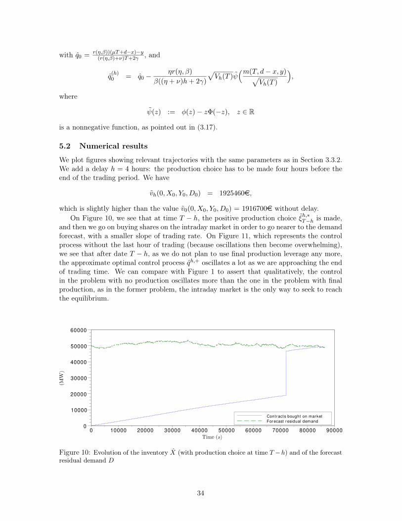
with q0 = r(η,β))(µT+d−x)−y(r(η,β)+ν)T+2γ , and

q(h)0 = q0 −

ηr(η, β)

β((η + ν)h+ 2γ)

√Vh(T )ψ

(m(T, d− x, y)√Vh(T )

),

where

ψ(z) := φ(z)− zΦ(−z), z ∈ R

is a nonnegative function, as pointed out in (3.17).

5.2 Numerical results

We plot figures showing relevant trajectories with the same parameters as in Section 3.3.2.We add a delay h = 4 hours: the production choice has to be made four hours before theend of the trading period. We have

vh(0, X0, Y0, D0) = 1925460e,

which is slightly higher than the value v0(0, X0, Y0, D0) = 1916700e without delay.On Figure 10, we see that at time T − h, the positive production choice ξh,∗T−h is made,

and then we go on buying shares on the intraday market in order to go nearer to the demandforecast, with a smaller slope of trading rate. On Figure 11, which represents the controlprocess without the last hour of trading (because oscillations then become overwhelming),we see that after date T − h, as we do not plan to use final production leverage any more,the approximate optimal control process qh,+ oscillates a lot as we are approaching the endof trading time. We can compare with Figure 1 to assert that qualitatively, the controlin the problem with no production oscillates more than the one in the problem with finalproduction, as in the former problem, the intraday market is the only way to seek to reachthe equilibrium.

Cont r acts bought on mar ket

For ecast r esidual demand

0

10000

20000

30000

40000

50000

60000

0 10000 20000 30000 40000 50000 60000 70000 80000 90000

Figure 10: Evolution of the inventory X (with production choice at time T −h) and of the forecastresidual demand D

34

Cont r ol

0.10

0.15

0.20

0.25

0.30

0.35

0 10000 20000 30000 40000 50000 60000 70000 80000 90000

Figure 11: Evolution of the trading rate control qh,+ without the last hour

A Appendix

A.1 Proof of Theorem 3.1

The Hamilton-Jacobi-Bellman (HJB) equation arising from the dynamic programming as-sociated to the stochastic control problem (3.4) is:∂v

∂t+ infq∈R

[q∂v

∂x+ νq

∂v

∂y+ µ

∂v

∂d+

1

2σ20∂2v

∂y2+

1

2σ2d∂2v

∂d2+ ρσ0σd

∂2v

∂y∂d+ q(y + γq)

]= 0,

v(T, x, y, d) = C(d− x) = 12r(η, β)(d− x)2.

The argmin in HJB is attained for

q(t, x, y, d) = − 1

2γ

[∂v∂x

+ ν∂v

∂y+ y],

and the HJB equation is rewritten as:∂v

∂t+ µ

∂v

∂d+

1

2σ20∂2v

∂y2+

1

2σ2d∂2v

∂d2+ ρσ0σd

∂2v

∂y∂d− 1

4γ

[∂v∂x

+ ν∂v

∂y+ y]

= 0,

v(T, x, y, d) = 12r(η, β)(d− x)2.

(A.1)

We look for a candidate solution to HJB in the form

w(t, x, y, d) = A(T − t)(d− x)2 +B(T − t)y2 + F (T − t)(d− x)y

+ G(T − t)(d− x) +H(T − t)y +K(T − t), (A.2)

for some deterministic functions A, B, F , G, H and K. Plugging the candidate function winto equation (A.1), we see that w is solution to the HJB equation iff the following systemof ordinary differential equations (ODEs) is satisfied by A, B, F , G, H and K:

A′ + 14γ (−2A+ νF )2 = 0

B′ + 14γ (2νB − F + 1)2 = 0

F ′ + 12γ (−2A+ νF )(2νB − F + 1) = 0

G′ − 2µA+ 12γ (−2A+ νF )(−G+ νH) = 0

H ′ − µF + 12γ (2νB − F + 1)(−G+ νH) = 0

K ′ − µG− (σ20B + σ2dA+ ρσ0σdF ) + 14γ (−G+ νH)2 = 0

35

with the initial conditions A(0) = 12r(η, β), B(0) = 0, F (0) = 0, G(0) = 0, H(0) = 0,

K(0) = 0. We first solve the Riccati system relative to the triple (A,B, F ), and obtain:A(t) =

r(η,β)( ν2t+γ)

(r(η,β)+ν)t+2γ ,

B(t) = −12

t(r(η,β)+ν)t+2γ , F (t) = r(η,β)t

(r(η,β)+ν)t+2γ .(A.3)

Then we solve the first-order linear system of ODE relative to the pair (G,H), which leadsto the explicit solution:

G(t) = 2µtA(t), and H(t) = −2r(η, β)µtB(t). (A.4)

Finally, we explicitly obtain K from the last equation:

K(t) = γσ20 + σ2dr

2(η, β)− 2ρσ0σdr(η, β)(r(η, β) + ν

)2 ln(

1 +(r(η, β) + ν)t

2γ

)+σ2dr(η, β)ν + 2ρσ0σdr(η, β)− σ20

2(r(η, β) + ν

) t +r(η, β)µ2t2(ν2 t+ γ)

(r(η, β) + ν)t+ 2γ. (A.5)

By construction, w in (A.2) with A, B, F , G, H and K explicitly given by (A.3)-(A.4)-(A.5), is a smooth solution with quadratic growth condition to the HJB equation (A.1).Moreover, the argmin in HJB equation for w is attained for

q(t, x, y, d) = − 1

2γ

[∂w∂x

+ ν∂w

∂y+ y]

=r(η, β)(µ(T − t) + d− x)− y

(r(η, β) + ν)(T − t) + 2γ=: q(T − t, d− x, y).

Notice that q is linear, and Lipschitz in x, y, d, uniformly in time t, and so given an initialstate (x, y, d) at time t, there exists a unique solution (Xt,x,y,d, Y t,x,y,d, Dt,d)t≤s≤T to (2.1)-(2.7)-(2.8) with the feedback control qs = q(T − s,Dt,d

s − Xt,x,y,ds , Y t,x,y,d

s ), which satisfies:E[supt≤s≤T |X

t,x,y,ds |2+|Y t,x,y,d

s |2+|Dt,ds |2] <∞. This implies in particular that E[

∫ Tt |qs|

2ds]<∞, hence q ∈ At. We now call on a classical verification theorem (see e.g. Theorem 3.5.2in [8]), which shows that w is indeed equal to the value function v, and q is an optimalcontrol. Finally, once the optimal trading rate q is determined, the optimal production isobtained from the optimization over ξ ∈ R of the terminal cost C(Dt,d

T − Xt,x,y,dT , ξ), hence

given by: ξT = ηη+β (Dt,d

T − Xt,x,y,dT ).

A.2 Proof of Theorem 4.1

The Hamilton-Jacobi-Bellman (HJB) integro-differential equation arising from the dynamicprogramming associated to the stochastic control problem v = v(λ) with jumps in the dy-namics of Y and D is:∂v(λ)

∂t+ infq∈R

[q∂v(λ)

∂x+ νq

∂v(λ)

∂y+ µ

∂v(λ)

∂d+

1

2σ20∂2v(λ)

∂y2+

1

2σ2d∂2v(λ)

∂d2+ ρσ0σd

∂2v(λ)

∂y∂d+ q(y + γq)

]+ λ

[p+v(λ)(t, x, y + π+, d+ δ+) + p−v(λ)(t, x, y + π−, d+ δ−)− v(λ)(t, x, y, d)

]= 0

v(λ)(T, x, y, d) = C(d− x) = 12r(η, β)(d− x)2.

36

Notice that with respect to the no jump case, there is in addition a linear integro-differentialterm in the HJB equation (which does not depend on the control), and the argmin is attainedas in the no jump case for

q(λ)(t, x, y, d) = − 1

2γ

[∂v(λ)∂x

+ ν∂v(λ)

∂y+ y].

The HJB equation is then rewritten as∂v(λ)

∂t+ µ

∂v(λ)

∂d+

1

2σ20∂2v(λ)

∂y2+

1

2σ2d∂2v(λ)

∂d2+ ρσ0σd

∂2v(λ)

∂y∂d− 1

4γ

[∂v(λ)∂x

+ ν∂v(λ)

∂y+ y]

+ λ[p+v(λ)(t, x, y + π+, d+ δ+) + p−v(λ)(t, x, y + π−, d+ δ−)− v(λ)(t, x, y, d)

]= 0

v(λ)(T, x, y, d) = 12r(η, β)(d− x)2.

(A.6)We look again for a candidate solution to (A.6) in the form

w(λ)(t, x, y, d) = Aλ(T − t)(d− x)2 +Bλ(T − t)y2 + Fλ(T − t)(d− x)y

+ Gλ(T − t)(d− x) +Hλ(T − t)y +Kλ(T − t), (A.7)

for some deterministic functions Aλ, Bλ, Fλ, Gλ, Hλ and Kλ. Plugging the candidatefunction w(λ) into equation (A.6), we see that w(λ) is solution to the HJB equation iff thefollowing system of ordinary differential equations (ODEs) is satisfied by Aλ, Bλ, Fλ, Gλ,Hλ and Kλ:

A′λ + 14γ (−2Aλ + νFλ)2 = 0

B′λ + 14γ (2νBλ − Fλ + 1)2 = 0

F ′λ + 12γ (−2Aλ + νFλ)(2νBλ − Fλ + 1) = 0

G′λ − 2µAλ + 12γ (−2Aλ + νFλ)(−Gλ + νHλ)− λ(2δAλ + πFλ) = 0

H ′λ − µFλ + 12γ (2νBλ − Fλ + 1)(−Gλ + νHλ)− λ(2πBλ + δFλ) = 0

K ′λ − µGλ − (σ20Bλ + σ2dAλ + ρσ0σdFλ) + 14γ (−Gλ + νHλ)2

−λ[(p+(δ+)2 + p−(δ−)2)Aλ + (p+(π+)2 + p−(π−)2)Bλ+(p+δ+π+ + p−δ−π−)Fλ + δGλ + πHλ] = 0

with the initial conditions Aλ(0) = 12r(η, β), Bλ(0) = 0, Fλ(0) = 0, Gλ(0) = 0, Hλ(0) = 0,

Kλ(0) = 0. We first solve the Riccati system relative to the triple (Aλ, Bλ, Fλ), which isthe same as in the no jump case, and therefore obtain: Aλ = A, Bλ = B, Fλ = F as in(A.3). Then we solve the first-order linear system of ODE relative to the pair (Gλ, Hλ),which involves the jump parameters λ, π and δ, and get:

Gλ(t) = G(t) +λ

2

r(η, β)t(πt+ 2δ(νt+ 2γ))

(r(η, β) + ν)t+ 2γ,

Hλ(t) = H(t)− λ

2

(π − 2r(η, β)δ)t2

(r(η, β) + ν)t+ 2γ,

37

where G and H are given from the no jump case (A.4). Finally, after some tedious butstraightforward calculations, we explicitly obtain Kλ from the last equation:

Kλ(t) = K(t) + λγp+(π+ − r(η, β)δ+)2 + p−(π− − r(η, β)δ−)2(

r(η, β) + ν)2 ln

(1 +

(r(η, β) + ν)t

2γ

)− λ

2

p+((π+)2 − r(η, β)δ+(2π+ + νδ+)) + p−((π−)2 − r(η, β)δ−(2π− + νδ−))

r(η, β) + νt

+λr(η, β)

2

2νµδ + λ((p+)2δ+(π+ + νδ+) + (p−)2δ−(π− + νδ−))

r(η, β) + νt2

+ λ2γr(η, β)r(η, β)δ2 + 2νp+p−δ+δ− − ((p+)2δ+π+ + (p−)2δ−π−)

(r(η, β) + ν)((r(η, β) + ν)t+ 2γ

) t2

+2λγr(η, β)2µδ

(r(η, β) + ν)((r(η, β) + ν)t+ 2γ

) t2 − λ2π2

48γt3

+λ2p+p−r(η, β)

2

2νδ+δ− + δ−π+ + δ+π−

(r(η, β) + ν)t+ 2γt3

+1

8

4r(η, β)µλπ − λ2π2

(r(η, β) + ν)t+ 2γt3,

with K in (A.5). The function w(λ) in (A.7) may thus be rewritten as the sum of w in(A.2) and another function of t, d − x and y, and is by construction a smooth solutionwith quadratic growth condition to the HJB equation (A.6). Moreover, the argmin in HJBequation for w(λ) is attained for

q(λ)(t, x, y, d) = − 1

2γ

[∂w(λ)

∂x+ ν

∂w(λ)

∂y+ y]

=r(η, β)(µ(T − t) + d− x)− y

(r(η, β) + ν)(T − t) + 2γ

+ λr(η, β)δ(T − t) + π

4γ (r(η, β) + ν)(T − t)2

(r(η, β) + ν)(T − t) + 2γ

=: q(λ)(T − t, d− x, y).

Again, notice that q(λ) is linear, and Lipschitz in x, y, d, uniformly in time t, and so given aninitial state (x, y, d) at time t, there exists a unique solution (Xt,x,y,d, Y t,x,y,d, Dt,d)t≤s≤T to(2.1)-(4.3)-(4.1) with the feedback control q(λ)s = q(λ)(T − s,Dt,d

s − Xt,x,y,ds , Y t,x,y,d

s ), whichsatisfies: E[supt≤s≤T |X

t,x,y,ds |2+ |Y t,x,y,d

s |2+ |Dt,ds |2] <∞, see e.g. Theorem 1.19 in [7]. This

implies that E[∫ Tt |q

(λ)s |2ds] < ∞, hence q(λ) ∈ At. We now call on a classical verification

theorem for stochastic control of jump-diffusion processes (see e.g. Theorem 3.1 in [7]),which shows that w(λ) is indeed equal to the value function v(λ), and q(λ) is an optimalcontrol. Finally, once the optimal trading rate q(λ) is determined, the optimal production isobtained from the optimization over ξ ∈ R of the terminal cost C(Dt,d

T − Xt,x,y,dT , ξ), hence

given by: ξ(λ)T = ηη+β (Dt,d

T − Xt,x,y,dT ).

38

References[1] R. Aïd. Electricity Derivatives. Springer Briefs in Quantitative Finance. Springer-Verlag, 2015.

[2] R. Almgren and N. Chriss. Optimal execution of portfolio transactions. Journal of Risk, 3:5–39,2000.

[3] A. Bensoussan, P. Bertrand and A. Brouste. A generalized model approach to seasonal aspectsof wind speed modeling. Journal of Applied Statistics, 41(8):1694–1707, 2014.

[4] E. Garnier and R. Madlener. Balancing forecast errors in continuous-trade intraday markets.FCN WP 2/2014, RWTH Aachen University School of Business and Economics, 2014.

[5] G. Giebel, G. Kariniotakis, R. Brownsword, M. Denhard and C. Draxl. The state-of-the-art inshort-term prediction of wind power. A literature overview. 2nd Edition. In Deliverable ReportD1.2 of the Anemos Project (ENK5-CT-2002-00665), 2011.

[6] A. Henriot. Market design with centralised wind power management: handling low-predictabilityin intraday markets. The Energy Journal, 35(1):99–117, 2014.

[7] B. Øksendal and A. Sulem. Applied stochastic control of jump diffusions. Universitext. Springer,Berlin, second edition, 2007.

[8] H. Pham. Continuous-time stochastic control and optimization with financial applications, Vol.61 of Stochastic Modelling and Applied Probability. Springer-Verlag, Berlin, 2009.

[9] A. Schied and A. Slynko. Some mathematical aspects of market impact modeling. In Surveysin stochastic processes, EMS Ser. Congr. Rep., pages 153–179. Eur. Math. Soc., Zürich, 2011.

[10] D. Williams. Probability with martingales. Cambridge mathematical text, 1991.

39