An Open Source Discussion Group Recommendation … · III The Designated Project Committee Approves...

I

An Open Source Discussion Group Recommendation System

A Project Presented to

The Faculty of the Department of Computer Science

San Jose State University

In Partial Fulfillment

of the Requirements for the Degree

Master of Science

by

Sarika Padmashali

May 2017

II

© 2017

Sarika Padmashali

ALL RIGHTS RESERVED

III

The Designated Project Committee Approves the Master’s Project Titled


by

Sarika Padmashali

APPROVED FOR THE DEPARTMENT OF COMPUTER SCIENCE

SAN JOSE STATE UNIVERSITY

May 2016

Dr. Chris Pollett, Department of Computer Science

Dr. Katerina Potika, Department of Computer Science

Dr. Leonard Wesley, Department of Computer Science

APPROVED FOR THE UNIVERSITY

Associate Dean Office of Graduate Studies and Research

IV

ABSTRACT


by Sarika Padmashali

A recommendation system analyzes user behavior on a website to make suggestions

about what a user should do in the future on the website. It basically tries to predict the “rating”

or “preference” a user would have for an action. Yioop is an open source search engine, wiki

system, and user discussion group system managed by Dr. Christopher Pollett at SJSU. In this

project, we have developed a recommendation system for Yioop where users are given

suggestions about the threads and groups they could join based on their user history. We have

used collaborative filtering techniques to make recommendations and have tried to leverage user

and the thread or group biases to make predictions. We have also made use of term frequency-

inverse document frequency to improve our recommendations. We have integrated the

recommendation system with Yioop and tested its effectiveness by asking nearly 100 users and

found that it recommended exciting and interesting threads and groups 90 percent of the time.

V

ACKNOWLEDGEMENT

I would like to dedicate this project to my parents and brother who have showered their

unconditional love and support throughout my master’s program. I would like to give my deepest

gratitude to Dr. Christopher Pollett for being so patient with me, bolstering my ideas when my

mind was in doubt, coming up with suggestions that would help me improve my project and for

being so cool throughout the project which spanned for a year. I would also like to extend my

gratitude to my committee members, Dr. Katerina Potika and Dr. Leonard Wesley for their

suggestions and time.

I would like to thank my mentor Mr. James Casaletto for his enduring support on all

fronts – professionally, morally and academically. I would also like to thank all my friends

without whom this would not have been possible. Thank you Nirali and Shikha for everything.

VI

TABLE OF CONTENTS

1. INTRODUCTION...........................................................................................1

2. BACKGROUND.............................................................................................3

2.1CollaborativeFiltering–LatentMatrixFactorization.................................4

2.2AboutYioopDiscussionGroup...................................................................5

3. COLLABORATIVEFILTERING-BASELINEPREDICTOR.....................................7

4. TERMFREQUENCY-INVERSEDOCUMENTFREQUENCY(TF-IDF).................9

4.1Informationretrievalprobleminsearchengines.......................................9

4.2OverviewofTF-IDF..................................................................................10

4.2.1TermFrequency(TF)...............................................................................10

4.2.2InverseDocumentFrequency(IDF)........................................................15

4.2.3WeightsTF*IDF.......................................................................................17

4.2.4CosineSimilarity.....................................................................................18

5.ARECOMMENDATIONSYSTEMFORYIOOP...................................................19

5.1Recommendingtrendingthreadstousers...............................................19

5.1.1Calculatingtheuseranditembiases......................................................20

5.2RecommendingthreadstousersbyincorporatingtheTF–IDFmeasure.22

5.2.1Calculatingthetermfrequencyforeachthread....................................23

5.2.2Calculatingthetermfrequencyforeachuser........................................24

5.2.3CalculatingtheIDFforthreads...............................................................25

5.2.5CalculatingtheweightsTF*IDF...............................................................26

5.2.6Cosinesimilarity.....................................................................................27

5.3Recommendinggroups............................................................................27

VII

5.4AdvantagesoftheTF–IDFmethodforRecommendingthreads/groups..28

6. RUNNINGTHERECOMMENDATIONJOB.....................................................29

6.1OfflineJob–ComputationPart................................................................29

6.2OnlineRecommendations–RenderingPart.............................................30

6.3IncrementalJob.......................................................................................30

7.USERINTERFACE...........................................................................................32

8.EXPERIMENTSANDTESTING.........................................................................35

9.CONCLUSIONSANDFUTUREWORK..............................................................37

9.1MultimodalRecommendations...............................................................37

10.BIBLIOGRAPHY...........................................................................................40

VIII

LIST OF FIGURES

Figure 1 Collaborative Filtering Technique .............................................................. 3

Figure 2 Total Average Rating Based on The Sample Yioop Dataset. .................. 19

Figure 3 User Bias Based on The Sample Yioop Dataset. ..................................... 20

Figure 4 Thread Bias Based on The Sample Yioop Dataset. .................................. 21

Figure 5 Predicted User Rating Based on Sample Yioop Dataset. ......................... 21

Figure 6 Shows the Title and Description Entries in the GROUP_ITEM Table. ... 22

Figure 7 Shows the Bag of Words Built from the Title and Description attributes.

.......................................................................................................................... 23

Figure 8 Term Frequency of Each Thread in Sample Yioop Dataset. .................... 24

Figure 9 Term Frequency of Each User in Sample Yioop Dataset. ........................ 25

Figure 10 IDF Table on Sample Yioop Dataset. ..................................................... 26

Figure 11 Item Word Weights Table on Sample Yioop Dataset. ........................... 26

Figure 12 User Word Weights Table on Sample Yioop Dataset. ........................... 27

Figure 13 Threads Recommended to a user on Sample Yioop Dataset. ................. 27

Figure 14 Groups Recommended to a User on Sample Yioop Dataset. ................. 28

Figure 15 Threads which the user Bob2 is a part of in Yioop. ............................... 33

Figure 16 Threads recommended to a user Bob2. .................................................. 33

Figure 17 Groups recommended to a user Bob2. ................................................... 34

Figure 18 Trending groups recommended to a user Bob2. ..................................... 34

Figure 19 Recommendations given to a user in Yioop. .......................................... 34

Figure 20 Unit Testing Code to Check the Word Count. ....................................... 35

Figure 21 Screenshot of Test Results. ..................................................................... 36

Figure 22 Multimodal Recommendation System. .................................................. 39

IX

LIST OF TABLES

Table 1 Term Frequency for Document 1 ............................................................... 12


Table 3 Term Frequency for Document 2 continued .............................................. 12


Table 5 Logarithmic Term Frequency for Document 1 .......................................... 14


Table 7 Logarithmic Term Frequency for Document 2 continued ......................... 14


Table 9 Inverse Document Frequency for all words in the Documents ................. 16

Table 10 Weights for the Query Terms in the Documents ..................................... 17

Table 11 Weights for the Query Terms for the user ............................................... 18

1

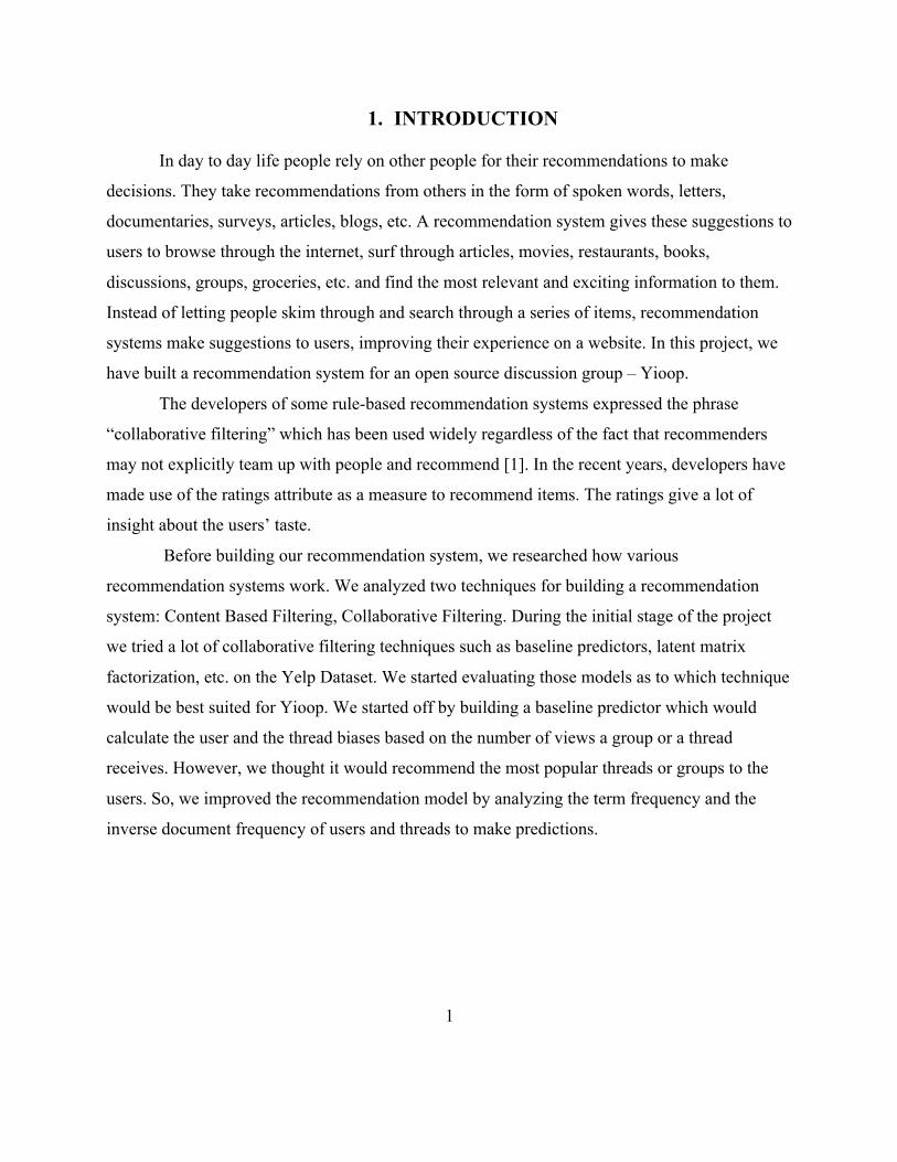
1. INTRODUCTION

In day to day life people rely on other people for their recommendations to make

decisions. They take recommendations from others in the form of spoken words, letters,

documentaries, surveys, articles, blogs, etc. A recommendation system gives these suggestions to

users to browse through the internet, surf through articles, movies, restaurants, books,

discussions, groups, groceries, etc. and find the most relevant and exciting information to them.

Instead of letting people skim through and search through a series of items, recommendation

systems make suggestions to users, improving their experience on a website. In this project, we

have built a recommendation system for an open source discussion group – Yioop.

The developers of some rule-based recommendation systems expressed the phrase

“collaborative filtering” which has been used widely regardless of the fact that recommenders

may not explicitly team up with people and recommend [1]. In the recent years, developers have

made use of the ratings attribute as a measure to recommend items. The ratings give a lot of

insight about the users’ taste.

Before building our recommendation system, we researched how various

recommendation systems work. We analyzed two techniques for building a recommendation

system: Content Based Filtering, Collaborative Filtering. During the initial stage of the project

we tried a lot of collaborative filtering techniques such as baseline predictors, latent matrix

factorization, etc. on the Yelp Dataset. We started evaluating those models as to which technique

would be best suited for Yioop. We started off by building a baseline predictor which would

calculate the user and the thread biases based on the number of views a group or a thread

receives. However, we thought it would recommend the most popular threads or groups to the

users. So, we improved the recommendation model by analyzing the term frequency and the

inverse document frequency of users and threads to make predictions.

2

This report is organized as follows: Chapter 2 gives a background of collaborative

filtering techniques. Chapter 3 discusses collaborative filtering – baseline predictor in detail.

Chapter 4 contains detailed explanations of the Collaborative Filtering Method, Term Frequency

– Inverse Document Frequency and Cosine Similarity. Chapter 5 discusses how the

recommendation system is built in Yioop. It gives more details about the integration with the

media jobs in Yioop. Chapter 6 gives details about how the job is run in batch mode and running

mode. Chapter 7 consists some screenshots which gives information about the user interface.

Chapter 8 discusses the unit testing to ensure the proper working of Yioop with the

recommendation system and the various experiments performed to test its effectiveness. Chapter

9 concludes the project and discusses about the future work on this project.

3

2. BACKGROUND

In this chapter, we define the term collaborative filtering, explain the latent matrix

factorization technique in detail and give some background about Yioop. Collaborative filtering

techniques are based on the simple idea that users who rate items similarly are likely to rate other

items similarly. Sometimes ratings are unavailable in such cases users who have similar behavior

such as watching, buying, listening, etc., can be thought of having the same taste.

Figure 1 Collaborative Filtering Technique

Figure 1 gives an illustration of the basic working of collaborative filtering. Chris

purchases strawberries, oranges and mangoes, Sarika buys mangoes and watermelons, while Joe

buys watermelon. What else would we suggest Joe? We see that the shopping pattern of Sarika

and Joe are similar hence we suggest Joe to buy mangoes.

4

2.1 Collaborative Filtering – Latent Matrix Factorization

Recommendation systems can be built by a variety of algorithms. User based and item

based recommendations are very intuitive and simple to implement, matrix factorization

techniques are sophisticated algorithms which helps us to discover latent features between the

interactions of users and items. Matrix factorization is a simple tool which helps us to discover

the information hidden under data. As the name implies matrix factorization intends to factorize

the matrix i.e., find the two or more matrices which when multiplied will give us back the

original matrix. Matrix factorization helps in finding the association between two different kind

of entities. Hence, it finds an application for predicting a user’s rating.

We researched about this technique, however, could not use this technique to build our

recommendation model as it required the rating metric which we lacked in our system. Also, the

technique is computationally intensive.

In a recommendation system, for any website, there are a bunch of users and a bunch of

items. Let us consider a matrix where each user has rated some items in the system, and we

would like to predict the missing cells in the matrix i.e., trying to predict the rating of the items

which the user has not rated yet in such a way that the new predictions are consistent with the

existing ratings i.e., original matrix.

The basic idea behind latent matrix factorization is the fact that if two or more users are

giving high rating to an item, it is because they like some latent (hidden) feature behind that

item. In the case of movies, these hidden features might be the genre or the actor/actresses of the

movie. For a restaurant, it might be the cuisine, or the ambience or any such other feature.

Hence, if we can somehow capture these hidden features then we can map the users with the

items as there is a common feature associated with both the users and the items (for example, the

hidden feature actor is a common feature which maps the users with movies). Also, the number

of features would be very less as compared to the number of items or users, otherwise, there is no

need to have a recommendation system in the first place.

5

Let us take a very quick example and understand the mathematics behind matrix

factorization. Now if we have a matrix 𝑅 which will be a matrix of users and item ids. Suppose

we have𝑚users and n items, we now want to find 𝑘 latent features. We must find the two

matrices 𝑃 and 𝑄 such that their product is approximately 𝑅. Thus, matrix 𝑃 would be a m by k

matrix and matrix 𝑄 would be a k by n matrix.

𝑅 ≈ 𝑃.𝑄) = 𝑅

Now from the above equations we can say that each row of 𝑃 is an association between

features and users. Similarly, each row in 𝑄 is an association between features and items. Hence

now to predict how a user rates an item we just take the dot product. For our research, we have

used the gradient descent method to find the matrices 𝑃and 𝑄. Gradient descent initializes the

matrix 𝑃 and 𝑄 with some numbers and tries to find the variance between the obtained matrix

and original matrix 𝑅 and tries to minimize the error. We minimize the error by finding the

direction in which we need to modify the current values. We find the gradient at the current

values by differentiating with respect to both the variables. Once we find the gradient we can

multiply it with a constant α and add it to the current values. α determines the rate at which we

want the error to approach the minimum.

2.2 About Yioop Discussion Group

Yioop is an open source search engine and discussion group software [6]. Yioop is

a GPLv3, open source, PHP search engine [6]. Yioop provides many features of large search

portals such as search results, media services, social groups, blogs and wikis [6]. Yioop allows

users to create discussion groups and start a new thread on those groups where they can discuss

with other Yioop users. We have developed a recommendation engine which suggests users with

threads or groups might be of interest to them based on the threads or groups a user has viewed

in the past. We also suggest the trending threads or groups to users based on their number of

views.

6

Our recommendation system suggests the users with two items:

1. Threads

2. Groups

We have incorporated two versions of baseline predictors to improve user experience and to

give better results.

1. Suggest trending and popular threads to users using the classic baseline predictor

model.

2. Suggest the threads or groups to users based on the words they have liked to view in

the past.

7

3. COLLABORATIVE FILTERING - BASELINE PREDICTOR

The Netflix Prize was an open competition to build a recommendation model using

collaborative filtering to predict user ratings for movies, based on the previous rating given by

the users. The participants were not given any information about the users or the movies. We

have used parts of the contribution to the “Bell- Kor’s Pragmatic Chaos” final solution, which

won the Netflix Grand Prize to recommend threads or groups to users [3].

Collaborative filtering model try to capture the interaction between the users and the

items that produce ratings differently [3]. For example, two users 𝐴 and 𝐵 rate a movie Notebook

4 and 1 respectively based on their taste. There is something about the movie which the user 𝐵

did not like and hence rated it poorly. Hence, most of the ratings are due to the associations

between the users and the items. There are some biases between the users and the items. For

example, some users have a tendency of rating generously whereas some users have a tendency

of rating poorly. Similarly, some items get higher ratings than other items. The baseline predictor

tries to leverage these biases and encapsulate those hidden effects which do not involve any user-

item interaction with baseline predictors [3].

Let 𝑟 denote the total average rating. A baseline predictor for an unknown rating 𝑟.,0 is denoted

by the 𝑏.,0 and accounts for the user and item effects.

𝑏.0 = 𝑟 +𝑏. + 𝑏0

The metrics 𝑏.and 𝑏0represent how far the user is deviated from the average rating 𝑟.

Suppose we want to predict what user "Sarika" would rate the restaurant "In-n-Out Burger" and

the overall average rating = 3.7, the users and the restaurants bias comes out to be 1.7 and - 1.2

respectively then the predicted rating would be 3.7 + 1.7 - 1.2 = 4.2.

Let us separate out the individual components of the biases. Let us first calculate the user

biases followed by the item biases. Now for each user 𝑖 in the corpus we first calculate the user

bias for 𝑖 by summing all the ratings which the user has rated and divide it by the number of

items rated by the user. We now subtract this computed measure from the total average rating

which shows us how much a user is deviating from the average rating.

8

For example, if a user A has rated three movies on 5 as 3 ,2, 1 respectively; the overall

average rating for all the users is 3.5; then the bias computed for that user would be – 1.5. This

clearly states that the user A has a systematic tendency of rating movies, poorly i.e. below the

average rating. We can learn a lot by finding these biases, it helps us understand the users pattern

of ratings and hence will help us give better predictions of the kind of the items people would

like.

Similarly, for the items, there are certain items which are very popular and are rated the

highly whereas some items are rated poorly. This metric shows a lot about the quality of items. If

an item is rated high by majority that implies that the item is popular among the masses and is

liked by item. Now when we predict the rating a user might give to an item which is the sum of

the user bias, the item bias and the overall average rating. We have considered the kind of rating

a user gives, the quality of the items and the overall average rating. This way we get an insight

about the users taste towards an item.

One of the challenges while building a baseline predictor for a dataset is the absence of

ratings. The matrix of users and their ratings for items is sparse. Most of the time users do not

rate; few users rate a lot of items while some rate very few items. The baseline predictors help in

reducing these biases as the computation sees how a user rates an item. Sometimes there are no

ratings at all. In our project, the users have not voted or given ratings to any threads or groups.

So, we decided to work around this and make use of the user’s history so make predictions –

what the user is watching and likes to watch. These challenges are discussed in depth later in

chapter 5.

9

4. TERM FREQUENCY - INVERSE DOCUMENT FREQUENCY (TF - IDF)

We have made use of the Term Frequency and the Inverse Document Frequency

technique and tweaked it according to our use case, so that we could build a recommendation

system for Yioop. In this chapter, we have discussed about the term frequency and the inverse

document frequent in detail.

Usually whenever a user performs a search query, if a document contains the terms in the

query then we score that document as being relevant. However, the number of occurrences of a

word in a document is not taken into consideration while weighing the relevance of a document.

The term frequency and the inverse document frequency tries to weigh the documents in a way

that the frequency of the terms is taken into consideration while weighing its relevance. TF-IDF

scores each word in a document through a proportion of the percent of documents the word

appears in to the frequency of the word in a document [2]. Words with a high TF-IDF value in a

document implies a strong relationship of the word with the document. Thus, if a user query

contains this word it might be an interesting document to the user.

4.1 Information retrieval problem in search engines.

The task of retrieving data from a user’s behavior has become so common and necessary

in the recent years. From building search engines to recommendation systems, retrieving

information about a user’s behavior has been an important aspect in most of the applications.

Information retrieval can be described as searching a collection of data from text

documents, databases, log searches etc. and gaining insights about that data. The problem can be

described as searching the corpus for relevant documents and finding the documents which are

most relevant to the user’s query.

There are many approaches available to retrieve information from, in the search engines.

There are many statistical methods which are efficient in solving the problem such as in 1999

10

Berger & Lafferty proposed a probabilistic model incorporating the user’s frame of mind while

the user entered a query and enhancing the approximations to make better suggestions [2].

The idea behind this is that the user has a mindset 𝐾 and his query consists of words 𝑞.

By applying transformation of 𝐾 into 𝑞 we can return the relevant documents and by applying

Bayes law they returned relevant documents [2].

There is some vector based methods for performing query retrieval such as the one

proposed by Berry, Dumais & Obrien in 1994[2] which made use of Latent Semantic Indexing

(LSI). The algorithm builds a reduced dimensional vector space which represents the n-

dimensional representation of a set of documents. Whenever a user enters a query, the numerical

value is calculated for the query and cosine distance of that query is measured with the entire

corpus of documents. The set of documents which has the least distances is returned to the user.

4.2 Overview of TF-IDF

TF-IDF makes use of the measure of the count of the words to return relevant documents.

Based on terms the users query consists of Term frequency - Inverse Document Frequency aims

at finding the documents which are most relevant to the user’s query. To solve this problem, we

calculate two metrics – term frequency and the inverse document frequency. Let us make use of

an example to describe this problem. We will first describe the problem followed by the

mathematical background of the algorithm and examine the behavior of various variables in the

following sections. Let us suppose we have a set of documents 𝐷:𝑑9,𝑑:, 𝑑;, … , 𝑑= and a user

query 𝑞 = 𝑤9,𝑤:, 𝑤; for a set of words 𝑤0. We want to return the subset of D documents which

are the most relevant documents in the corpus based on the user’s query.

4.2.1 Term Frequency (TF)

The term frequency of a word in a document is the number of times a word appears in a

document. As an example, with three documents, try to understand the mathematics behind the

term frequency calculation.

11

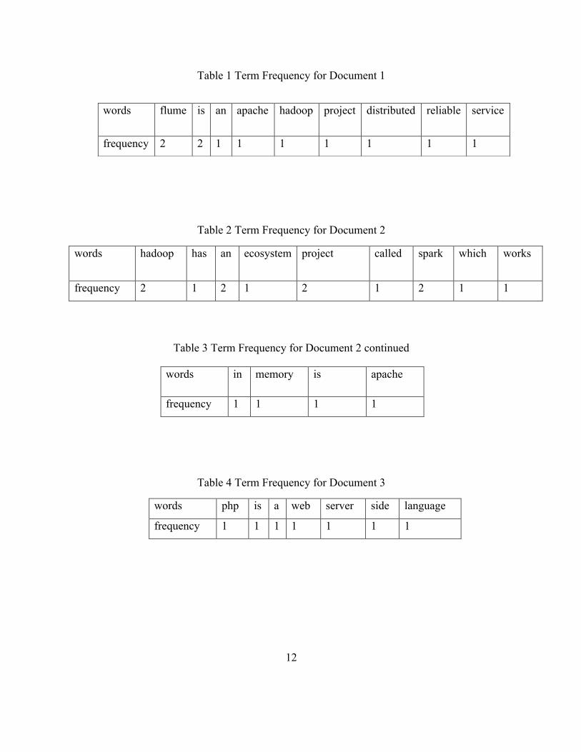
Document 1: Flume is an Apache Hadoop project. Flume is a distributed, reliable service.

Document 2: Hadoop has an ecosystem project called Spark which works in memory.

Spark is an Apache Hadoop project

Document 3: PHP is a good web server side programming language

Now let us assume that a user has entered a query q: Hadoop project. Usually web users

type a free text query i.e., they do not make use of a specific language or operators rather just use

words to make up the query expression. There is no proper structure which every user follows

for querying.

Term frequency measures the frequency of a word in a document. The table 1, table 2,

table 3 below shows the TF for the documents 1, 2 and 3 respectively.

12

Table 1 Term Frequency for Document 1


words hadoop has an ecosystem project called spark which works

frequency 2 1 2 1 2 1 2 1 1

Table 3 Term Frequency for Document 2 continued


words php is a web server side language

frequency 1 1 1 1 1 1 1

words flume is an apache hadoop project distributed reliable service

frequency 2 2 1 1 1 1 1 1 1

words in memory is apache

frequency 1 1 1 1

13

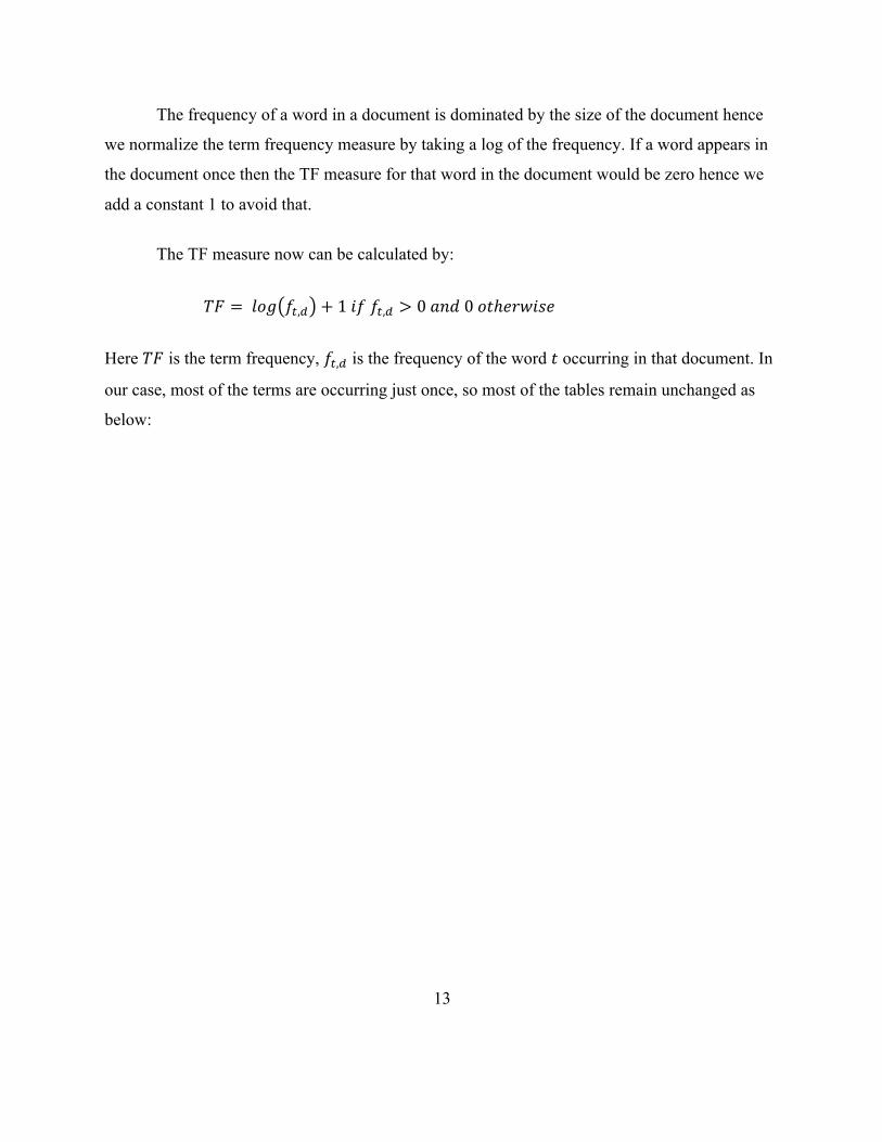
The frequency of a word in a document is dominated by the size of the document hence

we normalize the term frequency measure by taking a log of the frequency. If a word appears in

the document once then the TF measure for that word in the document would be zero hence we

add a constant 1 to avoid that.

The TF measure now can be calculated by:

𝑇𝐹 = 𝑙𝑜𝑔 𝑓E,F + 1𝑖𝑓𝑓E,F > 0𝑎𝑛𝑑0𝑜𝑡ℎ𝑒𝑟𝑤𝑖𝑠𝑒

Here 𝑇𝐹 is the term frequency, 𝑓E,F is the frequency of the word 𝑡 occurring in that document. In

our case, most of the terms are occurring just once, so most of the tables remain unchanged as

below:

14

Table 5 Logarithmic Term Frequency for Document 1


words hadoop has an ecosystem project called spark which works

frequency 0.4 1 0.4 1 0.4 1 0.4 1 1

Table 7 Logarithmic Term Frequency for Document 2 continued


words php is a web server side language

frequency 1 1 1 1 1 1 1

words flume is an apache hadoop project distributed reliable service

frequency 0.4 0.4 1 1 1 1 1 1 1

words in memory is apache

frequency 1 1 1 1

15

4.2.2 Inverse Document Frequency (IDF)

While calculating the term frequency we are considering that all the words are equally

important in a document. However, it does not take into consideration the effect of a few words

which occur in most of the documents. For examples, words like as, in, the etc., occur in almost

all the documents. Also, there are a few less frequently occurring words which occur only in a

few documents. So, the logarithm helps us to solve this problem.

Let us see the mathematics behind the calculation of IDF.

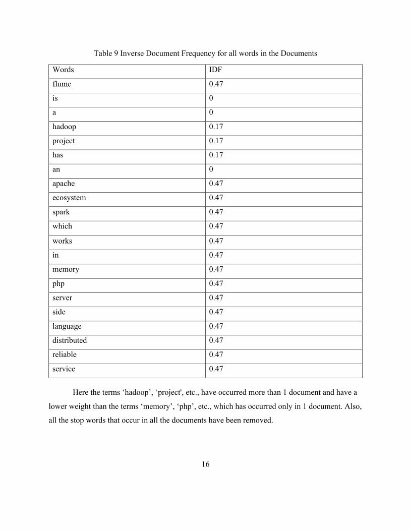
𝐼𝐷𝐹 𝑡 = log𝑁𝑁E

where ‘N’ is the total number of documents in the corpus and 𝑁E is the number of documents

containing the term 𝑡.

Let us compute the IDF for the word ‘hadoop’.

The total number of documents for our example is, 𝑁 = 3.

The number of documents which contains the term ‘hadoop’ is, 𝑁E = 2

𝐼𝐷𝐹 ℎ𝑎𝑑𝑜𝑜𝑝 = log32 = 0.17

Similarly, for all the words we calculate the IDF and we build the Table 9.

16

Table 9 Inverse Document Frequency for all words in the Documents

Words IDF

flume 0.47

is 0

a 0

hadoop 0.17

project 0.17

has 0.17

an 0

apache 0.47

ecosystem 0.47

spark 0.47

which 0.47

works 0.47

in 0.47

memory 0.47

php 0.47

server 0.47

side 0.47

language 0.47

distributed 0.47

reliable 0.47

service 0.47

Here the terms ‘hadoop’, ‘project', etc., have occurred more than 1 document and have a

lower weight than the terms ‘memory’, ‘php’, etc., which has occurred only in 1 document. Also,

all the stop words that occur in all the documents have been removed.

17

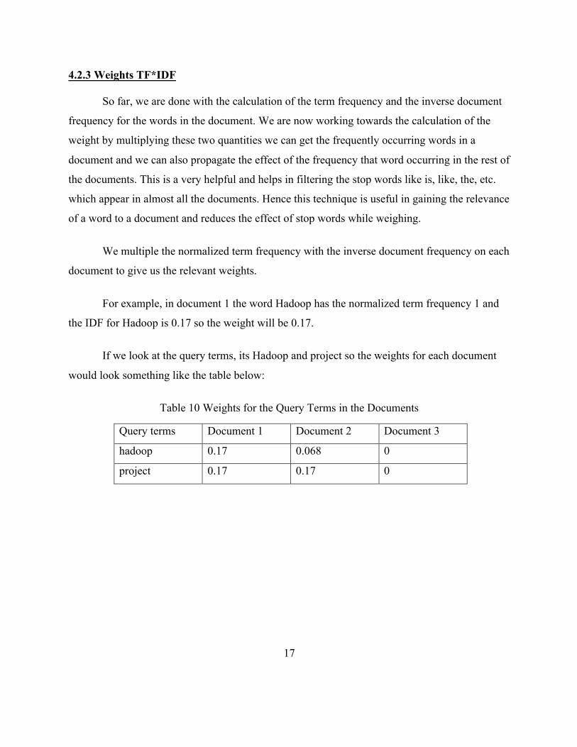
4.2.3 Weights TF*IDF

So far, we are done with the calculation of the term frequency and the inverse document

frequency for the words in the document. We are now working towards the calculation of the

weight by multiplying these two quantities we can get the frequently occurring words in a

document and we can also propagate the effect of the frequency that word occurring in the rest of

the documents. This is a very helpful and helps in filtering the stop words like is, like, the, etc.

which appear in almost all the documents. Hence this technique is useful in gaining the relevance

of a word to a document and reduces the effect of stop words while weighing.

We multiple the normalized term frequency with the inverse document frequency on each

document to give us the relevant weights.

For example, in document 1 the word Hadoop has the normalized term frequency 1 and

the IDF for Hadoop is 0.17 so the weight will be 0.17.

If we look at the query terms, its Hadoop and project so the weights for each document

would look something like the table below:

Table 10 Weights for the Query Terms in the Documents

Query terms Document 1 Document 2 Document 3

hadoop 0.17 0.068 0

project 0.17 0.17 0

18

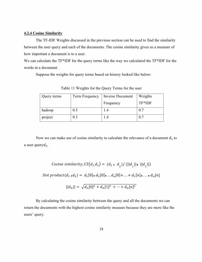
4.2.4 Cosine Similarity

The TF-IDF Weights discussed in the previous section can be used to find the similarity

between the user query and each of the documents. The cosine similarity gives us a measure of

how important a document is to a user.

We can calculate the TF*IDF for the query terms like the way we calculated the TF*IDF for the

words in a document.

Suppose the weights for query terms based on history looked like below:

Table 11 Weights for the Query Terms for the user

Query terms Term Frequency Inverse Document

Frequency

Weights

TF*IDF

hadoop 0.5 1.4 0.7

project 0.5 1.4 0.7

Now we can make use of cosine similarity to calculate the relevance of a document 𝑑9to

a user query𝑑:.

𝐶𝑜𝑠𝑖𝑛𝑒𝑠𝑖𝑚𝑖𝑙𝑎𝑟𝑖𝑡𝑦, 𝐶𝑆 𝑑9,𝑑: = (𝑑9.𝑑2)/(||𝑑1||. ||𝑑2||) 𝐷𝑜𝑡𝑝𝑟𝑜𝑑𝑢𝑐𝑡(𝑑9.𝑑:) = 𝑑9 0 . 𝑑: 0 .…𝑑= 0 +. . . +𝑑9 𝑛 . . . . . 𝑑=[𝑛]

||𝑑=|| = 𝑑=[0]: + 𝑑=[1]: + ⋯+𝑑=[𝑛]:

By calculating the cosine similarity between the query and all the documents we can

return the documents with the highest cosine similarity measure because they are more like the

users’ query.

19

5. A RECOMMENDATION SYSTEM FOR YIOOP

5.1 Recommending trending threads to users

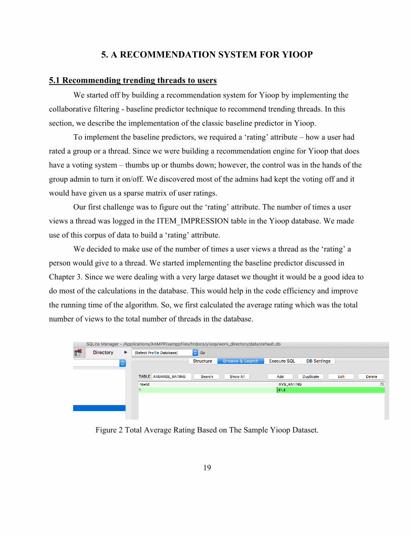
We started off by building a recommendation system for Yioop by implementing the

collaborative filtering - baseline predictor technique to recommend trending threads. In this

section, we describe the implementation of the classic baseline predictor in Yioop.

To implement the baseline predictors, we required a ‘rating’ attribute – how a user had

rated a group or a thread. Since we were building a recommendation engine for Yioop that does

have a voting system – thumbs up or thumbs down; however, the control was in the hands of the

group admin to turn it on/off. We discovered most of the admins had kept the voting off and it

would have given us a sparse matrix of user ratings.

Our first challenge was to figure out the ‘rating’ attribute. The number of times a user

views a thread was logged in the ITEM_IMPRESSION table in the Yioop database. We made

use of this corpus of data to build a ‘rating’ attribute.

We decided to make use of the number of times a user views a thread as the ‘rating’ a

person would give to a thread. We started implementing the baseline predictor discussed in

Chapter 3. Since we were dealing with a very large dataset we thought it would be a good idea to

do most of the calculations in the database. This would help in the code efficiency and improve

the running time of the algorithm. So, we first calculated the average rating which was the total

number of views to the total number of threads in the database.

Figure 2 Total Average Rating Based on The Sample Yioop Dataset.

20

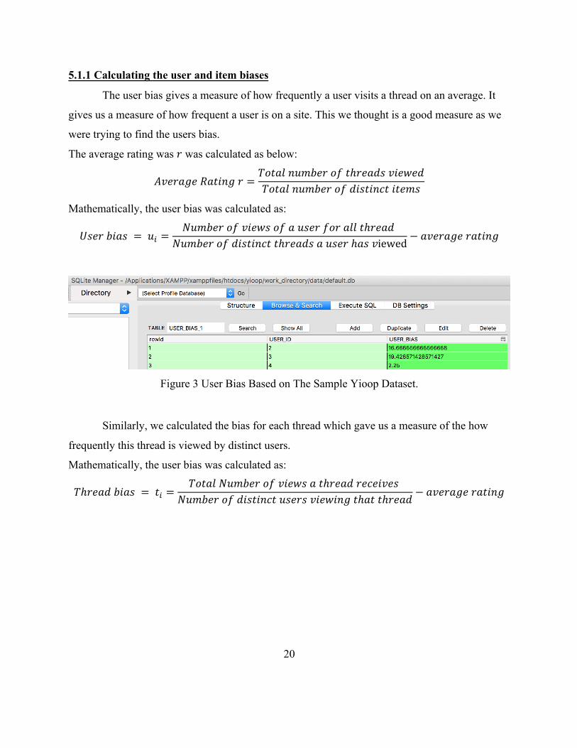
5.1.1 Calculating the user and item biases

The user bias gives a measure of how frequently a user visits a thread on an average. It

gives us a measure of how frequent a user is on a site. This we thought is a good measure as we

were trying to find the users bias.

The average rating was 𝑟 was calculated as below:

𝐴𝑣𝑒𝑟𝑎𝑔𝑒𝑅𝑎𝑡𝑖𝑛𝑔𝑟 =𝑇𝑜𝑡𝑎𝑙𝑛𝑢𝑚𝑏𝑒𝑟𝑜𝑓𝑡ℎ𝑟𝑒𝑎𝑑𝑠𝑣𝑖𝑒𝑤𝑒𝑑𝑇𝑜𝑡𝑎𝑙𝑛𝑢𝑚𝑏𝑒𝑟𝑜𝑓𝑑𝑖𝑠𝑡𝑖𝑛𝑐𝑡𝑖𝑡𝑒𝑚𝑠

Mathematically, the user bias was calculated as:

𝑈𝑠𝑒𝑟𝑏𝑖𝑎𝑠 = 𝑢0 =𝑁𝑢𝑚𝑏𝑒𝑟𝑜𝑓𝑣𝑖𝑒𝑤𝑠𝑜𝑓𝑎𝑢𝑠𝑒𝑟𝑓𝑜𝑟𝑎𝑙𝑙𝑡ℎ𝑟𝑒𝑎𝑑

𝑁𝑢𝑚𝑏𝑒𝑟𝑜𝑓𝑑𝑖𝑠𝑡𝑖𝑛𝑐𝑡𝑡ℎ𝑟𝑒𝑎𝑑𝑠𝑎𝑢𝑠𝑒𝑟ℎ𝑎𝑠𝑣iewed − 𝑎𝑣𝑒𝑟𝑎𝑔𝑒𝑟𝑎𝑡𝑖𝑛𝑔

Figure 3 User Bias Based on The Sample Yioop Dataset.

Similarly, we calculated the bias for each thread which gave us a measure of the how

frequently this thread is viewed by distinct users.

Mathematically, the user bias was calculated as:

𝑇ℎ𝑟𝑒𝑎𝑑𝑏𝑖𝑎𝑠 = 𝑡0 =𝑇𝑜𝑡𝑎𝑙𝑁𝑢𝑚𝑏𝑒𝑟𝑜𝑓𝑣𝑖𝑒𝑤𝑠𝑎𝑡ℎ𝑟𝑒𝑎𝑑𝑟𝑒𝑐𝑒𝑖𝑣𝑒𝑠

𝑁𝑢𝑚𝑏𝑒𝑟𝑜𝑓𝑑𝑖𝑠𝑡𝑖𝑛𝑐𝑡𝑢𝑠𝑒𝑟𝑠𝑣𝑖𝑒𝑤𝑖𝑛𝑔𝑡ℎ𝑎𝑡𝑡ℎ𝑟𝑒𝑎𝑑 − 𝑎𝑣𝑒𝑟𝑎𝑔𝑒𝑟𝑎𝑡𝑖𝑛𝑔

21

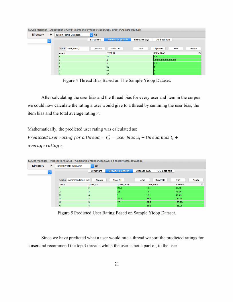
Figure 4 Thread Bias Based on The Sample Yioop Dataset.

After calculating the user bias and the thread bias for every user and item in the corpus

we could now calculate the rating a user would give to a thread by summing the user bias, the

item bias and the total average rating 𝑟.

Mathematically, the predicted user rating was calculated as:

𝑃𝑟𝑒𝑑𝑖𝑐𝑡𝑒𝑑𝑢𝑠𝑒𝑟𝑟𝑎𝑡𝑖𝑛𝑔𝑓𝑜𝑟𝑎𝑡ℎ𝑟𝑒𝑎𝑑 = 𝑟0E^ = 𝑢𝑠𝑒𝑟𝑏𝑖𝑎𝑠𝑢0 + 𝑡ℎ𝑟𝑒𝑎𝑑𝑏𝑖𝑎𝑠𝑡0 +

𝑎𝑣𝑒𝑟𝑎𝑔𝑒𝑟𝑎𝑡𝑖𝑛𝑔𝑟.

Figure 5 Predicted User Rating Based on Sample Yioop Dataset.

Since we have predicted what a user would rate a thread we sort the predicted ratings for

a user and recommend the top 3 threads which the user is not a part of, to the user.

22

We had a naïve baseline predictor which recommended some of the popular threads to users

based on the user and thread biases. So, we tried to improve our recommendation system by

recommending threads by incorporating the term frequency and the inverse document frequency.

5.2 Recommending threads to users by incorporating the TF – IDF measure.

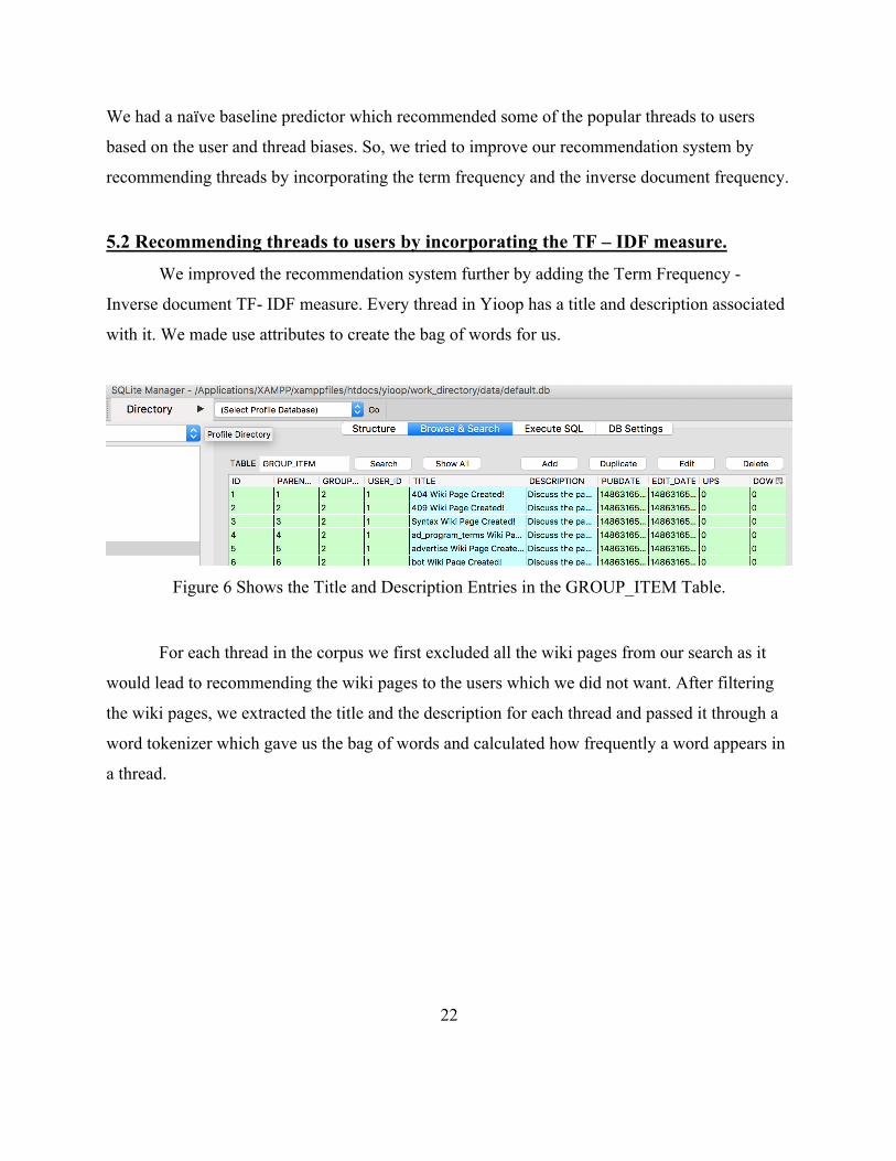
We improved the recommendation system further by adding the Term Frequency -

Inverse document TF- IDF measure. Every thread in Yioop has a title and description associated

with it. We made use attributes to create the bag of words for us.

Figure 6 Shows the Title and Description Entries in the GROUP_ITEM Table.

For each thread in the corpus we first excluded all the wiki pages from our search as it

would lead to recommending the wiki pages to the users which we did not want. After filtering

the wiki pages, we extracted the title and the description for each thread and passed it through a

word tokenizer which gave us the bag of words and calculated how frequently a word appears in

a thread.

23

Figure 7 Shows the Bag of Words Built from the Title and Description attributes.

5.2.1 Calculating the term frequency for each thread.

The GROUP_ITEM table in Yioop has the description of a thread and has attributes like

title, description, date published, group admin, the id of the group it belonged to, etc. We

scanned through each thread extracting the title and the description, followed by tokenizing the

words. While tokenizing we also kept a count of the number of times a word occurs in the thread

description and title. We also maintained a WORDS table which maintained the list of words.

So, whenever we found a new word in the thread scan we append it to the words list. Thus, we

got a count of the frequency of terms in the threads. As mentioned in the Term frequency

section, we saved the log of the term frequency to lessen the effect of the size of the title or

description.

TermFrequencyTF(items) = 𝑙𝑜𝑔 𝑓E,F + 1𝑖𝑓𝑓E,F > 0𝑎𝑛𝑑0𝑜𝑡ℎ𝑒𝑟𝑤𝑖𝑠𝑒

24

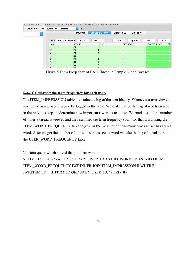
Figure 8 Term Frequency of Each Thread in Sample Yioop Dataset.

5.2.2 Calculating the term frequency for each user.

The ITEM_IMPRESSSION table maintained a log of the user history. Whenever a user viewed

any thread in a group, it would be logged in the table. We make use of the bag of words created

in the previous steps to determine how important a word is to a user. We made use of the number

of times a thread is viewed and then summed the term frequency count for that word using the

ITEM_WORD_FREQUENCY table to give us the measure of how many times a user has seen a

word. After we get the number of times a user has seen a word we take the log of it and store in

the USER_WORD_FREQUENCY table.

The join query which solved this problem was:

SELECT COUNT (*) AS FREQUENCY, USER_ID AS UID, WORD_ID AS WID FROM

ITEM_WORD_FREQUENCY IWF INNER JOIN ITEM_IMPRESSION II WHERE

IWF.ITEM_ID = II. ITEM_ID GROUP BY USER_ID, WORD_ID

25

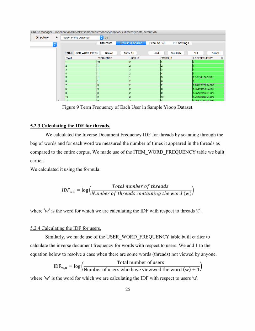
Figure 9 Term Frequency of Each User in Sample Yioop Dataset.

5.2.3 Calculating the IDF for threads.

We calculated the Inverse Document Frequency IDF for threads by scanning through the

bag of words and for each word we measured the number of times it appeared in the threads as

compared to the entire corpus. We made use of the ITEM_WORD_FREQUENCY table we built

earlier.

We calculated it using the formula:

𝐼𝐷𝐹x,E = log𝑇𝑜𝑡𝑎𝑙𝑛𝑢𝑚𝑏𝑒𝑟𝑜𝑓𝑡ℎ𝑟𝑒𝑎𝑑𝑠

𝑁𝑢𝑚𝑏𝑒𝑟𝑜𝑓𝑡ℎ𝑟𝑒𝑎𝑑𝑠𝑐𝑜𝑛𝑡𝑎𝑖𝑛𝑖𝑛𝑔𝑡ℎ𝑒𝑤𝑜𝑟𝑑 𝑤

where ′𝑤′ is the word for which we are calculating the IDF with respect to threads ′𝑡′.

5.2.4 Calculating the IDF for users.

Similarly, we made use of the USER_WORD_FREQUENCY table built earlier to

calculate the inverse document frequency for words with respect to users. We add 1 to the

equation below to resolve a case when there are some words (threads) not viewed by anyone.

IDF|,} = logTotalnumberofusers

Numberofuserswhohaveviewwedtheword w + 1

where ′w′ is the word for which we are calculating the IDF with respect to users ′u′.

26

We store the user and the thread IDF calculated for each word in a table IDF.

Figure 10 IDF Table on Sample Yioop Dataset.

5.2.5 Calculating the weights TF*IDF

We multiply the TF * IDF for each word for the users and threads.

This helps us build the USER_WORD_WEIGHTS AND THE ITEM_WORD_WEIGHTS table.

These tables give us a measure of how important a word is to a user and how important that word

is to the thread.

Figure 11 Item Word Weights Table on Sample Yioop Dataset.

27

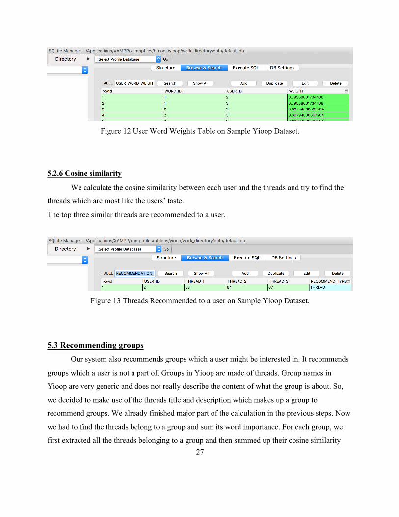
Figure 12 User Word Weights Table on Sample Yioop Dataset.

5.2.6 Cosine similarity

We calculate the cosine similarity between each user and the threads and try to find the

threads which are most like the users’ taste.

The top three similar threads are recommended to a user.

Figure 13 Threads Recommended to a user on Sample Yioop Dataset.

5.3 Recommending groups Our system also recommends groups which a user might be interested in. It recommends

groups which a user is not a part of. Groups in Yioop are made of threads. Group names in

Yioop are very generic and does not really describe the content of what the group is about. So,

we decided to make use of the threads title and description which makes up a group to

recommend groups. We already finished major part of the calculation in the previous steps. Now

we had to find the threads belong to a group and sum its word importance. For each group, we

first extracted all the threads belonging to a group and then summed up their cosine similarity

28

measure for a group. We then recommended the top three groups to a user which has the highest

weights.

Figure 14 Groups Recommended to a User on Sample Yioop Dataset.

5.4 Advantages of the TF – IDF method for Recommending threads/groups

The TF – IDF method for recommendation works very well for the Yioop Threads. The

method is very intuitive as we are trying to find out how much relevant a word is to a user based

on the number of times a user has viewed a word. Similarly, we are trying to find out how

important a word to a thread based on the frequency of the word in the thread. Thus, based on the

importance of the words to a user and a thread we can predict what a user would like to see – in

our case what are the threads or groups which he would like to be a part of.

29

6. RUNNING THE RECOMMENDATION JOB

We were dealing with a lot of data as each user, thread/group logs were being examined. If

we ran a recommendation job in the background all the time based on the new logs received, it

would slow down the computing power and there are chances that the computer might crash.

Hence, we came up with having two parts to the recommendation system. These two parts lead

to faster execution and recommended threads/groups to users instantly.

1. Offline Job – Computation Part

2. Online recommendations – Rendering Part

6.1 Offline Job – Computation Part A batched job is a job which runs for a data for a frame of time. As new logs keep

appending in Yioop. It will not be feasible to mine this huge corpus of data and expect it to

render correct results instantly. Yioop has a scalable framework media job which schedules job

and runs based on when it is scheduled. These jobs are periodic in nature [6] and have a very

efficient implementation. It can schedule jobs and process all files with a php extension. We

made an offline job for the recommendation system which makes the Yioop system learn about

the logs. We decided to run the recommendation job every week as it would gather a certain

number of logs which would have a considerable effect on our recommendations. So, we run the

recommendation job from the start date to now and consider all the logs and mine the data. We

build recommendation tables whose columns are user IDs followed by three columns which

states the top 3 threads/groups for recommendation.

The recommended threads are stored in RECOMMENDATION_LIST_THREADS_*

and groups are stored in RECOMMENDATION_LIST_GROUPS_* tables. The * tells us which

table is live. Here * takes the value of 1 or 2 depending on which table is live. It helps us in

giving recommendations even if the job is running in the background and the tables are being

updated. The table which is live is not affected at all while updating.

30

As one must have figured the offline job is the computationally intensive part of the

system. Most of the processing of the recommendation system is already done. The best part is

that this job is running offline, hence has no effect on the current recommendations or the

execution of Yioop.

6.2 Online Recommendations – Rendering Part

Once the tables are modified, the new recommendation table becomes live. When a user

signs in, then based on the user’s ID and the groups which a user is permitted to join he is

recommended with threads and groups.

The user is recommended with three items:

1. The three most trending groups based on the classic baseline predictor model we

built.

2. The three most interesting threads based on the words which he/she has viewed in the

past.

3. The three most interesting groups based on the words which he/she has viewed in the

past.

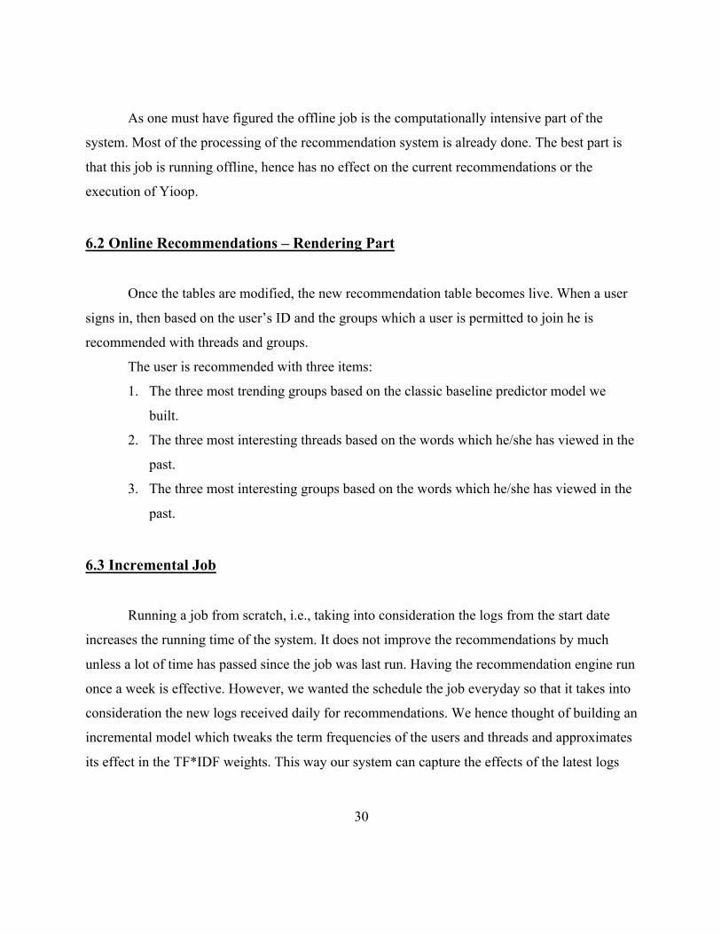
6.3 Incremental Job

Running a job from scratch, i.e., taking into consideration the logs from the start date

increases the running time of the system. It does not improve the recommendations by much

unless a lot of time has passed since the job was last run. Having the recommendation engine run

once a week is effective. However, we wanted the schedule the job everyday so that it takes into

consideration the new logs received daily for recommendations. We hence thought of building an

incremental model which tweaks the term frequencies of the users and threads and approximates

its effect in the TF*IDF weights. This way our system can capture the effects of the latest logs

31

and tweak the old weights calculated accordingly. It greatly reduces the running time if the job is

run daily.

Term frequency of the new users and threads can be captured by looking at the new logs

which we receive every day. However, the IDF calculation is affected whenever a new user is

added, a new thread is added or a user has viewed some new threads(words).

So, we do the approximation as given below,

we calculate the TF*IDF based on the newly seen records in the ITEM_IMPRESSION. We then

try to propagate the effect of this new TF*IDF into the old values by weights. For example, if

previously the TF*IDF was calculated on 100 users and a new user is added in the newly seen

data then for all the users who have seen some threads in the new set of logs are tweaked in the

following way. In our example, since the old weights were calculated on 100 users we multiply

the old weight with 100/101 and multiply the newly calculated weight by 1/100; and add the old

and the new weights.

There is a slight variation in the above approximations. We always add a constant 1

(dummy new user) in the equation because if no new users are added then the ratio 1/100 would

be 0 and the new TF*IDF would have no effect on the equation. The final equation for tweaking

the weights is as shown below:

TF ∗ IDF�,� =Totalnumberofoldusers

Totalnumberofoldandusers + 1 ∗ OLD TF ∗ IDF�,�

+Totalnumberofnewusers + 1

Totalnumberofoldandnewusers + 1 ∗ NEW TF ∗ IDF�,�

Also, since we are merely approximating, we run the online job from scratch after a

certain number of runs i.e., one week. So, in this way, we rebuild the tables with exact values

again.

32

7. USER INTERFACE

Yioop has a manage accounts page which lets the user to manage all his/her activities.

The user is directed to this page as soon as the user logs in. We decided to render our

recommendations on this page. Yioop uses the Model View Adapter design pattern [6]. So, the

entire codebase is divided into folders and sub folders based on the following classes:

1. Model – which handles all the data manipulations and definitions in the database

2. View – which is responsible for the rendering of the html pages

3. Controller – which handles the logic and the processing.

To render the pages, we had to modify the elements folder specifically

manageaccountelements.php which is a sub folder in views. We also had to define functions in

the User Model for providing the users with the recommendations by capturing the

recommendations from relevant tables.

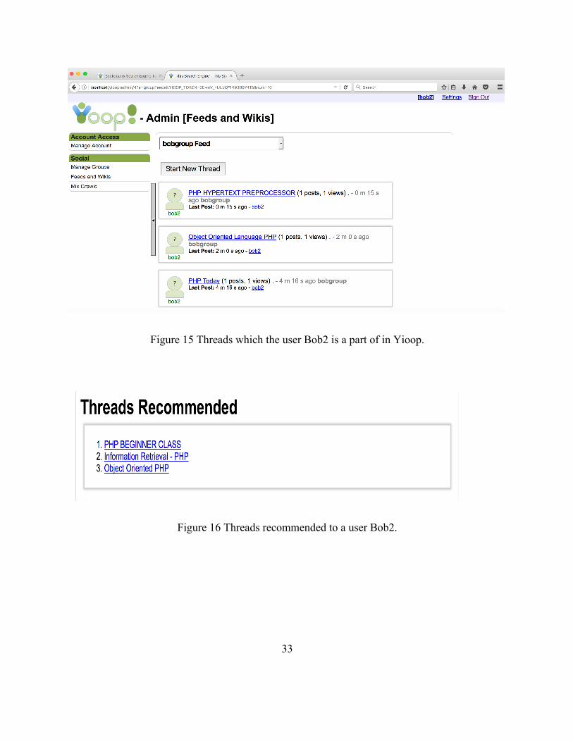
Let us try the recommendation system integrated with Yioop with very simple logs where

a user Bob2 watches only threads having one word. The Yioop user Bob2 is part of some of the

threads which is shown in the figure below. We make Bob2 to view all the threads which are

have the word PHP. Now, according to our model we want the recommendation system to

recommend some groups and threads having words like ‘PHP’ as Bob2 has frequently viewed

this word in the past. The figures show the threads and groups recommended to Bob2 and it

consists of the word ‘PHP’. Hence, we can conclude that we are recommending Bob2 with

threads and groups which are interesting to him.

33

Figure 15 Threads which the user Bob2 is a part of in Yioop.

Figure 16 Threads recommended to a user Bob2.

34

Figure 17 Groups recommended to a user Bob2.

Figure 18 Trending groups recommended to a user Bob2.

The actual user interface for recommendations in Yioop looks like this:

Figure 19 Recommendations given to a user in Yioop.

35

8. EXPERIMENTS AND TESTING

After integrating the recommendation system with Yioop we checked its effectiveness by

doing usability study. We tested our model by asking people who were users of Yioop as well as

some new users. 90 out of 100 people who tested this model had good reviews and had a better

website experience. They were recommended threads and groups which were relevant to their

taste.

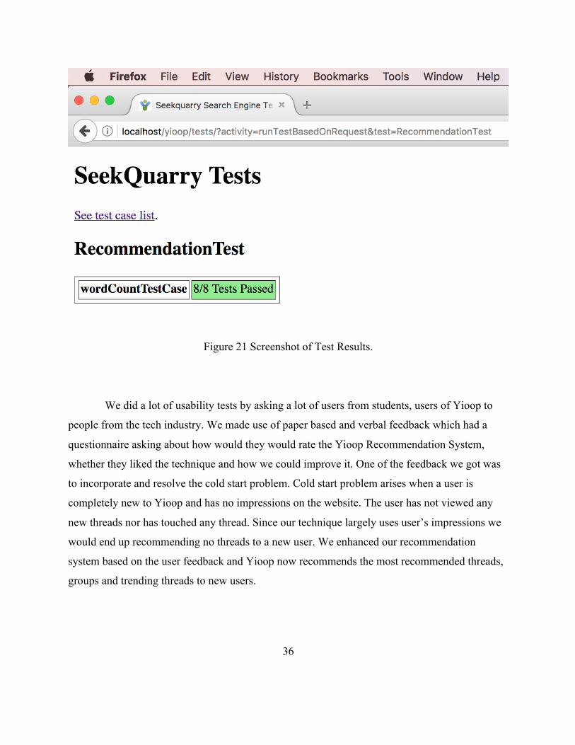
We also did some unit testing on the model using Yioop’s Testing Framework to check

for correctness of the words extraction and frequency count since that was the most important

function on which the entire bag of words was being created.

WordCountTestCase function – This function tested if the extracted title and description

from the GROUP_ITEM table did proper tokenization and returned the word frequency count

correctly.

Figure 20 Unit Testing Code to Check the Word Count.

For the rest of the computations we tried to handle most of the calculations in the

database for faster execution.

36

Figure 21 Screenshot of Test Results.

We did a lot of usability tests by asking a lot of users from students, users of Yioop to

people from the tech industry. We made use of paper based and verbal feedback which had a

questionnaire asking about how would they would rate the Yioop Recommendation System,

whether they liked the technique and how we could improve it. One of the feedback we got was

to incorporate and resolve the cold start problem. Cold start problem arises when a user is

completely new to Yioop and has no impressions on the website. The user has not viewed any

new threads nor has touched any thread. Since our technique largely uses user’s impressions we

would end up recommending no threads to a new user. We enhanced our recommendation

system based on the user feedback and Yioop now recommends the most recommended threads,

groups and trending threads to new users.

37

9. CONCLUSIONS AND FUTURE WORK

We researched the following techniques to build recommendation systems: Collaborative

Filtering, Content Based Filtering in brief, Latent Matrix Factorization. We studied the

collaborative filtering techniques in depth and tried to figure out what would be the best

technique for recommending threads/groups in Yioop. We researched Collaborative filtering –

baseline predictors and latent matrix factorization in depth. We also studied various ranking

algorithms which could help in the prediction. We started off building a recommender system

using the baseline predictor technique. Later, we realized that it recommended only the most

popular threads/ groups to the users. We improved our recommendation system by incorporating

the term frequency and the inverse document frequency in to our model. One of the challenges of

this project was to figure out a way to rate a thread as no user could give a numeric rating to a

thread/group. We made use users viewing history to convert it into a rating a user would give to

a thread. For the term frequency inverse document frequency, we made use of the fact of the

number of times a user views a word to calculate the metrics.

We implemented the recommendation system and integrated it with Yioop to recommend

the most popular threads/groups and the most relevant threads/groups based on users viewing

history. We built a User interface which rendered the recommendations as soon as the user

logged in. We also tested our model by performing unit testing on a few functions to check if it

calculated the metrics correctly. To test the effectiveness, we asked several users to try our

recommendation system and give their opinion. The response was positive from most of the

users nearly 90 percent users gave a positive feedback.

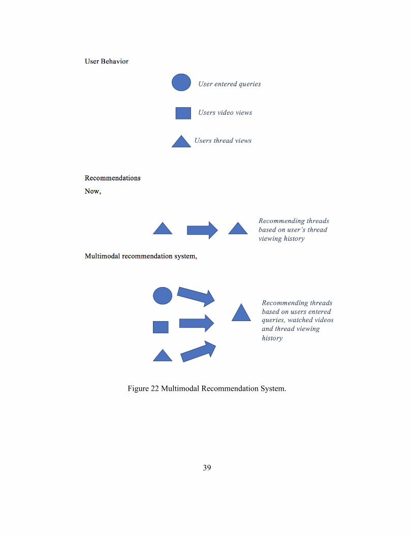
9.1 Multimodal Recommendations

Multimodal recommendations make use of a variety of user’s behavior to make

recommendations [7]. For our project, we have only made use of a user’s viewing patterns in the

past to make recommendations. However, there are a lot of other things which a user does in

Yioop like watching videos, querying the search engine, posting discussions, etc. which we can

incorporate in our recommendation system.

38

Every minute click a user does on a website says a lot about the user and his interests. We

can extend this project to incorporate those behaviors and make the recommendations more

relevant.

The figure gives an overview of how we are recommending threads or groups to users

now, and how can it make use of the other user behaviors to extend the recommendation model

to make a multimodal recommendation system.

39

Figure 22 Multimodal Recommendation System.

40

10. BIBLIOGRAPHY

[1] P. Resnick and H. R. Varian, “Recommender systems,” Communications of the ACM, vol.

40, no. 3, pp. 56–58, 1997.

[2] Ramos, Juan. "Using TF-IDF to Determine Word Relevance in Document Queries." [Online].

Available:

http://citeseerx.ist.psu.edu/viewdoc/download?doi=10.1.1.121.1424&rep=rep1&type=pdf

[Accessed: 02 - May- 2017].

[3] Koren, Yehuda. The BellKor Solution to the Netflix Grand Prize (2009). [Online]. Available:

http://www.netflixprize.com/assets/GrandPrize2009_BPC_BellKor.pdf


[4] "Netflix Prize." Wikipedia. Wikimedia Foundation. [Online]. Available:

https://en.wikipedia.org/wiki/Netflix_Prize [Accessed: 02 - May- 2017].

[5] "Term Frequency and Weighting." Term Frequency and Weighting. Cambridge University

Press, 2008. [Online]. Available:

https://nlp.stanford.edu/IR-book/html/htmledition/term-frequency-and-weighting-1.html


[6] Seekquarry.com, “Resources,” 2015. [Online]. Available:

https://www.seekquarry.com/p/Resources. [Accessed: 02 - May- 2017].

[7] Dunning, Ted, and B. Ellen Friedman. Practical Machine Learning: Innovations in

Recommendation. Beijing: O'Reilly, 2014. Print.

[8] Langville, A. N., & Meyer, C. D. (2012). Who's #1? The science of rating and ranking.

Princeton: Princeton University Press.

41

[9] Cormen, T. H., Leiserson, C. E., & Rivest, R. L. (1990). Introduction to algorithms.

Cambridge, MA: MIT Press.

[10] Gábor Takács , István Pilászy , Bottyán Németh , Domonkos Tikk, Major components of

the gravity recommendation system, ACM SIGKDD Explorations Newsletter, v.9 n.2, December

2007 [doi>10.1145/1345448.1345466]

An Open Source Discussion Group Recommendation … · III The Designated Project Committee Approves...

Documents

Transcript of An Open Source Discussion Group Recommendation … · III The Designated Project Committee Approves...