An Invitation to Fractal Geometry and Its Applications
33
An Invitation to Fractal Geometry and Its Applications Michel L. Lapidus, Dana Clahane, Robert G. Niemeyer University of California, Riverside Department of Mathematics 900 Big Springs Rd. Riverside, CA, 92521 [email protected], [email protected], [email protected] (Draft Version) October 7, 2006
-
Upload
pals4ever143 -
Category
Documents
-
view
61 -
download
4
Transcript of An Invitation to Fractal Geometry and Its Applications
An Invitation to Fractal
Geometry and Its Applications
Michel L. Lapidus, Dana Clahane, Robert G. Niemeyer
University of California, Riverside
Department of Mathematics
900 Big Springs Rd.
Riverside, CA, 92521
[email protected], [email protected], [email protected]
(Draft Version)
October 7, 2006

2
Contents
1 Introduction 7
2 Preliminaries 9
2.1 Complex Numbers . . . . . . . . . . . . . . . . . . . . . . . . . . 9
2.2 Set-Theoretic Notation and Concepts . . . . . . . . . . . . . . . . 16
2.3 Calculus . . . . . . . . . . . . . . . . . . . . . . . . . . . . . . . . 16
2.4 Point-Set Topology and Metric Spaces . . . . . . . . . . . . . . . 23
3 Concepts in Fractal Geometry 25
3.1 Euclidean Generators . . . . . . . . . . . . . . . . . . . . . . . . . 29
3.2 Recursion and Fractal Construction . . . . . . . . . . . . . . . . 31
3.3 Self-Similar and Self-Affinity . . . . . . . . . . . . . . . . . . . . . 36
3.4 Infinite Length and Uncountability . . . . . . . . . . . . . . . . . 45
3.5 Non-Integer Dimension . . . . . . . . . . . . . . . . . . . . . . . . 49
3.6 Various Fractal Dimensions . . . . . . . . . . . . . . . . . . . . . 51
3.7 Summary . . . . . . . . . . . . . . . . . . . . . . . . . . . . . . . 51
3
4 CONTENTS
4 Measure Theory 53
5 Dimension theory (intuitive approach...box counting and Haus-
dorff) 57
5.0.1 Self-Similarity Dimension . . . . . . . . . . . . . . . . . . 58
5.0.2 Box-Counting Dimension . . . . . . . . . . . . . . . . . . 61
6 Iterated Function Systems 63
7 Fractal Curves and Sets 65
7.1 Fractal Criteria . . . . . . . . . . . . . . . . . . . . . . . . . . . . 65
7.2 Taming the Mathematical Monsters . . . . . . . . . . . . . . . . 68
7.2.1 Nondifferentiability of the Weierstrass Function . . . . . . 70
7.3 Definitions for a Fractal (many competing ones and the definitions) 78
8 Fractal Strings 79
9 Calculus on Fractals (i.e. lite analysis on fractals) 81
10 Applications 83
10.1 Brownian Motions . . . . . . . . . . . . . . . . . . . . . . . . . . 83
10.1.1 Theoretical Interpretation . . . . . . . . . . . . . . . . . . 84
10.1.2 Fractal Properties of Brownian Paths & Graphs . . . . . 92
10.2 Fractal Economics (Mandelbrot’s work) . . . . . . . . . . . . . . 95
10.3 Fractal Biology . . . . . . . . . . . . . . . . . . . . . . . . . . . . 95
10.4 Fractals in Physics . . . . . . . . . . . . . . . . . . . . . . . . . . 95
CONTENTS 5
10.5 Fractals in cognition,sociology (Dr. Lapidus has a book on shelf) 95
10.6 Fractal Drums . . . . . . . . . . . . . . . . . . . . . . . . . . . . 95
10.7 Fractal Billiards . . . . . . . . . . . . . . . . . . . . . . . . . . . . 95
• Historical significance
• Intuitive motivation
• Intuitive motivation for fractals
• Outline of chapter
Chapter 3
Concepts in Fractal
Geometry
Fractal Geometry has its roots in a variety of analytical problems. Many of the
standard sets found in every fractal geometer’s tool box were originally discussed
in the context of counter-examples to long-standing problems. In some cases,
the development of fractal sets were in answer to physical problems.
The early work of Fourier on heat diffusion and harmonic analysis motivated
Riemann, Weierstrass and others to investigate the analytic nature of explicit
trigonometric series. As a result of Riemann and Weierstrass’ separate works, it
was settled once and for all that highly nondifferentiable and entirely nondiffer-
entiable functions did exist. In fact, the mathematical community was quickly,
though begrudgingly, conceding that nondifferentiable functions were the norm
25
26 Chapter 3. Concepts in Fractal Geometry
and differentiable functions were a special case. But this was just the beginning
of a deep mathematical mystery.
Cantor was a contemporary of Weierstrass and did much to create an up-
heaval in mathematics, as well. In particular, his discoveries led to a recon-
ceptualization of similarity. While his original results were concerned with Set
Theory and Harmonic Analysis, his name is now pervasive in many mathemati-
cal branches. In fact, his famous Cantor set is the first “monster” many students
are introduced to, mainly because it is a perfect set with Lebesgue measure zero
and cardinality equal to that of the unit interval.
The generation after Weierstrass and Cantor included Giuseppe Peano, Helge
von Koch, Waclaw Sierpinski, and others, each having a surprise of their own.
Peano shook the geometric intuition of every mathematician when he demon-
strated that there exists a continuous map f from the unit interval I to the unit
square I × I whose image fills the space I × I.
Von Koch’s example of a nowhere differentiable function was borne out of a
desire to have a more natural example of Weierstrass’ findings.
Waclaw Sierpinski, while known to budding fractal geometers for his Sierpin-
ski gasket made an astonishing discovery with the Sierpinski carpet. He found
that any planar Jordan curve could be embedded homeomorphically into the
Sierpinski carpet. Though this fact did not hold for the Sierpinski gasket, Karl
Menger was able to extend the results to higher dimensions.
Around the time of Sierpinski and Menger, Wiener was placing the work of
Robert Brown, Albert Einstein and others on a rigorous foundation. Brownian
27
paths and motion, as formalized by Wiener were nondifferentiable paths and
physical Brownian motion was the expression of a naturally occurring statisti-
cally self-similar fractal.
For years, physicists have been developing methods to explain geometric
phenomena that were not fitting well with traditional Euclidean concepts. As
a field, Fractal Geometry cannot be described as a purely theoretical study
of fractal sets, nor can insight be gained by rephrasing it as ‘the geometry of
fractals,’ if such a concept were even rigorously defined. Nor is it an area entirely
devoted to explaining roughness in Nature. Rather, Fractal Geometry is the
unification of seemingly unrelated fields under an umbrella of pure mathematics
that ties together the various concepts in the physical sciences by providing a
rigorous mathematical foundation.
More recent motivation for developing the study of fractal sets came from
Benoit B. Mandelbrot’s paper, How long is the coast of Britain [16], and the
culmination of his work in the treatise, The Fractal Geometry of Nature [13]. In
such works, the nature of roughness was closely examined and placed on a more
rigorous foundation. For example, the shoreline seems rather smooth at large
scales, but any attempt to measure the coast shows that finer and finer scales
only illuminate the shore’s roughness and make the length longer and longer.
Topologically speaking, a fractal and non-fractal curve are equivalent. The
first attempt at developing a method for discerning was made by Felix Hausdorff.
Though Hausdorff is a name traditionally associated with particular topological
spaces, the topologically noninvariant method developed by Hausdorff entailed
28 Chapter 3. Concepts in Fractal Geometry
assigning a value to a set that indicated a point at which the measure of a set
jumped from infinity to zero. As part of the goal of research, mathematicians
now attempt to classify sets in a non-topological manner so as to provide a well-
defined method for differentiating between two topologically equivalent sets.
For over forty years, mathematicians have been confronted with the problem
of what constitutes a fractal set. The word fractal, having its origins in the Latin
word for broken - fractus - was coined by Benoit Mandelbrot. The following
fractal criteria was set forth by Mandelbrot.
Criteria 3.0.1 ( [13]). “A fractal is, by definition, a set for which the Hausdorff–
Besicovitch dimension strictly exceeds the topological dimension.”
This definition was later dismissed by Mandelbrot as being insufficient in its
ability to describe a larger class of sets that the intellectual community accepted
as being fractal. In particular, this definition excluded the Devil’s Staircase.
Hence, Mandelbrot next proposed that a fractal be defined as follows:
Criteria 3.0.2 ( [17]). A fractal is a shape made of parts similar to the whole
in some way.
Researchers across the various scientific disciplines readily agreed that this
was a better definition for fractal, but was still inadequate for rigorous mathe-
matical discussion (see [14]).
One main problem in the discipline thus far is the lack of an official rigorous
definition for fractal. While research in this area will be discussed and analyzed,
we shall first introduce the various criteria used to decide whether or not a set
3.1. Euclidean Generators 29
is fractal.
Before we discuss the various fractal criteria, it is extremely important to
realize that a fractal set F cannot be illustrated in reality. This stems from
the fact that Nature is discrete. Eventually the granular nature of matter rears
its ugly head and shows that everything is not smooth at some fixed scale.
For example, a smooth curve drawn on paper will exhibit a high degree of
roughness at the microscopic scale. Another example is the fern. At some level,
the fern ceases to exist as a ‘self-repeating’ structure and the cellular structure
becomes apparent. Hence, the fern has a limited self-similar structure. What
is important is that the abstract knowledge gained in the study of what are
termed self-similar sets offers insight into finitely self-similar structures.
3.1 Euclidean Generators
Traditional Euclidean shapes are points (a1, a2, ..., an), lines #»r , n-spheres, and
n-dimensional polyhedra. Such shapes are finite in their measure and can be
unioned and intersected in such a way so as to produce more complicated Eu-
clidean shapes. Furthermore, Euclidean shapes, are used in the construction of
fractal sets. However, this does not imply that a fractal is merely a complicated
Euclidean shape in disguise.
A fractal can often be constructed by a particular iterative process that
begins with an initiator and/or generator. The initiator and generator are rep-
resented by the familiar Euclidean shapes, i.e. line segments, circles, polygons
30 Chapter 3. Concepts in Fractal Geometry
and polyhedra. The initiator and generator of most of the fractals that we will
discuss will be line segments. The generator is constructed from the initiator,
and then the fractal is constructed from the generator in accordance with a
particular iterative process. After each successive iteration, the shape loses its
traditional Euclidean appearance and, in the limit, becomes a fractal set.
Definition 3.1.1 (Prefractal). If a set X of points is the nth level approxi-
mation of a fractal F , then X is called a prefractal. In particular, X is the
prefractal Fn.
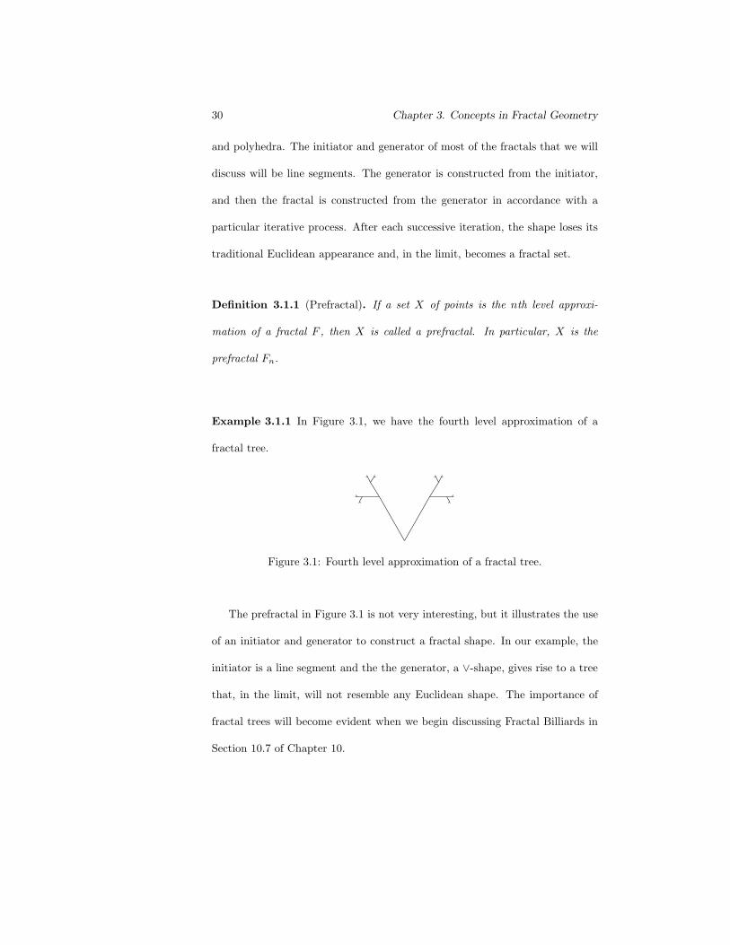
Example 3.1.1 In Figure 3.1, we have the fourth level approximation of a
fractal tree.
Figure 3.1: Fourth level approximation of a fractal tree.
The prefractal in Figure 3.1 is not very interesting, but it illustrates the use
of an initiator and generator to construct a fractal shape. In our example, the
initiator is a line segment and the the generator, a ∨-shape, gives rise to a tree
that, in the limit, will not resemble any Euclidean shape. The importance of
fractal trees will become evident when we begin discussing Fractal Billiards in
Section 10.7 of Chapter 10.
3.2. Recursion and Fractal Construction 31
3.2 Recursion and Fractal Construction
Definition 3.2.1 (Recursion). The process of defining an object in terms of
itself.
Definition 3.2.2 (Algorithm). An algorithm is a fnite set of precise instruc-
tions for performing a computation, for describing a set, or for solving a prob-
lem.
In our discussion, we will mostly be using the word algorithm in the context
of describing a set. From these two definitions, it is clear what a recursively
defined algorithm is.
Definition 3.2.3 (Recursively Defined Algorithm). A finite set of instructions
for which the output of the algorithm is used as input for the same algorithm.
For many fractals, there are many options for symbolically representing the
algorithmic construction. In particular, we will focus on the use of L-Systems
for describing the construction of a variety of fractal sets.
L-Systems, named after the botanist Aristid Lindenmayer, is a formal lan-
guage used to describe the formation of plants. In his research, Lindenmayer
defined variables and operations that served as input for a computer, which
would then output a fairly detailed rendition of the plant. Abstractly, the con-
struction of any object which exhibits self-similarity or self-affineness can be
described by a particular L-system, meaning that every self-similar or self-affine
fractal can be described by a particular L-system. However, computational
restraints restrict an L-system from realistically describing a fractal F .
32 Chapter 3. Concepts in Fractal Geometry
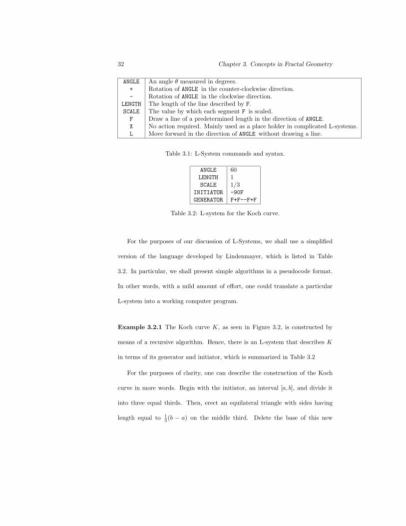
ANGLE An angle θ measured in degrees.+ Rotation of ANGLE in the counter-clockwise direction.- Rotation of ANGLE in the clockwise direction.
LENGTH The length of the line described by F.SCALE The value by which each segment F is scaled.F Draw a line of a predetermined length in the direction of ANGLE.X No action required. Mainly used as a place holder in complicated L-systems.L Move forward in the direction of ANGLE without drawing a line.
Table 3.1: L-System commands and syntax.
ANGLE 60LENGTH 1SCALE 1/3
INITIATOR -90F
GENERATOR F+F--F+F
Table 3.2: L-system for the Koch curve.
For the purposes of our discussion of L-Systems, we shall use a simplified
version of the language developed by Lindenmayer, which is listed in Table
3.2. In particular, we shall present simple algorithms in a pseudocode format.
In other words, with a mild amount of effort, one could translate a particular
L-system into a working computer program.
Example 3.2.1 The Koch curve K, as seen in Figure 3.2, is constructed by
means of a recursive algorithm. Hence, there is an L-system that describes K
in terms of its generator and initiator, which is summarized in Table 3.2
For the purposes of clarity, one can describe the construction of the Koch
curve in more words. Begin with the initiator, an interval [a, b], and divide it
into three equal thirds. Then, erect an equilateral triangle with sides having
length equal to 13 (b − a) on the middle third. Delete the base of this new
3.2. Recursion and Fractal Construction 33
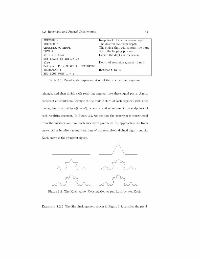
INTEGER i Keep track of the recursion depth.INTEGER r The desired recursion depth.CHAR STRING SHAPE The string that will contain the data.LOOP i Start the looping process.if i = 0 then Decide the depth of recursion.Set SHAPE to INITIATOR
else Depth of recursion greater than 0.Set each F in SHAPE to GENERATOR
INCREMENT i Increase i by 1.END LOOP WHEN i = r
Table 3.3: Pseudocode implementation of the Koch curve L-system.
triangle, and then divide each resulting segment into three equal parts. Again,
construct an equilateral triangle at the middle third of each segment with sides
having length equal to 13 (b′ − a′), where b′ and a′ represent the endpoints of
each resulting segment. In Figure 3.2, we see how the generator is constructed
from the initiator and how each successive prefractal Kn approaches the Koch
curve. After infinitely many iterations of the recursively defined algorithm, the
Koch curve is the resultant figure.
Figure 3.2: The Koch curve. Construction as put forth by von Koch.
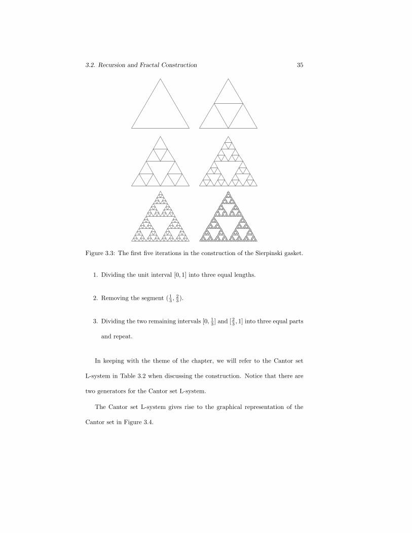
Example 3.2.2 The Sierpinski gasket, shown in Figure 3.3, satisfies the previ-
34 Chapter 3. Concepts in Fractal Geometry
ously discussed criteria, as listed below.
• The Sierpinski gasket is self-similar, since it is the result of the union of a
finite number of similarity transformations.
• The generator of the Sierpinski gasket is an equilateral triangle.
• The Sierpinski gasket can be constructed by way of a recursive algorithm,
as listed in Table 3.2.
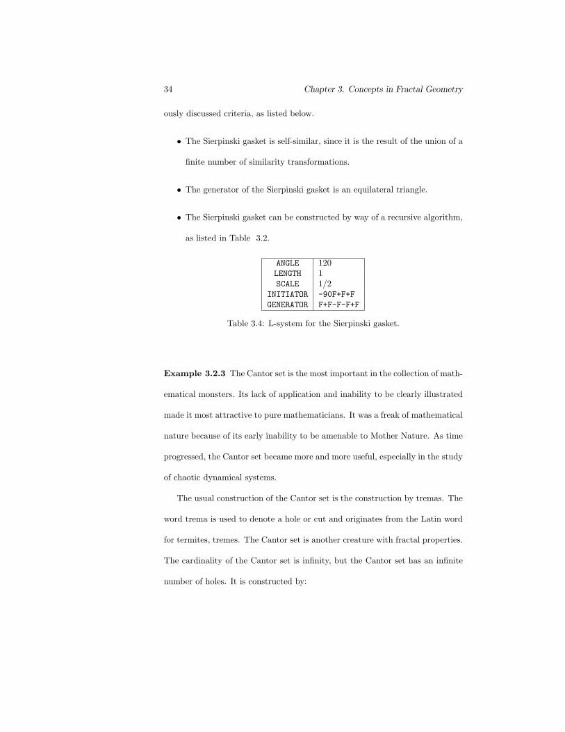
ANGLE 120LENGTH 1SCALE 1/2
INITIATOR -90F+F+F
GENERATOR F+F-F-F+F
Table 3.4: L-system for the Sierpinski gasket.
Example 3.2.3 The Cantor set is the most important in the collection of math-
ematical monsters. Its lack of application and inability to be clearly illustrated
made it most attractive to pure mathematicians. It was a freak of mathematical
nature because of its early inability to be amenable to Mother Nature. As time
progressed, the Cantor set became more and more useful, especially in the study
of chaotic dynamical systems.
The usual construction of the Cantor set is the construction by tremas. The
word trema is used to denote a hole or cut and originates from the Latin word
for termites, tremes. The Cantor set is another creature with fractal properties.
The cardinality of the Cantor set is infinity, but the Cantor set has an infinite
number of holes. It is constructed by:
3.2. Recursion and Fractal Construction 35
Figure 3.3: The first five iterations in the construction of the Sierpinski gasket.
1. Dividing the unit interval [0, 1] into three equal lengths.
2. Removing the segment ( 13 , 2
3 ).
3. Dividing the two remaining intervals [0, 13 ] and [23 , 1] into three equal parts
and repeat.
In keeping with the theme of the chapter, we will refer to the Cantor set
L-system in Table 3.2 when discussing the construction. Notice that there are
two generators for the Cantor set L-system.
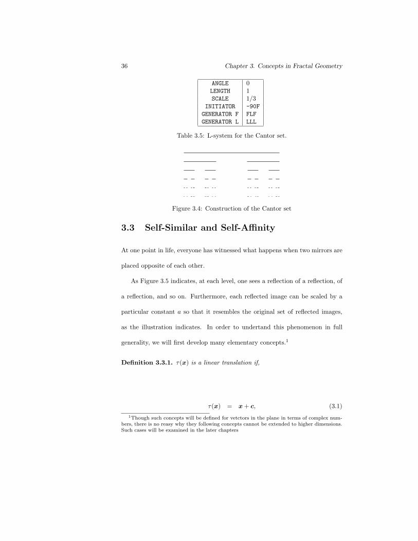
The Cantor set L-system gives rise to the graphical representation of the
Cantor set in Figure 3.4.
36 Chapter 3. Concepts in Fractal Geometry
ANGLE 0LENGTH 1SCALE 1/3
INITIATOR -90F
GENERATOR F FLF
GENERATOR L LLL
Table 3.5: L-system for the Cantor set.
Figure 3.4: Construction of the Cantor set
3.3 Self-Similar and Self-Affinity
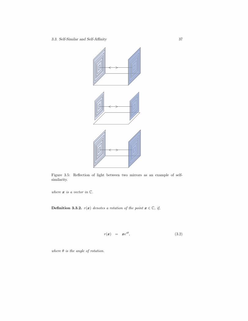
At one point in life, everyone has witnessed what happens when two mirrors are
placed opposite of each other.
As Figure 3.5 indicates, at each level, one sees a reflection of a reflection, of
a reflection, and so on. Furthermore, each reflected image can be scaled by a
particular constant a so that it resembles the original set of reflected images,
as the illustration indicates. In order to undertand this phenomenon in full
generality, we will first develop many elementary concepts.1
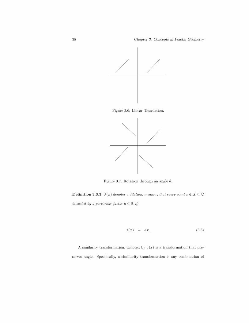
Definition 3.3.1. τ(x) is a linear translation if,
τ(x) = x + c, (3.1)
1Though such concepts will be defined for vetctors in the plane in terms of complex num-bers, there is no reasy why they following concepts cannot be extended to higher dimensions.Such cases will be examined in the later chapters
3.3. Self-Similar and Self-Affinity 37
Figure 3.5: Reflection of light between two mirrors as an example of self-similarity.
where x is a vector in C.
Definition 3.3.2. r(x) denotes a rotation of the point x ∈ C, if,
r(x) = xeiθ, (3.2)
where θ is the angle of rotation.
38 Chapter 3. Concepts in Fractal Geometry
Figure 3.6: Linear Translation.
Figure 3.7: Rotation through an angle θ.
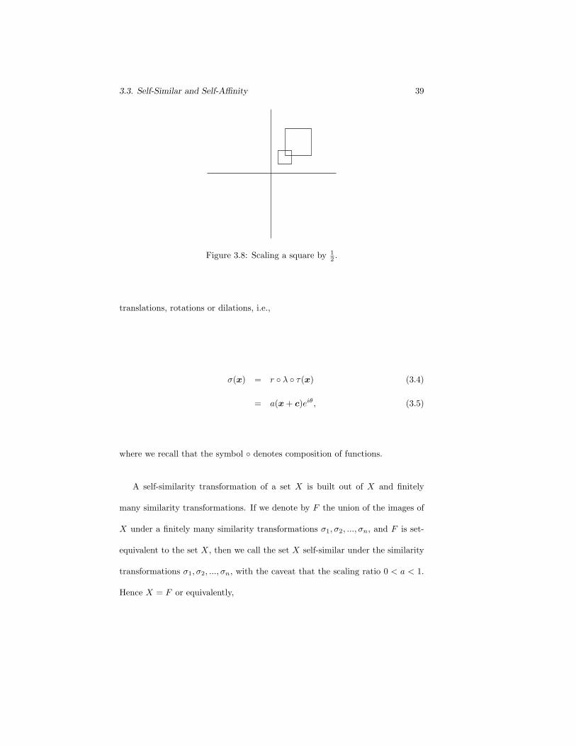
Definition 3.3.3. λ(x) denotes a dilation, meaning that every point x ∈ X ⊆ C
is scaled by a particular factor a ∈ R if,
λ(x) = ax. (3.3)
A similarity transformation, denoted by σ(x) is a transformation that pre-
serves angle. Specifically, a similiarity transformation is any combination of
3.3. Self-Similar and Self-Affinity 39
Figure 3.8: Scaling a square by 12 .
translations, rotations or dilations, i.e.,
σ(x) = r ◦ λ ◦ τ(x) (3.4)
= a(x + c)eiθ, (3.5)
where we recall that the symbol ◦ denotes composition of functions.
A self-similarity transformation of a set X is built out of X and finitely
many similarity transformations. If we denote by F the union of the images of
X under a finitely many similarity transformations σ1, σ2, ..., σn, and F is set-
equivalent to the set X, then we call the set X self-similar under the similarity
transformations σ1, σ2, ..., σn, with the caveat that the scaling ratio 0 < a < 1.
Hence X = F or equivalently,
40 Chapter 3. Concepts in Fractal Geometry
X = σ1(F ) ∪ σ2(F ) ∪ ... ∪ σn(F ) (3.6)
More to the point, any set constructed by means of a self-similarity transforma-
tion is self-similar.
Unfortunately, as a tool for discerning a shape’s fractality, the definition of
self-similarity is too restrictive. Hence, we must develop a more general concept
of self-similarity that includes a larger class of sets. This concept is called self-
affinity.
An affine transformation is a similarity transformation with the added qual-
ity of shearing.
Definition 3.3.4 (Shear – Horizontal Line Preserving). Every point (x0, y0) in
the plane is translated along a vertical line y = y0 that is parallel to a particular
fixed line in the plane, i.e.,
s[(x, y)] = (tx, y) + c (3.7)
where t ∈ R
Definition 3.3.5 (Shear – Vertical Line Preserving). Every point (x0, y0) in
the plane is translated along a vertical line x = x0 that is parallel to a particular
fixed line in the plane, i.e.,
3.3. Self-Similar and Self-Affinity 41
s[(x, y)] = (x, uy) + c (3.8)
where u ∈ R
Definition 3.3.6 (Shear). Every point (x, y) in the plane is translated along a
line that is parallel to a particular fixed line in the plane, i.e.,
s[(x, y)] = (tx, uy) + c (3.9)
where t, u ∈ R and 0 < t < 1, 0 < u < 1.
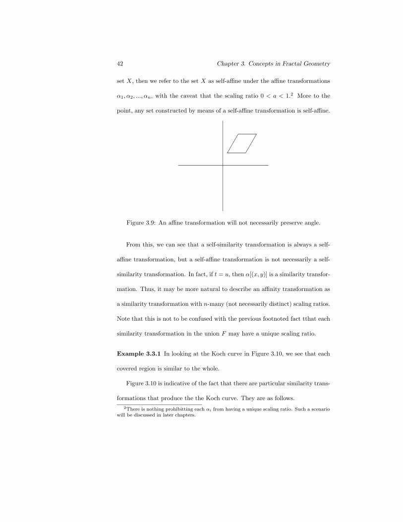
For example, one can rotate, translate and scale a square, but shearing will
cause the square to become a rhombus. Thus, affine transformations do not
necessarily preserve angle. The following is the form of an affine tranformation
in full generality.
α((x, y)) = r ◦ s((x, y)) (3.10)
= [(tx, uy) + c]eiθ (3.11)
Much like the concept of self-similarity, a self-affine transformation of a set
X is a specific type of affine transformation. If we denote the union of a finite
number of affine transformation α1, α2, ..., αn by F and F is set-equivalent to the
42 Chapter 3. Concepts in Fractal Geometry
set X, then we refer to the set X as self-affine under the affine transformations
α1, α2, ..., αn, with the caveat that the scaling ratio 0 < a < 1.2 More to the
point, any set constructed by means of a self-affine transformation is self-affine.
Figure 3.9: An affine transformation will not necessarily preserve angle.
From this, we can see that a self-similarity transformation is always a self-
affine transformation, but a self-affine transformation is not necessarily a self-
similarity transformation. In fact, if t = u, then α[(x, y)] is a similarity transfor-
mation. Thus, it may be more natural to describe an affinity transformation as
a similarity transformation with n-many (not necessarily distinct) scaling ratios.
Note that this is not to be confused with the previous footnoted fact tthat each
similarity transformation in the union F may have a unique scaling ratio.
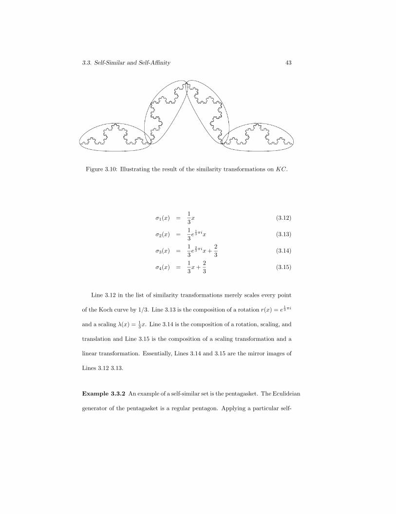
Example 3.3.1 In looking at the Koch curve in Figure 3.10, we see that each
covered region is similar to the whole.
Figure 3.10 is indicative of the fact that there are particular similarity trans-
formations that produce the the Koch curve. They are as follows.
2There is nothing prohibitting each αi from having a unique scaling ratio. Such a scenariowill be discussed in later chapters.
3.3. Self-Similar and Self-Affinity 43
Figure 3.10: Illustrating the result of the similarity transformations on KC.
σ1(x) =1
3x (3.12)
σ2(x) =1
3e
13 πix (3.13)
σ3(x) =1
3e
23 πix +
2
3(3.14)
σ4(x) =1
3x +
2
3(3.15)
Line 3.12 in the list of similarity transformations merely scales every point
of the Koch curve by 1/3. Line 3.13 is the composition of a rotation r(x) = e13 πi
and a scaling λ(x) = 13x. Line 3.14 is the composition of a rotation, scaling, and
translation and Line 3.15 is the composition of a scaling transformation and a
linear transformation. Essentially, Lines 3.14 and 3.15 are the mirror images of
Lines 3.12 3.13.
Example 3.3.2 An example of a self-similar set is the pentagasket. The Eculideian
generator of the pentagasket is a regular pentagon. Applying a particular self-
44 Chapter 3. Concepts in Fractal Geometry
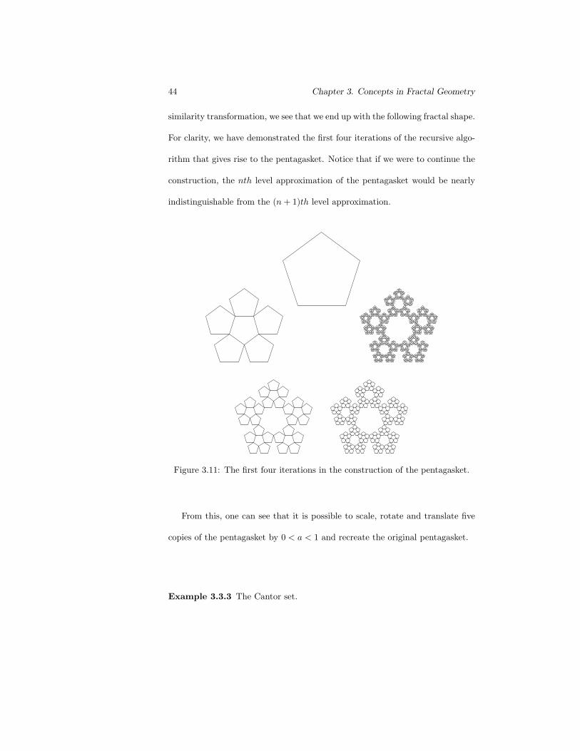
similarity transformation, we see that we end up with the following fractal shape.
For clarity, we have demonstrated the first four iterations of the recursive algo-
rithm that gives rise to the pentagasket. Notice that if we were to continue the
construction, the nth level approximation of the pentagasket would be nearly
indistinguishable from the (n + 1)th level approximation.
Figure 3.11: The first four iterations in the construction of the pentagasket.
From this, one can see that it is possible to scale, rotate and translate five
copies of the pentagasket by 0 < a < 1 and recreate the original pentagasket.
Example 3.3.3 The Cantor set.
3.4. Infinite Length and Uncountability 45
σ1(x) =x
3(3.16)
σ2(x) =x + 2
3(3.17)
3.4 Infinite Length and Uncountability
Definition 3.4.1 (Finite Set). If a set X has finitely many elements, then we
refer to the set as finite.
Definition 3.4.2 (Countably Infinite). If the elements of a set X can be put
into a bijective correspondence with the natural numbers, then we refer to the
set as countably infinite.
As will be shown later, in order to show something is not countable, it is
enough to show that any attempt to ‘list’ the elements results in at least one
element being unlistable.
Definition 3.4.3 (Uncountable). If a set X cannot be placed into a bijective
correspondence with the natural numbers and the set is not finite, then we refer
to the set X as uncountable.
As sets, most fractals are uncountable, and as geometric objects, it is usually
the case that a fractal will have infinite length. To demonstrate these qualities,
we will prove that the Cantor set is uncountable, and we will attempt to calculate
the length of the Sierpinski gasket and the Koch curve.
46 Chapter 3. Concepts in Fractal Geometry
Example 3.4.1 Since the Sierpinski gasket is constructed by means of an L-
system, we can view it as a curve and each iteration as a collection of line
segments in the plane. The first iteration of the Sierpinski gasket L-system
shows that the length of the curve is 9/2. The second iteration shows that the
length of SG2 is 27/4. From this, we would like to deduce that the length of
the Sierpinski gasket is 3(
32
)n.
Theorem 3.4.1 (Length of the prefractal SGn). If SGn is the nth level approx-
imation of the Sierpinski gasket, then the length of SGn is given by l(SGn) =
3(3/2)n.
Proof We shall proceed by induction. The trivial case is n = 1. The
prefractal SG1 does indeed have length 9/2. Suppose the length of SGn is
given by l(KCn) = 3(3/2)n for some fixed n. Then,
l(SGn+1) = l
(3
2SGn
)
=3
2l(SGn)
= 33
2
(3
2
)n
= 3
(3
2
)n+1
�
From this, we can see that as n → ∞, l(SGn) → ∞.
Example 3.4.2 By now, one should be familiar with the construction of the
3.4. Infinite Length and Uncountability 47
Koch curve. After the first iteration of the Koch curve L-system, there are four
segments each with length 1/3. After the second iteration, there are sixteen
segments of length 1/9. What we need to first prove is that the length of any
given prefractal KCn can be given by (4/3)n.
Theorem 3.4.2 (Length of the prefractal KCn). If KCn is the nth level ap-
proximation of the Koch curve, then the length of KCn is given by (4/3)n.
Proof We shall proceed by induction. The trivial case is n = 1. The
prefractal KC1 does indeed have length 4/3. Suppose the length of KCn is
given by (4/3)n for some fixed n. Then,
l(KCn+1) = l
(4
3KCn
)
=4
3l(KCn)
=4
3
(4
3
)n
=
(4
3
)n+1
�
From this, we can see that as n → ∞, l(KCn) → ∞.
Example 3.4.3 At first glance, Figure 3.4 would lead one to believe that C is
finite and not terribly large. However, the case is quite the contrary. Mandelbrot
referred to the Cantor set as Cantor dust because the visual representation leads
the reader to believe it is nothing more than specs of dirt laid out in a line. In
48 Chapter 3. Concepts in Fractal Geometry
fact, the Cantor set is an uncountable subset of the unit interval [1, 0] and has
measure zero, which will be proved later.
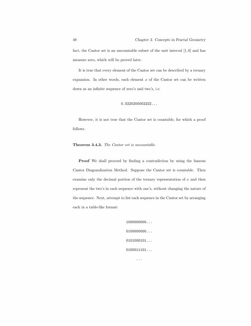
It is true that every element of the Cantor set can be described by a ternary
expansion. In other words, each element x of the Cantor set can be written
down as an infinite sequence of zero’s and two’s, i.e.
0.0220200002222...
However, it is not true that the Cantor set is countable, for which a proof
follows.
Theorem 3.4.3. The Cantor set is uncountable.
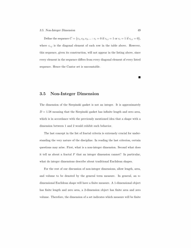
Proof We shall proceed by finding a contradiction by using the famous
Cantor Diagonalization Method. Suppose the Cantor set is countable. Then
examine only the decimal portion of the ternary representation of x and then
represent the two’s in each sequence with one’s, without changing the nature of
the sequence. Next, attempt to list each sequence in the Cantor set by arranging
each in a table-like format:
1000000000...
0100000000...
0101000101...
0100011101...
...
3.5. Non-Integer Dimension 49
Define the sequence C = {c1, c2, c3, ... : ci = 0 if ci,i = 1 or ci = 1 if ci,i = 0},
where ci,j is the diagonal element of each row in the table above. However,
this sequence, given its construction, will not appear in the listing above, since
every element in the sequence differs from every diagonal element of every listed
sequence. Hence the Cantor set is uncountable.
�
3.5 Non-Integer Dimension
The dimension of the Sierpinski gasket is not an integer. It is approximately
D = 1.58 meaning that the Sierpinski gasket has infinite length and zero area,
which is in accordance with the previously mentioned idea that a shape with a
dimension between 1 and 2 would exhibit such behavior.
The last concept in the list of fractal criteria is extremely crucial for under-
standing the very nature of the discipline. In reading the last criterion, certain
questions may arise. First, what is a non-integer dimension. Second what does
it tell us about a fractal F that an integer dimension cannot? In particular,
what do integer dimensions describe about traditional Euclidean shapes.
For the rest of our discussion of non-integer dimensions, allow length, area,
and volume to be denoted by the general term measure. In general, an n-
dimensional Euclidean shape will have a finite measure. A 1-dimensional object
has finite length and zero area, a 2-dimension object has finite area and zero
volume. Therefore, the dimension of a set indicates which measure will be finite
50 Chapter 3. Concepts in Fractal Geometry
and which measure will be zero.
A natural question is how does one describe the measure of a shape with a
non-integer dimension? Will it indicate a finite measure, and is that measure
length, area, volume or something entirely different? Another question one may
ask is can the measure be denoted as length for a dimension d that approaches
1 and as area for d that approaches 2? Furthermore, will different methods for
calculating the dimension yield different answers? If so, can logical bridges be
made between such methods?
All of the questions, and more, that you may have are valid and have been
addressed by many researchers in the past and present. Hence, answers to these
questions will range from simplistic to very technical.
First, let us answer what happens when a set has a non-integer dimension
d between 1 and 2. Intuitively, one would expect that the set F would not
have a measure bigger than a 2-dimensional object and not smaller than a 1-
dimensional object. The 1-dimensional measure of a d-dimensional object will
be infinity and the 2-dimensional measure will be zero, or finite (but usually
zero). However, it is not always the case that the d-dimensional measure of a
d-dimensional set will be finite. Such a situation will be discussed in more detail
later when we develop the necessary theorems and definitions from Measure and
Dimension theory.
State the self-similarity dimensions of the Cantor set and Koch Curve with-
out proof and show hwo these dimensions indicate infinite zero-dimensional
measures and 0 1 dimesnional measure and infinite 1 dimensional measur eand
3.6. Various Fractal Dimensions 51
zero 2-dim measure, respectively.
3.6 Various Fractal Dimensions
Now give definitions/derivations of particular dimension concepts, i.e. self-
similarity dimension, Hausdorff, box counting, compass dim, etc...point out
benefits, drawbacks, use thesis.
3.7 Summary
Criteria 3.7.1 (Fractal Criteria). A set F ⊆ Rn with (a majority of, if not all
of) the following properties is considered a fractal:
• Usual Euclidean shapes may be used in the construction, but the set F is in
no way easily described by traditional polygons. Furthermore, describing
the local geometry is equally awkward.
• The set F is constructed by means of a recursive algorithm.
• F is self-similar
• The set F has a fine structure, which means that the structure of the fractal
becomes increasingly detailed as the scale m increases.
• Construction of the visual representation of the set F is fairly simple.
• The set F is uncountably infinite and does not usually have an integer
dimension, meaning that F ’s length, area or volume may be infinite or
zero.
52 Chapter 3. Concepts in Fractal Geometry