1_57 269 USA AVSCOM TR-92-C-0O

An Investigation of UnsteadyImpeller-Diffuser Interactions in aCentrifugal Compressor

William Barry Bryan and Sanford Fleeter

DTICPrepared For Cv4 1992|

U.S. ARMY AVIATION DSYSTEMS COMMAND C

NATIONAL AERONAUTICS AND SPACEADMIMSTRATION

Y. .,SA LEWIS RESEARCH CENTERGrant NA G3-1207

""0 0 _- 92-287050 2 10 9 lEElU!hE

School of Mechanical Engineering

Purdue University

1003 Chaffee Hall

West Lafayette, Indiana 47907-1003

p

NASA Report Documentation Page

1. Report No. 2. Government Accession No. 3. Recipient's Catalog No.

TR-92-C-0174 Title and Subtitle 5. Report Date

AN INVESTIGATION OF UNSTEADY IMPELLER-DIFFUSERINTERACTIONS IN A CENTRIFUGAL COMPRESSOR 6. Performing Organization Code

7. Author(s) 8. Performing Organization Report No.

WILLIAM BARRY BRYANSANFORD FLEETER 10. Work Unit No.

9. Performing Organization Name and AddressSchool of Mechanical Engineering 11. Contract or Grant No.

Purdue UniversityWest Lafayette, IN 47907 NAG3-1207

13. Type of Report and Period Covered

12. Sponsoring Agency Name and AddressUS Army Propulsion DirectorateCleveland, OH 44135-3191 and 14. Sponsoring Agency CodeNational Aeronautics and Space AdministrationCleve-and, OH 44135-3191

15. Supplementary Notes

Project Manager, Lawrence F. Schumann, Internal Fluid Mechanics Branch,NASA Lewis Research Center

I1i. Absract

An investigation of steady and unsteady flow phenomena in centrifugal compressors

has been performed. The effect of vaned diffuser geometry on the compressor un-steady aerodynamics has been considered, with particular emphasis on the diffuservane unsteady loading generated by the impeller circumferentially nonuniform flowfield. A series of experiments was performed in the Perdue Research CentrifugalCompressor Facility to quantify the cmpressor performance, impeller blade anddiffuser vane steady surface static pressure, vaneless diffuser steady and unsteady

velocity field, diffuser vane unsteady surface static pressure, as well as surge androtating stall occurrence. These measurements were made for various flow rates,number of diffuser vanes, diffuser vane leading edge-impeller exit radius ratios,diffuser vane stagger angles, and nonuniform circumferential vane spacing.

17. Key Words (Suggested by Author(s)) 18. Distribution Statement

Centrifugal Compressor Unclassified-UnlimitedUnsteady AerodynamicsVaneless Diffuser

:Laser Anemometry

Vaned Diffuser19. Security Classif. (of this report) 20. Security Classif. (of this page) 21. No. of pages 22. Price

Unclassified Unclassified 176

NASA FORM 1626 OCT 86

USAAVSCOM TR-92-C-017

AN INVESTIGATION OF UNSTEADY IMPELLER-DIFFUSER

INTERACTIONS IN A CENTRIFUGAL COMPRESSOR

William Barry Bryan and Sanford Fleeter

Prepared For

U.S. ARMY AVIATION SYSTEMS COMMAND

NATIONAL AERONAUTICS AND SPACE ADMINISTRATION

NASA LEWIS RESEARCH CENTER

GRANT NAG3 . 1207

A s9IC QUALITY IISPECTED 8August 1992

Acoes~lan popNTfS ~.AJ

__ri - ; i

School of Mechanical Engineering _Purdue University

West Lafayette, Indiana 47907

:' :--------/O-- '--- •~t Codes

Dist SSpEclal

A 6S'TRACT

An investigation of steady and unsteady flow phenomena in centrifugal compressorshas been performed. The effect of vaned diffuser geometry on the compressor unsteadyaeroOyaamics has been considered, with particular emphasis on the diffuser vane unsteadyloading generated by the impeller circumferentially nonuniform flow field. A series ofexperiments was performed in the Purdue Research Centrifugal Compressor Facility toquantify the compre&'mor performance, impeller blade and diffuser vane steady surface staticpressure, vaneless diffuser steady and unsteady velocity field, diffuser vane unsteadysurface static pressure, as well as surge and rotating stall occurrence. These measurementswere made for various flow rates, number of diffuser vanes, diffuser vane leading edge-impel!-r exit radius ratios, diffuser vane stagger angles, and nonuniform circumferentialvane spacing.

In conjunction with the above experiments, theoretical predictions of the unsteadyvaneless diffuser wake velocities and the unsteady diffuser vane loading were developed."The linearized Euler equations were solved to predict the wake behavior, with a conformaltransformation applied to existing axial flow cascade theory for unsteady diffuser vaneloading predictions.

It was found that the compressor performance could be improved through use of avaned diffuser, with the greatest performance improvement with zero steady loading on thevanes. The unsteady wake velocity in the radial diffuser was seen to decrease rapidly withincreasing radius. The decrease was greater than predicted by the theory, with the unsteadycircumferential pressure gradient and the phase angle between the radial and tangentialunsteady velocities determined to be important parameters.

The diffuser vane unsteady loading was determined to be a strong function of flowrate and number of diffuser vanes, with the diffuser vane leading edge-impeller exit radiusratio important for smaller numbers of vanes. The correlation with theory was poor with ahigh diffuser vane row solidity, although fair correlation was seen with moderate solidity.

Finally, the vaned diffuser row had a significant impact on surge and rotating stallmargins and behavior. It was found that notable improvement could be made by properadjustment of the diffuser vane row geometry.

ifi

TABLE OF CONTENTS

Page

LIST0OF1TABLES ........ .... ................... v

LIST OF FIGURES .............................................................................. vi

I.•T OF SYM[BOLS ......... ............. ................................ .. x

CIAPTER 1 - INTRODUT RON .............................................................. 1

1. 1 Operation Of Centrifugal Impeller .................................................... 21.2 Basic Theory of Radial Diffusers ...................................................... 3

1.3 Literature Review .......... ; ........................................................... 51.4 Research Objective and Technical Approach ........................................ 8

CHAPTER 2 - THE PURDUE RESEARCH CENTRIFUGAL COMPRESSOR ........ 13

2.1 General ............ ................................. 13

2.2 Impeller and Drive Assembly ....................................................... 13

2.3 Inlet ..................................................................................... 14

2.4 Diffuser ................................................................................ 15

2.5 Plenum and Exhaust Piping ......................................................... 15

CHAPTER 3 - DATA ACQUISITION AND ANALYSIS ................................ 26

3.1 Steady Datansm entai ......................................................... 26

3.2 Unsteady Pressure Ins entaion ................................................. 28

iv

Page3.3 Laser Doppler Veocimeter ............................................................. 293.4 Compresscr Performance Analysis ................................................ 31

3.5 Impeller and Vaned Diffuser Steady Loading Analysis ........................... 32

3.6 LDV Velocity Analysis .............................................................. 33

3.7 Unsteady Pressure Data Analysis............. ....................... 34

3.8 Summary ............................................................................... 35

CHAPTER 4 - RADIAL DIFFUSER WAKE ANALYSIS ................................ 42

4.1 Analysis ........................................... 42

4.2 Results ............................. ........................................ 49

CHAPTER 5 - RADIAL CASCADE UNSTEADY AIRFOIL THEORY ............... 57

5.1 Transformation Analysis ............................................................ 57

5.2 Cascade Model ......................................................................... 61

5.3 Boundary Condition Transformation .......................... 62

5.4 Model Verification .................................................................... 65

5.5 Results .................................................................................. 65

CHAPTER 6 - EXPERIMENTAL RESULTS ................................................ 85

6.1 Compressor Performance .............................. ............................. 86

6.2 Impeller Steady Loading ............................................................. 886.3 Diffuser Vane Steady Loading ....................................................... 89

6.4 Radial Diffuser Velocity Field ...................................................... 90

6.5 Diffuser Vane Unsteady Loadir ..................................................... 94

6.6 Compressor Instabilities .............................................................. 98

CHAPTER 7 - SUMMARY, CONCLUSIONS AND RECOMMENDATIONS ......... 170

LIST OF REFERENCES ..................................... 173

V1TA ................................................................................................ 177

V

LIST OF TABLES

Table Page

6.1 Research Compressor Geometric Configurations ..................................... 856.2 Compressor Instabilities .................................................................. 99

vi

LIST OF FIGURES

Figure Page

1.1 Typical Centrifugal Compressor Stages ................................................ 101.2 Centrifugal Co pressor Flow Phenomena ............................................... 11

1.3 Jet Wake Impeller Flow .................................................................. 12

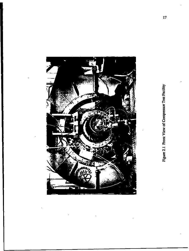
2.1 Front View of Compressor Test Facility ................................................ 17

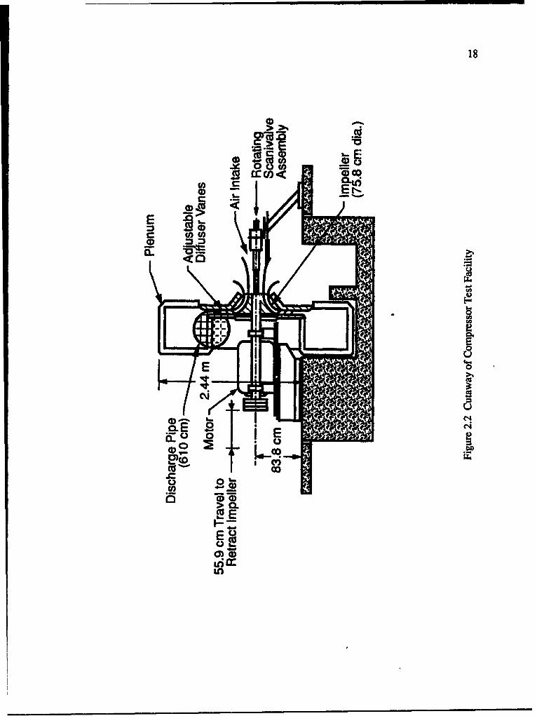
2 2 Cutaway of Compressor Test Facility .................................................. 18

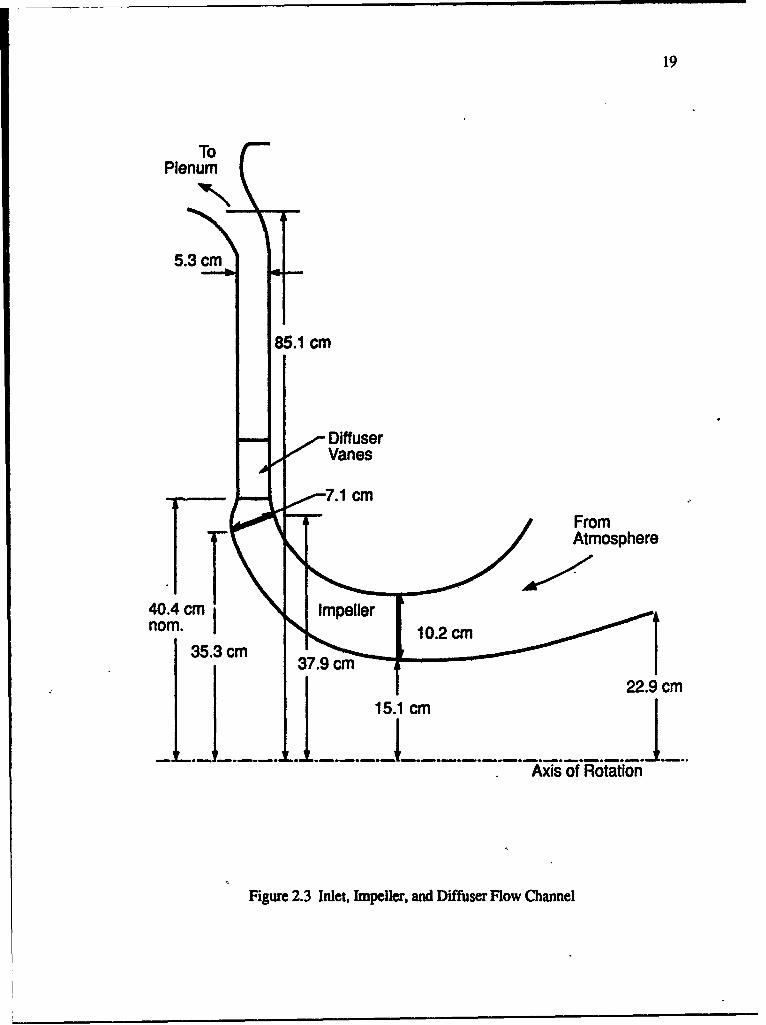
2.3 Inlet, Impeller, and Diffuser Flow Channel ............................................ 19

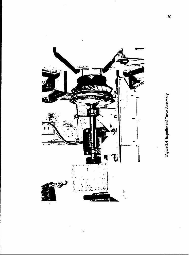
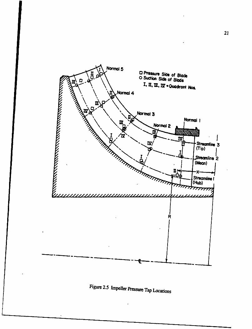
2.4 Impeller and Drive Assembly ............................................................ 202.5 Impeller Pressure Tap LocA ons ........................................................ 21

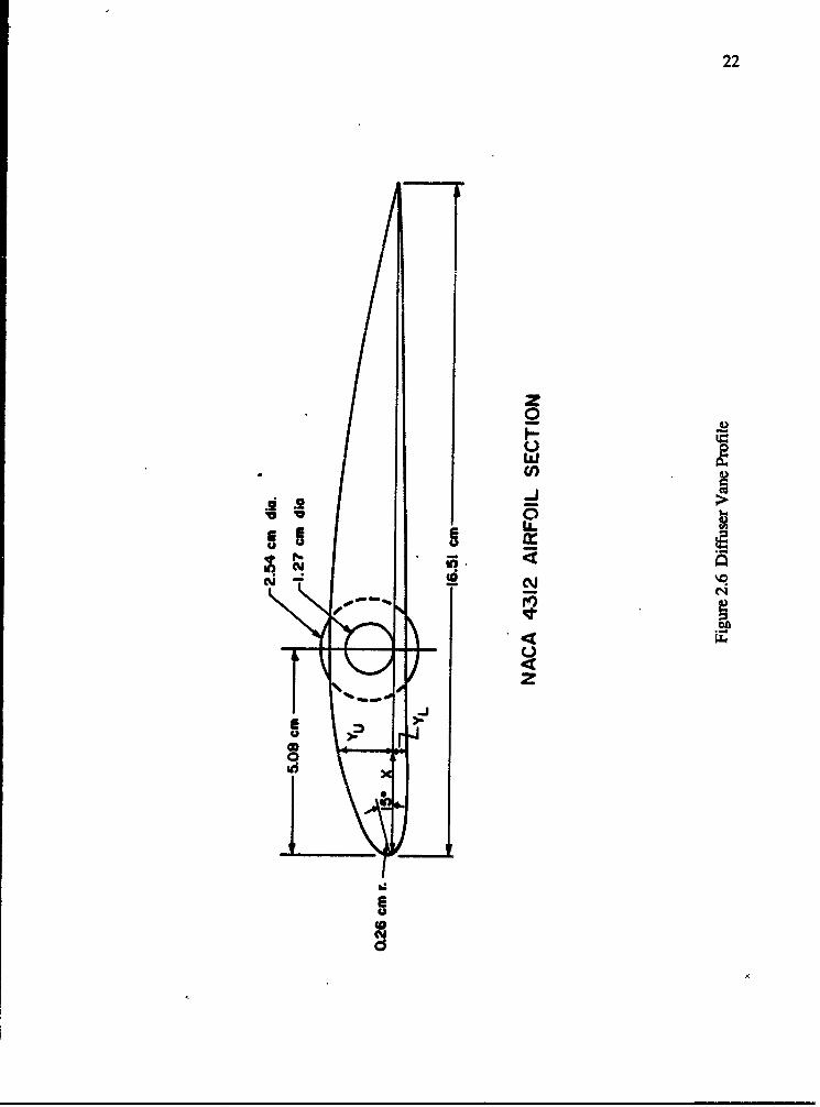
2.6 Diffuser Vane Profile ..................... ..................................... 22

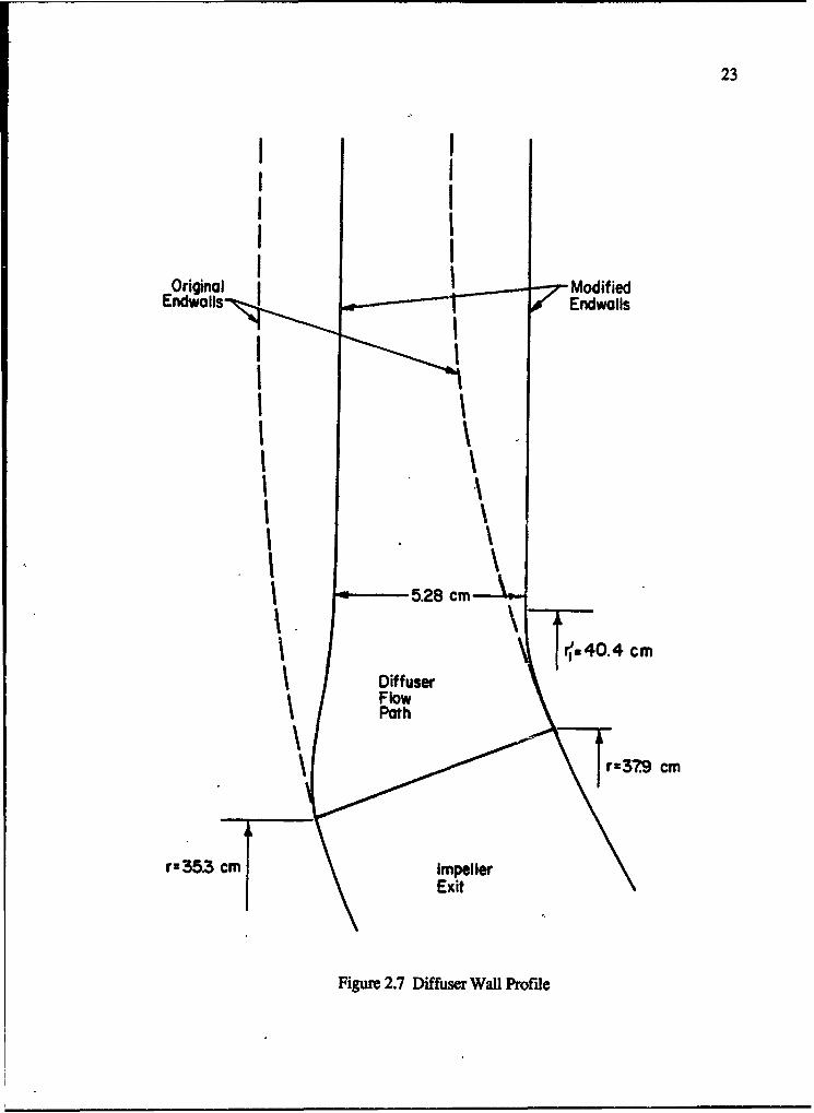
2.7 Diffuser Wall Profile .................................................................. 23

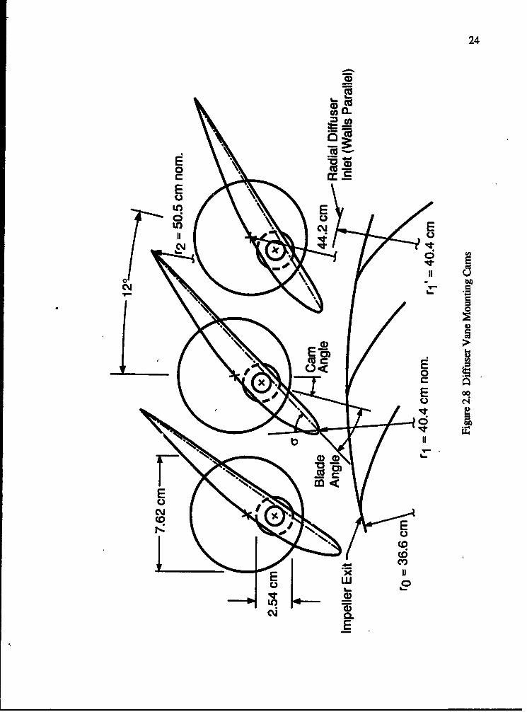
2.8 Diffuser Vane Mounting Cams .......................................................... 24

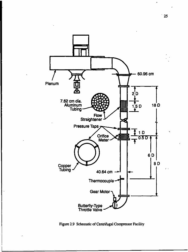
2.9 Schematic of Centrifugal Compressor Facility ........................................ 25

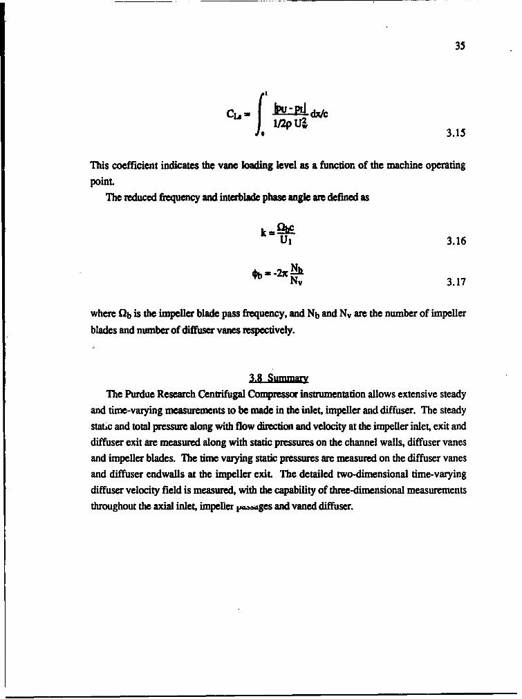
3.1 Rotating Scanivalve and LDV Final Optics ............................................ 36

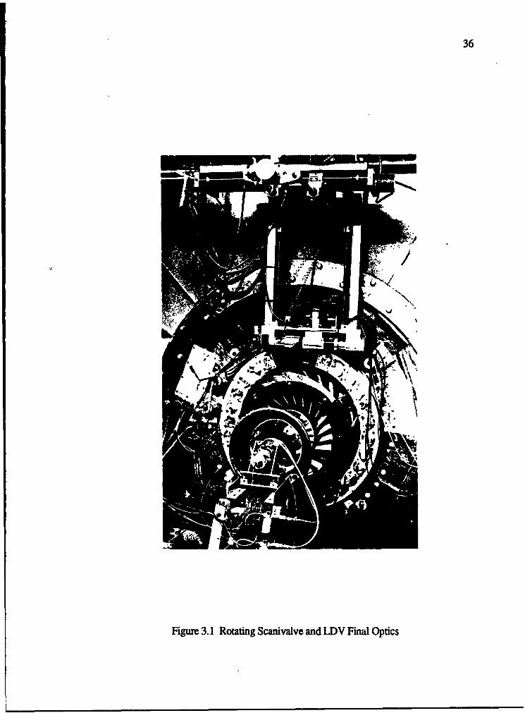
3.2 Pressure Probe Locations ................................................................ 37

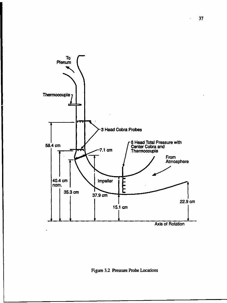
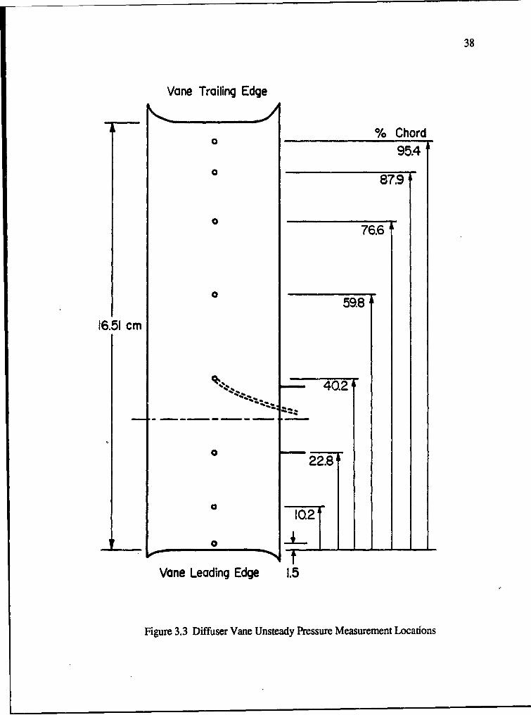
3.3 Diffuser Vane Unsteady Pressure Measurement Locations .......................... 38

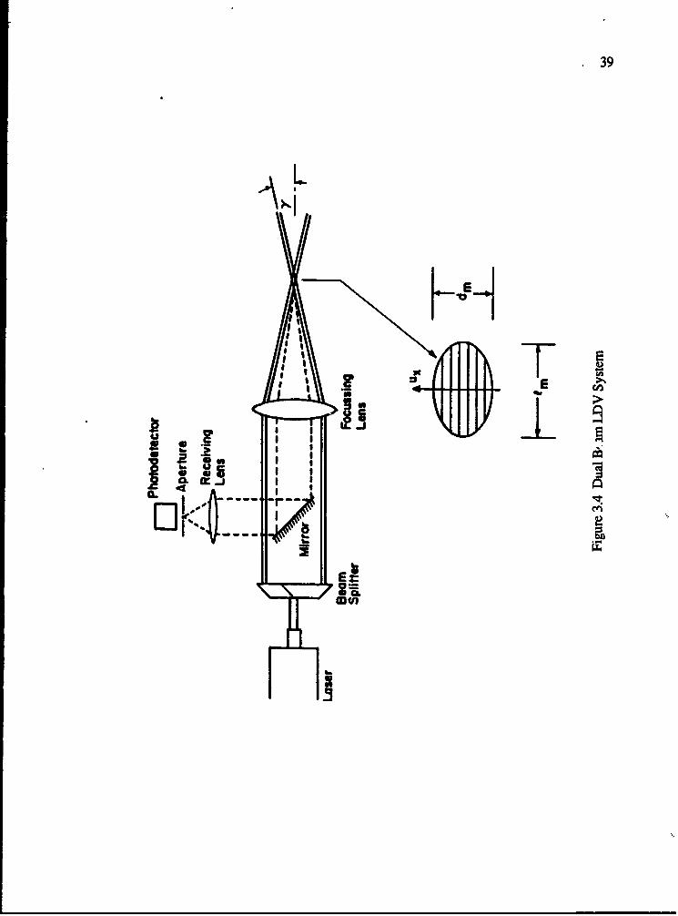
3.4 Dual Beam LDV Sy ,er .................................................................... 39

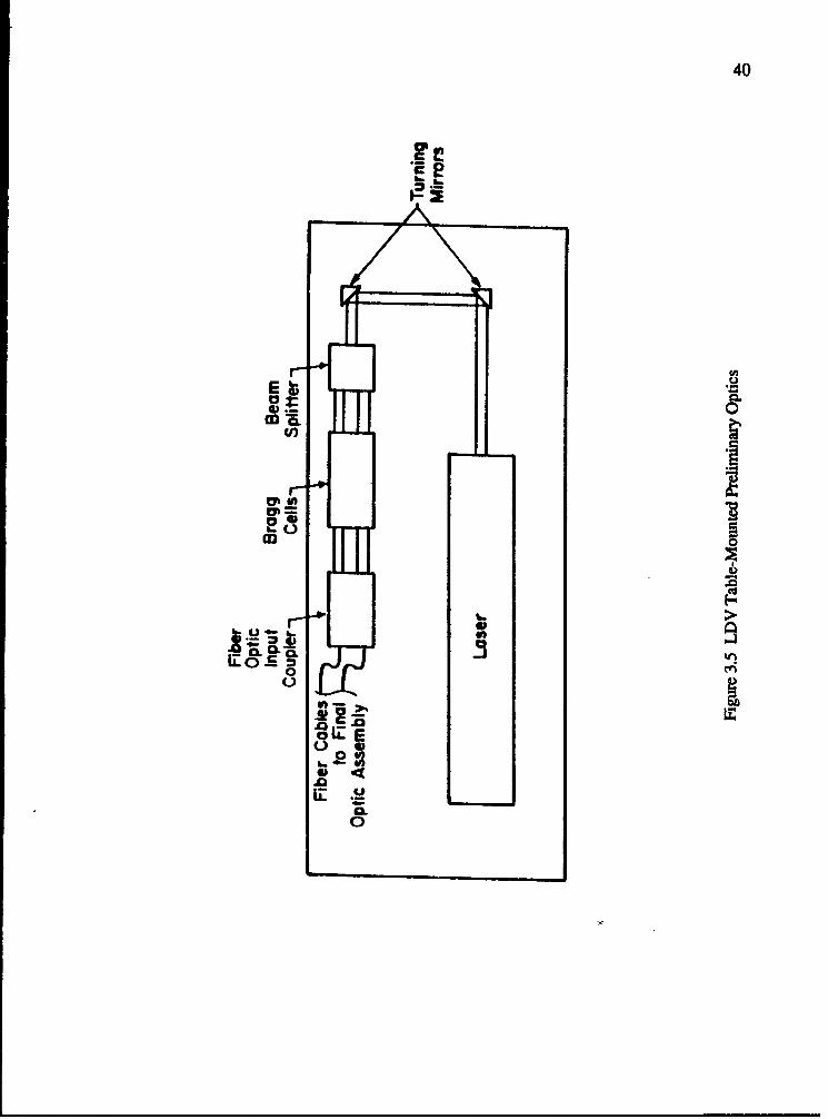
3.5 LDV Table-Mounted Preliminar Optics ............................................... 40

3.6 LDV Final Optics Assembly .............................................................. 41

4.1 Radial Turbomachine Wake ............................................................ 514.2 Radial Diffuser Unsteady Wake Velocity (oo = 60P, Nb = 12 and P0 = -450) ....... 52

4.3 Radial Diffuser Unsteady Wake Velocity (a0o = 450, Nb = 12 and 030 = -450) ....... 53

4.4 Radial Diffuser Unsteady Wake Velocity (a = 600 Nb = 12 and 3o = -30P) ....... 54

4.5 Radial Diffuser Unsteady Wake Velocity (oo = 60P, Nb = 12 and 3o = 0) ......... 55

4.6 Radial Diffuser Unsteady Wake Velocity (%0 = 600 Nb = 20 and f = -450) ....... 56

5.1 Radial Cascade Conformal Transformation ............................................ 68

5.2 Flat Plate Cascade Transformation ...................................................... 695.3 Translation and Torsion Upwash Transformation ..................................... 70

vii

Figure Page

5.4 Shed Vortical Gusts in Axial and Radial Turbonachines ............................. 71

5.5 Baseline Axial Flow Cascade Translational Lift ...................................... 72

5.6 Baseline Radial Flow Cascade Translational Lift ...................................... 73

5.7 Baseline Axia Flow Cascade Torsional Moment ..................................... 74

5.8 Baseline F adial Flow Cascade Torsional Moment .................................... 75

5.9 Baseline Axial Flow Cascade Convected Gust Lift ................................... 76

5.10 Baseline Radial Flow Cascade Convected Gust Lift ................................ 77

5.11 Radial Flow Cascade Translational Lift................................................. 78

5.12 Radial Flow Cascade Torsional Moment .............................................. 79

5.13 Radial Flow Cascade Convected Gust Lift ............................................ 80

5.14 Unsteady Airfoil Pressure for Translational Motion ................................... 81

5.15 Unsteady Airfoil Pressure for Torsional Motio ...................................... 82

5.16 Unsteady Airfoil Pressure for Convected Gust Upwash (k = 2.0) ................. 83

5.17 Unsteady Airfoil Pressure for Convected Gust Upwash (k = 4.0) ................. 84

6.1 Centrifugal Compwessor Performance with Vaneless Diffuser ......................... 102

6.2 Effect of Stagger on Compressor Performance (rl/ro = 1.10, Nv = 30) .............. 103

6.3 Effect of Stagger on Compressor Performance (rj/ro = 1.10, Nv = 15) ............ 104

6.4 Effect of Stagger on Compressor Performance (rj/ro = 1.15, Nv = 30) .............. 1056.5 Effect of Vane Number on Compressor Performance (ri/ro = 1.10, a = 500) ....... 106

6.6 Effect of Vane Number on Compressor Performance (rj/rO = 1.10, a = 600) ....... 107

6.7 Effect of Vane Number on Compressor Performance (rl/ro = 1.10, a = 700) ....... 108

6.8 Effect of Radius Ratio on Compressor Performance (a = 600, Nv = 30) ........ 109

6.9 Vaned Diffuser Nonuniform Circumferential Spacing Detuning ....................... 1106.10 Detuned Diffuser Compressor Performance (rl/ro = 1.10, a = 600, Nv = 30) ..... 1116.11 Detuned Diffuser Compressor Performance (rl/ro = 1.10, a = 600, Nv = 10) ..... 112

6.12 Impeller Static Pressure (Nv = 0, 0 = 0.17) ............................................ 113

6.13 Impeller Static Pressure (Nv = 0, 0 = 0.22) ............................................ 114

6.14 Impeller Static Pressure (Nv = 0, 0 = 0.30) ............................................ 115

6.15 Impeller Static Pressure (rf/ro = 1.10, w= 500, Nv = 30, 0 = 0.30) ................ 116

6.16 Impeller Static Pressure (rf/ro = 1.10, a = 600, Nv = 30, 0 = 0.22) ................ 117

6.17 Incidence Effects on Diffuser Vane Steady Static Pressure(ri/ro = 1.10, a = 600, Nv = 30) ....................................................... 118

vmi

Figure Page6.18 Vane Number Effects on Diffuser Vane Steady Static Pressure

(ri/ro = 1.10, a= 60 0, 0 =0.22) ...................................................... 119

6.19 Detuned Diffuser Vane Steady Static Pressure(ri/ro = 1.10, a = 60o, Nv - 30, 0 = 0.30) ............................. , ............ 120

6.20 IDV Measument Positios ............................................................. 1216.21 LDV Circumferential Measurement Bins ................................................ 1226.22 LDV Radial and Ccuin ntialMeasurement Positions ............................. 1236.23 Vaneless Diffuser Time-Averaged Velocity (0 - 0.30) ................................ 1246.24 Vaneless Diffuser Time-Averaged Velocity (0 = 0.22) ................................ 1256.25 Vaneless Diffuser Time-Averaged Velocity (0 = 0.17) ................................ 1266.26 Vaneless Diffuser Total Velocity (Tip Position, 0 = 0.30) ............................ 1276.27 Vaneless Diffuser Total Velocity (Mean Position, I =0.30) ......................... 1286.28 Vaneless Diffuser Total Velocity (Hub Position, 0 = 0.30) .......................... 1296.29 Vaneless Diffuser Total Velocity (Tip Position, 0 = 0.22) ............................ 1306.30 Vaneless Diffuser Total Velocity (Mean Position, 0 =0.22) ......................... 1316.31 Vaneless Diffuser Total Velocity (Hub Position, 0 = 0.22) .......................... 1326.32 Vaneless Diffuser Total Velocity (Tip Position, 0 = 0.17) ............................ 1336.33 Vaneless Diffuser Total Velocity (Mean Position, 0 ý-0.17) ......................... 1346.34 Vaneless Diffuser Total Velocity (Hub Position, 0 =0.17) .......................... 1356.35 Vaneless Diffuser Unsteady Velocity (Tip Position, 0 =0.30) ...................... 1366.36 Vaneless Diffuser Unsteady Velocity (Mean Position, 0 = 0.30) .................... 1376.37 Vaneless Diffuser Unsteady Velocity (Hub Position, 0 = 0.30) ..................... 1386.38 Vaneless Diffuser Unsteady Velocity (Tip Position, 0 = 0.22) ...................... 1396.39 Vaneless Diffuser Unsteady Velocity (Mean Position, 0=0.22) ..................... 1406.40 Vaneless Diffuser Unsteady Velocity (Hub Position, ( = 0.22) ..................... 1416.41 Vaneless Diffuser Unsteady Velocity (Tip Position, 0 =0.17) ...................... 1426.42 Vaneless Diffuser Unsteady Velocity (Mean Position, 0 = 0.17) .................... 1436.43 Vaneless Diffuser Unsteady Velocity (Hub Position, 0 = 0.17) ..................... 1446.44 Linear Theory Aerodynamic Gusts ....................................................... 1456.45 Vaneless Diffuser First Harmonic Unsteady V;eocity and Theory (0 = 0.30) ...... 1466.46 Vaneless Diffuser First Harmonic Unsteady Velocity and Theory (0 = 0.22) ...... 1476.47 Vaneless Diffuser First Harmonic Unsteady Velocity and Theory (0=-0.17) ...... 148

6.48 Vaneless Diffuser First Harmonic Unsteady Velocity and Theory(Theory O, = -160 0, 0 = 0.30) ......................... 1 o. o ... 149

ix

Figure Page6.49 Diffuser Vane First Harmonic Unsteady Lift (rl/ro = 1.10, Ny = 30) ............... 150

6.50 Diffuser Vane First Harmonic Unsteady Lift (rl/ro = 1.15, Nv = 30) ............... 151

6.51 Diffuser Vane First Harmonic Unsteady Lift (ri/ro = 1.10, Nv = 15) ............... 152

6.52 Diffuser Vane First Harmonic Unsteady Lift (rl/ro = 1.15, Nv - 15) ............... 153

6.53 Detuned Diffuser Vane First Harmonic Unsteady Lift (rl/ro = 1.10, Nv = 30) ..... 154

6.54 Detuned Diffuser Vane First Harmonic Unsteady Lift (rl/ro = 1.10, Nv = 10) ..... 1556.55 Diffuser Vane First Harmonic Unsteady Static Pressure

(rl/ro = 1.10, Nv = 30, a= 600, 0 = 0.30) .......................................... 156

6.56 Diffuser Vane First Harmonic Unsteady Static Pressure(ri/o = 1.10, Nv = 30, a= 600, 0 = 0.22) .......................................... 157

6.57 Diffuser Vane First Harmonic Unsteady Static Pressure(ri/ro = 1.10, Nv =30, a = 60 0, 0 = 0.17) .......................................... 158

6.58 Diffuser Vane First Harmonic Unsteady Static Pressure(Vane 1, 40% det., vl/ro = 1.10, Nv = 30, C = 600, 0 = 0.22) .................... 159

6.59 Diffuser Vane First Harmonic Unsteady Static Pressure(Vane 2, 40% det., rl/ro = 1.10, Nv = 30, ; = 60P, 0 = 0.22) .................... 160

6.60 Diffuser Vane First Harmonic Unsteady Static Pressure(rl/ro = 1.10, Nv = 15, a= 60o, 0 = 0.30) .......................................... 161

6.61 Diffuser Vane First Harmonic Unsteady Static Pressure(ril/ro = 1.10, Nv = 15, c = 600, 0 = 0.22) .......................................... 162

6.62 Diffuser Vane First Harmonic Unsteady Static Pressure(rjl/ro = 1.15, Nv = 15, a= 600, 0 = 0.30) .......................................... 163

6.63 Diffuser Vane First Harmonic Unsteady Static Pressure(ri/ro = 1.15, Nv = 15, a = 600, 0 = 0.22) .......................................... 164

6.64 Diffuser Vane First Harmonic Unsteady Static Pressure(rl/ro = 1.10, Nv = 10, a= 600, 0 =0.30) .......................................... 165

6.65 Diffuser Vane First Harmonic Unsteady Static Pressure(rl/ro = 1.10, Nv = 10, a = 600, 0 = 0.22) .......................................... 166

6.66 Rotating Stall Unsteady Static Pressure (Nv = 0, 0 = 0.155) ........................ 167

6.67 Rotating Stall Unsteady Static Pressure(rl/re = 1.10, Nv = 30, a = 60o, (b = 0.148) ......................................... 168

6.68 Rotating Stall Unsteady Static Pressure(rl/ro = 1.15, Nv = 30, a = 500, 0 = 0.160) ......................................... 169

x

IST OF SYMBOLS

Symbol Description

c Airfoil ChordCp Unsteady Pressure CoefficientCap Unsteady Pressure Difference CoefficientCL Unsteady Lift CoefficientCM Unsteady Moment CoefficientCO Steady Pressure CoefficientCAP Steady Pressure Difference Coefficient•L Steady Lift Coefficienth Translation Deflection

Steady Flow Incidencek Reduced Frequency, k=coc/U or coro/UNb Number of Impelle7 BladesNv Number of Diffuser Vanesp PressureP Steady Pressurer Radiusr Nondimensional Radius, r/ro or r/r1 'ro Impeller Exit Radiusrl Diffuser Vane Leading Edge Radiusr~l Radial Diffuser Inlet RadiusT2 Radial Vaned Diffuser Reference Radiuss Airfoil Circumferential Spacingt Nondimensional Time, t/(rolUo)u Streamwise VelocityU Unsteady Streamwise Axial VelocityU Steady Velocity

xi

Symbol Description

Ur Steady Radial VelocityUO Steady Tangential Velocity

uw Wheel Speedv Transverse Velocity

Vn Unsteady Transverse Velocity

Vr Unsteady Radial Velocityve Unsteady Tangential Velocityw Complex PotentialW Rotating Reference Frame Steady Velocityx Distant t Along Blade Chordz Radir" Cascade Complex CoordinateQL Logarithmic Spiral Angleao Impeller Exit Absolute Flow Anglea Pitching Deflection13o Impeller Exit Relative Flow AngleSwWake Velocity Vector Phase Angley LDV Half Angle

Axial Flow Cascade Complex CoordinateAxial Flow Cascade Axial Coordinate

0 Scaled Tangential Coordinate, 0/(U/Uw)

4 Axial Flow Cascade Tangential CoordinateP Densitya Diffuser Vane Stagger Angle

kb Interblade Phase AngleOw Wake Velocity Component Phase Angle0 Velocity Potential

Stream FunctionS'Pressure Rise CoefficientCO Frequency

Q Unsteady VorticityO Blade Passing Frequency

C4 Rotational Frequency

Steady Vorticity

CHAPTER 1

INTRODUCTION

Centrifugal compressors have found wide use in industrial, aerospace and groundbased transportation applications. Important systems include small gas turbine engine

compressors, piston engine turboclkgers, compressed air and refrigeration systems, and

turbopumps for liquid fueled rocket engines. The earliest jet engines employed centrifugal

compressors. However, axial compressors became favored due to their smaller crosssectional area which facilitated use in high-thrust jet engines. Centrifugal compressors do

have several distinct advantages, including their relative ease of manufacture and much

higher pressure rise per stage as compared with axial machines. These advantages have

begun to be exploited in the past two decades, prompting the need for research to improve

centrifugal compressor performance.

A centrifugal compressor is a rotating machine which increases the stagnation enthalpy

of a flowing fluid, with the throughflow mainly in a radial direction. It is this radialthroughflow which allows a centrifugal compressor to attain a very high pressure rise per

stage. The impeller and radial diffuser comprise a centrifugal compressor stage, with inletguide vanes sometimes utilized to impart prewhirl to the incoming flow. The radial diffuser

is generally vaneless. However, many modem compressor stages employ vaned diffusers

to increase efficiency.

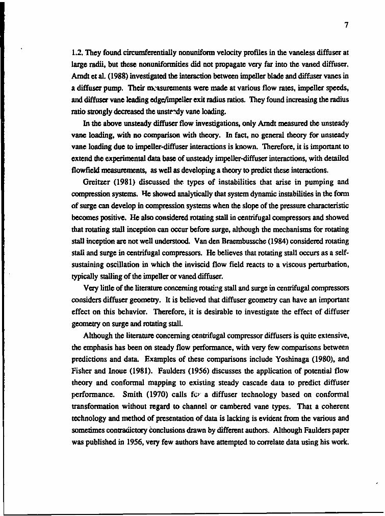
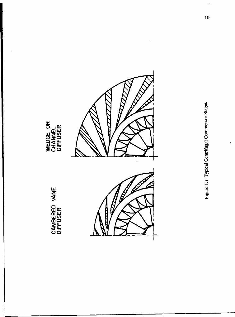
Two typical centrifugal compressor stages are depicted in Figure 1.1. The fluid enters

the impeller axially at the eye or inlet. Ideally, the forward portion of the impeller, termed

the inducer, allows the flow to enter the impeller smoothly and directs the flow radially.The fluid static pressure is continuously increased throughout the radial portion of the

impeller due to centripetal acceleration. A static pressure gradient exists across the impeller

channel resulting from the coriolis acceleration of the fluid. This gradient produces aýressure difference across each impeller blade which exerts torque on the impeller. The

flow leaving the impeller attains a greater velocity than the inlet flow due to the added wheelspeed. The radial diffuser is designed to receive this flow and to attain the largest possible

pressure recovery.

2

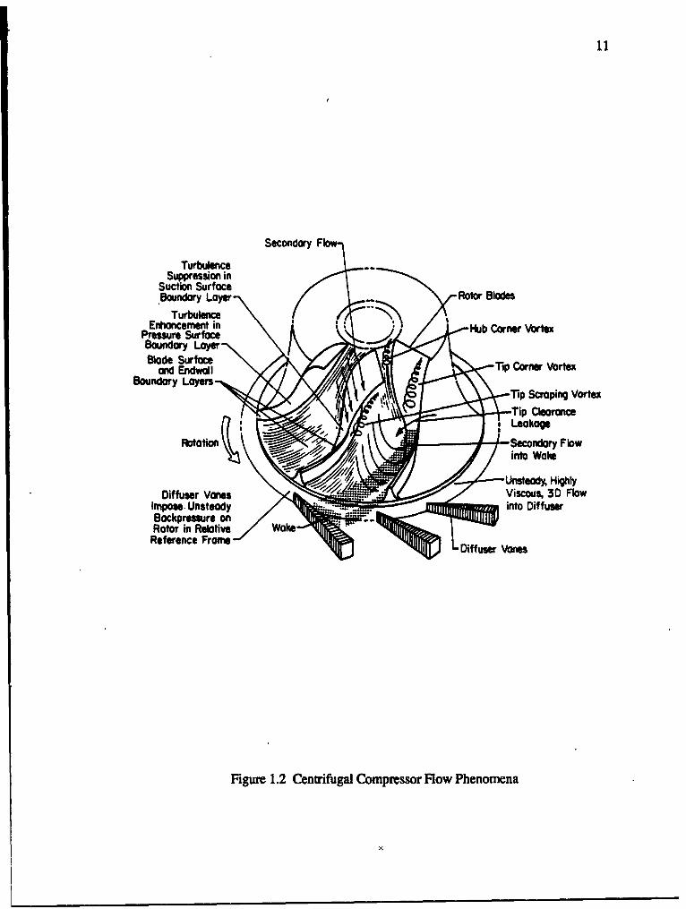
The actual flow through a centrifugal compressor stage is highly complex, as depictedschematically in Figure 1.2 (Wood, et al., 1983). The flow through the impeller passagesis complicated by several interacting phenomena. The static pressure and velocity arecircumferentially nonuniform at the impeller exit due to the potential effects of flow throughthe impeller passage and viscous effects manifested in trailing edge wakes and flowseparation. This circumferentially nonuniform flow is unsteady to the stationary diffuser,which is expected to attain the largest possible pressure recovery. The potential disturbanceof the diffuser vanes is also felt upstream, imposing an unsteady backpressure on therotating impeller. In addition to these periodic disturbances with the rotational or bladepassing frequency, instabilities can develop in centrifugal compression systems in the formof rotating stall and surge. All of these unsteady interactions and disturbances cansignificantly impact the compre=-or performance and produce aerodynamically inducedstress and vibration which may result in structural failure.

It has therefore become necessary to attain a greater understanding of the unsteady flowphenomena in centrifugal compressors. Since many modern centrifugal compressors

employ vaned diffusers, experimental investigations in conjunction with analyses areneeded to produce the most efficient designs and minimize undesirable unsteady flowphenomena.

1.1 oeration of Centrifugal Impgllers

The flow enters the forward portion of the impeller, which is termed the inducer. It isdesigned to allow the flow to enter the impeller smoothly and to turn the flow to a radialdirection with minimal loss. The inducer inlet blades are typically given some angle withrespect to axial to match the relative angle of the inlet flow over a certain range of operation.Most of the energy transfer to the air occurs in the radial portion of the impeller. Theblades at the impeller exit typically are radially oriented or given some angle from radialopposite the impeller rotation. The motivation for radially oriented blades includes ease ofmanufacture and reduced stress in high speed machines. Backswept blades are used tostabilize the impeller flow and reduce the velocity into the diffuser which aids in pressurerecovery. This lowers the power output of the stage but can increase the efficiency.Forward swept blades are rarely used.

In a centrifugal impeller, as previously mentioned, the flow in the impeller channel willbe nonuniform, producing a temporal variation in both the pressure and velocity at theimpeller exit. This causes the flow in the radial diffuser to be unsteady. In fact, Dean

3

(1959) shows that it is impossible for a turbomachine to work on a flowing fluid by otherthan viscous forces without time variation in the flow. It is therefore impossible for aturbomachine to operate without unsteady flow phenomena, with these phenomenagenerally inireasing in magnitude as the work output of the machine increases.

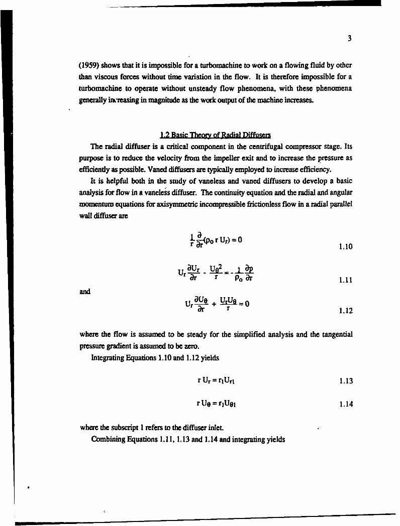
1.2 Basic Theory of Radial DiffusersThe radial diffuser is a critical component in the centrifugal compressor stage. Its

purpose is to reduce the velocity from the impeller exit and to increase the pressure asefficiently as possible. Vaned diffusers are typically employed to increase efficiency.

It is helpful both in the study of vaneless and vaned diffusers to develop a basicanalysis for flow in a vaneless diffuser. The continuity equation and the radial and angularmomentum equations for axisymmetric incompressible frictionless flow in a radial parallelwall diffuser are

a 4po r Ur) = 0r a1.10

Ur a ulr _U 2 - _or r Po ar 1.11

andUr -- 0 + r =-0r r 1.12

where the flow is assumed to be steady for the simplified analysis and the tangentialpressure gradient is assumed to be zero.

Integrating Equations 1.10 and 1.12 yields

r Ur = rjUrj 1.13

rUe = rjUoi 1.14

where the subscript I refers to the diffuser inlet.Combining Equations 1.11, 1.13 and 1.14 and integrating yields

4

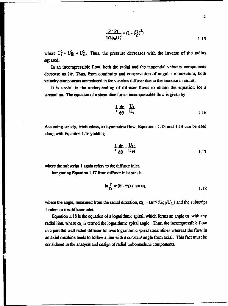
1/2poUr 1.15

where U2 = Uj, + U,21. Thus, the pressure decreases with the inverse of the radius

squared.In an incompressible flow, both the radial and the tangential velocity components

decrease as 1/r. Thus, from continuity and conservation of angular momentum, bothvelocity components are reduced in the vaneless diffuser due to the increase in radius.

It is useful in the understanding of diffuser flows to obtain the equation for a

streamline. The equation of a streamline for an incompressible flow is given by

I-& =r dO U0 1.16

Assuming steady, frictionless, axisymmetric flow, Equations 1.13 and 1.14 can be used

along with Equation 1.16 yielding

r dO U0I 1.17

where the subscript 1 again refers to the diffuser inlet

Integrating Equation 1.17 from diffuser inlet yields

In r = (0 - 01) tan aL=a 1.18

where the angle, measured from the radial direction, aL = tan'l(Uol/Uri) and the subscript

1 refers to the diffuser inlet.

Equation 1.18 is the equation of a logarithmic spiral, which forms an angle aL. with any

radial line, where a. is termed the logarithmic spiral angle. Thus, the incompressible flow

in a parallel wall radial diffuser follows logarithmic spiral streamlines whereas the flow in

an axial machine tends to follow a line with a constant angle from axial. This fact must be

considered in the analysis and design of radial turbomachine components.

5

1.3 Literature ReviewMuch attention in the literature has been given to centrifugal impeller and diffuser

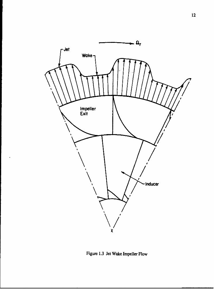
flowfields. The impeller exit flow, depicted in Figure 1.3, has typically been described asa jet-wake type of flowfield. Because of boundary layer growth and flow separation in theimpeller, the exit velocity profile is circumferentially nonuniform. This type ofcircumferentially nonuniform flow has been discussed by several authors. Dean and Senoo(1960) formulated a mathematical model of this jet-wake impeller flow. They concludedthat a reversible work interaction in circumferentially nonuniform flows between the jet andwake causes the velocity deficit to decrease rapidly within a small radial distance from theimpeller exit. They also discovered that the unsteady tangential velocity component in theradial diffuset can increase before its eventual decay. Eckardt (1975) performedmeasurements with high frequency instrumentation in the jet-wake flow of a low pressureratio centrifugal impeller. He found a significant jet-wake pattern existed and that the radialextension of the nonuniform circumferential velocity profile decayed more slowly thanpredicted by mathematical models such as the one formulated by Dean and Senoo.

Krain (1987) measured the velocity field within a newly designed impeller using anL2F system. Velocity profile nonuniformities were found within the impeller passages buta relatively uniform velocity profile at the impeller exit which differed significantly from thetypical jet wake pattern. Fagan and Fleeter (1989) measured the flowfield in the passagesof a mixed-flow, low pressure ratio centrifugal impeller. The traditional jet-wake exitflowfield pattern was observed at the design point and near stall. From theseinvestigations, it appears that although the typical impeller exit flow is nonuniformcircumferentially, the actual flow pattern is dependent on the impeller design, with evennear uniform profiles possible if separation in the impeller is controlled. The manyinteracting phenomena in impeller flows are not well understood, however, and it does notseem reasonable to expect either complete elimination of separation or circumferentiallynonuniform flows in radial impellers.

Vaned diffusers serve as flow guides and also incorporate turning of the flow so as toreduce the tangential velocity component at a greater rate than in a vaneless diffuser, thusreducing the size of the diffuser. Vaned diffusers have typically been of twoconfigurations: cambered vane diffusers and wedge or channel diffusers. Representativeexamples of these diffusers are shown in Figure 1.1. The cambered vane diffuser hasdeveloped from analogy to airfoil or turning vane cascades. Cambered vane diffusers withlogarithmic spiral profiles and little or no flow turning have been found to increase stage

6

efficiency (Smith, 1970). This is attributed to their ability to inhibit secondary flows and

separation. Thus, use uf vaned diffusers simply as flow guides can increase performance.The second major type of vaned diffuser is the wedge or channel diffuser. The purpose

of the channel diffuser is to remove the tangential velocity component and to limit the areaincrease of the diffuser. Channel diffusers are generally designed using some divergenceangle obtained from two-dimensional straight diffuser theory. Channel diffusers have beengiven much attention in the literature and have shown good performance.

Clements and Artt (1986) and Rodgers (1982) investigated the performance of channeltype diffusers considering the diffusion capabilities of different geometries. Clements andAnt conclude that the performance of channel diffusers is superior to that of cambered vanediffusers. Bammert, Jansen and Rautenberg (1983) considered both types of diffusersalong with a twisted vane diffuser. Their data does not support the conclusion of Clementsand Ant, with cambered vane diffuser stages having somewhat higher efficiency.Yoshinaga et al. (1980) investigated the performance of sixteen cambered vane diffuserswith moderate to high diffusion ratio. They compared their experimental results withpotential flow solutions using conformal mapping and found fair to good correlation withthe theory.

The effect of the radius ratio of the vaneless space in vaned radial diffusers has beendiscussed by several authors. Optimum values given range from 1.1 to 1.15 (Rodgers,1982; Bammert et al., 1983; Fisher and Inoue, 1981; Inoue and Cumpsty, 1984). It isgenerally concluded in the literature that vaned diffusers become less effective at largerradius ratios. Therefore, it is desired to position the diffuser vanes as close as possible tothe impeller while avoiding large unsteady interactions and reduced performance caused bythese interactions.

Very few investigations have considered the unsteady flow phenomena such as theinteractions between the impeller and the vaned diffuser or unsteady diffuser vane

performance. Fisher and Inoue (1981) made instantaneous measurements in the vanelessspace of a low speed compressor stage. However, only time averaged data were comparedto steady flow predictions from conformal mapping and Martensen singularity theory(Gostelow, 1984), with good correlation obtained. Although several authors haveconcluded that the vaned diffuser had little effect on the overall impeller performance,Fisher and Inouc concluded that the vaned diffuser significantly affects the impeller(." charge and vaneless space flowfield. Inoue and Cumpsty (1984) investigated impellerdischarge flow in vaneless and vaned diffusers. The vaned diffusers employed 10, 20 and30 blades and were operated at diffuser entrance/impeller tip radius ratios of 1.04, 1.1 and

7

1.2. They found circumferentially nonuniform velocity profiles in the vaneless diffuser at

large radii, but these nonuniformities did not propagate very far into the vaned diffuser.

Arndt et al. (1988) investigated the interaction between impeller blade and diffuser vanes in

a diffuser pump. Their measurements were made at various flow rates, impeller speeds,

and diffuser vane leading edge/impeller exit radius ratios. They found increasing the radius

ratio strongly decreased the unsteady vane loading.

In the above unsteady diffuser flow investigations, only Arndt measured the unsteady

vane loading, with no comparison with theory. In fact, no general theory for unsteadyvane loading due to impeller-diffuser interactions is known. Therefore, it is important to

extend the experimental data base of unsteady impeller-diffuser interactions, with detailedflowfield measurements, as well as developing a theory to predict these interactions.

Greitzer (1981) discussed the types of instabilities that arise in pumping and

compression systems. He showed analytically that system dynamic instabilities in the form

of surge can develop in compression systems when the slope of the pressure characteristic

becomes positive. He also considered rotating stall in centrifugal compressors and showed

that rotating stall inception can occur before surge, although the mechanisms for rotatingstall inception are not well understood. Van den Braembussche (1984) considered rotating

stall and surge in centrifugal compressors. He believes that rotating stall occurs as a self-

sustaining oscillation in which the inviscid flow field reacts to a viscous perturbation,typically stalling of the impeller or vaned diffuser.

Very little of the literature concerning rotatizig stall and surge in centrifugal compressors

considers diffuser geometry. It is believed that diffuser geometry can have an important

effect on this behavior. Therefore, it is desirable to investigate the effect of diffuser

geometry on surge and rotating stall.

Although the literature concerning centrifugal compressor diffusers is quite extensive,

the emphasis has been on steady flow performance, with very few comparisons betweenpredictions and data. Examples of these comparisons include Yoshinaga (1980), and

Fisher and Inoue (1981). Faulders (1956) discusses the application of potential flow

theory and conformal mapping to existing steady cascade data to predict diffuserperformance. Smith (1970) calls fer a diffuser technology based on conformal

transformation without regard to channel or cambered vane types. That a coherent

technology and method of presentation of data is lacking is evident from the various and

sometimes contradictory ýonclusions drawn by different authors. Although Faulders paper

was published in 1956, very few authors have attempted to correlate data using his work.

8

Much of the variation in the published dta is probably due to the dependence of the data on

the particular research facility.

Bryan and Fleeter (1987) experimentally investigated the effects of inlet prewhirl on the

impeller flowfield and overall performance of the Purdue Research Centrifugal

Compressor. This is a large scale, low speed machine which was originally designed and

operated by Vavra (1955). The facility was established at Purdue by Bryan and Fleeter and

is used in the current investigation. It was shown that inlet prewhirl significantly affected

the impeller flow, especially in the inducer region and that performance could be optimized

by varying inlet prewhirl. It was also discovered that very little effect of the prewhirl

propagated into the impeller discharge/diffuser region where the flowfield was almost

solely determined by flow rate.

Thus in summary, considerable effort has been made to determine the performance of

centrifugal compressor stages with emphasis on the radial diffuser. Investigations of

unsteady phenomena and the effect of diffuser geometry on such phenomena, however,

have bten given relatively little attention, with few or no theoretical predictions. Therefore,

it is imperative that these unsteady phenomena be investigated and the important machine

parameters affecting them be determined.

1.4 Research Objective and Technical Approach

The overall objective of this investigation is to quantify the dependence of significant

steady and unsteady flow phenomena inherent in centrifugal compressors on vaned diffuser

geometry, with emphasis on the radial vaned diffuser unsteady aerodynamics generated by

the impeller-diffuser interaction. Specific objectives include:

"• Determination of Centrifugal Compressor Performance

"* Impeller and Diffuser Vane Steady Loading Measurement

"* Diffuser Unsteady Flowfield Measurement

"• Diffuser Vane Unsteady Loading Measurement

"* Determination of Surge and Rotating Stall Occurrence and Characteristics

"* Development of Theory to Determine Radial Vaneless Diffuser

Wake Behavior -ind Unsteady Diffuser Vane Loading

The above experimental objectives were accomplished by performing a series of

experiments in the Purdue Centrifugal Compressor Facility. Steady flowfield

measurements were made using pressure probes throughout the machine to determine

9

performance. Steady surface static pressure measurements were made on the rotatingimpeller and vaned diffuser to determine loading. The time-variant flowfield in the radial

diffuser were measured using an LDV system. High response pressure transducers were

utilized to measure the unsteady diffuser vane surface static pressure as well as staticpressure variations at the impeller exit for determination of surge and rotating stall.

The above experiments were performed for various diffuser geometries and flow rates.

In particular, the number of diffuser vanes, the diffuser vane stagger, the diffuser vane

leading edge/impeller exit radius ratio and tCe circumferential spacing were varied

independently along with the mass flow rate through the machine. The compressor

performance and detailed flowfield were determined at each machine operating condition.Analyses were developed using linearized theory to predict the unsteady wake behavior

in the radial vaneless diffuser. This was incorporated into existing unsteady cascade theoryusing conformal mapping to predict the unsteady loading on the vaned diffuser due to

wakes shed from the rotating impeller.

10

cn

0 I0

wxCuciO

z

cruw(/

00

Secondary F

Suppression inSuction Surface

E~ancment nTiu Scrn ran Vortex

Precsure Surfaon

RefTenc Framenc

Figuree 1.2e Centrifuga CopDso Flwlheomn

12

-JetWake-

" ~Impeller/

II

\/

Exit

X

Figure 1.3 Jet Wake Impeller Flow

13

CHAPTER 2THE PURDUE RESEARCH CENTRIFUGAL COMPRESSOR

2-1 nemlThe Purdue Research Centrifugal'Compressor experimentally models the fundamental

aerodynamic phenomena inherent in centrifugal compressor stagc;s including thecircumferentially nonuniform impeller exit flow, diffuser vane incidence and radius ratio,and unsteady impeller diffuser interactions. The compressor is belt driven using a jackshaftand puiley arrangement by a 29.8 kW (40 hp) induction motor and is operated at 1790 rpm.The facility is shown in Figure 2.1 and depicted schematically in Figure 2.2.

The general operation of the machine can be described by considering the flow pathshown in Figure 2.3. Air is drawn into the machine through the bellmouth inlet sectionwhich converges to an axial direction at the impeller eye. The air enters the mixed flowimpeller which changes the axial inlet flow to a nearly radial flow at the outiet and alsoimparts a tangential component of velocity to the air. The center of the rotor is hollow,permitting the installation of instrumentation to transmit pressure data from the surfaces ofthe rotating blades to the data acquisition and analysis system located outside of themacnine in the stationary frame of reference.

On leaving the impeller, the air enters the radial diffuser whose walls curve smoothly toa parallel configuration. The air then passes through a row of stationary diffuser vaneswhich are located at the upstream portion of the parallel wall diffuser and is discharged intoa large annular plenum chamber. From this plenum, the air passes into a straight dischargepipe which contains a sharp edged orifice for flow rate measurement and a throttle valve toregulate the flow rate.

2. Impeller and Drive AssemblyThe impeller and drive assembly are shown in Figure 2.4. The impeller consists of 23

aluminum blades cast integrally with the hub. The tip is covered with a plexiglass shroudfor aerodynamic purposes and optical access. A mixed-flow impeller configuration is used

14

with a deloaded blade profile. In a mixed-flow impeller, the flow channels never turn to a

completely radial direction. Therefore, the flow maintains an appreciable component of

velocity in the axial direction during its entire passage through the impeller. With an

impeller of this type, the blade need not lie in a purely meridional plane, but may follow a

spiral path along the hub from inlet to exit. The use of a spiral type of flow path introduces

a great deal of flexibility into the aerodynamic design and permits use of a deloaded blade

design. In a general way, this is an impeller blade on which the pressure side is concave

over the first part of its length and essentially convex over the last part. This reversal of

curvature tends to reduce the aerodynamic loading near the blade exit and increase the

loading over the central portion of the blade.

The steady pressure distributions in the impeller blade passages are measured with

static pressure taps on the blade surfaces. There are 32 such taps, with two redundant

pairs, located along three streamlines at five normal locations. These are shown in Figure

2.5. The steady pressures on the impeller are measured using a rotating pressure

multiplexer.The shaft and motor are track mounted on a steel base. The entire impeller-drive

assembly can be retracted to perform necessary service. The impeller assembly utilizes

four cam mounted wheels which are lowered onto the track upon retracting the impeller.

When the impeller is in place, the wheels are raised allowing the base to rest in a v-groove

in the track. The base and impeller drive assembly are then bolted to the track. The

impeller is fixed in the stationary passages by a metal seal which bolts onto the rear passage

of the diffuser section downstream of the impeller. The inner part of this seal contains the

rear labyrinth seal.

The facility inlet allows air to flow smoothly from the atmosphere into the impeller.

The inlet tip wall consists of a plexiglass bellmouth of identical profile to the impeller bladetip. The inlet hub or centerbody consists of a conical section smoothly tapered to a cylinder

with a diameter equal to that of the impeller hub. The inlet has been developed using wall

tufts to detect separation points or flow nonuniformities. Pressure probe data show the

flow to be ye: y uniform at the impeller face.

15

2.4 Diffus~The radial diffuser consists of a smoothly curved vaneless space followed by a parallel

wall vaned radial diffuser. The diffuser vanes have a chord length of 16.5 cm (6.5 in.),with a NACA 4312 airfoil profile, Figure 2.6. The wall profile, Figure 2.7, facilitates theclose spacing of the diffuser vane leading edge and impeller trailing edge. This profile was

obtained by fitting a cubic spline from the impeller trailing edge to the parallel wall radial

diffuser. The performance of the diffuser flow path was evaluated by computing theaxisymmetric potential flow and applying the boundary layer code CBTSL with a Mangler

transformation, utilizing impeller exit flowfield data obtained by Fagan (1989) as aboundary condition. The flow in the diffuser was smooth and nonseparated over thedesign operating range, as indicated through flow visualization using wall tufts. Thediffuser tip wall contains 30 eccentric blade mounting cams, Figure 2.8, which allow thediffuser vane leading edge radius and stagger angle to be varied and also permitnonuniform circumferential vane spacing.

The diffuser walls are instrumented with a field of static pressure taps as well as statictaps along the diffuser vane chord at mid-span. A three head cobra probe is situated at theimpeller exit to measure total and static pressure as well as flow angle. Two similar probesare located downstream of the diffuser vane row.

2.5 Plenum and Exhaust PipingAn overhead schematic of the complete facility is shown in Figure 2.9. The diffuser

section is attached to the plenum into which the flow is discharged. The plenum is toroidalwith a square cross section. The inner diameter is 1.69 m (66.4 in.), the outer diameter is3.15 m (123.9 in.), and the width is 74.2 cm (29.2 in.). The plenum has a circular outletwith a 70.0 cm (24 in.) i.d. The exhaust piping system is attached to the plenum exit. Asair leaves the plenum, it enters a 900 elbow with an inner diameter of 70.0 cm (24.0 in.).The elbow is followed by a reducer which reduces the inner diameter to 40.6 cm (16 in.).A straight section of 40.6 cm (16 in.) inner diameter and 18 pipe diameters in lengthfollows the reducer. A flow straightener of 7.6 cm (3 in.) diameter tubing and 55.9 cm (22in.) length is lo-ated 2 pipe diameters downstream of the reducer to remove any swirling orradial nonuniformities in the flow. A sharp edged orifice plate of 30.48 cm (12.0 in.)orifice diameter in conjunction with 1-diameter and 1/2-diameter pressure taps is located atthe end of the straight section for mass flow measurement. A straight section 8 pipediameters in length is located behind the orifice plate and contains a thermocouple 6 pipe

16

diameters downstream of the orifice. A butterfly type throttle valve, driven by a gearmotor, is located at the exit of the 900 elbow to control the compressor flow rate. Themotor is actuated through a set of relays under control of the data acquisition system.

17

4-4-

0z

18

>

E F,,

C~CU

E (cc

uiU

CUO

19

ToPlenum

5.3 cm

85.1 cm

DiffuserVanes

, 7.1 cm"Fromy Atmosphere

40.4 cm Impellernom. 10.2 cm

15.1 cm 22.9 cm :S~22.9 cm

Axis of Rotation

Figure 2.3 Inlet, Impeller, and Diffuser Flow Channel

20

77)

21

11 1Norml 5 D P"Mresu Side of Blode0OSuclgon Side of Blade

Ilnral 4Ir3U~dGfl Not.

- - - ~ --t- -

Figue 25 Ipeler resur Ta3oain

22

z0

w

.44

z

> n4arUx

23

ErwlsEndwoll

5.8c

I 528 ccm

r=35.3 cm ImpellerExit

Figure 2.7 Diffuser Wall Profile

24

UlU

00

CDC

E c

25

60.96 cm

2 D

7.62 cm dfa.IAluminum ' D 8DTubing

FlowStraightener ,

Orifice -Meter 7 .

Tubing 40.64 cm-- -

Thermocouple

Gear Motor

Butterfly-Type IThrottle Valve

Figure 2.9 Schematic of Centrifugal Compressor Facility

26

CHAPTER 3DATA ACQUISTON AND ANALYSIS

In the current investigation, the data of fundamental interest are: 1) the compressor

steady operating conditions, including the aerodynamic performance of the impeller anddiffuser;, 2) the detailed impeller blade and diffuser vane steady aerodynamic loading

distributions, defined by the surface static pressure distributions; 3) the diffuser mean flow

field; 4) the impeller exit-diffuser vane inlet mean and periodic flow field; 5) the unsteady

pressure distributions on the diffuser vane surfaces; and 6) the unsteady static pressure at

the impeller exit/diffuser entrance.In this chapter, the instrumentation, data acquisition system and analysis techniques to

acquire these data are discussed. Static pressure taps (.n the impeller blades and diffuservanes and high response z.iniature pressure transducers embedded in the diffuser vanes

were used to determine the detailed steady and unsteady aerodynamic data. The diffuser

steady and time-variant flow field information was acquired with direction sensitive

pressure probes and laser Doppler velocimetery (LDV).

3.1 Steady Data Instrumentation

The centrifugal compressor steady data acquisition system is described in detail by

Bryan and Fleeter (1987). The time-averaged pressures on the stationary components are

measured using 6.9 kPa (1 psi) strain-gage pressure transducers in conjunction with aScanivalve pressure multiplexing system. The transducers are calibrated using a water

manometer with reference pressure and vacuum sources. The transducer output voltage ismeasured via computer using a Hewlett Packard HP3497 Data Acquisition Unit.

The impeller is instrumented with 32 static pressure taps on the rotating blade surfaces.The static pressures are measured using a rotating Scanivalve pressure multiplexer and

strain gage pressure transducer. The rotating Scanivalve multiplexer is capable of

measuring 36 static pressures on a rotating impeller. The Scanivalve employs a pneumatic

stepping motor and optical encoder.for positioning. The pressure from the rotating

27

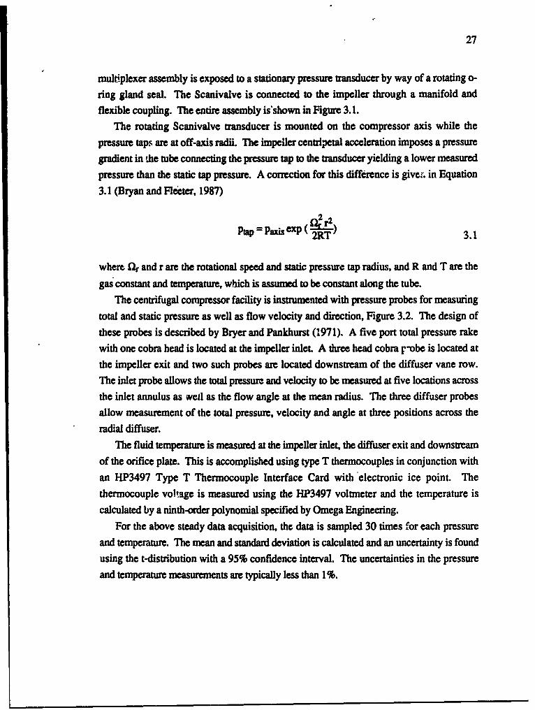
multiplexer assembly is exposed to a stationary pressure transducer by way of a rotating o-

ring gland seal. The Scanivalve is connected to the impeller through a manifold and

flexible coupling. The entire assembly is'shown in Figure 3.1.

The rotating Scanivalve transducer is mounted on the compressor axis while the

pressure taps are at off-axis radii. The impeller centripetal acceleration imposes a pressure

gradient in the tube connecting the pressure tap to the transducer yielding a lower measured

pressure than the static tap pressure. A correction for this difference is giver., in Equation

3.1 (Bryan and Fleeter, 1987)2

Ptap = Pais exp (2RT 3.1

where L1r and r are the rotational speed and static pressure tap radius, and R and T are the

gas constant and temperature, which is assumed to be constant along the tube.

The centrifugal compressor facility is instrumented with pressure probes for measuring

total and static pressure as well as flow velocity and direction, Figure 3.2. The design of

these probes is described by Bryer and Pankhurst (1971). A five port total pressure rakewith one cobra head is located at the impeller inlet. A three head cobra r-obe is located at

the impeller exit and two such probes are located downstream of the diffuser vane row.The inlet probe allows the total pressure and velocity to be measured at five locations across

the inlet annulus as wedl as the flow angle at the mean radius. The three diffuser probes

allow measurement of the total pressure, velocity and angle at three positions across the

radial diffuser.The fluid temperature is measured at the impeller inlet, the diffuser exit and downstream

of the orifice plate. This is accomplished using type T thermocouples in conjunction with

an HP3497 Type T Thermocouple Interface Card with electronic ice point. The

thermocouple voltage is measured using the HP3497 voltmeter and the temperature is

calculated by a ninth-order polynomial specified by Omega Engineering.For the above steady data acquisition, the data is sampled 30 times f.or each pressure

and temperature. The mean and standard deviation is calculated and an uncertainty is foundusing the t-distribution with a 95% confidence interval. The uncertainties in the pressureand temperature measurements are typically less than 1%.

28

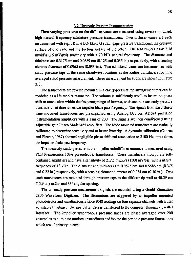
3.2 Unste dy Pressure Instrumentation

Time varying pressures on the diffuser vanes are measured using reverse mounted,

high natural frequency miniature pressure transducers. Two diffuser vanes are each

instrumented with eight Kulite LQ-125-5 G strain gage pressure transducers, the pressure

surface of one vane and the suction surface of the other. The transducers have 2.18

mv/kPa (15 mV/psi) sensitivity with a 70 kHz natural frequency. The diameter and

thickness are 0.3175 cm and 0.0889 cm (0.125 and 0.035 in.) respectively, with a sensing

element diameter of 0.0965 cm (0.038 in.). Two additional vanes are instrumented with

static pressure taps at the same chordwise locations as the Kulite transducers for time

averaged static pressure measurement. These measurement locations are shown in Figure

3.3.The transducers are reverse mounted in a cavity-pressure tap arrangement that can be

modeled as a Helmholtz resonator. The volume is sufficiently small to insure no phase

shift or attenuation within the frequency range of interest, with accurate unsteady pressure

transmission at three times the impeller blade pass frequency. The signals from the ,ffuservane mounted transducers are preamplified using Analog Devices' AD624 precision

instrumentation amplifiers with a gain of 200. The signals are then condi'ioned using

adjustable gain Ithaco Model 455 amplifiers. The blade mounted transducers are staticallycalibrated to determine sensitivity and to insure linearity. A dynamic calibration (Capece

and Fleeter, 1987) showed negligible phase shift and attenuation to 2100 Hz, three times

the impeller blade pass frequency.

The unsteady static pressure at the impeller exit/diffuser entrance is measured usingPCB Piezotronics 103A piezoelectric transducers. These transducers incorporate self-

contained amplifiers and have a sensitivity of 217.5 mv/kPa (1500 mV/psi) with a naturalfrequency of 13 kHz. The diameter and thickness are 0.9525 cm and 0.5588 cm (0.375

and 0.22 in.) respectively, with a sensing element diameter of 0.254 cm (0.10 in.). Two

such transducers are mounted through pressure taps to the diffuser tip wall at 40.39 cm

(15.9 in.) radius and 330 angular spacing.

The unsteady pressure measurement signals are recorded using a Gould Biomation2805 Waveform Digitizer. The Biomations are triggered by art impeller mounted

photodetector and simultaneously store 2048 readings on four separate channels with a user

adjustable timebase. The raw buffer data is transferred to the computer through a parallel

interface. The impeller synchronous pressure traces are phase averaged over 200

ensembles to eliminate random unsteadiness and isolate the periodic pressure fluctuations

which are of primary interest.

29

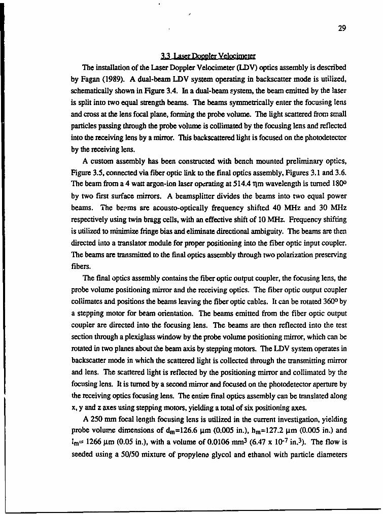
3.3 Laser Doppler Velocimeter

The installation of the Laser Doppler Velocimeter (LDV) optics assembly is described

by Fagan (1989). A dual-beam LDV system operating in backscatter mode is utilized,schematically shown in Figure 3.4. In a dual-beam system, the beam emitted by the laseris split into two equal strength beams. The beams symmetrically enter the focusing lensand cross at the lens focal plane, forming the probe volume. The light scattered from small

particles passing through the probe volume is collimated by the focusing lens and reflectedinto the receiving lens by a mirror. This backscattered light is focused on the photodetector

by the receiving lens.A custom assembly has been constructed with bench mounted preliminary optics,

Figure 3.5, connected via fiber optic link to the final optics assembly, Figures 3.1 and 3.6.The beam from a 4 watt argon-ion laser oprating at 514.4 ilm wavelength is turned 1800

by two first surface mirrors. A beamsplitter divides the beams into two equal powerbeams. The beams are acousto-optically frequency shifted 40 MHz and 30 MHzrespectively using twin bragg cells, with an effective shift of 10 MHz. Frequency shiftingis utilized to minimize fringe bias and eliminate directional ambiguity. The beams are then

directed into a translator module for proper positioning into the fiber optic input coupler.The beams are transmitted to the final optics assembly through two polarization preserving

fibers.The final optics assembly contains the fiber optic output coupler, the focusing lens, the

probe volume positioning mirror and the receiving optics. The fiber optic output coupler

collimates and positions the beams leaving the fiber optic cables. It can be rotated 3600 by

a stepping motor for beam orientation. The beams emitted from the fiber optic outputcoupler are directed into the focusing lens. The beams are then reflected into the test

section through a plexiglass window by the probe volume positioning mirror, which can berotated in two planes about the beam axis by stepping motors. The LDV system operates in

backscatter mode in which the scattered light is collected through the transmitting mirrorand lens. The scattered light is reflected by the positioning mirror and collimated by the

focusing lens. It is turned by a second mirror and focused on the photodetector aperture bythe receiving optics focusing lens. The entire final optics assembly can be translated alongx, y and z axes using stepping motors, yielding a total of six positioning axes.

A 250 mm focal length focusing lens is utilized in the current investigation, yieldingprobe volume dimensions of dm=126.6 gin (0.005 in.), hm=12 7.2 gm (0.005 in.) and

lm= 1266 gm (0.05 in.), with a volume of 0.0106 mm3 (6.47 x 10-7 in. 3). The flow isseeded using a 50/50 mixture of propyleno glycol and ethanol with particle diameters

30

between 0.5 and 1.5 jum. The velocity ratio for these particles at the impeller wheel speed,

Uw=80m/s, is greater than 98%.To determine the probe volume position and orientation, an inverse ray tracing

algorithm is used which performs an exact ray trace from the probe volume, through the

access window to the focusing lens. Prior to data acquisition, the six-axis positioning

system is manually positioned on a reference mark with proper orientation. The HP1000

computer initializes the stepper motor positioners, then the axis settings for the desired

measurement location and direction are used by the computer to move the six-axis

positioner to the desired location.A TSI Model 1990 Counter Processor is utilized for photodetector signal processing.

The Doppler burst frequency is determined from the time required for a seed particle tocross 16 probe volume fringes. Measurements with less than 16 fringe crossings areinvalidated. Along with the Doppler burst frequency time measurement, a 1 MHz clock

circuit is utilized to latch a timing word at the data ready signal from the counter processor

and is reset at each revolution. This timing word is transferred to the computer along with

the LDV word and ured to determine the impeller angular position at the instant of the

measurement. The 23 bladed impeller is divided into 460 circumferential bins, 20 per blade

passage, and the data is stored in the bin corresponding to the proper impeller position.Data is collected at a given location until a requisite number of samples are in each bin. Inthis scheme, the time varying velocity signal around the impeller circumference can bedetermined.

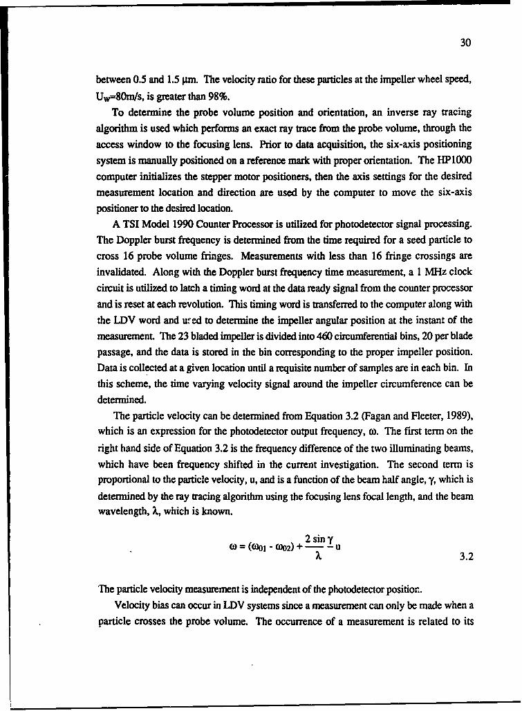
The particle velocity can be determined from Equation 3.2 (Fagan and Fleeter, 1989),which is an expression for the photodetector output frequency, (o. The first term on the

right hand side of Equation 3.2 is the frequency difference of the two illuminating beams,which have been frequency shifted in the current investigation. The second term isproportional to the particle velocity, u, and is a function of the beam half angle, y, which is

determined by the ray tracing algorithm using the focusing lens focal length, and the beam

wavelength, X, which is known.

0) = (0)01 (002) + 2 siny7X. 3.2

The particle velocity measurement is independent of the photodetector position.

Velocity bias can occur in LDV systems since a measurement can only be made when aparticle crosses the probe volume. The occurrence of a measurement is related to its

31

instantaneous velocity, since more particles will cross the probe volume in a given timeincrement at greater velocities. Roesler, Stevenson and Thompson (1980) discovered thatconstant frequency (equal time) sampling at lower frequency than the data realization rateeliminates the correlation between instantaneous velocity and sampling rate. Since the datain the current investigation are stored in bins according to impeller position, the data in eachbin is effectively equal time sampled and velocity bias is eliminated.

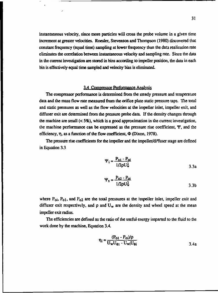
3.4 Comprssor Performance Analysis

The compressor performance is determined from the steady pressure and temperaturedata and the mass flow rate measured from the orifice plate static pressure taps. The totaland static pressures as well as the flow velocities at the impeller inlet, impeller exit, anddiffuser exit are determined from the pressure probe data. If the density changes throughthe machine are small (< 5%), which is a good approximation in the current investigation,the machine performance can be expressed as the pressure rise coefficient, ', and theefficiency, il, as a function of the flow coefficient, ID (Dixon, 1978).

The pressurie rise coefficients for the impeller and the impeller/diffuser stage are definedin Equation 3.3

-i = POp - Poi1t2pU2 3.3a

-s = P02 - Poi1/2pU2 3.3b

where Poi, P01, and Po2 are the total pressures at the impeller inlet, impeller exit anddiffuser exit respectively, and p and Uw are the density and wheel speed at the meanimpeller exit radius.

The efficiencies are defined as the ratio of the useful energy imparted to the fluid to thework done by the machine, Equation 3.4.

(PO - PoO/P1 UwUOl - UwjUoj 3.4a

32

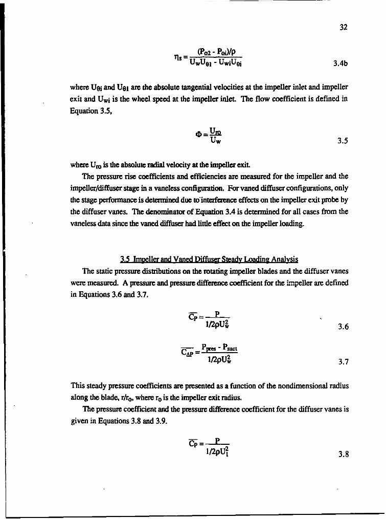
'Is = (Po2 - Po0 /P's=UwUot . UwiUei 3.4b

where Uoi and U61 are the absolute tangential velocities at the impeller inlet and impeller

exit and Uwi is the wheel speed at the impeller inlet. The flow coefficient is defined in

Equation 3.5,

Uw 3.5

where Uro is the absolute radial velocity at the impeller exit.The pressure rise coefficients and efficiencies are measured for the impeller and the

impeller/diffuser stage in a vaneless configuration. For vaned diffuser configurations, onlythe stage performance is determined due to interference effects on the impeller exit probe bythe diffuser vanes. The denominator of Equation 3.4 is determined for all cases from thevaneless data since the vaned diffuser had little effect on the impeller loading.

3.5 Imoeller and Vaned Diffuser Steady Loading Analysis

The static pressure distributions on the rotating impeller blades and the diffuser vaneswere measured. A pressure and pressure difference coefficient for the Li.peller are definedin Equations 3.6 and 3.7.

1/2pU~w 3.6

S- Ppes -suctl/2pUW2 3.7

This steady pressure coefficients are presented as a function of the nondimensional radiusalong the blade, r/ro, where ro is the impeller exit radius.

The pressure coefficient and the pressure difference coefficient for the diffuser vanes isgiven in Equations 3.8 and 3.9.

lI2pU 3.8

33

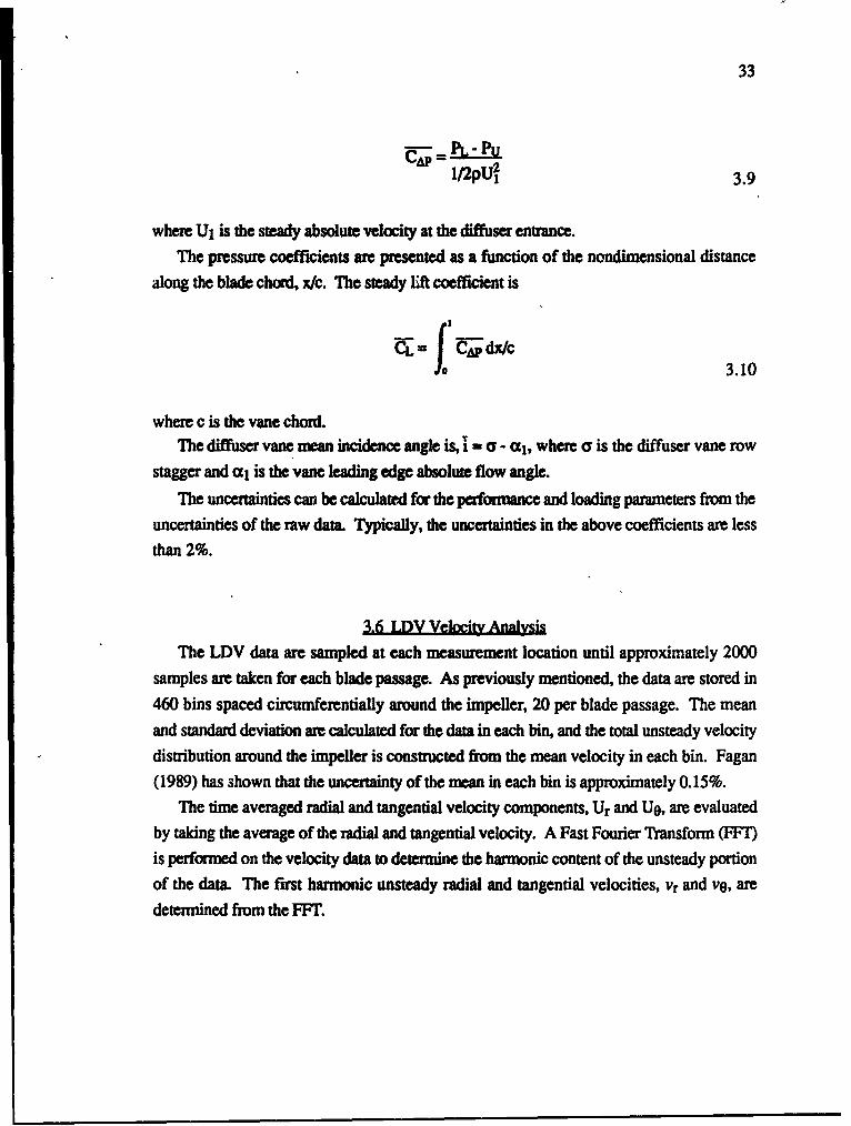
,=A1/2pU23.

3.9

where U1 is the steady absolute velocity at the diffuser entrance.The pressure coefficients are presented as a function of the nondimensional distance

long the blade chord, x/c. The steady Eft coefficient is

f ý dx/c 3.10

where c is the vane chord.The diffuser vane mean incidence angle is, I = a - cl, where a is the diffuser vane row

stagger and al is the vane leading edge absolute flow angle.

The uncertainties can be calculated for the performance and loading parameters from theuncertainties of the raw data. Typically, the uncertainties in the above coefficients are lessthan 2%.

3.6 LDV YeloCity AnalysisThe LDV data are sampled at each measurement location until approximately 2000

samples are taken for each blade passage. As previously mentioned, the data are stored in460 bins spaced circumferentially around the impeller, 20 per blade passage. The meanand standard deviation are calculated for the data in each bin, and the total unsteady velocitydistribution around the impeller is constructed from the mean velocity in each bin. Fagan(1989) has shown that the uncertainty of the mean in each bin is approximately 0.15%.

The time averaged radial and tangential velocity components, Ur and U0, are evaluatedby taking the average of the radial and tangential velocity. A Fast Fourier Transform (FFT)is performed on the velocity data to determine the harmonic content of the unsteady portionof the data. The first harmonic unsteady radial and tangential velocities, vr and ve, aredetermined from the FFr.

34

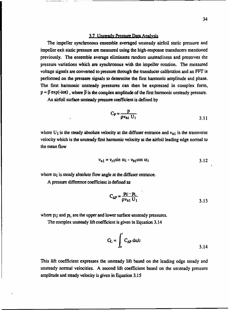
3.7 Unsteady Pressure Data AnalysisThe impeller synchronous ensemble averaged unsteady airfoil static pressure and

impeller exit static pressure are measured using the high-response transducers mentionedpreviously. The ensemble average eliminates random unsteadiness and preserves thepressure variations which are synchronous with the impeller rotation. The measuredvoltage signals are converted to pressure through the transducer calibration and an FFT isperformed on the pressure signals to determine the first harmonic amplitude and phase.The first harmonic unsteady pressures can then be expressed in complex form,p = i exp(-iwOt) , where P is the complex amplitude of the first harmonic unsteady pressure.

An airfoil surface unsteady pressure coefficient is defined by

Cp = Ppvn U1 3.11

where U1 is the steady absolute velocity at the diffuser entrance and Vnl is the transversevelocity which is the unsteady first harmonic velocity at the airfoil leading edge normal to

the mean flow

vnj = vrlsin ot, - ve1cos a, 3.12

where ocl is steady absolute flow angle at the diffuser entrance.

A pressure difference coefficient is defined as

Cap = PU - PPVni Ui 3.13

where Pu and PL are the upper and lower surface unsteady pressures.The complex unsteady lift coefficient is given in Equation 3.141'

CL = CAp dx/c3.14

This lift coefficient expresses the unsteady lift based on the leading edge steady and

unsteady normal velocities. A second lift coefficient based on the unsteady pressureamplitude and steady velocity is given in Equation 3.15

35

CLU IJV2p Uw2 3.15

This coefficient indicates the vane loading level as a function of the machine operatingpoint.

The reduced fiequency and interblade phase angle are defined as

U1 3.16

2Nv 3.17

where Ob is the impeller blade pass frequency, and Nb and Nv are the number of impeller

blades and number of diffuser vanes respectively.

The Purdue Research Centrifugal Compressor instrumentation allows extensive steady

and time-varying measurements to be made in the inlet, impeller and diffuser. The steady

static and total pressure along with flow direction and velocity at the impeller inlet, exit and

diffuser exit are measured along with static pressures on the channel walls, diffuser vanes

and impeller blades. The time varying static pressures are measured on the diffuser vanes

and diffuser endwalls at the impeller exit. The detailed two-dimensional time-varying

diffuser velocity field is measured, with the capability of three-dimensional measurements

throughout the axial inlet, impeller paa•ges and vaned diffuser.

36

Figure 3.1 Rotating Scanivalve and LDV Final Optics

37

TOPlenum

n mThermocouple

3 Head Cobra Probes

5 Head Total Pressure with58.4 cm Center Cobra and7.1 cm ThermocoupleS~From

40.4 cm mpellernom.

35.3 cmi

15.1 cm

Axis of Rotation

Figure 3.2 Pressure Probe Locations

38

Vane Trailing Edge

% Chord0

95.4

87.9A

0

76.6

0 59.8

16.51 cm

40.2

0 22.8

10.2

Vane Leading Edge 1.5

Figure 3.3 Diffuser Vane Unsteady Pressure Measurement Locations

39

COLLFl i

40

E c2oU)

bC.)200

CaCu

1) C

0

41

S Cc0IS

I I

B'A

% SI

% %

% % 1"- , - i. - -

-I

-- "'

42

CHAPTER 4

RADIAL DIFFUSER WAKE ANALYSIS

Several analyses have been developed to predict the unsteady pressure distribution on

axial flow cascades (Whitehead, 1960; Whitehead 1978; Chiang and Fleeter, 1988) andrecently in radial flow cascades (Bryan and Fleeter, 1990). Typically, these unsteady

aerodynamic models are linearized, i.e., the unsteady velocities and pressures are

considered small perturbations superimposed on a steady mean flow, with second order

and higher terms neglected. The unsteady velocity field is predicted by solving for the

unsteady velocity potential, with boundary conditions given far from the blade row andalso on the blade surface. When solving for the unsteady pressure distribution generatedby an upstream wake, the velocity induced by the wake on the airfoil surface is specified as

a boundary condition. In most models, the wake is assumed to be convected through thecascade, undisturbed by the airfoils. Only the effect of the wake on the airfoil unsteady

pressure distribution is considered.

In this chapter, a mathematical model is developed to determine the behavior of vortical

wakes in a radial vaneless diffuser for use in unsteady aerodynamic models for radial flow

blade rows. Several investigations have considered both steady and time-variant radial

diffuser flows, including unsteady wake behavior (Dean and Senoo, 1960; Senoo andIshida, 1975). These unsteady wake models are control volume solutions and are not

directly applicable for use as boundary conditions in unsteady airfoil models. Therefore, amodel is developed which describes the behavior of small amplitude vortical impeller

wakes convected through the ridial diffuser by the mean flow.

4.1 Analysis

The flowfield in a parallel wall radial.vaneless diffuser is considered. The flow in theradial diffuser is assumed to be incompressible and inviscid. The imposed boundary

conditions are derived from the flow behind a radial impeller, with these boundary

43

conditions assumed to be equal to the radial diffuser inlet boundary conditions where

velocity measurements are made.

The radial and tangential velocities are considered to consist of a small amplitude

unsteady velocity superimposed on the mean steady velocity.

Vr = Ur + Vr 4.la

vo = U(0 + vo 4.1b

The nonuniform circumferential flow leaving the relative reference frame of the centrifugal

impeller is unsteady in the absolute reference frame of the radial diffuser, Figure 4.1.

Since the flow is inviscid, the flowfield can be described using the unsteady Eulerequations. Assuming the unsteady flow to be a small disturbance superimposed on thesteady mean flow, Equations 4.1, the steady and unsteady velocities can be described byseparate equations, where second order terms in the unsteady velocities are neglected.

(V-V) as = 0 4.2a

2V _Vs=-s 4.2b

Cit 4.3a

V2 4.3b

where V is the steady velocity vector, Q and !s are the unsteady and steady vorticity and V

and Vs are the unsteady and steady stream functions. The steady flow, Equations 4.2, is

independent of the unsteady flow, however, the unsteady flow, Equations 4.3, is

dependent on the steady flow.The boundary conditions for Equations 4.2 and 4.3 in the relative reference frame of

the impeller are depicted in Figure 4.1 and given by Equations 4.4.

vr = Wo cos 13o + vro exp (i Nb Or) @ r=ro 4.4a

44

ve = Wo sin 3o + voo exp (i Nb Or) @ r=ro 4.4b

VrV=O as r--)oo 4.4c

where Wo is the mean velocity in rotating frame, Nb is the number of impeller blades, P3o is

the mean relative flow angle, ro is the impeller exit radius and vro and vo0 are the complex

amplitudes of the wake velocities at the impeller exit.

The boundary conditions specified in Equations 4.4 can be transformed to the

stationary reference frame by adding the wheel speed Uw to the tangential velocity andexpressing the relative tangential coordinate, Or, in terms of the absolute tangential

coordinate 0, and time, t. The absolute coordinate 0, is related to the relative coordinate Or,

by 0 = Or + ot. Substituting this into Equations 4.4 and adding the wheel speed yields the

radial and tangential velocity boundary conditions at the impeller exit.

vr = Wo cos 3o + vro exp (ik(O- t)) @ r = ro 4.5a

ve=Wosinio+V0oexp(ik(0-t))+Uw @r=ro 4.5b

where 0 = O/(U/Uw) and t is scaled by ro/Uo, where U0 is the steady absolute velocity at

the impeller exit.The solution to Equations 4.2, assuming no variation in the steady velocity with 0, are

Ur=Uro/r 4.6a

U6 =U90/r 4.6b

where Uro and U0o are the steady mean absolute velocities at the impeller exit radius, ro,

and r is the nondimensional radius, r/ro.

The unsteady vorticity equation, Equation 4.2a, in radial coordina.•:s is

+ - r a + 9a+ r 50+ =07. a r4.)

45

With Ur and U0 determined, Equation 4.7 can be solved for the unsteady vorticity, 91. The

unsteady vorticity is considered an harmonic function of time,

= fl exp (-i 0) t) 4.8

where f is the complex unsteady vorticity amplitude which is a function of r and 0.Substituting Equations 4.4 and 4.8 into Equation 4.7 yields the following equation for

the unsteady vorticity amplitude, •.

r r2 TO0 4.9

where Uro and U0o are nondimensionalized by the absolute velocity leaving the impeller,Uo, and k is the reduced frequency, owo/Uo.

Equation 4.9 is a first order, linear partial differential equation with the followingsolution (Zachmanoglou and Thoe, 1986)

= CIO exp(2- i r2) f(r exp(- 0)) 4.10

where CIO is the complex amplitude of the unsteady vorticity and f is a functional form to be

determined.

The functional form, f, can be determined from the boundary conditions, Equations

4.5. The vorticity is defined as

a -L 2(rveo___av.r ar ra, 4.11

Since Ql is determined from partial derivatives of the velocity, the dependence of KI on 0must be the same as the dependence of the velocity derivatives, which is an exponential.

Therefore, the functional form, f, must be

f(x) = x (-iNb(Ueo/Ur,)) 4.12

The unsteady vorticity, determined from Equation 4.8, becomes,

46

J=1 foexp(A In r + B r2) exp(ik0 ) 4.13

where

A =-ik! O= --ik tan ao and B- ik _ ik,UwUro (tana- t an 30 ) cos ao 2 U-. 2 cos co

and ao is the steady mean flow angle in the absolute coordinate system.To determine the unsteady stream function, V, the expression for the unsteady

vorticity, Equation 4.13, is substituted into Equation 4.3b.

_L rr: . .U. .2 DO- exp(A In r + B r2) exp(ik 0 4.14ar2 r ar r2 a~ 8241

The solution to Equation 4.14 is determined as a complex Fourier series by a finite Fouriertransform, Equation 4.15, taking advantage of the fact that the solution is periodic in 0.

W(r,O)= • cn(r) eino 4.15n -=

The left hand side coefficients are defined by

(ic•./n

cn(r) =-a 2 l (rO) e'indO 4.16

and the source term coefficients are

C _(r) n Q(r,O) einO dO2 n 4.17

47

Substituting Equations 4.16 and 4.17 into Equation 4.14 yields

d2 cn +_Ld--A- k2 IU_ Cn = -r0 2 2oexp(A In r + B r 2) 4.18dr2 r dr r2 kUw I

Equation 4.18 is a Cauchy-Euler differential equation. The complementary solution is

given in Equation 4.19 (Ross, 1980).

cn = a rk2 + a2 r'k2 4.19

where k2 = k(Uo/Uw).

The particular solution to Equation 4.19 is found by variation of parameters. The

complete solution for cn is given in Equations 4.20 and 4.2 1.

Cn = al rk2 + a2 r-k2 + r202 Qrk2 exp(A In r + Br 2) r I - k2 dr2k 2 jj

.r 02 p r-k2 I exp(A In r + B r 2) rl + k2 dr 4.202k 2 f

and c-n = b rk2 + b2 r'k2 4.21

The stream function can be constructed from the Fourier series, Equation 4.15.

r02 10 ork2 exp(A In r + Br2) rl - k2 dr -2 2k2 f

r-k2 j exp(A In r + B r 2) rI + k2 dr exp(ik(O - t)) +

(al rk2 + a2 r-k2) exp(ik(O - t )) + (b1 rk2 + b2 rk2) exp(ik(-O - t)) 4.22

48

Since the solution is not a function of e"ikO bI and b2 are zero. The unsteady radial and

tangential velocities are evaluated from the stream function.-V i=.I 0__ = r % rk2-1I exp(AIn r +Br2) rl -k2 dr.

Vr r a 2

r-k2- 1 exp(A in r + B r 2) rI + k2 dr exp(ik(9 - t)) +

jikai rk2. I + *a.a r-k2. 1)exp(ik(O. t)) 4.23

and

-IV0 "- "2- IA exp(A In r + Br 2) rl - k2 dr +

r-k2- If exp(A In r + B r 2) rI + k2 dr exp(ik(0 - t)) +

kU lA2-I, k~rk 2 +~~r-k2 -1)~ exp(ik(9 - t) 4.24ro ro

The unsteady wake velocities, Equations 4.23 and 4.24, are composed of a vortical

velocity component and an irrotational velocity component. The irrrotational component

corresponds to the homogeneous solution of Equation 4.14, with the rotational componentcorresponding to the particular solution, which contains the 00 term in Equations 4.23 and

4.24.

The unsteady wake velocity solution, Equations 4.23 and 4.24, is determined by

specifying ao, 13o and k. The integrals are evaluated numerically using Simpson's 1/3

rule. The constants al and a2 are evaluated from the boundary conditions, Equations 4.5aand 4.5b. The vorticity magnitude, o20, is evaluated from the third boundary condition,

Equation 4.4c.

The unsteady wake velocities, Vr and vy, are for a vaneless, parallel wall, radial

diffuser. The steady flowfield is determined by the absolute flow angle, .0o. The wake

49

propagation is determined by the relative flow angle, P3o, the reduced frequency, k, and theboundary conditions of the wake, Vr0 and vo0 . In principle, the wave number, k2, can

assume any value for given ao, P3o and k. In practice, k2 is equal to the number of impeller

blades, Nb, and will always be an integer. Thus, given the number of impeller blades, Nb,

the relative flow angle, Po, and the absolute flow angle, ao, the unsteady wake velocities

can be determined from Equations 4.23 and 4.24.

The unsteady wake model developed herein is utilized to demonstrate the effect ofsteady centrifugal compressor parameters, including the absolute flow angle, c0o, the

relative flow angle, 03o, and the number of impeller blades, Nb. The unsteady wake

velocities, Vr and v0, are constant amplitude harmonic functions of the tangential coordinate

0, -id time t, at a particular value of r. However, the velocity varies in amplitude with r

due to the radial geometry and thus variation in steady velocity with radius. In the

following figures, the radial dependence of Vr i v0 is presented as a function of the

nondimensional radius, assuming no variation of the relative flow angle, 03o, with the

tangential direction, 0. A parametric study is performed by varying a0, 13o and Nb. The

baseline values are ao = 600, Nb = 12 and 0o = -450. Negative J0 values indicate impeller

blades leaning in the opposite direction of rotation.Figures 4.2 and 4.3 show the results for the baseline case with aOo = 600 and for

ao = 450. The radial velocity monotonically approaches zero whereas the circumferential

velocity increases to a maximum before approaching zero. This behavior is typical for

00 < -450. The radial velocity decreases more rapidly than the tangential velocity, with

both components decreasing more rapidly as the absolute flow angle, ao is increased.

Figures 4.4 and 4.5 show the wake velocities for 0o = -30o and J3o = 00. Changing

P3o, the relative flow angle, changes the boundary conditions for vro and V0o, under the

assumption of circumferentially constant 00. For various values of 030, the radial velocity

component demonstrates behavior similar to the baseline, with only a magnitude variation.

The tangential velocity again increases before its eventual decay, but the maximum occurs

at larger values of r for I0o closer to zero.

Figure 4.6 presents the wake velocities with Nb = 20. Variation in the number of

impeller blades, Nb, has a minimal affect on the amplitude of the wake velocities, with only

the phase changing more rapidly with increasing Nb.

50

The predicted wake velocities, Vr and vO, will be compared to the measured wakevelocities in the vaneless radial diffuser configuration of the Purdue Research Centrifugal

Compressor. As mentioned previously, these velocity expressions will also be utilized as aboundary condition in the unsteady radial airfoil cascade analysis in Chapter 5.

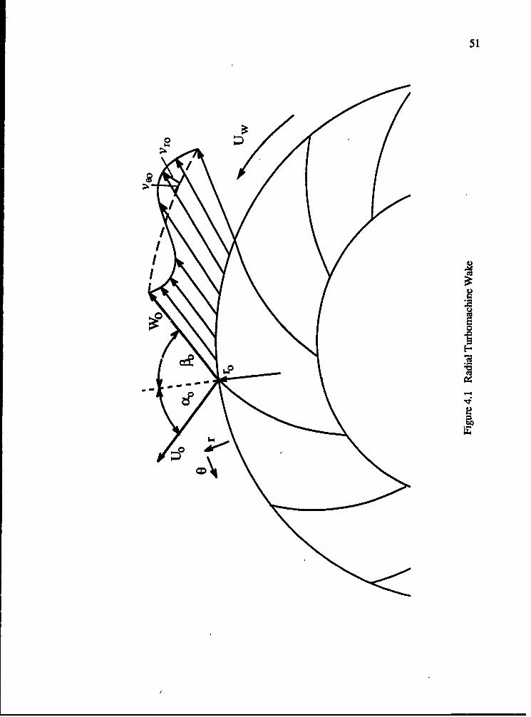
51

If/

I

I m ••mI •

C.)

(U

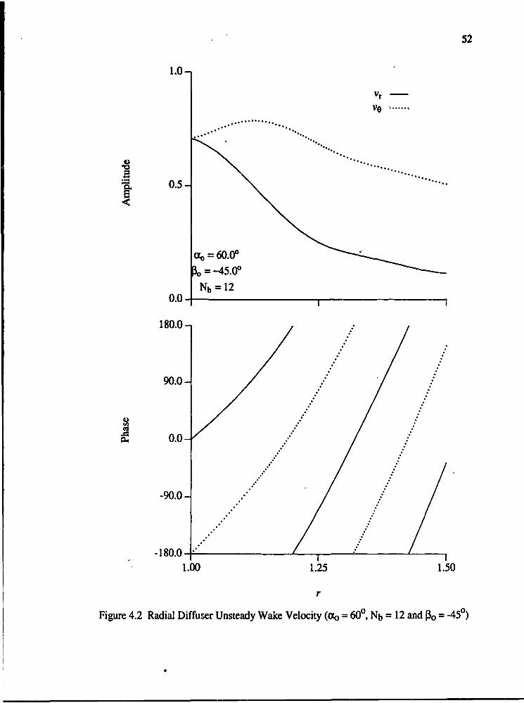
52

1.0-

Vr

SO O

0.5-

0 = 60.00

o =-45.0°Nb = 12

0.0-

180.0-

90.0-

0.0-

-90.0-

-180.0 -.

1.00 1.25 1.50

r

Figure 4.2 Radial Diffuser Unsteady Wake Velocity (xo = 600, Nb = 12 and 0o = -450)

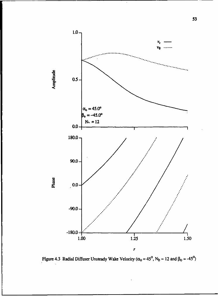
53

1.0-

Vr

0.5-

0 = 45.00

ro =-45.00N. -12

0.0

180.0-

90.0-

0.0-

-90.0-

-180.0-•1.00 1.25 1.50

r

Figure 4.3 Radial Diffuser Unsteady Wake Velocity (o0 = 450, Nb = 12 and 13o = -450)

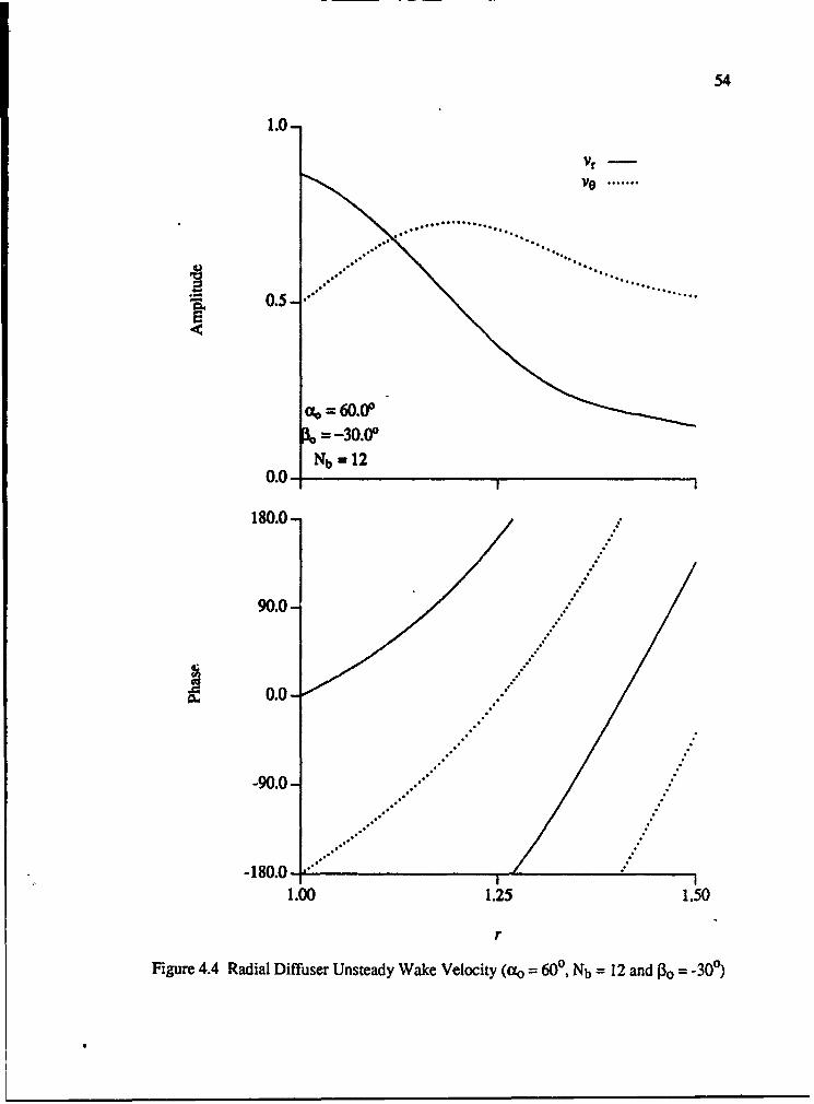
54

1.0-

vrSV o .. .....

0.5-

~x60.00

=-30.0oNb =12

0.0-

180.0-

90.0

"0.0

-90.0

-180.0-1.00 1.25 1.50

r

Figure 4.4 Radial Diffuser Unsteady Wake Velocity (Oxo = 60P, Nb = 12 and P3o = -300)

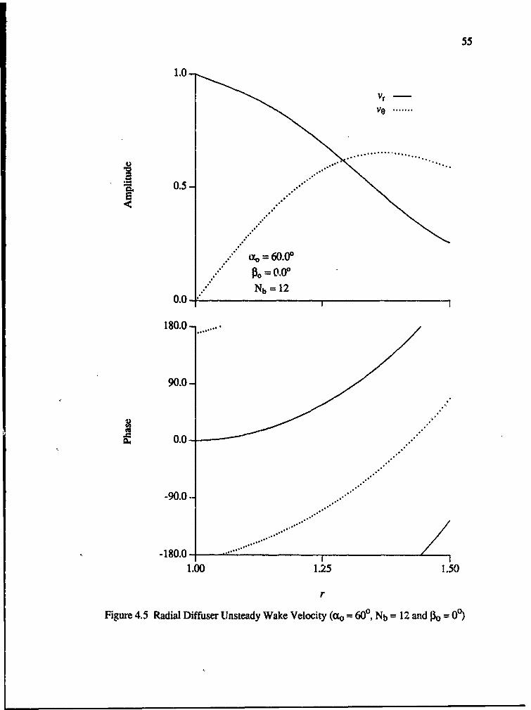
55

Vr

ve .......

0.5-

.... ao-60.0o... "" 13o =0.0,

Nb = 12

180.0

90.0

0.0-

-90.01- ..

1.00 1.25 1.50

r

Figure, 4.5 Radial Diffuser Unsteady Wake Velocity (aO 600, Nb =12 and 00 = 00)

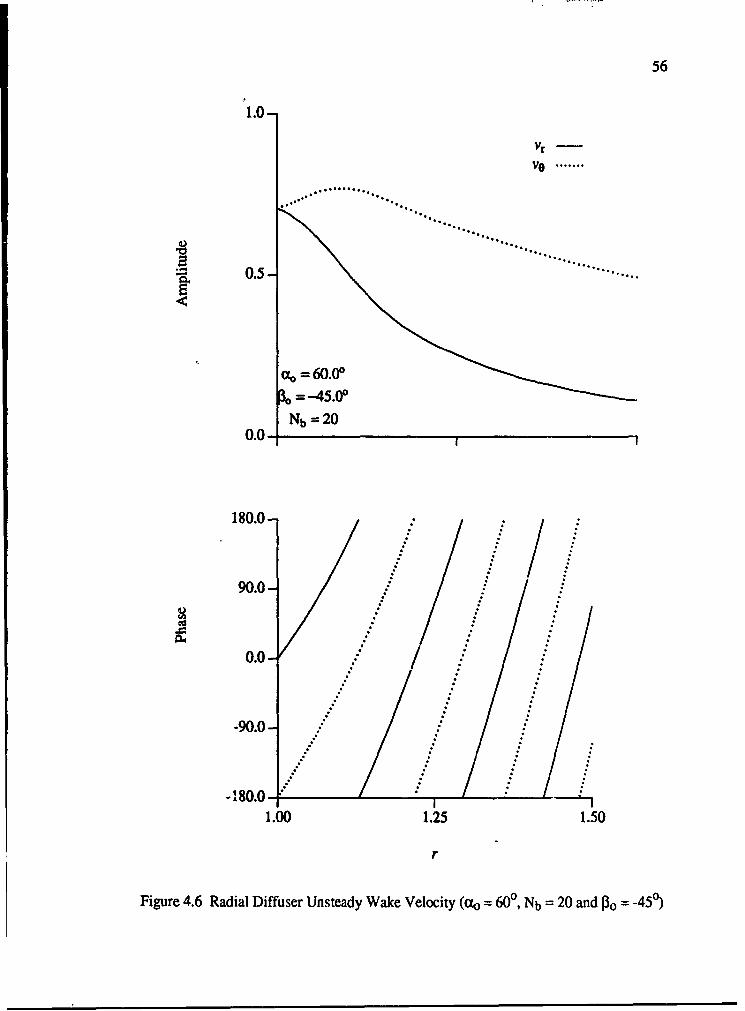
56

1.0-

VrVe ......

• ~0.5-".....

ao =60.00

o. = 45.0o

Nb =20

180.0

90.0-

0.0-

-90.0-

-'80.0 i -1.00 1.25 1.50

r

Figure 4.6 Radial Diffuser Unsteady Wake Velocity (czxo 600, Nb =20 and P~O = 450)

57

CHAPTER 5

RADIAL CASCADE UNSTEADY AIRFOIL THEORY

Much attention has been devoted in the literature to the unsteady aerodynamics ofisolated airfoils and axial flow cascades. In contrast, relatively little attention has beendirected at unsteady flow in radial cascades, with the experimental investigations of Inoueand Cumpsty (1984) and Arndt et al. (1988) two of the few examples. Radialturbomachine cascade flow fields and geometries are different than those for axial flowmachines. Due to these differences, axial flow cascade unsteady aerodynamic models arenot directly applicable to radial flow cascades. Thus, unsteady aerodynamic modelsapplicable to radial flow airfoil cascades are needed.

An analysis is developed to predict the unsteady fluid dynamics of radial flow cascadeswhile taking advantage of the existing research for axial flow turbomachines. This isaccomplished by developing a conformal transformation which allows a potential flowsolution for a given axial flow cascade to be applied to a radial cascade (Smith, 1970;Faulders, 1956). Thus, this transformation mathematically unwraps the steady andunsteady flowfields in a radial cascade into a corresponding axial cascade flow. Thistransformation is then coupled to an incompressible flat plate cascade analysis (Whitehead,1960; 1978). The effects of the cascade geometry on the unsteady fluid dynamics of radialcascades are then demonstrated by applying this rmodel to a series of radial flow cascadegeometries.

5.1 Transformation AnalysisFor a two-dimensional, incompressible and irrotational flow, the velocity potential 0 is

described by the Laplace equation.

ax2 y2 5.1

58

From the theory of complex variables, any function 0 of the cartesian variables x and y

which satisfies the Laplace equation can be expressed solely in terms of the complexvariable z = x + iy. Also, a conjugate function V exists such that the complex potential,w = 4) + iV is a function only of the complex variable z, with 0) and V individually

satisfying the Laplace equation (Churchill, 1984).The converse is also true. Given any function of a complex variable 71 + i4 = f(z),

the real and imaginary components of ý individually satisfy the Laplace equation providedC is an analytic function of z. Any complex function of a complex variable,S= fl(x,y) + i4(x,y) = f(x+iy) can also be considered a transformation from the variables xand y to the variables Tl and 4. In this case, the transformation is termed a conformal

transformation.If a solution to the Laplace equation can be found for a given geometry, the solution in

any other geometry can be found by applying an appropriate conformal transformation.For a radial cascade, the simple transformation given in Equation 5.2 transforms thesolution to a two-dimensional, infinite, axial flow cascade, as depicted in Figure 5.1.

S= ln z 5.2

where z is the coordinate in the radial diffuser and C is the coordinate in the transformed

plane. Thus, this transformation unwraps the steady and unsteady radial cascade flow

fields into those of a corresponding axial cascade. This allows a potential flow solution fora given axial cascade to be applied to a corresponding radial cascade.

Steady potential flow streamlines in a parallel wall radial diffuser follow logarithmic

spirals as shown in Chapter 1 and given in Equation 5.3.

In (L) =_ _r2 tanl 0L 5.3

where aOL is the angle between the streamline and a radial line, i.e., aL is the logarithmicspiral angle, r denotes the radius, r2 is a reference radius and 0 is the angular coordinate.

These streamlines are transformed into parallel straight streamlines by Equation 5.2. Thus,the flat plate airfoils in axial flow unsteady aerodynamic models are transformed intologarithmic spiral airfoils in the radial cascade.

59

A modified form of the transformation specified by Equation 5.2 is used for the actualconformal transformation. Namely, the transformation given in Equation 5.4 is utilized tomaintain the Kutta condition through the transformation in the unsteady flow.

S= r2 (In z - In r2) 5.4

where z is the coordinate for the radial geometry and ý is the coordinate for the transformed

axial geometry. Equation 5.4 expressed in radial coordinates is,

'1 + it = r2Qn (-) + ie)

The velocities in the two coordinate systems are related by Equation 5.6.

U -iU =2 =* UriUe 5.6

where U- and U4 are the axial cascade velocity components in the axial and tangentialdirections respectively, with Ur and U0 denoting the radial cascade velocity components inthe radial and tangential directions.

The Kutta condition, applied to both the steady and unsteady flow fields, is maintainedthrough the transformation. In a steady incompressible, inviscid flow, the pressure at anypoint in the flowfield is given by the following Bernoulli equation.

2p., U.2p 2 p 2 5.7

Since the right hand side of Equation 5.7 is constant, the steady pressure isproportional to the square of the steady velocity. Kutta's hypothesis requires that the

pressure be continuous at the airfoil trailing edge and that the trailing edge velocity is finite.Therefore the velocities on the upper and lower airfoil surfaces must approach a commonvalue at the trailing edge. Since the upper and lower velocities are scaled by the same r/r2as appears in the radial coordinate form of the transformation, Equation 5.5, the Kuttacondition requirement of no steady pressure discontinuity at the airfoil trailing edge issatisfied automatically independent of the value of r2.

60

The unsteady pressure is described by the following incompressible unsteady Bernoulli

equation.

P + 2 + P-. U.,2

p 2 p 2 5.8

In axial flow cascade linearized aerodynamic mode!s, the unsteady flow is considered

to be an harmonic small perturbation to a steady uniform mean flow in the chordwise

direction. In the chordwise direction, the pressure, velo:ity components, and velocity

potential are thus given by Equation 5.9.

p = P + jiexp (-i (0 t) 5.9a

u = U + fexp (-i o t) 5.9bv = v exp (-i o t) 5.9c

= 0 + exp (-i (a t) 5.9d

where P, 0, and U are the steady values of the pressure, velocity potential and freestream

chordwise velocity, with F, j, U and V the complex amplitudes of the unsteady pressure,

velocity potential, and choniwise and normal velocity components which are functions only

of the spatial coordinates. Note that in the axial flow cascade, U and P are constant. In the

radial cascade, U is proportional to 1/r and P is proportional to 1r 2.The linearized unsteady Bernoulli equation, Equation 5.10, is determined by

substituting Equation 5.9 into Equation 5.8 and retaining only first order terms in the

perturbation quantities.

p+ -U - i" = F(t)P 5.10

Applying the iinearized unsteady Bernoulli equation to the upper and lower surfaces of

a reference airfoil in either the axial or radial cascade results in the following equation for

the complex unsteady pressure difference across the reference airfoil chordline.

p = -U (5u.- 1 + i -P 5.141

61

The value of the velocity potential ý at each point in the axial cascade is the same as at

its image point in the corresponding radial cascade. However, the axial cascade velocity

and velocity components must be multiplied by the metric of the transformation, I/(r/r2).

Thus, the first term on the right hand side of Equation 5.11 must be multiplied by 1/(r/r2) 2.

For the pressure to be continuous and therefore the pressure difference across the airfoil tovanish at the trailing edge, r/r2 must be equal to unity at the trailing edge, i.e., the radialcascade airfoil trailing edge is defined by r = r2.

5.2 Cascade ModelFor a flat plate axial flow cascade at zero incidence in an incompressible flow, the

parameters necessary to specify the problem are the solidity, c/s, the reduced frequency,k = oc/U, the stagger angle, o, and the interblade phase angle, Ob. For the radial cascade,

the important parameters are the number of radial airfoils, Nv, the airfoil radial extentdivided by the trailing edge radius, Ar/r2, the reduced frequency based on the airfoil leadingedge velocity, k = wc/Ui, the stagger angle, ;, which is equal to the logarithmic spiralangle, aL, and the interblade phase angle, Ob.

Figure 5.2 shows the flat plate axial flow cascade transformation of a radial cascade.To apply existing axial flow cascade unsteady aerodynamic analyses to radial cascades, it isnecessary to determine the axial cascade parameters which correspond to a specified radial

cascade geometry. Given the parameters defining the radial cascade, the appropriatecorresponding parameters for the axial cascade unsteady aerodynamic models are calculatedthrough the transformation specified in Equation 5.5. In the following equations,unsubscripted values refer to the radial cascade and values with the A subscript refer to theaxial cascade transformation of the radial cascade.

The chord in the transformed axial cascade is given by Equation 5.12

CA = -r2 In (I - Ar/r2)cos a 5.12

The transformed axial cascade solidity, cA/sA is

A= -Nv In(I - Ar/r2)sA 2n csc 5.13

62

The relationship between the reduced frequencies for the axial and radial cascades is given

by

kA=A In (I - Atrk)kA=-k(Ar/r2)(1 - Ar/r2 ) 5.14

where k is the radial cascade reduced frequency.

The state-of-the-art axial flow cascade unsteady aerodynamic models predict the

unsteady aerodynamic lift and moment as well as the pressure distribution for airfoils

executing translational and torsional motions and subjected to convected harmonic vortical

gusts. The unsteady pressure difference, and unsteady lift and moment coefficients for

translation, torsion and gust are defined as

C AP _ Ap A p AppUA' pU2a 'pUv 5.15a

cL = _LWLq Lift .. AifpUh c pU2ac 'pUv c 5.15b

CM = Moment Moment Moment

pU/ic 2 pU2a c2 pUV c2 5.15c

where h and a are the translation and torsion airfoil motions h = ho exp (-i k t),

a= ao exp (-i k 0 and v is the wake or gust velocity at the airfoil leading edge,

v = vo exp (-i k t). In the previous expressions, ho, a0 and vo are the motion and velocity

amplitudes. In the radial cascade, U and v are the values at the airfoil leading edge.

The unsteady pressure distribution for the radial cascade is calculated from the unsteadyvelocities in the axial cascade through the transformation defined by Equations 5.5 and 5.6,

with the unsteady aerodynamic lift and moment coefficients calculated from this by

integration.

5-3 Bounda Condition TransformaonThe radial cascade logarithmic spiral airfoils undergoing translation and torsion motions

do not transform exactly to flat plates in the axial cascade undergoing the same motions.

63

To correct for this, the airfoils in the radial cascade are assumed to undergo small amplitude

torsional and translation motions, Figure 5.3, with the corresponding motions in the axial

cascade calculated through the transformation, Equation 5.5. The translation and torsion

boundary conditions in the form of upwash velocities for the radial cascade are given in

Equations 5.16 and 5.17.

dt 5.16

v = Ua + 'd(x - x5.1dt 5.17

where x is the distance along the vane nondimensionalized by the chord and Xea is the

nondimensional elastic axis location defined in Figure 5.2.In classical isolated airfoil and axial flow cascade unsteady aerodynamic models,

upstream airfoil wakes are modeled by convected harmonic gusts, Figure 5.4. The

behavior of these convected gusts was discussed in Chapter 4, with the radial and

tangential unsteady velocity components shown again in Equations 5.18 and 5.19.

Vr= r(nO rk2-1 exp(AInr+Br2)rl -k2dr -

r-k2- If exp(A In r+ B r 2) rl + k2 drexp(ik(O.- t )) +

( A2i rk2 1+ k2a2 rk2 .1) exp(ik(O - t)) 5.18ro ro

and

aip ý= 4E .( rk2-1 exp(A In r + Br2) rI - k2 dr +

r-k2 1 f exp(AIn r+B r 2) rl + k2 drexp(ik(O- t)) +

(k2a Ark2"ro I+k2r-o k2 "1) exp(ik(O") 5.19

64

From these velocity components, the normal velocity induced by the wakes on the airfoilsurfaces is computed, Equation 5.20.

Vn = VrSin oto - voos (ore 5.20

The translation, torsion and wake boundary conditions in the radial cascade, Equations5.16, 5.17 and 5.20, are transformed to the axial flow cascade using the velocitytransformation, Equation 5.6. The results are presented in Equations 5.21 throuth 5.23.

VhA = dt/(r/r2) 5.21dt 52

Ua + "a x - X'.VatA -- i .... (l

r/r2 5.22

vnA rSin o - v!cos acor/r2 5.23

The expressions for the radial cascade wake behavior, Equations 5.18 and 5.19, cannotbe evaluated for k2 < 2, due to the fact that CIO cannot be chosen so that the wake velocities

will remain bounded as r -*m. Because of this, the standard axial cascade upwash,

Equation 5.24, is used in the transformed axial cascade at low reduced frequency.

v = vo exp(ik'AX - ikAt) 5.24

where the reduced frequency, kA, is equal to the transformed reduced frequency in

Equation 5.14, and kJA is a transformed boundary condition reduced frequency. This

separate reduced frequency occurs due to the deceleration of the steady flow with radius,thus decreasing the wavelength of the wake.

The transformation reduced frequency, Equation 5.14, is necessary due to the chordlength change through the transformation and also the change in velocity at the leadingedge. The reduced frequency in the boundary condition, Equation 5.24, is the ratio of thechord, c, to the gust wavelength, U/m, thus determining the number of wake wavelengthson the vane. Due to the velocity decrease with radius in the radial cascade, the gust

65

wavelength becomes smaller toward the wailing edge. The transformed boundary condition

reduced frequency is then

k'A=k (2 - Ar/r 2)2(l - Ar/r 2) 5.25

The boundary condition, Equation 5.20, is only necessary at low k, with the more

physically realistic wake velocities in Equations 5.18 and 5.19 used at higher values of k

which would be encountered in real machines.

5.4 Model VerificaionTo validate the transformation technique and radial cascade modeling, the radial cascade

unsteady aerodynamic lift and moment are predicted for the special case of Ar/r2 --)0. In

this case, the radial cascade flowfield approaches that of an axial flow cascade. The radialcascade parameters are Nv = 300, a = 600, Ar/r2 = 0.01 and rea = 0, as defined in Figure

5.2. For the axial cascade, s/c = 1.0, a = 600, and Xea = 0. The number of airfoils in the

radial cascade was chosen to give a transformed axial cascade solidity of 1.0.

Figures 5.5 through 5.10 show the unsteady lift due to translation, the unsteady

moment due to torsion and the unsteady lift due to a transverse gust for both the baseline

axial and radial flow cascades over a range of reduced frequencies and interblade phase

angles. The predicted unsteady aerodynamics of the baseline radial cascade approach thatof the axial cascade, thereby verifying the transformation and the radial cascade unsteady

aerodynamic modeling.

5.5 Results

The fundamental differences between radial and axial cascade unsteady aerodynamics

are considered by utilizing this model to predict radial and correspording axial cascade

unsteady aerodynamics. In particular, the unsteady aerodynamic translational lift, torsionalmoment, and convected gust lift as well as the corresponding unsteady pressuredistributions are analyzed. The baseline radial cascade parameters are Nv = 12, ; = 600,

Ar/r2 = 0.25 and rea = 0. The baseline geometry differs from the previous cases only in

66

that the vane radial extent, Ar/r2, is greater, thereby demonstrating the effects of the radial

geometry.Figure 5.11 shows the unsteady aerodynamic translational lift, CL, for the baseline

radial cascade as a function of the reduced frequency and interblade phase angle. For this

translational response, the unsteady lift will amplify the motion when the real part of CL is

positive, indicating a possible flutter condition. For both the axial and radial cascades, allpoints shown have negative real values and thus are stable. Also, the stability margins for

both cascades are similar. The unsteady lift amplitude for the radial cascade is slightlyhigher in general than the axial flow cascade.

Figure 5.12 presents the unsteady aerodynamic torsional moment, CM, for the baselineradial cascade as a function of the reduced frequency and interblade phase angle. In this

case, the imaginary part of CM determines stability, with a stable cascade for CM < 0. Thestability is similar for both the axial and radial cascades, with the zero reduced frequencyresults unstable for both cascades, but all other reduced frequency configurations stable.As for the translational response, the interblade phase angle has a lesser effect on theunsteady moment for the radial cascade than for the axial. The unsteady momentamplitudes are greater for the axial cascade at low reduced frequency and become roughlyequal at higher reduced frequcncy.

The unsteady aerodynamic response of the baseline cascade to a convected transversegust as a function L. ' .h'e reduced frequency and interblade phase angle is shown in Figure5.13. Since the reduced frequency is low (k < 2), the standard axial cascade upwash,Equation 4.2, is usd! in the transformed axial cascade. As with the translational andtorsional responses, Figure 5.10 shows that the interblade phase angle has a lesser effect inthe radial cascade than the axial cascade. The unsteady lift amplitude is smaller for theradial casc,-4e than the axial.

Figures 5.14 and 5.15 show the unsteady airfoil pressure difference CAp due totranslation and torsion for a single reduced frequency/interblade phase angle combinationfrom each of Figures 5.11 through 5.13. Theunsteady pressure difference is presented forthe radial cascade and for the axial cascade conditions of Figures 5.5, 5.7 and 5.9. Theunsteady pressure is greater for the radial cascade undergoing plunging motions which isconsistent with Figure 5.11. The unsteady pressure due to pitching is greater at the airfoilleading edge for the radial cascade and greater at the trailing edge for the axial cascade.

Figure 5.16 shows the unsteady airfoil pressure difference due to a convected gustupwash for radial and axial flow cascades. In this figure, k = 2 and Ob = 00, with the

transformed cascade upwash given by Equation 5.20. In Figure 5.17, k = 4 and the radial

67

cascade airfoil pressure difference with the wake model upwash, Equations 5.18 and 5.19,

is shown. The axial cascade unsteady pressure is greater than the radial cascade, consistent

with Figure 5.13. In Figure 5.17, the axial cascade unsteady pressure is greater than the

radial cascade with the standard upwash, Equation 5.20, but is less than the radial cascade

with the wake model upwash, Equations 5.18 and 5.19. Using these more physically

realistic wake expressions increases the predicted radial cascade lift

In Chapter 6, the unsteady diffuser vane pressure distribution measured in the Purdue

Centrifugal Cownpressor Facility will be presented. The preceding analysis will be

compared with the measured data.

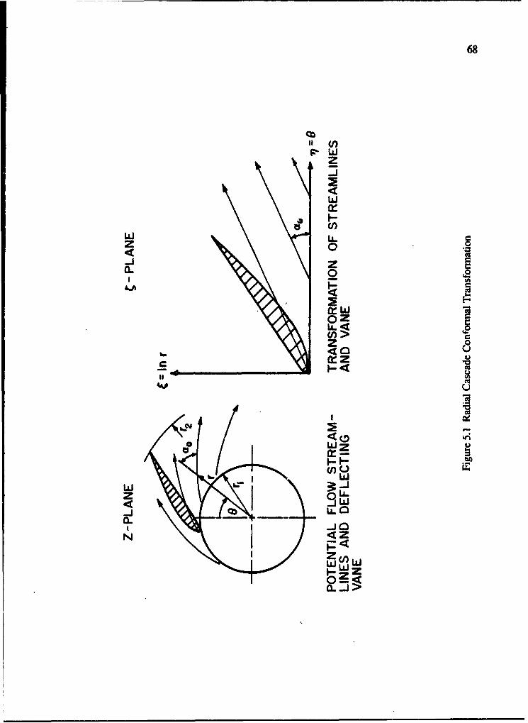
68

zz

CL 0)

z 0

mz2u

WCA

tw Iz 0 Utrz

CL

44z C/U

wwI--

R-i

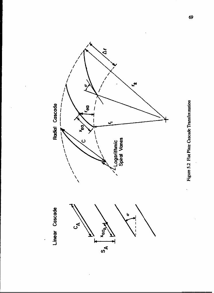
69

CP.Lin0

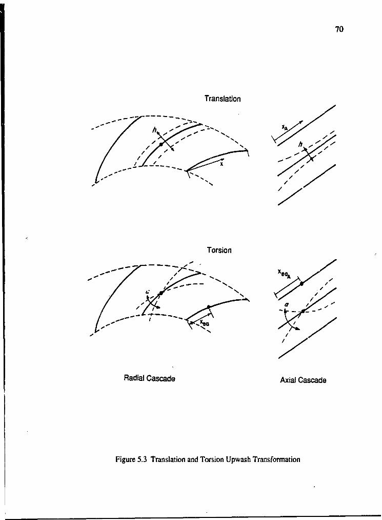
70

Translation

- -h - - -- XA lo,

// /

Torsion

-XOA

Radial Cascade Axial Cascade

Figure 5.3 Translation and Torsion Upwash Transformation

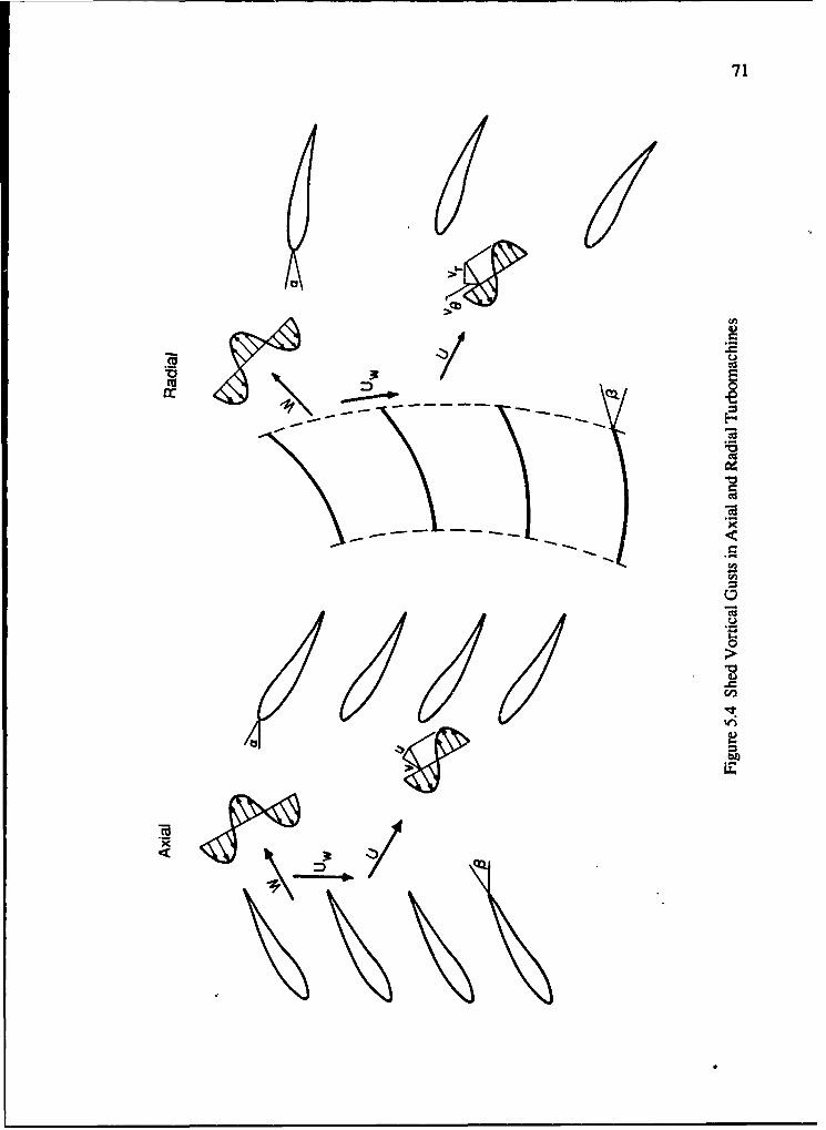
71

9cca DCOEiU)

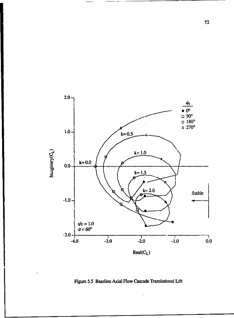
72

2.0-

0900

o 18o?2700

1.0- k=0.5

k= 0.0*Go 0.0-

Sk= 1.5

k= 2.0 Stable

-1.0

s/c = 1.0a•=600

-2.0 - 1- I 1 1-4.0 -3.0 -2.0 -1.0 0.0

Real(CL)

Figure 5.5 Baseline Axial Flow Cascade Translational Lift

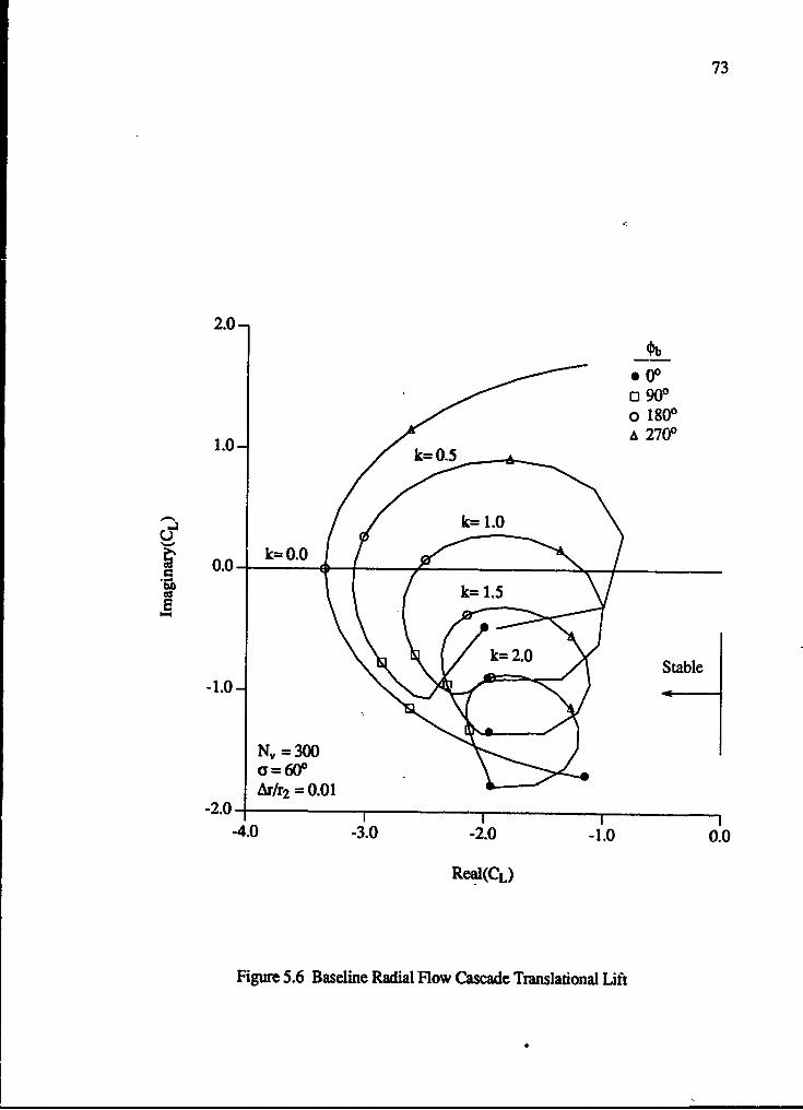
73

2.0-

.000o 900o 1800

1.0-k0. A 2700

U

0.0- k .

'U k= 1.5

-1.0k= 2.0 Stable

N,, = 300(y=600Ak= 0.01

-2.0-i I I-4.0 -3.0 -2.0 -1.0 0.0

Real(CL)

Figure 5.6 Baseline Radial Flow Cascade Translational Lift

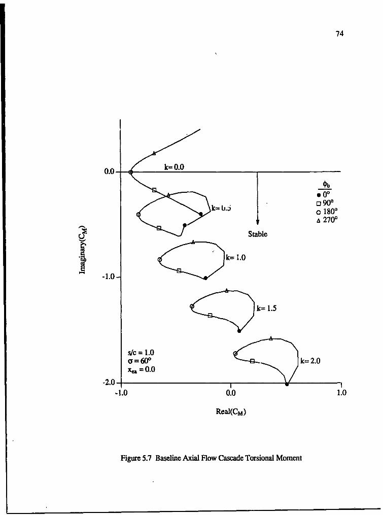
74

0.0-

.00S0900

o 180'& 270"

SStable

k= 1.0

LC" -1.0-

k= 1.5

s/c = 1.0(T = 60°/ k= 2.0X..= 0.0

-2.0 - -- 1-1.0 0.0 1.0

Real(CM)

Figure 5.7 Baseline Axial Flow Cascade Torsional Moment

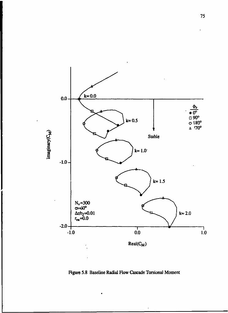
75

0.0- k=O0.0_____ ____

O~b

_00oa900k= 0.5 o 980

A 1700

Stable

k= 1.0"

-1.0-

k= 1.5

N,=300

Ar/r2=0.01 k= 2.0r,.=0.0

-2.0 -

-1.0 0.0 1.0

Real(CM)

Figure 5.8 Baseline Radial Flow Cascade Torsional Moment

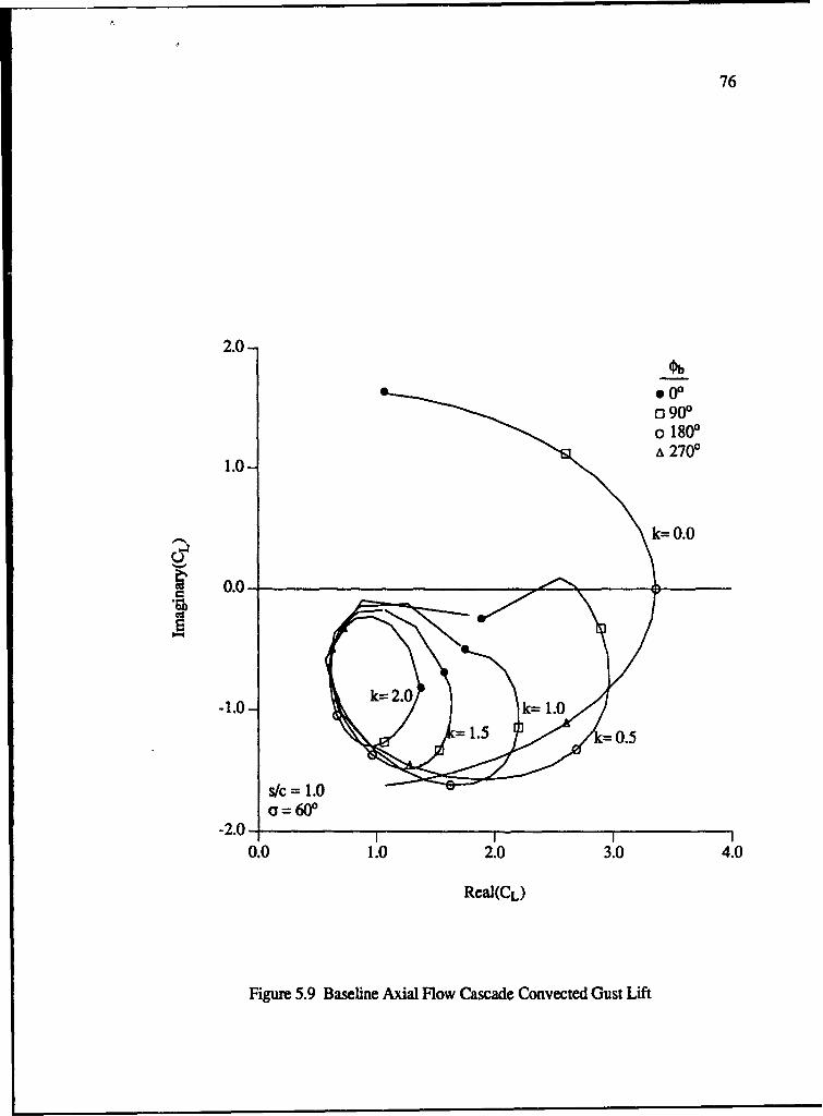
76

2.0-

.00o 90°o 1800A 2700

1.0-

•k 0.0

0.0-

-1.0-1.5 0.5

s/c= 1.0; = 600

-2.0 1111 SI II

0.0 1.0 2.0 3.0 4.0

Real(CL)

Figure 5.9 Baseline Axial Flow Cascade Convected Gust Lift

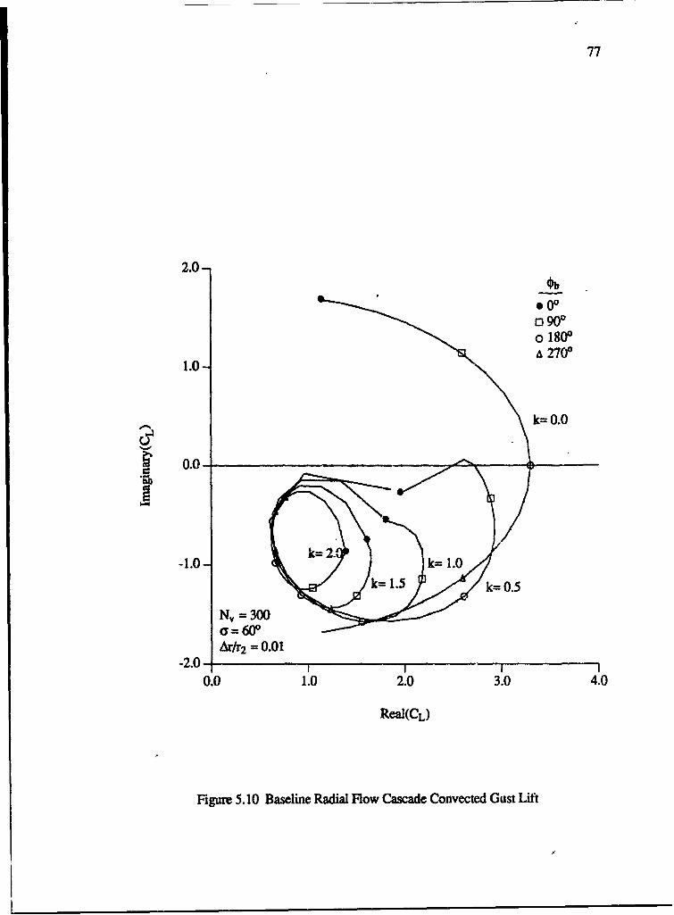
77

2.0-Ob

0000]90,

o 1800A 2700

1.0-

k= 0.0

0.0-

-1.0- k= 2. k= 1.0

k= 1.5 k= 0.5

N, =300a= 60° 1

Ark = 0.01-2.0 1 1 1 10.0 1.0 2.0 3.0 4.0

Re~a(CL)

Figure 5.10 Baseline Radial Flow Cascade Convected Just Lift

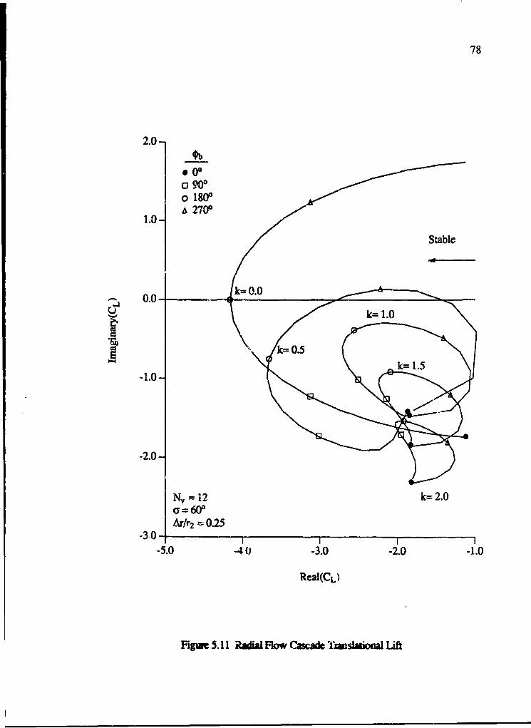
78

2.0- I b.0oo 900o 1800A 27001.0-

Stable

0.0--k0.0k= 1.0

-2,0-

N,,= 12 k= 2.0

Arlr2 - 0.25-3.0,

-5.0 -40 -3.0 -2.0 -1.0

ReWa(CL)

Figmu 5.11 Rial Flow C "scs'mnsliaonal Lift

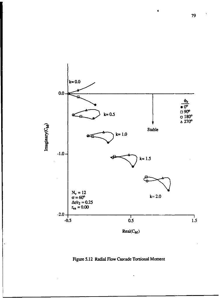
q

79

k= 0.0

0.0-

.01

k= 0.5 o 8900o 1800A 2700

Stablek= 1.0

-1.0-k= 1.5

N= 12a=60P k= 2.0At/r2 = 0.25r,ý =0.00

-2.0 - 1-0.5 0.5 1.5

Real(CM)

Figure 5.12 Radial Flow Cascade Torsional Moment

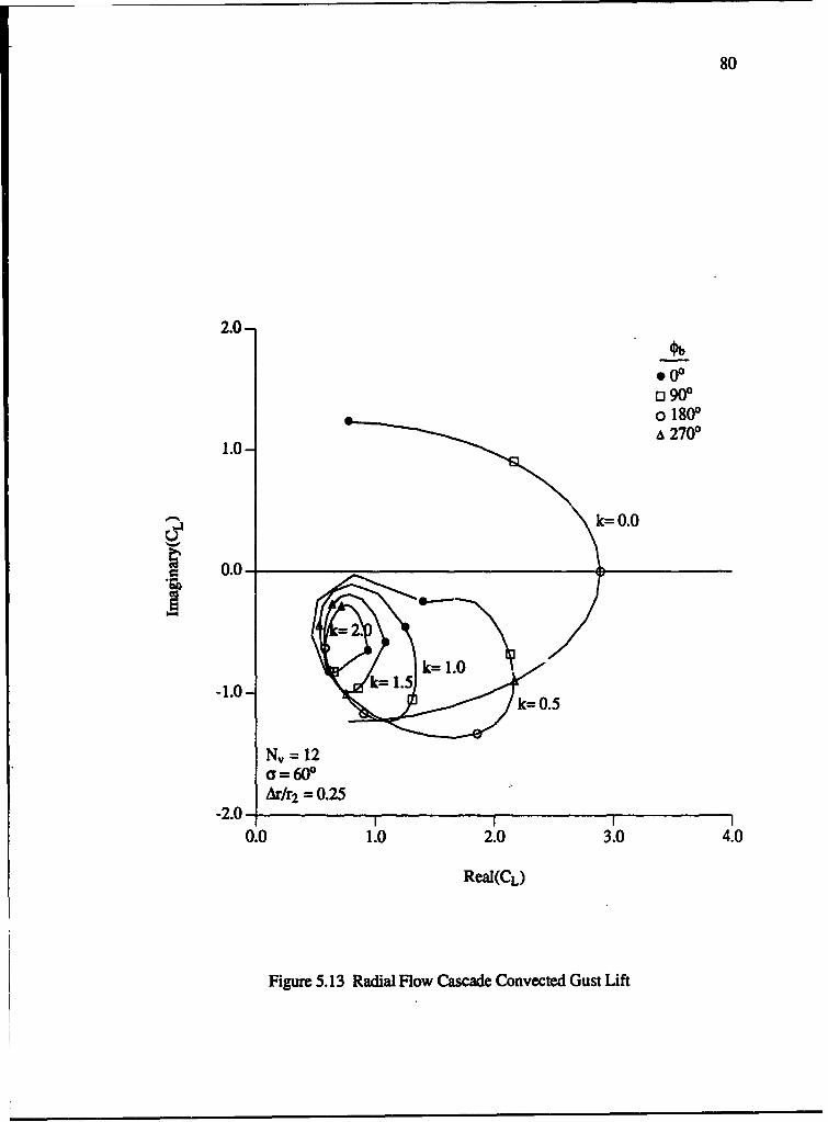
80

2.0-

9(oo1800

92700

1.0-

0.0-S0.0

-1.0 1.0k= 1.5

N,= 12a=600

Ar/r2 = 0.25I I II

0.0 1.0 2.0 3.0 4.0

Real(CL)

Figure 5.13 Radial Flow Cascade Convected Gust Lift

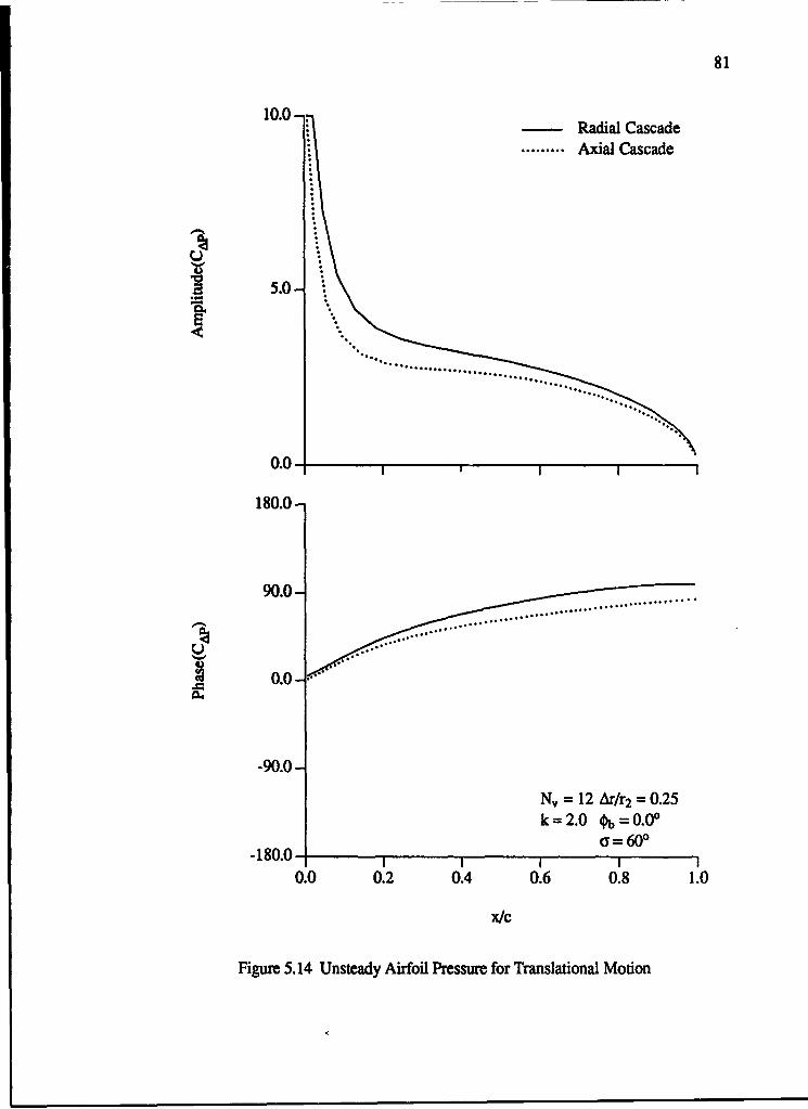
81

10.0 -Radial Cascade

......... Axial Cascade

0!

5.0-

0.0- I

180.0-

90.0-

M= 12 &r/r2 =0.25k=2.0 4 = 0.0o

a =600-180.0

c 0SIi I

0.0 0.2 0.4 0.6 0.8 1.0

x/c

Figure 5.14 Unsteady Airfoil Pressure for Translational Motion

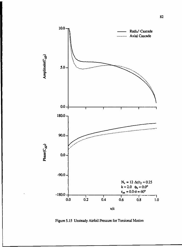
82

10.0-RadiO~ Cascade

..... Axial Cascade

0.0-

180.0-

90.0-

0.0-

-90.0-

N, 12 Ar/r2 0.25k =2.0 Ob= 0.00

-180.0r., = 0.Oa= 600

0.0 0.2 0.4 0.6 0.8 1.0

x/C

Figure 5.15 Unsteady Airfoil Pressure for Torsional Motion

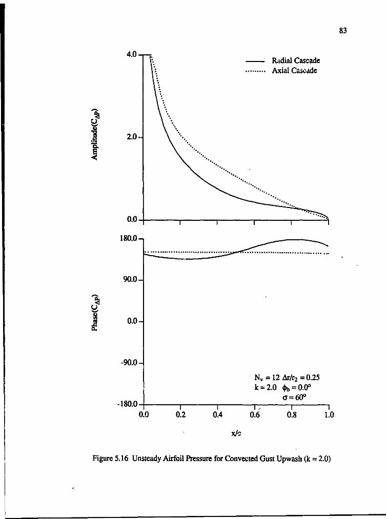
83

4.0- Radial Cascade

......... Axial Cascade

2.0-

0.0- I-....

180.0-

90.0-

0.0

-90.0-

N= 12 Ar/r2 = 0.25k=2.0 O=0.00

=60°-180.0 i I i ,,6

0.0 0.2 0.4 0.6 0.8 1.0

Figure 5.16 Unsteady Airfoil Pressure for Convected Gust Upwash (k = 2.0)

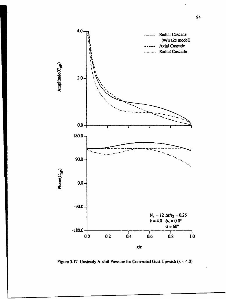
84

4.0- - Radial Cascade

(w/wake model)- Axial Cascade

......... Radial Cascade

r•2.0-

...................... . •. . €.. ...... ..

004

0.0-- I I I

180.0 -

..................

04.0

S~0.0-

-90.0 -

Nv= 12 Ar/r2 =0.25k=4.0 4o = 0.0'

a=60*-100II I

0.0 0.2 0.4 0.6 0.8 1.0

x/c

Figure 5.17 Unsteady Airfoil Pressure for Convected Gust Upwash (k = 4.0)

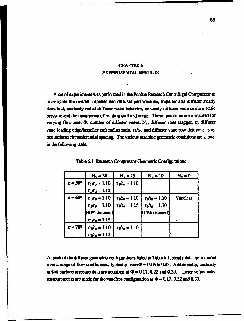
85

CHAPTER 6EXPERIMENTAL RESULTS

A set of experiments was performed in the Purdue Research Centrifugal Compressor to

investigate the overall impella and diffuser performance, impeller and diffuser steady

flowfield, unsteady radial diffuser wake behavior, unsteady diffuser vane surface static

pressure and the occurnce of rotating stall and surge. These quantities are measured forvarying flow ramte, 0, number of diffuser vanes, Nv, diffuser vane stagger, a, diffuser

vane leading edge/Impeller exit radius ratio, rifro, and diffuser vane row detuning using

nonuniform cir.cumferential spacing. The various machine geometric conditions are shown

in the following table.

Table 6.1 Research Conpressor Geometric Configuadons

NV = 30 M= 15 - N = 10 N, = 0a=50" ri/ro=1.10 r/ro= 1.1O

r_/ro = 1.15

S=60W ril/ro = 1.10 rlr0o=1.10 ril/ro=1.10 Vaneless

rl/ro = 1.10 rl/ro= 1.15 rl/ro= 1.10

(40o, deuned) 13% detuned)Ir__ ro = 1.15 ._

a=700 rl/ro= 1.10 rl/ro= 1.10

rl/rjr= 1.15

At each of the diffuser gooneuic configuration listed in Table 6.1, steady data are acquiredover a range of flow coefficients, typically from 0 = 0.16 to 0.33. Additionally, unsteady

airfoil surface pressure data arn acquired at 0.= 0.17,0.22 and 0.30. Laser velocimetermeasurements are made for the vaneless configuration atO = 0.17,0.22 and 0.30.

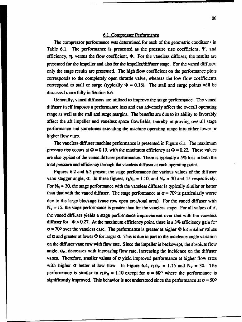
86

6.1 Compressor PerformanceThe compressor performance was determined for each of the geometric conditions in

Table 6.1. The performance is presented as the pressure rise coefficient, TP, andefficiency, il, versus the flow coefficient, 4. For the vaneless diffuser, the results arepresented for the impeller and also for the impeller/diffuser stage. For the vaned diffuser,only the stage results are presented. The high flow coefficient on the performance plotscorresponds to the completely open throttle valve, whereas the low flow coefficientscorrespond to stall or surge (typically 0 - 0.16). The stall and surge points will bediscussed more fully in Section 6.6.

Generally, vaned diffusers are utilized to improve the stage performance. The vaneddiffuser itself imposes a performance loss and can adversely affect the overall operatingrange as well as the stall and surge margins. The benefits are due to its ability to favorablyaffect the aft impeller and vaneless space flowfields, thereby improving overall stageperformance and sometimes extending the machine operating range into either lower orhigher flow rates.

The vaneless diffuser machine performance is presented in Figure 6.1. the maximumpressure rise occurs at 0 = 0.19, with the maximum efficiency at 0 = 0.22. These valuesare also typical of the vaned diffuser performance. There is typically a 5% loss in both thetotal pressure and efficiency through the vaneless diffuser at each operating point.

Figures 6.2 and 6.3 present the stage performance for various values of the diffuservane stagger angle, a. In these figures, rj/ro = 1.10, and Nv = 30 and 15 respectively.

For Nv = 30, the stage performance with the vaneless diffuser is typically similar or betterthan that with the vaned diffuser. The stage performance at a = 700 is particularly worsedue to the la-ge blockage (vane row open area/total area). For the vaned diffuser withNv = 15, the srage performance is greater than for the vaneless stage. For all values of a,the vaned diffuser yields a stage performance improvement over that with the vanelessdiffuser for 0 > 0.27. At the maximum efficiency point, there is a 3% efficiency gain fc:

-= 700 over the vaneless case. The performance is greater at higher 0 for smaller valuesof a and greater at lower 0 for larger Y. This is due in part to the incidence angle variation

on the diffuser vane row with flow rate. Since the impeller is backswept, the absolute flowangle, a•, decreases with increasing flow rate, increasing the incidence on the diffuservanes. Therefore, smaller values of Y yield improved performance at higher flow rateswith higher a better at low flow, In Figure 6.4, rj/ro = 1.15 and Nv = 30. Theperformance is similar to ri/ro = 1.10 except for a = 600 where the performance issignificantly improved. This behavior is not understood since the performance at a =500

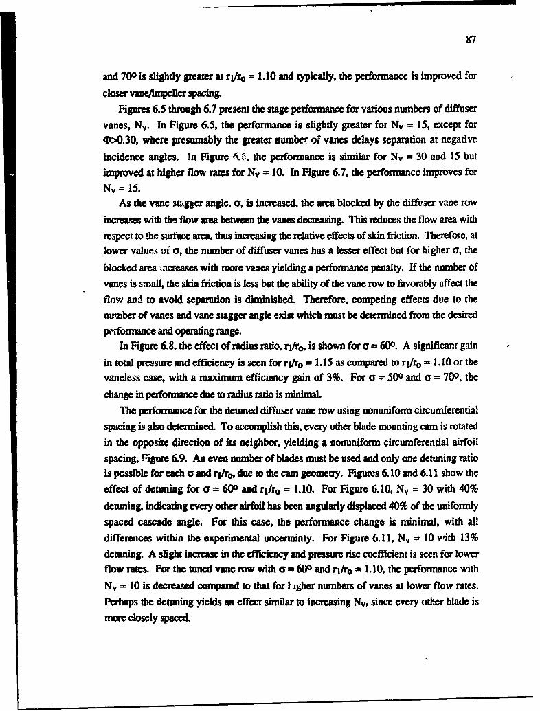
87

and 700 is slightly greater at ri/ro = 1.10 and typically, the performance is improved for

closer vanefimpeller spacing.

Figures 6.5 through 6.7 present the stage performance for various numbers of diffuser

vanes, Nv. In Figure 6.5, the performance is slightly greater for Nv = 15, except for0•0.30, where presumably the greater number of vanes delays separation at negative

incidence angles. )n Figure 6.C, the performance is similar for Nv = 30 and 15 but

improved at higher flow rates for Nv = 10. In Figure 6.7, the performance improves for

Nv = 15.As the vane stagger angle, a, is increased, the area blocked by the diffuser vane row

increases with thn flow area between the vanes decreasing. This reduces the flow area with

respect to the surface area, thus increasing the relative effects of skin friction. Therefore, atlower values of a, the number of diffuser vanes has a lesser effect but for higher a, the

blocked area increases with more vanes yielding a performance penalty. If the number of

vanes is small, the skin friction is less but the ability of the vane row to favorably affect the

flow and to avoid separation is diminished. Therefore, competing effects due to the

number of vanes and vane stagger angle exist which must be determined from the desired

prrformance and operating range.In Figure 6.8, the effect of radius ratio, rl/ro, is shown for a = 600. A significant gain

in total pressure and efficiency is seen for rl/ro = 1.15 as compared to rl/ro = 1.10 or thevaneless case, with a maximum efficiency gain of 3%. For Y = 500 and a = 700, the

change in performance due to radius ratio is minimal.

The performance for the detuned diffuser vane row using nonuniform circumferential

spacing is also determined. To accomplish this, every other blade mounting cam is rotatedin the opposite direction of its neighbor, yielding a nonuniform circumferential airfoil

spacing, Figure 6.9. An even number of blades must be used and only one detuning ratiois possible for each a and r/ro, due to the cam geometry. Figures 6.10 and 6.11 show the

effect of detuning for a = 600 and ri/ro = 1.10. For Figure 6.10, Nv = 30 with 40%

detuning, indicating every other airfoil has been angularly displaced 40% of the uniformly

spaced cascade angle. For this case, the performance change is minimal, with all

differences within the experimental uncertainty. For Figure 6.11, Nv = 10 with 13%

detuning. A slight increase in the efficiency and pressure rise coefficient is seen for lowerflow rates. For the tuned vane row with a = 600 and rl/ro - 1.10, the performance with

Nv = 10 is decreased compared to that for f i-her numbers of vanes at lower flow rates.

Perhaps the detuning yields an effect similar to increasing Nv, since every other blade ismore closely spaced.

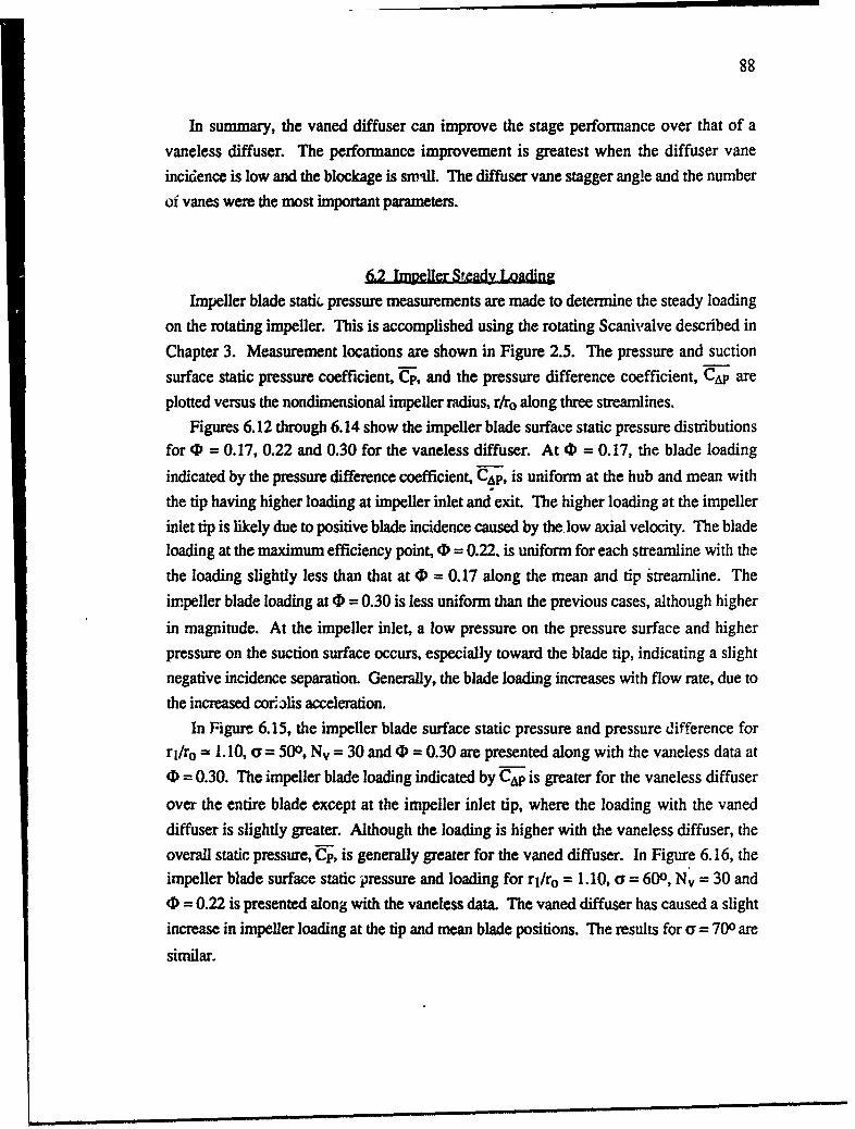
88

In summary, the vaned diffuser can improve the stage performance over that of avaneless diffuser. The performance improvement is greatest when the diffuser vane

incicdence is low and the blockage is smill. The diffuser vane stagger angle and the number

of vanes were the most important parameters.

6.2 Impeller Steady Loading

Impeller blade stati. pressure measurements are made to determine the steady loading

on the rotating impeller. This is accomplished using the rotating Scanivalve described in

Chapter 3. Measurement locations are shown in Figure 2.5. The pressure and suction

surface static pressure coefficient, CUp, and the pressure difference coefficient, CAp areplotted versus the nondimensional impeller radius, r/re along three streamlines.

Figures 6.12 through 6.14 show the impeller blade surface static pressure distributionsfor 4) = 0.17, 0.22 and 0.30 for the vaneless diffuser. At 0 = 0.17, the blade loading

indicated by the pressure difference coefficient, CAp, is uniform at the hub and mean with

the tip having higher loading at impeller inlet and exit. The higher loading at the impeller

inlet tip is likely due to positive blade incidence caused by the low axial velocity. The bladeloading at the maximum efficiency point, (D = 0.22, is uniform for each streamline with the

the loading slightly less than that at 4D = 0.17 along the mean and tip streamline. The

impeller blade loading at 4D = 0.30 is less uniform than the previous cases, although higher

in magnitude. At the impeller inlet, a low pressure on the pressure surface and higher

pressure on the suction surface occurs, especially toward the blade tip, indicating a slightnegative incidence separation. Generally, the blade loading increases with flow rate, due to

the increased coriolis acceleration.

In Figure 6.15, the impeller blade surface static pressure and pressure difference forrl/ro = 1.10, o-= 500, Nv = 30 and 4 = 0.30 are presented along with the vaneless data at

4D = 0.30. The impeller blade loading indicated by C•p is greater for the vaneless diffuser

over the entire blade except at the impeller inlet tip, where the loading with the vaneddiffuser is slightly greater. Although the loading is higher with the vaneless diffuser, the

overall static pressure, Cp, is generally greater for the vaned diffuser. In Figure 6.16, theimpeller blade surface static pressure and loading for rj/ro = 1.10, a = 600, Nv = 30 and0 = 0.22 is presented along with the vaneless data. The vaned diffuser has caused a slight

increase in impeller loading at the tip and mean blade positions. The results for a = 700 are

similar.

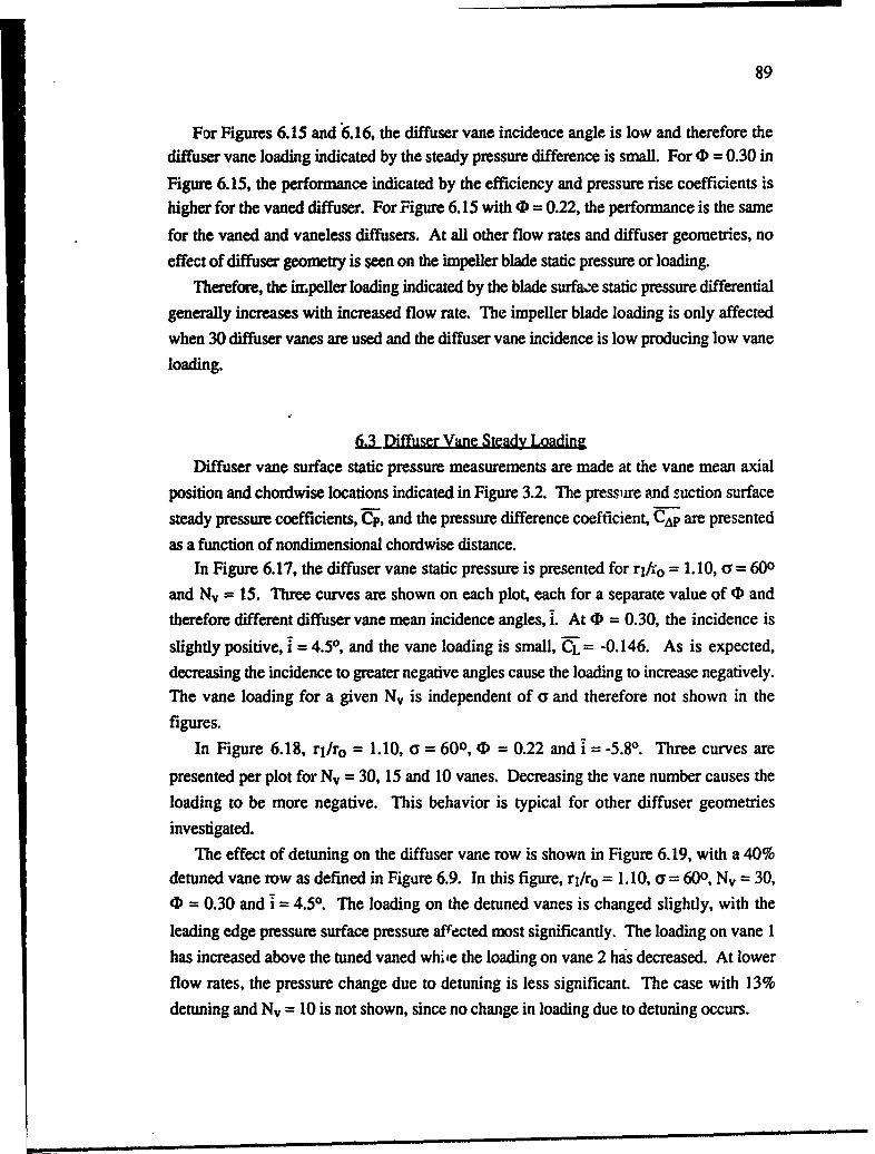
89

For Figures 6.15 and 6.16, the diffuser vane incidence angle is low and therefore thediffuser vane loading indicated by the steady pressure difference is small. For 0 = 0.30 inFigure 6.15, the performance indicated by the efficiency and pressure rise coefficients ishigher for the vaned diffuser. For Figure 6.15 with 0 = 0.22, the performance is the same

for the vaned and vaneless diffusers. At all other flow rates and diffuser geometries, noeffect of diffuser geometry is seen on the impeller blade static pressure or loading.

Therefore, the impeller loading indicated by the blade surfae static pressure differentialgenerally increases with increased flow rate. The impeller blade loading is only affectedwhen 30 diffuser vanes are used and the diffuser vane incidence is low producing low vaneloading.

6. Diffuser Vane Steady LoadingDiffuser vane surface static pressure measurements are made at the vane mean axial

position and chordwise locations indicated in Figure 3.2. The pressire and suction surfacesteady pressure coefficients, Cp, and the pressure difference coefficient, C•p are presentedas a function of nondimensional chordwise distance.

In Figure 6.17, the diffuser vane static pressure is presented for rl/;o = 1.10, a = 600and Nv = 15. Three curves are shown on each plot, each for a separate value of (D andtherefore different diffuser vane mean incidence angles, i. At 4D = 0.30, the incidence is

slightly positive, 1 = 4.50, and the vane loading is small, CL = -0.146. As is expected,

decreasing the incidence to greater negative angles cause the loading to increase negatively.The vane loading for a given Nv is independent of a and therefore not shown in the

figures.In Figure 6.18, rj/ro = 1.10, a = 600, 4) = 0.22 and i = -5.80. Three curves are

presented per plot for Nv = 30, 15 and 10 vanes. Decreasing the vane number causes theloading to be more negative. This behavior is typical for other diffuser geometriesinvestigated.

The effect of detuning on the diffuser vane row is shown in Figure 6.19, with a 40%detuned vane row as defined in Figure 6.9. In this figure, rl/ro = 1.10, a= 600, Nv = 30,

4D = 0.30 and 1 = 4.50. The loading on the detuned vanes is changed slightly, with theleading edge pressure surface pressure affected most significantly. The loading on vane 1has increased above the tuned vaned whi4e the loading on vane 2 has decreased. At lowerflow rates, the pressure change due to detuning is less significant. The case with 13%detuning and Nv = 10 is not shown, since no change in loading due to detuning occurs.

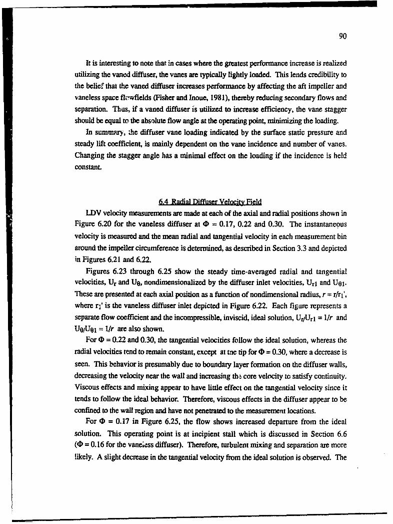
90

It is interesting to note that in cases where the greatest performance increase is realizedutilizing the vaned diffuser, the vanes are typically lightly loaded. This lends credibility tothe belieff that the vaned diffuser increases performance by affecting the aft impeller andvaneless space flewfields (Fisher and Inoue, 1981), thereby reducing secondary flows andseparation. Thus, if a vaned diffuser is utilized to increase efficiency, the vane staggershould be equal to the absolute flow angle at the operating point, minimizing the loading.

In summary, .he diffuser vane loading indicated by the surface static pressure andsteady lift coefficient, is mainly dependent on the vane incidence and number of vanes.Changing the stagger angle has a minimal effect on the loading if the incidence is held

constant.

6.4 Radial Diffuser Velocity FieldLDV velocity measurements are made at each of the axial and radial positions shown in

Figure 6.20 for the vaneless diffuser at 0 = 0.17, 0.22 and 0.30. The instantaneousvelocity is measured and the mean radial and tangential velocity in each measurement binaround the impeller circumference is determined, as described in Section 3.3 and depicted

in Figures 6.21 and 6.22.Figures 6.23 through 6.25 show the steady time-averaged radial and tangential

velocities, Ur and U0, nondimensionalized by the diffuser inlet velocities, Url and U01.These are presented at each axial position as a function of nondimensional radius, r = r/r1',where r,' is the vaneless diffuser inlet depicted in Figure 6.22. Each figure represents aseparate flow coefficient and the incompressible, inviscid, ideal solution, Ur/Url = lhr andUO/U0l = l1r are also shown.

For 4 = 0.22 and 0.30, the tangential velocities follow the ideal solution, whereas theradial velocities tend to remain constant, except at tve tip for (D = 0.30, where a decrease isseen. This behavior is presumably due to boundary layer formation on the diffuser walls,decreasing the velocity near the wall and increasing th6 core velocity to satisfy continuity.Viscous effects and mixing appear to have little effect on the tangential velocity since ittends to follow the ideal behavior. Therefore, viscous effects in the diffuser appear to beconfined to the wall region and have not penetrated to the measurement locations.

For 4 = 0.17 in Figure 6.25, the flow shows increased departure from the ideal

solution. This operating point is at incipient stall which is discussed in Section 6.6(0 = 0.16 for the vaneiess diffuser). Therefore, turbulent mixing and separation are morelikely. A slight decrease in the tangential velocity from the ideal solution is observed. The

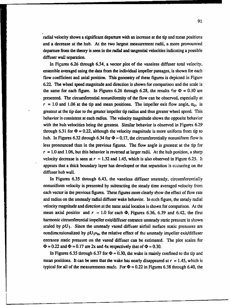
91

"radial velocity shows a significant departure with an increase at the tip and mean positions

and a decrease at the hub. At the two largest measurement radii, a more pronounced

departure from the theory is seen in the radial and tangential velocities indicating a possiblediffuser wall separation.

In Figures 6.26 through 6.34, a vector plot of the vaneless diffuser total velocity,ensemble averaged using the data from the individual impeller passages, is shown for eachflow coefficient and axial position. This geometry of these figures is depicted in Figure6.22. The wheel speed magnitude and direction is shown for comparison and the scale isthe same for each figure. In Figures 6.26 through 6.28, the results for D = 0.30 arepresented. The circumferential nonuniformity of the flow can be observed, especially atr = 1.0 and 1.06 at the tip and mean positions. The impeller exit flow angle, %0 , is

greatest at the tip due to the greater impeller tip radius and thus greater wheel speed. Thisbehavior is consistent at each radius. The velocity magnitude shows the opposite behaviorwith the hub velocities being the greatest. Similar behavior is observed in Figures 6.29through 6.31 for 0 = 0.22, although the velocity magnitude is more uniform from tip tohub. In Figures 6.32 through 6.34 for (D = 0.17, the circumferentially nonuniform flow isless pronounced than in the previous figures. The flow angle is greatest at the tip forr = 1.0 and 1.06, but this behavior is reversed at larger radii. At the hub position, a sharpvelocity decrease is seen at r = 1.32 and 1.45, which is also observed in Figure 6.25. Itappears that a thick boundary layer has developed or that separation is occurring on thediffuser hub wall.

In Figures 6.35 through 6.43, the vaneless diffuser unsteady, circumferentiallynonuniform velocity is presented by subtracting the steady time averaged velocity fromeach vector in the previous figures. These figures more clearly show the effect of flow rateand radius on the unsteady radial diffuser wake behavior. In each figure, the steady radialvelocity magnitude and direction at the same axial location is shown for comparison. At themean axial positior and r = 1.0 for each 0, Figures 6.36, 6.39 and 6.42, the first

harmonic circumferential impeller exit/diffuser entrance unsteady static pressure is shownscaled by pU1. Since the unsteady vaned diffuser airfoil surface static pressures arenondimcnsionalized by PUIvn, the relative effect of the: unsteady impeller exit/diffuserentrance static pressure on the vaned diffuser can be estimated. The plot scales for0 = 0.22 and (D = 0.17 are 2x and 4x respectively that ofN = 0.30.

In Figures 6.35 through 6.37 for 0 = 0.30, the wake is mainly confined to the tip and

mean positions. It can be seen that the wake has nearly disappeared at r = 1.45, which istypical for all of the measurements made. For 0 = 0.22 in Figures 6.38 through 6.40, the

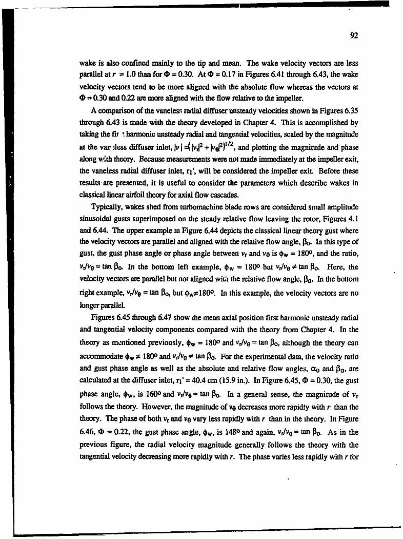
92

wake is also confined mainly to the tip and mean. The wake velocity vectors are lessparallel at r = 1.0 than for 4D = 0.30. At 4) = 0.17 in Figures 6.41 through 6.43, the wakevelocity vectors tend to be more aligned with the absolute flow whereas the vectors at) = 0.30 and 0.22 are more aligned with the flow relative to the impeller.

A comparison of the vaneless, radial diffuser unsteady velocities shown in Figures 6.35through 6.43 is made with the theory developed in Chapter 4. This is accomplished bytaking the fir + harmonic unsteady radial and tangential velocities, scaled by the magnitude

at the var -less diffuser inlet, f =( 1 J,2 + fre[)"12, and plotting the magnitude and phasealong with theory. Because measurements were not made immediately at the impeller exit,the vaneless radial diffuser inlet, rl', will be considered the impeller exit. Before theseresults are presented, it is useful to consider the parameters which describe wakes inclassical linear airfoil theory for axial flow cascades.

Typically, wakes shed from turbomachine blade rows are considered small amplitudesinusoidal gusts superimposed on the steady relative flow leaving the rotor, Figures 4.1and 6.44. The upper example m Figure 6.44 depicts the classical linear theory gust wherethe velocity vectors are parallel and aligned with the relative flow angle, N3o. In this type ofgust, the gust phase angle or phase angle between vr and vo is w = 1800, and the ratio,

v/vo = tan 13o. In the bottom left example, Ow = 1800 but vr/ve tan Po. Here, thevelocity vectors are parallel but not aligned with the relative flow angle, 0o. In the bottom

right example, vr/ve = tan P3o, but ow• 18 0o. In this example, the velocity vectors are no

longer parallel.Figures 6.45 through 6.47 show the mean axial position first harmonic unsteady radial

and tangential velocity components compared with the theory from Chapter 4. In the

theory as mentioned previously, Ow = 1800 and Vr/vo = tan P3o, although the theory can

accommodate ow * 1800 and vr/ve • tan P3o. For the experimental data, the velocity ratioand gust phase angle as well as the absolute and relative flow angles, xo and 13o, arecalculated at the diffuser inlet, rl' = 40.4 cm (15.9 in.). In Figure 6.45, 4) = 0.30, the gust

phase angle, Ow, is 1600 and vr/ve - tan IPo. In a general sense, the magnitude of Vr

follows the theory. However, the magnitude of vy decreases more rapidly with r than thetheory. The phase of both vr and ve vary less rapidly with r than in the theory. In Figure

6.46, 4d = 0.22, the gust phase angle, Ow, is 1480 and again, Vr/V0 - tan Ao. As in the

previous figure, the radial velocity magnitude generally follows the theory with thetangential velocity decreasing more rapidly with r. The phase varies less rapidly with r for

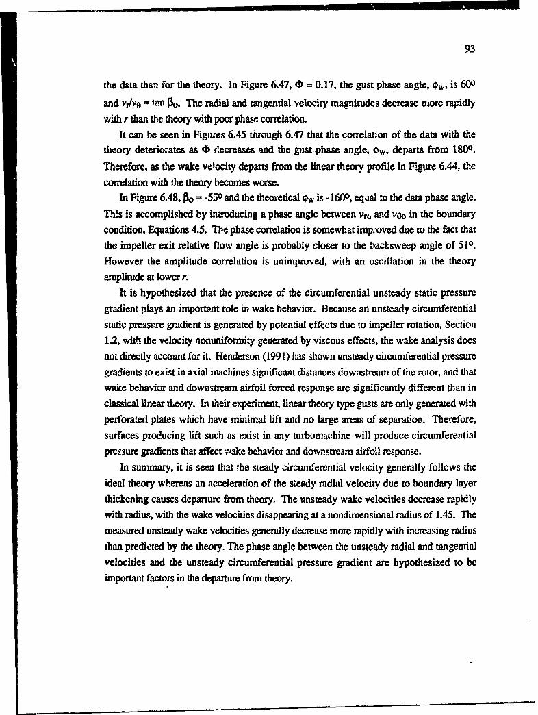
93

-the data than for tie theory. In Figure 6.47, 0 = 0.17, the gust phase angle, Ow, is 600

and v/v tan 13o. The radial and tangential velocity magnitudes decrease more rapidly

wAth r than the theory with poor phase. correlation.It can be seen in Figues 6.45 through 6.47 that the correlation of the data with the

theory deteriorates as 0 decreases and the gust phase angle, OPw, departs from 1800.

Therefore, as the wake velocity departs from the linear theory profile in Figure 6.44, the

correlation with the theory becomes worse.In Figure 6.48, 030 = -550 and the theoretical Ow is -16M°, equal to the data phase angle.

This is accomplished by introducing a phase angle between vrL, and voo in the boundary

condition, Equations 4.5. The phase correlation is somewhat improved due to the fact that

the impeller exit relative flow angle is probably closer to the backsweep angle of 510.However the amplitude correlation is unimproved, with an oscillation in the theory

amplitude at lower r.It is hypothesized that the presence of the circumferential unsteady static pressure

gradient plays an important role in wake behavior. Because an unsteady circumferential

static pressure gradient is generated by potential effects due to impeller rotation, Section1.2, with the velocity nonuniformity generated by viscous effects, the wake analysis does

not directly account for it. Henderson (1991) has shown unsteady circumferential pressure

gradients to exist in axial machines significant distances downstream of the rotor, and thatwake behavior and downstream airfoil forced response are significantly different than in

classical linear theory. In their experiment, linear theory type gusts are only generated with

perforated plates which have minimal lift and no large areas of separation. Therefore,

surfaces producing lift such as exist in any turbomachine will produce circumferential

pressure gradients that affect wake behavior and downstream airfoil response.

In summary, it is seen that the steady circumferential velocity generally follows theideal theory whereas an acceleration of the steady radial velocity due to boundary layer

thickening causes departure from theory. The unsteady wake velocities decrease rapidly

with radius, with the wake velocities disappearing at a nondimensional radius of 1.45. The

measured unsteady wake velocities generally decrease more rapidly with increasing radius

than predicted by the theory. The phase angle between the unsteady radial and tangentialvelocities and the unsteady circumferential pressure gradient are hypothesized to be

important factors in the departure from theory.

94

6.5 Diffuser Vane Unsteady Loading

Unsteady diffuser vane static pressure measurements are made at each of the geometricconfigurations listed in Table 6.1 at 0 = 0.17, 0.22 and 0.30. The unsteady lift

coefficients CL and CLs, defined in Equations 3.14 and 3.15, are presented along with thesteady lift coefficient, CL, to evaluate the diffuser vane loading as a function of diffusergeometry and flow rate. The diffuser vane surface static pressure coefficients and pressure

difference coefficients are presented along with the theory developed in Chapter 5.Figures 6.49 through 6.54 present the unsteady and steady lift coefficients, CLs and

CL, as a function of flow rate for the various diffuser geometries. The unsteady lift

coefficient CLs is the first harmonic unsteady lift amplitude nondimensionalized by thedynamic pressure based on wheel speed, Equation 3.15. This yields an absolute measure

of the vane loading as a function of the machine operating point.In Figure 6.49, the unsteady and steady lift for ri/ro = 1.10 and Nv = 30 is presented

for the various stagger angles. The unsteady lift increases markedly with 0 and withincreasing stagger, c. The steady lift changes more rapidly with 0 as a is increased, with0 L becoming more positive with increasing 4D and a.

In Figure 6.50, the radius ratio has been increased to rl/ro = 1.15. The unsteady liftchanges less rapidly with 0 and a, although the lift at 0 = 0.30 is greater for a = 600 and

700 in Figure 6.50 than for Figure 6.49. For a = 600, the unsteady lift is greater in Figure

6.50 with rl/ro = 1.15 for all 0. The increased lift at higher rl/ro is surprising since the

wake velocities are decreasing with increased radius. The steady lift behavior is similar inboth cases. It is interesting to note that the steady lift for a = 500 attains a minimum at

(D = 0.22 and further decrease in 0 and thus the negative incidence has minimal effect on

the lift. It is likely that the vaned diffuser begins to stall at this point. This behavior is

observed for all diffuser geometries.Figure 6.51 is similar to Figure 6.49 but with Nv = 15. The reduction in vane number

has a significant effect on the unsteady lift behavior. The unsteady lift is typically greaterthan for Nv = 30, however the effect of 0 on the lift is different at each value of CF. For

a = 500, the unsteady lift is greatest at high 0, for a; = 600, the unsteady lift is greatest atmoderate O,and for (a = 700, the unsteady lift is greatest at low 0. Each of these stagger

and flow rate combinations corresponds closely to the point of minimum steady incidence.The steady lift is shifted in the negative direction but shows similar behavior to the previous

figures. In Figure 6.52, the unsteady and steady lift is shown for rl/ro = 1.15 andNv = 15. Only measurements for a = 600 are made. The unsteady lift is significantly

95

reduced by increasing rl/ro to 1.15. At this radius ratio, the unsteady lift is a minimum for

minimum incidence, as opposed to a maximum as in the previous figure.In Figures 6.53 and 6.54, the effect of detuning on the unsteady lift is presented for

Nv = 30 with 40% detuning, and Nv = 10 with 13% detuning respectively. For all

measurement points, the unsteady lift is increased on one or both of the vanes. It cannot be

concluded from these cases that detuning will always produce an adverse effect on the lift,

although in general it is not always beneficial. The detuning affects the steady lift less

significantly than does the incidence.

A comparison of the unsteady airfoil surface pressure data is made with the unsteadyradial cascade airfoil theory developed in Chapter 5. The experimental diffuser vaneunsteady static pressure coefficients, Cp, are presented for both the suction and pressure

surfaces, along with the experimental and theoretical pressure difference coefficient, CAP,as defined in Chapter 3. Pressure coefficients for rl/ro = 1.15 have beennondimensionalized by the transverse velocity at ril/ro = 1.10 in order to evaluate the radius

ratio effect and since no velocity measurements are made at rl/ro = 1.15. Since the phase isdifferent at the blade leading edge than at the velocity measurement location, a phasecorrection is made. The time taken for the wave to be convected from the measurement

point to the vane leading edge is computed using the steady velocity.corrected for phase.Before making a comparison with the theory, it is useful to consider the wake velocity

profiles given in the vector plots of Figures 6.36, 6.39 and 6.42 along with the data/theorycomparison in Figures 6.45 through 6.47. In Figures 6.36 and 6.39 for 4) = 0.30 and

0.22, the wake velocity vectors are nearly parallel with the steady relative flow, andtherefore nearly transverse to the airfoils in the radial diffuser. In Figure 6.42 for(D = 0.17, the wake velocity vectors are nearly parallel with the absolute steady flow, and

therefore nearly parallel to the airfoil chord, with the transverse unsteady velocitycomponent very small. It is observed in the data/theory comparison of Figures 6.45through 6.47 that the tangential velocity component decreases with radius more rapidly thanpredicted by the theory. However, the radial component showed reasonable magnitudecorrelation in a general sense for 4D = 0.30 and 0.22. Since the radial velocity is the majorcomponent in the airfoil transverse velocity, especially at higher r, the deficiencies in theradial diffuser wake theory will not necessarily be a major source of error in the unsteadyairfoil theory.

Figures 6.55 through 6.65 present the unsteady first harmonic airfoil surface staticpressure distributions. On the lefthand axes of each figure, the amplitude and phase of the

unsteady static pressure coefficient, Cp, is plotted versus nondimensional vane chord for

96

pressure and suction surfaces. On the righthand axes, the amplitude and phase of theunsteady pressure difference coefficient, CAp, is presented along with the theory versusnondimensional chord. The legend presents the experimental and theoretical liftcoefficients, CL and CLt, as defined in Equation 3.14, along with the lift coefficient, Cis,defined in Equation 3.15.

Figures 6.55 through 6.57 show the first harmonic unsteady static pressure distributionfor 0 = 0.30, 0.22 and 0.17, respectively, with Nv = 30, rl/ro = 1.10 and ; = 600. For0 = 0.30, the amplitude of Cp is high at the leading edge for pressure and suction surfacesas is typical in steady and unsteady cascade flows. The pressure surface phase is nearlyconstant along the airfoil c., ;rd with some variation in the suction surface phase. Goodcorrelation is seen in the phase of CAp with the theory. However, the theory generallyoverpredicts the amplitude of CAp by a factor of 2 or more.

In Figure 6.56 for (D = 0.22, the amplitude of Cp is somewhat higher than in the

previous figure but the behavior is similar. The phase behavior of Cp is similar for thesuction surface but the pressure surface shows more variation. The phase correlation ofCAp has deteriorated with a greater phase decrease in the data toward the trailing edge. Thesteady flow incidence, 1, is negative for this case and positive for the previous case.Greater phase decrease at negative incidence is .een for all measurements made withNv = 30. The amplitude is closer to the theory at the airfoil trailing edge than in theprevious case. However, the theory still generally overpredicts the amplitude by a factor of2 or more.

Figure 6.57 presents the unsteady pressure for 4D = 0.17. The amplitude and phase

behavior of Cp is similar to the previous figure but the amplitude is much greater. The

phase decrease in the data for CAp occurs due to negative incidence. The amplitude of CAPis now underpredicted by the theory. TIis behavior is generally seen for all geometries at(D = 0.17, with the data greater than the theory over most of the airfoil chord. This isattributed to the small transverse wake component at (D = 0.17 which was mentionedpreviously. Since the unsteady pressure coefficients Cp and CAp are nondimensionalizedusing this transverse wake component, other effects such as incidence, airfoil geometry andimpeller circumferential pressure gradients, which are not considered in the theory, willhave a greater relative effect on the pressure distribution.

Figures 6.58 and 6.59 show the detuned cascade results for N, = 30, rj/ro = 1.10,a - 600 and 4 = 0.22. The surface pressure distributions show smoother behavior thanfor the tuned cascade, although the theory does not consider detuning. The correlation of

97

CAP with the theory is good for both vanes, with the phase slightly higher for the data than

the theory for vane 2.The correlation of the data with the theory is generally poor for the tuned cascade with

Nv = 30. This is believed to be due to the close spacing of the airfoils, thus greatlyaffecting the steady flowfield, and distorting the wake which the theory does not consider.It is hypothesized that the detuning of the cascade lessens the effect of the steady flowfield

and correlation with the theory is improved.

Figures 6.60 and 6.61 present the unsteady airfoil static pressure distribution forD = 0.30 and 0.22 respectively, with Nv = 15, rl/ro = 1.10 and ; = 600. The correlation

with theory in these cases is reasonable with some deviation in the phase correlation. Thetheory generally appears to overpredict the pressure amplitude from 10 to 25% chord for alldiffuser geometries, with this especially evident in the present figures. This is possiblyattributable to vane camber and thickness which affect the steady flow around the airfoil.The phase decrease with negative incidence no longer occurs with Nv = 15. In Figures

6.62 and 6.63, the same configuration with rl/ro = 1.15 is shown. The phase correlation isgood, with the theoretical amplitude somewhat greater than the data. This is attributable tothe unsteady pressure being noncamensionalized by the wake transverse velocity at

ri/ro = 1.10 instead of rl/ro = 1.15, where velocity data are not available.Finally, unsteady pressure data are presented for Nv = 10 in Figures 6.64 and 6.65 for

D = 0.30 and 0.22 respectively. The correlation with the theory is poor in both of these

figures. This behavior is not expected since the correlation appeared to improve withdecreasing vane number. The suction surface data for Nv = 10 matches closely the suctionsurface data for Nv = 15, however the pressure surface data is considerably different. Noexplanation is evident for this behavior.

In summary, the unsteady lift increases with flow rate 0, for Nv = 30, with this

behavior particularly noticed at higher vane stagger angles. Increasing rj/ro decreased theunsteady lift at higher 0 and a, although at lower 0, the effect is less evident. With

Nv = 15, the unsteady lift is generally greater than for Nv = 30, with less variation due toflow rate, 0. Increasing rl/ro decreased the unsteady lift significantly. Nonuniform

circumferential spacing detuning increased the lift on one or both of the vanes in all cases.Poor correlation of the unsteady pressure data with the theory was seen for Nv = 30,

with the very close vane spacing a probable cause. Reasonable correlation between dataand theory was seen with Nv = 15 at points of low vane steady loading. An unexplainable

poor correlation with theory was seen with Nv = 10.

98

6.6 Compressor InstabilitiesIn all types of pumping and compression systems, various forms of local and system

instabilities occur. Of primary relevance to gas compressors are surge and rotating stall.Surge is defined as a global instability of large mass flow oscillation through the machine atlow frequency. This can occur, as shown by Greitzer (1981), when the slope of thecompressor operating characteristic (pressure versus mass flow, as in Figures 6.1 through6.11) becomes positive. At this point, a small perturbation in system mass flow canincrease in amplitude until the flow is completely reversed in some systems, often causingcatastrophic failure.

Rotating stall is a more localized instability, in which stalling of one or more bladepassages propagates around the machine circumference at some fraction of the wheelspeed, typically 20 to 70% according to Greitzer (1981). Stability analyses for rotatingstall are generally more complicated and less exact than for surge, with precise a prioriprediction of a compressor stall point difficult to obtain. However, rotating stall isgenerally observed around the zero slope portion of the compressor operatingcharacteristic, with stalling more severe as the flow rate is decreased. Rotating stall issometimes observed on the negatively sloped portion of the compressor operatingcharacteristic, especially in high speed, multi-stage axial compressors. Non-stalledoperation on the positive portion of the characteristic is rare.

The classic explanation of rotating stall onset is given by Emmons, et al. (1955). Whena turbomachine blade row is operating at high incidence angle, a disturbance in the flow canlocally increase this angle, stalling one of the blades, As this blade stalls, the flow throughthe stalled passage is diverted into the adjacent passages, decreasing the incidence on one,while increasing the incidence on the other, thus causing it to stall. This sequence repeatsitself, causing the stall cell to rotate around the machine. More recent studies have shownstall to develop from small amplitude rotating waves which can increase in amplitude atcertain machine operating points. It has been observed in the literature (Van denBraembussche, 1984) and also in the present investigation, that localized or global bladestalling is not always a sufficient condition for rotating stall.

Surge and rotating stall are distinct phenomena. However, they are not unrelated.Occurrence of rotating stall can often trigger the global instability of surge in axialcompressors. Although much effort has been made to predict and reduce these phenomenain turbomachines, their occurrence and behavior is still not well understood, especially incentrifugal compressors. In this regard, occurrence of system instabilities in the Purdue

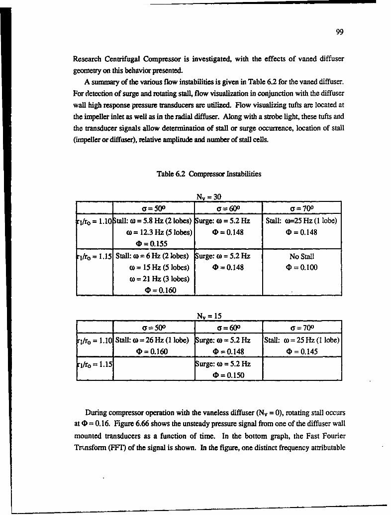
99

Research Centrifugal Compressor is investigated, with the effects of vaned diffuser

geometry on this behavior presented.A summary of the various flow instabilities is given in Table 6.2 for the vaned diffuser.

For detection of surge and rotating stall, flow visualization in conjunction with the diffuserwall high response pressure transducers are utilized. Flow visualizing tufts are located atthe impeller inlet as well as in the radial diffuser. Along with a strobe light, these tufts and

the transducer signals allow determination of stall or surge occurrence, location of stall

(impeller or diffuser), relative amplitude and number of stall cells.

Table 6.2 Compressor Instabilities

Nv =30

a =500 a=600 a=700

rl/ro = 1.10 Stall: (o = 5.8 Hz (2 lobes) Surge: o) = 5.2 Hz Stall: o0=25 Hz (1 lobe)oo= 12.3 Hz (5 lobes) D=0.148 D=0.148

0 = 0.155

ri/ro = 1.15 Stall: co = 6 Hz (2 lobes) Surge: o) = 5.2 Hz No Stalla = 15 Hz (5 lobes) 0=0.148 D=0.100

co = 21 Hz (3 lobes)

(D = 0.160

_ _ _Nv = 15

o=500 a= 600 =700

rl/ro= 1.10 Stall: 0 = 26 Hz (l lobe) Surge: o=5.2Hz Stall: co=25Hz(I lobe)D = 0.160 0 = 0.148 0 = 0.145

rl/ro = 1.15 Surge: co = 5.2 Hz

I_ _ (D = 0.150

During compressor operation with the vaneless diffuser (Nv = 0), rotating stall occursat 0 = 0.16. Figure 6.66 shows the unsteady pressure signal from one of the diffuser wall

mounted transducers as a function of time. In the bottom graph, the Fast Fourier

Trainsform (FFT) of the signal is shown. In the figure, one distinct frequency attributable

100

to rotating stall is seen at (o = 26 Hz. This frequency decreases slightly as (D is reduced.

The tufts at the impeller inlet and exit respond to the stall cell, which appears to originate in

the impeller. At all times during stall, only one stall cell is observed (inferred from thephase angle between the transducer signals). The machine is operated to CD 0.12, with

the single cell impeller stall the only instability observed.For vaned diffuser operation, several types of instability are observed. The frequency

given in Table 2 is the cell passing frequency. Therefore, a stall pattern at a) = 5.8 Hz with

2 cells is a 2-celled pattern rotating at 2.9 Hz. The impeller rotational speed is 29.8 Hz,therefore the stall frequency is approximately 20% of the impeller frequency. When severalfrequencies are present, some of the harmonics can add or subtract to yield other

harmomcs.

The first half of Table 6.2 show results with Nv = 30. In the first row, flowinstabilities with rilro = 1.10 are listed. For o = 500, the diffuser stall contains two distinctfrequencies and number of cells. The stall at W = 5.8 Hz appears to be surge during

operation. However, the transducer phase content suggests that it is stall. Since rotatingstall can trigger surge, it is likely that this stall frequency will produce surge at lower flowrates. For u = 600, surge occurs at C = 0.148. The transducer signal is shown in Figure

6.67. The single surge frequency around w = 5 Hz is seen. The phase difference between

the transducers is close to zero, indicating the global mass flow oscillation. No rotatingstall patterns are observed before surge. For a = 700, a stall develops which is similar to

the vaneless diffuser impeller stall. However, minimal tuft movement is observed at theimpeller inlet as opposed to the vaneless case thus the location of this stall is uncertain.

The behavior for rl/ro = 1.15 is given in the second row of Table 6.2. Figure 6.68presents the trarisducer signal and FFT for a = 500. Three distinct frequencies are %.videntat w = 6, 15 and 21 Hz, with the apparent number of stall cells being 2, 5 and 3

respectively. It is possible that 2 patterns exist and that their sum or difference producesthe third frequr .cy. For a = 600, the behavior is similar to ri/ro = 1.10, with surgeoccurring. For a = 700, no instabilities are observed operating the machine to 4) = 0.10.For Nv = 15, impeller stall occurs at a = 500 and 700. The flow coefficient for Y = 700 islower, (D = 0.145, than for the vaneless impeller stall where (D = 0.160. For a = 600,

surge occurs as in the previous cases.

The vaned diffuser is seen t,. have a significant influence on the occurrence ofcompressor instabilities. The flow coefficient for stall can be reduced by proper geometryselection. For Nv - 30, a = 700 and rl/ro = 1.15, stall and surge behavior are completely

eliminated, thus giving support to the belief that rotating disturbances will only be amplified

101

under certain conditions, with static stalling of individual blades or vanes not always

sufficient.

102

1.4.Impeller

---- Stage

• "1.2 -

1.0- % %

V S

Nv =00.8.

1.0-

SO0.9-

0.8-"

S%SN

0.70.15 0.20 0.25 0.30 0.35

Flow Coefficient, 0

Figure 6. 1. Centrifugal Compressor Performance with Vaneless Diffuser

.. •~m mMIW~n~m W~m Bwmmi Nii~mm mmmum J t .. ...... TS

S ii i i l i mlllmi l ul mlnlS

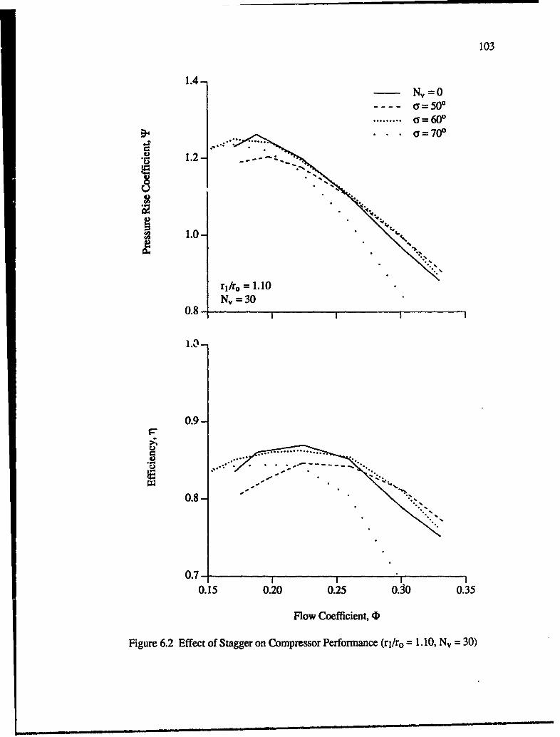
103

1.4-N =0

---- a=50'

......... c=60

•1.2 -

1.0-

rllr. - 1.10N= 30

0.8

1.3-

0.9-

0.8-

0.7-

0.15 0.20 0.25 O0O 0.35

Flow Coefficient, 4

Figure 6.2 Effect of Stagger on Compressor Performance (rj/ro = 1.10, Nv = 30)

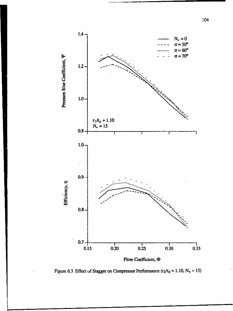
104

1.4-N,,=0a a=50P

*......... a=60°a=701

•1.2 - - - - . . ..

1.0-

rl/r0 =1.10N,, =15

0.8 I I

1.0-

0.9-,• ~ ~. .. ;.......... ...

0.8-

0.7-0.15 0.20 0.25 0.30 0.35

Flow Coefficient, (D

Figure 6.3 Effect uf Stagger on Compressor Performance (rl/ro = 1.10, Nv = 15)

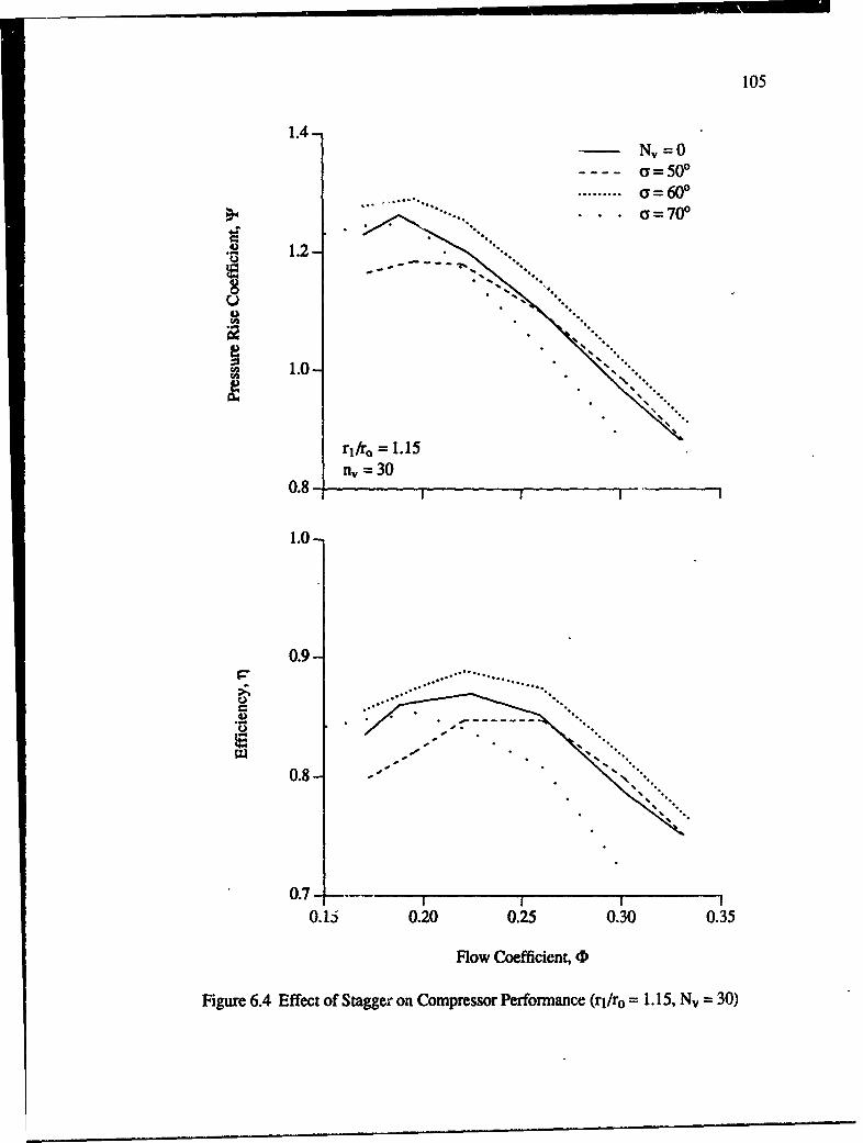
105

1.4-Nv=0

- --- a=50°S........ a= 60°

... ~~~~ -... 70'

1.2-

1.04

rtfr0 = 1.15n= 30

0.8-

1.0-

F 0.9-

0.8-

0.7/ 0.--- I I II

0.15 0.20 0.25 0.30 0.35

Flow Coefficient, (D

Figure 6.4 Effect of Stagger on Compressor Performance (rl/ro = 1.15, Nv = 30)

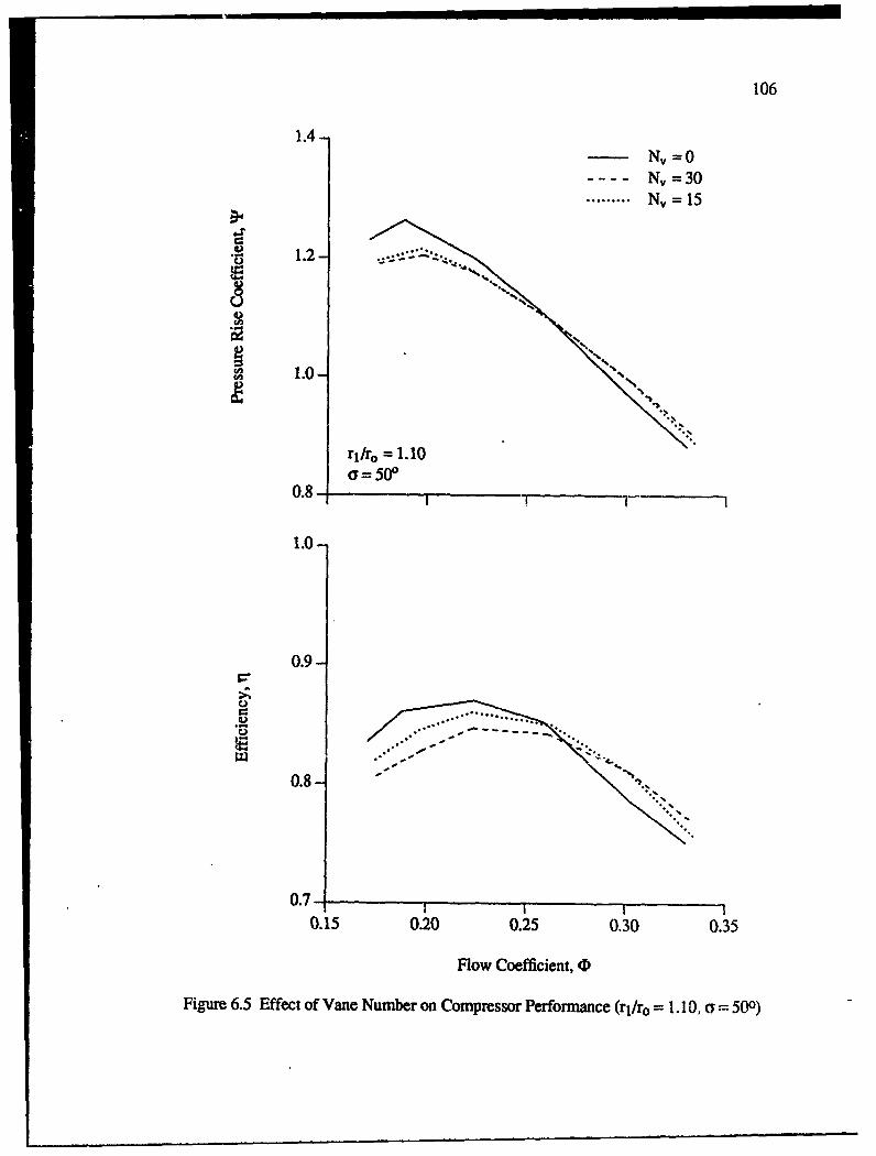
106

1.4-Nv=0-N =30

......... Nv = 15

1.2-

U9,

1 1.0-

rl/ro = 1.10a=50'

0.8

1.0-

0.9-

0.8 - '.

0.7

0.15 0.20 0.25 0.30 0.35

Flow Coefficient, (D

Figure 6.5 Effect of Vane Number on Compressor Performance (rl/ro = 1. 10, c = 500)

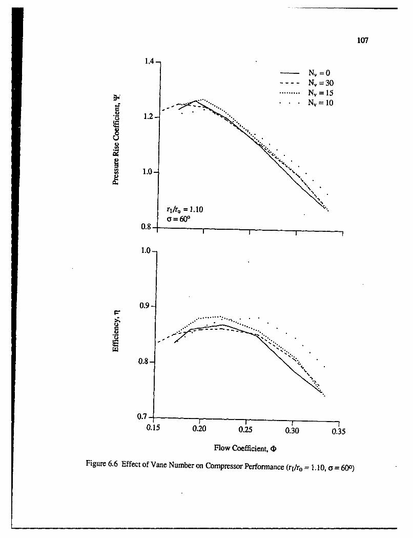
107

1.4-

Nv =0N, = 30

......... N, = 15

. N,=10

1.-.

O= 6000.8 -

1.0-

0.9-

0.8-

0.7I I0.15 0.20 0.25 0.30 0.35

Flow Coefficient, (DFigure 6.6 Effect of Vane Number on Compressor Performance (rl/ro = 1.10, a = 60")

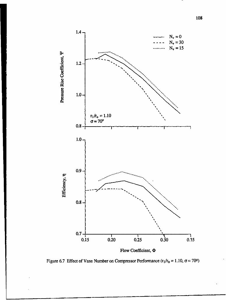
108

1.4-Nv =0N, = 30

......... Nv = 15

• 1.2-

\%°,

1.0-

1lr 1..0S~ri/i*o = 1.10 ,

0= 70°0.8-

1.0-

0 0.9-

0.8-

0.7-0.15 0.20 0.25 0.30 0.35

Flow Coefficient, 0

Figure 6.7 Effect of Vane Number on Compressor Performance (r1/ro 1. 10, a = 700)

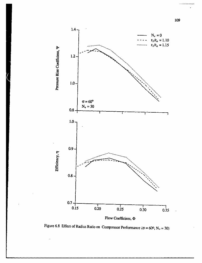
109

1.4-

N =0.--- rl/ro = 1.10

.................... •......... r, /ro = 1. 15

"1.2-

1.0-

a= 0Nv=30

0.8 - _ _ _ _ _ _ _ _ _ _ _ _ _ _ _ _ _ _ _ _ _

1.0-

0.9-

0.8-

I i I

0.79-

0.15 0.20 0.25 0.30 0.35

Flow Coefficient, (DFigure 6.8 Effect of Radius Ratio on Compressor Performance (a = 600, N, = 30)

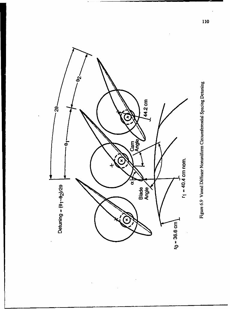
110

E C

C4

00

E

CDC

CD))

CM C)

o >

C

co0 0)

11I

1.4-

Nv=0- --- Tuned......... 40% Detuned

Z • 1.2-

1.0-

r•/ro 1.10T = 600

N=300.8

1.0-

0.9-

......... ... ..F'".

0.8-

0.7 1

0.15 0.20 0.25 0.30 0.35

Flow Coefficient, 0Figure 6.10 Detuned Diffuser Compressor Performance (rj/ro = 1.10, a = 600, Nv = 30)

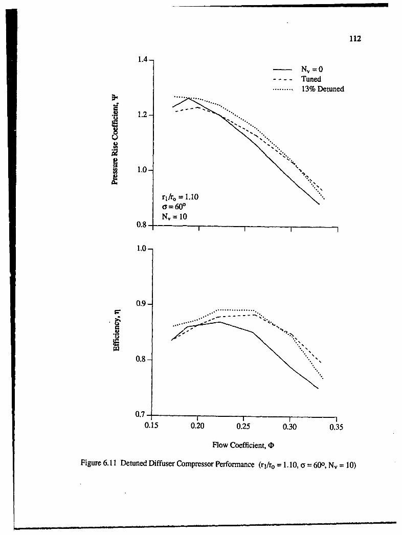
112

1.4-N=0

- - -- Tuned

.....13% Detuned

1.0-

rlfr. 1.10

0.8 N,1

1.0-

0.9-

0.8-

0.7-0.15 0.20 0.25 0.30 0.35

Plow Coefficient, 0

Figure 6.11 Detuned Diffuser Compressor Performance (r11ro 1. 10, a Y 600, Nv 10)

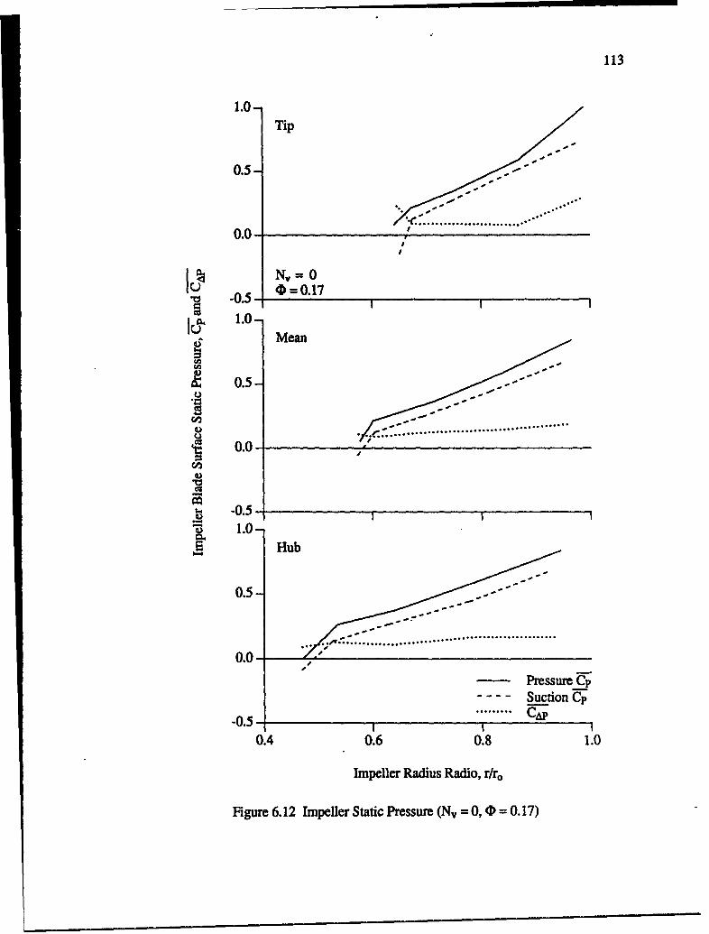
113

1.0-Tip

0.5-

0.0- I"

I

I -0.5 (D-=o.171.0-

Mean

0.5-

,• 0.0 - J.

S-0.5"Z 1.0-Hb

0.5-

0.0-

Pressure C-- - Suction Cpp

-0.5 .. I....... CAP

-0.5-

0.4 0.6 0.8 1.0

Impeller Radius Radio, r/to

Figure 6.12 Impeller Static Pressure (Nv = 0, 0 = 0. 17)S•- --- Suction C•

114

1.0-

Tip

0.5-

0.0-

• • - ~0. = 0.22

0.5-

J 0.0..

1.0-Hub

0.5-

0.0-

Pressure Cp---- Suction Ep

.... .... ......... CAP-0.5-I

0.4 0.6 0.8. 1.0

Impeller Radius Radio, r/ro

Figure 6.13 Impeller Static Pressure (Nv = 0, (D = 0.22)

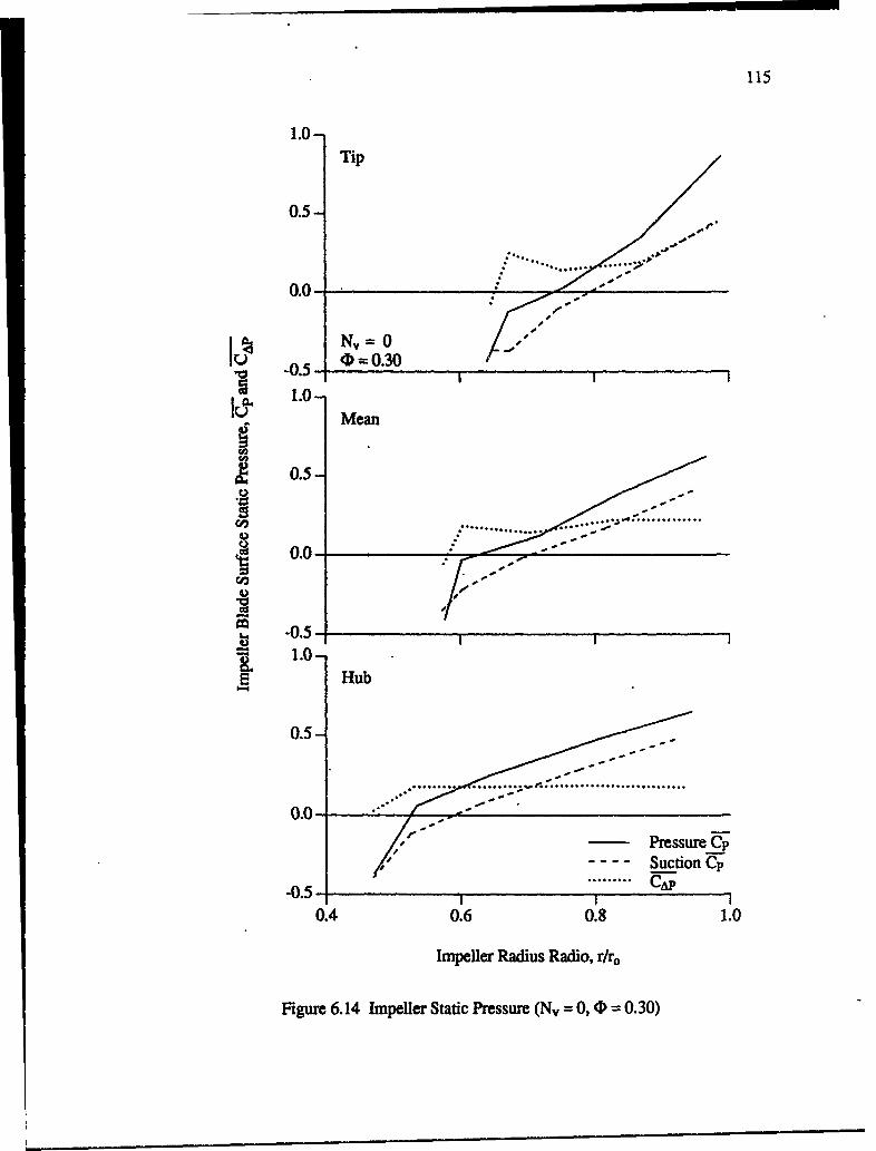
1.0-Tip

0.5-

* ...... ...

0.0- .

-v 0

.~-0.5- D03

1.0-6 Mean

0.5-

U2....................................~..............

J 0.0-

14 -0.5-

1.0-

2 Hub

0.5-

........ ....... ......r........................0.0- - /U-

Pressure Cp- - -- Suction Cp

-0.5-. ... A

0.4 0.6 0.8 1.0

Impeller Radius Radio, r/r,0

Figure 6.14 Impeller Static Pressure (Nv = 0, CID = 0.30)

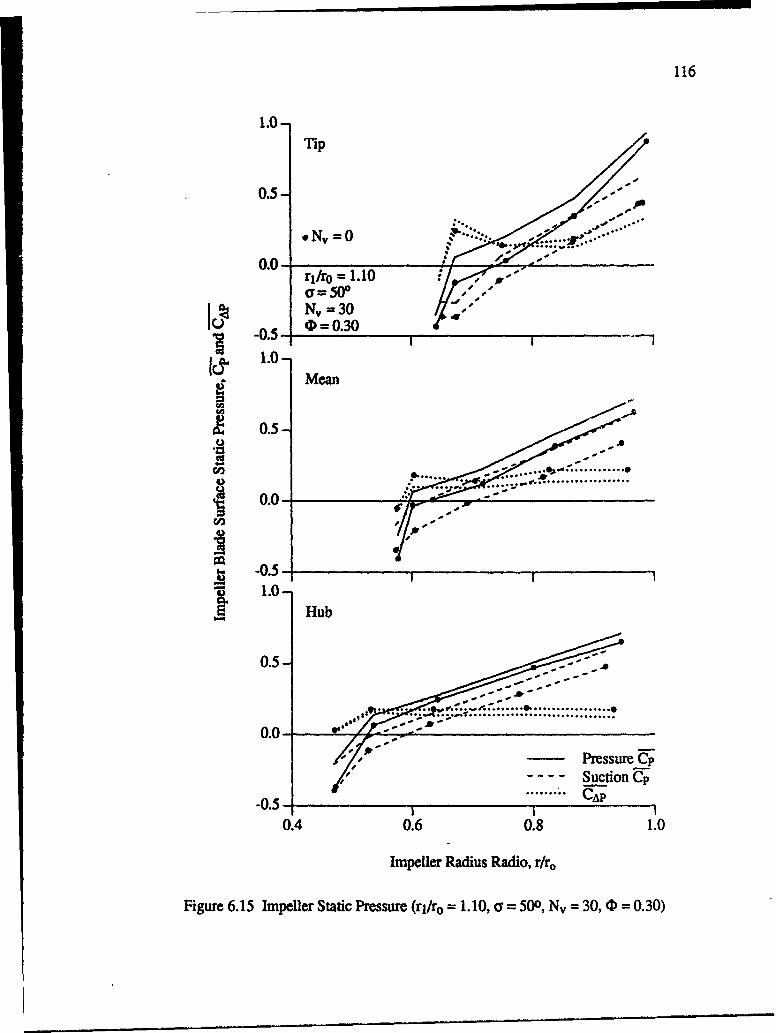
116

1.0-Tip

0.5--

0.0-

'~-0.5- 0 =.3

1.06 Mean

0.5-A

- ..-......

V.. ...........

-0.5-

0.0--

-0.5-

1.0-

-0. .............

0.4 0.6 0.8 1.0

Impeller Radius Radio, r/r.

Figure 6.15 Impeller Static Pressure (rj/r0 = 1. 10, a = 500, Nv, = 30,4)D = 0.30)

117

1.0-Tip

0.5-

. Nv =0

0.0-rl/ro = 1.10 -

a =60PNv =30-o = 00.22

1.0-Mean

1.

0.5-

0.0-

-0.5-1.0-

E Hub

0.5-e

...................

Pressure Cp--- uction Cp

-0.5- ..... A

0.4 0.6 0.8 1.0

Impeller Radius Radio, r/r.

Figure 6.16 Impeller Static Pressure (rl/ro = 1. 10, aF = 600, Nv = 30, 4D) 0.22)

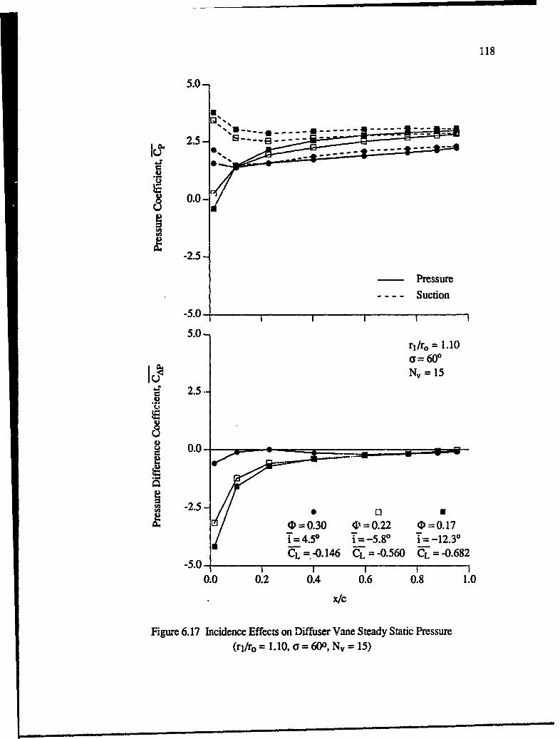
118

5.0-

-2.5-

5.0

-2.5-

-50

5.0

~ 2.5-

0 0.30 4% 0.22 (D 0. 17..45O i-5.9, i-12.3'

-5.0 ýýQ=-0.146 EL -0. 5 6 0 6L= -0. 6 8 2

0.0 0.2 0.4 0.6 0.8 1.0

x/C

Figure 6.17 Incidence Effects on Diffuser Vane Steady Static Pressure(rl/ro 1.10, ar= 600, Nv = 15)

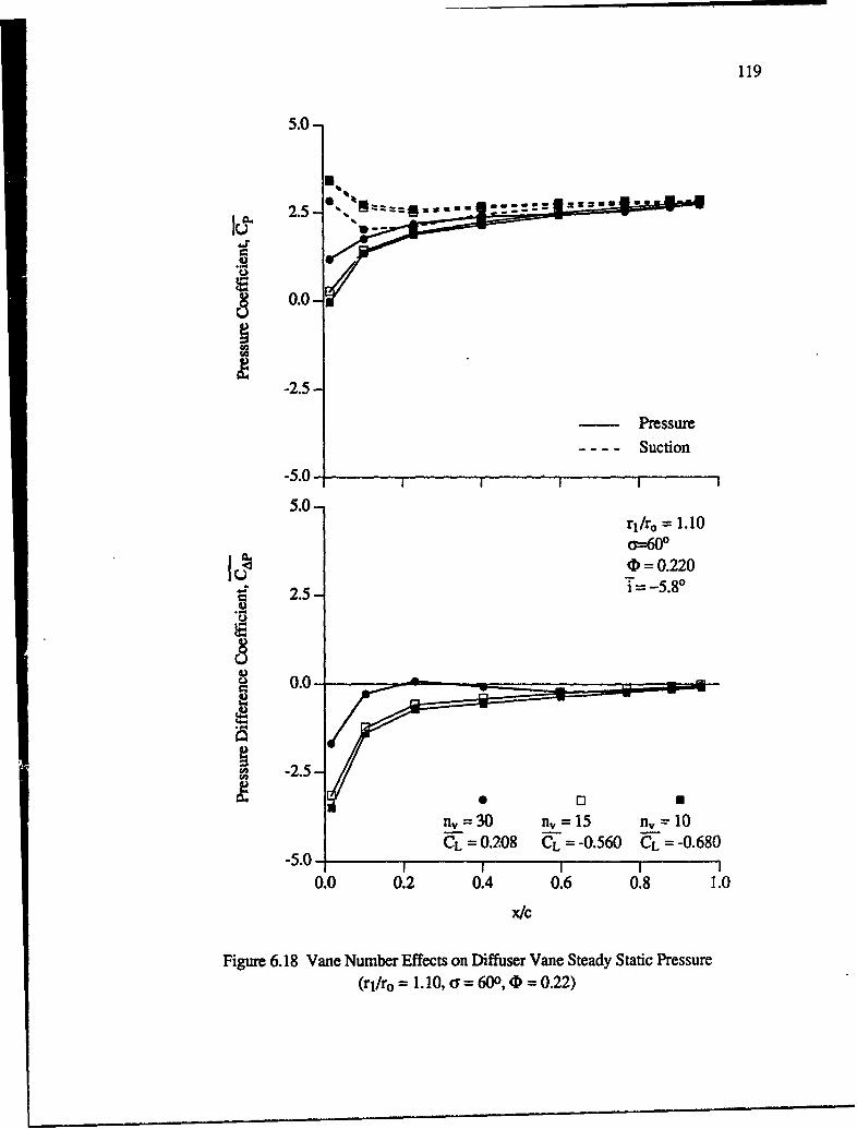
119

5.0-

2.5 -' ' !! =,...

0.0-

-2.5-

Pressure---- Suction

-5.0

5.0-r1/ro = 1.10a=600

0 =0.220.= -5.80

2.5-

0.0-

2.5-•, -2.5-

nv =30 nv =15 nv -10-LL = 0.208 EL =-0.560 CLL :-0.680

-5.0-

0.0 0.2 0.4 0.6 0.8 1.0

x/c

Figure 6.18 Vane Number Effects on Diffuser Vane Steady Static Pressure(rl/ro = 1.10, cr= 600, 0 = 0.22)

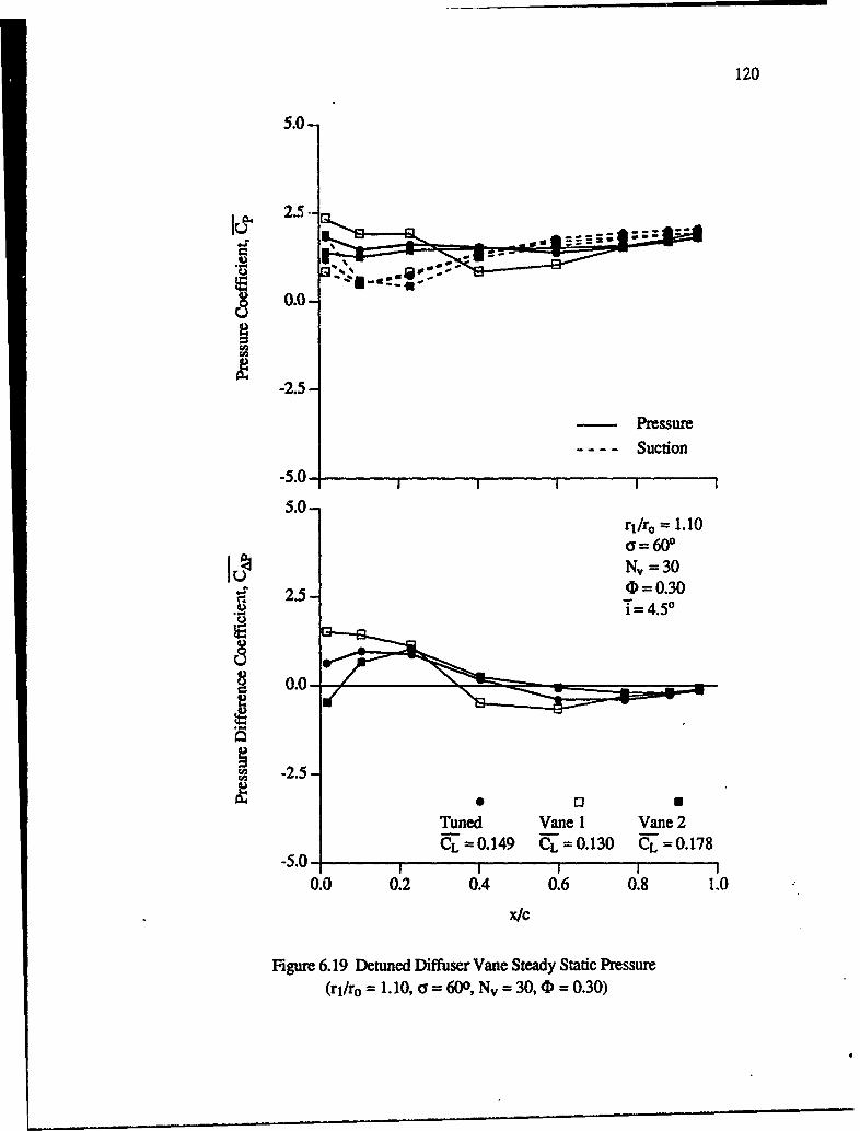
120

5.0-

-2.5-

Pressure---- Suction

5.0 II

r1/r0, = 1.10a=600N,=30

a 2.5(D) = 0.30

0.0-'44

r, 2.5-

0 U3

Tuned Vane 1 Vane 2

-5.0 CL = 0. 149 6L= 0.130 CL =0.178-50 IIII0.0 0.2 0.4 0.6 0.8 1.0

x/c

Figure 6.19 Detuned Diffuser Vane Steady Static Pressure(ri/ro = 1. 10, cr = 600, Nv = 30, (D = 0.30)

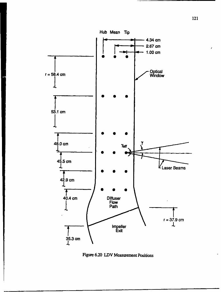
121

Hub Mean Tip

. 4.34 cm2.67 cm1.00 cm

Ir = 58.4 cm Window

53.1 cm

48.0 cmI4 * . * - -.----

45.5 cm1.. Laser Beams

42.9 cm

40.4 cm DiffuserFlow2.. Path

r =37.9 cm

35.3 cm

4aFigure 6.20 LDV Measurement Positions

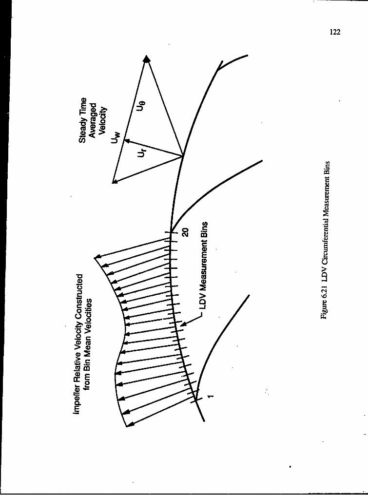
122

0

CM'

0C-4

2:0

0a

.> cc E

r.

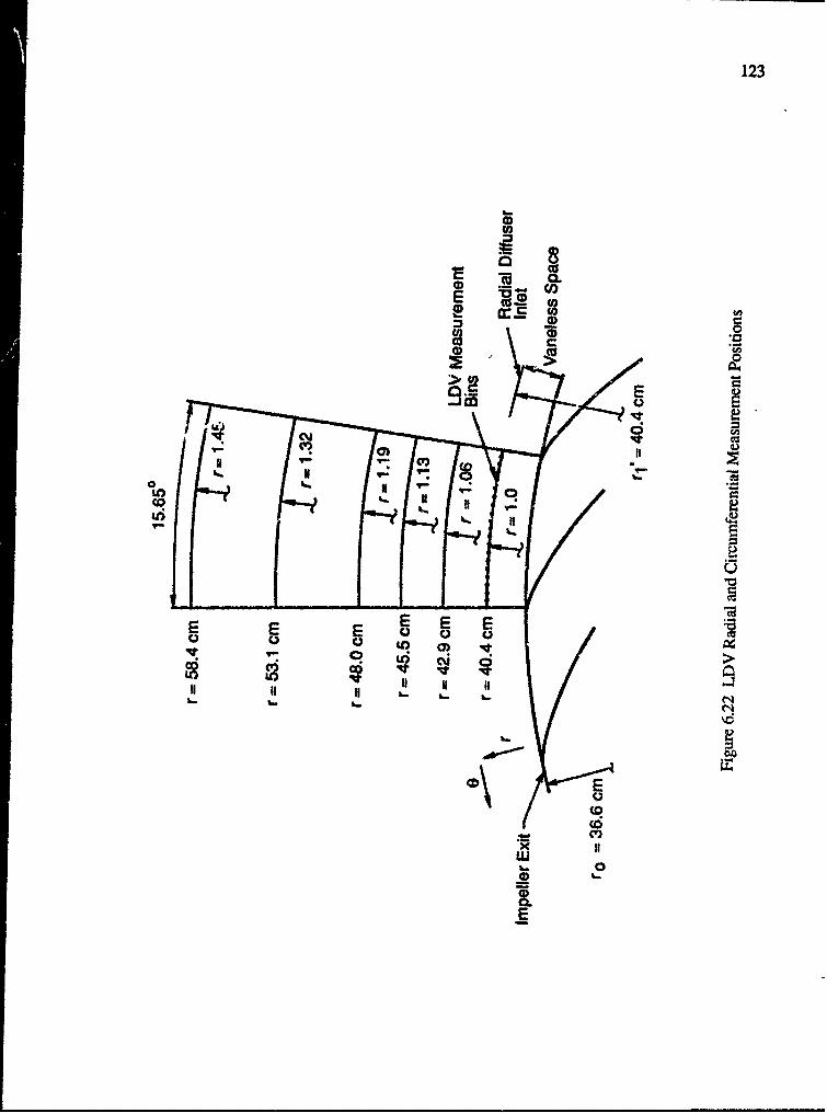
123

0 c

EE02

a *caL()l

(O0

E E EE0 0 0

0 id H

L.00

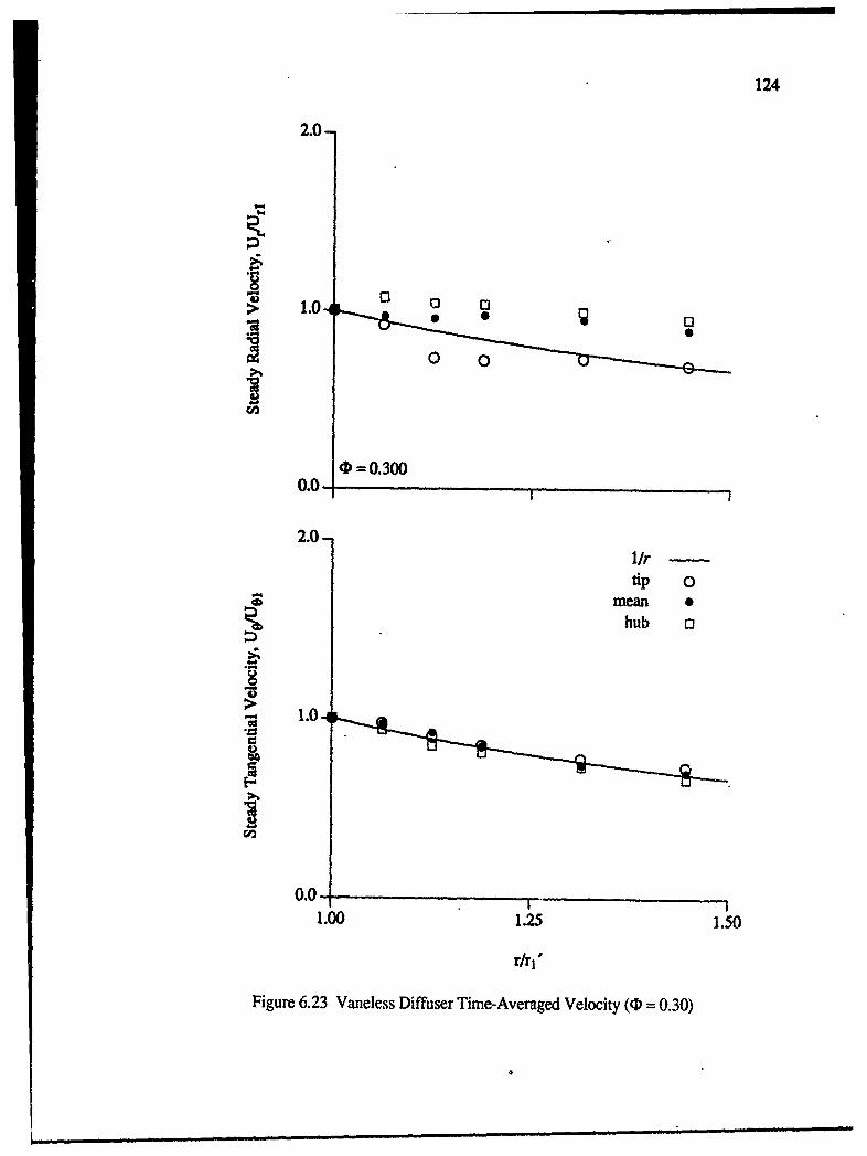
124

2.0-

0 0

0.00

'1 0

0.0. _ [( 0.0

2.0-Ur-tip 0

mean *hub o

1. .

C,,

0.0-1.00 1.25 1.50

r/r, 1

Figure 6.23 Vaneless Diffuser Time-Averaged Velocity (0 -0.30)

i]1 Jl llm lllll llllllll~ lI~ll _i _1 ] [ [Il~mll __ J ! II IT JJ [ [ l . .. . m T I IF T • II I. .. ... .. ... .. . ..

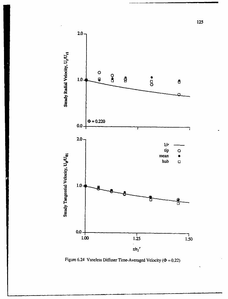
I 125

2.0-

S00

D -0.2200.0

2.0-h1r -tip 0

.Wmean *hub a

*~ 1.0

0.0 -11.00 1.25 1.50

r/r1

Figure 6.24 Vaneless Diffuser Time-Averaged Velocity (D = 0.22)

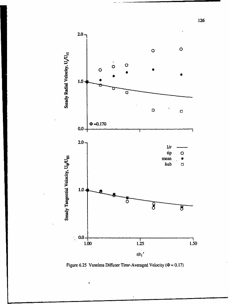
126

2.0-

0 0

0 0

•=.1700.0-4

2.0-lr -tip 0

0 mean 0hub o

0.0-1.00 1.25 1.50

Figure 6.25 Vaneless Diffuser Time-Averaged Velocity (D = 0.17)

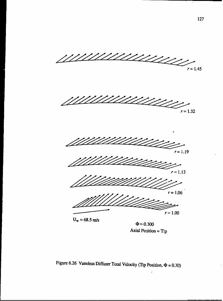
127

r= 1.19

r= 1.13

U, 68.5 ni/s

Axial Position =Tip

Figure 6.26 Vaneless Diffuser Total Velocity (Tip Position, 0b = 0.30)

128

dZ~r=1.32

Axial ositio=1.Mea

Figre6.2 VneessDifuer otl Vloit (ManPoitn,( r=10.130

129

r-=1.45

r = 1.06

---.- - -- '- ' " -r r = 1.0 0

Uw= 68.5 rn/s= 0.300

Axial Position = Hub

Figure 6.28 Vaneless Diffuser Total Velocity (Hub Position, 4, = 0.30)

130

r= 1.13

r= 1.06

Uw~ 68.6 ni/s(D 0.220

Axial Position =Tip

Figure 6.29 Vaneless Diffuser Total Velocity (Tip Position, (D) = 0.22)

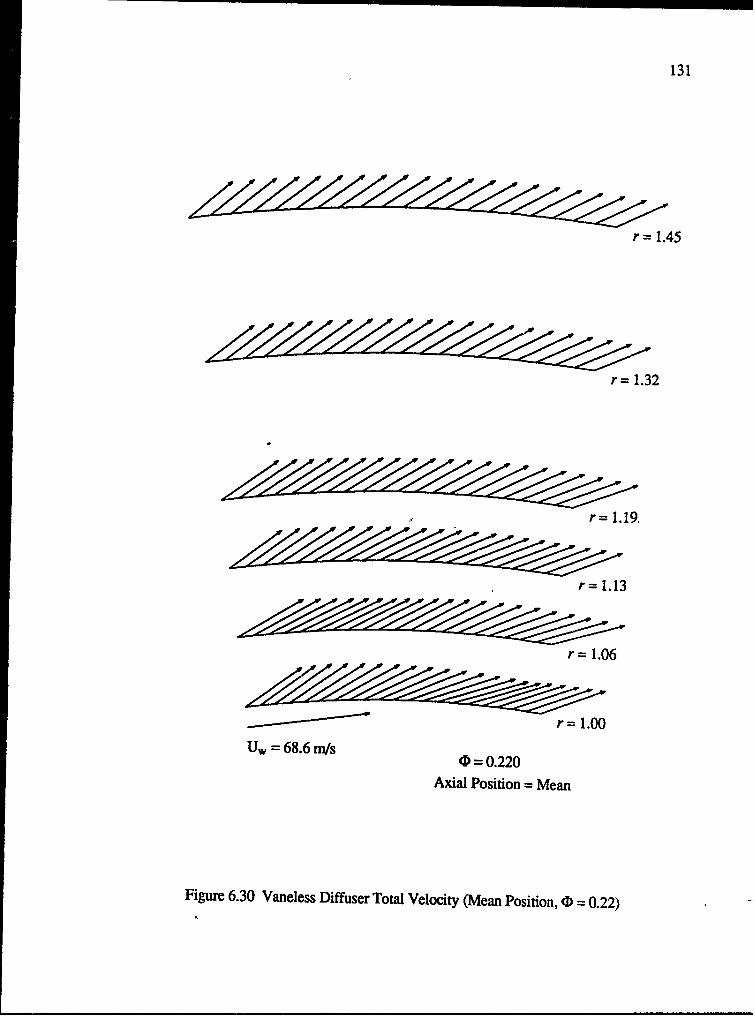
131

U~ 6r=1.45

cIr=1.32

Axial ositio1.1Mea

Figre6.3 VneessDifuer otl Vloit (ManPoitn,'r=10.22)

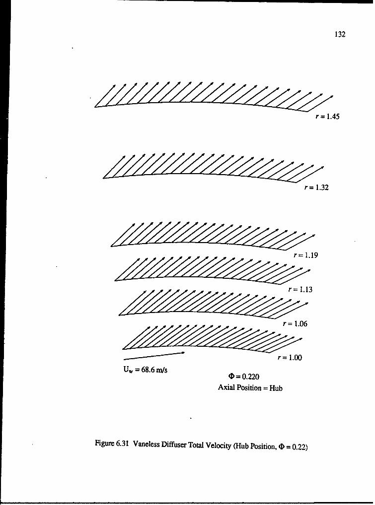
132

=~ 68. 1.45

Axial ~ ~ r P1it.32 u

Figre .31Vanles Dffuer otl Vlocty Hu Poitin, I r= 0.22)

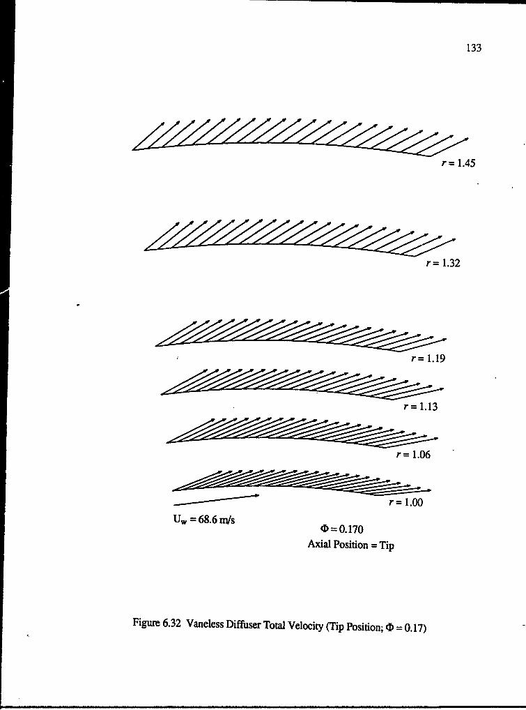
133

cIr=1.13

Axial Position =Tip

Figure 6.32 Vaneless Diffuser Total Velocity (Tip Position; (I) = 0. 17)

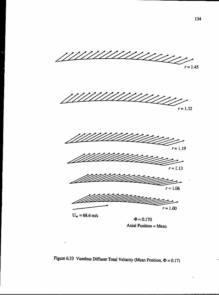
134

r= 1.13

=~ 68. 1.06

U, 68. m/s 0. 170Axial Position =Mean

Figure 6.33 Vaneless Diffuser Total Velocity (Mean Position, (D = 0. 17)

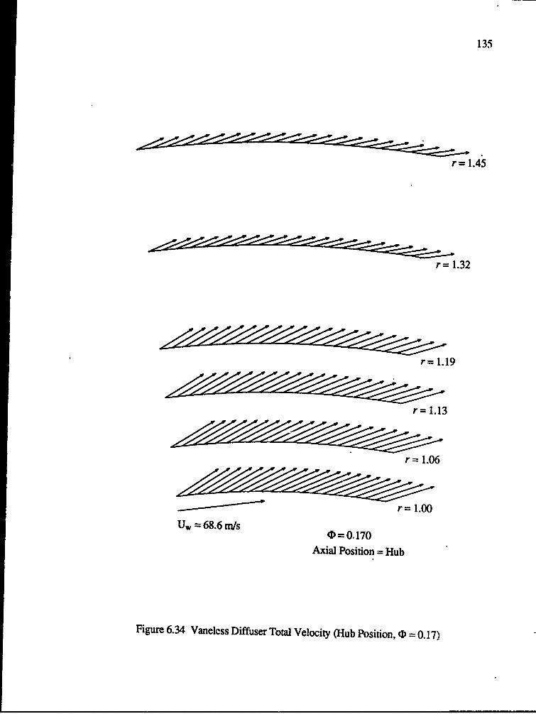
135

=~ 68. 1.45

4r=O1.19

Axial Position =Hub

Figure 6.34 Vanelcss Diffuser Total Velocity (Hub Position, (D = 0. 17)

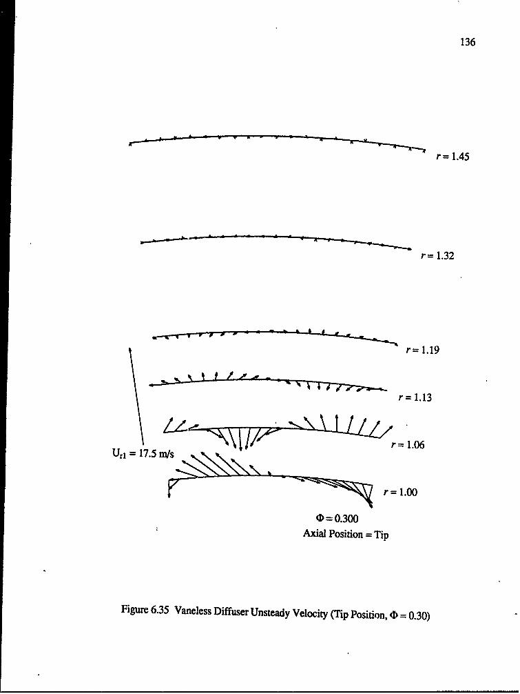
136

r = 1.45

r = 1.32

r= 1.19

r= 1.13

r=1O

r 1.00

(- 0.300Axial Position = Tip

Figure 6.35 Vaneless Diffuser Unsteady Velocity (Tip Position, (D = 0.30)

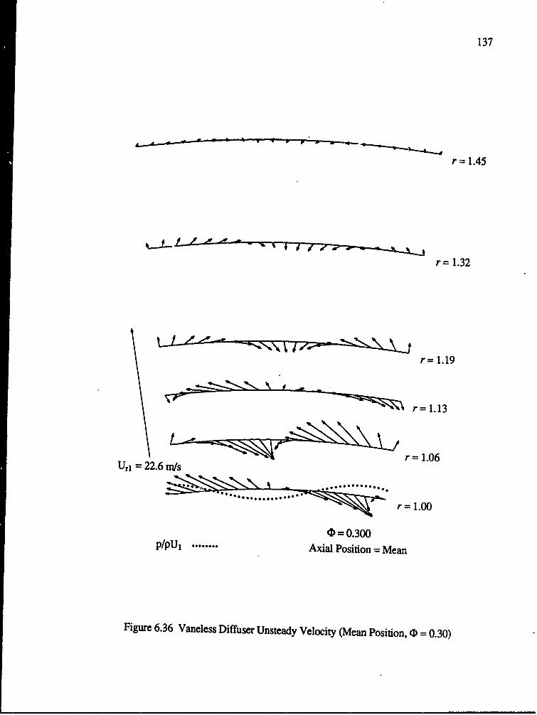
137

p,-- " • .- A r p -..

r = 1.45

r = 1.32

r= 1.19

r= 1.13

Uri- 22.6 s1.06

r= 1.00

(D = 0.300p/pU1 ........ Axial Position = Mean

Figure 6.36 Vaneless Diffuser Unsteady Velocity (Mean Position, (D = 0.30)

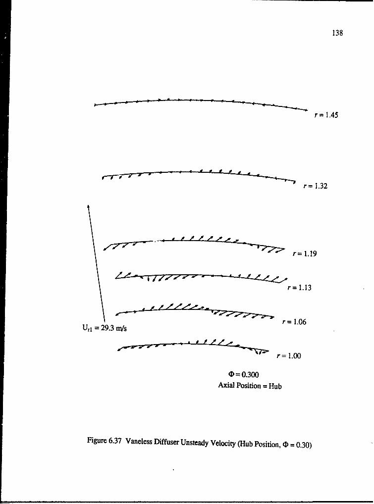
138

r= 1.45

r= 1.32

r= 1.19

r= 1.13

r = 1.06Ul 1 29.3 m/s

r = 1.00

(D 0.300

Axial Position = Hub

Figure 6.37 Vaneless Diffuser Unsteady Velocity (Hub Position, (D = 0.30)

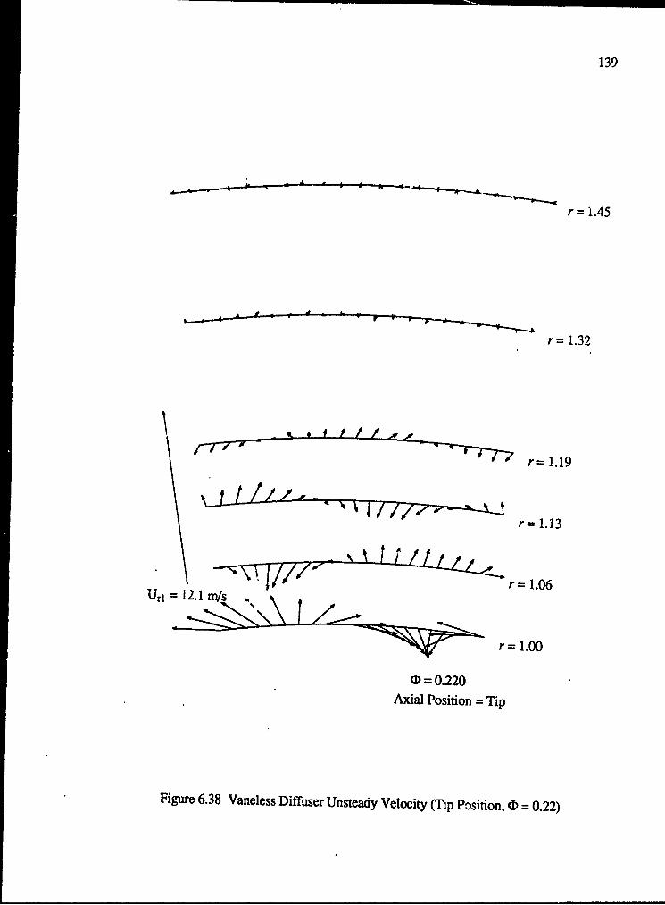
139

r = 1.45

r= 1.32

r= 1.19

r= 1.13

r = 1.06Uri=12.1m/ n • •

r= 1.00

(= 0.220Axial Position = Tip

Figure 6.38 Vaneless Diffuser Unsteady Velocity (Tip Position, (D = 0.22)

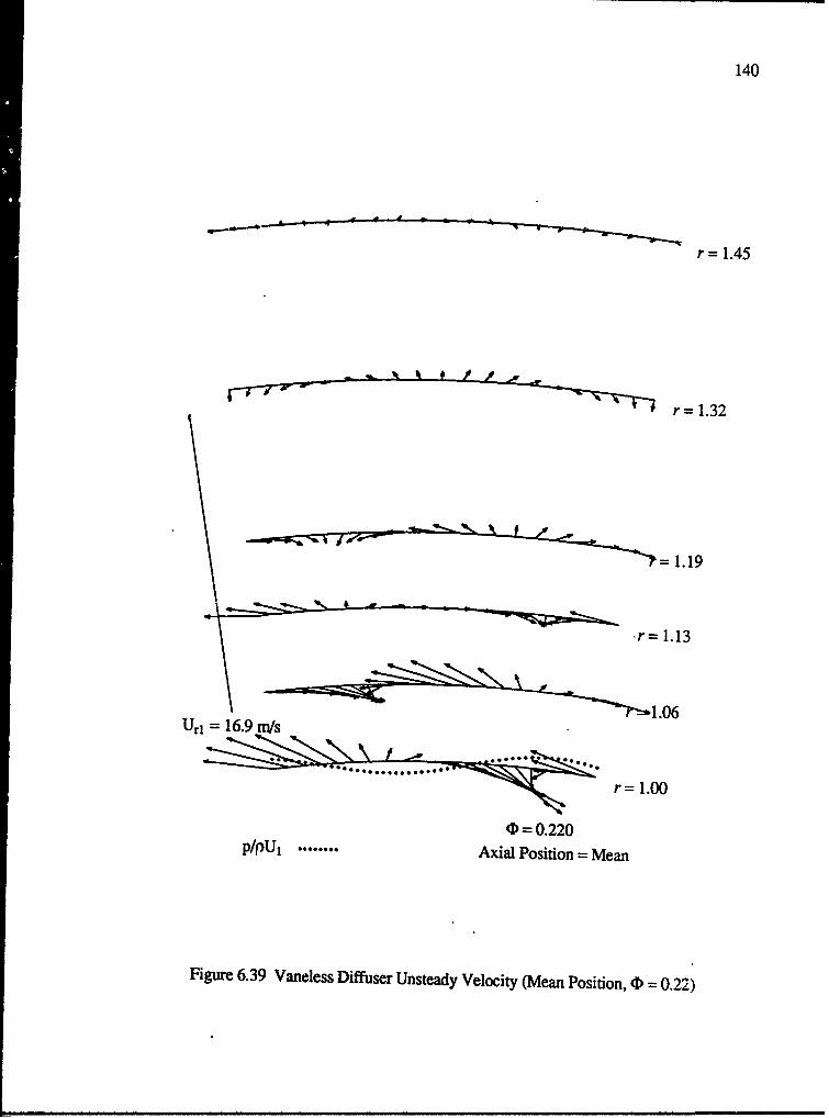
140

r = 1.45

r= 1.32

=1. 19

Uri= 16.9 rn/s

r= 1.00

(D 0.220p/p)Ui.... Axial Position =Mean

Figure 6.39 Vaneless Diffuser Unsteady Velocity (Mean Position, (D = 0.22)

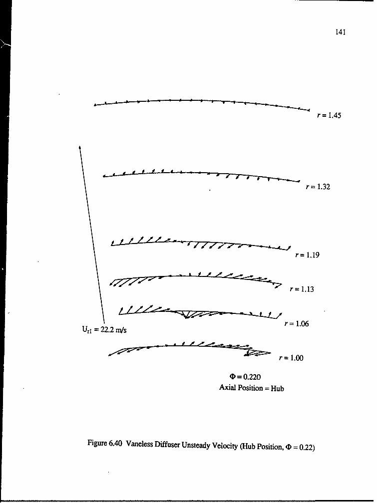
141

r= 1.45

r = 1.32

r= 1.19

r= 1.13

S2 1.06Urn = 22.2 mi/s

r= 1.00

D= 0.220

Axial Position = Hub

Figure 6.40 Vaneless Diffuser Unsteady Velocity (Hub Position, (D = 0.22)

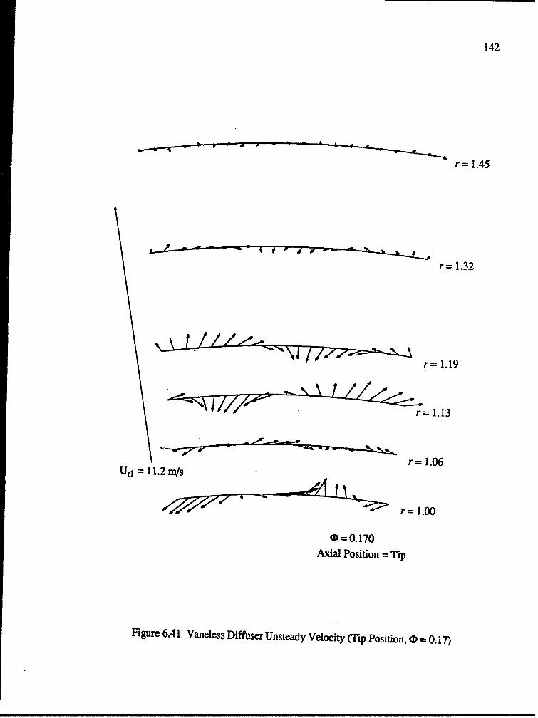
142

r = 1.45

r= 1.32

r= 1.19

r = 1.06

r = 1.00

0, 0. 170Axial Position =Tip

Figure 6.41 Vaneless Diffuser Unsteady Velocity (Tip Position, 4, = 0. 17)

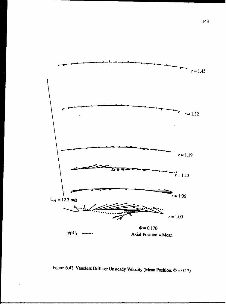
143

r = 1.45

r= 1.32

r= 1.19

r= 1.13

S1. r= 1.06

r= 1.00

(D=0.170p/pU1 ........ Axial Position = Mean

Figure 6.42 Vaneless Diffuser Unsteady Velocity (Mean Position, (D = 0.17)

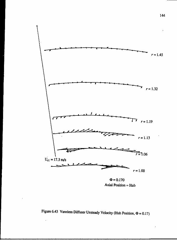
144

r = 1.45

r= 1.32

r= 1.19

r= 1.13

S~.06

Uri 17.3 m/s

r= 1.00

(D=0.170

Axial Position = Hub

Figure 6.43 Vaneless Diffuser Unsteady Velocity (Hub Position, (D = 0.17)

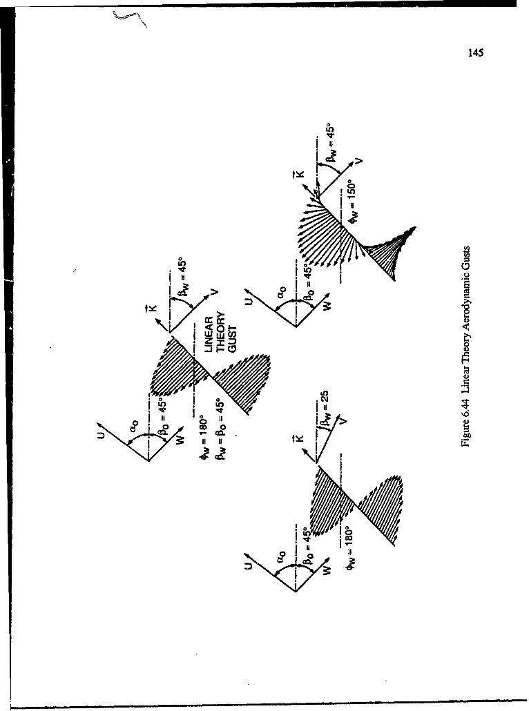
145

0

Iiii

0

U, I Q• .

w UJ 0

z M

.0coi- •i0,)",,i/! ",-

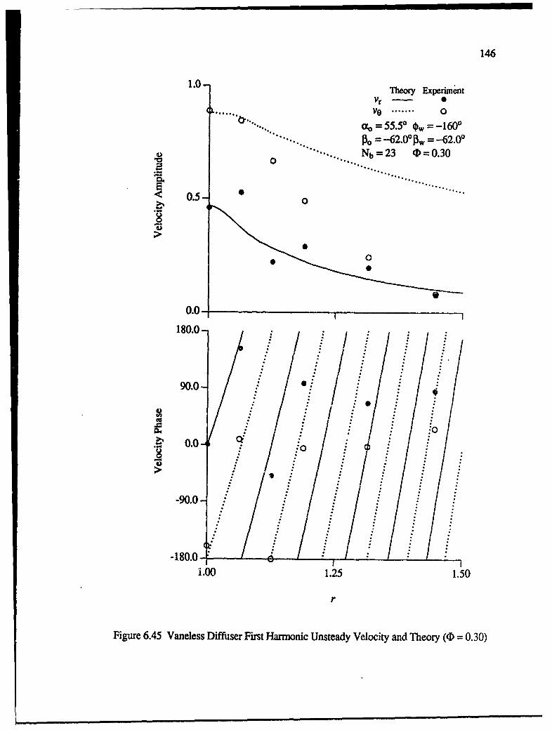
146

1.0-Theory Experiment

Vr - 0Q. ....... Ve ....... 0

"".. = 55.50 O = -1600"Po3 = -62.0°1w = -62.0°

"Nb = 23 (= 0.300

.................... ..........

< 0.5-0

00

0.0

180.0-

90.0-

:0•. 0.0-0

-90.0 1

180.0i.00 1.25 1.50

r

Figure 6.45 Vaneless Diffuser First Harmonic Unsteady Velocity and Theory (0 = 0.30)

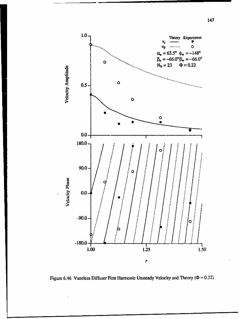
147

1.0- Theory Experimentvr - 0

"o6 = 65.50 * -1480

0 0.= -66.O0P -66.0'~0 N b = 2 3 ( =-0. 2 2

0.5 -. 0....... .. . . .}0 o

180.0-

90.0-:0

S.

.

.

Cu

O •

!

0.0-4

./

-9 0 .0 ---*0:

-180.0- 1

1.00 1.25 1.50

r

Figure 6.46 Vaneless Diffuser First Harmonic Unsteady Velocity and Theory (D = 0.22)

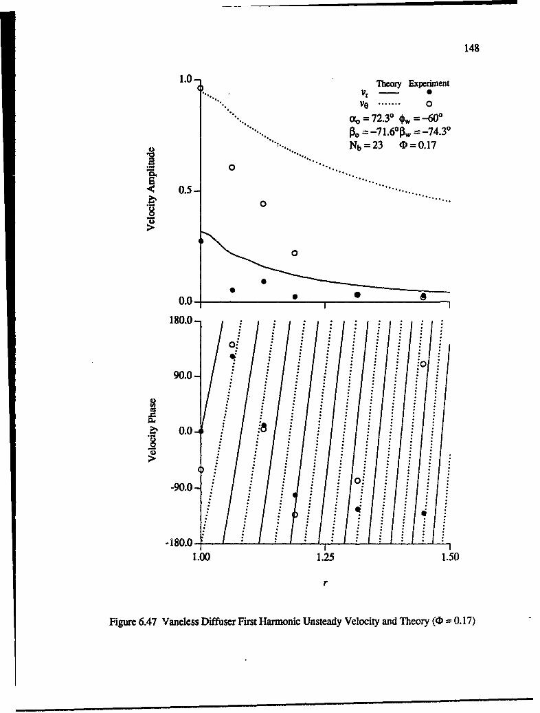
148

1.0 Tleory ExperimentVr 0

(x = 72.30 Ow ='600'""" P = -71.60,w = -74.30

0b .... N 2 3 0 0.17

0.5-

0 ............... . ....... *,

U0 I"180.0-

90.0-

I*0

-90.0-

-180.0-

1.00 1.25 1.50

r

Figure 6.47 Vaneless Diffuser First Harmonic Unsteady Velocity and Theory (0 = 0.17)

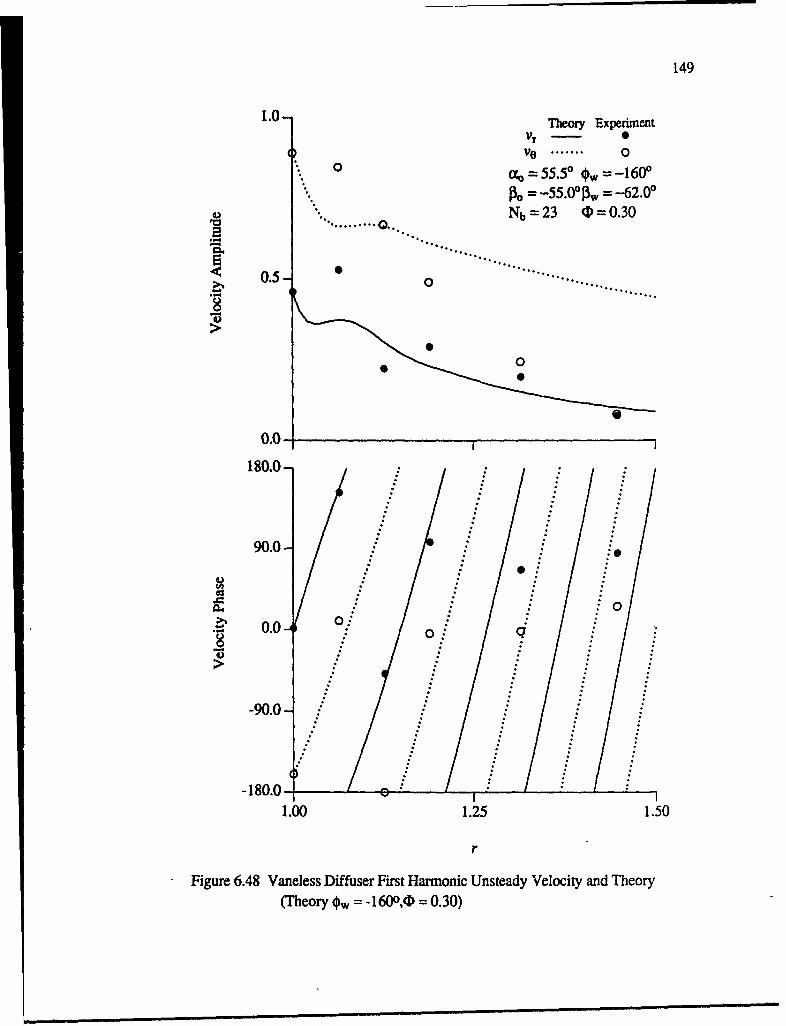
149

1.0- Theory Experiment

Vr - 0

V O ....... 0",, Or, = 55.5* Ow = -160'

" = -55.0o13w -62.0°0. ' . *Nb = 2 3 (= 0.30

..... ..... .....

00

0.0-

180.0-

90.0- :

Ca

I :00.0-4 0

-90.0-

-180.0 -

1.00 1.25 1.50

r

Figure 6.48 Vaneless Diffuser First Harmonic Unsteady Velocity and Theory(Theory Ow = -1600O( = 0.30)

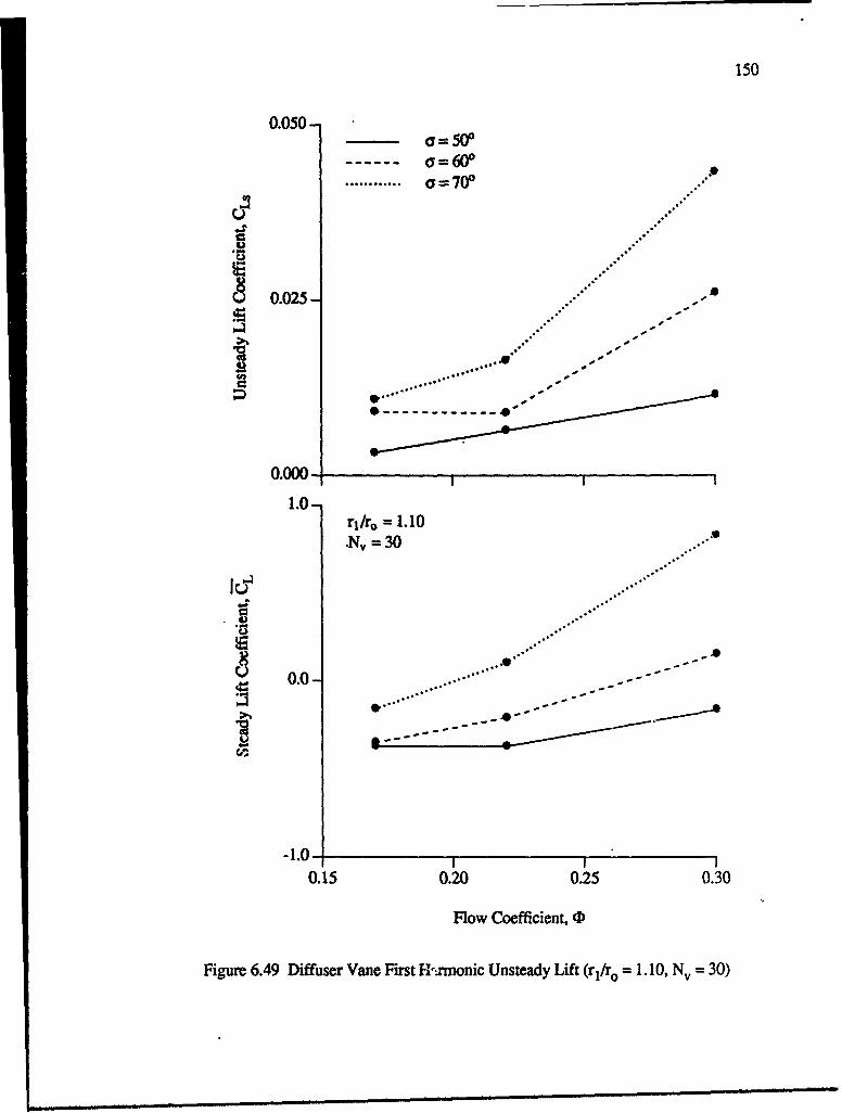
150

0.050-=50

S............ a 70° .

0.025- .

0.000

1.0er/0=1.10

=N,30

0.0-

-1.0-0.15 0.20 0.25 0.30

Flow Coefficient, CID

Figure 6.49 Diffuser Vane First f'.roonic Unsteady Lift (r=/ro 1.10, N0 30)

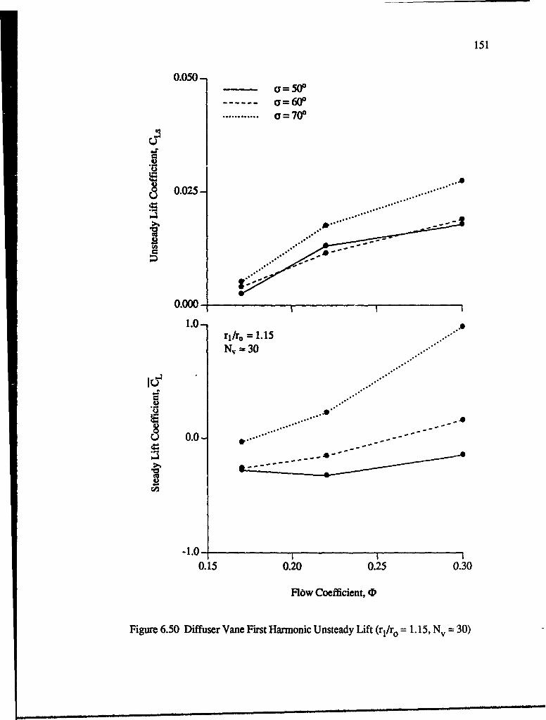
151

0.050- o=50'------ =601

........... =70*

0.025-

0.000,

1.0-rl /ro = 1.15Nv =30

I oo ......U 0.0 .-

-1.00.15 0.20 0.25 0.30

Flow Coefficient, 4'

Figure 6.50 Diffuser Vane First Harmonic Unsteady Lift (rl/ro = 1.15, Nv = 30)

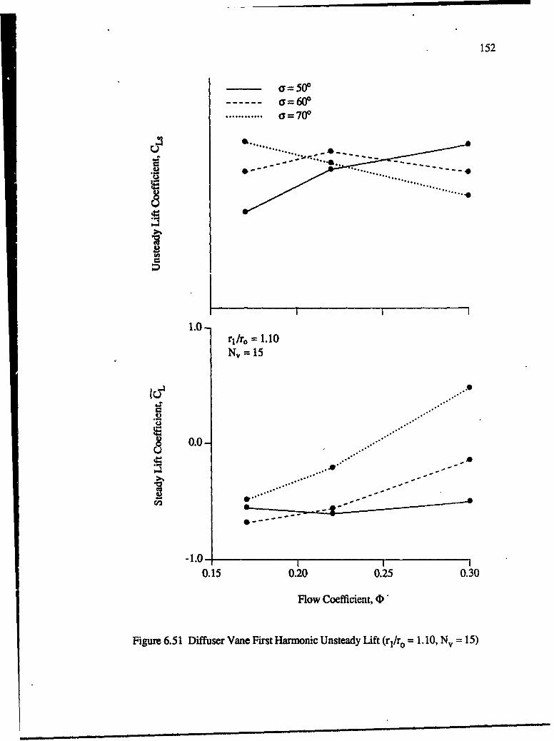
152

a=50'-- a=60o

S............ "=70°

1.0-r1/ro = 1.10N= 15II

8 0.0-U

* ..**

-1.0- .0.15 0.20 0.25 0.30

Flow Coefficient, 0'

Figure 6.51 Diffuser Vane First Harmonic Unsteady Lift (rl/ro = 1.10, Nv = 15)

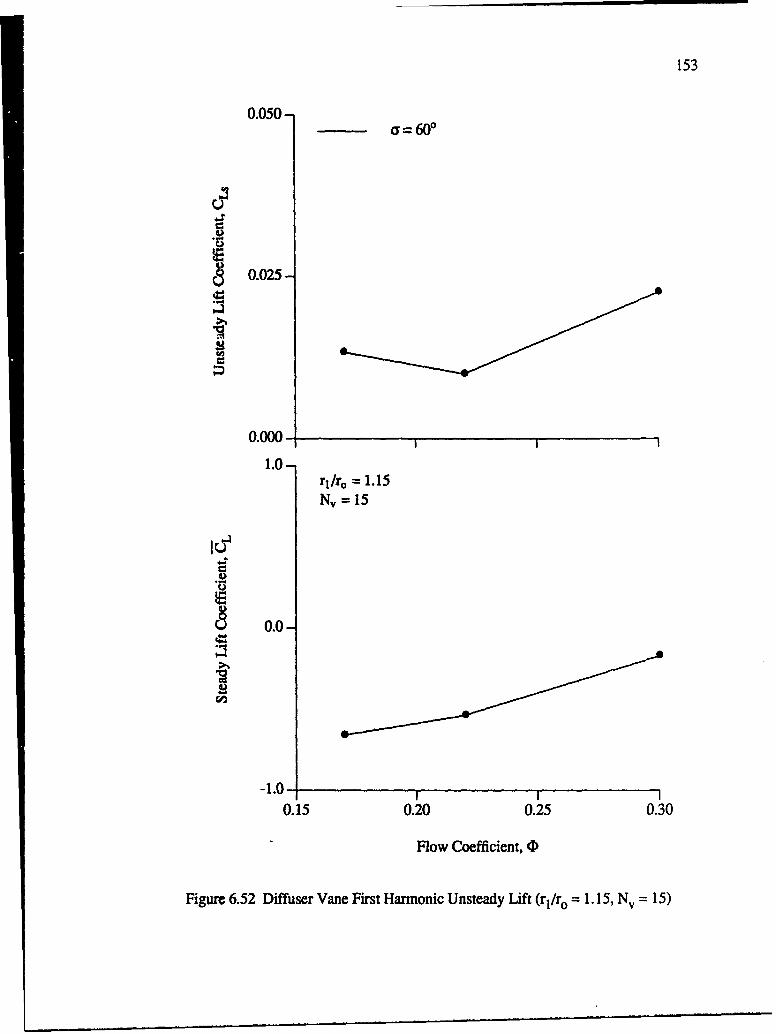
153

0.050-C= 600

S0.025-

0.000 1

1.0-r1/r -- 1.15

N, =15

0.0-

-1.00.15 0.20 0.25 0.30

Flow Coefficient, (D

Figure 6.52 Diffuser Vane First Harmonic Unsteady Lift (rl/ro = 1.15, Nv = 15)

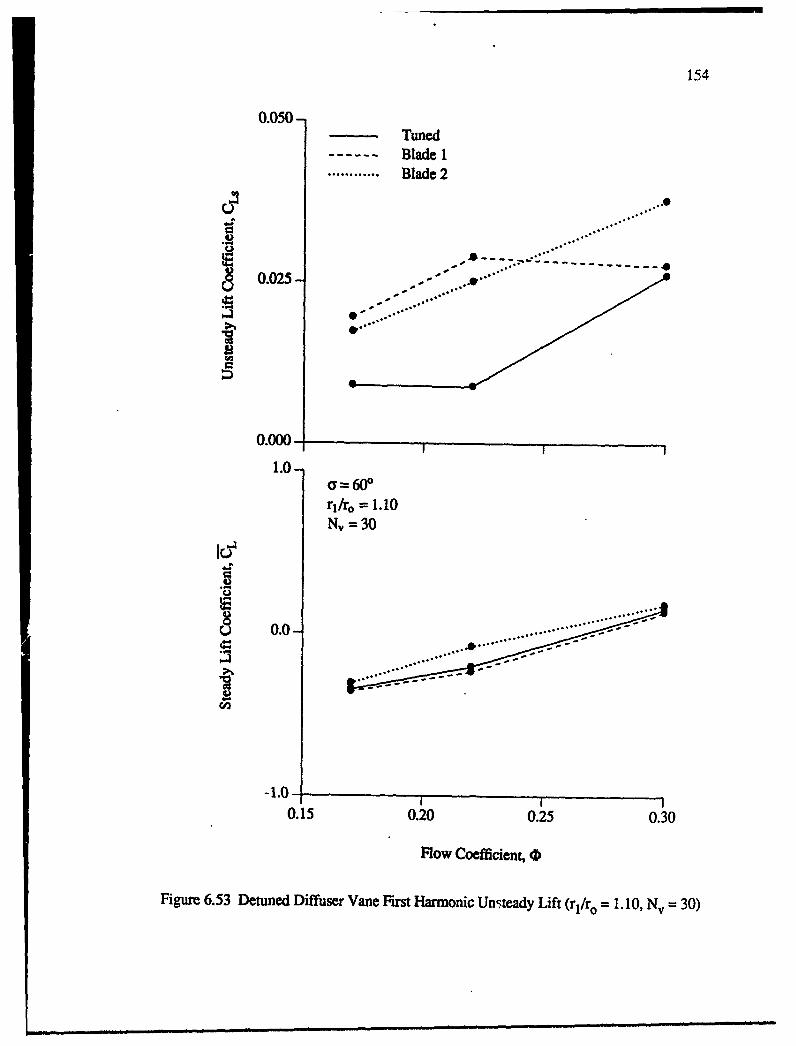
154

0.050 - Tuned

- - Blade I............ Blade2

0.0-2- - - - - - - - -

0.000

1.0-cy 600

rl/r. = 1.10,30

0.0

-1.0I0.15 0.20 0.25 0.30

Flow Coefficient, f

Figure 6.53 Detuned Diffuser Vane First Harmonic Unsteady Lift (rj/ro = 1.10, Nv = 30)

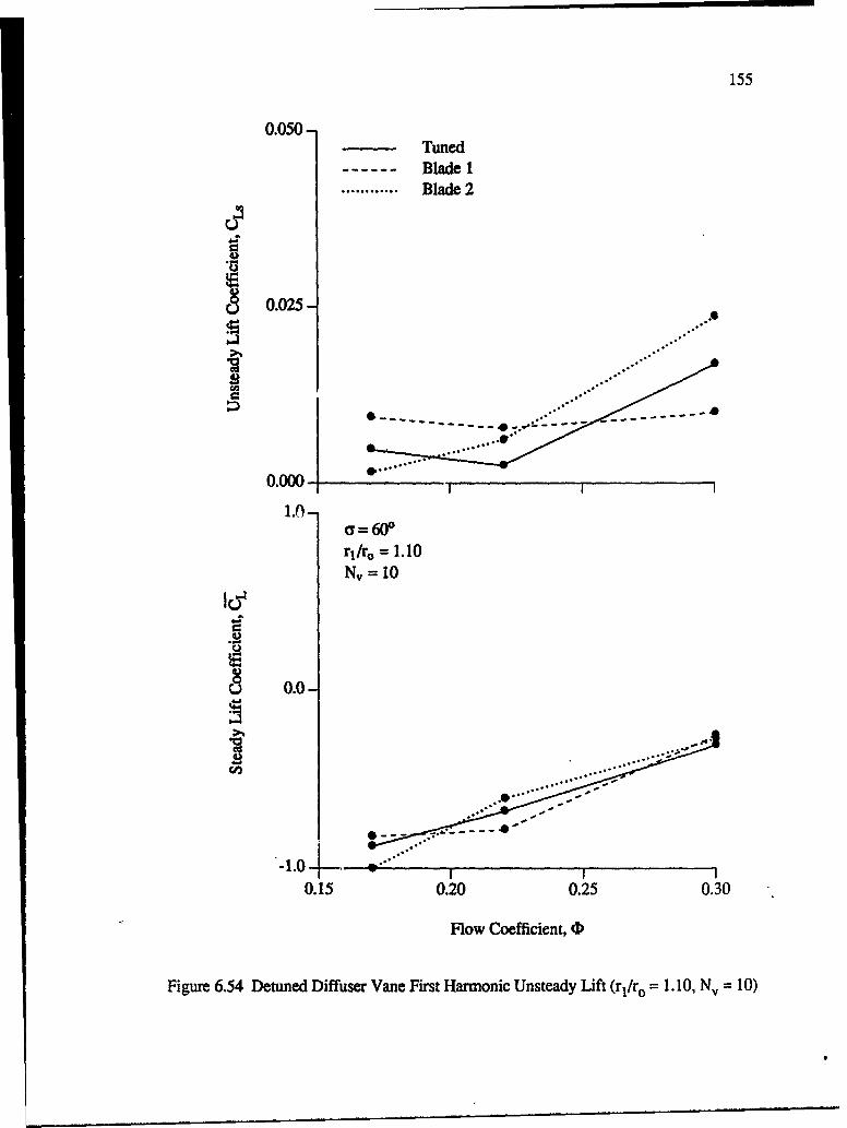
155

0.050-Tuned

- Blade I............ Blade 2

I 0.025-

0.000

1.0=60P

rl/ro = 1.10N, 10

- 0.0-

0.15 0.20 0.25 0.30

Flow Coefficient, (b

Figure 6.54 Detuned Diffuser Vane First Harmonic Unsteady Lift (r1/ro = 1.10, Nv = 10)

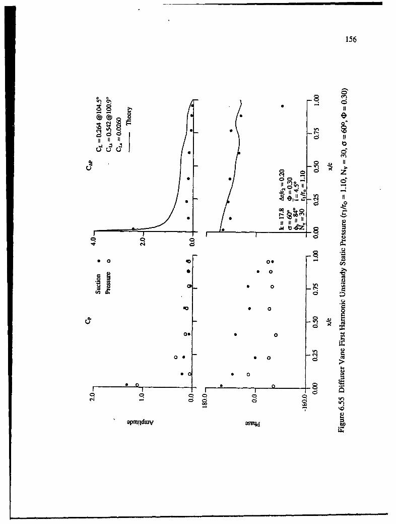
156

00 0

o 0

A 2

C.);

C9 z* ~0 00 -

ItI

0 0

I ~ 0

40 0

00

000 00 4-

0 0 0

0 0 0

0 0

00 k0

4-

OPM*dtu m 0ed

iA

157

0 C0

00) 0 I

0 0-

* 00

6000 0 I

0 0 0

0

ac 0

0 8.

opni~iwV Q-

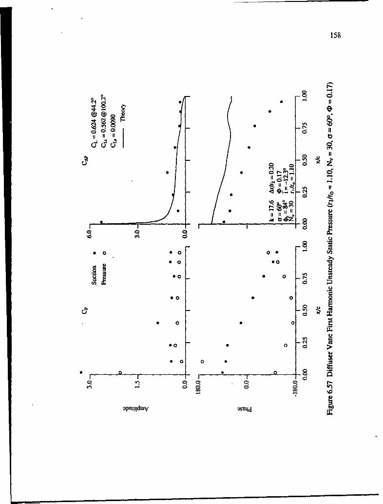
158

* 0~

* III;

00

600 0 r_

0 0 0 0

W)

0. 0

I~(* oo -- •

* 00• 0 .

oo •to -o

00

00 N

* 00

I,,•

opni!IdwV mrqd0T

7 nu., -•~~m mmu 9 HI I I9 mm•

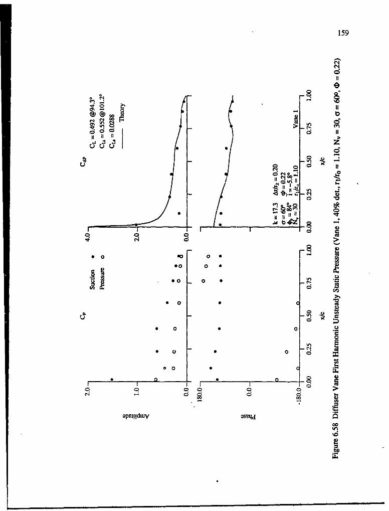
159

Iii

I"

00 0 • _ .

- d d

i • 0 • .

0.0

• oo O I00

0 c"

I I III I ¢

00 00

opmilduttn M'qdt-

o0

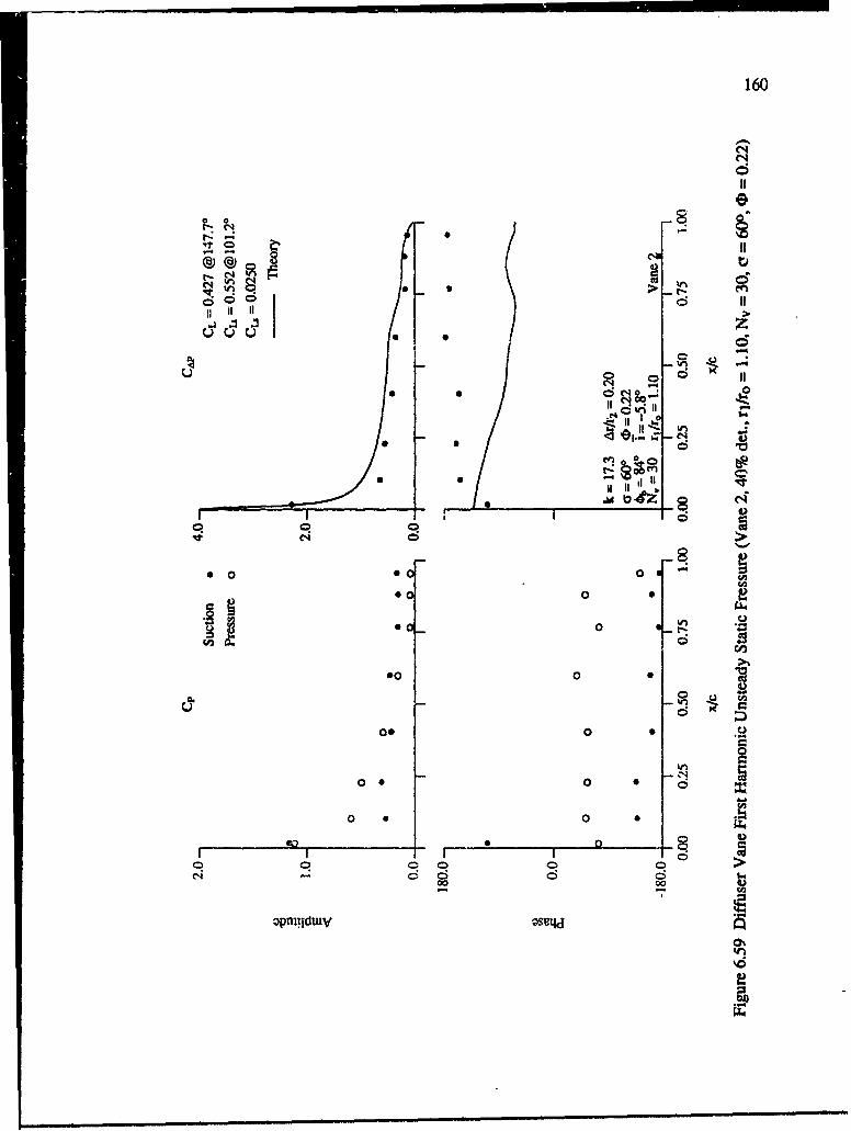
160

lo: -> t-e

CW40 0

ew 042 II

0 0~ 0

C(4

*0 0

000& 0

0 0N

U 0 0 C

00

C!,C40 Cý0 0

00 0 0

0pilw 0 0

* -~ L21

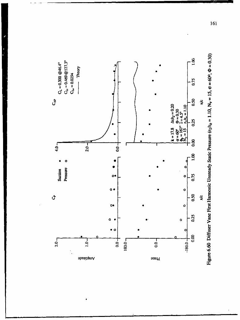
161

0 ',

0 0 C

U 0

00 000

II I)*c

0~ 0 0

00

*~ 0

000

api.dw 0q

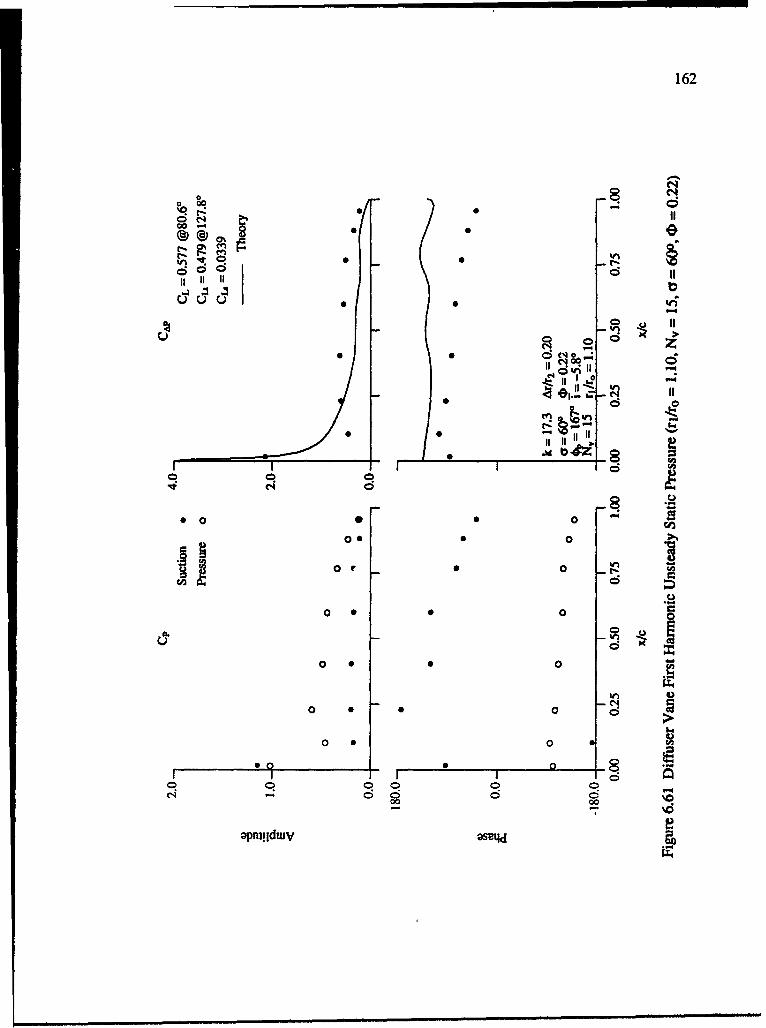
162

Cli

*4 0 I

0 •

0 0

0* 0 0C4

il •."ia

• •° • "q"" I

0 0 0

* .I-•4:Z

0 0 0

0 0 0 as

0 0 0 0

0

0,2

0 0 0

•PnI!ldWV

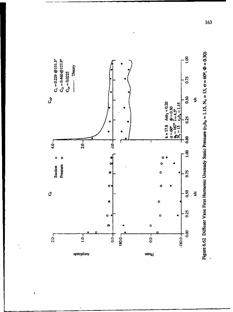
163

000

Of 0 I

0%0

0 0 >

0

* 000

opoidw 0 -l

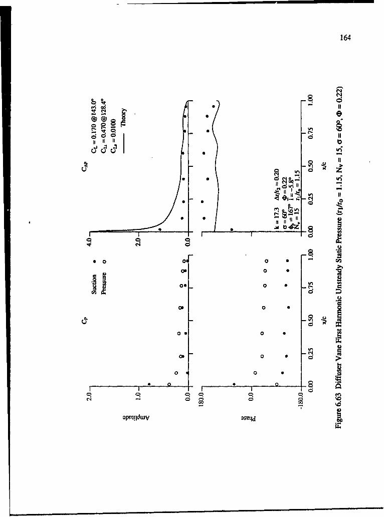
164

en00S•S

Of C.-

II0

0 *5

0 0C i

0 4 0

N II I . o

I IIIIII a

S 00 0 S -•

00

054 00 00

opni!ldwV 'q

i'I, 0 e •

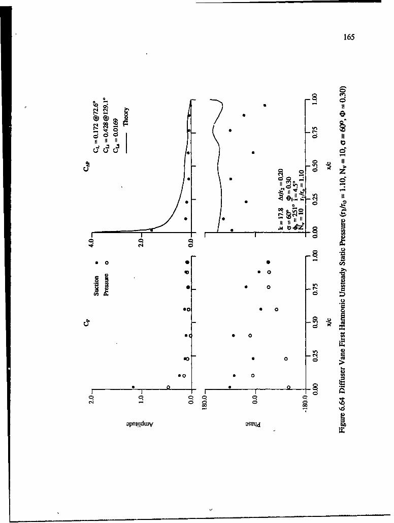
165

000

II'Nl

00 0

I00~i 0~

*c 0 0

C4*0 0 0d

*0 0

00 000

opitdw 0qC.)z

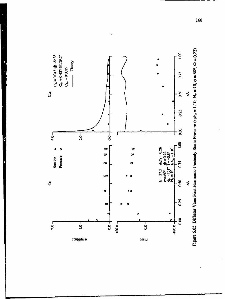
166

00

C4~ 0

00 0 09CI

*b 00 i

00

00 00

ON 0 0

0.0

0 0

40 00

*pliw I-d

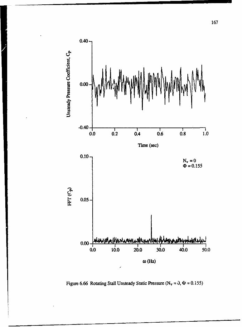
167

0.40-1

-0.40

0.0 0.2 0.4 0.6 0.8 1.0

Timne (sec)

0.10-N,=0

(D = 0. 155

0.05-

0.00-0.0 10.0 20.0 30.0 40.0 50.0

co (Hz)

Figure 6.66 Rotating Stall Unsteady Static Pressure (Nv =0, 0 = 0. 155)

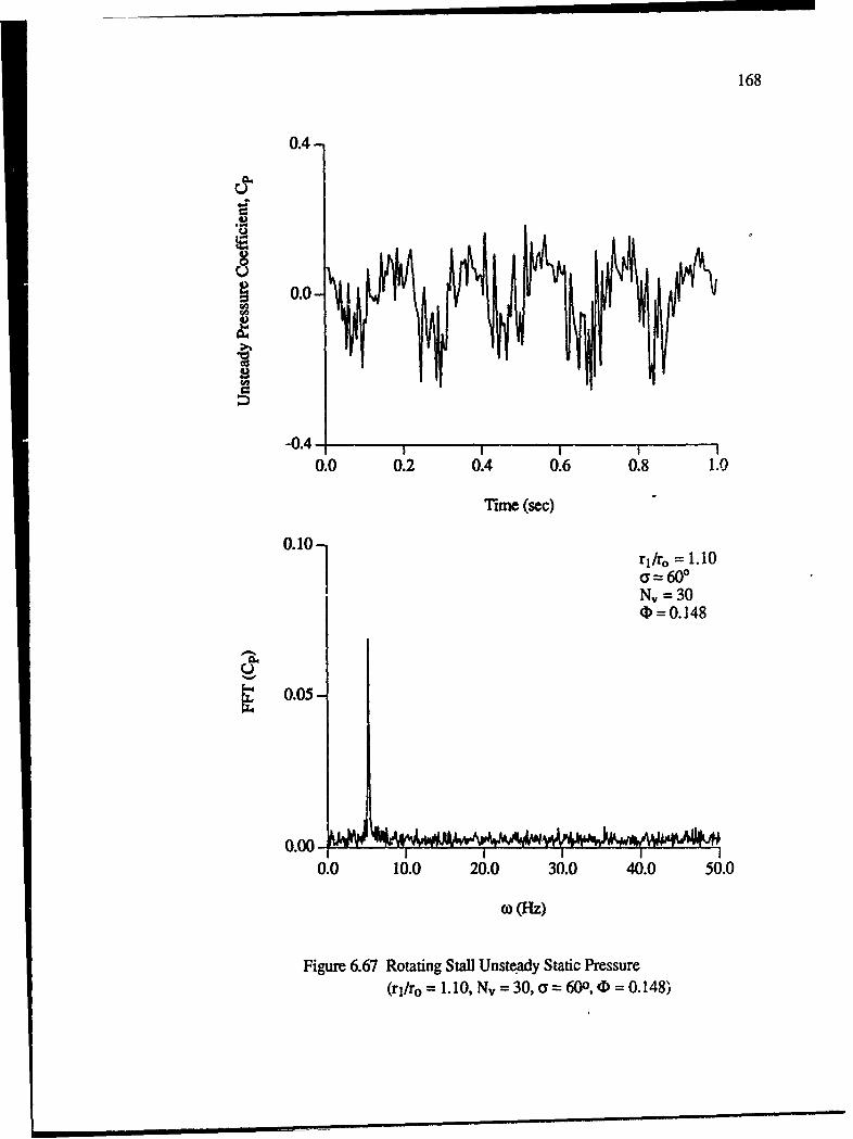
168

0.4-

0.0-

4)

-0.4- 10.0 0.2 0.4 0.6 0.8 1.0

Time (sec)

0.10=~r 1.10

a= 60=Nv = 30(D=0.148

S0.05-

0.0 10.0 20.0 30.0 40.0 50.0

Co (Hz)

Figure 6.67 Rotating Stall Unsteady Static Pressure(rj/ro= 1.10, Nv = 30, a- =60o, ( = 0.148)

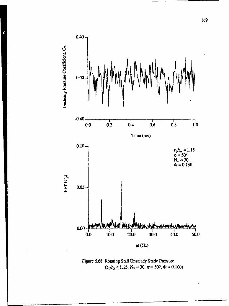
169

0.40o

-0.400.0 0.2 0.4 0.6 0.8 1.0

Tune (sec)

0.10-rl/ro = 1.150=500

N,-30(D =0.160

S0.05-

0.0 10.0 20.0 30.0 40.0 50.0

CO (Hiz)

Figure 6.68 Rotating Stall Unsteady Static Pressure(ri/ro = 1.15, Nv = 30, a= 500, D = 0.160)

170

CHAPTER 7SUMMARY, CONCLUSIONS AND RECOMMENDATIONS

An investigation of some of the unsteady phenomena occurring in centrifugal

compressors has been performed, with the diffuser vane unsteady pressure generated byimpeller wakes of particular interest. It was found that little attention has been devoted in

the literature to the effect of the vaned diffuser on the unsteady aerodynamics inherent in

centrifugal compressors. Therefore, analyses were developed to predict the wake behavior

and diffuser vane unsteady loading. In conjunction with these, a series of experiments was

performed to evaluate this unsteady behavior. The effect of vaned diffuser geometry on thecompressor steady performance and loading as well as surge and rotating stall was

experimentally determined.The performance of the Purdue Research Centrifugal Compressor was measured for

various diffuser geometries. It was found that the vaned diizuser increases efficiency and

overall pressure rise with proper geometry selection. The diffuser stagger angle andnumber of diffuser vanes were seen to be particularly important, with a smaller number of

diffuser vanes generally preferable. The mechanism of this performance improvement wasinvestigated by considering the rotating impeller blade and diffuser vane statc loading. The

vaned diffuser was determined to affect the impeller loading only at higher flow rates withsmall vane loading. The diffuser loading increased with steady incidence and with a

decreasing number of vanes. It was concluded that the vaned diffuser affects the aftimpeller and vaneless space flowfields, reducing mixing and inhibiting secondary flows,

thereby improving performance. Performance improvements were only realized when thediffuser vanes were lightly loaded, with no performance advantage from a loaded diffuser.

The wake velocities in the vaneless radial diffuser were experimentally determined

using laser anemometry. The radial and tangential unsteady wake ,elocities decreasedrapidly with increasing radius, with a greater decrease at lower flow rates. A theoretical

model to predict this behavior was developed by obtaining a solution to the linearized EulerEquations in a radial vaneless diffuser for convected rotational wakes. At higher flow

rates, the theory matched the dam for the radial velocity in a general sense.

171

However, the measured tangential velocity decreased more rapidly with increasing

radius than predicted by the theory. The amplitude ratio and phase angle between the wake

radial and tangential velocities was concluded to affect the correlation with theory, as well

as an unsteady circumferential static pressure generated by the rotating impeller.

Unsteady surface static pressure measurements were made on the diffuser vanes to

determine unsteady loading. The unsteady lift increased with flow rate using 30 diffuservanes, especially at higher vane stagger. Increasing the diffuser leading edge/impeller exit

radial spacing decreased the lift at higher flow rates and stagger angles, although at lower

flow rates, the effect was less pronounced. With 15 diffufer vanes, the unsteady lift was

generally greater, with less variation due to flow rate. Increasing the diffuser leading

edge/impeller exit radial spacing decre'•sed the unsteady lift significantly. Nonuniform

circumferential spacing detuning increased the lift on one or both of the vanes in all cases.

A theory to predict the unsteady diffuser vane loading was developed by applying

conformal mapping to existing axial cascade unsteady aerodynamic theory and

incorporating the wake model as a boundary condition. Poor correlation of the data with

the theory was seen with 30 diffuser vanes, which was attributed to the very close vane

spacing. Reasonable correlation between data and theory was seen with 15 diffuser vanes

at points of low vane steady loading. An unexplainable poor correlation with theory was

seen using 10 diffuser vanes. Mismatch of data with theory is believed to be due tomismatch of the wake model and steady loading on the diffuser vanes, which the theory

does not consider.

Finally, flow instabilities in the compressor were experimentally investigated. A one-lobed impeller stall existed at low flow coefficient for the vaneless diffuser. For the vaned

diffuser, several instabilities were observed. With 30 diffuser vanes, diffuser stall andsurge were the only instabilities occurring. For 600 vane stagger, surge typically occurred

at a flow coefficient of approximately 0.155, with rotating stall not observed. At the higher

diffuser vane leading edge/impeller exit ratio for 600 vane stagger, the compressor wasoperated at very low flow coefficient without surge or rotating stall. With 15 diffuser

vanes, the impeller stalled before the diffuser, with surge again occurring at 600 vane

stagger without rotating stall occurence.. It was seen that localized vane stalling was not a

sufficient condition for rotating stall to occur. Also, significant improvement in stall

margin was realized by proper adjustment of the vaned diffuser.

The recommendations for further study are basically twofold. First, further

experimental investigation is needed to more accurately determine the parameters that affect

the impeller/radial diffuser unsteady wake behavior. The determination of how the

172

amplir:de ratio and phase angle between the wake velocities affect the wake behavior andhow these vary with impeller geometry, operating point and ro. "tonal speed would beuseful. More data on unsteady diffuser vane loading would also be beneficial to moreaccurately determine the effects of diffuser vane row geometry on the unsteady response.More evidence on the effect of diffuser geometry on rotating stall would also be asignificant experimental contribution. Since the current investigation was performed at lowspeed, it is important to establish the correlation between measurements made at low speedand behavior of high speed machines.

The second recommendation concerns the theoretical prediction of unsteady behavior.A more accurate model for radial diffuser wake behavior would certainly be useful. It islikely a model that considers the circumferential pressure variation as a boundary conditionwill be necessary. Once this is accomplished, incorporating this model into unsteady vaneloading prediction is of primary importance. The effects of vane loading and gustdistortion should be considered in the unsteady loading analysis. Since the unsteadydii'fuser vane loading analysis is only valid for incompressible flow, prediction of unsteadyloading in high speed machines will require consideration of compressibility effects.

In conclusion, a more significant data base along with more general analyses will benecessary before accurate prediction of unsteady aerodynamics in centrifugal compressors

is realized.

LIST OF REFERENCES

173

LIST OF REFERENCES

Arndt, N.; Acosta, A.J.; Brennen, C.E. and Caughey, T.K. "Rotor-Stator Interaction in aDiffuser Pump," ASME Paper 88-GT-55, 1988.

Bammert, K.; Jansen, M. and Rautenberg, M. "On the Influence of the Diffuser InletShape on the Performance of a Centrifugal Compressor Stage," ASME Paper 83-GT-9, 1983.

Bryan, W. B. and Fleeter, S. "The Effect of Prewhirl on the Internal Aerodynamics andPerformance of a Mixed Flow Research Centrifugal Compressor," Thermal Sciencesand Propulsion Center Technical Report, ME-TSPC-TR-87-12, Purdue University,August 1987.

Bryan, W.B. and Fleeter, S. "Flow Induced Forced Response of an IncompressibleRadial Cascade Including Profile and Incidence Effects," AIAA Paper 90-2352, July,1990.

Bryer, D. W. and Pankhurst, R. C. Pressure Probe Methods for Determining Wind Speedand Flow Directon, London: Her Majesty's Stationery Office, 1971.

Capece, V. R. and Fleeter, S. "Forced Response Unsteady Aerodynamics in a MultistageCompressor," Thermal Sciences and Propulsion Center Report, ME-TSPC-TR-87-12, Purdue University, August, 1987.

Caruthers, J. E. and Kurosaka, M. "Flow Induced Vibration of Diffuser Excited RadialCompressors," Final Report NAG 3-86, Septermber 1982.

Cebeci, T. and Bradshaw, P. Momentum Transfer in Boundary Layers, McGraw Hill,New York, 1977.

Chiang, H. W. D. "Aerodynamic Detuning of a Loaded Airfoil in an Incompressible Flowby a Locally Analytical Method," PhD Thesis, Purdue University, August 1988.

Churchill, R.V. and Brown, J.W. Complex Variables and Applications, McGraw Hill,New York, 1984.

Clements, W. W. and Artt, D. W. "The Influence of Diffuser Channel Geometry or. theFlow Range and Efficiency of a Centrifugal Compressor," Proceedings of theInstitutionn of Mechanical Engineers, Vol 201, No. A2, 1986, pp. 145 -152.

174

Dean, R. C. "On the Necessity of Unsteady Flow in Fluid Machines," ASME Journal ofBasic Engineering, Vol. 87, March, 1959, pp. 24-28.

Dean, R. C. and Senoo, Y. "Rotating Wakes in Vaneless Diffusers," ASME Journal ofBasic Engineering, Vol. 88, January 1960, pp. 49-60.

Dixon, S. L. Thermodynamics of Turbomac;dnery, Pergamon Press, Oxford, 1978.

Eckardt, D. "Instantaneous Measurements in the Jet-Wake Discharge Flow of a CentrifugalCompressor Impeller," ASME Journal of Engineering for Power, July 1975, pp.337-345.

Emmons, H. W.; Pearson, C. F. and Grant, H. P. "Compressor Surge and StallPropagation," Transactions of the ASME, Vol. 79, 1955.

Fagan, J. R. "An Investigation of the Three-Dimensional Flow Field in a CentrifugalCompressor," Ph.D. Thesis, Purdue University, June, 1989.

Faulders, C.R. "Aerodynamic Design of Vaned Diffusers for Centrifugal Compressors,"ASME Technical Paper 56-A-213, 1956.

Fisher, E. H. and Inoue, M. "A Study or Diffuser/Rotor Interacton in a CentrifugalCompressor," Journal of Mechanical Engineering Science, Vol. 23, No. 3, 1981.

Goldstein, M. E. and Atassi, H. "A Complete Second-Order Theory for the UnsteadyFlow about an Airfoil due to a Periodic Gus,,' Journal of Fluid Mechanics, Vol. 74,Part 4, 1976, pp 741-765.

Gostelow, J. P. Cascade Aerodynamics, Pergamon Press, Oxford, 1984.

Grietzer, E. M. "The Stability of Pumping Systems-The 1980 Freeman Scholar Lecture,"ASME Journal of Fluids Engineering, Vol. 103, pp 193-242, June 1981.

Henderson, G. "Forcing Function and Steady Loading Effects on Unsteady AerodynamicGust Response," PhD Thesis, Purdue University, August 1991.

Hoyniak, D. and Fleeter, S. "Prediction of Aerodynamically Induced Vibrations inTurbomachinery Blading," ASME Journal of Fluids Engineering, Vol. 105, pp 375-381, December 1983.

Inoue, M. and Cumpsty, N.A. "Experimental Study of Centrifugal Impeller DischargeFlow in Vaneless and Vaned Diffusers," ASME Journal of Engineering for GasTurbines and Power, April, 1984, Vol. 106, pp. 455 -467.

175

Krain, R- "Swirling Impeller Flow," ASME Paper 87-GT-19, June 1987.

Panton, R. L. Incompressible Flow, Wiley-Interscience, New York, 1984.

Rodgers, C. "The Performane of Ce~atrifugal Compressor Channel Diffusers," ASMEPaper 82-GT-10, 1982.

Ross, S.H. Introducion to Ordinary Differential Equations, John W~iey and Sons, 1980.

Scheaffer, Richard L. and McClave, James T. Statistics for Engineers, Duxbury Press,Boston, 1982..

Senoo, Y. and Ishida, M. "Behavior of Severely Asymmetric Flow in a VanelessDiffuser," ASME Journal of Engineering for Power, Vol. 97, 1975, pp. 375-387.

Smith, V. J. "A Review of the Design Practice and Technology of Radial CompressorDiffusers," ASME Technical Paper 70-GT- 116, 1970.

Van den Braembussche, R. "Surge and Stall in Centrifugal Compressors," von KarmanInstitute for Fluid Dynamics Lecture Series 1984-07, May 28-30, 1984.

Vavra, M. H. and Gawain, T. H. "Compressor Test Rig For Investigation of FlowPhenomena in Turbo-Machines," Technical Report No. 12 on Project No. NP. 061-058, February, 1955.

Verdon, Joseph M. "The Unsteady Flow in the Far Field of an Isolated Blade Row,"United Technologies Research Center Report R87-957333-1, April, 1987.

Whitehead, D.S., "Force and Moment Coefficients for Vibrpting Aerofoils in Cascade,"Aeronautical Research Council Reports and Memoranda No. 3254, February, 1960.

Whitehead, D.S. "Classical Two-Dimensional Methods," AGARDograph No. 298,AGARD Manual on Aeroelasticity in Axial Flow Turbomachines, Volume 1:Unsteady Turbomachinery Aerodynamics, 1984, pp. 3.1-3.30.

Wood, J.R.; Adam, P.W. and Buggele, A.E. "NASA Low-Speed CentrifugalCompressor For Fundamental Research," NASA Technical Memorandum 83398,1983.

Yoshinaga, Y.; Gyobu, I.; Mishina, IH.; Koseki, F. and Nishida, H. "AerodynamicPerformance of a Centrifugal Compressor with Vaned Diffusers," ASME Journal ofFluids Engineering, Vol. 102, December 1980.

176

Zachmanoglou, R.C. and Thoe, D.W. Introduction to Partial Differential Equations withApplications, Dover Publications, Inc., New York, 1986.