AN INVESTIGATION OF TRENDS IN CARBONACEOUS AEROSOLS OVER

NORTH AMERICA

by

Sara Torbatian

Submitted in partial fulfilment of the requirements

for the degree of Master of Science

at

Dalhousie University

Halifax, Nova Scotia

August 2013

© Copyright by Sara Torbatian, 2013

ii

To my parents, Maryam & Mehdi

and my lovely sister, Zahra

iii

TABLE OF CONTENTS

LIST OF TABLES ............................................................................................................. iv

LIST OF FIGURES ............................................................................................................ v

ABSTRACT ..................................................................................................................... viii

LIST OF ABBREVIATIONS USED ................................................................................ ix

ACKNOWLEDGEMENTS ............................................................................................... xi

CHAPTER 1 INTRODUCTION ........................................................................................ 1

1.1 Motivation …………………………………………………………………….1

1.2 Aerosols……………………………………………………………………….2

1.3 Carbonaceous Aerosol………………………………………………………...3

1.4 Historical Trend……………………………………………………………….5

CHAPTER 2 Analysis of Emission Inventories of Carbonaceous Aerosol…………….16

2.1 Trend Analysis………………………………………………………………16

2.2 Bottom-up emission inventories of BC and OC...……….………………….22

2.3 Inventory Evaluation…………………………………………..………….…41

2.4 "Top-down" Estimate of Anthropogenic Sources …………………………..45

CHAPTER 3 CONCLUSION ......................................................................................... 50

3.1 Summary……………………………………………………………………...50

3.2 Future Directions………………………………………………………….…51

BIBLIOGRAPHY ............................................................................................................. 52

APPENDIX A The time series of wood consumption ................................................... 56

iv

LIST OF TABLES

Table 1.1 Standard equations used by IMPROVE to convert the measured fine

aerosol mass to aerosol species concentrations (Malm et al., 2004)….....

8

Table 2.1 Total values of BC and OC emission (Tg/yr) estimated by three

emission inventories (Bond, RCP, and MACCity) and averaged over

North America, West, and East of North America for years 1980, 1990,

and 2000…………………………………………………………………

26

Table 2.2 Total emission values of black carbon (Tg/yr) for years 1990, 2000, and

2010 derived from the new database……………………………………

34

Table 2.3 Total emission values of organic carbon (Tg/yr) for years 1990, 2000,

and 2010 derived from the new database……………………………..…

38

Table 2.4 The scale factors computed based on multiple linear regression for

different sectors (residential west, residential east, industry, power, and

transport)…………………………………………………………………

47

v

LIST OF FIGURES

Figure 1.1 Climate forcing of different factors (source ww.ipcc.ch)......................... 5

Figure 1.2 Map of IMPROVE sites December 2010 (IMPROVE, 2011, Ch1)……. 6

Figure 1.3 Schematic view of the IMPROVE sampler with four modules

(IMPROVE, 2011, Ch1)………………………………………………...

7

Figure 1.4 Seasonal variability of IMPROVE 2005-2008 monthly mean POM (a)

and LAC (b) concentrations. The upward triangle corresponds to the

season with maximum concentration and the downward triangle is

corresponded to the season with the minimum concentration. The

seasons are identified by different colors. The size of the triangles is

determined by the ratio of maximum to minimum mean concentration...

11

Figure 1.5 Long-term (1989-2008) trends of total carbon mass concentrations for

winter (% yr-1

) (IMPROVE, 2011, Ch6)………………………………...

12

Figure 1.6 Long-term (1989-2008) trends of total carbon mass concentrations for

summer (% yr-1

) (IMPROVE, 2011, Ch6)………………………………

13

Figure 1.7 Short-term (2000-2008) trends of total carbon mass concentrations for

winter (% yr-1

) (IMPROVE, 2011, Ch6)………………………………...

14

Figure 1.8 Short-term (2000-2008) trends of total carbon mass concentrations for

summer (% yr-1

) (IMPROVE, 2011, Ch6)………………………………

14

Figure 2.1 Long-term (1989-2008) trends (%yr-1

) of black carbon, organic carbon,

and total carbon concentrations (TC = organic carbon + black carbon)

in winter months measured by the IMPROVE network………………...

18

Figure 2.2 Concentration of black carbon (left) and organic carbon (right) (µg m-

3). The in situ observations shown by circles are three year averages

for 1989-1991, 1999-2001, and 2008-2010. The background contours

represent the outputs of GEOS-Chem simulations for 1990, 2000, and

2010 emissions (Leibensperger et al., 2012).............................................

20

Figure 2.3 A comparison of the trend of simulation outputs with observations

calculated using Theil regression for 1990-2010 for annual data (a) and

for winter months (b)………………………………………………........

21

Figure 2.4 A comparison of the winter (DJF) time series of the observed

(IMPRVE measurements) and GEOS-Chem model output from

Leibensperger et al. (2012) averaged over sites in the west, far west,

vi

east and the whole US for black carbon and organic carbon (µg m-

3)…………………………………………………………………………

23

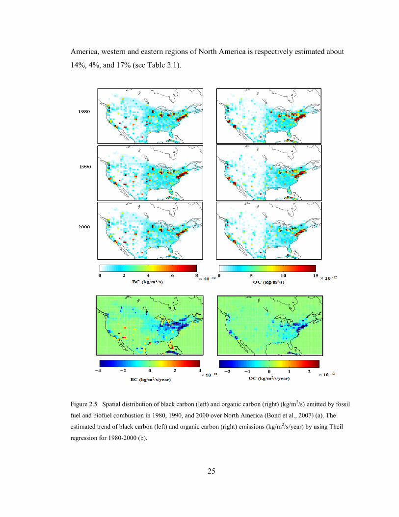
Figure 2.5 Spatial distribution of black carbon (left) and organic carbon (right)

(kg/m2/s) emitted by fossil fuel and biofuel combustion in 1980, 1990,

and 2000 over North America (Bond et al., 2007) (a). The estimated

trend of black carbon (left) and organic carbon (right) emissions

(kg/m2/s/year) by using Theil regression for 1980-2000 (b)…………….

25

Figure 2.6 The Map of black carbon (left) and organic carbon (right) emissions

from fossil fuel and biofuel combustions derived from Lamarque

inventory in 1980, 1990, and 2000 (kg/m2/s) over North America

(Lamarque et al., 2010) (a). The calculated trend of black carbon (left)

and organic carbon (right) emissions (kg/m2/s/year) based on the Theil

regression method for 1980-2000 (b)……………………………………

28

Figure 2.7 The seasonal trend of black carbon (top) and organic carbon (bottom)

emissions (kg/m2/s/year) of MACCity inventory estimated by using

Theil regression for 1990-2010 (Lamarque et al., 2010)………………..

29

Figure 2.8 The comparison of the trends of BC and OC annual emissions

(kg/m2/s/year) (left) with the trends of surface concentrations of BC

and OC (µg/m3/year) for winter (right). The trends are computed by

applying the Theil regression method for 1990-2000…………………...

29

Figure 2.9 A comparison of the trend of annual emissions (left) with the trend of

surface concentrations of BC and OC (%year-1

) for winter (right) for

1990-2000…………………………………………………….

30

Figure

2.10

The time series of North American emissions (the new database, and

the ANL database) (kg/year) for 1995-2010 for BC and OC……………

33

Figure

2.11

Seasonal and spatial distribution of black carbon (top) and organic

carbon (bottom) emissions (kg/m2/s) for the year 2006 over North

America derived from the new database………………………….……..

34

Figure

2.12

Spatial distribution of black carbon emission for years 1990, 2000, and

2010 for four different sectors (residential, industry, power, and

transport) (kg/m2/s) derived from the new database throughout North

America………………………………………………………………….

35

Figure

2.13

The trend of black carbon emission for different sectors (residential,

industry, power, and transport) (kg/m2/s/year) estimated by the new

database for 1990-2010………………………………………………….

36

Figure Spatial distribution of the fraction of each sector of black carbon

vii

2.14 emission for years 1990, 2000, and 2010 (%) derived from the new

database. The values written in the figure are the total black carbon

absolute emission for each year…………………………………………

37

Figure

2.15

Spatial distribution of organic carbon emission for years 1990, 2000,

and 2010 for four different sectors (residential, industry, power, and

transport) (kg/m2/s) estimated by the new database throughout North

America………………………………………………………………….

38

Figure

2.16

The trend of organic carbon emitted from different sectors (residential,

industry, power, and transport) (kg/m2/s/year) derived from the new

database for 1990-2010………………………………………………….

39

Figure

2.17

Spatial distribution of the fraction of each sector of organic carbon

emission for years 1990, 2000, and 2010 (%) derived from the new

database. The total organic carbon absolute emission values are written

for each year……………………………………………………………..

40

Figure

2.18

A Comparison of simulation outputs with the observations of BC and

OC surface concentrations (µg/m3

) in winter. Observations are three-

year averages for 1988-1990, 1994-1996, 1999-2001, 2004-2006, and

2008-2010 measured by IMPROVE. GEOS-Chem model outputs are

derived from winter time simulation for 1989, 1995, 2000, 2005, and

2010……………………………………………………………………...

43

Figure

2.19

The difference between the simulation outputs and observations for

black carbon (top panel) and organic carbon (bottom panel) for winter

season of the years 1989, 1995, 2000, 2005, and 2010………………….

44

Figure

2.20

A comparison between the observed and simulated trend of BC and OC

concentrations by using Thiel regression. The simulated trend is

calculated for winter season of the years 1989, 1995, 2000, 2005, and

2010. The observed trend is computed for winter season of 1989-2010

(µg m-3

year-1

)……………………………………………………………

44

Figure

2.21

A comparison of the observed trend with the simulated trend derived

from (a) initial guess of emission scale factor (b) the optimized scale

factors (µg m-3

year-1

) for BC and OC during winter time of 1989-2010.

The third column shows the difference of the observed and simulated

trend. The root mean-square deviation is calculated for each case……..

48

Figure

2.22

A comparison between the observed trend in BC and OC

concentrations (%year-1

) with the resulting simulated trend for winter

1989-2010. ……………………………………………………………...

49

viii

ABSTRACT

A long term (1989-2008) decreasing trend in black carbon and organic carbon surface

concentrations is indicated by insitu measurements (IMPROVE) in the United States in

winter months. The observed percent negative trend is higher in the western United States

than the eastern region. This study examines how the observed trend relates to emission

inventories of black carbon and organic carbon. Attention is paid to the contribution of

emissions from the residential sector to the observed decreasing trend particularly over

the western United States. A chemical transport model is used to relate the emission

inventories to concentrations. A variety of bottom-up emission inventories are tested.

Multiple linear regression was used to estimate the anthropogenic sources contributing to

trends in BC and OC concentrations in winter months over US. The larger relative trend

of carbonaceous aerosols in the west appears to be driven by the larger relative

contribution of residential and transport sources to this region.

ix

LIST OF ABBREVIATIONS USED

AeroCom Aerosol Comparisons between observations and models

AL Aluminium

ANL Argonne National Laboratory

ARCTAS Arctic Research of the Composition of the Troposphere from

Aircraft and Satellites

BC Black Carbon

Ca Calcium

CAC Criteria Air Contaminants

CCN Cloud Condensation Nuclei

CM Coarse Mass

CO3 Carbonate

CTM Chemical Transport Model

EC Elemental Carbon

EPA Environmental Protection Agency

Fe Iron

FM Fine Mass

FeO Iron (II) oxide

Fe2O3 Iron (III) oxide

GEOS Global Earth Observing System

GFED Global Fire Data

H2O Water

IMPROVE Interagency Monitoring of Protected Visual Environments

IPCC Intergovernmental Panel on Climate Change

LAC Light Absorbing Carbon

MACCity Monitoring Atmospheric Composition & Climate

MgO Magnesium oxide

NASA National Aeronautics and Space Administration

Na2O Sodium oxide

NCAP National Carbonaceous Aerosols programme

x

NEI National Emission Inventory

NO3 Nitrate

NOx Nitrogen oxide

OC Organic Carbon

OMC Organic Carbon Mass Concentration

POA Primary Organic Aerosol

POM Particulate Organic Matter

PM2.5 particulate matter with diameters less than 2.5 µm

PM10 particulate matter with diameters less than 10 µm

RCP Representative Concentration Pathways

RETRO Reanalysis of the tropospheric chemical composition

S Sulfate

Si Silicon

SOA Secondary Organic Aerosol

SO2 sulphur dioxide

TC Total Carbon

Ti Titanium

TOR Thermal Optical Reflectance

UNEP United Nations Environment Programme

xi

ACKNOWLEDGEMENTS

I would like to thank sincerely from my supervisor, Dr. Randall Martin for

his constructive supervision and enormous support during my study.

I am very grateful to my supervisory committee, Dr.Jeff Pierce for his

positive guidance. I would like to thank individuals of my office mates at

Atmospheric Composition Analysis Group specially Sajeev Philip, Aaron

van Donkelaar, Brian Boys, Colin Lee and Akhila Padmanabhan for their

collaboration and assistance. I would like to thank the staff and colleagues

at Department of physics and Atmospheric Science for their kind support

during my Master’s study.

Finally, I would especially like to thank my parents and my sister, Zahra for

their endless emotional support and constant encouragement in these years.

1

CHAPTER 1 INTRODUCTION

1.1 Motivation

Atmospheric aerosols have significant effects on air quality and Earth’s climate.

Numerous studies have found a strong relationship between fine particle concentration

and severe health effects such as enhanced mortality, cardiovascular, respiratory, and

allergic diseases (Querol et al., 2001, and Dockery et al., 1993). Particulate matter

(particles with diameter 2.5 μm or less) can penetrate deep into the lungs and cause

serious respiratory problems. These small particles can enter the bloodstream and can

cause further problems. The physical and chemical properties of aerosols such as their

size, mass concentration, solubility, and chemical composition determine their negative

health effects (Poschl et al., 2005).

Aerosols can affect Earth’s radiation balance directly by scattering or absorbing solar

radiation (short wave) and terrestrial radiation (thermal) which can cause either cooling

(negative radiative forcing) or warming (positive radiative forcing) of the atmosphere.

Visibility impairment or haze is a related process which can be readily observed.

According to a report of the Intergovernmental Panel on Climate Change (IPCC), the

direct climate forcing of aerosol causes a global mean negative radiative forcing of -0.5 ±

0.4 W/m2, while greenhouse gases have a positive radiative forcing of +2.6 ± 0.3 W/m

2

(Forster et al., 2007). The size and spatial distribution, and chemical composition of

aerosols determine their net effect on the global climate system (Poschl et al., 2005). In

addition, aerosols are able to modify the radiation balance indirectly. They play a vital

role in cloud formation, acting as seeds for cloud droplet formation (Cloud Condensation

Nuclei, CCN). The increase in aerosol concentration raises the number of cloud droplets

which leads to reflecting more sunlight into the space (first indirect effect). In addition,

the increase in CCN can reduce the size of cloud droplets. Since smaller droplets need

more time to coalesce into large enough droplets for falling, the cloud lifetime would

increase (second indirect effect) (Albrecht, 1989). Overall, aerosols have a cooling effect

2

on Earth’s climate considering their direct and indirect effects, but there are a lot of

uncertainties in this regard (IPCC, 2007).

Although aerosols represent a small fraction of atmospheric mass, they have a

disproportionately large impact on global climate, visibility and public health. The

importance of understanding aerosols is therefore stressed.

1.2 Aerosols

Aerosols are tiny particles in solid or liquid form suspended in the atmosphere with a

wide range of size, concentration and chemical composition which are greatly dependent

to their formation process. They can be produced either by direct emission into the

atmosphere (primary aerosol), or by physical and chemical process within the atmosphere

(secondary aerosol). For example, coal plants directly emit primary aerosols, and also

produce chemicals such as sulphur dioxide (SO2) and nitrogen oxide (NOx) that go

through some reactions and condensation to form secondary aerosols (Seinfeld and

Pandis, 2006).

Aerosols originate from a wide range of natural, anthropogenic and biogenic processes.

Oceans, deserts, and volcanoes are common natural sources, while pollen, spores, and

volatile organic carbon are main factors for biogenic sources. The anthropogenic sources

which cause aerosol emissions include industrial activities, cultivation and vehicle

emissions. In recent decades, human activities (in particular combustion processes) have

exerted a significant influence on the chemical composition of the atmosphere and as a

consequence on the climate system (IPCC, 2007). Anthropogenic emission of aerosol

generally is divided into four sectors: fuel combustion (biofuel and fossil fuel), industrial

processes, nonindustrial fugitive sources (e.g. construction work, wood burning), and

transportation sources (e.g. automobiles) (Seinfeld and Pandis, 2006).

Aerosols cover a large range of sizes from a few nanometers (nm) to tens of

micrometers (μm) in diameter (Seinfeld and Pandis, 2006). Health studies often divide

3

aerosols into two main categories: aerosols with diameters less than 2.5 μm (fine

aerosols) and those with diameters greater than 2.5 μm (coarse aerosols). In addition, fine

aerosols based on the physical processes of their formation in the atmosphere, are divided

into three modes: nucleation mode (diameter<10 nm), Aitken mode

(10nm<diameter<100nm) and accumulation mode (diameter >0.1 μm and <2.5 μm)

(Seinfeld and Pandis, 2006). Coarse aerosols usually include primary aerosols emitted

from natural sources such as desert dust or sea salt particles. On the other hand, fine

aerosols comprise a substantial portion of aerosols originated from anthropogenic sources

(Mahowald et al., 2011). In addition, particles can change their size and composition by

different processes such as condensation of vapour species, coagulation with other

particles, and chemical reactions. There are two different mechanisms for particle

removal: deposition at the Earth’s surface (dry deposition) and interaction with cloud

droplets that precipitate (wet deposition). Both of these removal processes cause a

relatively short lifetime (days) of particles in the troposphere (Seinfeld and Pandis, 2006).

1.3 Carbonaceous Aerosol

One of the components of fine particulate matter which is more uncertain is carbonaceous

aerosol (Park et al., 2003). It is comprised of fine particles with geometric mean

diameters often less than 1 μm. Carbonaceous aerosol is often divided into black carbon

(BC) and organic carbon (OC). Black carbon is considered as primary aerosol which

mostly emitted into the atmosphere by combustion. Organic carbon can be produced in

the atmosphere by direct emission (primary organic aerosol, POA) as well as secondary

formation (secondary organic aerosol, SOA) (Seinfeld and Pandis, 2006). Secondary

organic formation includes chemical reactions and gas-to particle conversion of volatile

organic compounds (Poschl et al., 2005). It is estimated that between 10 to 65 percent of

PM2.5 in the United States is comprised of carbonaceous material including primary and

secondary aerosol (Cabada et al., 2002). Fossil fuel and biofuel combustion is the major

sources of primary carbonaceous aerosol. On average, BC is the major species emitted by

coal and diesel fuelled vehicles, while OC is the dominant product of gasoline fuelled

vehicles. Wood burning intended for cooking or heating is another anthropogenic source

4

of OC and BC (Rogge et al., 1991). In general, fireplaces and wood stoves were

recognized as one of the major sources of wintry carbonaceous aerosol especially at rural

areas in the United States (Khalil and Rasmussen et al., 2003). In addition, biomass

burning contributes to a large fraction of OC formation. Wood burning in woodstoves or

fireplaces and forest fires are highly seasonal. Forest fires mostly occur during the

summer and fall, while the peak emission season of residential wood burning is mainly

winter. The relative amounts of emitted organic carbon and black carbon depends on the

type of stove, fuel wood, and the stage of combustion (Rogge at al., 1991). The

concentration of primary OC, which mostly originate from wildfires, is typically larger

than BC (Gray et al., 1984). According to Bond et al. (2004), the global emission of BC

was estimated about 8 Tg C yr-1

, and 17-77 Tg C yr -1

of primary OC emission in 1996

(Seinfeld and Pandis, 2006).

Carbonaceous aerosol is a major anthropogenic forcing agent (Bond, 2007). BC is an

important light-absorbing aerosol that can contribute to albedo reduction during

deposition over ice and snow (NCAP, 2011). Black carbon emitted by fossil fuel

combustion induces a positive forcing of about+0.1 to 0.3 W/m2, while OC has negative

forcing about -0.01 to -0.06 W/m2 (Bond et al., 2007). Since the lifetime of BC and OC is

short (days) in the atmosphere; therefore emission reduction can strongly contribute to

decreasing their adverse effect on health and climate (UNEP, Integrated Assessment of

Black Carbon and Tropospheric Ozone Report).

Figure 1.1 shows the effect of some different species on Earth’s radiative equilibrium

reported by IPCC (IPCC, 2001). The figure represents the global, annual mean radiative

forcing caused by different factors from pre-industrial time to the recent year (1750 -

2000). The long-lived greenhouse gases (e.g. CO2) have strong positive forcing which

leads to increasing the Earth’s temperature and extreme weather phenomenon (IPCC,

2001, Ch9). On the other hand, aerosols cause stronger regional forcing. Due to their

short lifetime and spatial distributions, they are not well mixed over the globe, but their

regional contribution to Earth’s radiative balance cannot be neglected (Bond et al., 2004).

IPCC estimated the global annual mean radiative forcing to be -0.4 W m-2

for sulphate, -

5

0.1 W m-2

for fossil fuel organic carbon and +0.2 W m-2

for fossil fuel black carbon

aerosols and in the range -0.6 to +0.4 W m-2

for mineral dust aerosols (IPCC, 2007).

Figure 1.1 Climate forcing of different factors (source www.ipcc.ch)

1.4 Historical Trend

Studying the historical trend of aerosol concentrations can be helpful for understanding

the pattern of their changes over time and predicting their future variation. An objective

of trend analysis of aerosol concentration includes understanding emission sources and

changes. Trend analysis of aerosol concentration is used in some regulation efforts to

find out whether their emission strategies are efficient enough for air quality

improvement or not (IMPROVE, 2011, Ch1).

Although long-term trend study of speciated aerosol concentration can be helpful, few

studies have been done due to the lack of data. The Interagency Monitoring of Protected

Visual Environments (IMPROVE) is a reliable source of data for trend analysis studies

6

over United States due to its spatial distribution of sites, the consistent methodology

across sites, and its measurement duration (initiated from 1988) (IMPROVE, 2011, Ch6).

The IMPROVE network was established by a cooperation of federal land management

agencies and the Environmental Protection Agency in order to evaluate visibility and

controlling the aerosol concentration in rural areas (Malm et al., 2004). The program

began its measurements in 1988 with 20 sites. The number of sites was increased to165

sites between 2000 and 2003. Currently, there are 212 monitoring sites including 170

operating and 42 discontinued sites. Figure 1.2 is a map of IMPROVE discontinued and

current sites for December 2010. The shading areas with bold text refer to the fact that

IMPROVE regions were defined as a group of sites (IMPROVE, 2011, Ch1).

Figure 1.2 Map of IMPROVE sites December 2010 (IMPROVE, 2011, Ch1)

The IMPROVE samplers have four independent modules (A, B, C, and D; Figure 1.3).

Each module contains a separate inlet, filter pack and pump assembly. Modules A, B, and

C have a 2.5 μm cyclone which enables them to sample particles with diameters less than

2.5 μm, while module D is equipped with a PM10 inlet to collect particles with diameters

7

less than 10 μm. Each module, due to its planned analysis, has a different filter (Malm et

al., 2004).

Figure 1.3 Schematic view of the IMPROVE sampler with four modules (IMPROVE, 2011, Ch1).

In each module, the sampled air is drawn through a special filter, for aerosol species

detection. Module A utilizes a teflon filter for gravimetric analysis of fine mass (PM2.5).

Module B is equipped with a carbonate denuder tube for removing gaseous nitrates and

nylon filter for detecting sulfate, nitrate and chloride. Module C has quartz fiber filters

for analyzing the fraction of carbon available in the sampled air. Also, it uses thermal

optical reflectance (TOR) technique for determining organic carbon and light absorbing

carbon (Chow et al., 1993). There is a teflon filter for module D which is responsible for

gravimetric analysis of mass PM10. The IMPROVE sampling system provides a good

opportunity for comparison of chemically related species which have been measured by

the four different modules, so the consistency and the quality of aerosol measurements

can be assured (Malm et al., 2004). Table 1.1 shows the standard equations used by the

IMPROVE program for estimating the aerosol concentrations (Malm et al., 2004).

8

Species Formula Assumptions

Sulfate 4.125 * [S] all elemental S is from sulfate;

all sulfate is in the form of

ammonium sulfate

Nitrate 1.29 * [NO3] all nitrate is in the form of

ammonium nitrate

Organic mass by

carbon (OMC)

1.4 * [OC] average organic molecule is 70%

carbon

Light-absorbing carbon

(LAC)

[EC] the elemental carbon measured in

the TOR analysis is the only

light-absorbing carbon

Fine soil 2.2[Al]+2.49[Si]+1.63[

Ca]+2.42[Fe]+1.94[Ti]

soil potassium = 0.6[Fe],

FeO and Fe2O3 are equally

abundant;

Reconstructed fine

mass (RCFM)

[Sulfate]+[Nitrate]+[L

AC]+[OMC]+[Soil]

a factor of 1.16 is used for MgO,

Na2O, H2O, CO3 represents dry

ambient fine aerosol mass

Table 1.1 Standard equations used by IMPROVE to convert the measured fine aerosol mass to aerosol

species concentrations (Malm et al., 2004).

Organic mass concentration (OMC) from module C was originally estimated to be

[OMC] = 1.4 [OC]

where OC is organic carbon concentration as examined by TOR. Mass concentrations are

given in units of μg m-3

.This equation is based on the assumption that an average

particulate organic compound has a constant fraction of carbon by weight (White and

Roberts at al., 1977). The factor of 1.4 is the OC multiplier (Roc) which corrects the

organic carbon mass by taking into account the contribution from other elements

associated with the organic matter (Malm et al., 2004). The OC multiplier is highly

dependent on the location, season and time of a day. In addition, the different tendencies

of the filters used for measuring OC and OM cause extra uncertainties in having the most

reliable OC multiplier (Simon et al., 2011). According to subsequent examinations, the

9

factor of 1.4 was considered as a low value for OC estimation (Turpin et al., 2001).

Turpin and Lim recommended a factor of 1.6 ± 0.2 for urban regions and 2.1 ± 0.2 for

nonurban areas (Turpin et al., 2001). A recent IMPROVE report recommends a value of

1.8 (Malm et al., 2007). [OMC] = 1.8 [OC]

Simon et al., 2011 further emphasized the need to revise the fixed Roc assumption due to

the spatial and temporal variability of Roc. The ratio of [OMC]/ [OC] has higher values in

summer than in winter across the US, while it has larger value in the eastern part in

comparison with the western US (Simon et al., 2011). However, we used the fixed

multiplier for this study.

The thermal optical instruments were replaced in January 2005. Although prior

examinations indicated that the complications of these changes are minimal (Chow et al.,

2005), unforeseen differences between data measured by old and new instruments were

found (Chow et al., 2007). These differences, which are spatially dependent, show higher

fractions of EC/TC and lower fraction of OC/TC in comparison with the old data (the

averaged relative increase in median EC/TC for years (2005-2006) and (2003-2004) is

0.2). The implications of these are discussed later.

In addition, the IMPROVE network includes mostly rural and wilderness areas. US

Environmental Protection Agency (EPA) started monitoring the trend of PM2.5

concentrations at a wide network of mostly urban sites since 1999. The decreasing trend

of PM2.5 concentrations at the EPA sites, (http://www.epa.gov/airtrends/pm.html), are

generally consistent with the decreasing trend of the IMPROVE sites (Murphy et al.,

2011).

Sulfates, nitrates, organics, light-absorbing carbon, and wind-blown dust are some of the

major fine aerosol species (diameter < 2.5 µm) measured by IMPROVE and at some

sites, light scattering or extinction are measured as well. This monitoring program

collects 24-hour samples (from midnight to midnight) every third day (Malm et al.,

2004). According to the majority of monitoring sites, sulfates, carbon, and crustal

10

material were the most abundant particles throughout the United States in 2001, this

result varies region to region. For example, in the midwestern United States, nitrate was

the major particle in that year.

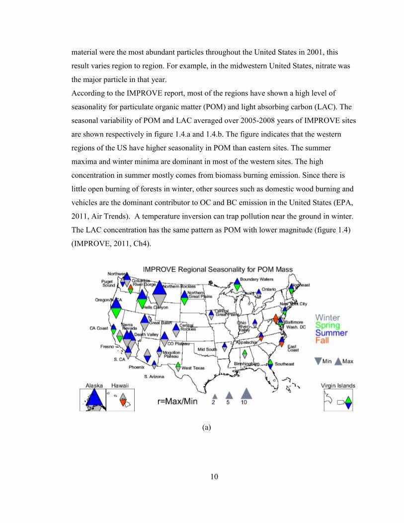
According to the IMPROVE report, most of the regions have shown a high level of

seasonality for particulate organic matter (POM) and light absorbing carbon (LAC). The

seasonal variability of POM and LAC averaged over 2005-2008 years of IMPROVE sites

are shown respectively in figure 1.4.a and 1.4.b. The figure indicates that the western

regions of the US have higher seasonality in POM than eastern sites. The summer

maxima and winter minima are dominant in most of the western sites. The high

concentration in summer mostly comes from biomass burning emission. Since there is

little open burning of forests in winter, other sources such as domestic wood burning and

vehicles are the dominant contributor to OC and BC emission in the United States (EPA,

2011, Air Trends). A temperature inversion can trap pollution near the ground in winter.

The LAC concentration has the same pattern as POM with lower magnitude (figure 1.4)

(IMPROVE, 2011, Ch4).

(a)

11

(b)

Figures 1.4 Seasonal variability of IMPROVE 2005-2008 monthly mean POM (a) and LAC (b)

concentrations. The upward triangle corresponds to the season with maximum concentration and the

downward triangle is corresponded to the season with the minimum concentration. The seasons are

identified by different colors. The size of the triangles is determined by the ratio of maximum to minimum

mean concentration (IMPROVE, 2011, Ch4).

Trend analyses are presented over short-term (2000–2008) and long-term (1989–2008)

time periods. The IMPROVE report includes long-term trend for sulfate ion, total carbon

(TC = organic carbon + light absorbing carbon), fine soil, fine mass (FM), coarse mass

(CM), and PM10 concentrations (IMPROVE, 2011, Ch6).We use data from the

IMPROVE network to examine trends of BC and OC in winter in the United States

between 1989 and 2010. Generally, these data indicate decreases in both species over

most of the regions. Trends in OC and BC for shorter periods (2000-2008) support these

decreases as well. For the trend analysis, fifty percent of yearly data was required for any

given site. In addition, trend analysis was performed for sites with complete data for 70%

of the years depending on the time interval (6 out of 9 years for short-term trends and 14

out of 20 years for long-term trends). Also, trends were computed for four seasons

(winter included December, January, February; spring included March, April, May;

12

summer included June, July, August; fall included September, October, November)

(IMPROVE, 2011, Ch6).

Figure 1.5 shows the long-term trend in total carbon (TC) for winter measured by

IMPROVE for the 1989-2010 period. The most important feature of this figure is that the

sites along the western coast have larger negative trends than the eastern part. According

to the IMPROVE report, there are only 50 sites with complete data for this time period.

The figure indicates that the concentration in winter has decreased during these 20 years.

The long-term TC trend for summer is shown in figure 1.6. The figure shows that the

magnitude of the trend in summer is lower than in winter, and there are many sites

showing no significant trends. According to the seasonal concentration report (figure

1.4), maximum concentrations occur in summer in both OC and BC for the majority of

regions in the western United States due to biomass burning emission and minimum

concentrations happen mostly in winter.

Figure 1.5 Long-term (1989-2008) trends of total carbon mass concentrations for winter (% yr-1

)

(IMPROVE, 2011, Ch6).

13

Figure 1.6 Long-term (1989-2008) trends of total carbon mass concentrations for summer (% yr-1

)

(IMPROVE, 2011, Ch6).

Analyzing the short-term trend gives us the opportunity to consider larger number of sites

in comparison with the long-term trend. In addition, there are more sites with complete

data and approximately 50% of these sites exhibit greater trends. The IMPROVE short-

term trend of TC for winter and summer respectively are shown in figure 1.7 and 1.8.

Like the long-term trend, trends corresponding to sites in the western United States are

larger than trends for eastern sites during winter and summer.

This work focuses on the long-term trend of TC for winter (figure 1.5) and tries to

examine the causes of the observed decrease in the trend especially in the western US.

Since wildfire emissions are minimum in winter, the decreasing trend is unlikely to be

explained by them. However, the decreasing trend of carbonaceous aerosol is consistent

with the large decreases in anthropogenic sources throughout the United States (Murphy

et al., 2011). Emission restrictions were enforced in the United States on fossil fuel and

biofuel-based vehicles since the early 1990s (Yanowitz et al., 2000; Ban-Weiss et al.,

2008). Even the remote IMPROVE sites have been strongly affected by vehicle

regulations and reduction in the use of off-road equipment specially during weekends

(Murphy et al., 2008). In addition, the residential wood burning which is a significant

14

contributor to OC and EC emission during the cold season, has been controlled since

1988 by EPA

(http://www.epa.gov/compliance/resources/policies/monitoring/caa/woodstoverule.pdf).

Figure 1.7 Short-term (2000-2008) trends of total carbon mass concentrations for winter (% yr-1

)

(IMPROVE, 2011, Ch6).

15

Figure 1.8 Short-term (2000-2008) trends of total carbon mass concentrations for summer (% yr-1

)

(IMPROVE, 2011, Ch6).

Due to the significant effect of emission changes on carbonaceous aerosol concentration

(Murphy et al., 2011), it is essential to examine the emission inventories in order to find

out the pattern of aerosol changes. The current emission inventory used in the global

chemical transport model (GEOS-Chem CTM) does not represent the observed OC and

BC trend (Leibensperger et al., 2012). In this study, we examined different emission

inventories to compare with the current one used by GEOS-Chem model (discussed in

chapter 2). We looked for an emission inventory which contains the seasonal variation of

OC and BC emitted by domestic wood burning sector. Finally, we used GEOS-Chem

simulations to reconstruct historical carbonaceous aerosol trends from 1989 to 2010 with

an emission inventory which includes the spatial and seasonal distribution of residential

wood burning to evaluate with observed trend (discussed in chapter two).

16

CHAPTER 2

Analysis of Emission Inventories of Carbonaceous Aerosol

2.1 Trend Analysis

I examined the trend of black carbon and organic carbon by using the measured data

from the IMPROVE network. Trend analysis was performed for those sites with

complete data for 14 years or more. Theil regression (Theil, 1950) was used by taking the

median of all slopes between every possible data pair with the concentration data as the

dependent variable and the year as the independent variable (IMPROVE, 2011, Ch6). A

benefit of Theil regression is that the results are less biased by the outliers (IMPROVE,

2011, Ch6). The trend values (percent change per year, %yr-1

) were derived by dividing

the calculated slopes by the median concentrations of each site and multiplying by 100%.

The significance (p value) of the slope was calculated using Kendall tau statistics

(Kendall, 1990) based on the concentration data. Trends with 95% significance (p≤0.05)

were considered statistically significant (IMPROVE, 2011, Ch6).

Figure 2.1 shows the long-term trend of in situ black carbon, organic carbon and total

carbon concentrations (1989-2008) for winter months. No increasing trends for these

species are found in winter. Decreasing trends are greater for sites located along the

western coast than along the eastern coast for black carbon, organic carbon and total

carbon. Decreasing trends in black carbon could be even larger than shown here due to

the change in BC instrumentation.

This study investigates the factors that contribute to the large decreases of black carbon

and organic carbon over the west and seeks to improve the simulation of carbonaceous

aerosol. Currently, there are some discrepancies between the trend of simulation outputs

and observations of BC and OC (Leibensperger et al., 2012).

17

18

Figure 2.1 Long-term (1989-2008) trends (%yr-1

) of black carbon, organic carbon, and total carbon

concentrations (TC = organic carbon + black carbon) in winter months measured by the IMPROVE

network.

Figure 2.2 is a comparison between simulations and observations of the surface

concentration of BC and OC for years 1990, 2000, and 2010 which was studied by

Leibensperger et al., 2012. The observation data (circles) represent in situ concentrations

measured by the IMPROVE network. Observations are averaged values of three-year

periods: 1989-1991, 1999-2001, and 2008-2010. Due to the discontinuity in observations,

first, the seasonal means (DJF, MAM, JJA, SON) of each year were calculated from only

sites in which each season had a minimum of 10 data points. The seasonal means were

then averaged over each period from only sites for which data was available for at least

two of the three years. The GEOS-Chem simulations (background contours) include a

series of two year decadal time slices from 1950 to 2050, wherein the model uses the first

year for initialization and the second for analysis (version 8.01.01; http://geos-chem.org/).

Meteorological data of 2000-2001 collected by NASA Goddard Earth Observing System

(GEOS-4) was used as the input for all the simulations. The simulation data were

19

regridded to 2°× 2.5° horizontal resolution (Leibensperger et al., 2012). Based on the

figure, some trends are common to both observational data and simulation outputs like

the higher concentrations of BC and OC over the Southeastern US than over the Western

US, which mainly come from open fires (Park et al., 2007). However, there are some

discrepancies between the observations and simulation results during these three decades

which cannot be ignored, particularly over the Western region. In order to identify these

differences, I calculated the trend of the observed and simulated data (Fig 2.3). While the

observed BC and OC concentrations decreased respectively by 50% and 34% between

1990 and 2000 throughout the US, the simulated concentrations show a decreasing trend

of only 27% and 16% (Leibensperger et al., 2012).

Figure 2.3 shows the trend of simulated and observed data of BC and OC concentrations

computed using Theil regression for 1990-2010 for annual values (a) and winter months

(b). For observational data, trend analysis was implemented for those sites with complete

data for 14 years or more. It’s obvious in the figure 2.3(a) that the decreasing trend in

observational data is larger than the simulation outputs both for BC and OC (low bias).

While the observed decreasing trend of BC and OC for some sites located in the west is

significant, the simulated decreasing trend is lower for the corresponding sites. The

decreasing trend of BC and OC measurements is larger in winter than the decreasing

trend for the whole year (Fig 2.3(b)). While there is not much difference between the

decreasing trend of winter data and annual data of BC simulations; a higher decreasing

trend is noticeable for annual OC simulation than OC concentration in winter due to the

significant role of biomass burning in OC concentration. A larger decreasing trend is

noticeable in measured concentrations of BC and OC along the Western regions for

winter months than the trend for simulated concentration in the corresponding sites.

Figure 2.4 compares the time series of total BC and OC concentrations measured by

IMPROVE for winter with simulated outputs (Model output from Leibensperger et al.,

2012) averaged over the sites in the west (sites with longitude < -100), far west (sites

with longitude < -115), east (sites with longitude > -100) , and the whole US. The figure

shows that the decreasing trend of the BC and OC observations is much higher than the

20

simulated trend for all the four regions. The trend computed for sites in far west has the

largest decreasing slope, and the simulated output fails to replicate the observed trend.

The spike in the BC data in 2005 may be influenced by the change in BC

instrumentation. The true trend could be even larger.

Figure 2.2 Concentration of black carbon (left) and organic carbon (right) (µg m-3

). The in situ

observations shown by circles are three year averages for 1989-1991, 1999-2001, and 2008-2010. The

background contours represent the outputs of GEOS-Chem simulations for 1990, 2000, and 2010 emissions

(Leibensperger et al., 2012).

21

Figure 2.3 A comparison of the trend of simulation outputs with observations calculated using Theil

22

regression for 1990-2010 for annual data (a) and for winter months (b).

2.2 Bottom-up emission inventories of BC and OC

Murphy et al., 2011 discussed how the changes in emissions from the United States have

a major impact on carbonaceous aerosol concentrations; therefore, it is necessary to

inspect the trend of the available emission sources to find the causes of the observed

decreasing trend. Wild fire emissions are unlikely to be a major factor for the observed

decline, because the role of open fires in BC and OC emissions are the least in winter

months. In this regard, I focused on anthropogenic emissions of BC and OC. Controls on

fossil fuel and biofuel emissions have been implemented since 1990s and appear to be

responsible for the decreasing trend of carbonaceous aerosols (Murphy et al., 2011;

Yanowitz et al., 2000; Ban-Weiss et al., 2008). However, most of these restrictions are

constant during a year. Since domestic wood burning is an important source of

carbonaceous aerosol (Rogge et al., 1991), and due to the strong correlation between the

decrease in black carbon and organic carbon concentrations and the controls on wood

stoves since 1988 (Murphy et al., 2011), I suspected that the observed trend in BC and

OC are due to the decrease of this source. According to a trend study provided by NEI,

the wood consumption in residential sector has decreased by a factor of 2 during 1985-

2000 (appendix A). Since the use of fireplaces and woodstoves are maximum in winter,

the reduction in residential emission would be the dominant factor responsible for the

observed decrease in BC and OC concentrations. I searched for available emission

inventories which contained the seasonal variations of carbonaceous aerosol emitted by

wood burning. The emission inventory which is currently used in GEOS-Chem model

(Bond et al., 2007) is unable to well represent the observed BC and OC trend

(Leibensperger et al., 2012). According to figure 2.4, the Bond emission inventory does

not well reproduce the winter time trends in carbonaceous aerosols. I evaluated other

available inventories (Lamarque [RCP database] and MACCity inventory) to examine

their accuracy. Since I focused on winter months, I considered biofuel and fossil fuel

emissions and did not include open fire emissions.

23

Figure 2.4 A comparison of the winter (DJF) time series of the observed (IMPROVE measurements) and

GEOS-Chem model output from Leibensperger et al. (2012) averaged over sites in the west, far west, east

and the whole US for black carbon and organic carbon (µg m-3

).

24

The Bond emission inventory (Bond et al., 2007) is the default for GEOS-Chem

simulations. Figure 2.5 (a) presents the spatial distribution of annual black carbon (left)

and primary organic carbon emissions (right) estimated by Bond emission inventory

(http://www.hiwater.org/) for years 1980, 1990, and 2000 (kg/m2/s). These 1° × 1° data

include emissions from fossil fuel and biofuel combustion, and do not contain any open

vegetative burning emissions (e.g. forests or savanna). Fuel-use data include power

generation, industry, transportation and residential sectors (Bond et al., 2007).

Figure 2.5b shows the trend of emissions for these three decades using the Theil

regression method. BC and OC emissions declined over the western regions less than

over the eastern parts of North America during 1980-2000. The total emission of BC has

decreased by 12% during 1990-2000 throughout North America which is about 4%

reduction in BC emission over the west, and 16% over the east of North America for

1990-2010. Also, the total OC emission has decreased by 16% in North America in the

same period (Bond et al, 2007). The decrease in OC emission is about 7% and 19%

respectively over the western sites and eastern regions (see Table 2.1).

Figure 2.6 (a) presents the spatial distribution of annual black carbon (left) and primary

organic carbon emissions (right) estimated by Lamarque emission inventory (RCP

database) (http://www.iiasa.ac.at/web-apps/tnt/RcpDb) for the years 1980, 1990, and

2000 (kg/m2/s). The RCP emission inventory is a combination of Bond et al. (2007) and

Junker and Liousse (2008). These 0.5° × 0.5° data include anthropogenic emissions of

domestic, energy, industry, transportation, and agricultural waste burning sectors. Also,

these data do not contain biomass burning emissions. The trend of BC and OC emissions

are shown in Figure 2.6 (b) for 1980-2000. More locations are apparent with increasing

trends of BC emissions especially over the Southwestern US which are not seen in the

computed trend of Bond emission inventory. Also, there are more parts in the Eastern

US with decreasing trends of BC emission. The trend in OC emission is similar to the

trend of OC in Bond inventory. The RCP database represents the reduction in BC

emission during 1990-2000 by about 6% throughout North America, 1% over the west

and 9% over the east of North America. The decrease in OC emission over North

25

America, western and eastern regions of North America is respectively estimated about

14%, 4%, and 17% (see Table 2.1).

Figure 2.5 Spatial distribution of black carbon (left) and organic carbon (right) (kg/m2/s) emitted by fossil

fuel and biofuel combustion in 1980, 1990, and 2000 over North America (Bond et al., 2007) (a). The

estimated trend of black carbon (left) and organic carbon (right) emissions (kg/m2/s/year) by using Theil

regression for 1980-2000 (b).

26

Species Sector Database 1980 1990 2000 2010

BC West Bond 0.14 0.14 0.14 -

BC East Bond 0.32 0.34 0.29 -

BC NA Bond 0.46 0.48 0.42 -

BC West RCP 0.14 0.14 0.14 -

BC East RCP 0.40 0.37 0.34 -

BC NA RCP 0.53 0.51 0.48 -

BC West MACCity - 0.14 0.14 0.10

BC East MACCity - 0.37 0.34 0.20

BC NA MACCity - 0.51 0.48 0.31

OC West Bond 0.22 0.20 0.19 -

OC East Bond 0.62 0.53 0.43 -

OC NA Bond 0.85 0.74 0.62 -

OC West RCP 0.23 0.22 0.21 -

OC East RCP 0.69 0.58 0.48 -

OC NA RCP 0.92 0.81 0.70 -

OC West MACCity - 0.24 0.23 0.18

OC East MACCity - 0.59 0.50 0.32

OC NA MACCity - 0.83 0.73 0.50

Table 2.1 Total values of BC and OC emission (Tg/yr) estimated by three emission inventories (Bond,

RCP, and MACCity) and averaged over North America, West, and East of North America for years 1980,

1990, and 2000.

The MACCity inventory offers monthly global gridded BC and OC emissions. MACCity

anthropogenic emissions are derived from the ACCMIP and RCP8.5 datasets. Figure 2.7

displays the seasonal trend of black carbon (top) and organic carbon emissions (bottom)

projected by MACCity emission inventory with the use of Theil regression for years

1990-2010 (available at http://eccad.sedoo.fr/eccad_extract_interface/). These 0.5° × 0.5°

data include anthropogenic emissions of domestic, energy, industry, transportation, and

agricultural waste burning sectors. The seasonal variation of MACCity anthropogenic

emissions was developed as part of the RETRO project. Within RETRO, seasonal

27

variations were defined for different sectors. The same seasonal variation for each sector

was used for all years, since no data exist concerning possible changes to seasonal

variation in emissions during the past decades. It is evident in the figure that the

decreasing trend is the largest for winter for both BC and OC emissions. The decrease in

BC and OC emissions are higher in eastern part than western region.

In order to evaluate the available emission inventories, I calculated the trend using Theil

regression for each emission inventory including Bond, Lamarque, and MACCity. I

examined trends in North America between 1990 and 2000. For observational data, I

considered sites with available data for 7 years or more. Figure 2.8 compares the trends

of annual emissions (kg/m2/s/year) (left) and concentrations (µg/m

3/year) (right) of black

carbon and organic carbon in winter for 1990-2000. Since anthropogenic emissions are

the main source of carbonaceous aerosol in cold months, I didn’t include open burning

emissions in my comparisons. A large decreasing trend in BC concentrations is apparent

along the Northwestern United States which is not correlated with a large decrease in BC

emission of any of the mentioned emission inventories over this region. While the Bond

inventory indicate a decreasing trend in the Southwestern US corresponded to the

observed decline in BC concentrations, the decreasing trends estimated based on

Lamarque and MACCity inventories have smaller values with a handful sites showing

increasing trend. Overall, while there is a small decrease in concentration along the west

coast, no trend is observed in BC emissions for all the three emission databases. The

similar pattern with higher magnitude holds for OC as well.

Since emissions and concentrations are not exactly of the same nature, therefore they are

not directly comparable. For better comparisons, I calculated the percent change per year

of both emissions and concentrations. I computed the percentage trends of emissions

weighted by the median emission over the 1990-2000 decade and multiplied by 100%. I

used the same way for the IMPROVE data; the slopes, calculated by the Theil regression

method, were divided by the median concentration of the 1990-2000.

28

Figure 2.6 The Map of black carbon (left) and organic carbon (right) emissions from fossil fuel and biofuel

combustions derived from Lamarque inventory in 1980, 1990, and 2000 (kg/m2/s) over North America

(Lamarque et al., 2010) (a). The calculated trend of black carbon (left) and organic carbon (right) emissions

(kg/m2/s/year) based on the Theil regression method for 1980-2000 (b).

29

Figure 2.7 The seasonal trend of black carbon (top) and organic carbon (bottom) emissions (kg/m2/s/year)

of MACCity inventory estimated by using Theil regression for 1990-2010 (Lamarque et al., 2010).

Figure 2.8 The comparison of the trends of BC and OC annual emissions (kg/m2/s/year) (left) with the

trends of surface concentrations of BC and OC (µg/m3/year) for winter (right). The trends are computed by

applying the Theil regression method for 1990-2000.

30

Figure 2.9 represents the resulting trend of emissions and concentrations. Based on the

figure, the averaged decrease in BC concentration is about 6% per year all along the

western coast during the 1990-2000. The highest reduction in BC emission is about 4%

decrease per year on average observed in the south western US for all the three emission

inventories. There are some sites showing small decrease in emission over North western

US derived from Bond inventory. The figure also shows 8% reduction (on average) in

OC concentration specially for the sites located in the west and North west. However, a

large reduction in emission (4% on average) over the western coast is apparent for all the

mentioned emission inventories. The reduction in OC emission based on the Bond

emission inventory is more correlated to the observed decrease in concentration than RCP

and MACCity databases over the north western region.

Figure 2.9 A comparison of the trend of annual emissions (left) with the trend of surface concentrations of

BC and OC (%year-1

) for winter (right) for 1990-200 The grey color indicates the region with small

emission values which can be ignored.

31

Based on the comparisons, the pattern of the emission changes was not correlated with

the observed trend of BC and OC concentrations for 1990-2000 decade. Since my main

concern was the trend in winter months, having an emission inventory with the seasonal

variation of residential wood burning would be helpful. Unfortunately, none of the

mentioned emission inventories included the seasonal change of wood burning. The need

to find a suitable emission inventory that would provide the seasonal variation of

domestic wood burning led me to develop a database by modifying the available

emission inventories. For this purpose, I used the global sectoral emission inventory for

the Arctic Research of the Composition of the Troposphere from Aircraft and Satellites

project (ARCTAS). The base year is 2006, and the resolution is 0.5 × 0.5 degree divided

into four sectors: residential, industry, power, and transport. Also, I used the sectoral

trends of Argonne National Laboratory (ANL) for North America during 1995-2010

(http://www.anl.gov/). The ANL collected values of black carbon and organic carbon

emissions from residential, industry, power, transport, open burning of forest& savannah

and open burning of agricultural waste. In order to focus on the anthropogenic impact, I

excluded the two last sectors of ANL values from the total. The sectoral information in

the ARCTAS inventory is not consistent with the sectoral trends of ANL for North

America. The sectoral ARCTAS inventory of North America is developed based on

information from multiple sources, including NEI, CAC, Bond et al., (2007), and

AEROCOM inventory. Therefore, there are some discrepancies between ARCTAS and

ANL data. To avoid these discrepancies, I scaled all the ANL values by sector to match

the ARCTAS value for the year 2006.

Since the ANL data did not provide the spatial distribution, I projected the ANL trend

values for each sector onto the 2006 (ARCTAS data) spatial distribution of that source.

This allowed estimation of the spatial distribution of OC and BC emissions for 1995-

2010.

I used the historical inventory developed by Lamarque et al. 2010 for years prior to 1995.

I had data values for years: 1980, 1990 and 2000. I estimated the values for other years

by assuming a linear trend between years: 1985:1990 and 1990:1995. To merge the

32

Lamarque and ANL data, I scaled all the estimated values for years 1985-1995 by a scale

factor needed to match the total anthropogenic emission of ANL for 1995. I estimated the

spatial distribution of each sector related to years 1985-1995 from the Lamarque data the

same way I derived the map for the ANL data based on the year 2006 of ARCTAS.

I represented the seasonal variation of the residential sector as a cosine function with a

maximum during January and minimum during July. I assumed that the seasonal

variations of the other sectors (industry, power and transport) are small enough to be

ignored. Since the trend values were different for the US and Canada, all calculations

were done separately and resulting values for these two regions were combined.

Figure 2.10 represents the time series of the anthropogenic emissions over North America

during 1995-2010. It compares the new database with ANL and different sectors of the

new database for BC and OC. The figure shows the important contribution of the

transport sector in BC emission, and the residential sector in OC emission in this time

interval over North America.

Figure 2.11 represents the seasonal and spatial distribution of black carbon (top) and

organic carbon (bottom) emissions (kg/m2/s) of the new database for the year 2006. The

largest BC and OC emissions are in winter due to residential wood burning.

The absolute emission of black carbon for residential, industry, power, and transport

sectors (kg/m2/s) derived from the new database for years 1990, 2000, and 2010 are

shown in figure 2.12. The figure implies that the total BC emission has decreased by

about 21% between 1990 and 2010 in the residential sector. This decrease is not obvious

on the west. There is 0.6% increase in BC emission in the industry sector, and 17%

decrease in BC emitted by the power sector over this time period. The transport section

plays a major role in overall reduction of BC emission ( 44%) as a result of restrictions

on diesel engines enforced since 1990s (Murphy et al., 2011). In addition, this decrease is

particularly noticeable along the western regions. The total BC emissions for these three

decades are included in table 2.2.

33

Figure 2.10 The time series of North American emissions (the new database, and the ANL database)

(kg/year) for 1995-2010 for BC and OC.

34

Figure 2.11 Seasonal and spatial distribution of black carbon (top) and organic carbon (bottom) emissions

(kg/m2/s) for the year 2006 over North America derived from the new database.

Year Residential Industry Power Transport Total

1990 0.08 0.06 0.01 0.17 0.31

2000 0.07 0.06 0.01 0.14 0.27

2010 0.06 0.06 0.00 0.09 0.22

Table 2.2 Total emission values of black carbon (Tg/yr) for years 1990, 2000, and 2010 derived from the

new database.

Figure 2.13 shows the trend of each sector (residential, industry, power, and transport) of

the new emission database (kg/m2/s/year) for 1990-2010 calculated using Theil

regression. The figure indicates that the BC emitted by the transport sector has been

decreased in this period. We have the same trend in the residential sector but with lower

rate. Both of these two sectors have reduced over western regions. Emissions from the

power and Industry sectors have small increases during 1990-2010.

35

Figure 2.12 Spatial distribution of black carbon emission for years 1990, 2000, and 2010 for four different

sectors (residential, industry, power, and transport) (kg/m2/s) derived from the new database throughout

North America.

The fractional change of different sectors (residential, industry, power, and transport) for

years 1990, 2000, and 2010 of the new database (%) is presented in figure 2.14. The

figure indicates the percentage that each sector contributes to the total anthropogenic

emission of BC. Overall, the residential sector contributed only 25-30% on average,

while the transport sector had a significant impact on BC emission, around 55-90%

during 1990-2010. The industry and power sectors had smaller roles respectively, about

36

Figure 2.13 The trend of black carbon emission for different sectors (residential, industry, power, and

transport) (kg/m2/s/year) estimated by the new database for 1990-2010.

20-30% and 0-20%. It is evident in the figure that the transport sector is the most

dominant factor in BC emission in the Western US, and the residential sector contributes

20% of the total anthropogenic emission on average over this region. The sharp change in

fractional emission between Canada and US can be explained by the diffrenet methods in

combinaing data in Canada and the US.

Figure 2.15 shows the absolute emission of organic carbon for different sectors

(residential, industry, power, and transport) (kg/m2/s) for years 1990, 2000, and 2010.

The total OC emitted by the residential sector has decreased by about 34% between 1990

and 2010 over North America. While the OC emission has reduced by about 23% in the

37

industry sector in this time period, there is an increase in the OC emission by about 0.5%

in the power sector. The transport sector has contributed to the reduction in OC emission

by about 52%. Based on the figures, the transport sector and the residential sector are

particularly responsible for the decrease in OC concentrations along the western regions.

Table 2.3 presents the total OC emissions for these three decades.

Figure 2.14 Spatial distribution of the fraction of each sector of black carbon emission for years 1990,

2000, and 2010 (%) derived from the new database. The values written in the figure are the total black

carbon absolute emission for each year

38

Year Residential Industry Power Transport Total

1990 0.36 0.04 0.01 0.10 0.50

2000 0.28 0.04 0.01 0.07 0.39

2010 0.24 0.03 0.01 0.05 0.32

Table 2.3 Total emission values of organic carbon (Tg/yr) for years 1990, 2000, and 2010 derived from

the new database.

Figure 2.15 Spatial distribution of organic carbon emission for years 1990, 2000, and 2010 for four

different sectors (residential, industry, power, and transport) (kg/m2/s) estimated by the new database

throughout North America.

39

Figure 2.16 represents the trend analysis of each anthropogenic sector (residential,

industry, power, and transport) for OC emission (kg/m2/s/year) for 1990-2010. The

residential and transport sector have the same decreasing trend in OC emission during

this period. The residential sector has the higher effect particularly on the western US.

The emission of OC by the industry sector has a lower decreasing trend; also, the

increasing trend of the power sector has significantly lower rate in this period.

Figure 2.16 The trend of organic carbon emitted from different sectors (residential, industry, power, and

transport) (kg/m2/s/year) derived from the new database for 1990-2010.

Figure 2.17 presents the percentage of the contribution of each sector (residential,

industry, power, and transport) in OC anthropogenic emission of each grid for years

1990, 2000, and 2010 of the new database (%). According to the figure, the residential

40

sector had a significant influence on OC emission, about 50-70% on average, while the

transport sector had a weaker impact (20-40%) during 1990-2010. The industry and

power sectors had smaller roles respectively, about 0-10% and 0-20%. The figure

indicates that the residential sector is the dominant factor in the anthropogenic production

of primary OC over the western US.

Figure 2.17 Spatial distribution of the fraction of each sector of organic carbon emission for years 1990,

2000, and 2010 (%) derived from the new database. The total organic carbon absolute emission values are

written for each year.

41

2.3 Inventory Evaluation

After combining the new database, I used GEOS-Chem chemical transport model version

v9-01-02 (Bey et al., 2001) (www.geos-chem.org) to reproduce the observed BC and OC

surface concentrations. The simulations were directed for a series of four months

(November, December, January, and February). I used one month (November) for spin

up, and the simulations were completed for winter months of years 1989, 1995, 2000,

2005, and 2010 (for example: Nov 1994-Feb 1995). The same meteorological data 2004-

2005 from the NASA Goddard Earth Observing System (GEOS-5) were used by all the

simulations. The GEOS-5 met fields (data) used in this study included 72 vertical layers,

6-hour of temporal resolution (3-h for surface variables), and 0.5° latitude by 0.667°

longitude horizontal resolution which were regridded to 2°×2.5° horizontal resolution for

input to GEOS-Chem.

The simulation of carbonaceous aerosols in GEOS-Chem followed the scheme used by

Liao et al., 2007 and Park et al., 2006 with some adjustments of emission inventories

described below. The model used Bond emission inventory (Bond et al., 2007) as the

global anthropogenic emissions of BC and POA (fuels). The mentioned emission source

of BC and POA was replaced by the new database only for North America. The model

applied the scheme used by Park et al., 2006 for SOA formation which involved the

semi-volatile oxidation products from biogenic terpenes, biogenic isoprene, and

aromatics, as well as the irreversible uptake of glyoxal and methylglyoxal. As in Park et

al. (2003), the carbonaceous aerosol simulation is based upon the assumption that 80% of

hydrophobic EC and 50% of hydrophobic OC could be attributed to primary emission

sources which can convert to hydrophilic aerosols by an e-folding time of 1.2 days

[Cooke et al., 1999; Chin et al., 2002; Chung and Seinfeld, 2002], and all SOA is

assumed to be hydrophilic (Park et al., 2003). In addition, the monthly mean emission

source of biomass burning was driven from the GFED2 inventory with 8-day resolution

(van der Werf et al., 2009).

42

The model followed Liu et al. (2001) for the simulation of aerosol wet and dry

deposition. Wet deposition took into account processes such as scavenging in convective

updrafts, rainout and washout (Park et al., 2003).

Figure 2.18 presents the simulation outputs for these years for BC and OC

concentrations. We compared the model results against the observed BC and OC

concentrations (µg/m3). Observations are three year averages of winter months for 1988-

1990, 1994-1996, 1999-2001, 2004-2006, and 2008-2010 measured by the IMPROVE

network. The IMPROVE measurements are gridded to the 2°× 2.5° model grid. The

higher observed concentrations of BC and OC in the eastern US than in the western part

imply the larger role of anthropogenic emission in the east (Park et al., 2003). It is

evident in the figure that, the model doesn’t well capture the spatial distribution of BC

and OC concentrations. While observed concentrations of BC and OC show highest

values in the Southeast of the US, the model shows maximum concentrations over North

eastern United States. For western regions, the model outputs of BC and OC follow

similar patterns in spatial distribution as the observations, but with major differences in

magnitude (low bias).

We also computed the site-to-site comparisons between model and observations of

carbonaceous aerosol (Figure 2.19). The figure shows there are some major differences

between the model outputs and observations. The model underestimated both BC and

OC concentrations at some sites in the Western coast and especially over the south

eastern US. Overall, the model captured the observed values of black carbon

concentration in remaining sites; however, the model underestimated OC concentration at

almost all rural sites.

In addition, I computed the fractional trend of simulation outputs using Theil regression

(for winter time of years: 1989, 1995, 2000, 2005, and 2010), and compared with the

observed trend of BC and OC concentrations (%yr-1

) for winter time (DJF) of 1989-2010.

Figure 2.20 compares the simulated and observed trend of BC and OC concentrations

during this time period. As seen in the figure, there are major differences between the

observed and simulated trend. While the model overestimated the observed decreasing

43

trend of BC concentration for a few sites located at the Western coast, it underestimated

the decreasing trend of OC concentrations in this region.

Figure 2.18 A Comparison of simulation outputs with the observations of BC and OC surface

concentrations (µg/m3)

in winter. Observations are three-year averages for 1988-1990, 1994-1996, 1999-

2001, 2004-2006, and 2008-2010 measured by IMPROVE. GEOS-Chem model outputs are derived from

winter time simulation for 1989, 1995, 2000, 2005, and 2010.

Given the discrepancies between the simulated and observed trend, the new database

seems inadequate to improve the representation of BC and OC concentrations. Therefore,

I explored alternative techniques.

44

Figure 2.19 The difference between the simulation outputs and observations for black carbon (top panel)

and organic carbon (bottom panel) for winter season of the years 1989, 1995, 2000, 2005, and 2010.

Figure 2.20 A comparison between the observed and simulated trend of BC and OC concentrations by

using Thiel regression. The simulated trend is calculated for winter season of the years 1989, 1995, 2000,

2005, and 2010. The observed trend is computed for winter season of 1989-2010 (%year-1

).

45

2.4 “Top-down” Estimate of Anthropogenic Sources

I applied multiple linear regression (Brown et al., 2009) to examine the changes in

emission sources which minimize the differences between the simulation and

observations. In this regard, the anthropogenic emission sectors I considered were

residential, industry, power, and transport. In order to find a relation between each

emission sector and carbonaceous aerosol concentration, I reduced each emission sector

by 10% as a perturbation and conducted the simulation by having the reduction in each

specific sector and having other sectors constant. The perturbed simulations were

conducted for 3 different years: 1995, 2000, and 2005. Since domestic wood burning

practices vary regionally, I divided the residential emission sector into western and

eastern regions (separated at 100° W). The following equation represents the relationship

of the change in simulated concentration (∆Cmod) as a function of changes to five

different emission factors (Ek,i): residential emission in the west (k=ResWest), residential

emission in the east (k=ResEast), industry (k=Ind), power (k=Pwr) and transport

(k=Trans) sectors.

∆Cmod,i = β0 + β1 EResWest,i Cmod,i (2nd

-1st) / ∆EResWest,i + β2 EResEast,i

Cmod,i (2nd

-1st) / ∆EResEast,i + β3 EInd,i Cmod,i (2

nd-1

st) / ∆EInd,i

+ β4 EPwr,i Cmod,i (2nd

-1st) /∆EPwr,i+ β5 ETrans,i Cmod,i (2

nd-1

st) /∆ETrans,i (eq. 3.1)

The subscript, i, represents the group of IMPROVE sites in each grid box and β0

represents the background concentration of carbonaceous aerosols.The scale factor for

each anthropogenic emission sector including residential emission in west, residential

emission in east, industry, power, and transport are respectively determined by β1, β2, β3,

β4, and β5. The Cmod,i (2nd

-1st) indicates the average difference in model output

concentration of the second and first simulation for 1995, 2000, and 2005. The ∆Ek,i

refers to the 10% reduction in each specific sector (k, ResWest, ResEast, Ind, Pwr,

Trans). Since ground-level OC and BC concentrations are driven strongly by local

emission sources (Park et al., 2003), I ignore the background concentration for these

calculations (β0 = 0).

46

I used multiple linear regression analysis (Brown et al., 2009) to calculate the least square

of the cost function which is the difference between the simulated and observed trend. I

calculated the optimum values for scale factors of each emission sector while the cost

function is the minimum. The cost function (J) is described by the following

relationship: J = ∑ (∆Cmod,i –∆Cobs,i)2

(eq. 3.2)

I created a matrix (C) which contained the emission perturbations for each sectors in its

columns (Χij). Based on the following equation, I computed the optimum scale factors

which minimize the difference between the observed trend (D is a vector containing the

trend of the BC and OC concentrations at N sites) and the simulated trend which will be

derived by multiplying matrix C by the coefficients vector (B is a vector containing Κ=5

scale factors for emission sectors (residential, industry, power, and transport)).

The vector D has length 2N since it contains both BC and OC observations. I

normalized the BC and OC values by their mean concentration in winter for 1989-2010 to

give equal weight to BC and OC concentrations in the least square computations (0.16 µg

m-3

for BC, and 0.53 µg m-3

for OC). The trends ∆Cobs,i were computed based on Theil

regression. Therefore, the resulting coefficients in B determine the changes in emission

sectors which lead to the minimization of the bias between observed and simulated trend

of BC and OC concentration in winter.

Table 2.4 shows the resulting trends. The computed values present the percent change in

emission sectors which should be implied in order to minimize the current differences

between the observed and simulated trend. I found that the residential sector should have

(eq. 3.3)

47

a decreasing trend with similar magnitude in the west and east during 1989-2010 in North

America. Also, the decreasing trend of transport emissions is almost twice as large as

residential during this time interval. The large trend in transport emissions is supported

by Schauer and Cass et al., 2000. Figure 2.21 presents the comparison between the

simulated and observed trend (a) with the initial guess for the emission scale factors (an

assumption that the scale factor for all emission sectors are 1), and (b) with the scale

factors derived from the least square calculation. As shown in the figure, the difference

of the observed trend and simulated trend is decreased significantly when the coefficients

calculated by linear regression are applied.

Sectors β (unitless)

Residential West -0.035

Residential East -0.039

Industry 0.056

Power 0.084

Transport -0.067

Table 2.4 The scale factors computed based on multiple linear regression for different sectors (residential

west, residential east, industry, power, and transport).

According to the computed coefficients, the observed decreasing trend of BC and OC is

driven by a combination of factors particularly reduction in residential and transport

emission. Apparently, the controls on the use of diesel engine vehicles, fireplaces and

residential stoves applied since 1990s have a significant contribution to the decreasing

trend of carbonaceous aerosols (Murphy et al., 2011). These modifications are different

to fit site-specific discrepancies of observed and simulated trend due to local sources, and

geographic characteristics.

I compared the fractional trend (%year-1

) of the BC and OC observations with the

modified simulated trend for winter time of 1989-2010 (figure 2.22). The figure

indicates that the decreasing trend derived from the modified simulation is smaller at

most western sites for both BC and OC concentrations; overally the modified trend better

reproduced the observed trend in comparison with bottom-up inventories.

48

Figure 2.21 A comparison of the observed trend with the simulated trend derived from (a) initial guess of

emission scale factor (b) the optimized scale factors (µg m-3

year-1

) for BC and OC during winter time of

1989-2010. The third column shows the difference of the observed and simulated trend. The root mean-

square deviation is calculated for each case.

49

Figure 2.22 A comparison between the observed trend in BC and OC concentrations (%year-1

) with the

resulting simulated trend for winter 1989-2010.

It is interesting that the absolute trends in residential sources are similar in the east and

west. The larger relative trend in the west appears to be driven by the large relative

effects of residential and traffic sources to this region. Industry and power has larger roles

in the east.

50

CHAPTER 3 CONCLUSION

3.1 Summary

The large impact of carbonaceous aerosols (black carbon (BC) and organic carbon (OC))

on human health and Earth’s climate implies the importance of understanding the factors

affecting their variations. A trend analysis, using observations from the IMPROVE

network, indicated a large decreasing trend in surface black carbon and organic carbon

concentrations at nonurban sites in winter months during 1989-2010 over North America.

The larger relative negative trend in the western region than the eastern region aroused

curiosity about the causes of the observed trend. Since the lifetime of carbonaceous

aerosols is short (days), the changes in BC and OC emissions can significantly affect

their concentrations. Therefore, an investigation of the changes in anthropogenic

emissions of carbonaceous aerosols could be helpful to understand the causes of the

observed pattern. The role of biomass burning and open fire was not considered in this

work, because open fire is minimum in winter time. The use of domestic wood burning

(wood burning intended for cooking and heating) which contributes mainly to OC and

BC emissions in winter has been controlled since early 1990s. This work examined the

role of the decrease in the residential emission sector on the observed negative trend

particularly over the west. Since the emissions from the residential sector change strongly

with seasons, an emission inventory which contained the seasonal variation of residential

emission sector would be helpful. None of the evaluated emission inventories had this

feature.

A chemical transport model (GEOS-Chem) was used to relate emissions of carbonaceous

aerosols to concentrations that could be evaluated versus IMPROVE observations. The

comparison of the trend of available anthropogenic emission sources (including Bond,

Lamarque, and MACCity) with the observed trend of carbonaceous aerosols evaluated

the accuracy and reliability of the bottom-up emission inventories. The failure to find a

suitable emission inventory which presented a similar trend in emission sources as

51

observed in the trend of BC and OC concentrations at corresponding sites led this work to

combine data based on the emission values of two different databases (ARCTAS and

ANL), and applying a seasonal change for residential sector. Nonetheless, the simulated

output driven by the new database also underestimated the observed trends in BC and OC

concentrations.

Since the new database was not able to represent the observed trend, a multiple linear

regression method was used by this work to derive the constraint of emission sectors. The

top-down emission approach assessed the impact of anthropogenic emission sources

(including residential, industry, power, and transport) quantitatively over North America.

Based on the computed scale factors, the large relative changes in residential and

transport sectors mainly contribute to the larger relative observed trend in the west of the

United States. The calculated coefficients indicate a similar absolute trend in residential

sectors originated from the west and east of the US. Industry and power have larger

effects in the east.

However there are still some discrepancies between the observed and the simulated trend

which need to be resolved. For example, the model overestimates the trend over the south

eastern regions which cannot be eliminated. Therefore, further investigations needs to be

done for the changes that these calculations have implied.

3.2 Future Directions

Discrepancies remain between the resulting simulated trend and the observed trend of BC

and OC concentrations. These discrepancies could reflect inadequacies of using linear

regression to modify an entire sector. Applying the adjoint model could be helpful to

resolve the spatial patterns of carbonaceous aerosols. Also, further collaboration with

bottom-up inventory developers may help to improve the current emission databases and

understand the observed BC and OC trend. In addition, further study on the trend in

carbonaceous aerosol deposition and the pattern of their mixing process particularly over

the western coast could be helpful in this regard.

52

BIBLIOGRAPHY

Albrecht, B. (1989), Aerosols, cloud microphysics, and fractional cloudiness, Science,

245, 1227 – 1230, doi:10.1126/science.245.4923.1227.

Argonne National Laboratory (ANL). (http://www.anl.gov/).

Ban-Weiss, G. A., McLaughlin, J. P., Harley, R. A., Lunden, M. M., Kirchstetter, T. M.,

Kean, A. J., Strawa, A. W., Stevenson, E. D., and Kendall, G. R.: Long-term changes in

emissions of nitrogen oxides and particulate matter from on-road gasoline and diesel

vehicles, Atmos. Environ., 42, 220–232, 2008.

Bey, I., D. J. Jacob, R. M. Yantosca, J. A. Logan, B. Field, A. M. Fiore, Q. Li, H. Liu, L.

J. Mickley, and M. Schultz, Global modeling of tropospheric chemistry with assimilated

meteorology: Model description and evaluation, J. Geophys. Res., 106, 23,073–23,096,

2001.

Bond, T.C., Streets, D.G., Yarber, K.F., Nelson, S.M., Woo, J.-H., Klimont, Z., 2004. A

technology-based global inventory of black and organic carbon emissions from

combustion. Journal of Geophysical Research 109, D14203.

Bond, T.C. et al, Historical emissions of black and organic carbon aerosol from energy-

related combustion, 1850-2000, Global Biogeochem. Cycles, 21, GB2018, doi:

10.1029/2006GB002840, 2007.

Bond emission inventory. (http://www.hiwater.org/).

Brown, S.H. et al, Multiple Linear Regression Analysis: A Matrix Approach with

MATLAB. Alabama Journal of Mathematics, Spring/Fall 2009.

Cabada, J. C., Pandis, S. N., and Robinson, A. L. (2002a). Sources of Atmospheric

Carbonaceous Particulate Matter in Pittsburgh, Pennsylvania, J. Air Waste Manag.

Assoc. 52:732–741.

Cavalli, F., Viana, M., Yttri, K. E., Genberg, J., and Putaud, J.-P.: Toward a standardised

thermal-optical protocol for measuring atmospheric organic and elemental carbon: the

EUSAAR protocol, Atmos. Meas. Tech., 3, 79–89, doi:10.5194/amt-3-79-2010, 2010.

Chow, J. C., Watson, J. G., Pritchett, L. C., Pierson, W. R., Frazier, C. A., and Purcell, R.

G.: The DRI thermal/optical reflectance carbon analysis system: Description, evaluation

and applications in US air quality studies, Atmos. Environ., 27A, 1185–1201, 1993.

53

Chow, J. C., Watson, J. G., Chen, L.-W. A., Chang, M. C. O., Robinson, N. F., Trimble,

D., and Kohl, S.: The IMPROVE A temperature protocol for thermal/optical carbon

analysis: maintaining consistency with a long-term database, J. Air Waste Manage.,

57, 1014–1023, 2007.

Cooke, W.F., Liousse, C., Cachier, H., Feichter, J., 1999. Construction of a 11_11 fossil

fuel emission data set for carbonaceous aerosol and implementation and radiative

impact in the ECHAM-4 model. Journal of Geophysical Research 104, 22,137–22,162.

Dockery, D.W.; Pope, C.A., III; Xu, X.; Spengler, J.D.; Ware, J.H.; Fay, M.E.; Ferris,

B.G.; Speizer, F.A. An Association between Air Pollution and Mortality in Six U.S.

Cities; N. Engl. J. Med. 1993, 329, 1753-1759.

Forster, P., Ramaswamy, V., Artaxo, P., Berntsen, T., Betts, R., Fahey, D. W., Haywood,

J., Lean, J., Lowe, D. C., Myhre, G., Nganga, J., Prinn, R., Raga, G., Schulz, M., and Van

Dorland, R.: Radiative Forcing of Climate Change, in Climate Change 2007: The

Physical Science Basis. Contribution of Working Group I to the Fourth Assessment

Report of the Intergovernmental Panel on Climate Change, edited by S. Solomon, D. Qin,

Kendall, J. (1990). Principles of Good Practice in Combining Service and Learning. in

Combining Service and Learning: A Resource Book for Community and Public

Service Vol. I, National Society for Internships and Experiential Education, Raleigh,

N.C.: NSIEE.

Gray, H.A., Cass, G.R., Huntzicker, J.J., Heyerdahl, E.K., Rau, J.A., 1984. Elemental and

organic carbon particle concentrations: a long term perspective. Science of Total

Environment 36, 17-25.

IMPROVE Report (2011).

http://vista.cira.colostate.edu/improve/Publications/Reports/2011/2011.htm

IPCC, Climate Change 2001: The Scientific Basis, Ch. 6, 2007.

Kendall, J. (1990). Principles of Good Practice in Combining Service and Learning.

in Combining Service and Learning: A Resource Book for Community and Public

Service Vol. I, National Society for Internships and Experiential Education, Raleigh,

N.C.: NSIEE.

Khalil, M. A. K., and Rasmussen, R. A. 2003. Tracers of wood smoke. Atmos. Environ.

37(9–10):1211–1222.

Lamarque emission inventory (RCP database). (http://www.iiasa.ac.at/web-

apps/tnt/RcpDb).

54

Leibensperger, E. M., Mickley, L. J., Jacob, D. J., Chen, W. T., Seinfeld, J. H., Nenes,

A., Adams, P. J., Rind, D., Streets, D. G., Kumar, N., and Rind, D.: Climatic effects of

1950–2050 changes in US anthropogenic aerosols – Part 2: Climate response, Atmos.

Chem. Phys., 12, 3349–3362, doi: 10.5194/acp-12-3349-2012, 2012.

MACCity Database. (http://eccad.sedoo.fr/eccad_extract_interface/).

Mahowald, N., Albani, S., Engelstaedter, S., Winckler, G., and Goman, M.: Model

insight into glacial-interglacial paleodust records, Quaternary Science Reviews, 30(7–8),

832–854, 2011.

Malm, W. C., Schichtel, B. A., Pitchford, M. L., Ashbaugh, L. L., and Eldred, R. A.:

Spatial and monthly trends in speciated fine particle concentration in the United States, J.

Geophys. Res. 109, D03306, doi: 10.1029/2003JD003739, 2004.

Malm, W. C. and Hand, J. L.: An examination of the physical and optical properties of

aerosols collected in the IMPROVE program, Atmos. Environ., 41, 3407–3427, 2007.

Murphy, D. M., Capps, S. L., Daniel, J. S., Frost, G. J., and White, W. H.: Weekly

patterns of aerosol in the United States, Atmos. Chem. Phys., 8, 2729–2739,

doi:10.5194/acp-8-2729-2008, 2008.

Murphy, D. M., Chow, J. C., Leibensperger, E. M., Malm, W. C., Pitchford, M.,

Schichtel, B. A., Watson, J. G., and White, W. H.: Decreases in elemental carbon and fine

particle mass in the United States, Atmos. Chem. Phys., 11, 4679–4686, doi:10.5194/acp-

11-4679-2011, 2011.

NCAP, Black Carbon Research Initiative National Carbonaceous Aerosols Programme

2011.

Park, R. J., D. J. Jacob, M. Chin and R. V. Martin, Sources of carbonaceous aerosols over

the United States and implications for natural visibility, J. Geophys. Res., 108(D12),

4355, doi: 10.1029/2002JD003190, 2003.

Park, R. J., Jacob, D. J., Field, B. D., Yantosca, R. M., and Chin, M.: Natural and

transboundary pollution influences on sulfate-nitrate-ammonium aerosols in the United

States: Implications for policy, J. Geophys. Res.-Atmos., 109, D15204, doi:

10.1029/2003JD004473, 2004.

Park, R. J., Jacob, D. J., Kumar, N., and Yantosca, R. M.: Regional visibility statistics in

the United States: Natural and transboundary pollution influences, and implications for

the Regional Haze Rule, Atmos. Environ., 40, 5405–5423,

doi:10.1016/j.atmosenv.2006.04.059, 2006.

55

Pöschl, U. , Rudich, Y. and Ammann, M.: Kinetic model framework for aerosol and

cloud surface chemistry and gas-particle interactions: Part 1 - general equations,

parameters, and terminology, Atmospheric Chemistry and Physics Discussions, 5, 2111-

2191, 2005.

Querol, X., Alastuey, A., Rodr´ıguez, S., Plana, F., Ruiz, C. R., Cots, N., Massague, G.,

and Puig, O.: PM10 and PM2.5 source apportionment in the Barcelona Metropolitan

Area, Catalonia, Spain, Atmos. Environ., 35/36, 6407–6419, 2001.

Rogge, R. D., Karlovich, C. A., and Banerjee, U. (1991). Genetic dissection of a

neurodevelopmental pathway: Son of sevenless functions downstream of the sevenless

and EGF receptor tyrosine kinases. Cell 64, 39-48.

Schauer J. J., and Cass G. R. (2000). Source Apportionment of Wintertime

Gas-Phase and Particle Phase Air Pollutants Using Organic Compounds as

Tracers, Environ. Sci. Technol. 34:1821–1832.

Seinfeld, J. H. and Pandis, S. N.: Atmospheric Chemistry and Physics: From Air

Pollution to Climate Change, 2, John Wiley & Sons, Inc., Hoboken, New Jersey, 2006.

Simon, H., Bhave, P. V., Swall, J. L., Frank, N. H., and Malm, W. C.: Determining the

spatial and seasonal variability in OM/OC ratios across the US using multiple regression,

Atmos. Chem. Phys., 11, 2933-2949, doi: 10.5194/acp-11-2933-2011, 2011.

Theil, H. (1950), "A rank-invariant method of linear and polynomial regression analysis.

I, II, III", Nederl. Akad. Wetensch., Proc. 53: 386–392, 521–525, 1397–

1412, MR 0036489.

Turpin, B. J., Saxena, P., and Andrews, E. (2000). Measuring and Simulating Particulate

Organics in the Atmosphere: Problems and Prospects, Atmos. Environ. 34:2983–3013.

UNEP/WMO (2011a), Integrated Assessment of Black Carbon and Tropospheric Ozone:

Summary for Decision Makers, 38 pp., United Nations Environment Programme,

Nairobi, Kenya, and World Meteorological Organization, Geneva, Switzerland.

US Environmental Protection Agency: Our Nation’s Air – Status and Trends through

2008, Washington, DC, 2010.

http://www.epa.gov/airtrends/2011/report/particlepollution.pdf.

Views Database: http://views.cira.colostate.edu/web

White, W.H., Roberts, P.T., 1977. Nature and origins of visibility-reducing aerosols in

Los-Angeles air basin. Atmos. Environ. 11, 803–812.

Yanowitz, J., McCormick, R. L., and Graboski, M. S.: In-use emissions from heavy-duty

diesel vehicles, Environ. Sci. Technol., 34, 729–740, 2000.

56

APPENDIX A

Appendix A: The time series of wood consumption trend in residential sector 1960-

2000 derived from Department of Energy of EPA. (pers. comm. Roy Huntley, 2013)