A Quantitative Investigation of the Relationship Between ...

AN INVESTIGATION OF THE RELATIONSHIP BETWEEN VULNERABLE
POPULATIONS AND HAZARD CASUALTIES IN WARNING DISSEMINATION
COVERAGE GAPS
by
Aisha C. Reed Haynes
A Dissertation
Submitted to the
Graduate Faculty
of
George Mason University
in Partial Fulfillment of
The Requirements for the Degree
of
Doctor of Philosophy
Earth Systems and Geoinfomation Sciences
Committee:
_________________________________________ Dr. Paul Houser, Dissertation
Director
_________________________________________ Dr. Kevin Curtin, Committee
Member
_________________________________________ Dr. Katherine Rowan, Committee
Member
_________________________________________ Dr. Jamese Sims, Committee
Member
_________________________________________ Dr. Donna M. Fox, Associate Dean,
Office of Student Affairs & Special
Programs, College of Science
_________________________________________ Dr. Peggy Agouris, Dean, College of
Science
Date: _____________________________________ Summer Semester 2017
George Mason University
Fairfax, VA

An Investigation of the Relationship between Vulnerable Populations and Hazard
Casualties in Warning Dissemination Coverage Gaps
A Dissertation submitted in partial fulfillment of the requirements for the degree of
Doctor of Philosophy at George Mason University
by
Aisha C. Reed Haynes
Master of Science
Purdue University, 2006
Bachelor of Science
Jackson State University, 2002
Director: Paul Houser, Professor
Department of Geography and Geoinformation Sciences
Summer Semester 2017
George Mason University
Fairfax, VA

ii
Copyright 2017 Aisha C. Reed Haynes
All Rights Reserved

iii
DEDICATION
This dissertation is dedicated to all my family and friends who prayed me through this
experience. It is dedicated to those who encouraged and believed in me when doubt crept
in and allowed me to question myself and this work. My successes and accomplishments
are their successes and accomplishments, because they make me who I am, and I would
not be without them.
My husband, Sidney, for being a calming force who assisted me through this process
from vetting research topics with me to staying up and working with me through the
night.
My daughter, Avery, for joining me during this journey. She attended meetings with my
committee members, and she developed and grew with this research. I appreciate her
love and words of encouragement.
My mom, Valerie, who is a beacon for all that I would want to be in life. My dad,
Charles, for instilling me with a sense of perseverance. My aunts, Donna, Jama, Evelyn,
and Debra, for their everlasting support and words of encouragement.
My late grandparents, who believed in me and would move heaven and earth to make me
happy. You are missed.

iv
ACKNOWLEDGEMENTS
I would like to express my sincere gratitude to my advisor, Prof. Paul Houser for his
support of my Ph.D. study, his patience, and knowledge as he guided me through this
process. I appreciate that he saw the value in my research idea, and chose to be my
advisor after the departure of Prof. Richard Medina, who I must thank for encouraging
me to continue down social geography path, when other geoinformation science paths
were more popular. In addition to my advisors, I would like to thank the rest of my
dissertation committee: Prof. Kevin Curtin, Prof. Katherine Rowan, and Dr. Jamese Sims,
for their insightful comments and encouragement, but also for the hard questions which
incited me to widen my research from various perspectives.
A very special gratitude goes out to David Caldwell for choosing me to be a NOAA
Graduate Sciences Program Scholar, and for Cindy Woods at the National Weather
Service for taking me in in his absence. I would like to thank the people in the NOAA
Office of Education, Chantell Haskins, Victoria Dancy, and Marlene Kaplan, for their
support and encouragement. I would like to thank Victor Hom, Dr. Vankita Brown, the
NWS Operations Staff, and other colleagues at the NWS for their support and wealth of
knowledge and resources.
My greatest thanks go to my husband, Sidney, for putting up with me through this
process. I thank him for the brainstorming sessions, when I tried to develop ‘an original
research topic that would be significant to the field.’ I thank him for going through my
methodology with me. I thank him for his programming knowledge. There are too many
things to thank him for. I thank him for his patience, his knowledge, his encouragement,
his support, and just being here as we took this journey.
Finally, I express my very profound gratitude to my parents and friends, especially
Crystal and Michelle, for providing me with support and continuous encouragement
throughout my years of study and through the process of researching and writing this
thesis. Special thanks are extended to my aunt, the librarian, who helped me obtain
information from sources and was a second reader of my dissertation.

v
TABLE OF CONTENTS
Page
List of Tables .................................................................................................................... vii
List of Figures .................................................................................................................. viii
Abstract .............................................................................................................................. ix
Chapter One: Introduction .................................................................................................. 1
Motivation ....................................................................................................................... 3
Hypothesis ....................................................................................................................... 5
Structure of paper ............................................................................................................ 5
Chapter Two: Literature Review ........................................................................................ 7
Warning process and alerts ............................................................................................. 7
Decision making process ............................................................................................... 13
Socially vulnerable populations .................................................................................... 15
Warning technologies .................................................................................................... 18
Dissemination technology propagation ......................................................................... 23
Radio Wave Propagation ........................................................................................... 23
Sound Propagation ..................................................................................................... 26
Chapter Three: Study Area ............................................................................................... 29
Chapter Four: Coverage Map and Index ........................................................................... 32
Coverage Maps .............................................................................................................. 32
Data ............................................................................................................................ 32
Methodology .............................................................................................................. 33
Results ....................................................................................................................... 39
Index .............................................................................................................................. 46
Approach ................................................................................................................... 46
Results ....................................................................................................................... 48
Summary ....................................................................................................................... 55
Chapter Five: Social Vulnerability ................................................................................... 57

vi
Data ............................................................................................................................... 57
Methodology ................................................................................................................. 58
Results ........................................................................................................................... 61
Principal Component Analysis .................................................................................. 61
Mapping Social Vulnerability ................................................................................... 64
Coverage Relationship ............................................................................................... 67
Summary ....................................................................................................................... 70
Chapter Six: Warned Tornado Casualties ......................................................................... 72
Data ............................................................................................................................... 72
Methodology ................................................................................................................. 73
Results ........................................................................................................................... 74
Summary ....................................................................................................................... 83
Chapter Seven: Conclusion ............................................................................................... 84
Limitations .................................................................................................................... 86
Applications .................................................................................................................. 87
Future research .............................................................................................................. 89
References ......................................................................................................................... 92

vii
LIST OF TABLES
Table Page
Table 1: Nomenclature for radio waves in different bands of frequency ......................... 24 Table 2: The classification scale and the reclassified values for each dissemination
technology. ........................................................................................................................ 47 Table 3: The coverage area in square miles of each dissemination technology by index
value and the coverage percentage. .................................................................................. 53 Table 4: The demographic and socio-economic variables that are used to examine social
vulnerability. ..................................................................................................................... 58 Table 5: The factors, variables and factor loadings of the PCA. ...................................... 61
Table 6: Crosstabulation of Social Vulnerability Index and the Dissemination Technology
Coverage Index for Central Mississippi. Standardized residuals are in parenthesis beneath
the observed values. .......................................................................................................... 68
Table 7: Crosstabulation of Social Vulnerability Index and the Dissemination Technology
Coverage Index for North Mississippi. Standardized residuals are in parenthesis beneath
the observed values. .......................................................................................................... 69
Table 8: Crosstabulation of Social Vulnerability Index and Dissemination Technology
Coverage Index for Southern Mississippi. Standardized residuals are in parenthesis
beneath the observed values. ............................................................................................. 70
Table 9: The odds ratio results for the odds of low coverage areas resulting in casualties.
........................................................................................................................................... 77

viii
LIST OF FIGURES
Figure Page
Figure 1: Social Vulnerability Index for the United States. The more vulnerable counties
are represented in red and the least vulnerable counties are represented in blue. (HVRI,
2013) ................................................................................................................................. 17 Figure 2: Mississippi Geography (Sansing 2015) ............................................................. 30
Figure 3: Mississippi Weather Forecast Office boundaries .............................................. 31 Figure 4: Coverage area of digital television transmitters. ............................................... 41 Figure 5: Coverage area of FM radio transmitters. ........................................................... 42 Figure 6: Coverage of cellular transmitters. ..................................................................... 43
Figure 7: Coverage of outdoor warning sirens. ................................................................ 44 Figure 8: Reclassified coverage values for digital television transmitters. ...................... 49
Figure 9: Reclassified coverage values for FM radio transmitters. .................................. 50
Figure 10: Reclassified coverage values for cellular transmitters. ................................... 51
Figure 11: Reclassified coverage values for outdoor warning sirens. .............................. 52 Figure 12: The Dissemination Technology Coverage Index ............................................ 54
Figure 13: Social Vulnerability Index for the state of Mississippi. The most vulnerable
areas are dark red and the least vulnerable are dark blue. ................................................ 66 Figure 14: Tornadoes that caused casualties in 2013 - 2015 with their subsequent warning
polygons. ........................................................................................................................... 76 Figure 15: The locations of 2013 tornadoes and warnings on the Dissemination
Technology Coverage Index. ............................................................................................ 79 Figure 16: The locations of 2014 tornadoes and warnings on the Dissemination
Technology Coverage Index. ............................................................................................ 80
Figure 17: The locations of 2015 tornadoes and warnings on the Dissemination
Technology Coverage Index. ............................................................................................ 81 Figure 18: The locations of 2016 tornadoes and warnings on the Technology
Dissemination Coverage Index. ........................................................................................ 82

ix
ABSTRACT
AN INVESTIGATION OF THE RELATIONSHIP BETWEEN VULNERABLE
POPULATIONS AND HAZARD CASUALTIES IN WARNING DISSEMINATION
COVERAGE GAPS
Aisha C. Reed Haynes, Ph.D.
George Mason University, 2017
Dissertation Director: Dr. Paul Houser
Many meteorological hazards that occur can be forecast, which allows the
population to be warned. The number of warnings that a person receives from different
sources play a role in whether an adaptive response is taken. Weather hazard information
is communicated via a number of technologies in a variety of ways. The technologies
that offer the most promise for reaching all populations are television, radio, phones, the
internet, and outdoor sirens/loudspeakers. Whereas these technologies are beneficial in
warning the populace, there are several limitations that can hinder a person from getting a
warning from these sources. Additionally, people with less accessibility to the latest
technologies tend to also be among those most vulnerable to the effects of natural
hazards.
This study examined the dissemination of tornado warnings in Mississippi. Using
Geographic Information Systems, this identified television, radio, cell phone, and outdoor

x
siren coverage areas by using viewshed analysis and other tools to locate broadcast
coverage gaps in order to develop an index that identifies areas of limited to no
coverage. U.S. Census data was used to examine demographic information to identify
socially vulnerable populations. Tornadoes that resulted in injuries or fatalities were
identified along with their warning polygons, if warned. The chi-square test of
independence and odds ratio were used to identify relationships between socially
vulnerable populations and hazard casualties, respectively, in areas with limited to no
coverage. It was hypothesized that socio-economically vulnerable citizens were more
likely to reside within coverage gaps, and there were more casualties within warned areas
that have coverage gaps.
A Dissemination Technology Coverage Index was developed that displayed areas
of No Coverage, Marginal, Fair, Good, or Strong Coverage. Approximately eighty-seven
percent of the state has some level of coverage. There was a small association found
between coverage areas and socially vulnerable populations. It was also found that the
majority of the warned tornadoes with casualties occurred in areas with limited to no
coverage.

1
CHAPTER ONE: INTRODUCTION
The United States is prone to many natural hazards. Most meteorological hazards,
such as hurricanes, severe storms and tornadoes, winter storms, and extreme heat can be
forecast, which allows the population to be warned of the impending hazard. Despite the
warnings, these hazards can cause loss of life, property damage, and result in large scale
economic damage. The severity of the loss and damage can depend on the vulnerability
of the affected population.
Vulnerabilities to natural hazards refer to the potential for loss and can vary over
time and space. There are three principles that are used in determining vulnerability: an
exposure model – the identification of conditions that make people or places vulnerable
to extreme natural events; “the assumption that vulnerability is a measure of societal
resistance or resilience to hazards; and the integration of potential exposures and societal
resilience with a specific focus on a particular place or region” (Cutter, Boruff, and
Shirley, 2003, p.244). Social vulnerability is characterized by the individual
characteristics of people, social inequalities, and place inequalities. There are a number of
factors that influence social vulnerability. The factors that are in general consensus of the
social science community are
lack of access to resources; limited access to political power and
representation; social capital, including social networks and connections;

2
beliefs and customs; building stock and age; frail and physically limited
individuals; and types and density of infrastructure and lifelines. The
generally accepted characteristics that influence social vulnerability are
age, gender, race, and socioeconomic status. Other characteristics identify
special needs or those that lack the normal social safety nets necessary in
disaster recovery – the physically or mentally disabled, non-English
speaking immigrants, the homeless, transients, and seasonal tourists. The
quality of human settlement and the built environment are important
because they influence the economic losses, injuries, and fatalities from
natural hazards. (Cutter et al., 2003, p. 245)
Weather hazard information is communicated via a number of technologies in a
variety of ways. The most common technologies are television, radio (AM/FM/weather),
telephone and/or cell phones, the internet, and sirens/loudspeakers. Whereas these
technologies are beneficial in warning the populace, there are several limitations that can
hinder a person from getting the warning from these sources. Some limitations can be as
simple as a power outage which will disable television and radio use to no or limited
access to cable television, internet or cell phone service. The people with less
accessibility to the latest technologies tend to also be among those most vulnerable to the
effects of natural hazards (Phillips & Morrow, 2007).
This study seeks to display areas in which people are technologically vulnerable
to receiving hazard warnings by using Geographic Information Systems (GIS).
Tornadoes are the focus of the study, because they are short-fused events that are

3
sporadic in nature. This creates the need to get warning information to the affected
population in a timely manner is imperative to reduce injuries and fatalities. Mississippi
is the study area because it is prone to tornadoes, resulting from either severe
thunderstorms or hurricanes. Additionally, Mississippi has no defined tornado season
with peak tornado occurrences during the “national” tornado season and the winter.
Motivation “One of the most crucial steps in the tornado warning process is communication
of the danger to the public (AMS, 1975).”
Tornado forecasting and tornado warning dissemination has advanced since 1948,
when the first tornado was forecast. Tornado warning dissemination has progressed from
outdoor sirens, through radio and television, and recently to receiving geo-targeted
messages on cell phones. Despite these advances, of the approximate 1,200 tornadoes
that occur in the United States annually, on average about 60 people are killed per year
and numerous more are injured (Storm Prediction Center, 2015).
There is not one definitive reason why there are still so many deaths associated
with tornadoes. Meteorologists are continuously improving their forecasts to have more
lead time, to be more precise with their warnings, and to develop graphics that will better
display the threat. There has been a broad adoption of new internet and mobile
technology to ensure that the public are receiving warnings. Additionally, the expertise of
social scientists is being sought to provide information on how to better provide weather
information to the public so that they will take protective actions. However, there has
been little research that explored if the public is actually receiving this weather

4
information. If people are not receiving the information, then how beneficial is all of this
advancement?
Findings presented at a National Academies of Science (NAS) workshop on
geotargeted alerts and warnings showed that broadcast signals may not reach intended
populations. Broadcast is a terrestrial signal, so coverage is lost due to terrain, less
efficient antennas, and building penetration. One example presented at the NAS
workshop was a class C FM station in Texas, KVIL-FM with coverage of approximately
24,000 square miles should reach a population of 6,373,000 people. The coverage is
represented as a circle; however, when terrain sensitivity and indoor penetration were
factored in, the coverage shrinks to ~3,173,000 people. The city of Denton, TX, receives
little to no coverage even though it falls within the station’s coverage area (National
Research Council, 2013). Given this information, one would wonder if there are other
areas with limited to no broadcast coverage which could impede warning dissemination.
This research seeks to explore if the warning messages can reach people given
their location. By exploring the coverage of television, radio, and cell tower signals, as
well as outdoor warning sirens, this study seeks to locate areas of limited to no coverage,
which will impact the public’s receipt of warning messages. Even though the focus of
this study is tornadoes, this information will be useful for various types of hazards. This
research is not seeking to answer what are the technologies that are most commonly used
for receiving warning, what the recipients will do with the information once they receive
it (how or if they disperse it), or explore the decision-making process that goes along with
the warning receipt.

5
Hypothesis Risk communication research has shown that the number of warnings an
individual receives increases the chance of an adaptive response (Perry, 1979; Perry,
Lindell & Greene, 1982; Dash & Gladwin, 2007; Phillips & Morrow, 2007), so the
reduction of sources may affect their reaction to the warning. This study seeks to display
areas in which people are vulnerable to receiving hazard warnings by locating coverage
gaps in warning dissemination technologies. I hypothesize that socially vulnerable
populations are more likely to reside within these coverage gaps compared to other
populations. It is presumed that socially vulnerable populations are least likely to receive
weather warning communication from all available media because they do not have
access to the varied warning communication technologies due to availability and/or
affordability. Subsequently, in areas where a warning was issued and a hazard occurred,
it is hypothesized that there will be a positive correlation between casualties and coverage
gaps.
Structure of paper This dissertation examines dissemination technologies to locate coverage gaps in
warning communications. The paper is outlined as follows. Chapter 2 contains a literature
review of the warning process and alerts; the decision-making process; socially
vulnerable populations; warning dissemination technologies; and how a technology’s
coverage area is determined. Chapter 3 provides information on the study area. Chapter 4
details the methods used in identifying coverage gaps in warning dissemination
technologies and developing a coverage index. Chapter 5 describes the process in
locating socially vulnerable populations and identifying associations between the

6
populations and coverage gaps. Chapter 6 examines past storm warning data to determine
if there is a relationship with casualties in warned tornadoes and coverage gaps. Chapter
7 summarizes the research, discusses limitations and possible implementations of the
findings, and future research.

7
CHAPTER TWO: LITERATURE REVIEW
Warning process and alerts Most meteorological hazards can be forecasted, which allows the population to be
warned of the impending hazard. People obtain weather forecasts from a number of
sources. Three major groups strongly influence how weather risk messages are created
and conveyed: the National Oceanic and Atmospheric Administration (NOAA) National
Weather Service (NWS) forecasters at storm centers (Storm Prediction Center, National
Hurricane Center, etc.) and local weather forecast offices (WFOs), state/local emergency
managers (EMs), and news media (Demuth, Morss, Morrow, & Lazo, 2012). Emergency
alerts are also circulated to the public under the auspices of government entities to keep
the public informed.
The National Weather Service is composed of 122 weather forecast offices, 13
WFO/River Forecast Centers (WFO/RFC), and 8 NWS National Centers. The NWS is
solely responsible for issuing weather forecasts and warnings for the protection of life
and property. The NWS has a four-tier approach to alert the public when there is a risk of
hazardous weather or hydrologic events that may threaten life and/or property. This four-
tier approach consists of outlooks, advisories, watches, and warnings. As the event draws
closer, and the confidence in the location and timing of the event increases, the NWS will
issue various bulletins that become increasingly more specific. An outlook is a forecast
beyond 48 hours that discusses what weather patterns may produce hazardous weather or

8
hydrologic event across any given area. It is intended to provide information to those who
need considerable lead time to prepare for the event, such as the emergency managers. A
watch is used when the risk has increased significantly, but its occurrence, location,
and/or timing is still uncertain. It is intended to provide enough lead time so that those
who need to set their plans in motion can do so. A warning is issued when the event is
occurring, is imminent, or has a very high probability of occurring. Advisories highlight
special weather conditions that are less serious than a warning, but may cause significant
inconvenience, and could possibly lead to situations that may threaten life and/or
property (National Weather Service, 2009).
The Storm Prediction Center (SPC) in Norman, Oklahoma, issues convective
outlooks, forecasts that highlight areas of the contiguous United States with the potential
for severe weather, up to eight days in advance. A tornado watch is issued by the SPC
when conditions are favorable for the development of tornadoes in and close to the watch
area. Prior to the issuance of the tornado watch, the SPC will contact the affected local
WFO to discuss the weather conditions, and then issue a preliminary tornado watch that
the affected WFO will adjust (by adding or eliminating counties) and then issue it to the
public. During the tornado watch, the WFO will keep the public informed on what is
happening in the watch area an also let the public know when the watch has expired or
been cancelled. A watch is usually issued for duration of 4 to 8 hours. A tornado warning
is issued by local WFOs when a tornado is indicated by radar or sighted by spotters
(National Weather Service, 2009). As of October 1, 2007, tornado warnings are storm-
based warnings (SBW), or threat-based polygon warnings; before, they were issued by

9
county. Storm-based warnings provide more geographic specificity that is not restricted
to geopolitical boundaries. The polygons are constructed based on the storm motion and
the location of the main updraft. The warning will include where the tornado is located
and what towns will be in its path. The polygon’s area of coverage is disseminated in the
warning by the latitude and longitude of its vertices. SBW can reduce the warning area by
as much as 70 percent by not needlessly alarming people outside of the threat area
(Nagele & Trainor, 2012). As with a watch, the WFO will update information on the
tornado and they will also let the public know when the warning is no longer in effect.
Warnings are usually issued for durations of 30-minutes. A tornado emergency is a very
rare tornado warning issued when there is severe threat to human life and catastrophic
damage from an imminent or ongoing tornado. It is issued when a reliable source
confirms a tornado, or there is clear radar evidence of the existence of a damaging
tornado, such as the observation of debris (National Weather Service, 2009).
The NWS forecasts and warnings, may reach the public directly through the
internet via the NWS and local WFO websites and social media accounts and NOAA
Weather Radio (NWR). Due to the broad duties that come along with forecasting, the
NWS relies on their public and private sector partners to further disseminate and
communicate products and information. They also support private sector efforts to
develop complementary services that offer users access to the most complete
hydrometeorological information possible. The NWS provides timely access to weather
information through a number of systems, including NOAA Weather Wire Service
(NWWS), Emergency Managers Weather Information Network (EMWIN), and

10
NWSChat. The NWWS is a satellite broadcast system that is the primary
telecommunications network for near-real time NWS forecasts, warnings, and other
products to the mass media, emergency management agencies, and private weather
services. The EMWIN is similar to NWWS; however the information can be received
from numerous channels, and it is intended to be used primarily by emergency managers
and public safety official who need timely weather information to make critical decisions.
NWSChat is an Instant Messaging program utilized by NWS forecasters to share critical
warning decision expertise and other types of significant weather information essentials
in real-time with the news media and emergency management officials who communicate
the NWS’s hazardous weather messages to the public (NWS, 2014).
State and local emergency managers are employed by government agencies, and
their duties are to provide incident management and population protection. They provide
incident management by monitoring the NWS impact projections and the watches and
warnings in order to anticipate the hazard’s future path. Emergency managers provide
population protection by recommending, coordinating, and implementing preparedness
and public safety activities for their area. Emergency managers operate local warning
systems, such as local outdoor warning sirens or reverse 911 systems, which allow
emergency managers to telephone landlines or mobile numbers of registered users within
a certain area and play a pre-recorded message. They have to decide whether or not an
area should evacuate, shelter in place, and have closures (government, etc.) based on the
probabilities given by the NWS. If evacuations are to occur, local government agencies
must provide traffic management; provide transportation support for those lacking

11
physical mobility or relying on public transportation; and, provide for those who do not
have a social support network or lack the funds for commercial hotels/motels by offering
shelters. Emergency managers’ duties also include advising people what they should be
doing and what the consequences are if they fail to do that. They rely on the media to
communicate information about the threat and recommended actions to the public
(Brotzge & Donner, 2013; Demuth et al., 2012; Lindell, Prater, & Peacock, 2007).
The news media are the most common sources of information for the public.
Local television and radio’s function is incident management and population protection.
The media coordinate with the NWS and emergency managers by monitoring the impact
projections and emergency classifications. They also receive information from private
sector weather vendors to transmit and post-process NWS data, produce value-added
forecast information, and provide a platform for producing graphics for television. The
media also synthesize the forecast, preparedness, and response information, and
communicate it to their audience. Television and radio broadcasters serve as the primary
conduit of weather warning information to the public. They use a number of methods to
convey the necessary information, including the use of ‘cut-ins,” “crawlers,” mobile
phones apps, Facebook, and Twitter. The media aim to effectively communicate
approaching weather threats because it helps them retain audience trust (and therefore
market share), and in support of the altruistic goal of protecting their viewers and
listeners (Brotzge & Donner, 2013; Coleman, Knupp, Spann, Elliott, & Peters, 2011;
Demuth et al., 2012; Lindell et al., 2007).

12
Additionally, dissemination of geo-targeted warnings is implemented by using
NOAA Weather Radio, Specific Area Message Encoding (SAME), Emergency Alert
System (EAS) to media outlets in the affected areas, and Wireless Emergency Alerts
(WEA) to mobile devices. SAME was the first geotargeted alerting standard, and it
allows NWR to target at the Federal Information Processing Standards (FIPS) code level,
a code that uniquely identifies counties and county equivalents. The NWR uses dedicated
radio frequencies and special-purpose receivers to deliver weather and other hazard alerts
to user specified regions that are largely aligned with counties or portions of counties.
EAS is a warning system that alerts the public about imminent dangerous weather
conditions to specific areas via participating broadcast stations, cable systems, and
wireless cable systems; however, cable subscribers that live outside the specified region
will also receive the alert. The increase in cell phone usage has led to the development of
technologies to increase the reach of alerts and warnings. Wireless Emergency Alerts
(WEA) use cellular broadcasting technology to alert people within the warning polygon
of an impending hazard without needing to download an app or subscribe to a service.
Only cellular towers mapped to a geo-defined region broadcast the message. The
message and its metadata are formatted according to the Common Alert Protocol (CAP)
standard. CAP supports the use of FIPS code to define the targeted area, and supports the
use of polygon vertex coordinates to specify the boundaries of a targeted area (National
Research Council, 2013).

13
Decision making process The purpose of the tornado watch is to make people aware of the threat; and it is
expected that they would review tornado safety rules, and be prepared to move to a safe
place if threatening weather approaches. Once the tornado warning has been issued,
people should seek shelter immediately. Shelter may be defined as either “in home” or
“public.” In-home sheltering means to seek refuge in interior rooms with no windows
(closets or hallways), underground basements, or personal shelters. Public shelters are
typically maintained by local governments, and they may include stand-alone shelters,
schools, town halls, or other municipal structures that may become “shelters” during
storms (Brotzge & Donner, 2013).
When the warning messages have been disseminated, it is up to the individual to
respond and take protective actions. In doing so, there is a decision-making process that
entails interpreting the warning message, risk perception, and deciding what types of
protective actions to take as a result (Perry, 1979; Perry, Lindell, & Greene, 1982; Dash
& Gladwin, 2007; Phillips & Morrow, 2007).
Warnings received from the NWS, emergency managers, and/or the media start
the decision-making process. The U.S. disaster warning system assumes either a common
shared language (English) and culture or the adaptation of the warning system to a
multilingual or multicultural social structure (Fothergill, Maestas, & Darlington, 1999);
however, this is not the case. Latinos, who represent the largest minority group in the
U.S. with high rates of immigration from Central and South America, have barriers
relating to language, literacy, and access, which act as a disadvantage for them to receive
warnings (Peguero, 2006; Carter-Pokras, Zambrana, Mora, & Aaby, 2007). As a result,

14
Latinos receive informal information from families and friends based on events they
experienced in other countries (Fothergill et al., 1999), which may lead to an ineffective
disaster preparedness plan and increase disaster vulnerability (Peguero, 2007).
In order for an adaptive response to occur the threat has to be perceived as real,
and this is based on the warning content, prior experience, the number of warnings
received, and the warning source. The more specific the warning message, the higher the
level of warning belief and the greater the perceived personal risk. Prior disaster
experience will motivate compliance, but it also serves as a framework for forming one’s
current opinion. If a person experienced a disaster, and nothing devastating happened,
they may choose to think that later risks are not a real threat (Perry, 1979; Perry et al.,
1982; Burnside, & Rivera, 2007; Phillips & Morrow, 2007). However, it has been found
that the number of warnings an individual receives increases the chance of an adaptive
response. Finally, the more credible the source from which one receives the warning the
more likely they are to believe that the threat is real (Perry, 1979). Credibility is based on
trust, which is obtained through sustained relationships between the receiver and sender
(Phillips & Morrow, 2007). There is a distrust of government messages by racial
minorities; so, most warning information is received by media and their social networks
(Spence, Lachlan, & Griffin, 2007; Dash & Gladwin, 2007; Smith & McCarty, 2009).
Additionally, racial and ethnic minorities are less likely to accept a warning as credible
without confirming the message with a number of sources thus causing a delay in
response (Fothergill et al., 1999; Spence et al., 2007).

15
Once the warning has been interpreted and the threat is perceived as real, one
must decide what protective actions are viable. A lack of resources often stops or
significantly diminishes options, such as personal storm shelters, for those who are
socioeconomically marginalized. In such cases, people may look towards local social
support networks for assistance (Elliot, Haney, & Sams-Abiodun, 2010) or public
shelters. For those who live in mobile homes or other vulnerable structures without
shelters, evacuating to a public shelter may be the only option. Traveling to a public
shelter maybe dangerous given the rapid and violent onset of some tornadoes. Despite a
lack of resources, other factors affect what protective actions can occur. Individuals with
disabilities may be physically/mentally unable to take shelter. Some people find shelters
to be uncomfortable. Pet owners may be less likely to seek shelter because they are
unable to take their pets with them (Paul, Stimers, & Caldus, 2014).
Socially vulnerable populations One of the goals of this study is to seek out potential physical vulnerabilities to
natural hazards that would hinder people from receiving warning messages. Social
vulnerability captures the variability within the population to prepare for, respond to,
mitigate, and recover from a hazard event. Cutter et al. (2003) made a social vulnerability
index that compares the social vulnerability to natural hazards of one place to another
among United States counties using socioeconomic data collected from the 1990 U.S.
Census. Eleven composite social vulnerability factors were found in their analysis:
personal wealth; age; density of the built environment; single-sector economic
dependence; housing stock and tenancy; race (African-American, or Black); Hispanic and

16
Native American ethnicity; occupation; and infrastructure dependence. Lack of wealth is
a primary contributor to social vulnerabilities as fewer individual and community
resources are available. Race and ethnicity contribute to social vulnerability through the
lack of access to resources, cultural differences, and the social, economic, and political
marginalization. African Americans, specifically African American female-headed
households are among the most vulnerable, along with Hispanic and Native American
ethnicities who are most vulnerable to natural hazards. The factor scores were added to
the original county file as eleven additional variables and then placed in an additive
model to produce the composite social vulnerability index score (SoVI) for each county.
The most vulnerable counties appear in the southern half of the nation, stretching from
south Florida to California – regions with greater ethnic and racial populations as well as
rapid population growth. Counties labeled as the least vulnerable are clustered in New
England, along the eastern slopes of the Appalachian Mountains from Virginia to North
Carolina, and in the Great Lake states. These counties are relatively homogenous –
suburban, wealthy, white, and highly educated – characteristics that lower the level of
social vulnerability.
The formulation of the SoVI metric was changed to include more factors, such as
family structure, language barriers, etc., and the addition of the U.S. Census Bureau’s
five-year American Community Service (ACS) estimates for the 2005-09 SoVI. There
was also carryover of this more robust metric for the SoVI 2006-10 that combines data
from both the 2010 U.S. Decennial Census and five year estimates from the 2006-10
ACS. The SoVI are mapped using quantiles with scores in the top 20% being the most

17
vulnerable counties and scores in the bottom 20% are the least vulnerable counties
(Figure 1). In the most recent SoVI, there are seven social vulnerability factors, race and
class, wealth, elderly residents, Hispanic and Native American ethnicity, special needs
individuals, and service industry employment (HVRI, 2013). There are slight variations
between the original SoVI and the current one with the addition of more vulnerable areas
in the west.
Figure 1: Social Vulnerability Index for the United States. The more vulnerable counties are represented in red
and the least vulnerable counties are represented in blue. (HVRI, 2013)

18
The social vulnerability index has limiting factors. Social vulnerability is context
specific. All populations may not be vulnerable to the same hazard, and what makes a
group vulnerable in one location may not make a similar group vulnerable in another
location. Certain tracts may have numerous vulnerability factors that allow it to have a
higher score than tracts that has just one vulnerability factor; however, that one factor
alone may be sufficient enough to make the tract vulnerable to certain hazards.
Additionally, the index was based on census tract data, so it generalizes vulnerability
factors for a larger area and does not look at communities or individuals (Stafford, 2015).
Warning technologies Lazo, Morss, and Demuth (2009) surveyed a sample representative of the
American population to determine how they received daily weather forecasts. The vast
majority of the population obtains forecasts from some technological source: television,
radio (AM/FM/weather), telephone/cell phone, internet and/or sirens/loudspeakers. More
than 70% of the respondents obtained forecasts from local television at least once a day,
with cable television and radio as the next most common sources. It was hard for the
authors to determine what portion of the weather information is directly from the NWS,
with the exception of NWS web pages and the NOAA Weather Radio (NWR), because
different sources of weather forecasts sometimes relay unaltered NWS weather forecast
information and sometimes provide value-added information. Eighty percent of the
respondents rarely or never use NOAA Weather Radio (NWR); and those that did use it
obtained weather forecasts a little more than twice a month on average. Emergency
managers obtain information from NWR, particularly in potentially hazardous weather

19
situations. At the time of the survey (late 2006), a few respondents were obtaining
weather forecasts from cell phones or other portable devices. On average, weather
forecasts are obtained from friends, family, coworkers, etc. about 8 times per month.
Weather hazard information is communicated by a number of technologies in a
variety of ways. The technologies that offer the most promise to vulnerable populations
are television, radio (AM/FM/weather), landline telephones and/or cell phones, the
internet, and sirens/loudspeakers. Television offers the broadest dissemination to all
members of the public. Radio covers almost as much range as television with messages
being received in homes, cars, boats, and other vehicles. Telephone systems provide
expansive coverage due to the large percentage of the vulnerable population that has
access to landline telephones and cellphones. Internet usage is increasing. Even though
there are relatively low rates of computer presence/use among vulnerable populations
(Kiefer Mancini, Morrow, Gladwin, & Stewart, 2008), Blacks and Hispanics, for
example, mostly use their cell phones to go online (Singer, 2013). Sirens/loudspeakers
are simple and time proven means of warning of oncoming hazards and may offer the
ability to reach those who lack access to the previously mentioned technologies. Sirens
have not been found to be the most effective means of getting the message to the masses;
however, they can warn on a more local basis (Coleman et al., 2011; Laidlaw, 2010).
Although these technologies are beneficial in warning the populace, there are
several limitations that can hinder a person from getting the warning from these sources.
Some can be as simple as a power outage which will disable television and radio use to
lack of cable, internet or cell phone service.

20
Severe weather is one of the leading causes of power outages in the United States.
Outages caused by thunderstorms, hurricanes, blizzards, or other severe weather accounts
for 58 percent of outages since 2002 (Dept. of Energy, 2013). Each hazard affects the
power system differently. Tornadoes and severe thunderstorms affect transmission and
local distribution (T&D) lines directly through wind damage and indirectly through
downed trees. Thunderstorms are more widespread and consequently more disruptive.
High winds, torrential rains, and lightning can wreak havoc on distribution lines.
Tornadoes are more likely to cause damage to T&D lines over a small geographic area
(U.S. Congress, 1990). Without power, the public cannot receive messages from
television, radio, or some outdoor sirens that are not battery operated, thus eliminating
most people’s preferred warning dissemination option. Not only can these storms affect
T&D lines, they can also destroy cell towers and significantly impact the effectiveness of
the cellular system. Cellular technology is highly dependent on infrastructure. For
example, in northern Colorado in 2008, a tornado damaged towers and transmission lines
that affected warning information getting to the public because both electrical power and
cell phone signal were lost for most of the day (Schumacher, Lindsey, Schumacher,
Braun, Miller & Demuth, 2010).
Outdoor warning sirens are the second most common source of weather warning
information for the general public (Laidlaw, 2010). However, there are weaknesses in the
outdoor siren system, including sound-limiting geographic features such as wind
direction and varying topography; variability in the sound level of a siren for any person;
many communities, specifically small towns and rural areas, do not have outdoor sirens;

21
and, there is an unrealistic societal dependence on them and a desensitization towards
them. Additionally, there is no standardized policy for how or when communities activate
sirens. Some communities sound sirens for severe thunderstorm warnings in addition to
tornado warnings, while others may only do so when a tornado has been confirmed. Also,
depending on the geographic location, a siren may warn of different national disasters,
i.e. flash floods, strong winds, etc. (Coleman et al., 2011; Laidlaw, 2010).
Some local governments and emergency managers are getting rid of outdoor
sirens in their jurisdictions due to the emergence of cell phone alerts. They are finding
sirens obsolete, and siren systems are expensive to replace. To replace sirens, emergency
managers are using other methods, including Reverse 911 systems and text messages;
however, these systems are not without flaws. In order to receive Reverse 911 alerts, one
has to subscribe to the service by giving their phone number and address; so if people do
not subscribe to the service, that is one less information source. Additionally, the static
address that a cell phone user registers can be in an area affected by the hazard, but the
user could be elsewhere (Keifer et al., 2008). The various Reverse-911 systems rely on
another organization’s phone lines or infrastructure, which may not always be efficient or
reliable. Additionally, bandwidth limitations or carrier restrictions can cause phone, text,
or e-mail warning systems to not work as intended, possibly causing a warning to arrive
late or not at all (Laidlaw, 2010). Some emergency managers in Colorado feel that
Reverse 911 is not an appropriate mechanism for disseminating warnings for short-fuse
hazards, because the threat may be over shortly after, or even before, the message is

22
received. They are also reluctant to use the technology due to the rapidly evolving nature
of tornadoes, and the potential for transmission delays (Schumacher et al., 2010).
The entire population does not have the same technology capabilities, due to
affordability, availability, accessibility, which limits the sources of information. Some
examples of lack of availability are limited or non-existent cable or satellite television
access and haphazard cell phone or broadband coverage such as in mountainous or
isolated regions of the country (Keifer et al., 2008). The National Telecommunications
and Information Administration have found that urban areas have greater access to
broadband at faster speeds than rural areas (Beede & Neville, 2013). Not only does the
technology have to be available, but it also has to be affordable. The latest technologies,
mobile devices, etc, may be beyond the financial reach of many people, especially the
most vulnerable populations. The Department of Homeland Security’s (DHS’s)
Commercial Mobile Alert Service (CMAS) program, specifically WEA, is intended to
provide alerts and warnings to over 80% of the American population on mobile devices
(cell phones and pagers) (National Research Council, 2011), meaning that 20% of the
population will not receive the warning.
Research suggests that those who do not receive a warning are considerably less
likely to take protective action (Perry, 1979; Perry et al., 1982; Dash & Gladwin, 2007;
Phillips & Morrow, 2007). This is the case whether the cause of non-receipt is due to
technical failure or situational circumstances, such as being en route during a warning or
the storm occurring at night. This research will examine if non-receipt due to being out of

23
the coverage range could be an additional factor that may affect why a warning may not
be received.
Dissemination technology propagation As previously stated, weather hazard information is communicated through a
number of technologies, and there are several limitations that can hinder a person from
getting a warning from these sources. One such hindrance is the nature in which
television, radio, and cellular communications are broadcast via radio waves and how
sound waves from outdoor warning sirens propagate. The coverage from these
technologies is affected by a number of factors including, the atmosphere, topography,
and buildings.
Radio Wave Propagation Radio waves are a type of electromagnetic radiation that range from 30 Hz to
300GHz (Table 1). Television and FM radio broadcasting and mobile communications
are transmitted via the VHF and UHF bands and move through the atmosphere from
transmitter to receiver antenna. The waves can travel directly or after reflecting from the
Earth’s surface to the troposphere. Some limitations are that the waves are limited to the
curvature of the Earth and that the waves have line of sight propagation. The former
limitation can be overcome by the use of terrestrial repeaters or through the use of
communication satellites (Richards, 2008). Radio waves that are propagated in free space
will encounter interference from other sources that can result in losses or gains (Mazda,
1996).

24
Table 1: Nomenclature for radio waves in different bands of frequency
Band Frequency Range Wavelength Range
ELF 30 – 300 Hz 10 – 1 Mm
ULF 300 Hz – 3 kHz 1 Mm – 100 km
VLF 3 – 30 kHz 100 km – 10 km
LF 30 – 300 kHz 10 – 1 km
MF 300 kHz – 3 MHz 1 km – 100 m
HF 3 – 30 MHz 100 – 10 m
VHF 30 – 300 MHz 10 – 1 m
UHF 300 MHz – 3 GHz 1 m – 100 mm
SHF 3 – 30 GHz 100 – 10 mm
EHF 30 – 300 GHz 10 – 1 mm
Electromagnetic waves that are transmitted from the antenna may experience a
number of interferences as it travels to the receiver. Reflection occurs when the signal
reflects off an object such as the ground, water, or a building, and can either decrease or
increase the signal at the reception point. Diffraction of the signal occurs when the signal
“bends” around objects, such as hilltops or the edges of roofs, causing the radio waves to
scatter at the edges and attenuate. Diffraction allows the reception of weakened radio
signals when the line of sight conditions is not satisfied, whether in urban or rural
environments. Scattering, similar to diffraction, occurs when the original signal
encounters objects that are much smaller in size than the wavelength of the signal which
causes the signal to disperse in many directions, such as when a signal impinges on
foliage, trees, or rough surfaces. Transmission occurs when radio waves propagate
through a medium without a change of frequency (Lane, n.d.; Nešković et al., 2000;
Sizun, 2005). Building penetration loss is the power loss that occurs as the radio wave
propagates from outside a building towards one or several places inside of a building

25
(Rosu, n.d.; Sizun, 2005). For frequencies lower than 4 GHz, rainfall causes attenuation
of the transmitted signal through absorption (Richards, 2008).
Radio propagation models are mathematical formulas that characterize radio wave
propagation as a function of frequency, distance, and other conditions with the goal of
formalizing the way radio waves are propagated from one place to another. The models
predict the path loss in order to determine the effective coverage area of a transmitter
(Nešković et al., 2000). The Friis radiation equation gives the power received by one
antenna under idealized conditions given another antenna some distance away
transmitting a known amount of power. The equation is
𝑃𝑟 = 𝐺𝑟𝐺𝑡𝑃𝑡𝜆2
(4𝜋𝑑)2= 𝐺𝑟𝐺𝑡𝑃𝑡 (
𝜆
4𝜋𝑑)
2
W
where
Pr = received power in watts
Pt = transmitted power in watts
Gt = gain of the transmitting antenna in the direction of the receiving antenna
Gr = gain of the receiving antenna in the direction of the transmitting antenna
λ = wavelength
d = distance between antennas
By converting the equation into logarithmic form, and converting the units to
decibels, the last term in the equation becomes free space path loss (FSPL). Free space

26
path loss is the dominant factor in the loss of signal energy as the transmitted signal
moves away from the antenna. Verbally, the equation reads “Received power =
transmitted power + antenna gains – losses” (Mazda, 1996; Richards, 2008; Shaw, 2013).
The Friis radiation equation displays two important propagation characteristics.
For a given frequency the path loss increases with increased distance. A common
expression is that the free space path loss increases with the square of the distance
between the two antennas. And, for a given distance the path loss increases with
increased frequency. Another expression is path loss increases with the square of the
increase in frequency (Lane, n.d.).
There are a number of propagation models for path loss that take into account the
different attenuation factors. Such models will allow for the effective coverage areas of
television, radio, and mobile phone coverage to be displayed.
Sound Propagation Outdoor warning sirens are used to quickly warn entire populations of natural and
man-made emergencies by emitting sound(s). Sound is a form of mechanical energy that
moves from a source through air as tiny oscillations above and below the surrounding air
pressure. Sound propagation is the transmission of acoustic energy through space. Sound
travels at a speed of about 1,000 feet per second through the air, but variations in this
speed can be caused by wind, turbulence, humidity, and temperature (Webster, 2014;
FEMA, 2006).
Sound spreads through the atmosphere in a similar manner as electromagnetic
radiation. Sound waves can be attenuated by barriers due to reflection, absorption,

27
refraction (change direction), and diffraction (bend). Sound waves propagate
geometrically, so as sound radiates away from a source, its intensity decreases with
distance because its power is distributed over an increasingly large area. Sound is
absorbed by the atmosphere and the ground. Acoustic energy is absorbed by the
atmosphere as a function of temperature, humidity, and pressure. Sound attenuation can
occur when the sound propagation is close to the ground. The magnitude of the
attenuation is based on the surface porosity or permeability to the ground: soft, porous
surfaces, such as grass or bare soil, cause sound levels to attenuate substantially; whereas,
hard or reflective surfaces, such as concrete, asphalt, water, or ice, provide significantly
less attenuation. Sound waves can be refracted by temperature and velocity gradients.
Sound waves tend to bend upward under calm conditions, causing sound velocity to
decrease with height. Due to the refraction, an acoustic shadow forms where the sound is
bending upwards, resulting in a reduction of sound. Acoustic shadows can form very
close to the source in the upwind direction under extreme conditions. The opposite effect
occurs in a temperature inversion, and the same sound source usually sounds louder.
Temperature inversions (when the temperature increases with height, and the air is cooler
at the surface) typically occur at night, so you can hear sounds louder at night than during
the day. Wind influences sound propagation by diffracting sound waves. Wind velocity
adds or subtracts from sound velocity depending on whether the sound is moving upwind
or downwind. Sound levels decline much less rapidly, and may increase, in downwind
areas compared to upwind and crosswind areas. An acoustic shadow can form in the
upwind direction. Terrain and other obstructions affect sound propagating outside. The

28
attenuation of sound propagating from hilltops or across valleys depends on geometric
spreading and atmospheric absorption. Conversely, a steep hill, ridgeline, or building can
act as a barrier causing sound waves to not be directly transmitted (FEMA, 2006; Reed.
Boggs, & Mann, 2010; Webster, 2016).

29
CHAPTER THREE: STUDY AREA
Mississippi is the study area. The state is located in the southeastern United
States. It is bordered on the west by the Mississippi River and beyond that by Louisiana
and Arkansas, on the north by Tennessee, on the east by Alabama, and on the south by
Louisiana and a narrow coast of the Gulf of Mexico. Mississippi is primarily composed
of lowlands, the Mississippi Delta in the west and the Gulf Coastal plain in the east
(Figure 2). Mississippi has many rivers, creeks, bayous, and other natural drainage
networks (Sansing, 2015).
Mississippi has a humid subtropical climate. A number of meteorological hazards
occur in the state, such as, extreme heat, flooding, hurricanes, severe thunderstorms, and
tornadoes. The state is particularly prone to severe thunderstorms, and subsequently,
tornadoes, due to its location between colliding air masses. Locally violent and
destructive thunderstorms are a threat on an average of about 60 days each year. Spring
produces the greatest number of tornadoes with significant secondary peaks during the
late fall-early winter. The cool season peak is likely due to the southward advance of the
jet stream over moist air masses produced by the relatively warm adjacent Gulf waters.
The average number of tornadoes per year is 30, with an average of 8 deaths per year
(Jackson WFO, 2015). Mississippi’s weather is forecast by four WFOs. Forecasts for the
southernmost counties bordering Louisiana and the Gulf of Mexico are made by the New

30
Orleans, LA WFO; five counties in southeast Mississippi are made by the Mobile, AL
WFO; for north Mississippi counties are made by the Memphis, TN WFO; and the rest,
and majority, of the state is forecast by the Jackson, MS forecast office (Figure 3).
Figure 2: Mississippi Geography (Sansing 2015)

31
Figure 3: Mississippi Weather Forecast Office boundaries
Mississippi’s population is approximately three million people (2,994,079; 2014
est.), with about three-fifths being White, the majority of the remainder is Black, with
Hispanics, Asians, and Native Americans each constituting a tiny fraction of the
population. Women make up 51.4% of the population. Roughly half of all Mississippians
live in rural areas, and the two largest cities are Jackson, the capital, and Gulfport
(Sansing, 2015). Mississippi has one of the worst economies in the nation. Mississippi’s
per capita personal income is second in the nation; and its adjusted median household
income is lowest in the nation. The state has been primarily agricultural, but there has
been an increase in industrialization. There has been a rapid expansion in the services
sector since the late 20th century. Manufacturing and services – primarily government,
trade, transportation, and utilities – are the largest sectors of the state’s economy. Despite
this transition, growth at the regional and national levels has been proportionately greater
than Mississippi’s growth (Pender, 2017).

32
CHAPTER FOUR: COVERAGE MAP AND INDEX
Coverage Maps Given the many hazards that occur in Mississippi, it is important that there are
multiple streams of communication that can allow the public to know of any impending
hazards. Television, radio, cell phones/mobile devices, and sirens are used to disseminate
warning information from pre-authorized national, state and/or local government. These
technologies will be the focus of the study, because the EAS messages should be received
by all who possess a television or radio, even if they do not have cable or satellite
services; and by all who have a WEA-capable phone, without the phone owner having to
subscribe to any phone applications (apps). Opportunely, these technologies also act in
disseminating warning information from other sources, such as local broadcast
meteorologists (television), friends and/or family, subscribed phone apps, mobile internet
(cell phones), etc.
Data The Mississippi Automated Resource Information System (MARIS) website was
used to obtain Mississippi geographic data such as county boundaries, census data, urban
areas, digital elevation models, major rivers, and highways. The standard projection for
the MARIS data is Mississippi Transverse Mercator (MSTM), a customized Transverse
Mercator projection designed to evenly distribute convergence and scale-factor. The
MSTM is based on the North American Datum of 1983 (MARIS, 2011).

33
The data used to analyze the warning dissemination coverage was obtained from
the NOAA NWS Jackson, MS WFO and the Federal Communications Commission
(FCC) GIS site. The locations for all of the outdoor warning sirens in Mississippi were
obtained from the Jackson WFO (J. Allen, personal communication, September 19,
2014). The FCC Licensing Database Extracts contains data covering the following
communications features: AM Towers, Antenna Structure Registration (ASR), Cellular,
Cellular Service Area Boundaries, FM Towers, Land Mobile - Commercial, Land Mobile
- Private, Microwave Towers, Paging Stations, TV Towers, and TV Grade B Contours
(FCC, 2012).
Methodology Multiple methods were used to make coverage maps of the different technologies
using ArcGIS. Terrain data is used in each approach to account for terrain features and to
simulate terrain-based coverage gaps. An algorithm to model radio frequency (RF)
propagation based off a study (Jewell, 2014) was used to obtain the coverage for
television and FM radio. Both the robustness of the cellular data and the lack of pertinent
data led to viewshed analysis to be used instead of RF propagation to obtain the coverage
of cell towers. An algorithm was used to determine outdoor warning siren coverage by
calculating the degradation of sound over distance.
Terrain is a major factor in the propagation of electromagnetic waves from
television, FM radio, and cellular transmitters, and sound waves from outdoor warning
sirens. Thus, the Viewshed tool in ESRI ArcGIS is used to determine the line of sight
from the transmitter. The Viewshed tool takes a raster input of terrain data and a feature

34
class containing an observer point, transmitter or siren, and returns a raster. Each cell in
the output raster receives a value that indicates how many observer points can be seen
from each location. If you have only one observer point, each cell that can see that
observer point is given a value of 1. All cells that cannot see the observer point are given
a value of 0 (ESRI ArcGIS Pro, 2017). The Viewshed tool can be customized to limit the
region of the raster being inspected by specifying different attributes in the observer point
dataset. In this study, the OFFSET is used to provide a vertical distance of the transmitter
from the surface and the RADIUS is used to provide a scanning distance. The
observation point elevation (SPOT) and the horizontal and vertical scanning angles
(AZIMUTH and VERT) can also be specified (ESRI ArcGIS Pro, 2017).
Television and Radio A simple model was created using the free space path loss equation derived from
the Friis’ radiation equation,𝑃𝑟 = 𝐺𝑟𝐺𝑡𝑃𝑡 (𝜆
4𝜋𝑑)
2
, to predict the path loss in order to
determine the effective coverage area of the television and FM radio transmitters.
Converting the Friis’ equation to logarithmic terms will express the relationship in an
algebraic expression in decibel units. Thus, the equation reads
P𝑟,𝑑𝐵 = 𝐺𝑡,𝑑𝐵 + 𝐺𝑟,𝑑𝐵 + 𝑃𝑡,𝑑𝐵 + 20 log10 (4𝜋𝐷
𝜆)
Free space path loss, denoted as Lfs, is the dominant factor in loss of signal energy
as the transmitted signal travels over a line of sight path in free space away from the

35
antenna. The loss is dependent on the frequency of the signal being transmitted and the
distance from the antenna. Free space path loss is represented as:
L𝑓𝑠 = (4𝜋𝐷
𝜆)
2
or
L𝑓𝑠 = (4𝜋𝐷𝑓
𝑐)
2
D = distance
λ = c/f = wavelength (m)
f = frequency (Hertz)
c = speed of light (3x10⁸m/s)
The equation accounts for the signal to decrease in a manner that is inversely
proportional to the square of the distance from the source of the radio signal in free space.
However, in most terrestrial (non-free space or none line of sight) cases, the exponent
value has to be changed to account for the curvature of the Earth and obstacles including
hills, trees, buildings, etc., and those values typically range from 2 to 4. Generally, the
path loss exponent determines the rate at which the signal decays. Many cellular
operators base their calculations for terrestrial signal reduction around the inverse of the
distance to the power 4 (Poole, n.d).

36
The path loss is measured at a reference distance, d0, resulting in a reference path
loss, L0. The reference path loss is then added to the total path loss, Lp. The equations are
as follows:
L0,𝑑𝐵 = 20 ∗ log10 (4𝜋𝐷
𝜆)
and
L𝑝,𝑑𝐵 = (10 ∗ n) ∗ log10 (4𝜋𝐷
𝜆) + 𝐿0
, where n is the path loss exponent.
The effective radiated power (ERP), the power transmitted from an antenna, is the
product of the antenna gain and the power accepted by the antenna. The ERP
encompasses the Gt, Gr, and Pt terms in the Friis’ radiation equation, simplifying the
equation to be read as:
P𝑟,𝑑𝐵 = ERP − (10 ∗ n) log10 (4𝜋𝐷
𝜆)
The signal coverage produced by a given ERP is affected by the antenna height,
referred to as height above average terrain (HAAT). HAAT is used extensively in FM
radio and television, because it may be more important than ERP in determining the

37
range of broadcasts, as they are line of sight transmissions. A station with a low ERP may
cover more area than a station with a large ERP, if its signal travels above obstructions on
the ground (Vernier, n.d.).
The range of the TV and FM radio broadcast signal is determined by the ERP,
HAAT, the FCC’s propagation curves, and the station’s class. The FM Query and TV
Query on the FCC website provide the service contour for the FM or TV station that is
protected from interference caused by other stations; even though there is no guarantee
that the reception within the service contour will be interference free. Additionally,
service can extend beyond the location of the mapped contour, but it is not protected from
interference and the interference-free reception becomes less likely at greater distances
(Federal Communications Commission, 2015).
A python algorithm is created to model RF propagation in an efficient manner
within ArcGIS to make coverage maps for television and FM radio. Terrain data is
included in the algorithm to account for terrain features and to simulate terrain-based
coverage gaps. The HAAT and the range is input into the respective technology’s
attribute table to calculate the viewshed analysis, which provides the line of sight of the
transmitters. The range is also used to make a buffer around the transmitter, which is used
to calculate the Euclidean distance. The calculation used to determine the coverage in
regards to terrain is
𝑃𝑅 = 𝐸𝑅𝑃 − (10 ∗ (4.2 − 2 ∗ 𝑉𝑖𝑒𝑤𝑠ℎ𝑒𝑑)) ∗ log10 (𝑑
𝑑0) −𝐿0.

38
The received power is calculated as a raster. The resulting coverage rasters for
television and FM radio, which is in measurements of decibel-milliwatts, or dBm, are
converted to milliwatts, respectively. The rasters are added together in order to make a
composite of signal strengths across the state, and then converted back to dBm.
Cellular Coverage Cellular coverage can be calculated using the RF propagation model; however, it
is not used in this study because the frequency data for the cellular transmitters was not
readily available. Cellular coverage is determined by using Cellular Geographic Service
Areas (CGSA), which is a composite of the service areas of all of the transmitters (cells)
in the system and viewshed analysis. The service area is the geographic area that the
transmitter should cover. The service area boundary (SAB) is determined by a function of
the cell’s ERP and antenna center of radiation HAAT (U.S. Government Publishing
Office, n.d.). Viewshed analysis is used to take into account terrain in the service areas.
The CGSA is used as the radius, and viewshed analysis is run for each transmitter
associated with that service area to determine coverage.
Siren Coverage Outdoor siren coverage is calculated by using a simple sound propagation
algorithm. A loss per distance doubled is typically experienced due to atmosphere,
terrain, and building or other obstructions frequently present in the sound path. FEMA
studies indicate typical ambient sound levels vary by locations as follows: industrial
areas: 70+ dB, urban areas: 60 dB, and rural areas: 50 dB. Most of the sirens used in
Mississippi are the Federal Signal 2001 outdoor warning siren, a rotating, uni-directional

39
siren. At 100 feet, the sound level is 130dB. Using the 10dB per distance doubled loss
factor, the effective range for a typical urban area is 6,400 feet with a 70 dB minimum
sound level, and the effective range for a rural area is 11,880 feet with a 50 dB minimal
sound level (Federal Signal, 2017).
To determine the siren coverage, the coverage distance is set to 11,880 feet to
account for rural areas throughout the state. Euclidean distance is taken from the siren to
the coverage boundary, and the change in decibels is calculated between distances using
the formula:
𝑑𝐵𝑏 = 𝑑𝐵𝑎 − 20× log𝑑𝑎
𝑑𝑏
Results To display the coverage of the dissemination technologies, composites are made
to combine the energies and make single raster layer for each technology for the entire
state. In order for the composites to be made, the units of television, FM radio, and
outdoor sirens had to be converted. Television and FM radio dBm raster layers are
converted into milliwatts, and siren decibel level raster data were converted into sound
energy (𝑠𝑜𝑢𝑛𝑑 𝑒𝑛𝑒𝑟𝑔𝑦 = 10𝑑𝐵 𝑙𝑒𝑣𝑒𝑙
10 ). For each technology, the converted raster layer is
added together to form one single energy raster for all of the transmitter locations, then
the respective raster layers are converted back to their original units. For cellular

40
coverage, the individual viewshed layers are added to make one layer that enumerates the
overlap of the transmitters’ coverage.
The coverage maps display the combined power of the transmitters from each of
the dissemination technologies. There are 31 digital television transmitters (Figure 3),
200 FM radio transmitters (Figure 4), 462 cellular transmitters (Figure 6), and 840
outdoor sirens (Figure 7). The radio frequency from television, FM radio, and cellular
transmitters propagate a longer distance than sound waves from the outdoor warning
sirens; which explains the number differentials of the transmitters.

41
Figure 4: Coverage area of digital television transmitters.
Digital Television Coverage

42
Figure 5: Coverage area of FM radio transmitters.
FM Radio Coverage

43
Figure 6: Coverage of cellular transmitters.
Cellular Coverage

44
Figure 7: Coverage of outdoor warning sirens.
Outdoor Warning Siren
Coverage

45
The values with the exception of cellular coverage indicate the radio and sound
propagation over the state. Television receivers may process signals from approximately -
5 dBm to about -65 dBm; and FM radio from -5 dBm to -65 dBm. The positive values
immediately around the transmitters are too strong to be processed. The minimum signal
depends on the receiver sensitivity and local conditions, so some television and radio
receivers may be able to process signals lower than -65 dBm, but that value is the
required minimum. The values on the coverage maps extend to -65 dBm due to the
coverage range boundaries that were obtained from the FCC, the television and radio
signals may be received beyond the boundaries given. Sound propagates at a shorter
distance from the transmitter; however, multiple sirens can combine their sound energy
together to create a higher decibel level. The decibel levels from the sirens range from
130 dB, which is harmful to the human ear, to 0 dB, the weakest sound detectable by the
human ear. The range for the sirens was set at 11,880 feet, which is the effective range
for 50 dB. Based on the local atmospheric conditions, i.e. the wind, the sound waves can
exceed or not accomplish that coverage range.
The cellular transmitter data is not as robust as the data for digital television and
FM radio, so the basis of how cellular transmitters work is used to measure coverage.
Factors that can limit one’s ability to use their cell phone are topography, network
architecture, and capacity – how many callers are communicating with the same cell site
at a given time. Topography and network architecture are what is used to qualitatively
determine the coverage map, so the quantifying factor will be capacity. Each cell can
maintain a certain capacity, so when a large call volume is high, the capacity is limited.

46
When people are moving, a call may drop due to a weakening signal as they travel to an
area with few or no cell sites. In quantifying the coverage, the assumption is the more
overlapping coverage areas present, the better the signal because the areas will be able to
maintain a higher capacity. There are areas with no coverage, which is represented as 0,
up to raster cells with 43 overlapping cells. It appears that most of the state has no
coverage, but the color bar does not representatively differentiate between 0 and the other
low values. An area of exceptional coverage in comparison to the other technologies, can
be seen in the northeastern portion of the state, which is the Mississippi River Delta
region, where there is very flat land, thus no topographic obstructions.
Most of the transmitters are located within urban centers that ensure large
numbers of the population are covered. The presence of outdoor warning sirens in a
location varies due to jurisdiction. Of the 82 counties, 12 do not own or operate sirens in
the county. The cellular transmitters in this study do not represent all of the transmitters
that are present in the state, only those that are reported to the FCC. Most cellular
transmitters are located on towers, water tanks, or other elevated structures at heights of
50 – 200 ft. If an antenna structure is taller than 200 feet above ground or may interfere
with the flight path of a nearby airport, then it has to be reported to the FCC.
Index
Approach After the coverage maps are made, a Dissemination Technology Coverage Index,
or coverage index, was devised to represent the varied ranges of coverage throughout the
state from strong coverage to no coverage. The coverage index is developed using the

47
ArcGIS Weighted Sum tool, a type of overlay analysis that allows different types of
information to be weighted and combined for multiple factors to be visualized and
evaluated at once. To use the tool, three steps need to be taken. First, criteria layers with
different numbering systems/ranges need to be reclassified into a common preference
scale. Next, layers are weighted based on importance. Finally, the criteria layers are
multiplied by the weights and added together to produce the result.
The coverage data was classified into a common scale to make an index. The
values for each technology were normalized from 0 to 1. The signal power for television
and radio, sound intensity for outdoor warning sirens, and the overlapping cellular
coverage areas were used to identify ranges of coverage. Television and radio receivers
will process signals from -5 dBm (strong) to about -65 dBm (weak). The range of sound
intensity used in the classification is 0 – 120 dB, siren sounds greater than 123 dB are
damaging to the ear (Smith, 1998). The cellular classification was made based on the
counts of the overlapping coverage areas. Table 2 illustrates the reclassification of the
original values.
Table 2: The classification scale and the reclassified values for each dissemination technology.
Television
(dBm)
FM Radio
(dBm)
Outdoor
Warning Siren
(dB)
Cellular
Classification
No Coverage 0 0 0 0
Marginal -65 - -60 -65 – -60 -- 1 – 3
Fair -60 - -50 -60 – -50 -- 3 – 6
Good -50 - -35 -50 – -35 50 - 60 7 – 11
Strong -35 - -5 -35 – -5 > 60 12 – 43

48
Results The following maps (Figure 8 - Figure 11) represent the classified maps. The
maps show a better representation of the collective coverage of each technology. The
coverage amounts for each dissemination technology vary(Table 3). Cellular phones have
the largest coverage area, conversely only 49.2% of the coverage is fair or better. Even
though the majority of the cellular coverage is weak, the technology can still be useful as
a dissemination tool, because, text messages require less capacity than voice calls, so they
can still send information when a voice call cannot be made. To reiterate, this is not a
complete representation of the cellular coverage, so the coverage of the state is better
than this. FM radio has the second greatest coverage followed by digital television. It
should also be noted that the digital television coverage is for digital antennas only,
satellite or cable television is not being considered in coverage. Outdoor warning sirens
had the least coverage for the whole state, but they sufficiently cover the cities/towns
where they are located.

49
Figure 8: Classified coverage values for digital television transmitters.
Digital Television Coverage

50
Figure 9: Classified coverage values for FM radio transmitters.
FM Radio Coverage

51
Figure 10: Classified coverage values for cellular transmitters.
Cellular Coverage

52
Figure 11: Classified coverage values for outdoor warning sirens.
Outdoor Warning Siren
Coverage

53
Table 3: The coverage area in square miles of each dissemination technology by index value and the coverage
percentage.
Television Cellular FM Radio Outdoor
Warning Siren
0 – No
Coverage
22,075.910 10,023.481 13,777.934 43,434.227
1 - Marginal 2,532.011 13,217.007 459.983 ---
2 – Fair 15,708.157 16,545.283 7,757.182 ---
3 – Good 7,627.408 5,327.677 23,279.742 398.376
4 – Strong 493.517 3,185.605 3,162.186 4609.568
% Covered 54.423% 79.247% 71.555% 10.34%
% Fair
Coverage
49.196% 51.882% 70.605% 10.34%
Total 48,437.002 48,299.053 48,437.027 48,442.171
The weights for the Dissemination Technology Coverage Index were subjectively
given because there have been few, if any, studies that have explicitly reviewed the
dissemination sources that are commonly used to get warning information. As a result,
each technology was weighted equally. The formula used when determining the weighted
overlay is as follows:
∑(. 25×𝑇𝑒𝑙𝑒𝑣𝑖𝑠𝑖o𝑛 + .25×𝐶𝑒𝑙𝑙𝑢𝑙𝑎𝑟 + .25×𝐹𝑀 𝑅𝑎𝑑𝑖𝑜 + .25×𝑆𝑖𝑟𝑒𝑛𝑠)
The cell values of each input raster are multiplied by the raster's weight (or
percent influence). The resulting cell values are added to produce the Dissemination
Technology Vulnerability Index (Figure 12). The most covered areas are shown in dark
green. Lighter green areas represent good coverage, orange represent fair coverage, dark
red represents marginal, or weak, coverage, and white areas have no coverage.

54
Figure 12: The Dissemination Technology Coverage Index
Dissemination Technology
Coverage Index

55
The area of Mississippi is 48,434 square miles. The Dissemination Technology
Coverage Index covers 48,431 square miles, close to 100% of the state. The remaining 3
square miles may have been lost in the conversion from raster to vector data. The
majority of the state has some range of coverage: 22.3%, or 10,813 square miles, have
marginal/weak coverage, 55.1%, or 26,684.34 square miles have fair coverage, 9.4%, or
8,895 square miles, have good coverage, and .69%, or 334 square miles, have strong
coverage. There is no coverage in 12.5%, or 6,060 square miles, of the state.
All of the cities in the state have some coverage with most of them having good
coverage. There are some areas in the cities that have marginal/weak coverage, and some
cities close to the border have marginal/weak coverage. The cities along the border could
be a part of the respective neighboring state’s market and those transmitters were not
included in this dataset. There are small areas of the state that has strong coverage, and
those areas are located in the very flat parts of the state. Some of the strong coverage
areas are along the fringe areas of cities, and the largest percentage of strong coverage are
over the waters along some coastal cities.
Summary A Dissemination Technology Coverage Index is developed using four common
hazard warning dissemination technologies: television, FM radio, cell phones, and
outdoor warning sirens. The coverages of each technology were calculated taking into
account terrain. The data is classified, aggregated, and weighted to develop the index.
The Technology Dissemination Coverage Index categorizes the coverage as No

56
Coverage, Marginal (weak), Fair, Good, and Strong. Approximately 87% of the state
should be able to obtain a hazard warning from at least one dissemination technology.

57
CHAPTER FIVE: SOCIAL VULNERABILITY
Mississippi’s demographic and socioeconomic characteristics may cause certain
populations to be vulnerable to hazards. Lack of wealth, gender, age, race and ethnicity,
occupation, housing stock and tenancy, and single-sector dependence are some factors
that contribute to social vulnerability; that it is a higher potential for loss or other adverse
effects (Cutter et al., 2003). This section seeks to identify where socially vulnerable
people reside in the state, and if people who reside in areas that have weak to no coverage
are more vulnerable than those who reside in areas with fair to strong coverage.
Data The characteristics that influence social vulnerability are age, gender, race, and
socioeconomic status. Twenty-three variables from the U.S. Census Bureau’s 2010 U.S.
Decennial Census and the five-year American Community Service (ACS) estimates for
2006 – 2010 at the census tract scale are used to determine social vulnerability. The
variables have been normalized as percentages, per capita values, or density functions.
The 23 variables are classified in Table 4.

58
Table 4: The demographic and socio-economic variables that are used to examine social vulnerability.
Description
Median age
Percent of population under 18 years old
Percent of population over 65 years old
Median dollar value of owner occupied housing
Median rent (in dollars)
Percent of African American
Percent American Indian or Alaska Native
Percent Asian
Percent Hispanic
Percent of civilian labor force unemployed
Average number of people per household
Percent of households earning more than $75,000
Percent living in poverty
Percent renter-occupied housing units
Percent of housing units that are mobile homes
Percent of population 25 years or older with no high school diploma
Percent of population participating in the labor force
Percent females participating in civilian labor force
Percent urban population
Percent females
Percent female-headed households, no spouse present
Mean Social Security Income
Percent of population with no vehicle
Methodology Principal component analysis (PCA) is used to explore the social vulnerability in
the state. PCA is a statistical tool and type of factor analysis that is used to reduce the
number of variables to a smaller number of uncorrelated variables, called principal
components. The methodology is similar to Cutter et al.’s (2003) methodology with the
exception of smaller census units and fewer independent variables.
The analysis is made using IBM SPSS Statistics. The 23 variables are
standardized using z-score standardization to produce variables with a mean of 0 and

59
standard deviation of 1. The PCA is performed using a varimax rotation to reduce the
tendency for a variable to load highly on more than one factor and Kaiser criterion for
component selection. The extraction of factors is determined by using Eigenvalues
greater than 1 and examining the scree plot. The resulting factors are studied to determine
the representation and influence on the social vulnerability by inspecting the factor
loadings, or correlation coefficients, for each variable in each factor. Once the factors are
extracted they are named based on the variables with factor loadings greater than .500 or
less than -.500. Next, based off of the tendency of the factor to increase or decrease
vulnerability, a directional adjustment of +, -, or || is applied to ensure that the signs of
the defining variables are appropriate. The factor scores with the adjustments are
calculated to generate the overall social vulnerability index score for the place. The index
is mapped objectively using quantiles with scores in the top 20% being the most
vulnerable census tracts and scores in the bottom 20% are the least vulnerable census
tracts.
Principal Component Analysis is performed for the entire state to identify
vulnerability factors in order for a social vulnerability index to be constructed. The social
vulnerability index is used to examine if there is a relationship between vulnerable
populations and coverage areas.
The chi-square test of independence is used to determine if there is a relationship
between the coverage areas and the social vulnerability. The statistic determines whether
there is an association between two nominal variables by comparing the observed
frequencies in the cells to the frequencies you would expect if there was no association

60
between the two variables. The further the observed frequencies are to the expected
frequencies, the larger the test statistic, the greater the association and the more likely a
statistically significant result. The chi-square test of independence will find evidence
against the null hypothesis, that the two variables are independent, by calculating a
significance value. If the p-value is sufficiently small (usually p < .05), it presumes that
there is an association between the two variables (Laerd Statistics, 2016a).
The chi-square test of independence informs you whether you can reject the null
hypothesis of independence; however, if the null hypothesis is rejected, it does not
provide the strength/magnitude of any association or the details of which cells deviate
from independence. Cramer’s V is used to measure the nominal association of chi-square
tests. Cramer’s V equals 0 when there is no relationship between two variables, and has a
maximum value of 1 when there is a very strong relationship. Cramer’s V can be used to
compare the strength of association between crosstabulation tables. Residuals, the
difference between the expected frequencies and observed frequencies, are analyzed to
determine which cells in the table deviate from independence. The larger the residual, the
further the observed frequency is from its expected frequency. The residuals are
standardized to avoid having larger values cells with higher expected or observed
frequencies. Positive standardized residuals indicate that there are more observed
frequencies than expected frequencies given the null hypothesis of independence; and
negative standardized residuals indicate there are less observed frequencies than expected
frequencies given the null hypothesis of independence (Laerd Statistics, 2016a).

61
The chi-square test of independence and the subsequent analysis is performed on
three subsets of the state: north, central, and south Mississippi in IBM SPSS Statistics.
The data was prepared for the statistic by using ArcGIS tools. The Spatial Join tool was
used to join the Dissemination Technology Coverage Index values with the values of the
social vulnerability index for the state. In the statistics program, an integer value was
given to represent the categories of the nominal values, and then the analysis was run.
Results
Principal Component Analysis For the state of Mississippi, the PCA extracted five components that accounted
for 68.013% of the variance. Table 5 displays the factors and variable loadings, with
loadings less than .50 omitted. Most of the components extracted contained multiple
vulnerability indicators instead of each component focusing on one vulnerability
indicator as was observed in Cutter et al.’s (2003) research.
Table 5: The factors, variables and factor loadings of the PCA.
Sign
adjustment
Factor
Name and
Variance
Dominant Variables Factor
Loading
+ 1 Socioeconomic
Status, Family
structure and Race
31.749%
Income > $75,000 -0.871
Below Poverty 0.862
Per Capita Income -0.849
Female-led households 0.836
Black 0.797
No vehicle 0.758
Median Home Value -0.754
Social Security Income -0.733
No High School Diploma 0.717
Unemployed 0.630
Service Occupations 0.611
| | 2 Urban & Housing Urban 0.887

62
Sign
adjustment
Factor
Name and
Variance
Dominant Variables Factor
Loading
16.712%
Mobile Home -0.842
Renter 0.618
Agriculture -0.547
- 3 Employment and
Age
8.477%
Labor Force 0.745
Female Civilian Labor
Force
0.729
Population Over 65 -0.703
Median Age -0.595
Population Under 18 0.506
| | 4 Gender and
Hispanic
6.888%
Female 0.783
Hispanic -0.604
+ 5 American Indians,
and Family size
4.187%
Average Family Size 0.674
American Indian 0.653
The first factor component accounts for 31.749% and encompasses
Socioeconomic Status, Family structure and Race. The socioeconomic variables include
personal wealth measured by percentage of households earning more than $75,000 per
year, per capita income, and median house value; and lack of wealth measured by
percentage below poverty, over 25 with no high school diploma, unemployed, and
service occupations. Lack of wealth increases vulnerability because the poor are less
likely to have the resources to take protective actions and recover after a hazard. The
female-led household, representing family structure, increases vulnerability because they
are considered to be of lower socioeconomic status, and they are solely accountable for
all caretaker responsibilities. Blacks have increased vulnerability because they are

63
marginalized socially, economically, and politically, resulting in less access to resources
(Cutter et al., 2003; Flanagan et al., 2011) The variables indicating wealth that decreases
vulnerability load negative in this component, and all factors that increase vulnerability
load positive. The cardinality on this factor is positive because the signs for the individual
variables are consistent with their tendency on social vulnerability.
The second factor component represents urban areas and accounts for 16.712% of
the variance. The component’s variables include percentage of urban, mobile home
residents, renters, and agriculture. The component was characterized as Urban due to the
positive loading of percentage of urban areas and renters and negative loading of
percentage of agriculture and mobile homes, meaning that latter variables would not
coexist with the former. All of the variables increase vulnerability. People in urban areas
are vulnerable due to the high-density area and the difficulty in getting out of harm’s
way. Renters may lack financial resources to own a home, be transient, and/or lack access
about information to recover. Those who have an occupation in agriculture are vulnerable
to weather conditions that may damage crops, and subsequently affect their income.
Additionally, those in agriculture may live in rural areas which are vulnerable due to
lower incomes and lack of resources. Mobile homes are vulnerable to severe weather,
typically found outside of metropolitan areas, and are often clustered in communities
(Cutter et al., 2003; Flanagan et al., 2011). Since all the variables have tendency to
increase vulnerability, absolute value is applied to this factor to dissolve the negative
signs and maintain the cardinality of the variables with non-negative loadings.

64
The third component represents Employment and Age and accounts for 8.477%
of the variance. The variables for employment, labor force and female civilian labor
force, should decrease vulnerability; however, the type of employment may increase
vulnerability. Populations less than 18 and over 65 increase vulnerability because they
require extra assistance. This factor is indicating that the elderly are not in the workforce.
The cardinality on this factor component is negative to adjust the sign of the negative
loadings on age which act to increase vulnerability.
The fourth component represents gender and ethnicity, specifically Hispanic, and
accounts for 6.888% of the variance. Both of these variables increase vulnerability.
Women often make lower wages than men and have family care responsibilities. Ethnic
groups are also marginalized in the same manner as race. Additionally, they may also
encounter language and literacy barriers. Women loads positively and Hispanics load
negatively, so the directional adjustment was absolute value. The fifth component
represents ethnicity, American Indians, and family size and accounts for 4.187% of the
variance. The larger the family size the more vulnerable the family due to their needing
more resources to take protective actions and recover. Both of these factors load
positively, so the cardinality is positive.
Mapping Social Vulnerability The social vulnerability index was visualized by mapping the social vulnerability
factors on to census tracts using an additive model that was constructed using the
directional adjustment of the PCA factors. The map displays the less vulnerable areas in
shades of blue and the more vulnerable areas in shades of red. The map (Figure 13)

65
represents the social vulnerability of the state. The social vulnerability ranges from -3.7
(low vulnerability) to 18.2 (high vulnerability) with a mean score of 1.54 and standard
deviation of 2.1. There is a concentration of more vulnerable areas across central
Mississippi into the Mississippi Delta in the west, and in southwest Mississippi along the
Louisiana border. There are areas of less vulnerability along most of the northern
counties bordering Tennessee, northeastern counties bordering Alabama, portions of the
tri-county area surrounding the capital city of Jackson, and a few counties in the south.

66
Figure 13: Social Vulnerability Index for the state of Mississippi. The most vulnerable areas are dark red and
the least vulnerable are dark blue.
Mississippi
Social Vulnerability Index

67
Coverage Relationship A chi-square test of independence was conducted between the social vulnerability
indices and the Dissemination Technology Coverage indices for portions of northern,
central, and southern Mississippi. The null hypothesis is H0: social vulnerability and
coverage area are independent. The alternative hypothesis is HA: there is an association
between social vulnerability and coverage areas. All expected cell frequencies were
greater than five, one of the assumptions that have to be met to run to properly interpret
the analysis.
The chi-square test of independence for central Mississippi shows that there was a
statistically significant association between social vulnerability and coverage areas. The
Pearson Chi-Square statistic is 261,920.507; and, to determine whether the test was
statistically significant, the chi-square distribution with 20 degrees of freedom found that
the p-value for the test is < .0005, or χ2(20) = 261,920.507, p < .0005. The association
was small, Cramer’s V = .112. Table 6 displays the observed counts of occurrences, and
the standardized residual values are beneath the observed values in parenthesis. The
residuals show the largest differences are in the least and more vulnerable populations in
coverage areas. The highest standardized residuals were found in the least vulnerability
index. There were less observed frequencies in marginal and fair coverage areas, and
more observed frequencies than expected in good and strong coverage. Conversely, there
were less observed frequencies in the more and most vulnerable populations for good
coverage, and a higher occurrence of more vulnerable populations in marginal coverage
areas.
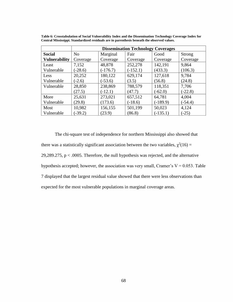
68
Table 6: Crosstabulation of Social Vulnerability Index and the Dissemination Technology Coverage Index for
Central Mississippi. Standardized residuals are in parenthesis beneath the observed values.
The chi-square test of independence for northern Mississippi also showed that
there was a statistically significant association between the two variables, χ2(16) =
29,289.275, p < .0005. Therefore, the null hypothesis was rejected, and the alternative
hypothesis accepted; however, the association was very small, Cramer’s V = 0.053. Table
7 displayed that the largest residual value showed that there were less observations than
expected for the most vulnerable populations in marginal coverage areas.
Dissemination Technology Coverages
Social
Vulnerability
No
Coverage
Marginal
Coverage
Fair
Coverage
Good
Coverage
Strong
Coverage
Least
Vulnerable
7,152
(-28.6)
48,878
(-176.7)
252,278
(-152.1)
142,191
(433.3)
9,864
(106.3)
Less
Vulnerable
20,252
(-2.6)
180,122
(-53.6)
629,174
(3.5)
127,618
(56.8)
9,784
(24.8)
Vulnerable 28,850
(27.5)
238,869
(-12.1)
788,579
(47.7)
118,351
(-62.0)
7,706
(-22.8)
More
Vulnerable
25,631
(29.8)
273,021
(173.6)
657,512
(-18.6)
64,781
(-189.9)
4,004
(-54.4)
Most
Vulnerable
10,982
(-39.2)
156,155
(23.9)
501,199
(86.8)
50,023
(-135.1)
4,124
(-25)

69
Table 7: Crosstabulation of Social Vulnerability Index and the Dissemination Technology Coverage Index for
North Mississippi. Standardized residuals are in parenthesis beneath the observed values.
Dissemination Technology Coverages
Social
Vulnerability
No
Coverage
Marginal
Coverage
Fair
Coverage
Good
Coverage
Strong
Coverage
Least
Vulnerable
6,295
(-4.8)
45,260
(-45.2)
289,972
(0.3)
54,394
(48.9)
1,360
(8.6)
Less
Vulnerable
14,853
(27.4)
113,350
(52.1)
524,336
(-36.6)
81,075
(-12.3)
1,134
(-23.6)
Vulnerable 14,330
(13.3)
129,155
(88.7)
548,882
(-63.0)
86,129
(-12.8)
2,080
(-2.0)
More
Vulnerable
5,376
(-16.0)
300,379
(56.0)
300,379
(56.0)
40,922
(-21.0)
186
(-29.6)
Most
Vulnerable
2,656
(-34.6)
22,138
(-102.9)
232,748
(79.5)
34,287
(4.2)
2,427
(60.1)
There was a statistically significant association between the two variables in
southern Mississippi, χ2(16) = 127,838.690, p < .0005. Cramer’s V was .139, indicating a
small association. Table 8 shows that the largest residuals were found in the marginal
coverage area and good coverage area. In the marginal coverage area, there were fewer
observed occurrences of the less and least vulnerable populations, and more observed
occurrences for the other populations. Conversely, there were more occurrences in good
coverage for the less and least vulnerable and fewer occurrences for the vulnerable
population.

70
Table 8: Crosstabulation of Social Vulnerability Index and Dissemination Technology Coverage Index for
Southern Mississippi. Standardized residuals are in parenthesis beneath the observed values.
Dissemination Technology Coverages
Social
Vulnerability
No
Coverage
Marginal
Coverage
Fair
Coverage
Good
Coverage
Strong
Coverage
Least
Vulnerable
2,606
(-31.6)
14,818
(-148.4)
153,374
(44.0)
36,420
(108.8)
5,910
(85.3)
Less
Vulnerable
8,735
(-26.9)
49,553
(-199.6)
371,071
(80.4)
79,854
(145.8)
5,073
(-3.8)
Vulnerable 12,307
(33.9)
111,389
(130.8)
293,126
(-25.5)
23,481
(-129.2)
1,983
(-44.8)
More
Vulnerable
8,712
(10.6)
92,543
(116.1)
236,415
(-50.2)
26,985
(-68.3)
2,469
(-24.4)
Most
Vulnerable
3,179
(14.3)
39,627
(140.8)
66,788
(-77.6)
4,858
(-71.8)
1,604
(12.3)
Summary The chapter identifies areas of social vulnerability in the state to discover if there
is a correlation between socially vulnerable populations and no to limited dissemination
technology coverage areas. A social vulnerability analysis was developed using 23
demographic and socioeconomic factors to develop a social vulnerability index. The most
prominent social vulnerability factor for the state describes socioeconomic status
(poverty), family structure (female-led households), and race (Black). The most
vulnerable areas of the state are central Mississippi into the Mississippi Delta in the west
and in southwest Mississippi along the Louisiana border.
The knowledge of the locations of socially vulnerable populations allowed for
analysis to be done to observe if there is a relationship between populations and coverage
areas. This study found that there is a small association between socially vulnerable
populations and coverage areas in the different sample areas. In the central and southern

71
parts of the state, it was observed that the less and least vulnerable populations had fewer
observations than expected in marginal coverage areas and more in good coverage areas.
In contrast, the more and most vulnerable populations had more observations than
expected in marginal coverage areas and less in areas of good coverage. These findings
support the hypothesis that socially vulnerable populations are more likely to reside in
areas of limited coverage than other populations.

72
CHAPTER SIX: WARNED TORNADO CASUALTIES
Tornado warnings are issued when a tornado is indicated by radar or sighted by
spotters in Mississippi. Once the tornado warning has been issued, it is intended that
people seek shelter immediately to avoid harm. The number of warning sources an
individual has access, and thus hazard information that they receive, increases the chance
of an adaptive response, so the reduction of sources may affect their reaction to the
warning. Tornado casualty data was observed to determine if there is a relationship
between casualties and lack of dissemination coverage.
Data The tornado data for Mississippi was obtained from the NOAA SPC severe report
database for the time period 1950 through 2015 (Storm Prediction Center, 2016). The
tornado database contains information by state for the time of observation (year, month,
day, time), state, county, F-scale, injuries, fatalities, estimated property loss, estimated
crop loss, beginning and end latitude and longitude, track length (in miles) and width (in
yards), and tornado segment information. Not all data are available for all tornadoes
recorded in the database. Archived NWS tornado warning polygons and NWS Storm
Based Warning Verifications were obtained from the Iowa Environmental Mesonet
(IEM) (IEM, 2016). The tornado warning polygon database includes the issuing WFO,

73
the time that the product was issued and expired, the type of warning, and the area of the
polygon in square kilometers.
Methodology Tornadoes are observed that occurred from 2013 – 2015. The timeframe begins in
2013, because all tornado dissemination technologies were active at that time. (Wireless
Emergency Alerts were not issued until mid-2012.) The tornadoes that resulted in injuries
and/or deaths were extracted from the tornado data, and, if warned, the warning polygons
were extracted for the tornado tracks.
The odds ratio (2 x 2) statistic is utilized to examine the relationship. The odds
ratio is used to measure associations between two dichotomous variables by using a 2 x 2
contingency table. It is common to define the variables as independent and dependent,
even though it is not required. The odds ratio represents the odds that an outcome will
occur given a particular exposure, compared to the odds of the outcome occurring in the
absence of that exposure, defined as
𝑂𝑑𝑑𝑠 𝑟𝑎𝑡𝑖𝑜 = 𝑜𝑑𝑑𝑠 𝑜𝑓 𝑋 𝑖𝑛 𝑒𝑥𝑝𝑜𝑠𝑒𝑑 𝑔𝑟𝑜𝑢𝑝
𝑜𝑑𝑑𝑠 𝑜𝑓 𝑋 𝑖𝑛 𝑢𝑛𝑒𝑥𝑝𝑜𝑠𝑒𝑑 𝑔𝑟𝑜𝑢𝑝.
If the odds ratio is greater than 1, the odds of X in exposed group is greater in the
exposed group, whereas if the odds ratio is less than 1, the odds are less in the exposed
group. An odds ratio of 1 means that the odds are the same (Laerd Statistics, 2016b).

74
In this study, the technology coverage index is defined as the independent
variable and casualties (injuries and/or death) are the dependent variables. To be
dichotomous, the technology coverage index was divided into low and high coverage
with low coverage encompassing no to marginal coverage and high coverage
encompassing fair to strong coverage. The casualties were classified as yes for occurring
along the tornado track and no for occurring in a portion of the tornado warning polygon.
The entire area of the polygon was not used in the analysis, because the no data would
overwhelm the yes data given the area of the warning polygon and the area of the
tornado.
ArcGIS tools are used to prepare the data for analysis. The Buffer tool was used
to place a buffer around the tornado tracks to depict the width of the tornadoes. Another
buffer measuring .75 mile was placed around the tornado track width to represent a
portion of the warned area that was in close proximity to the tornado. The Clip tool was
used on both buffers to extract coverage areas into the desired size to get coverage values.
The Join tool was used to join the casualty data to the tornado track buffer. The tornado
track buffer was joined to the .75-mile buffer, which represents no casualties, using the
Spatial Join tool in order to combine all of the values together: the coverage values and
the casualty values. In SPSS Statistics, an integer value was given to represent the
categories of the nominal values and the statistic was run.
Results There were 31 tornadoes in 2013, 6 of which resulted in 2 deaths and 88 injuries;
in 2014, 11 out of 40 tornadoes resulted in 16 deaths and 209 injuries; in 2015, 2 out of

75
45 tornadoes resulted in 11 deaths and 64 injuries; and, in 2016, 2 out of 46 tornadoes
resulted in 1 death and 2 injuries. All of the tornadoes were warned except for 1 tornado
in 2014 (Figure 14).

76
Figure 14: Tornadoes that caused casualties in 2013 - 2015 with their subsequent warning polygons.
Tornadoes and Warnings
2013 – 2016

77
Table 9 displays the odds ratio results for each of the warned tornadoes that
occurred along with the date of occurrence and number of casualties. Figure 15 through
Figure 18 show where they are located. Thirteen of the 20 tornadoes had odds ratios
greater than 1, indicating that the odds were greater for casualties to occur in low
coverage areas. There were 25 fatalities and 228 injuries attributed to the tornadoes that
occurred in areas with low coverage. The remaining tornadoes had odds ratios less than 1
indicating that those tornadoes occurred in areas where there was high coverage, with one
tornado being solely located in an area with high coverage. Of those tornadoes, two had
odds ratios approximately .01 away from 1, indicating that there could be an almost equal
mixture of high and low coverage areas along the tornado track. The tornadoes that were
warned in areas with high coverage had 5 deaths and 135 injuries; and, of those
casualties, 2 deaths and 60 injuries were located in both low and high coverage areas.
Table 9: The odds ratio results for the odds of low coverage areas resulting in casualties.
Tornado Date Casualty Odds Ratio --
95% Confidence Intervals Injury Fatality
2013
1 2/10/13 - 16:23 3 0 1.970 -- 1.576 – 2.463
2 2/10/13 – 17:03 71 0 0.807 -- 0.451 – 1.446
3 4/11/13 – 10:35 9 1 1.413 -- 1.242 – 1.609
4 12/21/13 – 16:51 2 0 1.656 -- 1.319 – 2.079
5 12/21/13 – 17:19 2 1 1.448 -- 0.931 – 2.251

78
Tornado Date Casualty Odds Ratio --
95% Confidence Intervals Injury Fatality
6 12/21/13 – 17:40 1 0 0.593 -- 0.143 – 2.456
2014
1 4/7/2014 – 1:02 8 0 1.177 -- 0.953 – 1.453
2 4/28/2014 – 13:38 32 0 .988 -- 0.750 – 1.302
3 4/28/14 – 14:51 84 10 1.271 -- 1.077 – 1.500
4 4/28/14 – 15:56 1 0 1.429 -- 0.967 – 2.111
5 4/28/14 – 17:27 10 1 1.339 -- 0.902 – 1.988
6 4/28/14 – 17:38 5 0 2.127 -- 1.095 – 4.131
7 4/28/14 – 18:36 3 0 All in high coverage
8 4/28/14 – 20:40 15 0 1.061 -- 0.764 – 1.474
9 12/23/14 – 14:20 50 3 1.815 -- 1.400 – 2.353
10 12/23/14 – 15:22 0 2 0.361 -- 0.088 – 1.472
2015
1 12/23/15 – 14:54 28 2 0.985 -- 0.826 – 1.175
2 12/23/15 – 16:10 36 9 1.497 -- 1.303 – 1.721
2016
1 02/15/16 – 13:15 2 0 2.300 -- 1.422 – 3.719
2 02/23/16 – 16:15 0 1 0.810 -- 0.614 – 1.068

79
Figure 15: The locations of 2013 tornadoes and warnings on the Dissemination Technology Coverage Index.
2013 Tornadoes and Warnings

80
Figure 16: The locations of 2014 tornadoes and warnings on the Dissemination Technology Coverage Index.
2014 Tornadoes and Warnings

81
Figure 17: The locations of 2015 tornadoes and warnings on the Dissemination Technology Coverage Index.
2015 Tornadoes and Warnings

82
Figure 18: The locations of 2016 tornadoes and warnings on the Technology Dissemination Coverage Index.
2016 Tornadoes and Warnings

83
Summary This chapter incorporated the Dissemination Technology Coverage Index with
past tornado warnings to examine casualties. Warned tornadoes that resulted in injury
and/or death were examined to reveal if there is a correlation between casualties and
coverage areas. The odds ratio was used to calculate the odds of tornado casualties for
warned tornadoes in low coverage areas. The study found that 13 of the 20 warned
tornadoes from 2013 – 2017 occurred in areas of low coverage, resulting in 228 injuries
and 25 fatalities.
The results show that there is a relationship between coverage gaps and tornado-
warned casualties. Although the research supports my hypothesis, it should be noted that
this is a very limited dataset of four years, and a longitudinal study should be performed
to see if the results persist. Additionally, the lack of dissemination coverage may not be
the cause of the casualties. Factors such as the time of tornado occurrence, the person’s
location, whether in a car or a mobile home, along with other factors may have affected
the chances of the injury or fatality.

84
CHAPTER SEVEN: CONCLUSION
This research sought to explore the effectiveness of tornado warning messages by
locating coverage gaps in commonly used dissemination technologies. A Dissemination
Technology Coverage Index was developed using the coverage from reclassified,
aggregated, and weighted digital television, FM radio, and cellular signals, and outdoor
warning sirens. The coverage index categorizes coverage as No Coverage, Marginal
(weak), Fair, Good, and Strong.
The Dissemination Technology Coverage Index was used to test the hypothesis
that socially vulnerable populations are likely to reside in areas with no to marginal
coverage. A social vulnerability index was developed for the state using 23 demographic
and socioeconomic variables. The chi-square test of independence statistic was run for
portions of northern, central, and southern Mississippi to discover if social vulnerability
and coverage areas were independent. For each portion of the state, the chi-square test of
independence showed that there was a statistically significant association between social
vulnerability and coverage areas; however, the Cramer’s V showed that the associations
were small. The association in northern Mississippi was the smallest. To determine
which cells deviated from independence, standardized residuals were examined. In
central Mississippi, there were less observed occurrences than expected in areas of good
coverage for the more and most vulnerable populations, and a higher occurrence of more

85
vulnerable populations in marginal coverage areas. Additionally, in southern Mississippi,
there were higher observations of vulnerable to most vulnerable populations in marginal
coverage areas. In central and southern Mississippi, the higher occurrences of the more
and/or most vulnerable populations in the marginal coverage area supports the
hypothesis.
The Dissemination Technology Coverage Index was also used to test the
hypothesis that casualties from warned tornadoes are more likely to occur where the area
being warned has marginal to no coverage. There were 20 warned tornadoes that
occurred from 2013 – 2016 that resulted in 253 casualties. The odds ratio was used to
calculate the odds of tornado casualties for warned tornadoes in low coverage areas. The
results showed that 13 of the 20 tornadoes occurred in areas with low coverage, and the
other 7 occurred in areas with high coverage. Additionally, the low coverage areas had a
higher number of casualties than those in high coverage areas. This validates the
hypothesis because there is a positive correlation between warned tornadoes with
casualties and areas with low coverage. There are many factors that can contribute to
casualties in severe weather; this study attempts to observe if the lack of dissemination
coverage is one of these factors.
This study is important in that there have been few, if any, warning dissemination
research that examines the availability of warning sources to the public. There has been
research that focused on whether or not a warning was issued, the warning lead times,
and false alarm rates. People have been surveyed on the sources they received
information from, but are less likely to have been asked what sources they have available

86
to them. This research can be used to improve coverage, increase warning dissemination
prior to and during a hazard, and as a research tool. Additionally, the coverage index can
be used by emergency managers, meteorologists, or other hazard scientists, and the
media.
Limitations
This study had some limitations that could have enhanced the research, but did
not adversely affect the results. As previously discussed, one limitation was the extent of
the coverage studied, specifically the cellular coverage. The cellular data use is not the
entire cellular network for the state, since the FCC data does not include cellular towers
that are under 200 feet. Additionally, the cellular coverage was not calculated using the
RF propagation model, because the frequency data for the cellular transmitters was not
readily available. However, the coverages for the cellular towers were represented by the
Cellular Geographic Service Areas, which is a composite of the service areas of all of the
transmitters. Another limitation is that the television coverage is for digital antennas only;
satellite or cable television was not considered in the coverage, so a larger number of
people are getting a television signal that are not being accounted for. Finally, the areas
along the border could be a part of the respective neighboring state’s market and those
transmitters were not included in this dataset.
Second, the social vulnerability index has limiting factors. There are agreed upon
variables that may define one as being socially vulnerable, such as socioeconomic status,
age, race and ethnicity, gender, and disability. In developing the social vulnerability
index for Mississippi, all of the variables that have been used in the development of other

87
vulnerability indexes, such as disability, nursing home occupants, and specific
employment industries, were not used in the development of this index. The inclusion of
those factors in the Principal Component Analysis would not produce an identity matrix,
which shows that the sample data is inadequate for analysis. As previously stated, the
index was based on census tract data, so it generalizes vulnerability factors for a larger
area and does not look at individual communities.
Finally, there were some limitations with the casualties associated with warned
tornadoes. The range of years for examining the casualties for warned tornadoes was
limited due to the time frame in which all four observed technologies were disseminating
warning information. Additionally, assumptions were made when determining the
location of the tornado-related casualties. The storm reports do not list the exact location
of the injury or fatality, so the injuries or fatalities were assumed to have occurred along
the path of the tornado.
Despite these limitations, the research goals were accomplished, and the findings
can be used to enhance warning dissemination.
Applications The Dissemination Technology Coverage Index identifies exposures to
vulnerabilities by displaying gaps in dissemination coverage. The city of Tulsa,
Oklahoma, has demonstrated how research of this kind can be used to improve coverage.
In Tulsa, emergency managers exposed gaps in tornado siren coverage, and are now
seeking to add more sirens so that the entire city would be within the range of a siren

88
(Wade, 2015). Other jurisdictions could use the index in a similar manner to identify gaps
and find ways to fill them.
The National Weather Service has the Weather-Ready Nation initiative whose
purpose is to save more lives by ensuring that the nation is prepared “to protect, mitigate,
respond to and recover from weather-related disasters.” To accomplish this goal, the
NWS is expanding its reach by incorporating new partners, enhancing its operational
initiatives, upgrading radar and satellite technologies, and improving its risk
communication. A specific operational initiative is to increase severe weather warning
lead times and improve how the weather is communicated to the public. The NWS’s
partners, including other government agencies, emergency managers, the private sector,
non-profits, and the media, work to get these weather messages out (NWS, 2011). As the
NWS works to build a Weather Ready Nation, the information gathered from this
research can be utilized. For example, the Dissemination Technology Coverage Index can
be used by Warning Coordination Meteorologists at local weather forecast offices as a
tool to use when hazardous weather will be impacting their county warning area. This
research can act as a reference to where there are areas with limited dissemination
coverage, and allow them to reach out to partners to ensure that the hazard information is
available to more people. Additionally, the social vulnerability index can be used to
locate where the more socially vulnerable populations are, and information, such as
shelter locations and other resources, can be shared with them so that they are aware of
their options for protective actions during hazardous weather. Using both the
Dissemination Technology Coverage Index and a social vulnerability index will provide

89
the NWS with instances of both place and social vulnerability, and allow them to hone in
on areas that are more at risk to hazards.
The coverage index can be a tool used to encourage the utilization of other
information sources. It has been shown that areas with no to limited coverage can play a
factor in casualties and that they may have more socially vulnerable populations. When a
hazard is impending and the affected area is located where there is limited technology
dissemination coverage; emergency managers and/or broadcasters could encourage
family and friends to reach out to those in the threat area, and act as an additional
information source. Additionally, neighborhood associations, local civic organizations,
and/or religious institutions could be made aware of the threat, and they can take action to
ensure that the areas that they serve are aware of the risk and what protective actions to
take, which ties into the NWS Weather Ready Nation initiative.
Future research
There are several ways in which this research can be extended. The research only
examined four dissemination technologies, which was due to two factors: computing
time/power and information availability. The Dissemination Technology Coverage Index
could add more technologies, such as NOAA Weather Radio, broadband internet, and all
of the cellular transmitters. Additionally, the coverage maps are based on mathematical
applications. Field studies could be performed to test the accuracy of the results from the
Free Space Path Loss and sound propagation equations. This will allow the coverage
index to be more accurate.

90
This research does not take into account other factors that that could hinder the
warning messages from reaching the targeted populations, such as power outages. As
previously stated, tornadoes and severe thunderstorms affect transmission and local
distribution (T&D) lines directly through wind damage and indirectly through downed
trees. Partnerships can be developed with the power companies to determine if there are
locational trends for power outages during certain hazards. For example, Dominion
Power in northern Virginia has the capability to know where (according to zip code) there
are outages and how many people are affected. Such locations, if they exist, could be
highlighted in the coverage index as areas with the potential to have decreased
communication. This method can be helpful both proactively and during the event.
Social vulnerability indices can be powerful tools for decision-making in pre-
disaster planning, post-disaster response, and resource allocation. Since it was found that
there is a small relationship between areas with no to limited coverage and socially
vulnerable populations, an index can be developed on a smaller scale to locate vulnerable
populations. For the index to be most effective, it should take into account quantitative
approaches and qualitative approaches. The qualitative approach may be more time
consuming, because it will require communicating with local officials and/or community
members. This method could lead to the development of a social vulnerability index that
will take into account what hazards are more vulnerable to areas, and what specific
variables may make a community vulnerable. If this social vulnerability index were
developed and used in conjunction with the Dissemination Technology Index, emergency
managers and hazard scientists (meteorologists, geologists, etc.) will know where to

91
direct communication to ensure that the populace is getting hazard information, are aware
of available resources, and know what protective actions to take.
The coverage index can be made into an interactive application (app) that covers
the United States and is packaged for hazard scientists and emergency managers to be
used when a hazard is imminent or occurring. The app can allow the respective users to
know where there may be limited messaging before the event, and include a social
vulnerability index. Additionally, if partnerships could be brokered with power
companies, a tool could be added to the app to include active power outages. With this
information, some of the recently stated uses of the Technology Dissemination Coverage
Index can be utilized to inform the at-risk population of the hazard. Regardless of the
approach, it is hoped that hazard warning disseminators could have some influence in
ensuring that all populations receive adequate warning information.

92
REFERENCES
Beede, D. and Neville, A. (2013). Broadband availability beyond the rural/urban divide:
Broadband brief no. 2. Retrieved from
http://www.ntia.doc.gov/files/ntia/publications/broadband_availability_rural_urba
n_june_2011_final.pdf
Brotzge, J. and Donner, W. (2013). The tornado warning process: A review of current
research, challenges, and opportunities. Bulletin of the American Meteorological
Society, 94, 1715 - 1733
Burnside, R., Miller, D.S., and Rivera, J.D. (2007). The impact of information and risk
perception on the hurricane evacuation decision-making of greater New Orleans
residents. Sociological Spectrum: Mid-South Sociological Association, 27, 727 –
740.
Coleman, T.A., Knupp K.R., Spann, J., Elliott, J.B., and Peters, B.E. (2011). The history
(and future) of tornado warning dissemination in the United States. Bulletin of the
American Meteorological Society, 92, 567–82.
Carter-Pokras, O., Zambrana, R.E., Mora, S.E., and Aaby, K.A. (2007). Emergency
preparedness: knowledge and perceptions of Latin American immigrants. Journal of
Health Care for the Poor and Underserved, 18, 465 – 481.
Cutter, S.L., Boruff, B.J., and Shirley W.L. (2003). Social vulnerability to environmental
hazards. Social Science Quarterly, 84, 242 – 261.
Dash, N. and Gladwin, H. (2007). Evacuation decision making and behavioral responses:
Individual and household. Natural Hazards Review, 8, 69 – 77.
Department of Energy. (2013). Economic benefits of increasing electric grid resilience to
weather outages. Retrieved from
http://energy.gov/sites/prod/files/2013/08/f2/Grid%20Resiliency%20Report_FIN
AL.pdf
Demuth, J., Morss, R.E., Morrow, B.H., and Lazo, J.K. (2012). Creation and
communication of hurricane risk information. Bulletin of the American
Meteorological Society, 93, 1133 – 1145.

93
Elliott, J.R., Haney, T.J., and Sams-Abiodun, P. (2010). Limits to social capital:
Comparing network assistance in two New Orleans neighborhoods devastated by
Hurricane Katrina. The Sociological Quarterly, 51, 624 – 648.
ESRI ArcGIS Pro. (2017). Using Viewshed and Observer Points for visibility analysis.
Retrieved from http://pro.arcgis.com/en/pro-app/tool-reference/3d-analyst/using-
viewshed-and-observer-points-for-visibility.htm
Federal Communications Commission. (2012). Federal Communications Commission
Geospatial Data (Data file). Retrieved from
http://wireless.fcc.gov/geographic/index.htm?job=licensing_database_extracts
Federal Communications Commission. (2015). General information about FM and TV
service contour maps and map data. Retrieved from
https://www.fcc.gov/media/radio/general-info-fm-tv-maps-data
Federal Emergency Management Agency. (2006). Outdoor Warning System: Technical
Bulletin (Version 2.0). Retrieved from
http://www.midstatecomm.com/PDF/FEMA_guide.pdf
Federal Signal. (2017). Models 2001-130, Equinox, and 508-128 Sirens: Installation,
Operation, and Service Manual. Retrieved from https://www.fedsig.com.resource-
document/file/9371
Flanagan B.E., Gregory, E.W., Hallisey, E.J., Heitgard, J.L., and Lewis, B. (2011). A
social vulnerability index for disaster management. Journal of Homeland Security
and Emergency Management, 8(1), Article 3.
Fothergill, A., Maestas, E.G.M. and Darlington, J.D. (1999). Race, ethnicity, and
disasters in the United States: A review of the literature. Disasters, 23, 156 – 173.
Hayes, J.L. (2011). NOAA NWS Service Assessment: The Historic Tornadoes of April
2011. Retrieved from
https://www.weather.gov/media/publications/assessments/historic_tornadoes.pdf
Hazards and Vulnerability Research Institute (HVRI). (2013). Social vulnerability index
for the United States – 2006-10. Retrieved from
http://webra.cas.sc.edu/hvri/products/sovi.aspx.
Iowa Environmental Mesonet. (2016). Archived NWS Watch/Warnings (Data file).
Retrieved from https://mesonet.agron.iastate.edu/request/gis/watchwarn.phtml

94
Jewell, V.R. (2014). Use of GIS in readio frequency planning and positioning
applications. Retrieved from
https://vtechworks.lib.vt.edu/bitstream/handle/10919/50499/Jewell_VR_T_2014.p
df?sequence=1
Keifer, J.J., Mancini, J.A., Morrow, B.H., Gladwin, H., and Stewart, T.A. (2008).
Providing access to resilience-enhancing technologies for disadvantaged
communities and vulnerable populations. Oak Ridge, TN: Community and
Regional Resilience Initiative, Oak Ridge National Laboratories.
Laerd Statistics. (2016a). Chi-square test for independence using SPSS Statistics.
Statistical tutorials and software guides. Retrieved from
https://statistics.laerd.com/
______. (2016b). Calculating an odds ration using SPSS Statistics. Statistical tutorials
and software guides. Retrieved from https://statistics.laerd.com/
Laidlaw, E. 2010. The controversy over outdoor warning sirens. Weatherwise 1:16 – 25.
Lane, B. (n.d.). Tech topic 17: Propagation characterization. Retrieved from
http://transition.fcc.gov/pshs/techtopics/techtopics17.html
Lazo, J.K., Morss, R.E., and Demuth, J.L. (2009) 300 billion served: Sources,
perceptions, uses, and Values of Weather Forecasts. Bulletin of the American
Meteorological Society, 90(6), 785 – 798.
Lindell, M.K. and Perry, R.W. (2012). The protective action decision model: The
theoretical modifications and additional evidence. Risk Analysis, 32, 616 – 632.
Lindell, M.K., Prater, C.S., and Peacock, W.G. (2007). Organizational communication
and gecision making for hurricane emergencies. Natural Hazards Review, 8, 50 –
60.
Mazda, F. (Ed.). (1996). Principles of radio communication. Oxford: Focal Press.
Mississippi Automated Resource Information System. (2011). Mississippi Statewide Data
and 2010 Census (Data File). Retrieved from
http://www.maris.state.ms.us/HTM/Data.html
Nagele, D.E. and Trainor, J.E. (2012). Geographic specificity, tornadoes, and protective
action. Weather, Climate, and Society, 4, 145 – 155.

95
National Research Council. (2011). Public response to alerts and warnings on mobile
devices: Summary of a workshop on current knowledge and research gaps.
Washington, D.C., The National Academies Press, pp. 102.
______. (2013). Geotargeted alerts and warnings: Report of a workshop on current
knowledge and research gaps. Washington, D.C., The National Academies Press,
pp.79.
National Weather Service. (2009). Glossary. Retrieved from
http://w1.weather.gov/glossary/
______. (2010). Weather-ready nation: Strategic plan 2011. Retrieved from
http://www.nws.noaa.gov/com/weatherreadynation/files/strategic_plan.pdf
______. (2014). Dissemination Services. Retrieved from
http://www.nws.noaa.gov/os/disemsys.shtml
Nešković, A., Nešković,N., and Paunović, D. (2000). Modern approaches in modeling of
mobile radio systems propagation environment. IEEE Communications Survey.
Received from
http://www.researchgate.net/profile/Natasa_Neskovic/publication/224084444_Mo
dern_approaches_in_modeling_of_mobile_radio_systems_propagation_environm
ent/links/54fcc5d00cf20700c5e96eda.pdf.
Paul, B.K., Stimers, S. and Caldus, M. (2014). Predictors of compliance with tornado
tarnings issued in Joplin, Missouri, in 2011. Disasters, 39, 108 – 124.
Peguero, A.A. (2006). Latino disaster vulnerability: The dissemination of hurricane
mitigation information among Florida’s homeowners. Hispanic Journal of
Behavioral Sciences, 28(5), 5 – 22.
Pender, G. (2017, February 17). 13 things you need to know about the state economy.
The Clarion-Ledger. Retrieved from
http://www.clarionledger.com/story/news/politics/2017/02/16/state-economic-
briefing/97993092/
Perry, R.W. (1979). Evacuation decision making in natural disasters. Mass Emergencies,
4, 25 – 38.
Perry, R.W., Lindell, M.K., and Greene, M.R. (1982). Crisis communication: Ethnic
differentials in interpreting and acting on disaster warnings. Social Behavior and
Personality, 10, 97 – 104.

96
Phillips, B.D. and Morrow, B.H. (2007). Social science research needs: Focus on
vulnerable populations, forecasting, and warnings. Natural Hazards Review, 8, 61
– 68.
Poole, I. (nd). Free space path loss: details, formula, calculator. Radio-Electronics.com.
Retrieved from http://www.radio-electronics.com/info/propagation/path-loss/free-
space-formula-equation.php
Reed, S.E., Boggs, J.L., and Mann, J.P. (2010). SPreAD-GIS: an ArcGIS toolbox for
modeling the propagation of engine noise in a wildland setting. Version 2.0. The
Wilderness Society, San Francisco, CA.
Richards, J.A. (2008). Radio wave propagation: An introduction for the non-specialists.
Berlin: Springer.
Rosu, I. (n.d.). Basics of radio wave propagation. Retrieved from
http://www.qsl.net/va3iul/Antenna/Basics_of_Radio_Wave_Propagation.pdf
Sansing, D.G. (2015). Mississippi. Encyclopedia Britannica. Retrieved from
http://www.britannica.com/EBchecked/topic/385567/Mississippi
Schumacher, R.S., Lindsey, D.T., Schumacher, A.B., Braun, J., Miller, S.D., and Demuth
J.L. (2010). Multidisciplinary analysis of an unusual tornado: Meteorology,
climatology, and the communication an interpretation of warnings. Weather and
Forecasting, 25, 1412 – 1429.
Shaw, J.A. (2013). Radiometry and Friis transmission equation. American Journal of
Physics. 81(33): 33 – 37.
Singer, H. (2013). Is the US losing the broadband race? As it turns out, we look a like
Danica Patrick. Forbes. Retrieved from
http://www.forbes.com/sites/halsinger/2013/02/26/is-the-u-s-losing-the-
broadband-race-as-it-turns-out-we-look-a-lot-like-danica-patrick/
Sizun, H. (2005). Radio wave propagation for telecommunication applications. Berlin:
Springer.
Smith, K.S. and McCarty, C. (2009). Fleeing the storm(s): An examination of evacuation
behavior during Florida’s 2004 hurricane season. Demography, 46, 127 – 145.
Smith, S.W. (1998). The scientist and engineer’s guide to digital signal processing.
Retrieved from http://www.dspguide.com/ch22/1.htm
Spence, P.R., Lachlan, K.A., and Griffin, D.R. (2007). Crisis communication, race, and

97
natural disasters. Journal of Black Studies, 37, 539 – 554.
Stafford, S. (2015). Comparing methods for identifying social vulnerability to
environmental hazards: A case study of coastal Virginia (PDF document).
Retrieved from https://coast.noaa.gov/socialcoast/ppt/Stafford.pdf
Storm Prediction Center. (2015). The online tornado FAQ: Frequently asked questions
about tornadoes. Retrieved from http://www.spc.noaa.gov/faq/tornado/
__________. (2016). Storm Prediction Center SVRGIS (Data file). Retrieved from
http://www.spc.noaa.gov/gis/svrgis/
U.S. Congress, Office of Technology Assessment. (1990). Physical vulnerability of
electric system to natural disasters and sabotage, OTA-E-453. Washington, DC:
U.S. Government Printing Office. Retrieved from
http://ota.fas.org/reports/9034.pdf
U.S. Government Publishing Office (n.d.) Cellular Geographic Service Areas. Retrieved
from https://www.gpo.gov/fdsys/pkg/CFR-2013-title47-vol2/pdf/CFR-2013-
title47-vol2-sec22-911.pdf
Vernier, D. (n.d.) Interference on the FM band. Retrieved from http://www.v-
soft.com/wp-content/uploads/2012/04/Interference_on_the_FM_Band.pdf
Wade, J. (2015, May 15). Covering tornado warning gaps: Tulsa emergency officials
seek funding to add four more sirens. Tulsa World. Retrieved from
http://www.tulsaworld.com/news/local/covering-tornado-warning-gaps-tulsa-
emergency-officials-seek-funding-to/article_42f13d92-42e3-5dfc-8c63-
0b267e2abe63.html
Webster, B. (2014). Emergency siren sound propagation and coverage optimization
analysis (Master’s thesis, University of Redlands). Retrieved from
http://inspire.redlands.edu/gis_gradproj/223

98
BIOGRAPHY
Aisha C. Reed Haynes graduated with an International Baccalaureate Diploma from Jim
Hill High School, Jackson, MS in 1998. She received her Bachelor of Science from
Jackson State University in 2002, and her Master of Science from Purdue University in
2006.