An Investigation of Event Study Methodologies with Clustered Events and Event Day Uncertainty

JOBNAME: Kluwer Journals − GR PAGE: 1 SESS: 20 OUTPUT: Tue May 27 14:37:15 1997/data11/kluwer/journals/requ/v8n3art2

Review of Quantitative Finance and Accounting, 8 (1997): 211–228© 1997 Kluwer Academic Publishers, Boston. Manufactured in The Netherlands.

An Investigation of Event Study Methodologies withClustered Events and Event Day Uncertainty

SANG H. LEEDirector, International Securities Division, and Research Fellow, The Korea Securities Research Institute,(The Korea Securities Dealers Association), 34 Yeoeuido-Dong, Youngdeungpo-GU, Seoul 150-010, Korea

OSCAR VARELAProfessor of Finance, Department of Economics and Finance, University of New Orleans, New Orleans, LAUSA 70148

Abstract. The specification and power of mean-adjusted, market and quadratic models in event studies usingOLS, Patell, Jaffe and GLS are examined. Simulation is used with security and portfolio returns to capturedifferent cross correlations. The market model is always superior in specification and power compared to themean-adjusted and quadratic models. The use of OLS with the market model is supported in the absence ofclustered events and event day uncertainty, whereas use of Jaffe with the market model is supported in thepresence of these problems.

Key words: Event Study Methods, Contemporaneous Correlations, Event Clustering, Event Day Uncertainty

Empirical investigations concerning the efficiency of financial markets often examine theeffect of a particular event on a firm’s stock returns. One persistent question concerningevent studies is the use of appropriate models and test methods for different circum-stances, one of which involves clustered events and event day uncertainty. Theoreticaldiscussions point toward the use of generalized least squares (GLS) in event studies of thistype.

The cumulation of returns and clustering of events in calendar time conceptually jus-tifies use of GLS, since contemporaneous correlations of returns are produced by overlapsbetween different firm’s event windows.1 However, given the existence of alternative andless cumbersome test procedures, an outstanding issue when clustered events and eventday uncertainty exist is the specification and power of GLS compared to alternative testprocedures.2

This study addresses this question by simulating experiments across firms and portfo-lios. The motivation for experimenting across both firms and portfolios is to capturediffering levels of cross correlations in returns. Various methodologies, including OLS,Patell (1976), Jaffe (1974) and GLS, are examined.

Tests for significant differences between actual and required returns are based oncumulative abnormal returns (CAR). This approach is appropriate in listing studies,among others, in which the calendar date of the event impact cannot be accurately pin-

Kluwer Journal@ats-ss3/data11/kluwer/journals/requ/v8n3art2 COMPOSED: 05/05/97 3:07 pm. PG.POS. 1 SESSION: 19

5% 50% 90% 100%


pointed. For example, even though the Wall Street Journal or Financial Times may an-nounce a stock listing or a change in regulatory policy on a specific date, prior release orleakage of information is possible. In these cases, expectations regarding the announce-ment create uncertainty as to the exact event date. In general, the potential for event datemisspecification arises whenever price data are reported more precisely than informationabout the event date.

The paper proceeds as follows. Section 1 presents a literature review while Section 2discusses the sample and data. Section 3 discusses the methodology while Section 4presents the results. Section 5 summarizes the study and presents conclusions.

1. Literature review

Prior studies have shown that cross correlations from event time clusterings are not aproblem for abnormal returns on a non-cumulative basis (AR) as long as the sampledfirms are diversified and the market model is used. However, the seriousness of testingbiases will likely be higher when returns are cumulated over a long event window. Un-fortunately, prior studies provide little guidance regarding the advantages of GLS whenreturns are cumulated over lengthy event windows.

Fama, Fischer, Jensen and Roll (1969) were the first to employ the CAR methodology.Schipper and Thompson (1983) suggest advantages from utilizing cross-sectional depen-dency in a joint GLS framework based on Zellner’s seemingly unrelated regressionmethod. Collins and Dent (1984) propose a GLS method to estimate the mean effect ofabnormal performance when there exists potential cross-sectional dependency in returnsdue to clustered event time. Brown and Warner (1985) simulated abnormal returns usingactual return data for randomly selected samples, and found that the market model wasrobust in the presence of cross correlations. However, the power of these tests decreasedsubstantialy with cumulated returns, suggesting that cross correlation problems may beaggravated in the CAR framework with clustered event time.3

Malatesta (1986) confirmed Brown and Warner’s conclusions, and noted that the po-tential benefits of using GLS in event studies are theoretically greater when disturbanceterms are highly correlated across equations such as in industry specific studies. However,Malatesta (1986) and later McDonald (1987) found that little is gained from a system ofequations approach. Bernard (1987) shows that the bias due to cross sectional dependen-cies can be a serious matter regardless of how well diversified the sample is, and con-cludes that a GLS approach might be useful when sufficient time series data exist. Chan-dra, Moriarity and Willinger (1990) reexamined the power of various models, and showthat there is no advantage to using tests which ignore cross-sectional dependencies.

Chandra and Balachandran (1992) provide alternative ways to model GLS, and find thattheir portfolio least squares and constant correlation models have better small sampleproperties than GLS. However, they do not examine conditions involving cumulatedreturns and/or event day uncertainty. In contrast, Ball and Tourous (1988) provide amaximum-likelihood method to examine security price performance with the mean-adjusted return model in a CAR framework given event date uncertainty, and find that

212 SANG H. LEE AND OSCAR VARELA


5% 50% 90% 100%


their method is more efficient than traditional event-study methods. However, their studyassumes independence of events across firms, and hence does not consider the problem ofclustering of event dates and contemporaneous correlations of returns.

Boehmer, Musumeci and Poulsen (1991) examine the problems associated with event-induced variance conditions. They develop a standardized cross sectional test by modi-fying Patell’s (1976) method of weighted least squares and found it to be better specifiedwith higher power than alternative test procedures when event-induced variance changesoccur. Corrado (1989) developed a non-parametric test for event studies and found that therank test statistic was better specified and more powerful than parametric t-tests, androbust against conditions of event-induced variance increases. Corrado (1993) furtherdeveloped a boundary crossing test procedure to eliminate biases stemming from eventperiod uncertainty. While addressing specific and relevant issues in event studies, Boeh-mer, Musumeci and Poulsen (1991) and Corrado (1989 and 1993) do not address theproblem associated with event day clustering and cross sectional dependence.

Campbell and Wasley (1993) found that Corrado’s rank test statistic was better speci-fied with higher power, compared to portfolio and standardized parametric test statisticsfor event studies using NASDAQ returns (in which distributional properties are clearlynon-normal). This study, although considering the problem of event day clustering, doesnot examine this issue within a GLS framework.

Strong (1992), in a review article, concludes that when event day clustering is a prob-lem some correction should be made for cross sectional dependence. Judge, Hill, Grif-fiths, Lutkepohl and Lee (1988, p. 341–342) also show that interval estimates and hy-potheses tests should be based on GLS rather than OLS when cross sectional dependenceexists. This point is supported by Boehmer, Musumeci and Poulsen (1991), although theysuggest that “data limitations and difficulty of implementation” (p. 255) have causedresearchers to generally ignore the use of GLS. This paper aims to fill this void from apractical point of view by examining whether correction for cross sectional dependenceimproves the performance of test procedures sufficiently to justify its use.

2. Sample and data

Security returns were extracted at random from the CRSP NYSE/AMEX daily return filesfor the two year period (including 505 observations) from January 2, 1985 to December31, 1986. This two year period provides a data set sufficiently short to simulate event dataclustering. The market index used is the equally weighted CRSP index. The event windowis 11 days long, including 5 days before and after the event (25,…,0,…15). Eachwindow is randomly chosen from between the 260th and 490th trading days in the twoyear period. The window is fixed for each simulation trial (defined below), although thewindow differs randomly between trials.

The hypothetical event day, i.e. day 0, for each trial is the sixth day in the 11 day(25,…,0,…15) event window. The actual event day for each of the 50 firms or portfoliosin a trial differs randomly within the 11 day window. Thus, actual event days are bothclustered and uncertain. A total of 261 daily observations were collected around each

AN INVESTIGATION OF EVENT STUDY METHODOLOGIES 213


5% 50% 90% 100%


hypothetical event day. The hypothetical event day is the 256th day within the set of 261daily observations collected for each firm. Abnormal returns, of course, are imposed onthe random actual event days.

The estimation period from which model parameters are obtained is the first 240observations per trial; 10 observations were omitted between the end of the estimationperiod and beginning of the test period. An 11 day test period is used, including 5 daysbefore and after the hypothetical event day as well as the hypothetical event day itself.

The experiments include samples of ten, twenty-five and fifty firms (securities) per trial,and fifty portfolios per trial each composed from the equally weighted return distributionsof both five and ten randomly selected firms (securities). In experiments with individualsecurities and with portfolios of five securities, trials are simulated 250 times. In experi-ments with equally weighted portfolios of ten securities, trials are simulated 100 times dueto the larger number of firms included in these simulations. As such, even though theportfolios may seem rather small, especially for the five firm case, the calculation of eachtrial’s abnormal return is based on an average of 250 firms for the five firm portfolios (5firms times 50 portfolios per trial) and 500 firms for the ten firm portfolios (10 firms times50 portfolios per trial). Finally, samples for each trial are drawn without replacement.

The random nature of samples and event periods provides an initial set of returndistributions upon which abnormalities of from 1 to 5 percent are introduced on the actualevent day during the event window. The specification and power test results across models,tests methods and return abnormalities are based on the 250 simulated trials for firms andportfolios of five firms, and 100 simulated trials for portfolios of ten firms.

3. Methodology

The statistical tests utilize the Collins and Dent (1984) GLS procedure modified to ac-count for the cross-correlation problems in a cumulated return (CAR) framework. Testprocedures also include OLS, as well as Patell (1976) and Jaffe (1974) methodologies.The Patell approach is essentially equivalent to estimating CAR via weighted least squaresrather than OLS. The Jaffe approach forms a portfolio of sample securities in calendartime and attempts to account for cross correlations by measuring the residual variancedirectly from the portfolio.

3.1. The general model

Let ri,t designate the observed return for security i at day t. For every security, theabnormal return for each day t in the test period, denoted ei,t, is given by

ei,t 5 ri,t 2 E~ri,t!, (1)



5% 50% 90% 100%


where i 5 1,2,…, N (firm index); t 5 T1 (starting day) to T2 (ending day) of the testperiod, such that T1 could be some days before the event on day 0; E(ri,t), is the ex-anteexpected return for firm i at time t; and ei,t is the measure of abnormal performance forfirm i at time t in the test period.

The expected return for firm i, E(ri,t), is obtained from the general linear return gen-erating model using T observations in the estimation period,

ri 5 X • bi 1 ei, (2)

where X is a known (T 3 K) nonstochastic design matrix of rank K with the first columnbeing 1s; b is a K-dimensional fixed vector of unknown parameters; and ei, the residualfrom the return generating model in the estimation period, is a (T 3 1) vector of anunobservable random variable in the estimation period with mean zero and identically andindependently distributed errors.

Three forms corresponding to different return generating processes of the design matrixX were initially considered in this study. The mean-adjusted model, however, was poorlyspecificied in all simulations, and the market model was superior in specification andpower relative to the quadratic. As such, the methodology and results presented below arejust for the market model, in which case the design matrix X has vectors of 1s and marketreturns.4 In non-matrix form, this model is shown as

ri 5 ai 1 birm 1 ei, (3)

where ai is the intercept and bi the coefficient for the market return variable.5

3.2. Estimation of abnormal returns in GLS

The measure of abnormal performance during the testing period, ei,t, as shown in (1) maybe cross sectionally correlated when the event time for each firm is contemporaneous orclustered within a narrow window of calendar time. Therefore, the cross sectional mean ofabnormal performances at each day t in the test period can be estimated with the followingregression (in matrix format after suppressing the firm index i),

jt 5 ARt • 1 1 nt, nt ; N~0, St!, (4)

where jt8 5 [e1,t, e2,t, …,eN,t]; ARt is both the mean of a vector of N residuals at time t,i.e. the mean of ei,t (i 5 1 to N), and an estimator of the cross-sectional mean abnormalperformance; 1 is a column vector of 1s; and nt is an N-dimensional vector of error terms,distributed with mean zero and variance-covariance matrix St.

The event has no economic effect if the coefficient ARt in (4) is equal to zero. Theproperty of the variance-covariance structure in St dictates an appropriate estimationprocedure. This procedure follows Collins and Dent (1984) as shown in Appendix A, suchthat the appropriate test statistic to examine the null hypothesis that ARt equals zero is,



5% 50% 90% 100%


ARt • @18Vt211#0.5/ft, (5)

where ARt is equal to @18Vt211#2118Vt

21jt, Vt is a consistent estimator of CtVCt, Ct

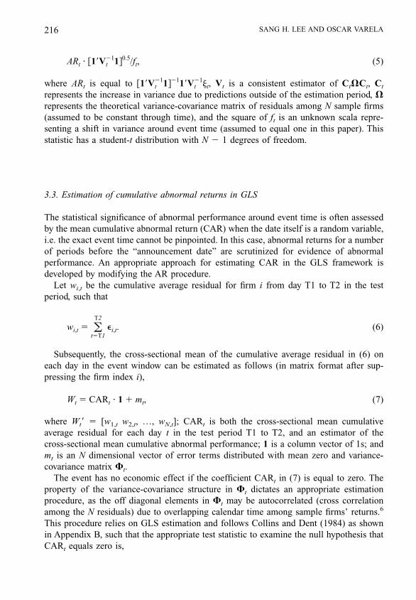
represents the increase in variance due to predictions outside of the estimation period, Vrepresents the theoretical variance-covariance matrix of residuals among N sample firms(assumed to be constant through time), and the square of ft is an unknown scala repre-senting a shift in variance around event time (assumed to equal one in this paper). Thisstatistic has a student-t distribution with N 2 1 degrees of freedom.

3.3. Estimation of cumulative abnormal returns in GLS

The statistical significance of abnormal performance around event time is often assessedby the mean cumulative abnormal return (CAR) when the date itself is a random variable,i.e. the exact event time cannot be pinpointed. In this case, abnormal returns for a numberof periods before the “announcement date” are scrutinized for evidence of abnormalperformance. An appropriate approach for estimating CAR in the GLS framework isdeveloped by modifying the AR procedure.

Let wi,t be the cumulative average residual for firm i from day T1 to T2 in the testperiod, such that

wi,t 5 (t5T1

T2

ei,t. (6)

Subsequently, the cross-sectional mean of the cumulative average residual in (6) oneach day in the event window can be estimated as follows (in matrix format after sup-pressing the firm index i),

Wt 5 CARt • 1 1 mt, (7)

where Wt8 5 [w1,t w2,t, …, wN,t]; CARt is both the cross-sectional mean cumulativeaverage residual for each day t in the test period T1 to T2, and an estimator of thecross-sectional mean cumulative abnormal performance; 1 is a column vector of 1s; andmt is an N dimensional vector of error terms distributed with mean zero and variance-covariance matrix Ft.

The event has no economic effect if the coefficient CARt in (7) is equal to zero. Theproperty of the variance-covariance structure in Ft dictates an appropriate estimationprocedure, as the off diagonal elements in Ft may be autocorrelated (cross correlationamong the N residuals) due to overlapping calendar time among sample firms’ returns.6

This procedure relies on GLS estimation and follows Collins and Dent (1984) as shownin Appendix B, such that the appropriate test statistic to examine the null hypothesis thatCARt equals zero is,



5% 50% 90% 100%


CARt/@18Ft211#20.5, (8)

which has a student-t distribution with N 2 1 degrees of freedom.

3.4. Estimations of cumulative abnormal returns in OLS, Patell and Jaffe testprocedures

OLS estimations of CAR and its variance, given the framework in equations (1) and (6)and assuming independent and identically distributed disturbances among sample firms’returns, are7

CARt 5 ~1/N! • (i51

N

wi,t, and (9)

var~CARt! 5 st2/N (10)

where st2 5 ~1/~N 2 1!! • (i51

N ~wi,t 2 CARt!2.

The appropriate test statistic to examine the null hypothesis of no cumulative abnormalreturns is (9) divided by the square root of (10), which has a student-t distribution with N2 1 degrees of freedom.

Patell (1976) estimation standardizes, similar to the experiments in Brown and Warner(1980, n46), the cumulative abnormal performances for each firm, wi,t by their standarddeviations, such that

CARt ~Standardized! 5 ~1/N! • (i51

N

~wi,t/fi,t! (11)

where fi,t is obtained from (B.2) in Appendix B. This approach is essentially equivalentto estimating CARt via weighted least squares and offers distinct advantages over theconventional OLS test which gives equal weight to all observations. The Patell t-teststatistic is given by,

CARt ~Standardized!/~N0.5!. (12)

These two test methods—OLS and Patell—do not consider the problem of cross-sectional dependence in CAR. In contrast, a time-series of average excess returns from aportfolio of all sample firms, as employed by Jaffe (1974) and Mandelker (1974), providesone way to account for cross-sectional dependence between the residuals of differentfirms.



5% 50% 90% 100%


In this method, measurement of the residual variance directly from the portfolio ac-counts for the cross-sectional dependence in a given calendar time. The residuals fordifferent calendar times are then standardized by their standard deviation as calculatedfrom a block of portfolio residuals around the event time in question.

Jaffe’s approach to estimate the variance of the portfolio residuals reduces to,8

var~ARt! 5 ~181!2118Vt 1~181!21, (13)

and the variance of CARt can be specified as,

var~CARt! 5 ~181!2118Ft 1~181!21, (14)

both of which are greater than the GLS estimates [shown in Appendix A and B as (A.6)and (B.5)], unless the variance of forecast errors are equal across all securities. The Jaffetest statistic to examine the null hypothesis of no cumulative abnormal returns is theestimate of CARt shown in Appendix B as (B.1) divided by the square root of (14), whichhas a student t-distribution with N 2 1 degrees of freedom.

4. Results

Table 1 shows the specification and power test results for the simulations using ten,twenty-five and fifty randomly selected securities per trial. Table 2 shows similar resultsfor the simulations using fifty randomly selected portfolios per trial, with each portfolioconsisting of both five and ten randomly selected securities.

The results in these tables are specifically for the market model with OLS, Patell, Jaffeand GLS given one and five percent significance levels, and simulated mean abnormalreturns of zero, one, two and five percent. The specification of the test methods is exam-ined by evaluating the rejection rates (or incidence of type I errors) pertaining to a meancumulative abnormal return of zero percent. The power is examined by evaluating thefrequency of rejection rates when positive abnormal returns exist. Throughout, the ma-jority of the security and portfolio estimated market models’ beta parameters are signifi-cant.9

4.1. Results for individual security simulations

Table 1 shows that the market model with OLS, regardless of the number of individualsecurities in the simulations or level of significance, is the best specified procedure. Allrejection rates with OLS are within the 95 percent upper confidence limits of 2.04 and7.27 percent for the one and five percent significance levels, respectively.10 Jaffe’s rejec-tion rates, although higher than OLS, are also within the 95 percent upper confidencelimits, except for the ten security simulations at the one percent significance level. In this



5% 50% 90% 100%


case, the rejection rate is within the 99 percent upper confidence limit of 2.47 percent. Theresults are somewhat weaker for Patell, although its rejection rates are most often withinacceptable confidence limits (except for the twenty-five security simulations at the fivepercent significance level).

GLS is the poorest specified procedure in the individual security simulations, failingmost often to show rejection rates within acceptable limits. GLS also has a size problemas its rejection rates at zero percent abnormal return are about twice as high compared tomost other tests regardless of level of significance. The apparent high power of GLS istherefore ignored in further comparisons owing to its misspecifications in the individualsecurity simulations. Instead, Patell produces the highest power with acceptable specifi-cations regardless of the significance level, except as previously noted. Comparisons of

Table 1. Specification and power test results for abnormal return simulations based on the market model acrossindividual securities for various t-test procedures.

SIGNIFICANCE LEVEL

One Percent Five Percent

Spf/1Test

PowerTests

Spf/1Test

PowerTests

ABNORMAL RETURN .00 .01 .02 .05 .00 .01 .02 .05

OLS T-TESTTen Securities .008a .032 .068 .43 .048a .1 .4 .68Twenty-five .008a .039 .15 .80 .048a .15 .36 .92Fifty .000a .048 .264 .936 .040a .212 .548 .984PATELL T-TESTTen Securities .012a .043 .12 .54 .056a .16 .29 .78Twenty-five .024b .13 .24 .93 .092 .23 .44 .97Fifty .024b .116 .428 .992 .072a .280 .612 .992JAFFE T-TESTTen Securities .024b .032 .079 .37 .064a .1 .2 .64Twenty-five .012a .052 .14 .72 .056a .15 .30 .92Fifty .000a .048 .224 .960 .036a .180 .488 .980GLS T-TESTTen Securities .024b .048 .15 .58 .071a .2 .31 .8Twenty-five .043 .13 .30 .91 .10 .23 .46 .98Fifty .040 .212 .496 .992 .092 .352 .680 .992

NOTE: The results shown pertain to the proportion out of 250 trials where the null hypothesis that the meancumulative abnormal returns (CAR) for the interval (25, 15) is equal to zero was rejected against the alternativethat CAR is not equal to zero using daily data and portfolios of 10, 25 and 50 randomly selected securities’returns per trial. For each trial abnormal performance is introduced for one day in the interval (25, 15) witheach day having an equal probability for selection. The symbols “a” and “b” indicate that the specification tests’rejection rates are less than the upper values of the respective 95 and 99 percent confidence intervals as shownbelow.1/ Spf refers to the specification test. The upper value of the 99 percent confidence interval for one percentsignificance is 2.47 percent and for five percent significance 8.21 percent. The upper value of the 95 percentconfidence interval for one percent significance is 2.04 percent and for five percent significance 7.27 percent.(Calculations are shown in endnote 10 and all lower values are zero percent.)



5% 50% 90% 100%


OLS and Jaffe show that OLS generally has higher power, especially at five percentsignificance. The results are best with fifty securities in each simulated trial instead oftwenty-five or ten.

In summary, the best specified test procedure in the individual security simulationsacross securities and significance levels is OLS, although Jaffe also exhibits good speci-fications. Other procedures are not as well specified, and OLS generally has higher powerthan Jaffe. Hence, investigations for abnormal returns when clustered events and event dayuncertainty are not a problem lean toward the familiar use of OLS and the market model.

Table 2. Specification and power test results for abnormal return simulations based on the market model acrossportfolios of five and ten randomly selected securities for various t-test procedures.

SIGNIFICANCE LEVEL

One Percent Five Percent

Spf/1Test

PowerTests

Spf/1Test

PowerTests

ABNORMAL RETURNS .00 .01 .02 .05 .00 .01 .02 .05

OLS T-TEST5 firm portfolio .020a .420 .864 1.0 .100 .584 .956 1.010 firm portfolio .09 .99 1.0 1.0 .14 1.0 1.0 1.0PATELL T-TEST5 firm portfolio .028 .440 .912 1.0 .100 .600 .972 1.010 firm portfolio .10 .99 1.0 1.0 .13 1.0 1.0 1.0JAFFE T-TEST5 firm portfolio .012a .260 .836 1.0 .060a .536 .932 1.010 firm portfolio .03b .99 1.0 1.0 .09b 1.0 1.0 1.0GLS T-TEST5 firm portfolio .024b .440 .884 1.0 .100 .616 .952 1.010 firm portfolio .05 1.0 1.0 1.0 .16 1.0 1.0 1.0

NOTE: The results shown pertain to the proportion out of 250 trials for the five firm portfolios and out of 100trials for the ten firm portfolios where the null hypothesis that the mean cumulative abnormal returns (CAR) forthe interval (25, 15) is equal to zero was rejected against the alternative that CAR is not equal to zero.Portfolios of fifty randomly selected portfolios’ returns per trial were used. Each of the 50 portfolio’s returns arebased on an equally weighted average of both 5 and 10 randomly selected securities’ returns, and for each trialabnormal performance is introduced for one day in the interval (25, 15) with each day having an equalprobability for selection. The symbols “a” and “b” indicate that the specification tests’ rejection rates are lessthan the upper values of the respective 95 and 99 percent confidence intervals as shown below.1/ Spf refers to the specification test. The computed confidence intervals for the simulations with 5 firmportfolios involving 250 trials are shown in Table 1. The computed confidence intervals for the simulations with10 firm portfolios involving 100 trials are as follows. The upper value of the 99 percent confidence interval forone percent significance is 3.32 percent and for five percent significance is 10.08 percent. The upper value of the95 percent confidence interval for one percent significance is 2.64 percent and for five percent significance is8.59 percent. (Calculations are shown in endnote 10 and all lower values are zero percent.)



5% 50% 90% 100%


4.2. Results for portfolio simulations

Table 2 shows the results for the five and ten firm portfolio simulations which, as previ-ously mentioned, introduce into the return stream higher cross correlations based on therationale that the level of correlation of returns for portfolios of randomly selected secu-rites is higher than that for randomly selected securites.11

This table shows that the market model for the five and ten firm portfolio simulationsis well specified with Jaffe regardless of significance level. In these cases, rejection ratesare within the relevant upper value of the 95 percent confidence limits for the five firmportfolio simulations and the 99 percent confidence limits for the ten firm portfoliosimulations. The only other tests that are well specified with the market model are OLSand GLS at the one percent significance level with five firm portfolios. The former’srejection rate is within the upper value of the 95 percent confidence limit and the latter’swithin the upper value of the 99 percent confidence limit (one percent significance). Noneof the other tests, including all involving Patell, are well specified.

In summary, the only test procedure for the portfolio simulations that is well specifiedacross portfolios and significance levels is Jaffe. Other test procedures are problematicalgiven their generally poor specifications, and therefore their higher power is ignored infurther comparisons. Hence, investigations for abnormal returns with clustered events andevent day uncertainty lean toward use of Jaffe and the market model. It is noteworthy thatthis method, unlike OLS and Patell, considers the cross sectional dependency problem inCAR.

4.3. Results for regression analysis

Table 3 shows the results of the regression analysis of the five firm portfolio experiments’rejection rate t-values and mean correlation coefficients of the sample portfolio’s residu-als, with the latter serving as the independent variable. The simple OLS regression isshown below, such that

T-valuek 5 a 1 b ~mean rk! (15)

where T-valuek is the rejection rate t value for trial k (k 5 1 to 250) and (mean rk) is themean correlation coefficient of the sample portfolio’s residuals for trial k (k 5 1 to 250).

The purpose of this regression is to examine the sensitivity of the test methods to thedegree of cross correlation in the residuals of the five firm portfolio experiments. Resultsare not presented for the ten firm portfolio experiments owing to the strength of the resultsfor the five firm portfolios. The regression coefficient b is expected to be significantlynegative when abnormal returns are positive, as a high correlation coefficient in theresiduals require a larger adjustment in the estimated variance of the residuals and hence



5% 50% 90% 100%


produce lower t-values in the hypothesis test. However, when no abnormal returns exist,a zero t-value is theoretically expected so that any adjustment for cross correlation shouldhave no effect on the rejection rate.

The negative regression coefficients in Table 3 are most often significant only whenabnormal returns are positive and the test methods involve either Jaffe or GLS. Theseresults are consistent with expectations as both methods are geared to account for crosscorrelations in the residuals and show no significant coefficient when abnormal returnsequal zero. By comparison, the OLS and Patell test procedures produce no significantregression coefficients. Overall, these results reinforce the conclusions in Section 4.2concerning the Jaffe procedure.

5. Summary and conclusions

In many event studies, sample firms’ reactions to a given event may be clustered in eventor calendar time and the exact time of the event impact may itself be unknown. In thesecircumstances, CAR’s are often used to assess any abnormal effects of the event impacton the stock price. This approach, however, presents potential problems of cross correla-tion in the residuals of sample firms even when event and calendar times are not identical.

This paper examines the specification and power of alternative procedures for identi-fying abnormal returns. In particular, this study compares using a simulation approachwith both individual securities and portfolios the specification and power of OLS, Patell,Jaffe, and GLS using the mean-adjusted, market, and quadratic return generating models.The purpose of using both individual securities and portfolios is to introduce with thelatter higher cross correlations of returns. Overall, the mean-adjusted model was poorly

Table 3. Coefficients of regressions of five firm portfolio experiments rejection rate t-values against the meancorrelation coefficients of sample portfolios’ residuals for the market model with various t-test procedures andabnormal returns.

ABNORMAL RETURNS 0.00 0.01 0.02 0.05

OLS T-TEST 234.93* 224.44 213.96 217.46(21.70) (21.15) (20.60) (20.51)

PATELL T-TEST 226.23 226.56 226.89 227.89(21.14) (21.62) (21.18) (21.20)

JAFFE T-TEST 220.60 242.97** 265.34*** 2132.40***(21.17) (22.45) (23.67) (26.74)

GLS T-TEST 25.62 240.78* 275.93*** 2181.40***(20.24) (21.75) (23.26) (27.53)

NOTE: Results are not presented for the ten firm portfolios owing to the strength of the results for the five firmportfolios. The numbers in the parentheses represent t-statistics for the estimated coefficients. One percent levelof significance is denoted by ***, five percent by ** and ten percent by *. These OLS coefficients are expectedto be significantly negative when abnormal returns are positive (and zero otherwise) if the model captures highcross correlations of returns.



5% 50% 90% 100%


specified in all simulations, and the market model was superior in specification and powerrelative to the quadratic. The recommendations suggested by the results, therefore, arebased on use of the market model.

The best specified test procedure in the individual security simulations across securitiesand significance levels is OLS. Other procedures are not as well specified, although Jaffealso has good specifications. However, comparisons between OLS and Jaffe show thatgenerally OLS has higher power. As such, investigations for abnormal returns whenclustered events and event day uncertainty are not a problem support the familiar use ofOLS and the market model. In contrast, the only test procedure for the portfolio simula-tions that is well specified across portfolios and significance levels is Jaffe. As such,investigations for abnormal returns with clustered events and event day uncertainty sup-port the use of Jaffe and the market model. It is noteworthy that Jaffe, unlike OLS andPatell, considers the cross sectional dependency problem in CAR, and that the theoreticaldiscussions pointing toward use of GLS are not supported in the simulations owing topoor specifications.

Appendix A: GLS test statistic for abnormal returns

Following Collins and Dent (1984), the variance-covariance matrix St is expressed ingeneral form as,

St 5 CtVCt ft2, (A.1)

where Ct reflects the increase in variance due to predictions outside of the estimationperiod T,12 V represents the theoretical N 3 N variance-covariance matrix of residualsamong N sample firms (assumed to be constant through time), and ft

2 is an unknown scalarepresenting a shift in variance around event time.

The Ct is a diagonal matrix of dimension N 3 N with the specific element for firm igiven by,

Ci,t 5 =1 1 Xt~X8X!21Xt8, (A.2)

where Xt is a row vector of the realized value for regressor X in (2) at time t.The elements in V are specified by si,j, and consistently estimated as,

si,j 5 ~1/T 2 K! • (t51

T

~ei,t • ej,t!, (A.3)

where t equal to one identifies the beginning of the estimation period and T the end of theestimation period.



5% 50% 90% 100%


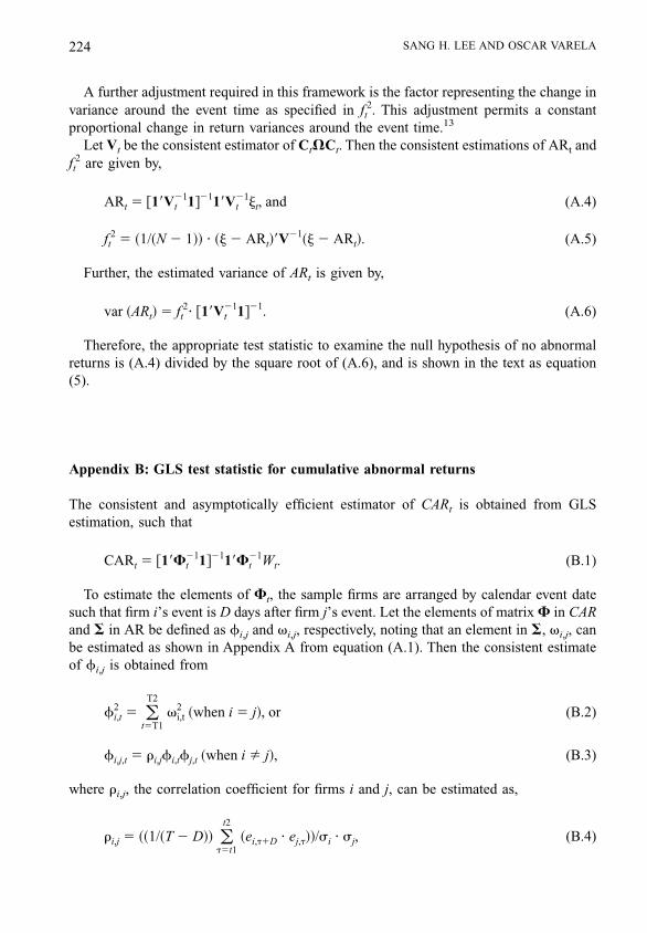
A further adjustment required in this framework is the factor representing the change invariance around the event time as specified in ft

2. This adjustment permits a constantproportional change in return variances around the event time.13

Let Vt be the consistent estimator of CtVCt. Then the consistent estimations of ARt andft

2 are given by,

ARt 5 @18Vt211#2118Vt

21jt, and (A.4)

ft2 5 ~1/~N 2 1!! • ~j 2 ARt!8V

21~j 2 ARt!. (A.5)

Further, the estimated variance of ARt is given by,

var ~ARt! 5 ft2• @18Vt

211#21. (A.6)

Therefore, the appropriate test statistic to examine the null hypothesis of no abnormalreturns is (A.4) divided by the square root of (A.6), and is shown in the text as equation(5).

Appendix B: GLS test statistic for cumulative abnormal returns

The consistent and asymptotically efficient estimator of CARt is obtained from GLSestimation, such that

CARt 5 @18Ft211#2118Ft

21Wt. (B.1)

To estimate the elements of Ft, the sample firms are arranged by calendar event datesuch that firm i’s event is D days after firm j’s event. Let the elements of matrix F in CARand S in AR be defined as fi,j and vi,j, respectively, noting that an element in S, vi,j, canbe estimated as shown in Appendix A from equation (A.1). Then the consistent estimateof fi,j is obtained from

fi,t2 5 (

t5T1

T2

vi,t2 ~when i 5 j!, or (B.2)

fi,j,t 5 ri,jfi,tfj,t ~when i Þ j!, (B.3)

where ri,j, the correlation coefficient for firms i and j, can be estimated as,

ri,j 5 ~~1/~T 2 D!! (t5t1

t2

~ei,t1D • ej,t!!/si • sj, (B.4)



5% 50% 90% 100%


with t1 representing commencement and t2 termination of the estimation period, and si

and sj obtained from the square root of equation (A.3) in Appendix A (when i 5 j for alli’s and all j’s, respectively).

Further, the estimated variance of CARt is given by,

var~CARt! 5 @18Ft211#21. (B.5)

Therefore, the appropriate test statistic to examine the null hypothesis of no cumulativeabnormal returns is (B.1) divided by the square root of (B.5), and is shown in the text asequation (8).

Acknowledgement

The authors thank the Journal’s two anonymous referees for their many comments whichsubstantively improved the quality of this paper. The usual caveat applies as the authorsare responsible for any remaining errors.

Notes

1. Besides the cross-sectional dependency resulting from these overlaps, daily return distributions presentother empirical problems such as non-normality, non-synchronous trading, serial dependency and non-stationarity of daily variances. See Brown and Warner (1985) and Collins and Dent (1984) for a summaryof these empirical problems.

2. The potential for use of GLS is more universal than may at first be thought. Varela and Lee (1993a, 1993b)applied GLS in event studies involving U.S. stocks listing on the London and Tokyo Stock Exchanges tocapture the contemporaneous correlations of returns owing to clustered listings and cumulation of returnsin overlapping event windows. The use of GLS in domestic listing studies (whether on an exchange or ina portfolio like the SP500) is nonexistent, even though the same problem of contemporaneous correlationis present in these as well as in other cases, such as changes in regulatory procedures or accountingpractices, in which the event methodology is applicable. Studies in these areas are common, such as thestudies of stock price reactions to a regulatory event (Leftwich (1981) and Schipper and Thompson (1983)),and studies on the relationship between stock prices and accounting data (Ball and Brown (1968), Beaverand Landsman (1983), Beaver, Clarke and Wright (1979), and Biddle and Lindahl (1982)).

3. Brown and Warner’s (1980, 1985) studies provide results on the problem of event time clustering in bothabnormal and cumulative abnormal returns. They account for cross sectional dependencies due to clusteringof event time using Jaffe’s (1974) t-test method. However, this method results in low test power.

4. The quadratic model (see Barone-Adesi (1985)) was considered because previous studies (Kraus andLitzenberger (1976), Friend and Westerfield (1980), Scott and Horvath (1980), Barone-Adesi (1985), Searsand Wei (1988), and Lim (1989) among others) suggested that moments higher than the mean and varianceare also important in return generating processes. The results pertaining to the mean-adjusted and quadraticmodels in the present study are available from the authors upon request.

5. In contrast, the design matrix X in the mean-adjusted return model has a column vector of 1s and in thequadratic model has vectors of 1s, market returns, and the square of market returns. In non-matrix form,these models are shown as

ri 5 ai 1 ei, @mean-adjusted#



5% 50% 90% 100%


ri 5 ai 1 b1i rm 1 b2i rm2 1 ei, @quadratic#

where ai is the arithmetic return (based on 240 estimation period daily returns) for firm i in the mean-adjusted model and the regression’s intercept terms in the quadratic model, and b1i and b2i are thecoefficients for the market return and the square of the market return variables in the quadratic model.

6. When firm i’s event is D days after firm j’s, then i’s return at event time t will be contemporaneouslycorrelated with j’s at time t 1 D, and the CARs for firms i and j will be correlated from D days forward.Overlapping calendar time between firms i and j will result in non-zero off-diagonal elements (covariances)in the variance-covariance matrix of the CARs.

7. In the variance estimation, st2 should be adjusted to reflect the prediction error C-factor. To be consistent

with Collins and Dent’s (1984) and Brown and Warner’s (1985) simulation studies, no adjustment wasmade for the OLS t-test procedure. However, all other test methods account for the C-factor in this study.

8. For derivation, see Collins and Dent (1984, p 62–63). The derivation assumes that all firms in the sampleexperience the event at the same point in calendar time and no shift in variance occurs, i.e. ft

2 5 1.9. For example, the market model’s bi’s for the individual security simulations were significant (at 5 percent

level) for 74 to 98 percent of the 50 sample firms per simulation, and on average for 87 percent of the 50sample firms between and among all 250 simulations. In contrast, the market model’s ai’s for the individualsecurity simulations were significant (at 5 percent level) for zero to 16 percent of the 50 sample firms persimulation, and on average for 4 percent of the 50 sample firms between and among all 250 simulations.

10. The general formula for computing the 99 percent confidence limits about the expected rejection rate usinga binomial distribution is given by,

Expected number of rejections 6 2.33 =NT • r~1-r!# / NT

where NT is the number of trials per simulation and r is the probability of rejection (or significance level).The expected number of rejections equals the number of trials (NT) times r (NT • r). The general formulafor computing the 95 percent confidence limits would substitute 1.645 for 2.33 in the above equation.

The computed confidence intervals for the simulations involving 250 trials are as follows. The 99 percentconfidence interval for r equal to one percent is zero percent to 2.47 percent and for r equal to five percentis zero percent to 8.21 percent. The 95 percent confidence interval for r equal to one percent is zero percentto 2.04 percent and for r equal to five percent is zero percent to 7.27 percent.

The computed confidence intervals for the simulations involving 100 trials are as follows. The 99 percentconfidence interval for r equal to one percent is zero percent to 3.32 percent and for r equal to five percentis zero percent to 10.08 percent. The 95 percent confidence interval for r equal to one percent is zero percentto 2.64 percent and for r equal to five percent is zero percent to 8.59 percent.

11. Previous studies have shown that the seriousness of bias in the rejection rate for specification and powertests depends on the level of cross correlations among the sample firms. Brown and Warner (1985), forexample, point out that a measureable misspecification could exist in detecting mean excess returns withconventional test methods if sample firms are from the same industry group with a high degree of crosssectional dependence in returns.

In this study, the cross correlations of returns were all significantly greater than zero (by the t-test),although the cross correlations were twice as high for the portfolio as compared to the individual securitysimulations.

12. See Theil (1971, pp. 122–123) for derivation of the C factor. For applications, see Patell (1976) and Collinsand Dent (1984).

13. As noted in Collins and Dent (1984, p. 58, note 10), this adjustment appears to be a reasonable approxi-mation of the variance shift around the event time documented in many event studies. In our simulation,however, we assumed no variance shift around event time (hence, f2 is set equal to one).



5% 50% 90% 100%


References

Ball, Clifford A., and Walter N. Tourous, “Investigating Security-Price Performance in the Presence of Event-Date Uncertainty.” Journal of Financial Economics 22, 123–153, (1988).

Ball, Ray, and Philip Brown, “An Empirical Evaluation of Accounting Numbers.” Journal of Accounting Re-search 6, 159–178, (1968).

Barone-Adesi, G., “Arbitrage Equilibrium with Skewed Asset Returns.” Journal of Financial and QuantitativeAnalysis 20, 299–313, (September 1985).

Beaver, W. H., R. Clarke, and W. Wright, “The Association Between Unsystematic Security Returns and theMagnitude of the Earnings Forecast Error.” Journal of Accounting Research 17, 36–40, (Autumn 1979).

Beaver, W. H., and W. R. Landsman. The Incremental Information Content of FAS 33 Disclosures FASBResearch Report, Stamford, CT: FASB, 1983.

Bernard, V. L., “Cross-Sectional Dependence and Problems in Inference in Market-Based Accounting Research.”Journal of Accounting Research 25, 1–48, (Spring 1987).

Biddle, G., and F. Lindahl, “Stock Price Reaction to LIFO Adoptions.” Journal of Accounting Research 20,551–588, (Autumn 1982).

Boehmer, Ekkehart, Jim Musumeci, and Annette B. Poulsen. “Event-Study Methodology Under Conditions ofEvent-Induced Variance.” Journal of Financial Economics 30, 253–272, (1991).

Brown, Stephen J., and Jerold B. Warner, “Measuring Security Price Performance.” Journal of Financial Eco-nomics 8, 205–258, (1980).

Brown, Stephen J., and Jerold B. Warner, “Using Daily Stock Returns: The Case of Event Studies.” Journal ofFinancial Economics 14, 3–31, (March 1985).

Campbell, Cynthia J., and Charles E. Wasley. “Measuring Security Price Performance Using Daily NASDAQReturns” Journal of Financial Economics 33, 73–92, (1993).

Chandra, Ramesh, and Bala V. Balachandran, “More Powerful Portfolio Approaches to Regressing AbnormalReturns on Firm-Specific Variables for Cross-Sectional Studies.” Journal of Finance 47, 2055–2070,(December 1992).

Chandra, R., S. Moriarity, and G. L. Willinger, “A Reexamination of the Power of Alternative Return GeneratingModels and the Effect of Accounting for Cross-Sectional Dependencies in Event Studies.” Journal of Ac-counting Research 28, 398–408, (Autumn 1990).

Collins, D. W., and W. T. Dent, “A Comparison of Alternative Testing Methodologies Used in Capital MarketResearch” Journal of Accounting Research 22, 48–84, (Spring 1984).

Corrado, Charles J., “A Nonparametric Test for Abnormal Security-Price Performance in Event Studies.” Journalof Financial Economics 23, 385–395, (1989).

Corrado, Charles J., “Testing for Abnormal Security-Price Performance Under Conditions of Event-PeriodUncertainty.” Review of Quantitative Finance and Accounting 3, 127–148, (1993).

Fama, Eugene F., Lawrence Fisher, Michael Jensen, and Richard Roll, “The Adjustment of Stock Prices to NewInformation.” International Economic Review 10, 1–21, (February 1969).

Friend, I., and R. Westerfield, “Co-Skewness and Capital Asset Pricing.” Journal of Finance 35, 897–914,(September 1980).

Jaffe, J. F., “Special Information and Insider Trading.” Journal of Business 47, 410–428, (July 1974).Judge, George G., R. Carter Hill, William E. Griffiths, Helmut Lutkepohl, and Tsoung-Chao Lee, Introduction

to the Theory and Practice of Econometrics. John Wiley and Sons, Inc., 2nd edition, 1988.Kraus, A., and R. Litzenberger, “Skewness Preference and the Valuation of Risky Assets.” Journal of Finance 31,

1085–1094, (September 1976).Leftwich, R., “Evidence on the Impact of Mandatory Changes in Accounting Principles on Corporate Loan

Agreements.” Journal of Accounting and Economics 3, 3–36, (1981).Lim, K., “A New Test of the Three-Moment Capital Asset Pricing Model,” Journal of Financial and Quantitative

Analysis 24, 205–216, (June 1989).Malatesta, Paul H., “Measuring Abnormal Performance: The Event Parameter Approach Using Joint Generalized

Least Squares.” Journal of Financial and Quantitative Analysis 21, 27–38, (March 1986).



5% 50% 90% 100%


Mandelker, G., “Risk and Return: The Case of Merging Firms.” Journal of Financial Economics 1, 303–335,(December 1974).

McDonald, Bill, “Event Studies and Systems Methods: Some Additional Evidence.” Journal of Financial andQuantitative Analysis 22, 495–504, (December 1987).

Patell, James, “Corporate Forecasts of Earnings Per Share and Stock Price Behavior: Empirical Tests.” Journalof Accounting Research 14, 246–276, (1976).

Schipper, Katharine, and Rex Thompson, “The Impact of Merger-Related Regulation on the Shareholders ofAcquiring Firms.” Journal of Accounting Research 21, 184–221, (Spring 1983).

Scott, R., and P. Horvath, “On the Direction of Preference for Moments of Higher Order than the Variance.”Journal of Finance 35, 915–919, (September 1980).

Sears, S., and K. C. J. Wei, “The Structure of Skewness Preferences in Asset Pricing Models with HigherMoments: An Empirical Test.” Financial Review 23, 25–38, (February 1988).

Strong, Norman, “Modelling Abnormal Returns: A Review Article.” Journal of Business Finance and Account-ing 19, 533–553, (June 1992).

Theil, H., Principles of Econometrics New York, NY: Wiley, 1971.Varela, Oscar, and Sang H. Lee, “International Listings, the Security Market Line and Capital Market Integra-

tion: The Case of U.S. Listings on the London Stock Exchange.” Journal of Business Finance and Accounting20, 843–863, (November 1993a).

Varela, Oscar, and Sang H. Lee, “The Combined Effects of International Listing on the Security Market Line andSystematic Risk for U.S. Listings on the London and Tokyo Stock Exchanges,” in International FinancialMarket Integration, Stanley R. Stansell, Ed., Basil Blackwell, Oxford and Cambridge, Chapter 18, 367–388,1993b.



5% 50% 90% 100%

An Investigation of Event Study Methodologies with Clustered Events and Event Day Uncertainty

Documents

Transcript of An Investigation of Event Study Methodologies with Clustered Events and Event Day Uncertainty