An Investigation of Different Golf Ball Dimple Flow Fields
84
University of Tennessee, Knoxville University of Tennessee, Knoxville TRACE: Tennessee Research and Creative TRACE: Tennessee Research and Creative Exchange Exchange Masters Theses Graduate School 12-2006 An Investigation of Different Golf Ball Dimple Flow Fields An Investigation of Different Golf Ball Dimple Flow Fields Walter Robert Michalchuk University of Tennessee, Knoxville Follow this and additional works at: https://trace.tennessee.edu/utk_gradthes Part of the Aerospace Engineering Commons Recommended Citation Recommended Citation Michalchuk, Walter Robert, "An Investigation of Different Golf Ball Dimple Flow Fields. " Master's Thesis, University of Tennessee, 2006. https://trace.tennessee.edu/utk_gradthes/4496 This Thesis is brought to you for free and open access by the Graduate School at TRACE: Tennessee Research and Creative Exchange. It has been accepted for inclusion in Masters Theses by an authorized administrator of TRACE: Tennessee Research and Creative Exchange. For more information, please contact [email protected].
Transcript of An Investigation of Different Golf Ball Dimple Flow Fields

University of Tennessee, Knoxville University of Tennessee, Knoxville
TRACE: Tennessee Research and Creative TRACE: Tennessee Research and Creative
Exchange Exchange
Masters Theses Graduate School
12-2006
An Investigation of Different Golf Ball Dimple Flow Fields An Investigation of Different Golf Ball Dimple Flow Fields
Walter Robert Michalchuk University of Tennessee, Knoxville
Follow this and additional works at: https://trace.tennessee.edu/utk_gradthes
Part of the Aerospace Engineering Commons
Recommended Citation Recommended Citation Michalchuk, Walter Robert, "An Investigation of Different Golf Ball Dimple Flow Fields. " Master's Thesis, University of Tennessee, 2006. https://trace.tennessee.edu/utk_gradthes/4496
This Thesis is brought to you for free and open access by the Graduate School at TRACE: Tennessee Research and Creative Exchange. It has been accepted for inclusion in Masters Theses by an authorized administrator of TRACE: Tennessee Research and Creative Exchange. For more information, please contact [email protected].

To the Graduate Council:
I am submitting herewith a thesis written by Walter Robert Michalchuk entitled "An Investigation
of Different Golf Ball Dimple Flow Fields." I have examined the final electronic copy of this thesis
for form and content and recommend that it be accepted in partial fulfillment of the
requirements for the degree of Master of Science, with a major in Aerospace Engineering.
Ahmad D. Vakili, Major Professor
We have read this thesis and recommend its acceptance:
Uwe Peter Solies, Charles Limbaugh
Accepted for the Council:
Carolyn R. Hodges
Vice Provost and Dean of the Graduate School
(Original signatures are on file with official student records.)

To the Graduate Council:
I am submitting herewith a thesis written by Walter Robert Michalchuk entitled "An Investigation of Different Golf Ball Dimple Flow Fields." I have examined the final paper copy of this thesis for form and content and recommend that it be accepted in partial fulfillment of the requirements for the degree of Master of Science, with a major in Aerospace Engineering.
We have read this thesis and recommend its acceptance:
Dr. Uwe Peter Solies
Ahmad D. Vakili, Major Professor
Acceptance for the Council:
v=�cell�� Graduate Studies


An Investigation of Different Golf Ball Dimple Flow Fields
A Thesis Presented for the Master of Science
Degree The University of Tennessee, Knoxville
Walter Robert Michalchuk December 2006

11
Acknowledgements
I would like to give a special thank you to my advisor, Dr V akili. His patience and
guidance were critical to the· success of this project. I also would like to thank the other
members of my committee, Dr Limbaugh and Dr Solies for the time they took out of their
busy schedules and for the suggestions that they offered. I would also like to
acknowledge the hard work and support of Keith Walker, Chris Armstrong, and Jim
Goodman at the propulsion lab that were all instrumental in ensuring that his work was a
success. A very grateful appreciation goes to Dr Meganathan for his help in the
Computational Fluid Dynamics work that was a part of this project. His expertise, hard
work and patience were vital in the successful completion of this project.
I would like to thank my friends both here in the USA and at home in Canada for
their continued friendship and encouragement along the way. I would also like to thank
my mother Nicole and my brother Brian for their support. Finally I would like to thank
my wife Georgia who is my best friend and biggest fan. My appreciation for her love and
support throughout this endeavor can never be overstated.
111
Abstract
This experimental study evaluated the potential of various golf ball dimple
designs to reduce the drag produced by a golf ball in flight. An experimental setup using
four dimple models placed between the leading and trailing edges of a wing section was
used. A traditional spherical dimple design was used as the baseline to comparatively
study and evaluate the results of the other three different designs. This study was
performed on scaled dimple geometries in a water channel at realistic Reynolds numbers.
Surface dye flow visualization, pressure measurements and Computational Fluid
Dynamics ( CFD) were used to evaluate the various designs. Vortex shedding from
within a dimple was studied in an attempt to develop a design that improved the vortex
strength and increase the energy exchange that takes place between the vortices leaving
the dimple and the flow boundary layer beyond.
It was found that a specially designed insert inside the basic dimple provided a
means by which flow attachment can take place and vortex strength can be increased. It
was also found that the stronger vortices appear to exchange more energy with the flow
boundary layer providing it with an improved, fuller profile. It was also found that CFD,
if carefully set up, is able to successfully model the flow within a dimple.

lV
Chapter 1: Introduction
1-1 : Introduction
Table of Contents
Chapter 2: Literature Review and Background
2-1: Literature Review
- 2-2: Background
Chapter 3: Experimental Approach
3-1: Introduction
3-2: Dimensionless Modeling
3-3: Experimental Model_
3-4: Flow Visualization
3-5: Pressure Measurement
3-6: Computational Fluid Dynamics
3-7: Dimple Design
3-8: Notes Regarding Co Measurement
Chapter 4: Experimental Results and Discussion
Page
1
3
4
11
11
13
16
18
19
21
24
4-1: Flow Visualization Notes 26
4-2: Baseline Dimple 27
4-2-1: Simulation of the Dimple Flow Using CFD-ACE 36
4-2: Flat Bottomed Dimple 38
4-3: Dimple Containing a Small Insert 44
4-4: Large Insert Dimple Design 52
4-4-1: CFD Results 60

Chapter 5: Conclusions and Recommendations
5-1: Conclusions
5-2: Recommendations
References
Appendix A: Drawings
Vita
63
64
65
68
72

List of Figures Figure Page
Figure 1: Today's golf balls are manufactures in multiple solid core layers 4
Figure 2: Flow over a smooth sphere 5
Figure 3: Flow within a dimple cavity 6
Figure 4: Flow over a dimple 7
Figure 5: Curves of drag coefficient for smooth and rough spheres and dimpled 9 golf ball; reproduced from Ref. 2.
Figure 6: The model used to insert test dimples 14
· Figure 7: The dye rake used for flow visualization. 17
Figure 8: Distribution of holes used to measure the pressure inside the cavity and 18 the method used to connect the pressure transducers.
Figure 9: Rosemont pressure transducers 20
Figure 10: The baseline dimple 27
Figure 11: Baseline Dimple showing little recirculation 28
Figure 12: A schematic of the separation zone and associated vortex shedding 29
Figure 13: Pressure data obtained inside the baseline cavity 30
Figure 14: Pressure contour plot of the baseline dimple 31
Figure 15: The dispersed wake generated behind the baseline dimple 34
Figure 16: The wake generated by the baseline dimple in relation to the size of 35 the dye stream
Figure 17: The geometry used for the 3-D CFD simulations 36
Figure 18: A comparison of the pressure distribution inside the cavity obtained 37 experimentally and through the use of CFD.
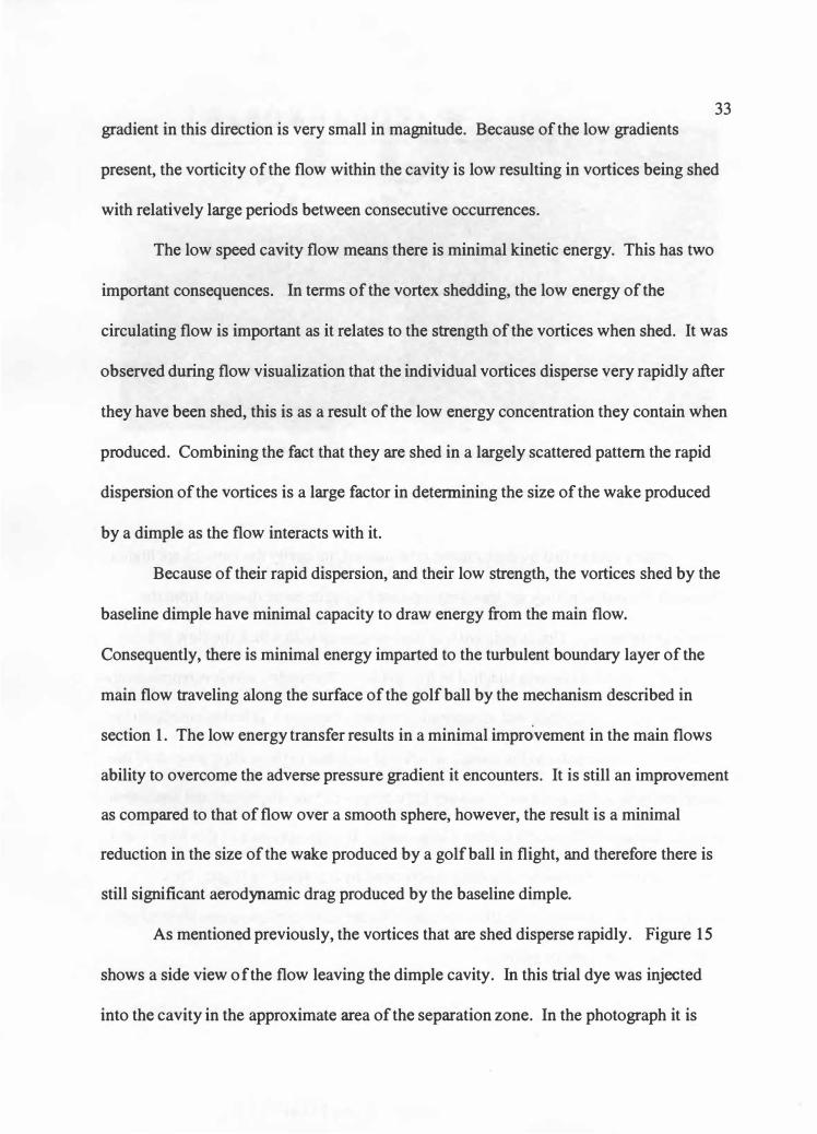
Figure 19: Fluid recirculation inside the Flat Dimple design 39

Figure 20: Pressure Data obtained for the flat bottomed dimple 40
Figure 21: Pressure Contour plot of Flat Dimple Design 41
Figure22: Improved flow attachment of the flat bottomed dimple 43
Figure 23: The dimple configuration containing a small insert 45
Figure 24: Improved circulation of this design 46
Figure 25: The pressure data collected for the dimple containing the small insert 47
Figure 26: Pressure contour plot of dimple with small insert 48
Figure 27: The increase size and turbulence of the wake created by this design is 51 apparent when compared to those of the previous configurations.
Figure 28: Dimple with large cavity insert 53
Figure 29: Recirculation around the large insert 54
Figure 30: Evidence of the forward stagnation point 55
Figure 31: Pressure data obtained for the dimple containing a large insert 56
Figure 32: Pressure contour plot of the dimple containing the large insert 57
Figure 33: The �educed wake and concentrated vortices shed from this design are 5 9 much improved over the previous designs.
Figure 34: The experimental Cp distribution compared to CFD results
Figure 35: The grid used for the CFD simulation.
Figure A-1: The middle of the support Structure
Figure A-2: The main support structure
Figure A-3: The baseline Dimple
Figure A-4: The flat Bottomed Dimple
Figure A-5: The Small Insert Dimple
Figure A-6: The Large Insert Dimple
60
62
69
69
70
70
71
71
vu

vm Nomenclature
(J) Vorticity
u Local Velocity
'\) Kin�matic Viscosity
Voo Free Stream Velocity
Poo Free Steam Pressure
p Local Pressure
Cp Coefficient of Pressure
Re Reynolds Number
p Density
k Dimple Depth
C Dimple Diameter
d Golf Ball Diameter

1-1: Introduction
Chapter 1
Introduction
1
Over the last several years the golf ball and clubs manufacturing industry has
expended considerable resources in efforts to improve the distance balls will travel when
hit by players. Much of these efforts have focused on the manufacturing of the clubs
used, including the materials used and the design of the clubs and balls. In the past, it has
been difficult to improve the aerodynamic efficiency of golf balls as testing was, and
remains, very costly and techniques used for modeling lacked the necessary
sophistication to provide accurate results. It has only been very recently, with the advent
of more sophisticated computer technology resulting in more sophisticated computational
fluid dynamics (CFD) models and improvements in experimental data collection that the
focus on reducing the drag produced by a ball in flight has been explored in great detail.
The complexity of a golf ball in flight makes it scientifically interesting.
Comparing a CFO model of a golf ball to experimental data, obtained through several
means including water or wind tunnel testing, provides a meaningful validation of the
ability of the model to predict the behavior of other relatively more complex systems.
For example, NASA has employed the modeling of a golf ball to predict the behavior of
the fuel tanks on the Space Shuttle 1• Reducing the drag of a golf ball through the
alteration of the dimpling has applications in areas such as improving the aerodynamic
performance of bridge girders and other similar support structures used in construction
areas subject to high wind loading2• Other studies have been performed to determine the
exact extent to which the dimples of a ball affect its flight and this has led to a greater

understanding of the fundamental principles that are at work. By way of example,
Takeyoshi and Tsutahra found that the angle with which a scratch on a ball's surface
interacted with the airflow had a significant impact on the behavior of the flow traveling
over the scratch.3
The present study is intended as an initial step in a series aimed at reducing the
aerodynamic drag produced by a golf ball in flight by experimenting with different
dimple shapes that have been designed from a fundamental point of view. Further work
would need to be carried out to optimize the distribution of the dimples. Study of the
distribution pattern is outside the scope of this project. The results published by Ting 4,
were used as a basis for further optimization of the dimples to decrease the drag
experienced by a ball in flight. The goal of this work is to experiment with various
selected shapes and to develop an improved dimple that possibly shows a reduction in the
drag produced by the dimples of a golf ball as it is in flight. It is also hoped that these
results can be used in other applications where dimple-like structures can be used to
reduce the amount of drag produced, and hence reduce the effect of many of the problems
associated with aerodynamic drag production in such applications.
This study combines the results of water tunnel flow visualization and pressure
measurements to understand the flow around a golf ball dimple. The Computational
Fluid Dynamics code CFO-ACE® was used as a tool to evaluate the results obtained for
an innovative dimple design that shows improvements in aerodynamic performance.
3 Chapter 2
Literature Review and Background
2-1 Literature Review
An extensive review of the literature associated with the design of dimples and
reduction in golf ball drag was carried out. Details were difficult to obtain because most
of the work that has been conducted in the industry is proprietary and not available for
review. However, some academic work has been conducted and this was the focus of the
literature research. In particular, the work carried out by L.L. Ting 4 and his associates
using CFD modeling techniques is referred to in this work. In his work, Ting first
demonstrated that the CFD code FLUENT® successfully modeled the flow over a
conventional golf ball5• Then he proceeded to use the codes to study the effects of
altering the depth and diameter of the dimples in order to determine each parameters
independent effect on the coefficient of drag (Co) experienced by the ball as a result of its
motion through the air. He did not however validate these results through
experimentation, relying on the previous validation of the CFD model chosen as
sufficient validation3•
Several Patents were also studied in order to begin the design process. Several of
the patents obtained are currently used by the golf ball manufactures Titleist, Callaway
and Wilson and are available in references 15, 16 and 18 respectively.
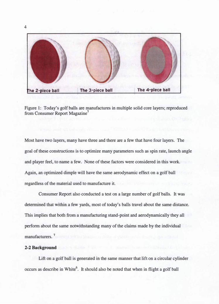
Interestingly, much more money is spent at present on the internal construction of
today's golf balls than the aerodynamics. As in figure 1, which was reproduced from
Consumer Report Magazine, nearly all of today's balls are multi-layer solid core balls.7
4
h• 2· lee• bal I The 3• pi C ball The 4·plec• baU
Figure 1: Today's golf balls are manufactures in multiple solid core layers; reproduced from Consumer Report Magazine 7
Most have two layers, many have three and there are a few that have four layers. The
goal of these constructions is to optimize many parameters such as spin rate, launch angle
and player feel, to name a few. None of these factors were considered in this work.
Again, an optimized dimple will have the same aerodynamic effect on a golf ball
regardless of the material used to manufacture it.
Consumer Report also conducted a test on a large number of golf balls. It was
determined that within a few yards, most of today's balls travel about the same distance.
This implies that both from a manufacturing stand-point and aerodynamically they all
perform about the same notwithstanding many of the claims made by the individual
manufacturers. 7
2-2 Background
Lift on a golf ball is generated in the same manner that lift on a circular cylinder
occurs as describe in White6• It should also be noted that when in flight a golf ball

5 generates backspin. The backspin is responsible for 20-25% of the lift. However, Ting
investigated the effect of backspin in his work. It was concluded that there was no
significant effect on drag caused by the backspin.4 In other words, if a dimple reduces the
drag, it will do so whether there is backspin present or not. In light of this, backspin was
not considered in this work.
Dimples are an essential component of golf ball design. Optimizing the
performance of the dimples has the goal of reducing the total drag coefficient
experienced by the ball. Consider a fluid flowing over a smooth spherical object as in
figure 2 such that starting at the leading edge stagnation point the flow over the surface of
the sphere results in a laminar boundary layer. As the flow travels over the surface of the
sphere it encounters an adverse pressure gradient created by the rear stagnation point.
The adverse pressure gradient causes the flow to separate readily from the sphere, which
in tum creates a large wake behind the sphere resulting in significant drag. 6
Figure 2: Flow over a smooth sphere; reproduced from reference 25.

Now consider the case of a sphere containing dimples on its surface. As the
fluid flows over the surface of the sphere it encounters the leading edge of the dimple as
shown in figure 3.
As the fluid enters the dimple a high pressure near stagnation condition exists at
the trailing edge. The pressure differential between the trailing edge region and leading
edge region causes the fluid to circulate within the dimple and a cavity flow exists.
Referring to figure 4, The main flow passes over the cavity, while some enters the cavity
and circulates. The creation of turbulence caused by the cavity is the mechanism that
allows energy from the main flow to pass on to the boundary layer past the cavity. The
turbulence is a result of vortex shedding occurring within the cavity. The flow entering
the cavity has a given amount of energy determined by the main flow. Circulation within
the cavity takes place, and vorticity is present. Vortices are shed, with a strength
determined by the velocity gradients present in the cavity.
Figure 3: Flow within a dimple cavity.

Separating Sf-_ r.-eam.l i. ne
/--J
1-1:::::) --�
�irculating Cav..ity Flow
Figure 4: Flow over a dimple; reproduced from reference 2.
7
Higher kinetic energy within the cavity flow results in higher energy, more
concentrated vortices with lesser dispersion upon leaving the cavity. Less dispersion
coupled with higher energy vortices result in vortices with a greater ability to draw
energy from the main flow as they leave the dimple cavities and mixing of the two flows
occurs. The energy drawn out of the main flow is imparted to the boundary layer along
the surface of the golf ball through this process. This energized boundary layer is better
able to resist the adverse pressure gradient it encounters as it travels along the surface of
the ball and encounters the increasing pressure. Because of the turbulence created by the
vortex shedding, nearly all references today refer to this type of boundary layer as a
turbulent boundary layer.6 While locally, a turbulent boundary layer creates more drag
than a laminar one, globally the flow remaining attached longer reduces the size of the
turbulent wake behind the ball, and thus an overall smaller wake and reduction in drag
occurs. 19
While the kinetic energy gradients determines the strength of the vortex shed, the
amount of vorticity present in a flow, and in tum the vorticity distribution, depends
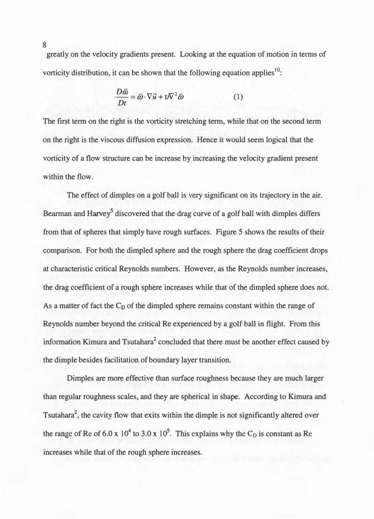
greatly on the velocity gradients present. Looking at the equation of motion in terms of
vorticity distribution, it can be shown that the following equation applies 10:
DiiJ - v- n2--=0J· u+Vv OJ Dt
(1)
The first term on the right is the vorticity stretching term, while that on the second term
on the right is the viscous diffusion expression. Hence it would seem logical that the
vorticity of a flow structure can be increase by increasing the velocity gradient present
within the flow.
The effect of dimples on a golf ball is very significant on its trajectory in the air.
Bearman and Harvef discovered that the drag curve of a golf ball with dimples differs
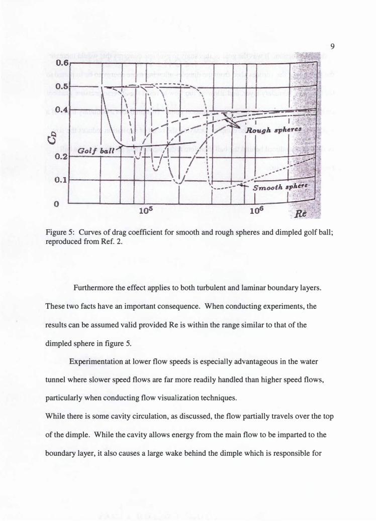
from that of spheres that simply have rough surfaces. Figure 5 shows the results of their
comparison. For both the dimpled sphere and the rough sphere the drag coefficient drops
at characteristic critical Reynolds numbers. However, as the Reynolds number increases,
the drag coefficient of a rough sphere increases while that of the dimpled sphere does not.
As a matter of fact the C0 of the dimpled sphere remains constant within the range of
Reynolds number beyond the critical Re experienced by a golf ball in flight. From this
information Kimura and Tsutahara2 concluded that there must be another effect caused by
the dimple besides facilitation of boundary layer transition.
Dimples are more effective than surface roughness because they are much larger
than regular roughness scales, and they are spherical in shape. According to Kimura and
Tsutahara2, the cavity flow that exits within the dimple is not significantly altered over
the range of Re of 6.0 x 10⁴ to 3.0 x 10⁵. This explains why the Co is constant as Re
increases while that of the rough sphere increases.
9
0.51----
JU. Figure 5: Curves of drag coefficient for smooth and rough spheres and dimpled golf ball; reproduced from Ref. 2.
Furthermore the effect applies to both turbulent and laminar boundary layers.
These two facts have an important consequence. When conducting experiments, the
results can be assumed valid provided Re is within the range similar to that of the
dimpled sphere in figure 5.
Experimentation at lower flow speeds is especially advantageous in the water
tunnel where slower speed flows are far more readily handled than higher speed flows,
particularly when conducting flow visualization techniques.
While there is some cavity circulation, as discussed, the flow partially travels over the top
of the dimple. While the cavity allows energy from the main flow to be imparted to the
boundary layer, it also causes a large wake behind the dimple which is responsible for

10 drag production. It was the goal of this study to evaluate concepts that would increase
the strength of the vortices shed from the dimples allowing more energy to be imparted to
the turbulent boundary layer, and allowing the flow to resist the adverse pressure gradient
caused by the ball's wake flow rear stagnation point. This produces a boundary layer of a
much fuller profile rear of the dimple. Delaying the onset of separation reduces the size
of the wake produced behind the ball therefore reducing the drag produced as the ball
flies through the air.

3-1 Introduction
11 Chapter 3
Experimental Approach
In attempting to optimize the dimple design, the goal is to delay the onset of flow
separation for as long as possible in order to reduce the drag coefficient. In a practical
sense this will allow the ball to travel further given the same (flow) conditions.
Using the FLUENT CFO code Ting and his associates found an optimal dimple
depth (k) of 0.008587 inches and an optimal dimple diameter (C) of 0. 1368 inches.
Using the golf ball's diameter (d) to form dimensionless parameters, these values
corresponded to a kid of 0.005 and c/d of 0.083• The dimple described here is the one
that was first tested as a baseline for comparison when considering the results of other
dimple shapes. In order to vary only one parameter, the diameter and depth of dimples
used for testing never changed as it was assumed that these optimal values of depth and
diameter would remain so regardless of the shape of dimple employed. Note that in his
work Ting discovered that beyond the optimal value quoted here, further increasing the
dimple depth had no effect on C0•
3-2 Dimensionless Modeling
In order to develop a scale model, an estimate of the Reynolds number
experienced by a golf ball in flight was required. Using ACCUSPORTS VECTOR
LAUNCH MONITOR©, representative ball launch conditions were obtained. The
conditions in table 1 were obtained. In its operation, a golf ball travels through a series of
highly sensitive lasers. The launch monitor determines the ball's velocity at impact, spin
rate and club head speed and determines the distance traveled from the data. 23 The initial

12
Table 1: Launch Conditions
Initial ball velocity 155 miles/hr Club Head Speed 1 15 miles/hr Backspin Rate 2800 rev/min
ball velocity corresponds to a Reynolds Number (Re) of 2.033 x 10⁵ with the diameter of
a regular golf ball dimple (0. 137 inches) as the characteristic length. The numbers
shown in Table 1 are representative of the author's golf swing, which falls well into the
average numbers of amateur golfers. It should be recognized that professionals have
higher numbers while other people are below these numbers. However, in each case the
numbers will vary by no more than 20%, placing the range of possible Re well within the
limits discussed in reference to figure 524•
Early on in this work it was recognized that testing a dimple that would be the
actual size of that found on a golf ball would be extremely difficult. It was also
recognized that a water tunnel would be preferable for flow visualization measurements
due to the ease of flow visualization techniques. In order to facilitate testing, scaling of
the models would be required using the dimensionless relations kid and c/d as per Ting's
paper. It was decided that a dimple diameter of 5 inches would be appropriate as it would
allow for ease of testing. As such scaling of the model for the water tunnel using the
Reynolds number and the dimensionless parameters used by Ting was carried out with
the resulting scaled parameters listed in table 2. Note that the actual diameter (d) of a
golf ball used for play in golf is 1. 7 17 inches. 4
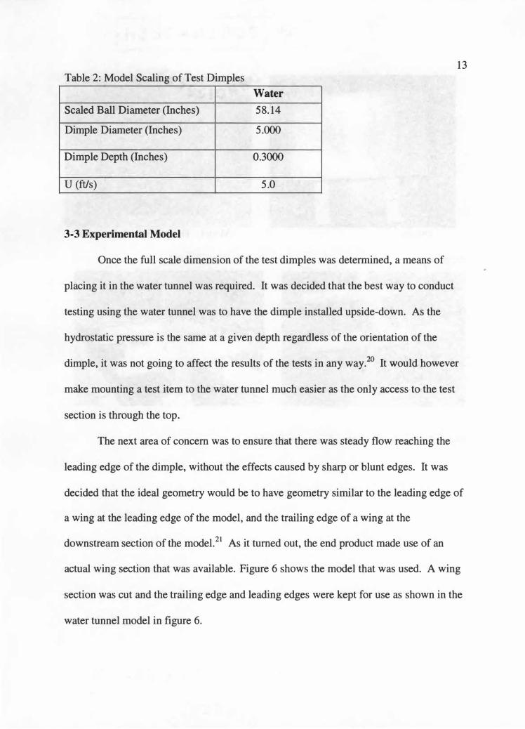
13 Table 2: Model Scaling of Test Dimples
Water
Scaled Ball Diameter (Inches) 58. 14
Dimple Diameter (Inches) 5.000
Dimple Depth (Inches) 0.3000
U (ft/s) 5.0
3-3 Experimental Model
Once the full scale dimension of the test dimples was determined, a means of
placing it in the water tunnel was required. It was decided that the best way to conduct
testing using the water tunnel was to have the dimple installed upside-down. As the
hydrostatic pressure is the same at a given depth regardless of the orientation of the
dimple, it was not going to affect the results of the tests in any way. 20 It would however
make mounting a test item to the water tunnel much easier as the only access to the test
section is through the top.
The next area of concern was to ensure that there was steady flow reaching the
leading edge of the dimple, without the effects caused by sharp or blunt edges. It was
decided that the ideal geometry would be to have geometry similar to the leading edge of
a wing at the leading edge of the model, and the trailing edge of a wing at the
downstream section of the model. 21 As it turned out, the end product made use of an
actual wing section that was available. Figure 6 shows the model that was used. A wing
section was cut and the trailing edge and leading edges were kept for use as shown in the
water tunnel model in figure 6.
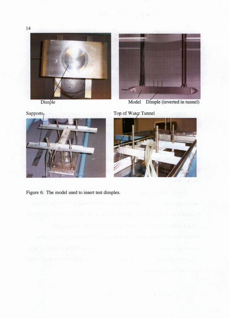
14
Figure 6: The model used to insert test dimples.
Model Dimple (inverted in tunnel)

15 A solid block was then designed, and the center was cut out so that the test dimples
could be inserted. The wing sections were then attached to the block to obtain the model
shown in figure 6. The engineering drawings for the main block are included in appendix
A, figure A-1 and the block and wing section in A-2.
The Drawing in figure A-1 also shows how the dimple was inserted. The hole in
the top was stepped, and the dimple inserts themselves were stepped so that they would
fit in. The dimple engineering drawings are included in figures A-3 through A-6. The
opening in the main model was cut so that the dimple model would fit tightly, but would
still be able to rotate. In order to hold the dimple in place once it had been rotated, a plate
was attached to the top (towards the top of the tunnel) of the dimple insert through the
use of screws which was graduated every ten degrees. With the model installed in the
water tunnel, rotating the dimple was simply a matter of loosening the screws, rotating
the dimple insert and re-tightening the screws. This allowed testing to occur efficiently.
Changing the dimple insert was a matter of taking the screws out completely, removing
the insert, and inserting the new one with the plate and the screws.
Each dimple cavity had pressure ports drilled out as per the dimensions in figures
A-2 through A-5. These came through the top of the cavity, and the pressure hoses were
connected to them at the top. This allowed the user to simply remove them before
removing an insert, and simple reattachment once the new dimple insert was installed.
Figure 6 also shows how the model was mounted to the water tunnel. Four large
bars were screwed into the top of the model at each of the four comers. The bars were of
sufficient size and strength that they were not affected by the loads placed on them by the
water flowing through the tunnel, ensuring that the model did not move or vibrate during
16 testing. A beam was placed connecting each span-wise pair of bars. With the beam in
place the model would be held stationary by the top of the water tunnel test section.
3-4 Flow Visualization
As alluded to previously, in order to carry out some quantitative measurements
using flow visualization techniques the water tunnel facility at the University of
Tennessee Space Institute (UTSI) was employed. The water tunnel was the preferred
facility as it far more readily facilitated flow visualization than the low speed wind tunnel
facility that was also available. The water tunnel facility at UTSI, capable of a
maximum flow speed of three feet per second was used for both flow visualization and
pressure measurements.
After some trials, however, it was found at the higher range of velocities a large
standing wave is generated which posed two significant problems. The first and most
significant is that with the relatively large standing wave generated, static and total
pressure measurements would be difficult to obtain. The range of expected pressure
measurements is ±1-3 inches of water. A large standing wave, in this case on the order of
three inches or more, would introduce significant error to the measurements. The second
problem posed by the standing wave is that it introduces a disturbance at depths where
the model is located. This makes flow visualization very difficult as the dye stream is
affected by the disturbance created by the standing wave. Flow speed of approximately 1
foot per second was settled upon after some trial and error. This places the Re at 6.7x10⁴
still within the range of constant Co found by Kimura and Tsutahara2. Further supporting
this decision was the work carried out by McDaniels in a similar facility at UTSI. In his
17 work, McDaniels found that in modeling a higher Re flow with a lower Re flow, the
qualitative details remain in tact. 14
The dye selected to carry out the flow visualization observations was formulated
to be neutral density with respect to the water in terms of specific gravity. This made the
dye neutrally buoyant allowing for proper boundary layer observations to be undertaken.
Before measurements were made, the density of the dye was tested to ensure that it was
in fact the same as the water. As a matter of detail, the color of the dye used was changed
so that it would show up better in pictures. This did not however change the
composition of the dye nor its buoyancy.
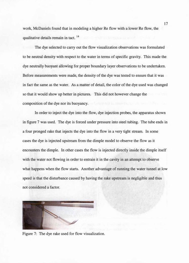
In order to inject the dye into the flow, dye injection probes, the apparatus shown
in figure 7 was used. The dye is forced under pressure into steel tubing. The tube ends in
a four pronged rake that injects the dye into the flow in a very tight stream. In some
cases the dye is injected upstream from the dimple model to observe the flow as it
encounters the dimple. In other cases the flow is injected directly inside the dimple itself
with the water not flowing in order to entrain it in the cavity in an attempt to observe
what happens when the flow starts. Another advantage of running the water tunnel at low
speed is that the disturbance caused by having the rake upstream is negligible and thus
not considered a factor.
Figure 7: The dye rake used for flow visualization.

18 3-5 Pressure Measurement
In order to obtain an estimate of the pressure variations within the dimple, it was
decided to drill three small pressure ports into the cavity as shown in figure 8. Connected
through tubes coming out of the top of the model to pressure transducers, the pressure
was measured at each of the three locations. By rotating the dimple in ten degree
increments a distribution of the pressure within the complete cavity was obtained.
Finding suitable pressure transducers proved to be difficult.
Initially pressure transducers where installed such that water entered partially in the tube
and would cause the air pressure at the transducer to increase. This however produced
unacceptable unstable results. As mentioned, the expected range of pressure
measurements was on the order of ± 1-3 inches of water.
Figure 8: Distribution of holes used to measure the pressure inside the cavity and the method used to connect the pressure transducers.

19 The problem with this set up was that the tubes that were used were very small and the
water would not completely drain from them. The water that remained in the tube was
enough to cause a 40-50% error as compared to the value measured. This was not
acceptable.
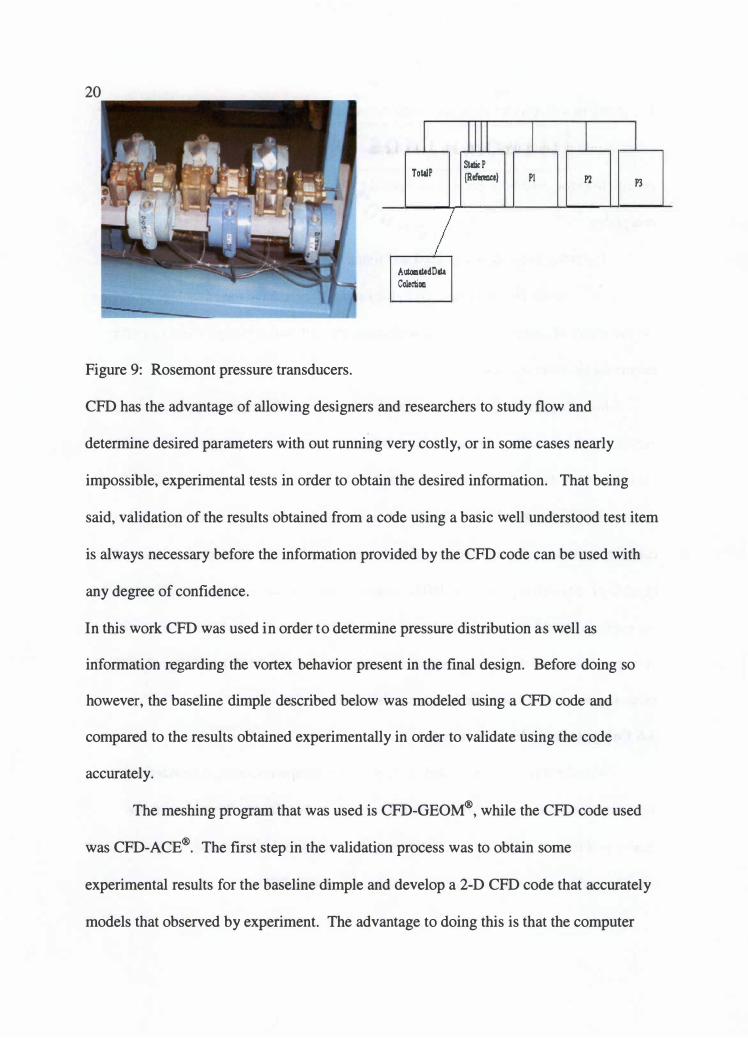
The setup in figure 9 was tried and found to be successful. In this set up
Rosemont® transducers are connected to the tubing. These have the advantage of having
the capability of coming into contact with water thus alleviating the problem caused by
having an air water interface.
Initially pressure transducers whereby the water in the tube would cause the air
pressure at the transducer obtained the coefficient of pressure and distribution could be
obtained. This data could then be compared to the results of the computation fluid
dynamics code discussed later. The Rosemount transducers were spanned so that they
could measure the pressure from negative ± 3 inches of water. The transducers are also
capable of measuring pressure to 0.001 inches of water. It was estimated that the error in
the readings provided by the transducers was ± 0.5% of maximum range. The automated
system collected 10 data points per second, each an average of 1000 readings. The Root
mean squared method was used to obtain the error estimates. 12
3-6 Computational Fluid Dynamics
With the advent of faster and more powerful computers, computational fluid
dynamics is now at the forefront of fluid dynamics study. Simple flows such as the
classic problem of flow over a cylinder to much more complex ones describing the flow
over the entire surface of an aircraft can be modeled with CFD.
20
Figure 9: Rosemont pressure transducers.
ToltlP
Automated011e.
ColectiOG
Static P {Refemlce} Pl P2 P3
CFD has the advantage of allowing designers and researchers to study flow and
determine desired parameters with out running very costly, or in some cases nearly
impossible, experimental tests in order to obtain the desired information. That being
said, validation of the results obtained from a code using a basic well understood test item
is always necessary before the information provided by the CFD code can be used with
any degree of confidence.
In this work CFD was used in order to determine pressure distribution as well as
information regarding the vortex behavior present in the final design. Before doing so
however, the baseline dimple described below was modeled using a CFD code and
compared to the results obtained experimentally in order to validate using the code
accurately.
The meshing program that was used is CFD-GEOM®, while the CFD code used
was CFD-ACE®. The first step in the validation process was to obtain some
experimental results for the baseline dimple and develop a 2-D CFD code that accurate! y
models that observed by experiment. The advantage to doing this is that the computer

21 processing required to run a 2-D code is far less than that of a 3-D code, and therefore
trouble shooting and variation of the numerous parameters associated with the code can
be carried out far more quickly.
Once an acceptable 2-D code was developed and results found to satisfactorily
model what was observed by experimentation, a 3-D code was used to complete the
validation process. The 3-D code is processor intensive and requires a lengthy amount of
time to run. However, once the various parameters have been adjusted properly, the
resulting 3-D model provides an excellent tool for studying the expected pressure
velocity and vorticity distributions. Of course, the results obtained using the 3-D code
was once again checked to ensure that they accurately reflected the observed phenomena.
Once the baseline code provided satisfactory results, it was used to model the
flow parameters of the final design, the large mountain dimple described below. Those
results that could be obtained experimentally were compared to ensure the model
accuracy in order to determine is viability as a means of studying future designs.
3-7 Dimple Design
As mentioned in an earlier section, golf ball dimples are designed such that there
exists an internal cavity flow. Many studies have been conduced that changed the depth,
diameter and the distribution of dimples on a golf ball, including the work done by Ting 4
and his associates. In addition, the Callaway and the Wilson companies have developed
dimples of hexagonal and flat-bottomed shapes respectively as outlined by the patents in
references 15 and 16. Despite this effort, independent testing such as those carried out by
Consumer Reports magazine in reference 7 discussed previously have shown that
aerodynamically, all of these balls perform nearly equally.

22 In order to improve the aerodynamic performance of a dimple, one may
conclude that a fundamental change in the behavior of the flow inside and within the
vicinity of the dimple is required.
As discussed in reference 2, there is a portion of the flow that passes over the
dimple while a small portion of the flow is brought into the dimple where the action of its
circulating within the cavity helps to re-energize the flow passing over the cavity. The
increased energy allows the flow to remain attached to the surface of the golf ball more
readily once it passes the dimple as it is better able to resist the adverse pressure gradient
created by the balls aft stagnation point. 6 The global effect is that the flow over the
sphere remains attached longer and the size of the wake behind the ball is reduced, thus
reducing the drag. 6 In considering different design possibilities, the goal is to impart as
much energy to the boundary layer of the main flow after passing over the cavity as
possible. Even a modest increase in the energy imparted to the flow on the order of 10-
20% can significantly reduce the aerodynamic drag produced by a dimple as this
represents a large increase in the flow's ability to overcome adverse pressure gradients.6
At the leading edge of a dimple the flow coming from upstream separates from
the surface of the ball. The majority flow continues over the dimple while a very small
portion of it circulates inside the cavity. In order to increase the amount of energy
imparted to the main flow boundary layer, it would be desirable to increase the strength
of the vortices shed from the cavity. To accomplish this, the local velocities and velocity
gradients inside the cavity must be increased. As discussed before, this has the effect of
reducing the wake both aft of the dimple and globally.2

23
In order to have the flow reattach to the surface of the sphere, it was
hypothesized20 that a "insert" centered over the center of the dimple cavity would provide
a surface for the flow to reattach to. With the larger surface of the insert providing a
means of attaching the flow, it was supposed that a greater portion of the total flow
passing over the cavity will be brought in and move around the insert. Attaching to the
surface of a insert also increases the velocity of the flow circulating within the cavity and
increasing the kinetic energy available. It was hypothesized that the mixing of the two
flows would increase the energy of the flow beyond the dimple thus allowing the flow to
remain attached to the surface of the golf ball, and reducing the drag. 2
While ideally the insert could extend higher than the leading edge surface of the
diameter of the ball, practically this is not possible. During the contact between the golf
club and the ball, a large amount of deformation takes place due to the significant amount
of force that is involved. Because of this, having the insert extend outside of the cavity
would mean that within a small number of strikes, the insert would lose its effectiveness
as it would be crushed or damaged in some fashion.
In order to test the effects of a insert inside the cavity, four dimples were built.
The first one was a standard scaled dimple shape with the optimal depth and diameter
that was determined by Ting.4 In order to reduce the number of variables involved, this
was also the depth and diameter of each of the test dimples studied. The second dimple
studied was based on the patent in reference 18 produced by Wilson. In this design, the
bottom of the cavity is flat similar to a frying pan. In the patent, the designer of the
dimple states that it shows improved performance over a standard shaped dimple in that it
reduced the overall drag produced. 18 The third dimple was built having a mountain insert

24 in the cavity that extends to 0.05" below the top of the dimple cavity, with a top
diameter of 0.25" and the sides sloping 45°. The final dimple was similar to the third;
however the top diameter of the mountain was increased to one inch. It was hoped that
these configurations could be compared to both the baseline dimple and the flat bottomed
dimple and would show improvement in terms of the size of the wake generated as the
flow leaves the cavity.
Finding suitable pressure transducers proved to be difficult. Initially pressure transducers
whereby the water in the tube would cause the air pressure at the transducer to increase
were tried. This however produced unacceptable results. As mentioned, the expected
range of pressure measurements was on the order of ± 1-3 inches of water.
3-8 Notes Regarding Co Measurement
Unfortunately, it is impossible to directly measure the coefficient of drag with the
resources available at UTSI. However, using flow visualization it is possible to obtain a
qualitative assessment of whether or not the aerodynamic drag wake behind the dimple is
reduced or not. Observations such as the size of the wake, the amount of flow brought
into the cavity and the degree to which the flow remains attached to the surface after the
dimple can be compared amongst the various models. While these types of observations
are valuable, highly accurate measurements would be preferable but are not possible due
to resource limitations. The information obtained is still important as it may help
determine whether future, more costly, testing is warranted.
Measuring the pressure distribution within the cavity is in contrast very accurate,
and provides a direct quantitative comparison of the performance of each cavity through
the use of non-dimensional coefficients, namely the pressure coefficient.

25 The CFD code also provides a very accurate comparison of the performance of
each respective cavity in addition to providing an excellent means of validating the
results obtained experimentally.

26
Chapter 4
Experimental Results and Discussion
4-1 Flow Visualization Notes
The dye used to carry out the flow visualization experiments is a mixture of
ethanol, short-chain polymer, and water. The ingredients are mixed in proportions
necessary to ensure the specific gravity is as close to water as possible. Prior to running
the experiments, it was important to ensure that the dye used was neutrally buoyant with
respect to the water in the tank. In order to test the dye, the water tunnel was turned off
and sufficient time was allowed for the water to settle. A drop of dye was placed in the
tunnel. If it sank, its specific gravity was high and ethanol was added to reduce the
specific gravity. If it rose, polymer was added. This adjusting process continued until
the drop would remain still in the water, indicative of it having the appropriate specific
gravity.
Because of some problems associated with running the tunnel at higher speeds,
namely the presence of a standing wave at higher speeds, and that slower water speeds
facilitate visualization, the tunnel was adjusted such that the flow velocity was
approximately one foot per second. Note that this places Re at approximately 6.7 x 10⁴,
within the range studied by Kimura and Tsutahara2 as discussed earlier. The pressure
measurements were conducted at approximately 2.0 feet per second. This was necessary
in order to have pressure values within the range the transducers were capable of
measuring with accuracy. As per the previous discussion, the visualization observations
made would still be valid at this speed.

27 4-2 Baseline Dimple
The first dimple shape studied was the one shown in figure 10. The spherical
shape of the cavity itself is based on the current design patent in reference 15 which is
currently in use by the Titleist Company as the standard dimple shape in its golf balls.
The design was altered slightly using the results that Ting and his associates obtained.
The optimal depth and diameter quoted in Ting's work was selected as it represented the
configuration that produced the least amount of drag. A more meaningful comparison of
the performance of the designs obtained in this work could be achieved in this manner.
In order to study the recirculation inside the dimple cavity the dye probes were
placed inside the cavity such that they were in contact with the surface. With the flow
running dye was injected into the dimple and the streaklines were digitally recorded.
Figure 11 shows a still image taken from one of the videos. There is a small region of
recirculation occurring in the dimple. Within a short distance from the dimple beginning,
there are vortices shed and the flow is separated and leaves the cavity.
Figure 10: The baseline dimple.
28
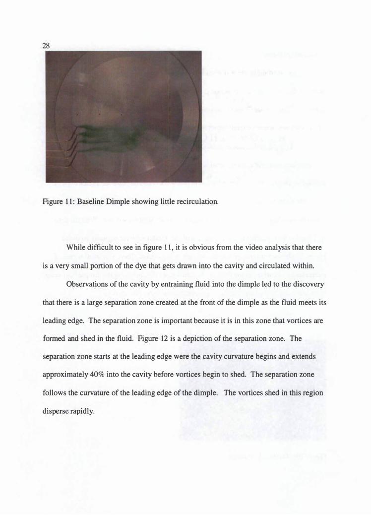
Figure 11: Baseline Dimple showing little recirculation.
While difficult to see in figure 11, it is obvious from the video analysis that there
is a very small portion of the dye that gets drawn into the cavity and circulated within.
Observations of the cavity by entraining fluid into the dimple led to the discovery
that there is a large separation zone created at the front of the dimple as the fluid meets its
leading edge. The separation zone is important because it is in this zone that vortices are
formed and shed in the fluid. Figure 12 is a depiction of the separation zone. The
separation zone starts at the leading edge were the cavity curvature begins and extends
approximately 40% into the cavity before vortices begin to shed. The separation zone
follows the curvature of the leading edge of the dimple. The vortices shed in this region
disperse rapidly.

29
Figure 12: A schematic of the separation zone and associated vortex shedding
At first it was not known why so little of the flow was being drawn into the
cavity. However, study of the pressure distribution within the dimple provided the
answer. Figure 13 is a plot of the data that was obtained by measuring the pressure
within the cavity and calculating the coefficient of pressure (Cp ). As a matter of
reference CPI is the data that was collected from the pressure port 2.25 inches from the
center of the cavity, while CP2 and CP3 were measured moving inward toward the center
as per figure 8. The data was collected in 10 degree intervals along the 360 degree
circular cavity. It can be seen from the plot that CP3 remains nearly constant except for
the region between 130 degrees and 280 degrees where there is a sharp increase in the
value of CP3. Cp is defines as follows:
(2)

30
- C P1 CP Va Position _Baae line - cP2
C P3
0.35
0.3
0 .25
0.2
0.1 5
0.1
0 .05
0
-0.05
-0. 1
Poaltlon (ct.gr•••>
Figure 13: Pressure data obtained inside the baseline cavity.
The increase is on the order of 20%, which reflects a drop in the velocity of the fluid in
the cavity in this region. This also marks a region where flow separation has increased.
Note that this region is fairly large. CPI varies from nearly zero, with peaks occurring at
approximately 100 and 250 degrees with a valley near 180 degrees. The peaks are areas
were separation is centered, hence the higher value in CP while the valley represents a
region where flow circulation and vortex shedding is occurring. CP 2 shows a similar
trend with higher overall values of the coefficient of pressure as CP2 is more inside the
separation bubble. There is an asymmetric behavior though to be due to flow alignment
relative to the model axis may not have been exact.
The contour plot in figure 14 was obtained by taking the pressure measurement
data from figure 13 and interpolating it to cover the entire surface of the cavity. The
interpolation does introduce some uncertainty into the plot. However, comparison of the
visual observations made from figure 11, and the CFD results, discussed later show good
agreement. The black dots represent actual data points.
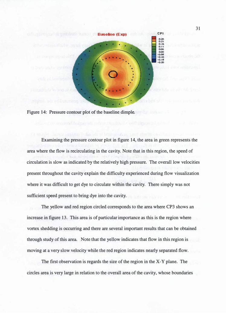
Baselne (Exp)
Figure 14: Pressure contour plot of the baseline dimple.
C P 1
0.::6 0.:?I 0.16 0.1 1 0.0& 0.00
-0.05 -0.10 -0.15 -0.20
31
Examining the pressure contour plot in figure 14, the area in green represents the
area where the flow is recirculating in the cavity. Note that in this region, the speed of
circulation is slow as indicated by the relatively high pressure. The overall low velocities
present throughout the cavity explain the difficulty experienced during flow visualization
where it was difficult to get dye to circulate within the cavity. There simply was not
sufficient speed present to bring dye into the cavity.
The yellow and red region circled corresponds to the area where CP3 shows an
increase in figure 13. This area is of particular importance as this is the region where
vortex shedding is occurring and there are several important results that can be obtained
through study of this area. Note that the yellow indicates that flow in this region is
moving at a very slow velocity while the red region indicates nearly separated flow.
The first observation is regards the size of the region in the X-Y plane. The
circles area is very large in relation to the overall area of the cavity, whose boundaries

32
match those in the figure. As this is the region where vortex shedding is occurring, this
region shows that the zone in which separation occurs is very large, which agrees with
the observations made in flow visualization in figure 11 and 12. This large region of
separation zone indicates that the initial distribution pattern of the vortices when shed is
quite large, and therefore, regardless of their strength, will be quite dispersed as they
leave the cavity and mix with the main flow. This is important as it is one of the factors
that determine the size and effectiveness of the turbulent wake generated by the dimple.
Figure 14 contains information regarding the total vorticity of the flow in the
cavity. It was observed through flow visualization that the period between successive
vortices being shed is relatively long as compared to the other designs tested. Figure 13
explains in part why this is the case. The difference in velocities within the circled region
from one point to the next are not significantly high resulting in low velocity gradients.
Loo�ng once again at equation ( 1 ):
DiiJ - o- 0 2 -- = m· v u + vv (J) Dt
From this equation we can see that the rate of change of vorticity, described by the first
term on the right is highly dependent on the velocity gradients present. The gradients in
the X-Y plane are minimal as can be seen in figure 13. Also of interest is the velocity
gradient in the Z direction, defined for this work as the direction normal to the plane of
the cavity. In this direction the distance between the bottom of the cavity, approximately
where separation is occurring, and the main flow is nearly equal to the depth of the
cavity, in this case 0.30 inches. While the difference between the main flow velocity and
the re-circulation velocity may be high, the distance between them is small, and thus the
33 gradient in this direction is very small in magnitude. Because of the low gradients
present, the vorticity of the flow within the cavity is low resulting in vortices being shed
with relatively large periods between consecutive occurrences.
The low speed cavity flow means there is minimal kinetic energy. This has two
important consequences. In terms of the vortex shedding, the low energy of the
circulating flow is important as it relates to the strength of the vortices when shed. It was
observed during flow visualization that the individual vortices disperse very rapidly after
they have been shed, this is as a result of the low energy concentration they contain when
produced. Combining the fact that they are shed in a largely scattered pattern the rapid
dispersion of the vortices is a large factor in determining the size of the wake produced
by a dimple as the flow interacts with it.
Because of their rapid dispersion, and their low strength, the vortices shed by the
baseline dimple have minimal capacity to draw energy from the main flow.
Consequently, there is minimal energy imparted to the turbulent boundary layer of the
main flow traveling along the surface of the golf ball by the mechanism described in
section 1 . The low energy transfer results in a minimal improvement in the main flows
ability to overcome the adverse pressure gradient it encounters. It is still an improvement
as compared to that of flow over a smooth sphere, however, the result is a minimal
reduction in the size of the wake produced by a golf ball in flight, and therefore there is
still significant aerodynamic drag produced by the baseline dimple.
As mentioned previously, the vortices that are shed disperse rapidly. Figure 15
shows a side view of the flow leaving the dimple cavity. In this trial dye was injected
into the cavity in the approximate area of the separation zone. In the photograph it is

34
Figure 15: The dispersed wake generated behind the baseline dimple.
clearly visible that by the time the flow has left the cavity the vortices are highly
dispersed. In addition, they are traveling separated by quite some distance from the
surface of the model. This is indicative of the low energy with which the flow left the
cavity. It is unable to remain attached to the surface of the model, which is representative
of the surface of a golf ball, and so separation occurs. Because it is losing energy due to
the viscosity of the water in the tunnel, which was included in the scaling process of the
water, the flow at this point contains very little energy and the dispersion and separation
from the surface of the model creates a large wake. It is the presence of this large wake
that is responsible for most of the drag experienced by a golf ball in flight. This
experiment was run twice to confirm the results as the other configurations showed very
significant improvements in this area.

35 Figure 16 is a top view of the wake that is generated as a result of the flow interacting
with the cavity. Here the dye was introduced into the flow upstream of the leading edge.
The lines drawn are intended to bring to attention the size of the wake generated in
relation to the size of the dye stream fed into the flow. The ratio of the wake size to the
dye stream size was found to be approximately 1 .5. This is qualitatively significant as it
is apparent that the wake is substantially larger than the initial stream fed to the cavity.
While this wake is not as large and not as dispersed as it would be behind a smooth
sphere, it is still a significant source of drag production.
Figure 16 : The wake generated by the baseline dimple in relation to the size of the dye stream.

36
4-2-1 Simulation of the Dimple Flow Using CFD-ACE
CFD-Ace is a Navier-Stokes solver. Both unsteady and steady flow models were
studied. In the 2-D cases that were run unsteady flow was simulated. While this would
also have been appropriate, this was not possible due to the time required to run with the
computing resources that were available.
In the steady cases, the K-e turbulence model was used, while for the unsteady
cases, the Large Eddie Simulation (LES) turbulence model was used. In both cases the
turbulence intensity was set to 1 %. This parameter was studied through several trials and
1 % was the value found to provide results that best agreed with experimental data.
For the 2-D simulations, approximately 200,000 mesh points were required to
provide acceptable results that converged. For the 3-D case one million mesh points
were generated. This was the maximum allowable based on the computer resources
available. In order to use one million mesh points, only a portion of the geometry
including the dimple and a section of length and height equal to five times the dimple
diameter could be constructed. It was assumed this would remove any possibility solid
boundary effects. Figure 17 shows the complete 3-D geometry as well as a slice through
the cavity. Note the dense grid along the boundary layer in figure 17(b ).
Figure 17: The geometry used for the 3-D CFD simulations.

37 Figure 18 shows the pressure distribution inside the cavity obtained from
running a 3-D CFD code using CFD-ACE next to the same plot shown in figure 14. As
figure 18 shows, the results of the CFD analysis generally agrees very well with the
experimental results. The blue region on the leading and trailing edges of the plot
obtained through CFD are a result of a small region of flow separation due to the
geometrical discontinuity that exits only in the CFD model, and do not show up on the
experimental plot. The size overall size of the region in red, where vortex shedding
occurs, is nearly the same size in both plots. The CFD code predicts slightly slower
velocities around the outer edges of the dimple as the yellow region of the plot is
somewhat larger than that shown in the experimental plot. Note that the velocity
difference in the area is minimal. It is assumed that some of this difference is a result of
the interpolation process that was used to plot the experimental results.
Baselne (Exp) CP1
0.31,
O.:?I
0.16
0.1 1
0.0&
ODJ •O.QS
•O.IO
•0.15 - ·0.20
Baseline (CF D )
Figure 18: A comparison of the pressure distribution inside the cavity obtained experimentally and through the use of CFD.

38
However, it can be readily seen that the results shown here compare very well, indicating
that both the interpolation process and the CFD model can _be used to predict the flow.
Consequently, the experimental results obtained can be used with confidence. In
addition the CFD code can be used to obtain results that can not be obtained
experimentally with confidence that they will be sufficiently accurate to provide
meaningful information. It should be noted that the experiments conducted were an
unsteady process while the 3-D code was a steady simulation. If the code could have
been run with an unsteady model, the result would have been similar to that obtained with
some minor differences.
4-2 The Flat Bottom Dimple
The next dimple shape that was studied was the flat bottomed dimple, as patented
by Wilson in reference 19. As expected, there is a separation zone very similar to the one
for the baseline dimple. There is however a slight improvement in the amount of
recirculation that takes place inside the cavity.
Figure 19 shows two photos taken during the same trial at approximately a 35
second interval. It is clear from these two photos and from the video obtained that there
is circulation occurring, albeit slowly, within the cavity. The photographs in figure 19
represent visual confirmation of improvement of flow recirculation over the recirculation
observed in the baseline dimple. The improvement in visible circulation inside the cavity
is due to the slightly faster velocity of circulation as compared to the base dimple.
39
Figure 19: Fluid recirculation inside the Flat Dimple design.
The plot in figure 20 is the pressure coefficient data that was measured for this
configuration. It shows much of the same trends as the baseline dimple plot of figure 13
however, there are some notable differences. The most striking is the difference in the
behavior of CP3 near the center of the cavity. Whereas the baseline dimple showed a
marked peak, the plot in figure 20 shows a nearly constant value throughout.
In the region were the peak in the baseline CP3 occurs this configuration
represents a decrease in CP3 of approximately 20%, with a similar improvement in the
velocity of the circulation in this region, there is a definite improvement in this region in
terms of the circulation for this configuration. CPl displays little change from that of the
plot for the baseline. CP2 also shows a similar trend as that obtained for the baseline,
however there is a small increase in CP2 of about 15% around the 180 degree region in
this configuration.

40
Cp vs Pos ition _flat Dim ple
0.35 �--------------------------,
0.25
0. 1 5 --------------------�--------
4 0
-0.1 ,,.__ ___________ �-------------Pos ition ( De g re e s )
Figure 20: Pressure Data obtained for the flat bottomed dimple.
This is the rear region of the dimple cavity, and it is thought that this is due to more
concentrated separation taking place here.
The faster circulation velocity also allows more of the flow to be brought into the
dimple cavity from the main flow passing over the top as it results in a lower pressure in
the cavity, and therefore a higher pressure gradient between the cavity and the main flow.
Figure 21 is a pressure coefficient contour plot obtained from the pressure data
measured within the cavity. Again, the pressure data collected was used to interpolate the
plot over the entire surface of the dimple. It is, as was the case with the baseline dimple,
subject to some uncertainty, however, as discussed the results can be used with
reasonable confidence as they do reflect trends viewed visually.
F lat ( E >q>)
Figure 21: Pressure Contour plot of Flat Dimple Design.
0 33,
0 2 1
0 16
0 t i
D OG
0 00 •0 05
D 10 0 15
� 0 20
4 1
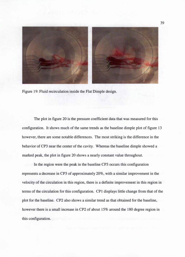
The area in yellow again represents low speed flow were some separation is
occurring. The region in red, representing high pressure is a result of the flow being
largely separated or stagnated. The red zone corresponds to the region in figure 18 where
CP2 and CP3 are higher than that of the baseline. It is within this region that the majority
of the separation and vortex shedding is occurring, thus the higher CP values. As can be
seen in figure 19, there is a change in the middle region of the cavity, circled, as
compared to the baseline cavity. It is evident that the pressure gradients have increased
somewhat, reflecting increased velocity gradients. The increased gradients present are
indicative of a minimal increase in the vorticity of the flow within the cavity. It was
visually observed that the vortices shed from this design were somewhat tighter and shed

42 with a minimally decreased period as compared to the baseline. This is a factor in the
reduction of the wake produced behind this dimple design. While this represents a slight
improvement over the baseline dimple note that the separation zone is still relatively
large, and thus a large wake is expected based on this observation.
Note that the red region where separation has occurred is somewhat more
concentrated than that of the baseline dimple, indicative of a more concentrated initial
distribution among the vortices when initially shed. The effect is not as apparent with
this design as in following ones, however there is some improvement. This allows the
vortices to have a lesser dispersion as they leave the dimple, contributing again to a
reduction in the size of the wake produced by this configuration.
The higher kinetic energy of the flow in the region where vortex shedding is
occurring, the vortices shed with a higher energy and therefore increased strength. This
increase strength coupled with the reduction in initial dispersion allows the vortices to
disperse less quickly. More importantly however, the increase strength of the vortices
allows them to draw more energy from the main flow and thus the turbulent boundary
layer receives greater energy as a result. This improves the overall ability of the flow to
remain attached to the surface, and the wake production behind a golf ball would be
reduced as a result. It would seem that the claim made by the designer of this
configuration in reference 19 would indeed seem valid as a reduction in aerodynamic
drag production would be expected based on this.
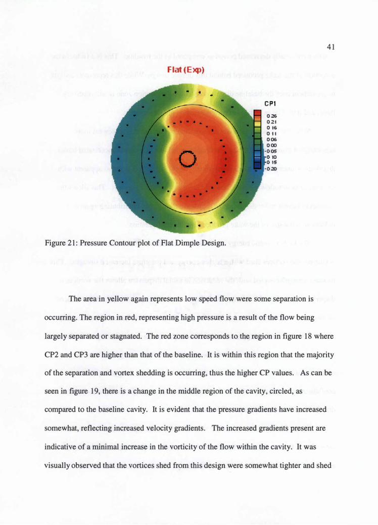
Figure 22 shows the size of the wake both from the top view and from a side
view. It can be seen from this figure that there is still a large amount of turbulence
associated with the flow that is leaving the cavity. The turbulence is somewhat
(a) (b) Figure 22: Improved flow attachment of the flat bottomed dimple.
43
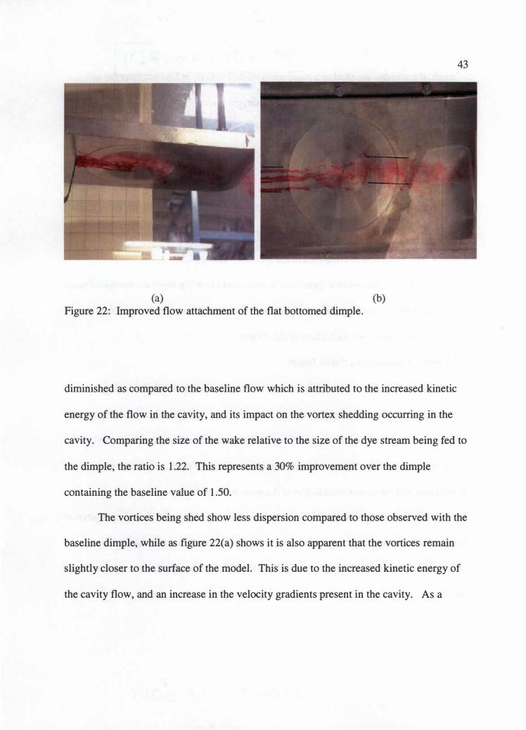
diminished as compared to the baseline flow which is attributed to the increased kinetic
energy of the flow in the cavity, and its impact on the vortex shedding occurring in the
cavity. Comparing the size of the wake relative to the size of the dye stream being fed to
the dimple, the ratio is 1.22. This represents a 30% improvement over the dimple
containing the baseline value of 1.50.
The vortices being shed show less dispersion compared to those observed with the
baseline dimple, while as figure 22(a) shows it is also apparent that the vortices remain
slightly closer to the surface of the model. This is due to the increased kinetic energy of
the cavity flow, and an increase in the velocity gradients present in the cavity. As a

44 result, the vortices are shed in a more concentrated pattern and do not disperse as
quickly. Note that while it is difficult to see from the photographs above, there is an
improvement in the flow attachment to the surface of the model as compared to the
baseline.
The portion of the flow attached to the surface remains so for a greater distance,
indicative of its increased energy. Measurements of the size of the wake in figure 22(b)
relative to the size of the dye stream show a ratio of approximately 1.22. This represents
a nearly 20% reduction as compared to the baseline value of 1.50.
While it is obvious that there is an improvement over the baseline, the turbulence
associated with this configuration is significant. Note that the vortices in the wake are
still a large distance from the surface of the dimple.
4-3 Dimple Containing a Small Insert
The next configuration tested is shown in figure 23 with detailed drawings in
Appendix A. In this design, an insert with a top diameter of 0.25 inches, reaching to 0.05
inches below the top level of the model surface and sloping at 45 degrees was employed.
It was hypothesized that this would show an improvement in terms of the pressure
distribution and the vortex shedding over the previous two designs.
The hoped improvement turned out to be the case. Figure 24 shows a snapshot of
the circulation taking place inside the cavity. Figure 24 (a) shows the majority of the
flow enters the cavity and turns inward as a result of flow attachment to the surface of the
insert.

45
Figure 23: The dimple configuration containing a small insert
46
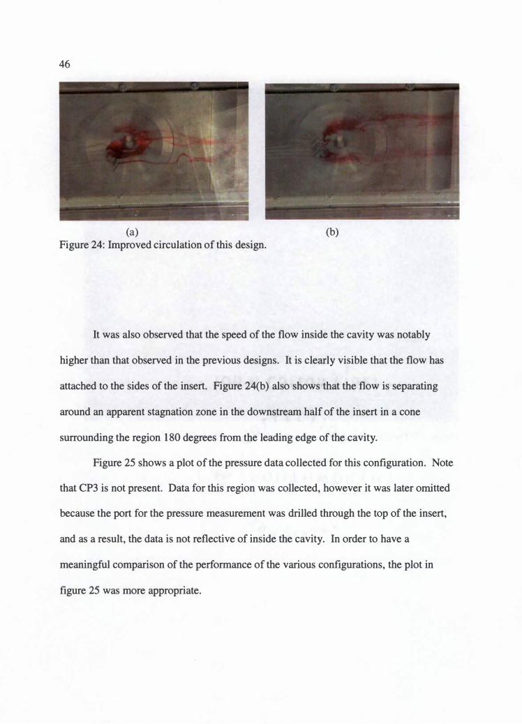
(a) (b) Figure 24: Improved circulation of this design.
It was also observed that the speed of the flow inside the cavity was notably
higher than that observed in the previous designs. It is clearly visible that the flow has
attached to the sides of the insert. Figure 24(b) also shows that the flow is separating
around an apparent stagnation zone in the downstream half of the insert in a cone
surrounding the region 180 degrees from the leading edge of the cavity.
Figure 25 shows a plot of the pressure data collected for this configuration. Note
that CP3 is not present. Data for this region was collected, however it was later omitted
because the port for the pressure measurement was drilled through the top of the insert,
and as a result, the data is not reflective of inside the cavity. In order to have a
meaningful comparison of the performance of the various configurations, the plot in
figure 25 was more appropriate.
47
0.35
0.3
0.25
0.2
0. 1 5
0 . 1
0.05
4 0
-0. 1 _,.__-------�------�---------'
Position (Degre e s)
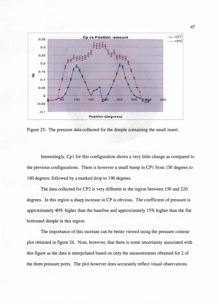
Figure 25: The pressure data collected for the dimple containing the small insert.
Interestingly, Cpl for this configuration shows a very little change as compared to
the previous configurations. There is however a small bump in CP 1 from 150 degrees to
180 degrees, followed by a marked drop to 190 degrees.
The data collected for CP2 is very different in the region between 150 and 220
degrees. In this region a sharp increase in CP is obvious. The coefficient of pressure is
approximately 40% higher than the baseline and approximately 15% higher than the flat
bottomed dimple in this region.
The importance of this increase can be better viewed using the pressure contour
plot obtained in figure 26. Note, however, that there is some uncertainty associated with
this figure as the data is interpolated based on only the measurements obtained for 2 of
the three pressure ports. The plot however does accurately reflect visual observations.

48
Sinai Mountain (Exp)
Figure 26: Pressure contour plot of dimple with small insert.
C P 1
0�
o.:u 0. 16
O. t t OJJ6 o.m
-o.os -0. 10 -o. ,�
- - ·0..20
Physically, the area in red between 150- 180 degrees corresponds to the region behind the
insert where the evidence of the stagnation zone was viewed using dye. Note first of all
that the red region, where the majority of vortex shedding is taking place is much more
concentrated than that of both the baseline dimple and the configuration of section 3-2.
This results in a decrease in the initial distribution pattern when the vortices are shed.
There is still some shedding occurring in the region in orange, and this can be seen in the
flow visualization runs. However, the majority of the vortex shedding is occurring in this
red region. As with the design of section 4-2, a less dispersed pattern of vortices upon
shedding is a contributing factor to the reduction in wake size behind the dimple.

49
Looking at the area circled in the center portion of figure 26, it is clearly
evident that there is an increase in the velocity gradients. The gradients in the X-Y plane
are greatly increased as can be seen by the changing in color from green to yellow and
red, representing decreasing velocity as the stagnation point is approached. The area in
green represents higher velocity circulation than was seen within the same region in the
designs of the previous sections. Not evident in this plot is that there is also an increase
in the gradient in the Z-direction. Attaching the flow to the surface of the insert also has
the effect of bringing the cavity flow closer to the main flow. While the velocities in
some regions are higher than the previous designs, the cavity flow here is much closer to
the main flow, thus the gradients in this direction are greatly increased.
The reason for the increased gradients is the insert. As the flow is drawn into the
cavity forward of the insert it is forced to attach to the insert. The flow must then
increase in speed as it travels around the surface of the insert in order to maintain
momentum 6• The flow eventually separates in the region denoted in red in figure 26
shedding a higher energy vortex in the region of the rear stagnation point of the insert.
The increase velocity due to flow attachment increases the velocity gradients in the
vicinity of the center of the cavity.
The increased velocity gradients concentrate the vorticity of this region of the
flow as per equation (1). From the video taken during the flow visualization, there is a
definite increase in the rate of vorticity production inside the cavity, indicative of the
increase in vorticity.
It should be noted at this point that the total amount of energy present in the
cavity does differ compared to that of the previous two designs. The cavity draws fluid

50 in from the main flow, which contains a given amount of energy, and the conservation
of energy law still applies. In the previous designs, this energy is dispersed over the
entire region of the dimple cavity, and thus the local velocities produced are low and the
gradients are low because the energy concentration is low. The effect of the insert is to
force the flow into a smaller area by having it attach to the insert. This concentrates the
available energy into a smaller region and thus locally increases the velocities and
gradients due to the increased energy concentration. Increasing the local kinetic energy is
the mechanism responsible for the results of his discussion.
Observations of the vortices shed from this design show that the individual
vortices are also smaller in size owing to the increased energy with which they are shed.
This is apparent from figure 27(b) which also shows that the vortices shed are much less
dispersed after they have left the cavity than the previous design. This is caused by the
increased energy with which the vortices are shed from the region in red of figure 26.
The decrease in dispersion results in a significantly reduced wake produced behind this
design compared to the previous designs as the flow interacts with it.
The decreased dispersion, and smaller size of the vortices shed are a result of their
improved energy concentration. Besides dispersing at a slower rate, the increased energy
of these vortices improves their strength. The improved strength improves their ability to
draw energy from the main flow resulting in a greater energy transport to the turbulent
boundary layer. This effect was readily apparent in the flow visualization. Figure 27(a)
shows both the reduced dispersion of the vortices traveling along the surface of the
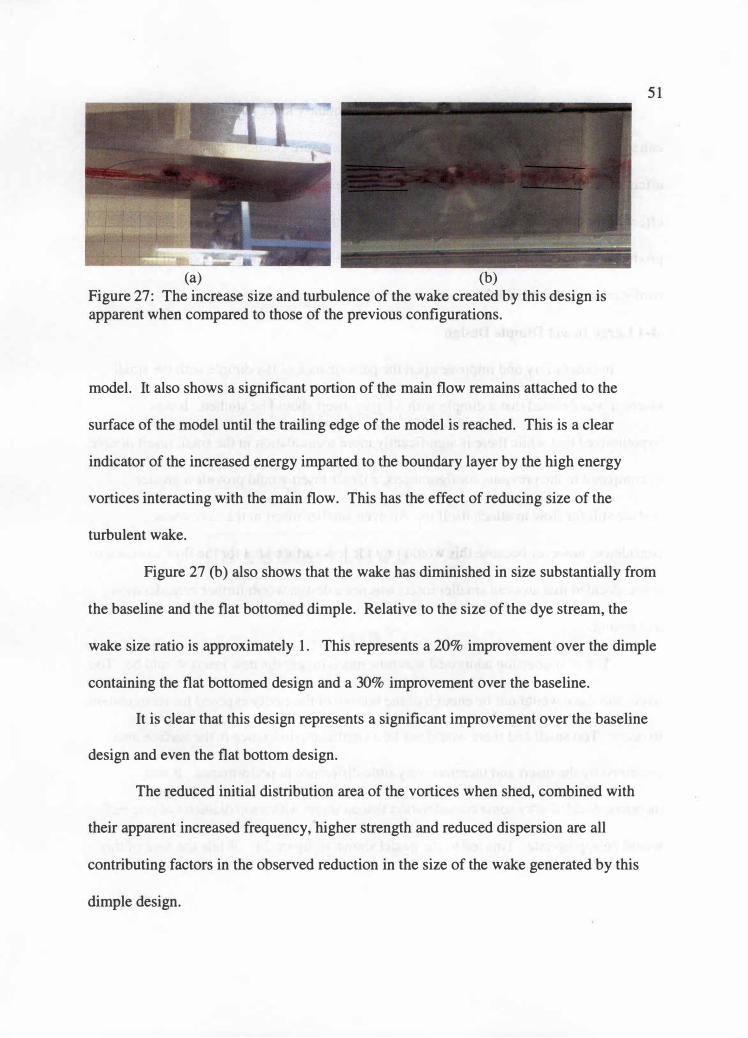
(a) (b) Figure 27: The increase size and turbulence of the wake created by this design is apparent when compared to those of the previous configurations.
model. It also shows a significant portion of the main flow remains attached to the
surface of the model until the trailing edge of the model is reached. This is a clear
indicator of the increased energy imparted to the boundary layer by the high energy
vortices interacting with the main flow. This has the effect of reducing size of the
turbulent wake.
5 1
Figure 27 (b) also shows that the wake has diminished in size substantially from
the baseline and the flat bottomed dimple. Relative to the size of the dye stream, the
wake size ratio is approximately 1. This represents a 20% improvement over the dimple
containing the flat bottomed design and a 30% improvement over the baseline.
It is clear that this design represents a significant improvement over the baseline
design and even the flat bottom design.
The reduced initial distribution area of the vortices when shed, combined with
their apparent increased frequency, higher strength and reduced dispersion are all
contributing factors in the observed reduction in the size of the wake generated by this
dimple design.

52
The increased energy imparted to the boundary layer flow past the cavity also
enhances the main flow's ability to resist adverse pressure gradients, and has the global
effect of reducing the size of the wake generated behind a golf ball in flight. The overall
effect of these improvements would be a significant reduction in the aerodynamic drag
produced by a golf ball in flight as compared to the baseline configuration and the
configuration of section 4-2.
4-4 Large Insert Dimple Design
In order to try and improve upon the performance of the dimple with the small
insert, it was decided that a dimple with a larger insert should be studied. It was
hypothesized that while there is significantly more recirculation in the small insert dimple
as compared to the previous configurations, a larger insert would provide a greater
surface still for flow to attach itself to. An even smaller insert in the cavity was
considered, however because this would provide less surface area for the flow to attach to
it was decided that an even smaller insert was not a design worth further consideration
and testing.
The next question addressed was how much bigger the new insert should be. Too
large, and there would not be enough of the bottom of the cavity exposed for recirculation
to occur. Too small and there would not be a significant difference in the surface area
presented by the insert and therefore very little difference in performance. It was
therefore decided after some consideration that an insert with a top diameter of one inch
would be appropriate. This led to the model shown in figure 28. While the base of this

53
Figure 28: Dimple with large cavity insert.
insert is much larger than that of the previous model, there is still a substantial portion of
the bottom of the cavity exposed and therefore available for recirculation.
Figure 29 shows the improvement in recirculation. In figure 29 (a), the dye has
been introduced into the cavity from upstream, off center of the insert. It can be seen in
the diagram that the flow has turned inward toward the flow attached to the insert. The
circulation is even more evident in figure 29(b ). This photograph was taken with the dye
rake placed inside the cavity, off center. The dye in figure 29(b) can be seen surrounding
the insert. It was visually observed that this happens quickly due to the speed with which
the circulating flow is moving.
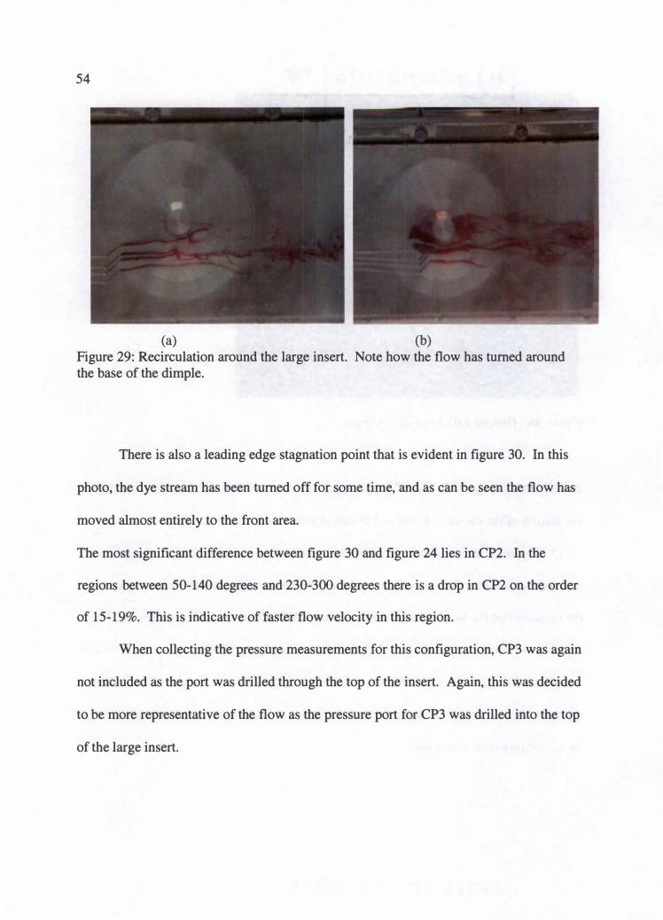
54
(a) (b) Figure 29: Recirculation around the large insert. Note how the flow has turned around the base of the dimple.
There is also a leading edge stagnation point that is evident in figure 30. In this
photo, the dye stream has been turned off for some time, and as can be seen the flow has
moved almost entirely to the front area.
The most significant difference between figure 30 and figure 24 lies in CP2. In the
regions between 50-140 degrees and 230-300 degrees there is a drop in CP2 on the order
of 15-19%. This is indicative of faster flow velocity in this region.
When collecting the pressure measurements for this configuration, CP3 was again
not included as the port was drilled through the top of the insert. Again, this was decided
to be more representative of the flow as the pressure port for CP3 was drilled into the top
of the large insert.

Figure 30: Evidence of the forward stagnation point.
Figure 3 1 is the plot obtained. Comparing it to the plot obtained for the dimple
containing the small insert, there are some observations to note. The first concerns the
plot for CPl .
55
It shows the same trend as all of the previous designs, including the small hump in
the area of 150 degrees that was observed for the cavity containing the small insert. The
difference here is that the hump is not as pronounced. The reason the hump exits in both
this case and the small insert design is likely due to vortex shedding occurring on the
surface of the insert in this region and thus the increase in pressure.
This is the area where the flow is attached to the side of the larger insert in this
configuration, and thus supports the visual observations that the flow in this region is
somewhat faster. The other difference between figures 30 and 24 is in the Peak CP
values. In figure 3 1 , it can be seen that the peak CP value occurs at approximately 180
degrees and has a value of approximately 0.32. This is an increase of nearly 10% over the
peak value in the dimple with the previous design. This is also in a very concentrated
area.

56
C P vs Position
� 2
0.4
0.35
0.3
0.25
0.2
e, 0. 1 5
0. 1
0.05
0
-0.05
-0. 1
Position ( De g rees)
Figure 3 1 : Pressure data obtained for the dimple containing a large insert.
The data in figure 3 1 was used to plot figure 32. Again a pressure coefficient
contour flood plot was obtained by interpolating the data used to produce figure 31 and
so it is subject to the same uncertainties as the other contour plots previously discussed.
The significant differences with this design can be seen in the area circled in the middle
of the contour plot of figure 32.
The green region represents lower pressures, and therefore much higher
velocities, comparable with the configuration of section 3-3 and much improved over the
designs of sections 4- 1 and 4-2.
The same information can be gleaned from this plot as was obtained from the
previous designs. The first observation deals with the region in red towards the rear enter

Big Mountai1 (E >q)) CP 1
0 .:» c .;: 1 0 . 16 0 , 1 1
I o o; 0 .00
� M -0 , 10
� . I t: -0 .33
Figure 32: Pressure contour plot of the dimple containing the large insert.
57
of figure 32. Notice how this region is much smaller in area than the design of section 4-
3. As discussed in previous sections, this is the region where the majority of the vortex
shedding is taking place.
This region being small in size means that as with the previous design, the initial
distribution pattern is more concentrated. In this case, this region is significantly reduced
in size as compared to the small insert design. As with the previous design, this is a
contributing factor in the reduction in the size of the wake produced behind this dimple
design.
It is also evident from figure 32 that the velocity gradients between the red area
and the green area within the circled region are very high as compared to all of the
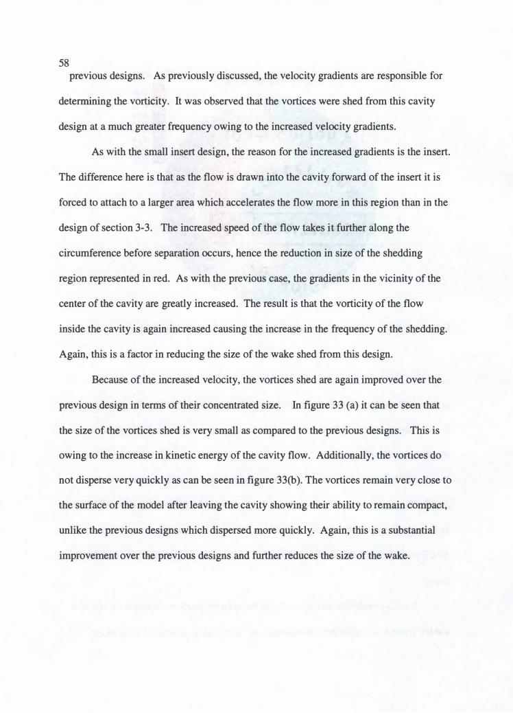
58 previous designs. As previously discussed, the velocity gradients are responsible for
determining the vorticity. It was observed that the vortices were shed from this cavity
design at a much greater frequency owing to the increased velocity gradients.
As with the small insert design, the reason for the increased gradients is the insert.
The difference here is that as the flow is drawn into the cavity forward of the insert it is
forced to attach to a larger area which accelerates the flow more in this region than in the
design of section 3-3. The increased speed of the flow takes it further along the
circumference before separation occurs, hence the reduction in size of the shedding
region represented in red. As with the previous case, the gradients in the vicinity of the
center of the cavity are greatly increased. The result is that the vorticity of the flow
inside the cavity is again increased causing the increase in the frequency of the shedding.
Again, this is a factor in reducing the size of the wake shed from this design.
Because of the increased velocity, the vortices shed are again improved over the
previous design in terms of their concentrated size. In figure 33 (a) it can be seen that
the size of the vortices shed is very small as compared to the previous designs. This is
owing to the increase in kinetic energy of the cavity flow. Additionally, the vortices do
not disperse very quickly as can be seen in figure 33(b). The vortices remain very close to
the surface of the model after leaving the cavity showing their ability to remain compact,
unlike the previous designs which dispersed more quickly. Again, this is a substantial
improvement over the previous designs and further reduces the size of the wake.

(a) (b)
59
Figure 33: The reduced wake and concentrated vortices shed from this design are much improved over the previous designs.
The increased kinetic energy also has the same effect as before in that the strength
of the vortices shed are much stronger. This enhances their ability to draw energy from
the main flow and pass it on to the boundary layer of the flow past the cavity. Again,
looking at figure 33(b) we see the result. There is a significant portion of the flow that
remains attached to the surface of the model until the end of the surface is reached.
Again, this is beneficial as it means that the flow has a greater ability to resist adverse
pressure gradients.
The combined effects of the higher energy cavity flow leads one to conclude that
there would be a reduction in the size of the wake as compared to the previous designs.
Comparing the size of the wake relative to the size of the dye stream being fed to the
dimple, the ratio is 0.60. This represents a 40% improvement over the dimple containing
the small insert, and a 50% decrease as compared to the flat configuration, and a 60%
improvement over the baseline. It can also be seen that the dye stream is influenced by

60 the large insert as it is getting spread apart as the flow is forced to travel along its
surface. As with the previous designs, the combined effects of the high energy,
concentrated strong vortices better able to impart energy to the main flow results in a
much reduced wake size behind this configuration. Additionally, this configuration is the
best of the four configurations tested. The reduction in wake, combined with the
increased ability of the flow to resist adverse pressure gradients results in the conclusion
that the aerodynamic drag produced behind a ball employing this configuration would be
significant as compared to the other three designs.
4-4-1 CFD Results
Figure 34 is a comparison of the results obtained experimentally on the left to that
obtained through the use of CFO. The two contour plots of the pressure distribution are
very similar. There is a difference in that the CFO code shows a forward stagnation
region that is not present in the experimental data.
Big Mountai1 (E,q,) CP I
0.:16 o.u
0.16 O.l t 0.116
0.00 ..,.., •Cl .IC
-0.15 ,OJIC)
Figure 34: The experimental Cp distribution compared to CFO results.
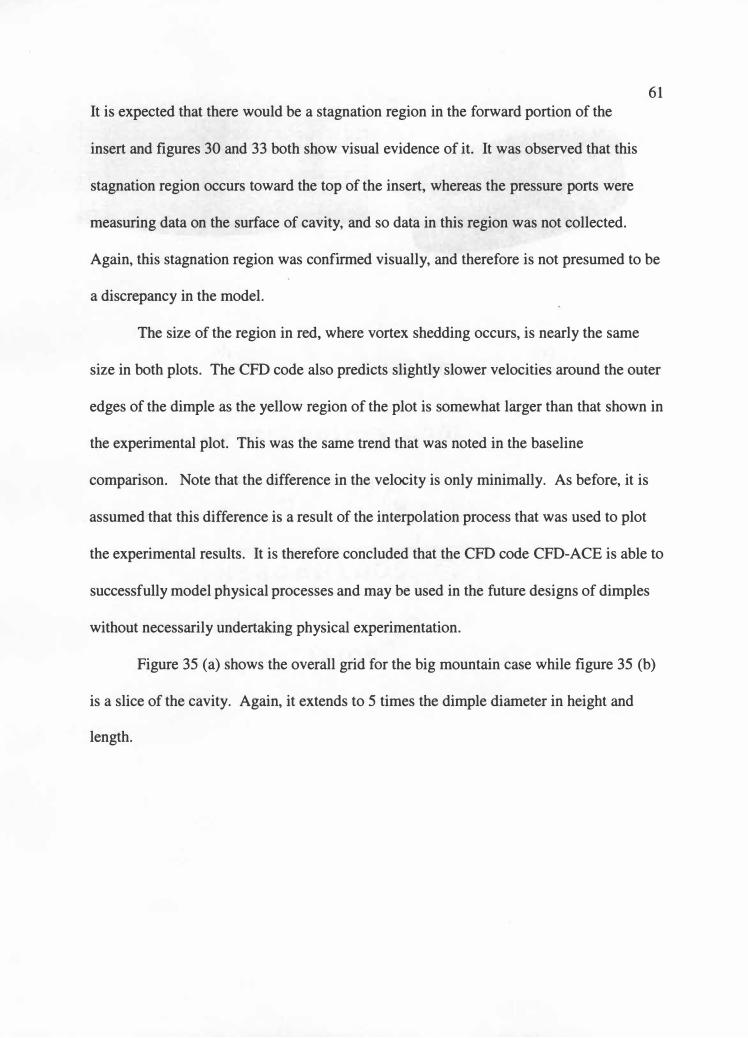
61 It is expected that there would be a stagnation region in the forward portion of the
insert and figures 30 and 33 both show visual evidence of it. It was observed that this
stagnation region occurs toward the top of the insert, whereas the pressure ports were
measuring data on the surface of cavity, and so data in this region was not collected.
Again, this stagnation region was confirmed visually, and therefore is not presumed to be
a discrepancy in the model.
The size of the region in red, where vortex shedding occurs, is nearly the same
size in both plots. The CFD code also predicts slightly slower velocities around the outer
edges of the dimple as the yellow region of the plot is somewhat larger than that shown in
the experimental plot. This was the same trend that was noted in the baseline
comparison. Note that the difference in the velocity is only minimally. As before, it is
assumed that this difference is a result of the interpolation process that was used to plot
the experimental results. It is therefore concluded that the CFD code CFD-ACE is able to
successfully model physical processes and may be used in the future designs of dimples
without necessarily undertaking physical experimentation.
Figure 35 (a) shows the overall grid for the big mountain case while figure 35 (b)
is a slice of the cavity. Again, it extends to 5 times the dimple diameter in height and
length.

62
(a) (b) Figure 35: The grid used for the CFD simulation.

63 Chapter 5
Conclusions and Recommendations
5-1 Concussions
In this study, the reduction in the size of the wake, and therefore the drag
produced, by a golf ball dimple was studied by means of increasing the strength of the
vortices shed within the dimple cavity. Through the use of flow visualization and
pressure distribution measurement, it was determined that an insert of sufficient size and
height installed in the cavity provided a means of increasing the strength of the vortices
shed by increasing the velocity gradients present within the cavity. The results were
compared to the computational fluid dynamics results from a commercial code CFD
ACE in order to validate its use in future work. The following conclusions were obtained:
1. The wake behind a golf ball dimple may be significantly reduced in size
through the strengthening of the vortices shed from within the dimple.
2. An effective way to increase the strength of the vortices shed is to have a large
insert within the cavity that provides a surface for circulating flow to attach to.
The resulting increase in velocity gradients provides the means through which
the vortex strength is improved.
3. The Stronger vortices draw energy from the main flow and impart that energy
to the boundary layer near the surface of the ball. This provides the boundary
layer more energy enabling it to remain attached longer, resulting in a reduced
wake.

64
4. CFD modeling reasonably simulates the cavity flow studied in this study. It
may be used with confidence in future, with care, and may be used to provide
details of the flow that can not be measured.
5-2 Recommendations
The following are recommendations for future work:
1. CFD may be used to explore dimple inserts of various sizes in order to
determine the effect of minimal changes.
2. More sophisticated testing is required to obtain a quantitative
estimate of the reduction in Co produced by the reduction in wake size.
And determine the interaction between successive dimples of the new
design developed here in order to determine an optimum distribution.
3. Test a scaled or full size golf ball to validate the results obtained in this
work.

65
References

66 References
1. http://observe.arc.nasa.gov/nasa/Tech Twice/Tech twice2.html
2. Kimura T and Tsutahara M, "Fluid Dynamic Effects of Grooves on Circular
Cylinder Surface", AIAA Journal, Vol.29, December 1991.
3. L.L Ting, "Effects of Dimple Size and Depth on Golf Ball Aerodynamic
Performance", FEDSM2003-45081, Proceedings of FEDSM'03 4th ASME_JSME
Joint Fluids Engineering Conference Honolulu, Hawaii, July 6-10, 2003.
4. L.L Ting, "Application of CFD Technology analyzing the Three Dimensional
Aerodynamic Behavior of Dimpled Golf Balls", IMEC2002-32349, Proceedings
of IMECE2002 ASME International Mechanical Engineering Congress &
Exposition, November 17-22, 2002, New Orleans, Louisiana.
5. Bearman, P.W., and Harvey, J.K., "Golf Ball Aerodynamics," Aeronautical
Quarterly, May 1976, pp. 1 12-122.
6. White F.M, "Viscous Fluid Flow", 2nd ed. McGraw-Hill, USA, 199 1 .
7. "Golf Balls, Slicing Through the Hype" Consumer Report Magazine, pp. 30-33,
May 2006
8. Rabinovich, S., "Measurement Errors: Theory and Practice", American Institute
of Physics, New York, 1995.
9. Saffman, P.G., "Vortex Dynamics", Cambridge University Press, 1997
10. Batchelor, G.K., "An introduction to Fluid Dynamics", Cambridge University
Press, New York, 1992.
11. Lugt, Hans, J., "An Introduction to Vortex Theory", Vortex Flow Press, Inc.,
1996.

67 12. Stephens, L.J., " Theory and Problems of Statistics", 3rd Ed., Schaum's Outline
Series, McGraw-Hill, Chicago, 1999.
13. WU, J.C, "Elements of Vorticity Dynamics", Tsinguhua University, Springer,
2006.
14. McDaniels, M.D., "Background and Theoretical Considerations For Utilizing
Water Tunnel Flow Visualization", Master's Dissertation, UTSI, 1996.
15. Aoyama Et al., United States Patent No. US 6,969,327, 29 Nov, 2005.
16. Ogg et al., United States Patent No. 6,979,272, 27 Dec, 2005.
17. United States Patent No. 6,979,271, 27 Dec., 2005.
18. Wilson Co, United States Patent No. 6,979,567, 10 Dec, 1996
19. Raymer, D.P., "Aircraft Design, an Experimental Approach", 3rd Ed., AIAA,
Virginia, 1999.
20. Karamcheti, K., "Principles of Ideal-Fluid Aerodynamics", Krieger Publishing
Company, Florida, 1980.
21. Vakili, A.D., University of Tennessee Space Institute, 2005-2006.
22. CFD-ACE Command Language Manual, Version 6.0, Feb. 2005.
23. Vector Launch Monitor, Operator's Manual, July, 2005
24. Golf Digest Magazine, July 2005.
25. Van Dyke, M. "An Album of Fluid Motion" Parabolic Press, California

68
Appendix A
Drawings
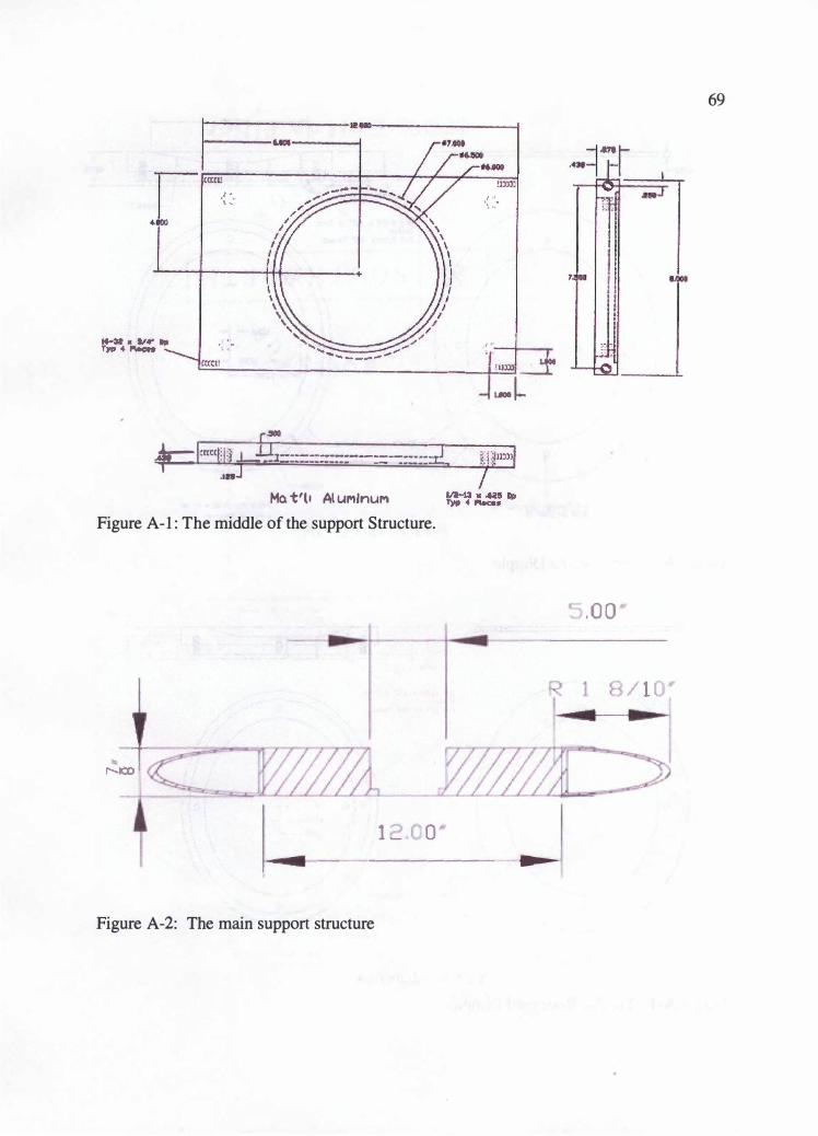
L..crr_ .. _t, ---------------�,1�1:m J
.Ar-l=vi� 1-¼-----------------::r.! ,--- ., __ ,.________ -- ----- ?
..• ] Mo. t'l• Al uMlnuM
Figure A-1: The middle of the support Structure.
1 _ 0
l.al �
---------·----
Figure A-2: The main support structure
69
. 0 0
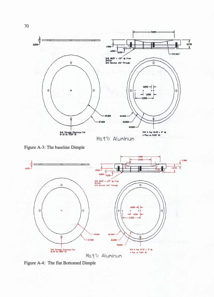
70
l i=:::I:z:c===:::::c::==:=::c::c::::::J
am,J
1 •
Ht 'Tlralol Cllortnct Far D-32 11n � IC
Figure A-3: The baseline Dimple
l c::::z:�====::::c::======n:c::::J OJZ50J
tA� .e.i' X .. 37• dp rl"Clfl
Drll 11.ltn:t .()40' TIToudl
Mo. t 'l : A luri inuM
Drtt Jl6a• x .437' � rro11 Bott011 Drtl Bo.lo.nc• .040' Tlro,qi
116.0000 16.5000
Jlrl\ .. 'tap 10-32 X Y � ,4 Pia on �.500' BC
Mo. t ' l : A lurri inurri Figure A-4: The flat Bottomed Dimple
·1
RI0.5667

l c:::::::::t::z:z=======�=========:::IJ:I::=:J O.!�J
Drf.l ,0625• X ,437• dp fro,, Botta,i :Ml BGlonc:1 .6-40' Tl'Y'olql
115,0000 116.5000
�.0000
Mo. t ' l : A luM inuM Figure A-5: The Small Insert Dimple
Drll &, � 10-32 X ,:!' � o4 Pies on :I.� BC
L756
71
0.(0)()
0,87�
1.7!51.
o .. s
0.11750
--------------------�----........ �---·
D--ll °'25' " .437' dp F"N>tl k>1to11 D-11 ll<Jo.nc:• .040' ThrD'9"
t,5,000) llb.SOOO
M n t ' l : A lu Minuri
Figure A-6: The Large Insert Dimple
0.2'51Xl--l I-• +
L��
n,-M ' .,ap 10-3t X ,!5' dp 4 Ra on s.st0• IIC

72 Vita
Captain Walter Robert Wilfred Michalchuk was born in Lachine, Quebec, Canada
on the 20th of January 1977. After graduating .from Vankleek Hill Colligate Institute in
June 1996 he joined the Canadian Armed Forces, completing Basic Officer T;aining in
Chilliwack, British Columbia in August of that year. He graduated from the Royal
Military College of Canada in May 2000 with a Bachelor Degree in Chemical and
Materials Engineering. As an Artillery Officer he was posted to the Combat Training
Center in Gagetown, New Brunswick where he served as an instructor until April 2001.
After transferring to the Canadian Air Force and graduating the Aerospace Engineering
Officer Basic Course in Borden Ontario in April 2002 he was posted to 416 Tactical
Fighter Squadron in Cold Lake, Alberta where he served as the Aircraft Production
Officer until July 2004. In August 2004 he began graduate studies at the University of
Tennessee Space Institute, completing all the requirements for the degree of Master of
Science, Aerospace Engineering in August 2006. Upon completion he is posted to
National Defense Headquarters in Ottawa, Ontario where he will serve with the
Directorate of Aerospace Engineering Support. In his spare time he is an avid golfer,
archer and musician. He is married to Captain Georgia Dryden of Peterborough, Ontario.
5873 8921t 18 : ,.. ,... ,.., � "''"'"' UR iit'I