
AN INVESTIGATION INTO COMBINING BOTH FACIAL DETECTION …eprints.lincoln.ac.uk/26652/1/McDonagh,...
83
AN INVESTIGATION INTO COMBINING BOTH FACIAL DETECTION AND LANDMARK LOCALISATION INTO A UNIFIED PROCEDURE USING GPU COMPUTING J M McDonagh MSc by Research 2016
Transcript of AN INVESTIGATION INTO COMBINING BOTH FACIAL DETECTION …eprints.lincoln.ac.uk/26652/1/McDonagh,...
AN INVESTIGATION INTO COMBINING BOTH FACIAL DETECTION AND
LANDMARK LOCALISATION INTO A UNIFIED PROCEDURE USING GPU
COMPUTING
J M McDonagh
MSc by Research
2016

AN INVESTIGATION INTO COMBINING BOTH FACIAL DETECTION AND LANDMARK LOCALISATION INTO A UNIFIED PROCEDURE
USING GPU COMPUTING

MCD11211426 John McDonagh iii
Acknowledgements
Many thanks to my supervisor Georgios Tzimiropoulos for your guidance and
support throughout the course of this project.

MCD11211426 John McDonagh iv
Abstract
This thesis describes the design and implementation of a unified framework for face
detection and landmark alignment in arbitrary in the wild images. Traditionally, both of
these problems have been addressed separately in literature with impressive results
being recently reported in both of these fields. But, if one was to construct a pipeline
consisting of a state-of-the-art face detection method followed by a state-of-the-art
facial landmark localisation algorithm, the overall performance outcome would not be
proficient enough to be used in high level algorithms such as face recognition and
facial expression. This is because the accuracy produced by the face detector is not
sufficiently high enough to initialise the landmark localisation algorithm.
To address this aforementioned limitation, this thesis aims to propose an approach
that combines both of these tasks into a single unified algorithm that can be run in real
time, by utilising the parallel computing architecture of the graphics processing unit
(GPU). This will be done by using a Cascaded-Regression (CR) algorithm in a sliding
window fashion. The proposed system will exploit the CR algorithms ability to compute
the 2D pose of a face from rough initial estimates, in order to generate a Hough-
Transform voting scheme for detecting candidate faces and filtering out irrelevant
background. The obtained detection surface will then be further refined using SVM to
yield both face detections and the location of their parts.
The proposed system for this thesis will be built within the MATLAB environment, using
a MEX-file which will provide an interface to the proposed CUDA algorithm. The results
of which, will be tested against current state-of-the-art methods for both face detection
and landmark localisation.
We evaluate performance on the most widely used data sets in face detection, namely
annotated faces in-the-wild (AFW) (Zhu and Ramanan, 2012), Face Detection Dataset
and Benchmark (FDDB) (Jain and Learned-Miller, 2010) and Caltech Occluded Faces
in the Wild (COFW) (Burgos-Artizzu, Perona and Dollár, 2013). The empirical results
demonstrate that the proposed unified framework achieves state-of-the-art
performance in both face detection and facial alignment, and that our detector clearly
outperforms all commercial and published methods by a margin of over 10% in
detection accuracy on the AFW dataset.

MCD11211426 John McDonagh v
Table of Contents
1 Introduction ....................................................................................................... 1
1.1 Aims .............................................................................................................. 4
2 Related Work ..................................................................................................... 6
2.1 Face Detection .............................................................................................. 6
2.2 Facial landmark localisation .......................................................................... 8
3 SIFT .................................................................................................................. 11
3.1 Keypoint Descriptor ..................................................................................... 11
4 Deformable Global Consensus Model ........................................................... 14
4.1 Shape model and appearance .................................................................... 14
4.1.1 Shape model ........................................................................................ 14
4.1.2 Appearance .......................................................................................... 17
4.2 Deformable model fitting with PO-CR ......................................................... 18
4.3 Training ....................................................................................................... 22
4.4 Hough-Transform Voting ............................................................................. 22
4.5 Final re-scoring ........................................................................................... 23
4.6 Complexity .................................................................................................. 23
5 CUDA ................................................................................................................ 24
5.1 CUDA architecture ...................................................................................... 24
5.1.1 Streaming multiprocessor (SMX) .......................................................... 25
5.2 Compute Capability ..................................................................................... 26
5.3 Kernel Functions ......................................................................................... 26
5.4 Thread hierarchy ......................................................................................... 27
5.4.1 Thread Blocks ....................................................................................... 28
5.4.2 Threads ................................................................................................ 29
5.5 Memory Hierarchy ....................................................................................... 29
6 Implementation ................................................................................................ 32
MCD11211426 John McDonagh vi
6.1 DGCM ......................................................................................................... 34
6.1.1 Memory allocation ................................................................................ 34
6.1.2 SIFT ...................................................................................................... 34
6.1.3 PO-CR .................................................................................................. 35
6.1.4 CUDA Vector-Matrix multiplication ....................................................... 36
6.1.5 Voting ................................................................................................... 38
6.2 Support Vector Machine (SVM) ................................................................... 42
6.2.1 Feature normalisation ........................................................................... 43
6.2.2 Cross-validation .................................................................................... 43
6.2.3 Training ................................................................................................. 44
6.2.4 Classification ........................................................................................ 44
7 Results ............................................................................................................. 46
7.1 Performance measures ............................................................................... 46
7.2 Face detection ............................................................................................. 47
7.2.1 Annotated faces in-the-wild .................................................................. 47
7.2.2 Face Detection Dataset and Benchmark .............................................. 49
7.3 Landmark localisation ................................................................................. 50
7.4 Execution times ........................................................................................... 52
7.5 Images ........................................................................................................ 53
7.5.1 AFW...................................................................................................... 53
7.5.2 FDDB .................................................................................................... 55
7.5.3 COFW ................................................................................................... 58
8 Conclusion....................................................................................................... 60
9 Reference ......................................................................................................... 61
10 Appendix A ...................................................................................................... 67
10.1 CUDA and OpenCL Performance comparison ........................................ 68
10.2 Conclusion ............................................................................................... 73

MCD11211426 John McDonagh vii
List of Figures
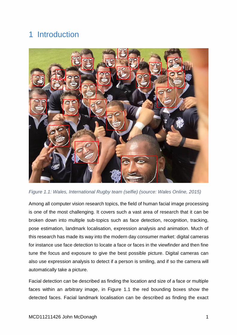
Figure 1.1: Wales, International Rugby team (selfie) (source: Wales Online, 2015) .. 1
Figure 1.2: An example of face detection using the Deformable Part Model (DPM)
(Mathias et al, 2014). Using the PASCAL VOC protocol of 50% overlap (Everingham,
et al., 2009), we can see that the woman on the left, although detected, does not
pass the standard detection protocol. Red bounding boxes are the ground truth,
yellow boxes are detected faces and green boxes are false positives. ...................... 2
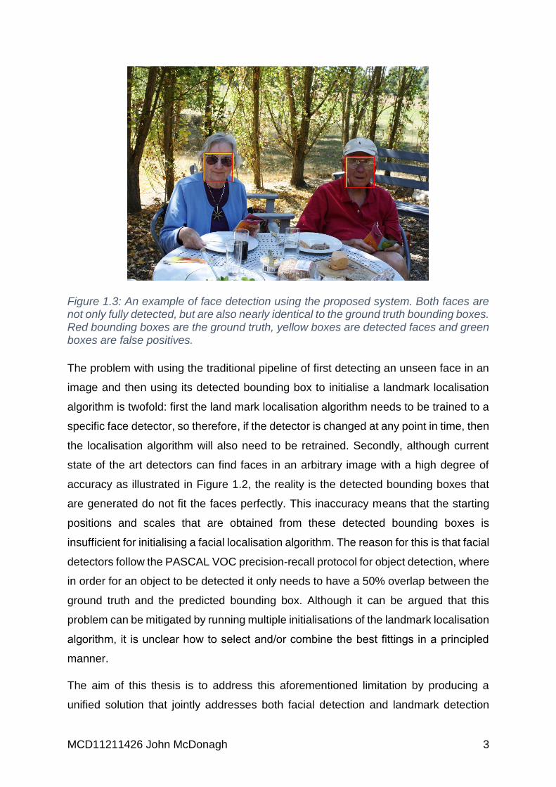
Figure 1.3: An example of face detection using the proposed system. Both faces are
not only fully detected, but are also nearly identical to the ground truth bounding
boxes. Red bounding boxes are the ground truth, yellow boxes are detected faces
and green boxes are false positives. .......................................................................... 3
Figure 1.4: Examples of detected faces from the AFW dataset using the standard
PASCAL VOC protocol of 50% overlap. Red bounding boxes are the ground truth
and yellow boxes are detected faces. ........................................................................ 4
Figure 3.1: For each 4x4 sub-region, the gradient magnitudes are weighted with the
Gaussian filter (blue circle), the result of which is then added to the corresponding
bin of the sub-region histogram that matches the gradient orientation. (Source: Gil,
2013) ........................................................................................................................ 12
Figure 4.1: Examples of annotated landmarks for both frontal and profile faces from
the Helen and ALFW datasets ................................................................................. 15
Figure 4.2: frontal and profile mean shapes ............................................................. 16
Figure 4.3: Statistical distribution of facial feature points. The black dots represent
600 facial shapes that have been normalised by Procrustes analysis. The red dots
signify the mean shape. (Wang et.al, 2014) ............................................................. 17
Figure 4.4: Example of a face warped to the mean shape. The left image is the
source image taken from a training set with the landmarks triangulated using
Delaunay triangulation, the pixels within each triangle are then warped to the
corresponding triangle in the mean shape. This gives us the shape-free texture,
which is shown in the right image ............................................................................. 18

MCD11211426 John McDonagh viii
Figure 4.5: Overview of the proposed Deformable Global Consensus Model. For
each iteration, if the current threshold is above zero, Hough-Transform voting is used
to reject any shapes peaks below the threshold. ...................................................... 21
Figure 5.1: Kepler GK110 Full chip block diagram (Source: NVIDIA, 2012, p6) ....... 24
Figure 5.2: SMX: 192 single‐precision CUDA cores, 64 double‐precision units, 32
special function units (SFU), and 32 load/store units (Source: NVIDIA, 2012, p8) ... 25
Figure 5.3: Thread hierarchy in the CUDA programming model. (Source: NVIDIA,
developer zone, 2015) .............................................................................................. 28
Figure 5.4: Kepler’s memory hierarchy (Source: NVIDIA, 2012, p13) ...................... 30
Figure 6.1: System overview, the red outlined boxes are the Mex functions that are
used to provide an interface to CUDA C++ .............................................................. 32
Figure 6.2: 2D matrix allocation. When allocating device memory via the
cudaMallocPitch function call, rows are padded (yellow blocks) to guarantee that the
beginning of each row begins on a 128 memory boundary. ..................................... 34
Figure 6.3: Warp reduction using shuffle down, for illustrative purposes this figure
only shows a half warp (16 lanes). The first parameter of the __shfl_down intrinsic is
the register to return, the second is the offset from the calling lane of the warp and
the third parameter is the width of the warp segment which must be of size 2, 4, 8,
16, or 32. The default size is 32. .............................................................................. 37
Figure 6.4: Original image from the AFW dataset .................................................... 38
Figure 6.5: Hough-Transform voting surface after first iteration ............................... 39
Figure 6.6: Hough-Transform voting surface after second iteration ......................... 39
Figure 6.7: Hough-Transform voting surface after fifth iteration ............................... 39
Figure 6.8: Hough-Transform voting surface after tenth iteration ............................. 40
Figure 6.9: Hough-Transform voting surface after fifteenth iteration ........................ 40
Figure 6.10: SVM scores generated for candidate faces .......................................... 40
Figure 6.11: Final fitted results after threshold has been applied ............................. 41
Figure 6.13: Stream compaction. Any vote score (yellow boxes) with a value equal or
less than one is set to minus one in the index array, then the function copy_if from
the thrust library is used to compact the array. ......................................................... 41
Figure 6.14: Optimal separating hyperplane, the three filled in shapes are the
support vectors (Source: OpenCV, 2016) ................................................................ 42
Figure 7.1: Precision-Recall curve of different evaluation methods on the AFW
dataset. With Intersection-over-Union (IoU) overlap set to 50% ............................... 48

MCD11211426 John McDonagh ix
Figure 7.2: Precision-Recall curve of different evaluation methods on the AFW
dataset. With Intersection-over-Union (IoU) overlap set to 75% ............................... 48
Figure 7.3: FDDB Discrete scores. ........................................................................... 49
Figure 7.4: FDDB Continuous scores (true positive ratio is IoU between detection
ellipse and ground-truth ellipse.) .............................................................................. 50
Figure 7.5: Accumulated point-to-point error, relative to size of face, for 474
annotated faces from the AFW dataset. ................................................................... 51
Figure 7.6: Accumulated point-to-point error, relative to size of face, for 507
annotated faces from the COFW dataset. ................................................................ 51
Figure 8.1: FDDB dataset. Example of low resolution missed faces. Yellow ellipses
show faces that are detected, and red ellipses show faces that are not detected .... 60
Figure 10.1: Unified performance comparison of selected benchmarks using
NVIDIA’s GeForce GTX 280 and GTX480. It is assumed that CUDA and OpenCL
have a similar performance if the result lies between 0.9 and 1.1 (Source: fang et al,
2011) ........................................................................................................................ 70
Figure 10.2: Initial benchmarks for CUDA and OpenCL, running near identical kernel
code on an NVIDIA Tesla C1060 GPU. (Source: Komatsu et al. 2010) ................... 72
Figure 10.3: Performance of benchmarks after applying manual optimisations.
(Source: Komatsu et al. 2010) .................................................................................. 72

MCD11211426 John McDonagh x
List of Tables
Table 5.1: CUDA Compute Capability ...................................................................... 26
Table 7.1: Scaling factors and resulting grid dimensions of a VGA image, with
execution times for frontal, right profile and left profile models measured in
milliseconds .............................................................................................................. 52
Table 10.1: Discrete graphics chip market share 2015 (Source: Jon Peddie
Research, 2015) ....................................................................................................... 67
Table 10.2: CUDA and OpenCL GPU kernel execution, data transfer and application
running costs. All times are measured in seconds (Source: Karimi et al, 2010). ...... 69
Table 10.3: CUDA and OpenCL execution times for a tiled 3D-FWT implementation
on an input video containing 64 frames of increasing sizes. All times are measured in
milliseconds. (Source: Bernabé et al, 2012). ............................................................ 71
MCD11211426 John McDonagh 1
1 Introduction
Figure 1.1: Wales, International Rugby team (selfie) (source: Wales Online, 2015)
Among all computer vision research topics, the field of human facial image processing
is one of the most challenging. It covers such a vast area of research that it can be
broken down into multiple sub-topics such as face detection, recognition, tracking,
pose estimation, landmark localisation, expression analysis and animation. Much of
this research has made its way into the modern day consumer market: digital cameras
for instance use face detection to locate a face or faces in the viewfinder and then fine
tune the focus and exposure to give the best possible picture. Digital cameras can
also use expression analysis to detect if a person is smiling, and if so the camera will
automatically take a picture.
Facial detection can be described as finding the location and size of a face or multiple
faces within an arbitrary image, in Figure 1.1 the red bounding boxes show the
detected faces. Facial landmark localisation can be described as finding the exact

MCD11211426 John McDonagh 2
location of facial features, such as eyes, lips, nose, jawline etc., in Figure 1.1 these
are shown as the white facial shapes.
Facial detection and landmark localisation are both non-trivial problems. This is due
to the human face being a highly variable, deformable object that can vary drastically
from image to image, due to pose (scale, rotation and translation), expression, identity,
occlusion and illumination. Research into solving both detection and localisation has
traditionally been approached as two separate problems with numerous research
papers in each field reporting extremely good results for very challenging in-the-wild
images. However, for many subsequent, higher level tasks, like face recognition, facial
expression and attribute analysis, what matters most is the overall performance in
terms of accuracy in landmark localisation. Notably, recent state-of-the-art methods
for such tasks rely heavily on the accurate detection of facial landmarks, see for
example Chew, et al. (2012) and Chen, et al. (2013).
Figure 1.2: An example of face detection using the Deformable Part Model (DPM) (Mathias et al, 2014). Using the PASCAL VOC protocol of 50% overlap (Everingham, et al., 2009), we can see that the woman on the left, although detected, does not pass the standard detection protocol. Red bounding boxes are the ground truth, yellow boxes are detected faces and green boxes are false positives.
MCD11211426 John McDonagh 3
Figure 1.3: An example of face detection using the proposed system. Both faces are not only fully detected, but are also nearly identical to the ground truth bounding boxes. Red bounding boxes are the ground truth, yellow boxes are detected faces and green boxes are false positives.
The problem with using the traditional pipeline of first detecting an unseen face in an
image and then using its detected bounding box to initialise a landmark localisation
algorithm is twofold: first the land mark localisation algorithm needs to be trained to a
specific face detector, so therefore, if the detector is changed at any point in time, then
the localisation algorithm will also need to be retrained. Secondly, although current
state of the art detectors can find faces in an arbitrary image with a high degree of
accuracy as illustrated in Figure 1.2, the reality is the detected bounding boxes that
are generated do not fit the faces perfectly. This inaccuracy means that the starting
positions and scales that are obtained from these detected bounding boxes is
insufficient for initialising a facial localisation algorithm. The reason for this is that facial
detectors follow the PASCAL VOC precision-recall protocol for object detection, where
in order for an object to be detected it only needs to have a 50% overlap between the
ground truth and the predicted bounding box. Although it can be argued that this
problem can be mitigated by running multiple initialisations of the landmark localisation
algorithm, it is unclear how to select and/or combine the best fittings in a principled
manner.
The aim of this thesis is to address this aforementioned limitation by producing a
unified solution that jointly addresses both facial detection and landmark detection

MCD11211426 John McDonagh 4
while at the same time producing a high degree of accuracy in landmark localisation.
The proposed approach that is used in this thesis is largely motivated by the efficiency
and robustness of recent Cascaded Regression (CR) approaches in facial landmark
localisation. Instead of using a face detector to initialise them, the system that is
proposed in this thesis, will instead, employ them in a sliding window fashion, in order
to detect the location of all faces in an image.
This will be accomplished in real time by utilising the parallel computing architecture
of the graphics processing unit (GPU), and the implementation will be based on using
NVIDIAs Compute Unified Device Architecture (CUDA). The proposed system will be
built within the MATLAB environment, using a MEX-file that will provide the interface
to CUDA. The results of which, will be tested against current state-of-the-art methods
for both face detection and landmark localisation.
1.1 Aims
Figure 1.4: Examples of detected faces from the AFW dataset using the standard PASCAL VOC protocol of 50% overlap. Red bounding boxes are the ground truth and yellow boxes are detected faces.
As can be seen from Figure 1.4 having an overlap threshold of 50% to detect a face
can produce a wide degree of inaccuracy in the actual detection of a face. The aim of
this thesis is to propose a unified solution that jointly addresses both facial detection
and landmark detection to not just find faces in an arbitrary image but to detect them
with a high degree of accuracy. This will be achieved by exploiting the ability of the
Cascaded-Regression algorithm PO-CR (Tzimiropoulos, 2015) to compute the 2D

MCD11211426 John McDonagh 5
pose of a face from rough initial estimates over a grid which covers the entire image,
to generate peaks via a Hough-transform voting scheme to find the position of faces
in an image. Thereby if a face is detected, it will be able to generate a bounding box
from the final pose estimation, that is close to the ground truth bounding box.

MCD11211426 John McDonagh 6
2 Related Work
2.1 Face Detection
Ever since the ground-breaking work of Viola and Jones (2004), the topic of face
detection has become one of the most actively researched areas within the computer
vision community. The results of their work can also be seen in many of today’s high-
tech commercial gadgets, such as digital cameras and smartphones.
The objective of face detection is to localise and determine the scales of all faces that
are contained within an arbitrary image. This is not a trivial problem to solve, due to
variations in pose, illumination, expression and occlusion. In recent years a multitude
of different methodologies into the problem of solving multi-view face detection have
been proposed, which have reported a varying degree of success. These
methodologies can be summarised into three distinct groups, cascade, deformable
part models (DPM) and Neural Networks.
The Viola and Jones (2001) detector, which is also called the detector cascade, made
it possible to rapidly detect up-right faces in real-time with very low computational
complexity. Their detector was successful because of three reasons: firstly, they
represented grey scale images in a structure which they called the integral image; this
allowed Haar-like features to be calculated extremely fast. Secondly, simple classifiers
where generated by selecting a small number of critical features from a larger set of
potential features using the adaptive boosting algorithm (AdaBoost) (Freund and
Schapire, 1995). Finally, to improve the speed of the detector, each search window is
initially checked against a simple classifier, if the search window passes that stages
threshold value, it would then become subject to more rigorous testing against more
complex classifiers. This threshold culling is repeated at each stage in the cascade,
enabling background regions in the image to be discarded as quickly as possible, with
little computation.
While Viola and Jones (2001) detector could accurately find up-right faces of any scale
in an arbitrary image, they often failed to detect faces with arbitrary poses or that were
partially occluded. To address the issue of non-upright and non-frontal faces, Viola
and Jones (2003) proposed a two stage approach, which first estimates the pose of

MCD11211426 John McDonagh 7
the face with the use of a decision tree, and then uses the corresponding cascade
detector that is trained on that pose. The problem with using this method is that any
errors made while evaluating the pose in the decision tree are irreversible.
Instead of making an exclusive selection of the path for a sample, Huang, et al. (2005)
multi-view vector boosting algorithm used a width first search (WFS) tree structure,
where each branching node computes a vector, this allowed the sample to be passed
into multiple children. By using this soft branching technique, the risk of
misclassification is greatly reduced compared to Viola and Jones (2003) decision tree
method. Huang, et al. (2005) multi-view face detector covers an in-plane rotation of
±45 degrees. To make it rotation invariant they simply constructed 3 more detectors
at 90, 180 and 270 degrees.
Most of the recent research into face detectors is based on the DPM structure which
was originally proposed by (Felzenszwalb, et al., 2008), where a face is defined as a
collection of parts. These parts are defined via unsupervised or supervised training,
and a classifier, the so-called latent SVM, is trained to find those parts and their
geometric relationship. They are usually fine-tuned to work efficiently with Histogram
of Orientation (HOG) features.
A unified approach to face detection, pose estimation and landmark (eyes, eyebrows,
nose mount and jaw line) localisation using the DPM framework was proposed by (Zhu
and Ramanan, 2012). Their approach defined a part at each facial landmark and used
a mixture of tree based structure models to capture the topological changes due to
varying viewpoints.
DMP detectors are robust to partial occlusion because they can detect faces even
when some of the parts are not present. A notable extension to (Zhu and Ramanan,
2012) which handles occlusion of parts in a more robust way was suggested by (Ghiasi
and Fowlkes, 2014) where they describe a hierarchical DPM for face detection and
landmark localisation that explicitly models likely patterns of occlusion and improves
landmark localisation. Their model can also predict which landmarks are occluded.
Mathias, et al. (2014) reported in their paper that a properly tuned vanilla DPM face
detector performs comparably with a multi-channel, multi-view version of the Viola-
Jones detector, and that they both produce state-of-the-art performance on both the
FDDB and AFW data sets. Therefore, it can be argued that part based approaches
MCD11211426 John McDonagh 8
are not always superior to standard approaches based on multi-view rigid templates,
especially when a large amount of training data is available.
Observing that aligned face shapes provide better features for face classification,
(Chen, et al., 2014) proposed to combine face detection and alignment into the same
cascade framework by learning a classifier at each stage, not only on the image, but
also on the previous stages estimated shape, in what is called shape-indexed features.
Chen, et al. (2014) along with Mathias, et al. (2014) are the current state of-the-art in
face detection.
2.2 Facial landmark localisation
Finding facial landmarks such as eyes, nose, mouth and chin in arbitrary images is not
a trivial task. This is due to the subjective morphology of the human face. Human
faces, even of the same person can vary enormously from image to image, due to
pose, illumination, occlusion and expression. The human face is typically modelled as
a deformable object that can vary in terms of shape and appearance. Having accurate
facial alignment is essential for many higher level applications such as face
recognition, tracking, animation and expression analysis.
In computer vision there has been a long history in the field of face alignment, where
numerous approaches such as Active Shape Models (ASM) (Cootes & Taylor, 1992),
Active Appearance Models (AAM) (Cootes & Taylor, 1992; Cootes, et al., 2001;
Matthews and Barker, 2004), Constrained Local Models (CLM) (Cristinacce and
Cootes, 2006; Saragih, et al., 2011) and most recently cascaded regression-based
techniques (CR) have been proposed to solve this conundrum, with varying degrees
of success (Dollar, et al., 2010; Cao, et al., 2012; Tzimiropoulos, 2015).
One of the earliest works in facial alignment was the ASM which was originally
proposed by (Cootes & Taylor, 1992). ASMs use a point distribution model (PDM) to
capture the variations in shape from a training set of images. The PDM is learned off-
line by first applying Procrustes analysis and then Principle Component Analysis
(PCA).
A natural successor to ASMs was the AAM which was first suggested by (Cootes, et
al., 1998). AAMs try to solve the problem of face alignment by capturing the combined
statistical variations of both shape and texture into a single appearance model using
MCD11211426 John McDonagh 9
linear regression. A more optimised approach of matching statistical models of
appearance to images was proposed by (Cootes, et al., 2001), which replaced the
linear regression model with a more simplified Gauss-Newton gradient descent
procedure. They assumed that because the Jacobian matrix was being computed in
a normalised reference frame, it could be considered approximately fixed and thus
could be pre-calculated by numerical differentiation from the training set. This was
later showed to perform badly, both in terms of the number of iterations required to
converge and in the accuracy of the final fit (Matthews and Barker, 2004).
To avoid the resulting inefficiencies in convergence and robustness during fitting, the
inverse compositional algorithm (ICA) was proposed by (Matthews and Barker, 2004).
But, unlike the previous AAMs that jointly built generative models of both texture and
shape, ICA treated the variations of shape and appearance independently. ICA is
based on a variation of the Lucas-Kanade (LK) image alignment algorithm (Lucas and
Kanade, 1981), which is a Gauss-Newton gradient descent non-linear optimisation
algorithm.
The problem with the LK algorithm is that it is extremely computationally intensive. The
reason for this is, because the appearance parameters vary with each iteration and
hence the Jacobian, the Hessian and its inverse need to also be recalculated. ICA
solves this problem by reversing the roles of the reference and template images, as
suggested by (Hager and Belhumeur, 1998), therefore making it possible to pre-
calculate the Jacobian and the inverse Hessian matrix. Because ICA reverses the
roles of the reference and template images, the update parameters need to be inverted
before they are composed with the current estimate of the warp parameters. This lead
to a very efficient fitting algorithm, which achieved faster convergence and enhanced
convergence properties compared to previous AAMs.
However, this was later shown to not work very well on unseen images, because the
learned appearance model had limited expressive power in capturing variations in
pose, expression, and illumination (Cristinacce and Cootes, 2006). AAMs were also
shown to be very sensitive to initialisation because of the gradient descent
optimisation. (Asthana, et al., 2009)
Because of the inability of AAMs to generalise well to unseen images, recent research
has been in the use of CLMs which was introduced by (Cristinacce and Cootes, 2006).

MCD11211426 John McDonagh 10
CLMs are based on ASMs, and use a similar appearance model to AAMs, but instead
of trying to approximate the image pixels directly, they sample texture patches around
the individual feature points. CLMs have been shown to be more robust to occlusion
and illumination compared to AAMs, and they also outperform AAMs in terms of
landmark accuracy. A notable extension to CLM is in the seminal work of (Saragih, et
al., 2011), where they proposed a framework for deformable model fitting, known as
the Regularized Landmark Mean-Shift (RLMS), which has shown state-of-the-art
results under uncontrolled natural settings.
The proposed system in this thesis uses cascade regression (CR) to fit a deformable
template to each sub-window in a given image. CR is based on Cascade pose
regression (CPR) which was originally proposed by (Dollar, Welinder and Perona,
2010). CPR is an iterative regression method that uses the pose estimation from the
previous regressor in the cascade to calculate the new shape-index features, which
are to be used as input to the current regressor. Starting from the mean shape the
pose estimation is gradually refined with each step in the cascade. CPR has been
shown to produce exceptional results on a variety of tasks and, owing to its efficiency
and accuracy, it has recently been the focus of investigation by numerous authors for
the problem of face alignment.
The idea of using CPR within the field of face alignment was first explored by (Cao, et
al., 2012) where they used Explicit Shape Regression (ESR) for facial alignment. Their
approach produced exceptional results in terms of both accuracy and efficiency on the
Labelled Face Parts in the Wild (LFPW) data set (Belhumeur, et al., 2011).
Project-Out Cascaded Regression (PO-CR) proposed by (Tzimiropoulos, 2015) uses
regression to learn and employ a sequence of averaged Jacobian and Hessian
matrices, one for each iteration, in a subspace orthogonal to the facial appearance
variation. PO-CR has been shown to produce state-of-the-art performance on multiple
facial databases.
The proposed system in this thesis uses PO-CR to fit a deformable model. However,
the aim of this thesis is not face alignment given a face detection initialisation, but
joint face and facial landmark detection.
MCD11211426 John McDonagh 11
3 SIFT
Scale Invariant Feature Transform (SIFT) is an approach for detecting and extracting
local feature descriptors that are invariant to changes in scale and rotation and partially
invariant to changes in illumination, noise, 3D viewpoint and affine transformations
(skew, perspective distortion). SIFT was developed by (Lowe, 2004) and is a
continuation of his previous work on invariant feature detection (Lowe, 1999). SIFT is
also patented by the University of British Columbia.
SIFT can be broken down into four main stages:
1. Identifying locations of peaks (minima / maxima) in scale space
2. Keypoint localisation
3. Orientation assignment
4. Keypoint descriptor
In our implementation of the SIFT descriptor, the keypoint scale and rotation are not
needed, and the location of the keypoints are predefined. Therefore, in the next section
we will just describe Lowe’s (2004) keypoint descriptor.
3.1 Keypoint Descriptor
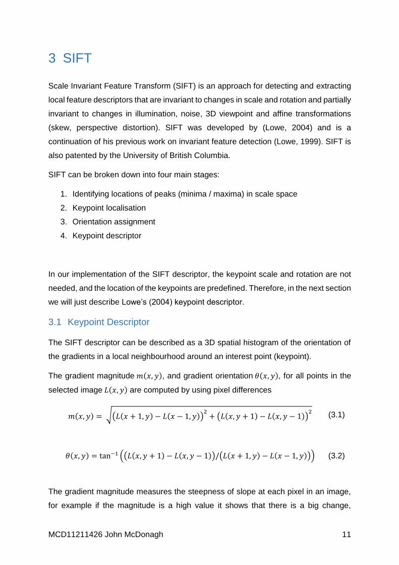
The SIFT descriptor can be described as a 3D spatial histogram of the orientation of
the gradients in a local neighbourhood around an interest point (keypoint).
The gradient magnitude 𝑚(𝑥, 𝑦), and gradient orientation 𝜃(𝑥, 𝑦), for all points in the
selected image 𝐿(𝑥, 𝑦) are computed by using pixel differences
𝑚(𝑥, 𝑦) = √(𝐿(𝑥 + 1, 𝑦) − 𝐿(𝑥 − 1, 𝑦))
2+ (𝐿(𝑥, 𝑦 + 1) − 𝐿(𝑥, 𝑦 − 1))
2 (3.1)
𝜃(𝑥, 𝑦) = tan−1 ((𝐿(𝑥, 𝑦 + 1) − 𝐿(𝑥, 𝑦 − 1))/(𝐿(𝑥 + 1, 𝑦) − 𝐿(𝑥 − 1, 𝑦))) (3.2)
The gradient magnitude measures the steepness of slope at each pixel in an image,
for example if the magnitude is a high value it shows that there is a big change,

MCD11211426 John McDonagh 12
whereas a low value means there is little to no change. The gradient orientation is the
angle made by the normal vector to the gradient surface in the direction of increasing
change and is measured in radians.
The gradient magnitudes, Equation (3.1) and orientations, Equation (3.2) are sampled
in a neighbourhood around the keypoint location on the selected image. Each sample
that is added to the histogram is weighted by its gradient magnitude multiplied by a
circular Gaussian kernel with a standard deviation equal to half the width of the
descriptor window. Lowe (2004) states that the purpose of the Gaussian window is to
avoid sudden changes in the descriptor with small changes in the position of the
window, and to give less emphasis to gradients that are far from the centre of the
descriptor, as these are most affected by misregistration errors.
Figure 3.1: For each 4x4 sub-region, the gradient magnitudes are weighted with the Gaussian filter (blue circle), the result of which is then added to the corresponding bin of the sub-region histogram that matches the gradient orientation. (Source: Gil, 2013)
Lowe (2004) uses a 16x16 local neighbourhood centred on a keypoint that is split into
4x4 sub-regions of 16 pixels each, Figure 3.1. Each sub-region is characterised by its
gradient contributions to an 8 bin orientation histogram, where each bin covers a 45-
degree range, giving a total of 360 degrees. The histogram can be sensitive to noise
if the orientation values are close to the boundaries of a bin, therefore to solve this
Lowe (2004) uses trilinear interpolation to distribute the value over two adjacent bins.
Finally, the 16 orientation histograms are concatenated to produce the 128 element
descriptor vector (16 sub-regions x 8 orientation bins).
To make the descriptor invariant to affine changes in illumination the vector is
normalised to unit length. Lowe (2004) also thresholds the values of the normalised

MCD11211426 John McDonagh 13
vector so that no value is above 0.2 and then re-normalises the vector. This is done to
reduce the influence of large gradient magnitudes and therefore put more emphasis
onto the distribution of gradient orientations.

MCD11211426 John McDonagh 14
4 Deformable Global Consensus Model
The propose system scans an image in a sliding window fashion and for each
candidate location it fits a generative facial deformable model using the current state-
of-the-art Project-Out Cascaded-Regression (PO-CR) algorithm which was proposed
by (Tzimiropoulos, 2015). Image locations that converge to the same location cast
votes for that location in a fashion similar to that of Hough Transform. After
thresholding the surface of votes, and performing non-maximal suppression (NMS) to
remove all the low scoring detections that refer to the same face, we end up with only
a few candidate locations per image. Next we calculate the median shape of the
candidate locations to produce a single fitted shape. Finally, the support vector
machine (SVM) scores are calculated by extracting both the Scale-Invariant Feature
Transform (SIFT) and colour features from around the landmarks of each of the fitted
shapes.
The main components of the proposed Deformable Global Consensus Model (DGCM)
are analysed as follows.
4.1 Shape model and appearance
DGCM uses Cascaded Regression (CR) to fit a deformable template to each sub-
window of a given image. The CR method that is used for this purpose is the recently
proposed PO-CR which has been shown to produce excellent fitting results for faces
with very large pose and expression variation. PO-CR uses parametric shape and
appearance models both learned with Principal component analysis (PCA).
4.1.1 Shape model
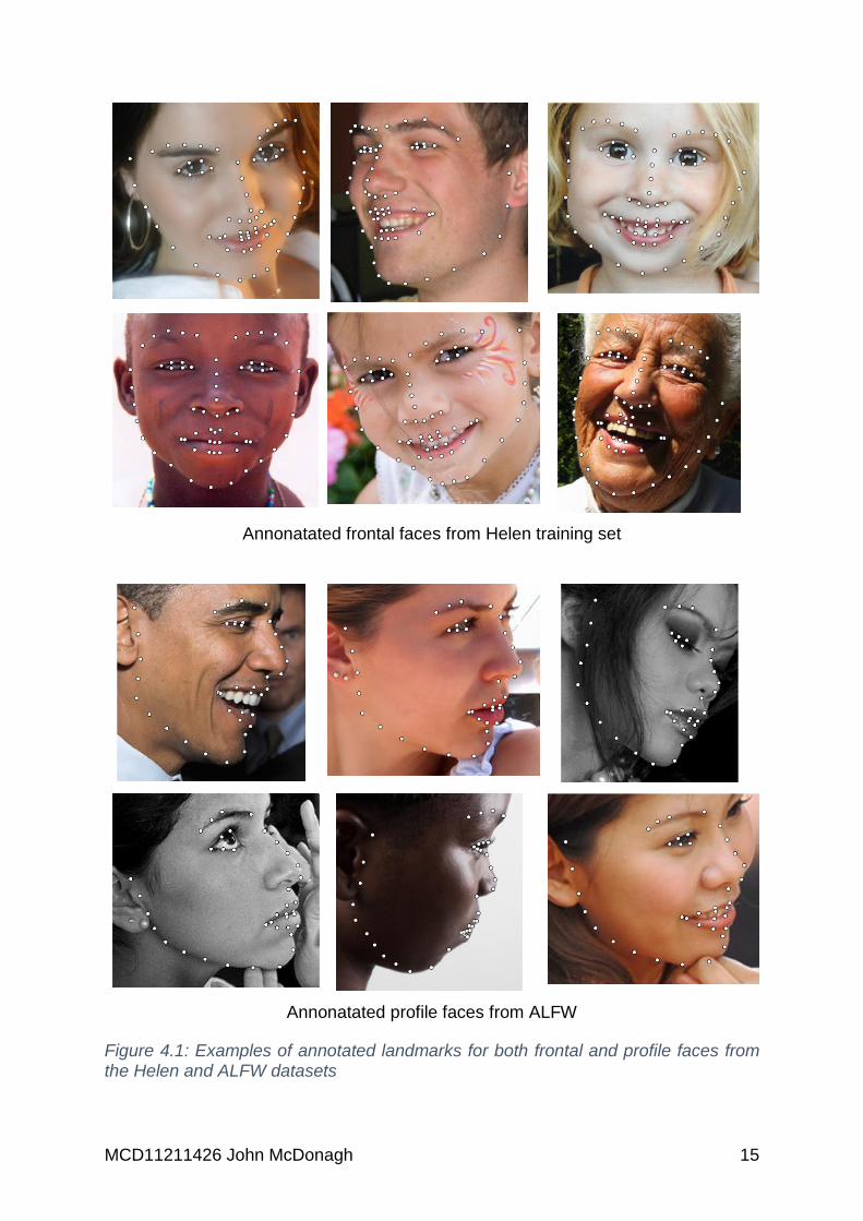
The shape model is first obtained by annotating a set of landmarks that are placed at
pre-defined locations which best describe the face. This is repeated over a set of
training facial images. Figure 4.1 shows examples of frontal and profile annotated
landmarks on various human faces.
MCD11211426 John McDonagh 15
Annonatated frontal faces from Helen training set
Annonatated profile faces from ALFW
Figure 4.1: Examples of annotated landmarks for both frontal and profile faces from the Helen and ALFW datasets
MCD11211426 John McDonagh 16
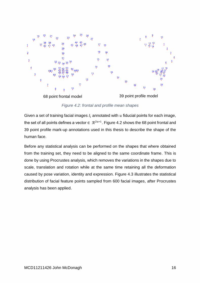
68 point frontal model
39 point profile model
Figure 4.2: frontal and profile mean shapes
Given a set of training facial images 𝐼𝑖 annotated with 𝑢 fiducial points for each image,
the set of all points defines a vector ∈ ℛ2𝑢∗1. Figure 4.2 shows the 68 point frontal and
39 point profile mark-up annotations used in this thesis to describe the shape of the
human face.
Before any statistical analysis can be performed on the shapes that where obtained
from the training set, they need to be aligned to the same coordinate frame. This is
done by using Procrustes analysis, which removes the variations in the shapes due to
scale, translation and rotation while at the same time retaining all the deformation
caused by pose variation, identity and expression. Figure 4.3 illustrates the statistical
distribution of facial feature points sampled from 600 facial images, after Procrustes
analysis has been applied.

MCD11211426 John McDonagh 17
Figure 4.3: Statistical distribution of facial feature points. The black dots represent 600 facial shapes that have been normalised by Procrustes analysis. The red dots signify the mean shape. (Wang et.al, 2014)
Once the shapes in the training set have been normalised, a statistical procedure
called Principal Component Analysis (PCA) is applied to obtain the shape model which
is defined by a mean shape 𝑠0 and a set of 𝑛 shape eigenvectors 𝑠𝑖 that are
represented as columns in 𝑆 ∈ ℛ2𝑢∗𝑛. These shape eigenvectors capture the
variations due to identity, pose and expression.
Finally, in accordance with (Mathews and Barker, 2004) a 2D similarity transform is
appended to the shape model, which has four similarity eigenvectors for scale, rotation
and translation.
Using this model, a shape can be instantiated by:
𝑠(𝑝) = 𝑠0 + 𝑆𝑝 (4.1)
Where 𝑝 ∈ ℛ𝑛∗1 is the vector of the shape parameters.
4.1.2 Appearance
To learn the appearance model that is used in PO-CR, similarity transformations are
removed from each facial training image 𝐼𝑖 this is achieved by warping the image to a
reference frame that is defined by the mean shape 𝑠0. As illustrated in Figure 4.4

MCD11211426 John McDonagh 18
Figure 4.4: Example of a face warped to the mean shape. The left image is the source image taken from a training set with the landmarks triangulated using Delaunay triangulation, the pixels within each triangle are then warped to the corresponding triangle in the mean shape. This gives us the shape-free texture, which is shown in the right image
Next, the local appearance around each landmark is encoded using SIFT (Lowe,
2004) and all the obtained descriptors are stacked in a vector ∈ ℛ𝑁∗1 which defines
the part-based facial appearance.
Finally, PCA is applied on all training facial images to obtain the appearance model
that is defined by the mean appearance 𝐴0 and 𝑚 appearance eigenvectors 𝐴𝑖 that
are represented as columns in 𝐴 ∈ ℛ𝑁∗𝑚. Using this model, a part-based facial
representation can be instantiated by:
𝐴(𝑐) = 𝐴0 + 𝐴𝑐 (4.2)
Where 𝑐 ∈ ℛ𝑚∗1 is the vector of the appearance parameters.
4.2 Deformable model fitting with PO-CR
We assume that a sub-window of our original image contains a facial image. We also
denote by 𝐼(𝑠(𝑝)) ∈ ℛ𝑁∗1 the vector obtained by generating 𝑢 landmarks from a shape
instance 𝑠(𝑝) and concatenating the computed SIFT descriptors for all landmarks.
To localise the landmarks in the given sub window, the shape and appearance models
are fitted by solving the following optimisation problem:
arg min𝑝,𝑐
‖𝐼(𝑠(𝑝)) − 𝐴(𝑐)‖2 (4.3)

MCD11211426 John McDonagh 19
As Equation (4.3) is non-convex, a locally optimal solution can be readily provided in
an iterative fashion using the Lucas Kanade algorithm that was originally proposed by
Matthews and Baker, (2004). In particular, given an estimate of 𝑝 and 𝑐 at iteration 𝑘,
linearization of Equation (4.3) is performed and updates, ∆𝑝, ∆𝑐 can be obtained in
closed form. Notably, one can by-pass the calculation of ∆𝑐 by solving
arg min∆𝑝
‖𝐼(𝑠(𝑝)) + 𝐽𝐼∆𝑝 − 𝐴0‖𝑃2 (4.4)
where ‖𝑥‖𝑃2 = 𝑥𝑇𝑃𝑥 is the weighted ℓ2-norm of a vector 𝑥. The solution to the above
problem is readily given by
∆𝑝 = −𝐻𝑃−1𝐽𝑃
𝑇(𝐼(𝑠(𝑝)) − 𝐴0) (4.5)
where the projected-out Jacobian matrix is 𝐽𝑃 = 𝑃𝐽𝐼 and the projected-out Hessian
matrix is 𝐻𝑃 = 𝐽𝑃𝑇𝐽𝑃 and 𝑃 = 𝐸 − 𝐴𝐴𝑇 is a projection operator that projects out the facial
appearance variation from the image specific Jacobian 𝐽𝐼, and 𝐸 is the identity matrix.
Given that 𝑛 is the number of shape parameters, 𝑚 is the number of appearance
parameters and 𝑁 is the number of SIFT features, the above algorithm has a
complexity 𝑂(𝑛𝑚𝑁 + 𝑛2𝑁) per iteration and can be implemented in real-time for a
single fitting. But, it is too slow to be employed for all sub-windows of a given image.
The reason for this is because the Jacobian matrix, and the inverse Hessian matrix
needs to be computed for each iteration.
PO-CR bypasses this computational burden by pre-computing the averaged
projected-out Jacobian and Hessian matrices for each iteration using regression.
In particular, for each iteration 𝑘 PO-CR pre-computes the averaged projected-out
Jacobian matrix, denoted as 𝐽𝑝(𝑘) as described by (Tzimiropoulos, 2015) which in
turn, is then used to pre-calculate the averaged projected-out Hessian matrix, denoted
as ��𝑝(𝑘), as follows
��𝑝(𝑘) = 𝐽𝑝(𝑘)𝑇𝐽𝑝(𝑘) (4.6)

MCD11211426 John McDonagh 20
Finally, the descent directions, denoted as 𝑅(𝑘) for each iteration can then be pre-
computed by using the inversed average Hessian matrix and average Jacobian matrix
𝑅(𝑘) = ��𝑝(𝑘)−1𝐽𝑝(𝑘)𝑇 (4.7)
During testing, given a current estimate of the shape parameters at iteration 𝑘, denoted
as 𝑝(𝑘), the image features 𝐼(𝑠(𝑝(𝑘)))) are extracted and then an update for the shape
parameters, ∆𝑝(𝑘) can be computed as follows
∆𝑝(𝑘) = 𝑅(𝑘)(𝐼(𝑠(𝑝(𝑘))) − 𝐴0) (4.8)
Since the descent directions 𝑅(𝑘) are pre-computed and 𝐴0 is a constant template
representing the mean facial appearance, it is possible to precompute the bias term,
denoted as 𝐶(𝑘) for each iteration
∆𝑝(𝑘) = 𝑅(𝑘)𝐼(𝑠(𝑝(𝑘))) − 𝑅(𝑘)𝐴0 (4.9)
𝐶(𝑘) = 𝑅(𝑘)𝐴0 (4.10)
which in turn gives the equation
∆𝑝(𝑘) = 𝑅(𝑘)𝐼 (𝑠(𝑝(𝑘))) − 𝐶(𝑘) (4.11)
where 𝑠(𝑝(𝑘)) is the shape at iteration 𝑘, and 𝑅(𝑘) ∈ ℛ𝑛∗𝑁 and 𝐶(𝑘) ∈ ℛ𝑛∗1 are the
descent directions and the bias term for iteration 𝑘 learned from data using regression.
Next, a new estimate for the shape parameters that are used in the next iteration are
obtained from
𝑝(𝑘 + 1) = 𝑝(𝑘) − ∆𝑝(𝑘) (4.12)
Finally, after 𝐿 iterations the fitted shape is obtained. Using the above projected-out
cascade regression method, the fitting can be achieved with a computational cost of
only 𝑂(𝑛𝑁). Figure 4.5 demonstrates the high level overview of the proposed
Deformable Global Consensus Model.

MCD11211426 John McDonagh 21
Figure 4.5: Overview of the proposed Deformable Global Consensus Model. For each iteration, if the current threshold is above zero, Hough-Transform voting is used to reject any shapes peaks below the threshold.

MCD11211426 John McDonagh 22
4.3 Training
For learning 𝑅(𝑘), the training sets of Helen and LFPW plus the available landmark
annotations of the 300-W challenge where used to generate the frontal model. This
made it possible to fit faces with very large yaw variation (±70°). Because the frontal
model could not achieve ±90° yaw, another profile model was generated from 1,000
manually annotated profile images from the ALFW dataset.
4.4 Hough-Transform Voting
The proposed DGCM detects faces via a Hough Transform voting scheme by
capitalising on the properties of the iterative optimisation procedure employed by PO-
CR. The system scans an image in a sliding window fashion using a step of 10 pixels
in both the (x, y) dimensions. At each location that is sampled using the sliding window,
a facial deformable model is fitted using PO-CR.
Because of the large basin of attraction of regression based approaches, shapes that
are initialised close to a face will very likely converge with a high degree of accuracy
to that face. On the contrary, shapes that are initialised to the background will converge
to random locations. Hence this process will generate a high number of votes for any
face within an image, while at the same time will score a low number of votes for
background.
Voting in the proposed system is performed in a straight forward fashion. At each
iteration the location of the shapes in the image are found by extracting the
translational component from 𝑝 and then for each location a vote is cast. Next, for each
iteration, any shapes that belong to a peak that does not pass the threshold value for
that iteration are rejected. Finally, because we end up with multiple detections per
peak, we apply non-maximum suppression (NMS) (Felzenszwalb, et al., 2010) to
reject all low scoring detections that refer to the same face. After which we are left with
just a few candidate face locations per image.
For non-maximum suppression (NMS) we adopt a strategy similar to Felzenszwalb, et
al., (2010) where we sort scores in descending order, and then iteratively select the
detection window with the highest score, while eliminating detected windows with an

MCD11211426 John McDonagh 23
intersection-over-union (IoU) ratio greater than a predefined threshold to the currently
selected detection window.
4.5 Final re-scoring
After the voting phase is finished, we are left with only a few candidate locations. For
each of these locations, the median shape is calculated form all the corresponding
shapes of each peak, to produce a single fitted shape for that location. Finally, once
the final fitted shapes have been obtained, re-scoring of the candidate faces is
performed by evaluating an SVM that is trained on both the SIFT features, and the U
channel of the LUV colour space as proposed by (Mathias, et al., 2014).
4.6 Complexity
We assume that there are 𝑘 levels of cascade in the PO-CR model. Then, for each
level, a regression matrix 𝑅(𝑘) is learned with 𝑛 regressors and 𝑁 SIFT features. As
stated previously, 𝑛 is the number of parameters in the shape model. Therefore, the
complexity of fitting per sub-window is only 𝑂(𝐾(𝑛𝑁)).
Because of the large basin of attraction of PO-CR, fitting is performed on a grid of
equally spaced points, with a stride of 10 pixels in both the (x, y) dimensions. If there
are 𝐿 locations per image to perform fitting, then the total complexity becomes
𝑂(𝐿𝐾(𝑛𝑁)) for a single level of the image pyramid.
Furthermore, since the first level of the cascade is optimised for only scale, rotation
and translation, and applying a threshold after casting votes in Hough space. The
proposed method can reject most of the irrelevant background in the image, which in
turn leaves very few locations to be evaluated in the subsequent levels of the cascade.
Hence, in practice, the total complexity is 𝑂(𝐿𝐾(𝑛𝑁)) where 𝐾 = 1 and 𝑛 = 4

MCD11211426 John McDonagh 24
5 CUDA
In order for the reader to get a good understanding of the fundamentals of parallel
programming on the GPU, which is used in this thesis, this chapter introduces the
reader to the hardware and software architecture of the CUDA API. We also invite the
reader to read Appendix A which gives an in-depth comparison between CUDA and
OpenCL, and the reasons why CUDA was chosen over OpenCL.
CUDA stands for Compute Unified Device Architecture and is a parallel programming
paradigm, the initial CUDA toolkit 1.0 was release in June 2007 (NVIDIA, 2016).
CUDA is used to develop software that utilises the power of NVIDIA GPU’s and cannot
be used on GPU’s made by any other vendor. As well as graphics, CUDA is also used
in many general-purpose, non-graphical applications that are highly parallel in nature.
CUDA uses C/C++ as its main programming language, although it also can be
programed on other languages like FORTRAN and Java. Since the initial release in
2007, there have been 7 major releases of the CUDA toolkit along with four major
hardware revisions; Tesla, Fermi, Kepler and Maxwell.
5.1 CUDA architecture
Figure 5.1: Kepler GK110 Full chip block diagram (Source: NVIDIA, 2012, p6)

MCD11211426 John McDonagh 25
The architecture of the GeForce 780ti as illustrated in Figure 5.1 consists of 5 Graphics
Processing Clusters (GPC), each containing 3 streaming multiprocessors (SMX),
which gives a total of 15 SMX units. Shared 1.5MB L2 cache which can be accessed
by all SMX units, six 64-bit memory controllers which gives a combined 384-bit
memory interface, that is connected to 3GB of GDDR5 device memory. A Host
interface which connects the GPU to the CPU via a PCI-express v3.0 bus and
NVIDIA’s trademarked GigaThread Engine, which creates and dispatches thread
blocks to the various SMX units and manages the context switches between threads
during execution.
5.1.1 Streaming multiprocessor (SMX)
Figure 5.2: SMX: 192 single‐precision CUDA cores, 64 double‐precision units, 32 special function units (SFU), and 32 load/store units (Source: NVIDIA, 2012, p8)
As shown in Figure 5.2, the SMX unit on the GK110 GPU contains a total of 192 single-
precision CUDA cores and 64 double-precision units (DP Unit) which perform
arithmetic operations in accordance to the IEEE 754-2008 standard. There are also
32 load/store units (LD/ST) which are used to move data between registers, shared
memory and global memory, and 16 special function units (SFU’s) which are used for

MCD11211426 John McDonagh 26
fast approximations of transcendental operations, such as, sin, cosine, reciprocal and
square root.
Each SMX also includes 65,536 32-bit registers, an instruction cache, 64 KB of high
speed memory that can be partitioned between the L1 cache and shared memory by
the developer, and 48 KB of high speed read only data cache memory that is shared
by all the CUDA cores on the SMX unit. There are also four warp schedulers and eight
instruction dispatch units. The warp schedulers make it possible to issue and execute
four concurrent warps, and the instruction dispatch units make it possible to execute
two independent instructions of a warp per cycle.
5.2 Compute Capability
NVIDIA use a special term called compute capability to describe different hardware
versions of their GPU’s. As show in Table 5.1 CUDA comes in several different
versions each mapping to a different generation of GPU. Older GPU architectures will
not work with a program compiled for higher compute capability devices, however
CUDA is backward compatible. With each new revision comes new features and
technical specifications.
Architecture Codename Compute Capability Released
Tesla G80
GT200
1.0
1.3
2006
2008
Fermi GF100
GF104
2.0
2.1
2010
2010
Kepler GK104
GK110
3.0
3.5
2012
2013
Maxwell GM107
GM204
GM200
5.0
5.2
5.2
2014
2014
2015
Table 5.1: CUDA Compute Capability
5.3 Kernel Functions
CUDA extends C by allowing the programmer to define C functions which are called
kernels, these kernels can only be executed on the GPU, but unlike standard C

MCD11211426 John McDonagh 27
functions they cannot have a return type. The kernel is defined using the __global__
declaration specifier and the number of threads that execute within the kernel for a
given call is specified using the <<<…..>>> execution configuration syntax.
When a kernel function is launched, it creates an array of multiple threads, these
threads are mapped to the processor and executed in what NVIDIA call Single-
Instruction, Multiple-Thread (SIMT). This is similar to Single-Instruction, Multiple-
Data (SIMD), but whereas SIMD requires that all elements in a vector execute
together in a unified synchronous group, SIMT allows multiple threads in the same
warp to execute independently.
5.4 Thread hierarchy
When a kernel is launched, it is organised into a two-level hierarchy of threads, where
the threads are grouped into blocks called thread blocks, and the thread blocks are
grouped into a grid, as illustrated in Figure 5.3. There can only be one grid per Kernel.
The dimensions of the grid, and thread blocks within the grid, are specified via the
execution configuration parameters at kernel launch time by the developer and cannot
change throughout the life time of the kernel.
MCD11211426 John McDonagh 28
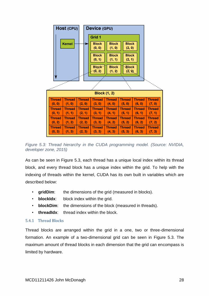
Figure 5.3: Thread hierarchy in the CUDA programming model. (Source: NVIDIA, developer zone, 2015)
As can be seen in Figure 5.3, each thread has a unique local index within its thread
block, and every thread block has a unique index within the grid. To help with the
indexing of threads within the kernel, CUDA has its own built in variables which are
described below:
• gridDim: the dimensions of the grid (measured in blocks).
• blockIdx: block index within the grid.
• blockDim: the dimensions of the block (measured in threads).
• threadIdx: thread index within the block.
5.4.1 Thread Blocks
Thread blocks are arranged within the grid in a one, two or three-dimensional
formation. An example of a two-dimensional grid can be seen in Figure 5.3. The
maximum amount of thread blocks in each dimension that the grid can encompass is
limited by hardware.

MCD11211426 John McDonagh 29
Thread blocks are required to execute independently from one another, this is because
they are distributed randomly to the various SMX units, as and when resources
become available. A maximum of sixteen thread blocks can run concurrently in a SMX,
but there are several factors that limit this amount, such as the amount of threads,
registers and shared memory used per block. Also, it must be noted that because
multiple thread blocks execute in parallel, care must be taken to avoid race conditions
when writing to global memory, this can be achieved with the use of atomic operators.
5.4.2 Threads
Thread blocks are made up of a collection of threads which run on the CUDA cores.
Current hardware supports a maximum of 1024 threads per block which can be
arranged in a one, two or three-dimensional formation.
Within a thread block, threads are divided into groups of 32 consecutive threads called
warps. The order the warps execute in within the block is random. Threads are only
allowed to communicate with other threads in the same block by the use of shared
memory. Threads within a warp can also communicate directly with each other using
warp level intrinsics. For compute capability 3.0 and above, each thread can have
access to a maximum of 255 32-bit registers that are only visible to the thread that
they reside in.
The total number of threads that a given kernel executes is equal to the number of
threads per block multiplied by the total number of thread blocks. For example, if the
execution configuration parameters are set to <<<1024, 256>>> then there will be
1024 thread blocks multiplied by 256 threads, which gives a total of 262,144 threads,
executing the same kernel.
5.5 Memory Hierarchy
In the CUDA programming model for the Kepler architecture, the memory hierarchy is
composed of four distinct levels, which is illustrated in Figure 5.4. These four levels
are from top to bottom (fastest to slowest): the thread level, SMX level, a global level
2 cache and lastly the large global DRAM memory of the GPU.
MCD11211426 John McDonagh 30
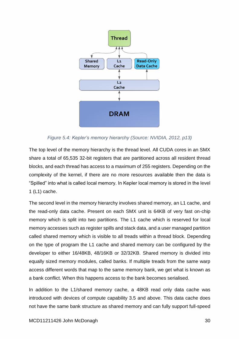
Figure 5.4: Kepler’s memory hierarchy (Source: NVIDIA, 2012, p13)
The top level of the memory hierarchy is the thread level. All CUDA cores in an SMX
share a total of 65,535 32-bit registers that are partitioned across all resident thread
blocks, and each thread has access to a maximum of 255 registers. Depending on the
complexity of the kernel, if there are no more resources available then the data is
“Spilled” into what is called local memory. In Kepler local memory is stored in the level
1 (L1) cache.
The second level in the memory hierarchy involves shared memory, an L1 cache, and
the read-only data cache. Present on each SMX unit is 64KB of very fast on-chip
memory which is split into two partitions. The L1 cache which is reserved for local
memory accesses such as register spills and stack data, and a user managed partition
called shared memory which is visible to all treads within a thread block. Depending
on the type of program the L1 cache and shared memory can be configured by the
developer to either 16/48KB, 48/16KB or 32/32KB. Shared memory is divided into
equally sized memory modules, called banks. If multiple treads from the same warp
access different words that map to the same memory bank, we get what is known as
a bank conflict. When this happens access to the bank becomes serialised.
In addition to the L1/shared memory cache, a 48KB read only data cache was
introduced with devices of compute capability 3.5 and above. This data cache does
not have the same bank structure as shared memory and can fully support full-speed

MCD11211426 John McDonagh 31
unaligned memory access patterns. Use of this cache can be managed automatically
by the compiler if it can determine if the data is read only for the life time of the kernel,
this is done by qualifying pointers as const and __restrict__, or explicitly by the
programmer by using the __ldg() intrinsic function.
The third level in the memory hierarchy contains the global level 2 (L2) cache which
has a size of 1.5MB. This cache is the primary point of data unification between all
SMX units on the GPU, servicing all load, store, and texture requests to DRAM and
providing efficient, high speed data sharing across the GPU. The caching policy which
is used is called least recently used (LRU), the main intention of which is to avoid the
global memory bandwidth bottleneck (Farber, 2012, p.113).
The bottom level in the memory hierarchy is the DRAM. This is the physical device
memory (3GB GDDR5 on the GeForce 780ti) built on the graphics card. Device
memory is off-chip and is significantly slower compared to the higher levels in the
hierarchy. All threads have access to device memory.
There are also two read-only memory spaces in DRAM which are called constant and
texture memory, which can also be accessed by all threads of the GPU. Both constant
and texture memory are cached and optimised for different usages. Constant memory
is optimised for broadcasting, i.e. when the threads in a warp all read the same
memory location, whereas texture memory is optimised for spatial locality.
Constant memory resides in a 64 KB partition of device memory and is accessed
through an 8KB cache on each SMX. The texture cache is limited to 48 KB per SMX
unit. Both constant and texture memory are persistent across all kernel launches by
the same application.

MCD11211426 John McDonagh 32
6 Implementation
The proposed system is executed within the MATLAB environment, and Mex-files are
used to provide an interface to the CUDA C++ algorithms. Figure 6.1 shows a high
level view of the proposed system.
Figure 6.1: System overview, the red outlined boxes are the Mex functions that are used to provide an interface to CUDA C++
MCD11211426 John McDonagh 33
Given an RGB image, we first use MATLAB to generate a grey scale image. The RGB
image is also converted to LUV colour space using the Mex function “colorspace” that
was created by Getreuer, (2010), and then the U channel is extracted to be later used
in extracting features for the SVM model.
The proposed system needs to iterate three times to cover both frontal and profile
(right and left) faces. The three iterations are as follows:
1. Frontal
2. Right profile
3. Left profile
As there are only two models used in the system, a frontal and a right facing profile
model, to cover left facing profile faces, the input images (grey scale, U channel) are
flipped on the third iteration.
The current model and grey scale image are next passed into the DGCM Mex function,
which provides an interface to the CUDA C++ code. DGCM scans the grey scale
image over multiple scales, in a sliding window fashion using a step of 10 pixels in
both the (x, y) dimensions. For each scale, all sub-windows are simultaneously fitted
using the PO-CR algorithm.
After each iteration of the PO-CR algorithm, votes are cast using a Hough-Transform
voting scheme for detecting candidate faces and filtering out irrelevant background.
For each scale, NMS is applied to remove low level peaks that are within the vicinity
of the maxima peaks. Next, the median of the shapes corresponding to each surviving
peak is calculated to produce a single fitted shape for each maxima peak. Then the
surviving candidate shapes are sent back to MATLAB for further processing.
The remaining candidate shapes are then rescaled back into image space and the left
facing profile shapes are flipped back to their original direction. Next, NMS is applied
to the remaining candidate shapes to remove low SVM scoring shapes of faces from
the wrong scales and then a final NMS is applied on the combined front, left and right
shapes. Finally, the performance of the system is evaluated.

MCD11211426 John McDonagh 34
6.1 DGCM
The proposed Deformable Global Consensus Model (DGCM) as described in Chapter
4 is implemented in CUDA using two distinct levels of parallelisation. The reason for
this is because all the windows of the grid are independent from one another, therefore
they can be processed simultaneously, and this is achieved by essentially dedicating
one thread block to each instance of the PO-CR fitting algorithm.
6.1.1 Memory allocation
All matrices that are used in the DGCM model are allocated in device memory using
the CUDA function call “cudaMallocPitch”. This guarantees that all the rows of the
matrices meet the alignment requirements for coalesced memory accesses. This is
achieved by allocating bytes at the end of each row to guarantee that the beginning of
the next row starts on a 128 byte memory boundary, as illustrated in Figure 6.2. The
pitch is the width of the row including padding measured in bytes.
Figure 6.2: 2D matrix allocation. When allocating device memory via the cudaMallocPitch function call, rows are padded (yellow blocks) to guarantee that the beginning of each row begins on a 128 memory boundary.
6.1.2 SIFT
The SIFT descriptor used in this implementation is a variant of Lowes (2004) SIFT
keypoint descriptor which is described in Chapter 3.1. Where the main difference is,
instead of having a grid containing 16 blocks, that output a 128 element descriptor as
shown in Figure 3.1, our variant of Lowes, (2004) descriptor only uses one 8x8
dimensional block, which outputs an 8 element descriptor.

MCD11211426 John McDonagh 35
We pre-calculate SIFT descriptors for each pixel in the image and store the results in
a texture, which is then used as a look up table. We use texture memory because it is
optimised for 2D spatial locality. The pre-calculated SIFT descriptors are stored in a
2D layered texture which has a depth of two. As there are eight descriptor elements
per pixel, each layer contains a RGBA texture to hold four descriptors elements.
6.1.3 PO-CR
Given Equation 4.11 and Equation 4.12, the CUDA implementation of the PO-CR
fitting algorithm can be broken down into just five stages that consist of four bespoke
kernels, which are, for each iteration 𝑘:
Stage 1
Calculate the current estimate of the shape parameters 𝑝(𝑘). Were 𝑠(𝑝(𝑘 − 1)) is the
shape generated from the previous iteration, 𝑆0 is the mean shape and 𝑄(𝑘) ∈ ℛ2𝑢∗𝑛
contains the combination of the similarity eigenvectors for scale, rotation and
translation and the shape eigenvectors
𝑝(𝑘) = 𝑄(𝑘)𝑇 ∗ (𝑠(𝑝(𝑘 − 1)) − 𝑆0) (6.1)
Stage 2
Calculate the current shape 𝑠(𝑝(𝑘)), from the estimate of the shape parameters 𝑝(𝑘)
that are obtained from Equation (6.1)
𝑠(𝑝(𝑘)) = 𝑆0 + (𝑄(𝑘) ∗ 𝑝(𝑘)) (6.2)
Stage 3
Extract the SIFT features 𝐼 (𝑠(𝑝(𝑘))) ∈ ℛ𝑁∗1 for the current shape, where 𝑁 is the
number of features.
𝐼 (𝑠(𝑝(𝑘))) (6.3)
Stage 4

MCD11211426 John McDonagh 36
Update the estimate of the shape parameters. Where 𝑅(𝑘) and 𝐶(𝑘) are the descent
directions and bias term as described in Chapter 4.2
𝑝(𝑘) = 𝑝(𝑘) − ((𝑅(𝑘) ∗ 𝐼 (𝑠(𝑝(𝑘)))) − 𝐶(𝑘)) (6.4)
Stage 5
Equation (6.2) is again used to calculate the new shape, using the updated shape
parameters 𝑝(𝑘) obtained from Equation (6.4)
With the exception of stage 3, in each stage of the PO-CR fitting algorithm the kernel
is launched with just one thread block to do all the work in parallel.
The dimensions of the thread block in Equation (6.1) and Equation (6.4) is (32, 𝑛, 1)
where 32 is the size of a warp and 𝑛 is the current number of shape parameters 𝑝(𝑘).
Each row in the thread block calculates the scalar output of the corresponding
component of 𝑝
In Equation (6.2) the thread block size depends on the amount of points in the shape
model, for the 68 point frontal model it is set to (136,1,1) and for the 39 point profile
model it is set to (78,1,1).
In Equation (6.3) the thread block size is (256,1,1) and the total number of thread
blocks used is calculated by the formula 1 + (((𝑁 / 4) − 1) / 256) we divide the
number of features 𝑁 by four because we use vectorise access to read four SIFT
descriptor elements at a time from texture memory. The value 256 is taken from the
thread block’s x-dimension.
6.1.4 CUDA Vector-Matrix multiplication
In order to solve Equation (6.1), Equation (6.2) and Equation (6.4), we use vector-
matrix multiplication. Given a matrix 𝑀 and a vector 𝑣, it is possible to work out each
component of 𝑦 by calculating the dot product of row 𝑖 of matrix 𝑀 with 𝑣.
𝑦𝑖 = ∑ 𝑀𝑖,𝑗
𝑛
𝑗=1
𝑣𝑗 (6.5)

MCD11211426 John McDonagh 37
In parallel computing a dot product can be solved with the use of the reduction
primitive. Reduction is one of the most used primitives in parallel computing, it is used
to reduce a data sequence into a scaler value using a binary associative operator. It
can be used for example to compute the minimum, maximum and sum of two vectors.
Because reduction involves very little processing, it is beneficial to have each thread
process multiple elements before doing the actual reduction. This is achieved by each
thread reading elements in the arrays in a grid-stride loop (Harris, 2013), and can be
further optimised by using vectorised accesses to global memory. Once the loop is
completed, then the reduction can be done and the scaler result can be output back
to global memory. The code used in this thesis for calculating the dot products is based
on a warp shuffle reduction that was explained by Luitjens (2014). Figure 6.3 shows
an example of warp shuffle reduction.
Figure 6.3: Warp reduction using shuffle down, for illustrative purposes this figure only shows a half warp (16 lanes). The first parameter of the __shfl_down intrinsic is the register to return, the second is the offset from the calling lane of the warp and the third parameter is the width of the warp segment which must be of size 2, 4, 8, 16, or 32. The default size is 32.

MCD11211426 John McDonagh 38
Figure 6.3 shows how the shuffle down intrinsic is used to build a reduction tree inside
a warp. The shuffle down intrinsic first calculates the source lane’s ID by adding an
offset to the calling lane’s ID, and then returns the value held at that location. If the
source lane is out of bounds or the source thread has finished, then the value in the
calling thread is returned instead. The value that is returned from the source lane is
then added to the calling lanes register. Finally, after completing the reduction tree,
the thread in lane zero contains the sum of the warp.
6.1.5 Voting
After each iteration of the PO-CR algorithm, the Hough-Transform voting surface is
cleared. Next, the location of the shapes in the image are found by extracting the
translational component from 𝑝 and then for each location a vote is cast within an
11*11 grid. Thus, generating peaks on the voting surface, as illustrated in Figure 6.5.
Next, any shapes that belong to peaks that do not pass the threshold for the current
iteration are rejected, as shown in Figure 6.6 to Figure 6.9. By doing this, it is possible
to remove most of the background windows within the first few iterations where the
computational cost of calculating ∆𝑝(𝑘) is relatively cheap. Figure 6.10 shows the SVM
scores generated for each peak and Figure 6.11 shows the final fitted shape after a
threshold has been applied.
Figure 6.4: Original image from the AFW dataset
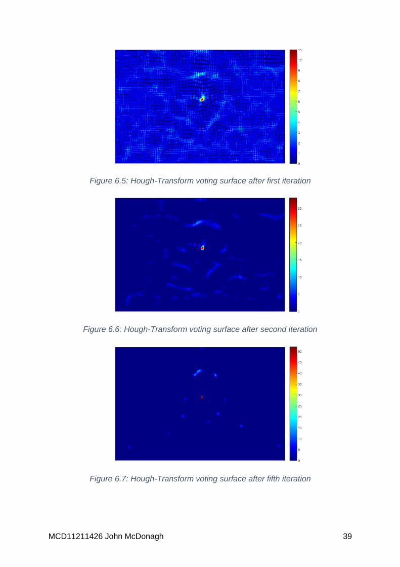
MCD11211426 John McDonagh 39
Figure 6.5: Hough-Transform voting surface after first iteration
Figure 6.6: Hough-Transform voting surface after second iteration
Figure 6.7: Hough-Transform voting surface after fifth iteration

MCD11211426 John McDonagh 40
Figure 6.8: Hough-Transform voting surface after tenth iteration
Figure 6.9: Hough-Transform voting surface after fifteenth iteration
Figure 6.10: SVM scores generated for candidate faces

MCD11211426 John McDonagh 41
Figure 6.11: Final fitted results after threshold has been applied
In order to remove shapes that have failed the threshold for the current iteration, each
shape acquires its vote’s score from the Hough-Transform voting surface and stores
the result in a votes array. Next, an index array is generated by scanning the votes
array and storing the indices of votes that pass the threshold, the indices of votes that
fail the threshold are set to minus one, as shown in Figure 6.12.
Figure 6.12: Stream compaction. Any vote score (yellow boxes) with a value equal or less than one is set to minus one in the index array, then the function copy_if from the thrust library is used to compact the array.
To compact the index array the function “copy_if” from the Thrust library is used, with
the predicate parameter set to minus one. The output of which is a compacted index

MCD11211426 John McDonagh 42
array. Finally, the new compacted index array is used to get the shapes that pass the
threshold.
6.2 Support Vector Machine (SVM)
LIBSVM was used for support vector classification. LIBSVM is an open source library
developed at the National Taiwan University. Since version 2.8, it implements a
sequential minimal optimisation (SMO) type algorithm which was proposed by (Chang
and Lin, 2011).
SVM belongs to the class of maximum margin classifiers and are capable of solving
linear and non-linear classification problems. SVMs map data to feature space with
the use of kernels. There are four basic kernel functions, linear, polynomial, radial
basis function (RBF) and sigmoid.
Given a training set of vectors 𝑥𝑖 ∈ ℛ𝑛, 𝑖 = 1, ⋯ , 𝑙 where each vector belongs to one
of two classes that are identified by the label 𝑦𝑖 ∈ {−1, 1}. The aim of SVM
classification is to separate both classes with an optimal separating hyperplane in such
a way that the distance to the support vectors is maximised, as illustrated in Figure
6.13, called the maximum margin.
Figure 6.13: Optimal separating hyperplane, the three filled in shapes are the support vectors (Source: OpenCV, 2016)

MCD11211426 John McDonagh 43
While optimising an SVM, we are generally looking for two things: a hyperplane with
the largest margin, and also a hyperplane that produces the minimum amount of
misclassification errors.
The penalty parameter 𝐶 is a regularisation parameter that controls the cost of
misclassification on the training data. Having a low 𝐶 value generates a large margin
separation hyperplane, at the cost of misclassification. While a high 𝐶 value gives a
smaller margin if it does a better job of classifying the training points correctly. Finding
the optimal 𝐶 value while minimising overfitting is generally done with the use of cross-
validation.
6.2.1 Feature normalisation
Before using cross validation to find the optimal value of 𝐶, both the SIFT and colour
features (LUV colour space, U channel) (Mathias et al, 2014) needs to be normalised.
We found that the best method to normalise these features was to use zero-mean ℓ2-
norm. This is achieved by first, calculating the zero-mean
𝜇 = 1
𝑁⁄ ∑ 𝑥𝑖
𝑁
𝑖=1
(6.6)
𝑥𝑖 = 𝑥𝑖 − 𝜇 (6.7)
Next, the features are normalised, and weight adjusted, for SIFT Vectors the value of
𝑤 is set to 1 and for the colour vectors 0.2 is used
𝑥𝑖 = (𝑥𝑖/|𝑥|) ∗ 𝑤 (6.8)
Finally, the normalised SIFT and colour features are combined into a single vector.
6.2.2 Cross-validation
LIBSVM has an option –v to set the number of folds to use in cross-validation. For
example, using –v 5 creates 5-folds, where the training data is split into 5 equally sized
subsets, and each subset is then tested using a classifier trained on the remaining 4
subsets.

MCD11211426 John McDonagh 44
In order to find the optimal 𝐶 value and prevent overfitting, a grid-search on 𝐶 is
performed using cross-validation. This is done by first scanning a coarse 1-
dimensional grid to find the highest cross validation accuracy region. Then, a finer
scan is conducted in that region to find the optimal 𝐶 value. Once the optimal 𝐶
parameter has been found the model can be trained using all the training data.
6.2.3 Training
For training the SVM model, a two-step approach was used. First, DGCM scans the
training sets and then all the fitted shapes are stored in the positive class. The negative
class is obtained by sorting the votes of the background shapes in descending order,
next they are truncated it to match the size of the positive class, then a SV is trained.
Next, DGCM is again used to scan the training sets, but this time it also calculates the
SVM scores for the shapes. As before, the shapes are split into positive and negative
classes, but this time the negative class is sorted in descending order using the SVM
scores. Finally, the negative class is truncated to match the size of the positive class,
before generating the final SVM model.
6.2.4 Classification
Once the optimal separating hyperplane has been found, the SVM can attempt to
classify unseen data. Given an instance 𝑧 it can be classified by determining which
side of the decision boundary it belongs to, by computing the following decision
function
𝑓(𝑧) = 𝑠𝑖𝑔𝑛 ( ∑ 𝑦𝑖𝛼𝑖𝑘(𝑥𝑖, 𝑧)
𝑡𝑜𝑡𝑎𝑙𝑆𝑉
𝑖=1
+ 𝜌) = 𝑠𝑖𝑔𝑛(𝑤𝑇𝜙(𝑧) + 𝜌) (6.9)
where 𝑦 is the training labels, 𝛼 contains the support values, 𝑘(. , . ) is the kernel
function, 𝜌 is the offset from the origin and 𝑤 defines the normal to the hyperplane.
Within the LIBSVM model that is generated in the training phase, 𝑠𝑣_𝑐𝑜𝑒𝑓
contains 𝛼𝑖𝑦𝑖, 𝑆𝑉𝑠 contains the support vectors 𝑥𝑖, and – 𝑟ℎ𝑜 is the 𝜌 value
Using a linear kernel 𝑘(𝑥, 𝑧) = 𝑥𝑇𝑧 it is possible to compute 𝑤 explicitly using
𝑤 = 𝑆𝑉𝑠𝑇 ∗ 𝑠𝑣_𝑐𝑜𝑒𝑓 (6.10)

MCD11211426 John McDonagh 45
Therefore, all predictions are simply based on the function.
𝑧𝑇𝑤 + 𝜌 (6.11)
If the score is larger than the defined threshold we then classify the candidate
window as a face.

MCD11211426 John McDonagh 46
7 Results
In order to evaluate the performance of our proposed system, all tests were done using
a NVIDIA GeForce GTX 980 GPU and an Intel I7-4790k CPU, on a PC running
Windows 8.1 64-bit with 16GB of ram. The proposed system was compiled for GPU
devices of compute capability 3.5 and above, using CUDA 7.0 development toolkit.
7.1 Performance measures
For face detection, faces are only considered detected if the intersection-over-union
(IoU) ratio between the ground truth and the detected bounding box/ellipse exceeds
0.5 (50%) (Everingham et al, 2009). Given a detected bounding box 𝐵𝑑 and ground
truth bounding box 𝐵𝑔𝑡 the area of overlap 𝑎𝑜 can be found using the formula
𝑎𝑜 =𝑎𝑟𝑒𝑎(𝐵𝑑 ∩ 𝐵𝑔𝑡)
𝑎𝑟𝑒𝑎(𝐵𝑑 ∪ 𝐵𝑔𝑡)
where the intersection 𝐵𝑑 ∩ 𝐵𝑔𝑡 is the area of overlap between the detected and
ground truth bounding boxes and the union 𝐵𝑑 ∪ 𝐵𝑔𝑡 is the sum of the areas of both
bounding boxes minus the intersection.
To evaluate the performance of our experiments for face detection on the AFW
dataset, we use a precision-recall (PR) curve to extract the relationship between the
detection rate (recall) and detection accuracy (precision).
Precision and Recall are defined as:
𝑝𝑟𝑒𝑐𝑖𝑠𝑖𝑜𝑛 =𝑇𝑃
𝑇𝑃 + 𝐹𝑃
𝑟𝑒𝑐𝑎𝑙𝑙 =𝑇𝑃
𝑇𝑃 + 𝐹𝑁
Where true positives 𝑇𝑃 are faces that are correctly classified. False positives 𝐹𝑃 is
where the detector wrongly classifies background as a face, and false negatives 𝐹𝑁
are faces that are not detected.
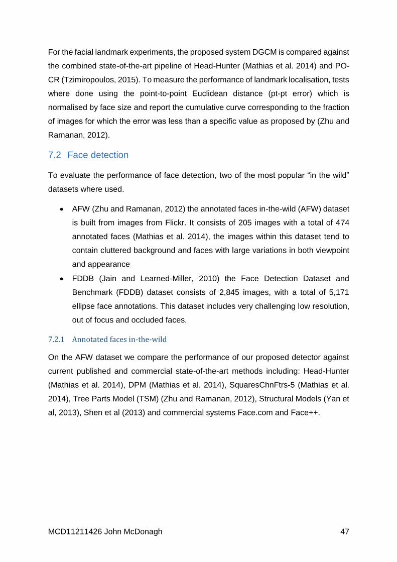
MCD11211426 John McDonagh 47
For the facial landmark experiments, the proposed system DGCM is compared against
the combined state-of-the-art pipeline of Head-Hunter (Mathias et al. 2014) and PO-
CR (Tzimiropoulos, 2015). To measure the performance of landmark localisation, tests
where done using the point-to-point Euclidean distance (pt-pt error) which is
normalised by face size and report the cumulative curve corresponding to the fraction
of images for which the error was less than a specific value as proposed by (Zhu and
Ramanan, 2012).
7.2 Face detection
To evaluate the performance of face detection, two of the most popular “in the wild”
datasets where used.
AFW (Zhu and Ramanan, 2012) the annotated faces in-the-wild (AFW) dataset
is built from images from Flickr. It consists of 205 images with a total of 474
annotated faces (Mathias et al. 2014), the images within this dataset tend to
contain cluttered background and faces with large variations in both viewpoint
and appearance
FDDB (Jain and Learned-Miller, 2010) the Face Detection Dataset and
Benchmark (FDDB) dataset consists of 2,845 images, with a total of 5,171
ellipse face annotations. This dataset includes very challenging low resolution,
out of focus and occluded faces.
7.2.1 Annotated faces in-the-wild
On the AFW dataset we compare the performance of our proposed detector against
current published and commercial state-of-the-art methods including: Head-Hunter
(Mathias et al. 2014), DPM (Mathias et al. 2014), SquaresChnFtrs-5 (Mathias et al.
2014), Tree Parts Model (TSM) (Zhu and Ramanan, 2012), Structural Models (Yan et
al, 2013), Shen et al (2013) and commercial systems Face.com and Face++.
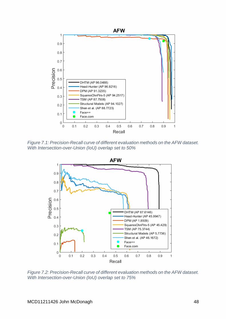
MCD11211426 John McDonagh 48
Figure 7.1: Precision-Recall curve of different evaluation methods on the AFW dataset. With Intersection-over-Union (IoU) overlap set to 50%
Figure 7.2: Precision-Recall curve of different evaluation methods on the AFW dataset. With Intersection-over-Union (IoU) overlap set to 75%

MCD11211426 John McDonagh 49
As illustrated in Figure 7.1, on the AFW dataset with the IoU overlap set to 50%, we
show that our detector is comparable to both current commercial and published state-
of-the-art methods. To further show the accuracy of our proposed detector, we
increased the IoU overlap to 75%, and as can be seen in Figure 7.2, our detector
clearly outperforms all commercial and published methods by a margin of over 10% in
detection accuracy.
7.2.2 Face Detection Dataset and Benchmark
FDDB defines two types of evaluations: the discrete score and continuous score. For
evaluating the discrete score, it counts the number of true positives (detected faces)
against the number of false positives. Detected faces are only considered as true
positive if the IoU ratio to the ground truth ellipse exceeds 0.5. In the continuous score
evaluation, it evaluates the accuracy of the detected bounding ellipse against the
ground truth ellipse, by using the IoU ratio as the matching metric.
Figure 7.3: FDDB Discrete scores.
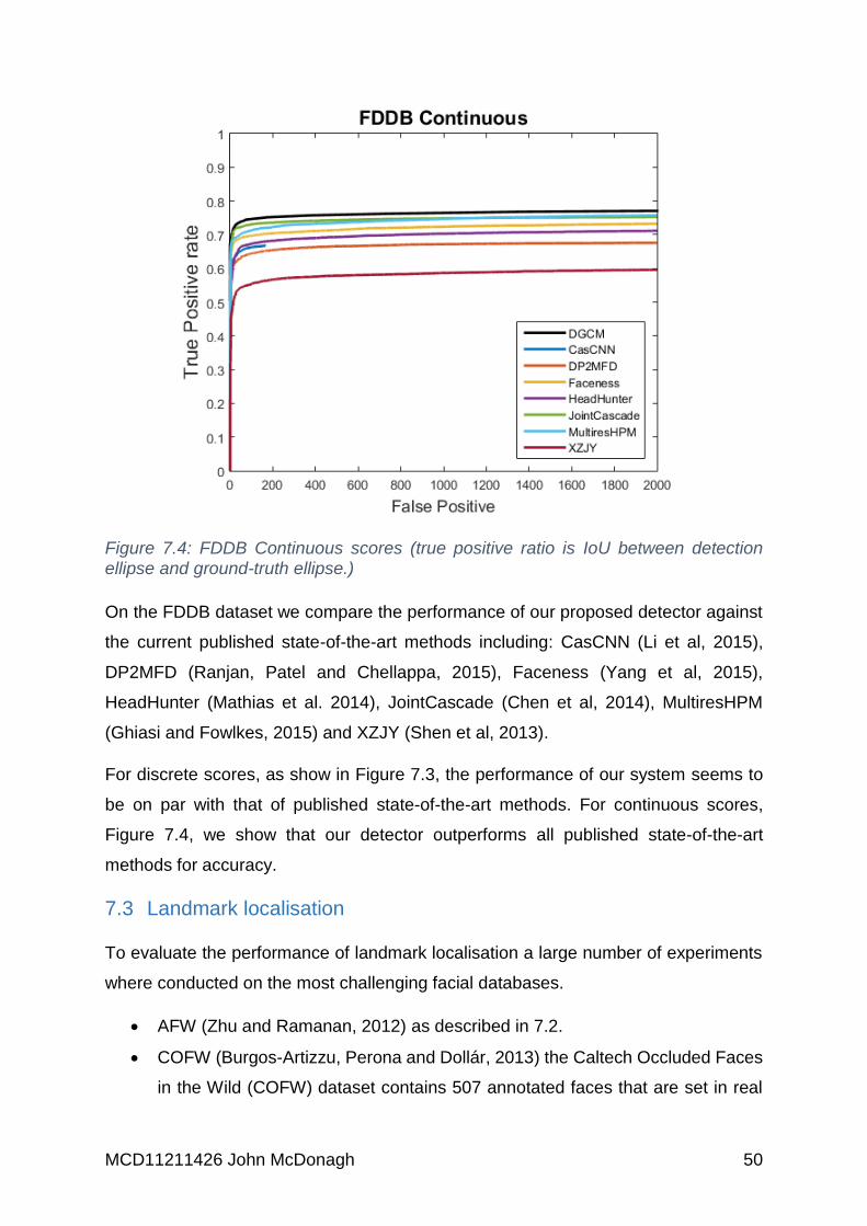
MCD11211426 John McDonagh 50
Figure 7.4: FDDB Continuous scores (true positive ratio is IoU between detection ellipse and ground-truth ellipse.)
On the FDDB dataset we compare the performance of our proposed detector against
the current published state-of-the-art methods including: CasCNN (Li et al, 2015),
DP2MFD (Ranjan, Patel and Chellappa, 2015), Faceness (Yang et al, 2015),
HeadHunter (Mathias et al. 2014), JointCascade (Chen et al, 2014), MultiresHPM
(Ghiasi and Fowlkes, 2015) and XZJY (Shen et al, 2013).
For discrete scores, as show in Figure 7.3, the performance of our system seems to
be on par with that of published state-of-the-art methods. For continuous scores,
Figure 7.4, we show that our detector outperforms all published state-of-the-art
methods for accuracy.
7.3 Landmark localisation
To evaluate the performance of landmark localisation a large number of experiments
where conducted on the most challenging facial databases.
AFW (Zhu and Ramanan, 2012) as described in 7.2.
COFW (Burgos-Artizzu, Perona and Dollár, 2013) the Caltech Occluded Faces
in the Wild (COFW) dataset contains 507 annotated faces that are set in real

MCD11211426 John McDonagh 51
world conditions. The faces tend to have large variations due to pose and
expression, and over 23% of faces have various degrees of occlusion.
Figure 7.5: Accumulated point-to-point error, relative to size of face, for 474 annotated faces from the AFW dataset.
Figure 7.6: Accumulated point-to-point error, relative to size of face, for 507 annotated faces from the COFW dataset.
For landmark localisation, as can be seen in Figure 7.5, the proposed system of this
thesis, DGCM, shows comparable performance to that of the state-of-the-art pipeline
of Head-Hunter (Mathias et al. 2014) and PO-CR (Tzimiropoulos, 2015) on the AFW

MCD11211426 John McDonagh 52
dataset. Also, Figure 7.6 clearly shows that DGCM outperforms the combined pipeline
of Head-Hunter and PO-CR by approximately 20% on the COFW dataset. This is
because of the inaccuracies of head-hunter’s face detector, which makes it a lot harder
for the PO-CR fitting algorithm to fit to occluded faces.
7.4 Execution times
All experiments were done on a 640*480 VGA image from the AFW dataset
(2844520516.jpg). The image pyramid was calculated using the formula
𝑐𝑒𝑖𝑙((1 1.1𝑠𝑐𝑎𝑙𝑒⁄ ) ∗ 𝑖𝑚𝑎𝑔𝑒𝑆𝑖𝑧𝑒) and a step size of 10 pixels was used.
Scale factor
Grid size Initial number of windows
Frontal Time ms
Right Profile Time ms
Left Profile Time ms
2.14 138 x 103 14214 96.092201 81.077698 71.068100
1.95 125 x 94 11750 79.075699 68.065300 60.057598
1.77 114 x 86 9804 72.069099 59.056801 57.054901
1.61 104 x 78 8112 64.061401 48.046101 50.048000
1.46 94 x 71 6674 55.053101 41.039101 43.041000
1.33 86 x 64 5504 45.043098 34.032600 37.035702
1.21 78 x 59 4602 39.037201 32.030701 37.035801
1.10 71 x 53 3763 36.034599 32.030701 34.032398
1.00 64 x 48 3072 32.030899 27.025900 29.028099
0.91 59 x 44 2596 31.029499 27.025900 27.025299
0.83 53 x 40 2120 26.025200 23.022100 22.021400
0.75 49 x 37 1813 27.025700 24.023001 20.019199
0.68 44 x 33 1452 24.023199 20.019400 17.016300
0.62 40 x 30 1200 21.019899 17.016100 15.014400
0.56 37 x 28 1036 19.018299 16.015400 14.013200
0.51 33 x 25 825 16.015301 13.012700 13.012500
0.47 30 x 23 690 10.009600 14.013200 13.012400
0.42 28 x 21 588 13.012500 13.012700 8.008000
0.39 25 x 19 475 14.013400 14.013200 8.007400
0.35 23 x 17 391 13.012200 13.012700 8.007700
Total execution time in ms 732.702095 616.591304 583.559397
Table 7.1: Scaling factors and resulting grid dimensions of a VGA image, with execution times for frontal, right profile and left profile models measured in milliseconds
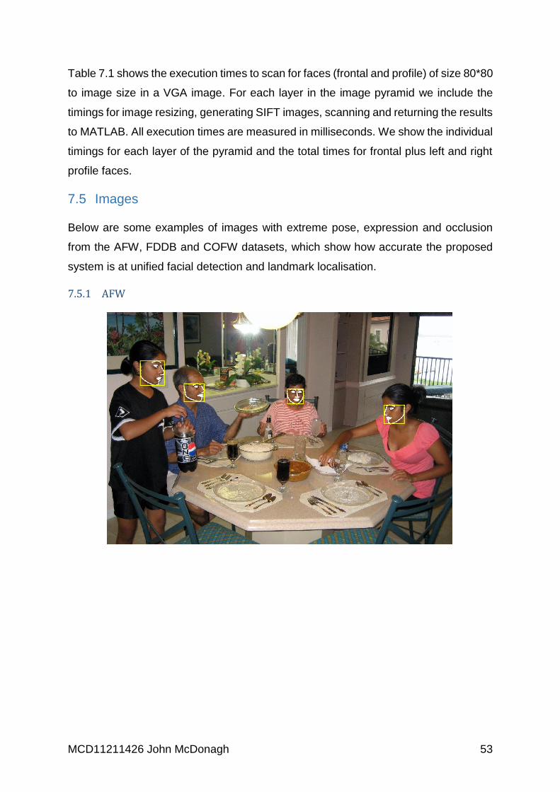
MCD11211426 John McDonagh 53
Table 7.1 shows the execution times to scan for faces (frontal and profile) of size 80*80
to image size in a VGA image. For each layer in the image pyramid we include the
timings for image resizing, generating SIFT images, scanning and returning the results
to MATLAB. All execution times are measured in milliseconds. We show the individual
timings for each layer of the pyramid and the total times for frontal plus left and right
profile faces.
7.5 Images
Below are some examples of images with extreme pose, expression and occlusion
from the AFW, FDDB and COFW datasets, which show how accurate the proposed
system is at unified facial detection and landmark localisation.
7.5.1 AFW

MCD11211426 John McDonagh 54

MCD11211426 John McDonagh 55
7.5.2 FDDB
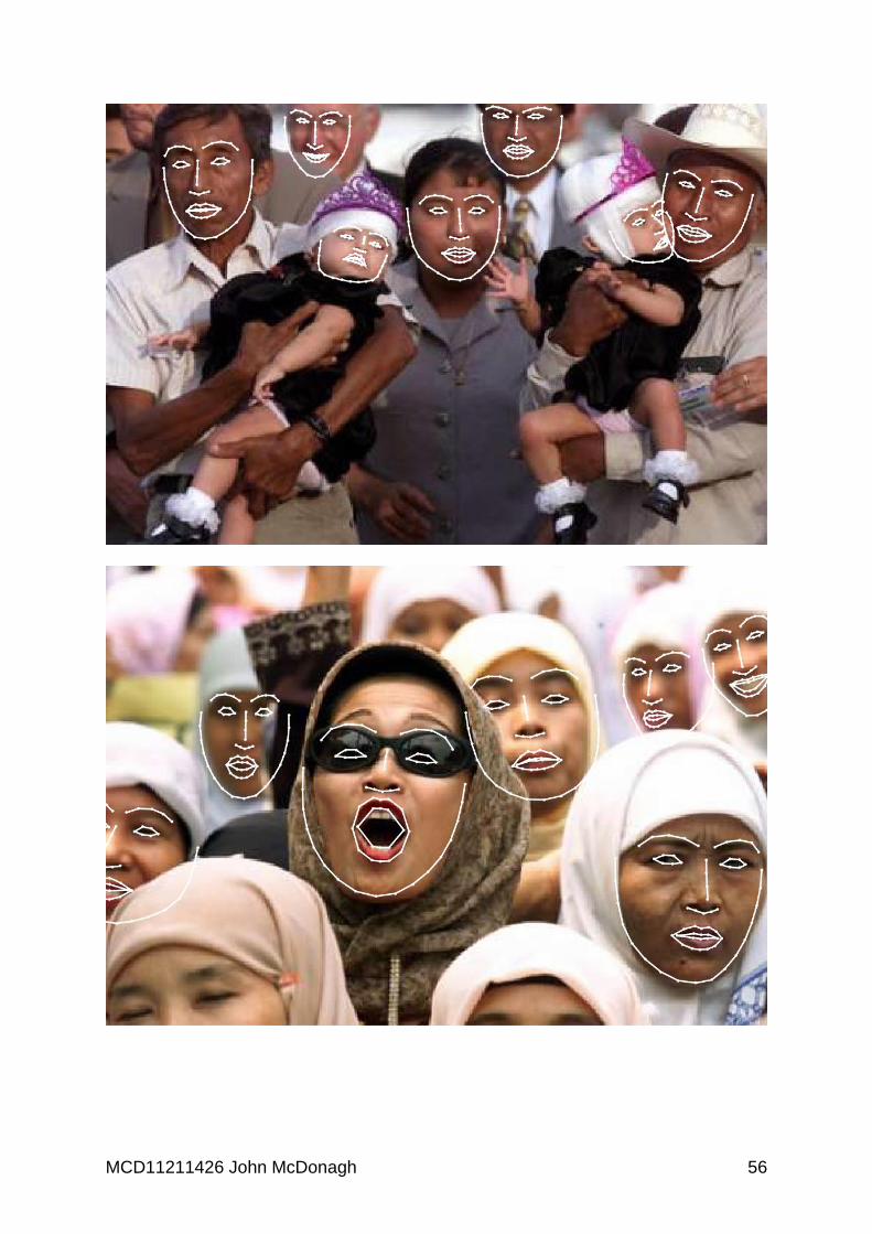
MCD11211426 John McDonagh 56

MCD11211426 John McDonagh 57
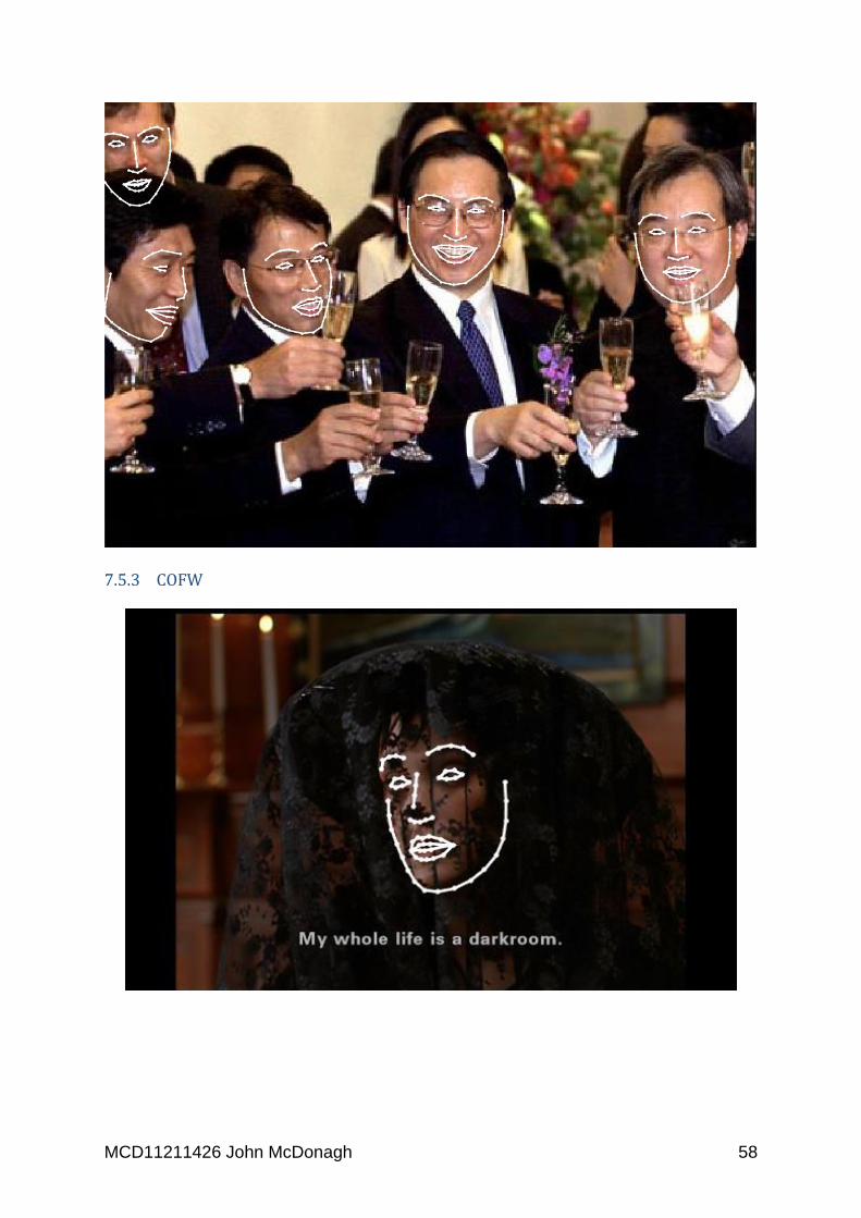
MCD11211426 John McDonagh 58
7.5.3 COFW

MCD11211426 John McDonagh 59

MCD11211426 John McDonagh 60
8 Conclusion
This thesis proposes a novel approach to face detection and landmark localisation
which is termed the Deformable Global Consensus Model (DGCM). DGCM is largely
motivated by the efficiency and robustness of recent Cascaded Regression (CR)
methodologies in facial alignment. But, whereas standard approaches use a face
detector to initialise them, the proposed system of this thesis instead, utilises them in
a parallel fashion, order to detect the location of faces in an arbitrary image.
We report comparable performance to that of published state-of-the-art face detection
algorithms, but as can be seen in Figure 7.2, Figure 7.4 and Figure 7.6 we also show
that the proposed system also detects faces with a higher degree of accuracy. We
also report significant improvement over the standard face detection/landmark
localisation pipeline when performance is measured in terms of landmark localisation.
We also demonstrate that real-time scanning of an arbitrary VGA image can be
achieved as long as the face size is known in advance, Table 7.1.
Figure 8.1: FDDB dataset. Example of low resolution missed faces. Yellow ellipses show faces that are detected, and red ellipses show faces that are not detected
Even though the proposed system is more accurate than current state-of-the-art
systems, it is still not without its problems. One of the main problems was that PO-CR
was trained with just two high resolution models, one model for frontal and another for
profile faces. As can be seen in Figure 8.1, this lead to a lot of missed detections in
the FDDB dataset. Having a second low resolution model trained for both frontal and
profile faces should rectify this problem.

MCD11211426 John McDonagh 61
9 Reference
Al-Shehri, S. A., 2004. A Simple and Novel Method for Skin Detection and Face
Locating and Tracking [pdf] Springer. Available at:
http://link.springer.com/chapter/10.1007%2F978-3-540-27795-8_1 [Accessed on 17
January 2016].
AnandTech, 2015. NVIDIA Posts 350.05 Hotfix Driver – Fixes Games & adds OpenCL
1.2 Support. [online] Available at: http://www.anandtech.com/show/9139/nvidia-posts-
35005-hotfix-driver-fixes-games-adds-opencl-12-support [Accessed 25 June 2015].
Asthana, A., Saragih, J., Wagner, M. and Goecke, R., 2009. Evaluating AAM fitting
methods for facial expression recognition. ACII, pp.1–8.
Belhumeur, P., Jacobs, D., Kriegman, D, and Kumar, N., 2011. Localizing parts of
faces using a consensus of exemplars. CVPR, pp.545-552.
Bernabé, G., Guerrero, G. and Fernández, J., 2012. CUDA and OpenCL
Implementations of 3D Fast Wavelet Transform. [pdf] Available at:
http://ditec.um.es/caps/pdfs/bernabe_lascas12.pdf [Accessed 26 June 2015].
Brown, M. and Lowe, D.G., 2002. Invariant Features from Interest Point Groups. [pdf]
British Machine Vision Conference. Available at:
http://www.comp.leeds.ac.uk/bmvc2008/proceedings/2002/papers/92/full_92.pdf
[Accessed 19 June 2015].
Burgos-Artizzu, X.P., Perona, P. and Dollár, P., 2013. Robust face landmark
estimation under occlusion. ICCV, pp.1513-1520.
Cao, X., Wei, Y., Wen, F. and Sun. J., 2012. Face alignment by explicit shape
regression. IJCV, 107(2), p.177-190
Chang, C.-C. and Lin, C.-J., 2011. LIBSVM: a library for support vector machines.
ACM Transactions on Intelligent Systems and Technology. 2(3) p.27:1==27:27
Chen, D., Cao, X., Wen, F. and Sun, J., 2013. Blessing of dimensionality: High-
dimensional feature and its efficient compression for face verification. CVPR,
pp.3025–3032.

MCD11211426 John McDonagh 62
Chen, D., Ren, S., Wei, Y., Cao, X., and Sun. J., 2014. Joint cascade face detection
and alignment. ECCV, 8694, pp.109-122.
Chew, S.W., Lucey, P., Lucey, S., Saragih, J., Cohn, J.F., Matthews, I. and Sridharan,
S., 2012. In the pursuit of effective affective computing: The relationship between
features and registration. IEEE SMC-B, 42(4), pp.1006-1016.
Cootes, T. F., Edwards, G. J. and Taylor, C. J., 1998. Active appearance models.
Proceedings of the European Conference on Computer Vision, vol. 2, pp.484–498.
Cootes, T., Edwards, E., and Taylor, C., 2001. Active appearance models. TPAMI,
23(6), pp.681–685.
Cootes, T. F., Edwards, G. J. and Taylor, C. J., 2001. Active appearance models.
Pattern Analysis and Machine Intelligence, IEEE Transactions 23(6), pp.681-685.
Cootes, T. F. and Taylor, C. J., 1992. Active shape models — ‘Smart Snakes’.
BMVC92, pp.266-275.
Cristinacce, D. and Cootes, T., 2006. Feature detection and tracking with constrained
local models. [pdf] University of Manchester. Available at:
http://personalpages.manchester.ac.uk/staff/timothy.f.cootes/papers/BMVC06/cristin
acce_bmvc06.pdf [Accessed on 2 October 2015].
Dollar, P., Welinder, P. and Perona, P., 2010. Cascaded pose regression. [pdf]
Available at: http://vision.ucsd.edu/~pdollar/files/papers/DollarCVPR10pose.pdf
[Accessed on 2 December 2015].
Everingham, M., Van Gool, L., Williams, C.K.I., Winn, J. and Zisserman, A., 2009. The
PASCAL Visual Object Classes (VOC) Challenge. [pdf] Available at:
http://homepages.inf.ed.ac.uk/ckiw/postscript/ijcv_voc09.pdf [Accessed on 20
January 2016].
Fang, J., Varbanescu, A. L. and Sips, H., 2011. A Comprehensive Performance
Comparison of CUDA and OpenCL. Parallel Processing (ICPP), International
Conference. IEEE, pp.216-225
Farber, R., 2012. CUDA application design and development. Waltham:Morgan
Kaufmann.
MCD11211426 John McDonagh 63
Felzenszwalb, P.F., Girshick, R.B., McAllester, D. and Ramanan, D., 2010. Object
Detection with Discriminatively Trained Part Based Models [pdf] Available at:
https://www.cs.berkeley.edu/~rbg/papers/Object-Detection-with-Discriminatively-
Trained-Part-Based-Models--Felzenszwalb-Girshick-McAllester-Ramanan.pdf
[Accessed on 12 December 2015].
Getreuer, P., 2010. Colorspace Transformations [online] MATLAB Central. Available
at: http://uk.mathworks.com/matlabcentral/fileexchange/28790-colorspace-
transformations [Accessed on 1 November 2015].
Ghiasi, G. and Fowlkes, C.C., 2014. Occlusion coherence: Detecting and localizing
occluded faces. [online] Cornell University Library. Available at:
http://arxiv.org/abs/1506.08347 [Accessed 30 November 2015].
Gil, L., 2013. A Short introduction to descriptors [blog post] Available at:
https://gilscvblog.wordpress.com/2013/08/18/a-short-introduction-to-descriptors/
[Accessed on 15 June 2015].
Hager, G. and Belhumeur, P., 1998. Efficient region tracking with parametric models
of geometry and illumination. IEEE Transactions on Pattern Analysis and Machine
Intelligence, vol. 20 (10), 1025–1039
Harris, M., 2013. CUDA Pro Tip: Write Flexible Kernels with Grid-Stride Loops [online]
available at: http://devblogs.nvidia.com/parallelforall/cuda-pro-tip-write-flexible-
kernels-grid-stride-loops/ [Accessed on 18 May 2015].
Harris, C. and Stephens, M., 1988. A combined corner and edge detector [pdf].
Proceedings of the 4th Alvey Vision Conference, pp.147–151. Available at:
http://www.bmva.org/bmvc/1988/avc-88-023.pdf [Accessed 19 June 2015].
Huang, C., Ai, H., Li, Y. and Lao, S., 2007. High-Performance Rotation Invariant
Multiview Face Detection. [pdf] IEEE Transactions ON PATTERN ANALYSIS AND
MACHINE INTELLIGENCE. Available at:
http://media.cs.tsinghua.edu.cn/~imagevision/papers/[2007][pami]High%20Performa
nce%20Rotation%20Invariant%20Multi-View%20Face%20Detection%20i0671.pdf
[Accessed 30 June 2015].
MCD11211426 John McDonagh 64
Huang, C., Ai, H., Li, Y. and Lao, S., 2005. Vector Boosting for Rotation Invariant
Multi-View Face Detection [pdf] Available at:
http://lear.inrialpes.fr/people/triggs/student/vj/huang-iccv05.pdf [Accessed on 30
June 2015].
Impact Research Group, (2015) Parboil Benchmarks [online] University of Illinois.
Available at: http://impact.crhc.illinois.edu/Parboil/parboil.aspx [Accessed 27 June
2015].
Karimi, K., Dickson, N. G. and Hamze, F., 2010. A Performance Comparison of CUDA
and OpenCL. [online] Cornell University Library. Available at:
http://arxiv.org/abs/1005.2581 [Accessed 24 June 2015].
Komatsu, K., Sato, K., Arai, Y., Koyama, K., Takizawa, H. and Kobayashi, H., 2010.
Evaluating Performance and Portability of OpenCL Programs. [pdf] The Fifth
International Workshop on Automatic Performance Tuning. Available at:
http://citeseerx.ist.psu.edu/viewdoc/download?doi=10.1.1.456.5743&rep=rep1&type
=pdf [Accessed 24 June 2015].
Li, H., Lin, Z., Shen, X., Brandt, J. and Hua, G., 2015. A Convolutional Neural Network
Cascade for Face Detection. [pdf] Available at:
http://personal.stevens.edu/~hli18/papers/CVPR2015_CasCNN.pdf [Accessed on 17
January 2016].
Lowe, D. G., 1999. Object Recognition from Local Scale-Invariant Features. [pdf]
Available at: http://www.cs.ubc.ca/~lowe/papers/iccv99.pdf [Accessed on 15 October
2015].
Lowe, D. G., 2004. Distinctive Image Features from Scale-Invariant Keypoints.
International Journal of Computer Vision 60(2) pp.91-110.
Lucas, B. and Kanade, T., 1981. An iterative image registration technique with an
application to stereo vision. [pdf] Stanford. Available at:
http://graphics.stanford.edu/courses/cs448a-00fall/lucaskanade81.pdf [Accessed on
11 November 2015].
Lucey, S., Wang, Y., Cox, M., Sridharan, S. and Cohna, J. F., 2009. Efficient
Constrained Local Model Fitting for Non-Rigid Face Alignment [online] NCBI. Available
MCD11211426 John McDonagh 65
at: http://www.ncbi.nlm.nih.gov/pmc/articles/PMC2799037/ [Accessed on 27
December 2015].
Luitjens, J., 2014. Faster Parallel Reductions on Kepler [online] NVIDIA. Available at:
http://devblogs.nvidia.com/parallelforall/faster-parallel-reductions-kepler/ [Accessed
on 10 October 2015].
Mathias, M., Benenson, R., Pedersoli, M. and Van Gool, L., 2014. Face detection
without bells and whistles. ECCV. 8692, pp.720-735.
Matthews, I. and Baker, S., 2004. Active appearance models revisited. IJCV, 60(2),
pp.135–164.
NVIDIA, 2012. NVIDIA’s Next Generation CUDATM Compute Architecture: KeplerTM
GK110, Whitepaper. [pdf] NVIDIA. Available at:
http://www.nvidia.co.uk/content/PDF/kepler/NVIDIA-Kepler-GK110-Architecture-
Whitepaper.pdf [Accessed 20 November 2015].
NVIDIA, 2016. CUDA Toolkit Archive. [online] NVIDIA Available at:
https://developer.nvidia.com/cuda-toolkit-archive [Accessed 8 January 2016].
NVIDIA developer zone, 2015. CUDA toolkit documentation. [online] NVIDIA.
Available at: http://docs.nvidia.com/cuda/cuda-c-programming-
guide/#axzz3eAOkWhLD [Accessed 20 June 2015].
PASCAL, 2005. The Pascal object recognition database collection. [online] University
of Southampton. Available at: http://www.pascalnetwork.org/challenges/VOC/
[Accessed 20 June 2015].
Ranjan, R., Patel, V. M. and Chellappa, R., 2015. A Deep Pyramid Deformable Part
Model for Face Detection. [pdf] Cornell University Library. Available at:
http://arxiv.org/pdf/1508.04389v1.pdf [Accessed on 17 January 2016].
Saragih, J., Lucey, S. and Cohn, J., 2011. Deformable model fitting by regularized
landmark mean-shift. IJCV, 91(2), pp.200-215.
Shen, X., Lin, Z., Brandt, J. and Wuk, Y., 2013. Detecting and aligning faces in image
retrieval. CVPR, pp.3460-3467.

MCD11211426 John McDonagh 66
Tzimiropoulos, G., 2015. Project-Out Cascaded Regression with an application to
Face Alignment. CVPR, pp.3659-3667.
Viola, P. and Jones, M. J., 2003. Fast Multi-view Face Detection [pdf] Available at:
http://citeseerx.ist.psu.edu/viewdoc/download?doi=10.1.1.145.7598&rep=rep1&type
=pdf [Accessed 1 July 2015].
Viola, P. and Jones, M. J., 2004. Robust Real-Time Face Detection. [pdf] International
Journal of Computer Vision. Available at: http://www.vision.caltech.edu/html-
files/EE148-2005-Spring/pprs/viola04ijcv.pdf [Accessed 29 June 2015].
Wales Online, 2015. Selfies and a pint as Barbarians squad get together [image
online] Available at: http://www.walesonline.co.uk/sport/rugby/rugby-news/wales-
internationals-adam-jones-alex-9332896 [Accessed on 10 January 2016].
Wang, N., Gao, X., Tao, D. and Li, X., 2014. Facial Feature Point Detection: A
Comprehensive Survey [pdf] Available at: http://arxiv.org/pdf/1410.1037.pdf
[Accessed on 24 December 2015].
Yan, J., Zhang, X., Lei, Z. and Li, S., 2013. Face detection by structural models.
Image and Vision Computing. 32(10), pp.790-799.
Yang, S., Luo, P., Loy, C.C. and Tang, X., 2015. From Facial Parts Responses to Face
Detection: A Deep Learning Approach. [pdf] Cornell University Library. Available at:
http://arxiv.org/pdf/1509.06451v1.pdf [Accessed on 17 January 2016].
Zhu, X. and Ramanan, D., 2012. Face detection, pose estimation, and landmark
estimation in the wild. CVPR, pp.2879–2886.
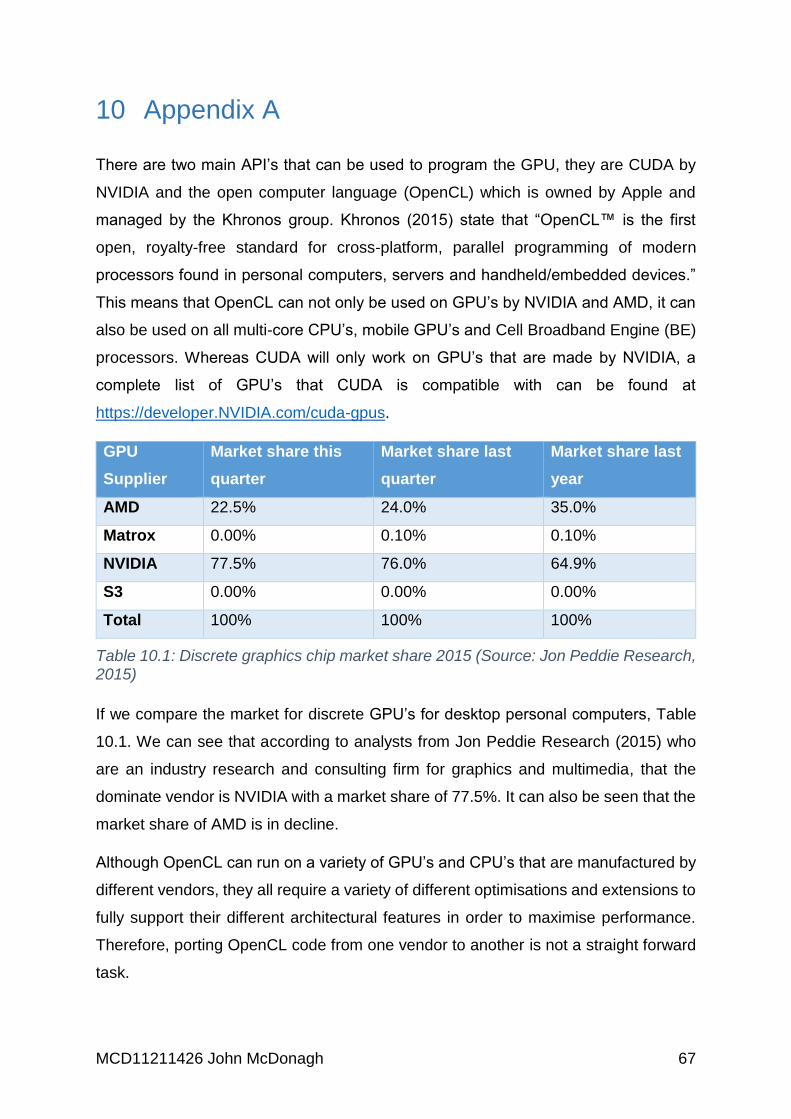
MCD11211426 John McDonagh 67
10 Appendix A
There are two main API’s that can be used to program the GPU, they are CUDA by
NVIDIA and the open computer language (OpenCL) which is owned by Apple and
managed by the Khronos group. Khronos (2015) state that “OpenCL™ is the first
open, royalty-free standard for cross-platform, parallel programming of modern
processors found in personal computers, servers and handheld/embedded devices.”
This means that OpenCL can not only be used on GPU’s by NVIDIA and AMD, it can
also be used on all multi-core CPU’s, mobile GPU’s and Cell Broadband Engine (BE)
processors. Whereas CUDA will only work on GPU’s that are made by NVIDIA, a
complete list of GPU’s that CUDA is compatible with can be found at
https://developer.NVIDIA.com/cuda-gpus.
GPU
Supplier
Market share this
quarter
Market share last
quarter
Market share last
year
AMD 22.5% 24.0% 35.0%
Matrox 0.00% 0.10% 0.10%
NVIDIA 77.5% 76.0% 64.9%
S3 0.00% 0.00% 0.00%
Total 100% 100% 100%
Table 10.1: Discrete graphics chip market share 2015 (Source: Jon Peddie Research, 2015)
If we compare the market for discrete GPU’s for desktop personal computers, Table
10.1. We can see that according to analysts from Jon Peddie Research (2015) who
are an industry research and consulting firm for graphics and multimedia, that the
dominate vendor is NVIDIA with a market share of 77.5%. It can also be seen that the
market share of AMD is in decline.
Although OpenCL can run on a variety of GPU’s and CPU’s that are manufactured by
different vendors, they all require a variety of different optimisations and extensions to
fully support their different architectural features in order to maximise performance.
Therefore, porting OpenCL code from one vendor to another is not a straight forward
task.
MCD11211426 John McDonagh 68
10.1 CUDA and OpenCL Performance comparison
A fair comparison between CUDA and OpenCL can only be achieved on an NVIDIA
graphics card as CUDA is not compatible with any other vendor. But, this is not
currently possible, as NVIDIA has not implemented OpenCL 2.0 into their driver set. It
was reported by AnandTech (2015) that NVIDIA have only just recently added support
for OpenCL 1.2 into their driver release, version 350.05 on April 2015. Therefore, this
thesis will summarise the results of recent performance comparisons from peer
reviewed published papers.
Research undertaken by (Karimi et al, 2010) into the performance comparison
between CUDA and OpenCL in data transfer to and from the GPU, kernel execution
and end-to-end application running times, was done by implementing a Monte Carlo
simulation of a quantum spin system with quantum bit (qubits) sizes ranging from 8 to
128. This was accomplished using an NVIDIA GeForce GTX-260 GPU. To profile the
application, they split it into six stages
1. Setup GPU
2. Read input
3. Copy data to GPU
4. Execute kernel on the GPU
5. Copy data beck to the host
6. Process returned data on CPU and output results
Table 10.2 summarise of the results that they achieved and is broken down into 3
parts. Kernel Running Time (step 4), Data Transfer Time (steps 3 and 5) and End-To-
End Running time (steps 1-6).
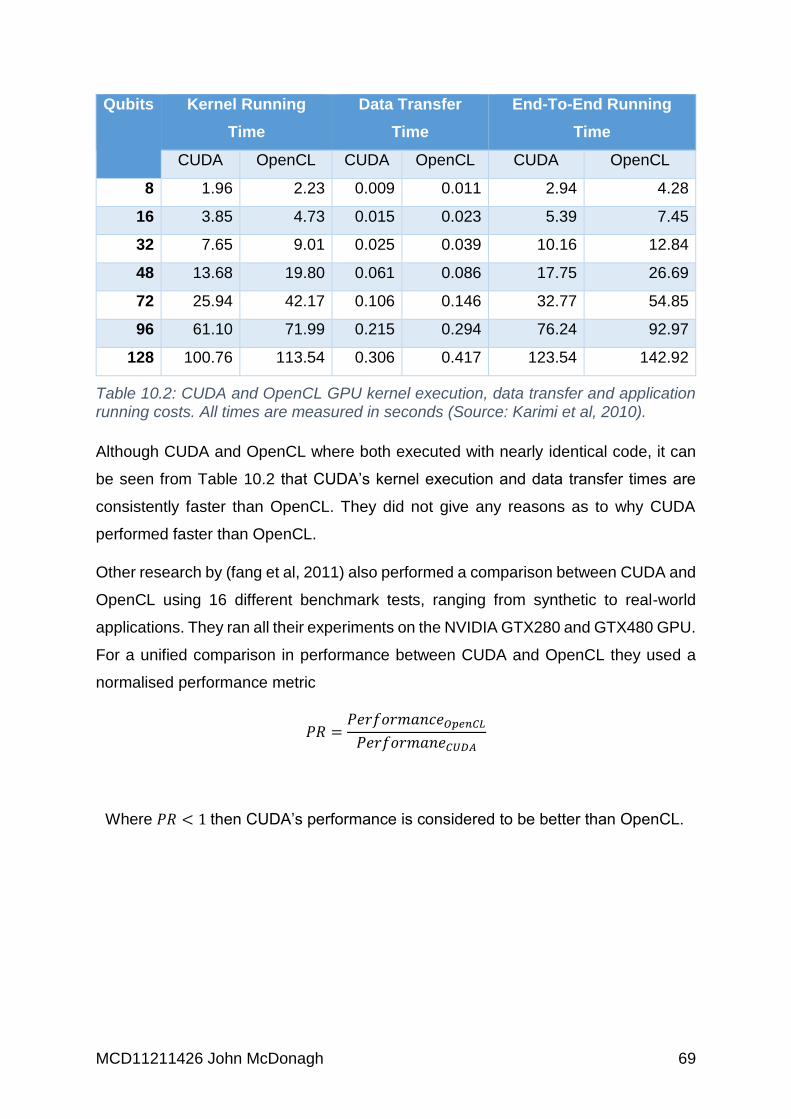
MCD11211426 John McDonagh 69
Qubits Kernel Running
Time
Data Transfer
Time
End-To-End Running
Time
CUDA OpenCL CUDA OpenCL CUDA OpenCL
8 1.96 2.23 0.009 0.011 2.94 4.28
16 3.85 4.73 0.015 0.023 5.39 7.45
32 7.65 9.01 0.025 0.039 10.16 12.84
48 13.68 19.80 0.061 0.086 17.75 26.69
72 25.94 42.17 0.106 0.146 32.77 54.85
96 61.10 71.99 0.215 0.294 76.24 92.97
128 100.76 113.54 0.306 0.417 123.54 142.92
Table 10.2: CUDA and OpenCL GPU kernel execution, data transfer and application running costs. All times are measured in seconds (Source: Karimi et al, 2010).
Although CUDA and OpenCL where both executed with nearly identical code, it can
be seen from Table 10.2 that CUDA’s kernel execution and data transfer times are
consistently faster than OpenCL. They did not give any reasons as to why CUDA
performed faster than OpenCL.
Other research by (fang et al, 2011) also performed a comparison between CUDA and
OpenCL using 16 different benchmark tests, ranging from synthetic to real-world
applications. They ran all their experiments on the NVIDIA GTX280 and GTX480 GPU.
For a unified comparison in performance between CUDA and OpenCL they used a
normalised performance metric
𝑃𝑅 =𝑃𝑒𝑟𝑓𝑜𝑟𝑚𝑎𝑛𝑐𝑒𝑂𝑝𝑒𝑛𝐶𝐿
𝑃𝑒𝑟𝑓𝑜𝑟𝑚𝑎𝑛𝑒𝐶𝑈𝐷𝐴
Where 𝑃𝑅 < 1 then CUDA’s performance is considered to be better than OpenCL.
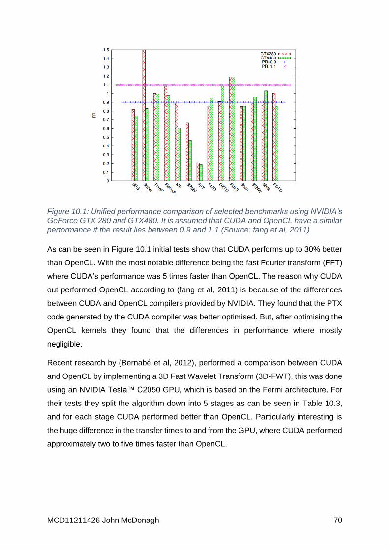
MCD11211426 John McDonagh 70
Figure 10.1: Unified performance comparison of selected benchmarks using NVIDIA’s GeForce GTX 280 and GTX480. It is assumed that CUDA and OpenCL have a similar performance if the result lies between 0.9 and 1.1 (Source: fang et al, 2011)
As can be seen in Figure 10.1 initial tests show that CUDA performs up to 30% better
than OpenCL. With the most notable difference being the fast Fourier transform (FFT)
where CUDA’s performance was 5 times faster than OpenCL. The reason why CUDA
out performed OpenCL according to (fang et al, 2011) is because of the differences
between CUDA and OpenCL compilers provided by NVIDIA. They found that the PTX
code generated by the CUDA compiler was better optimised. But, after optimising the
OpenCL kernels they found that the differences in performance where mostly
negligible.
Recent research by (Bernabé et al, 2012), performed a comparison between CUDA
and OpenCL by implementing a 3D Fast Wavelet Transform (3D-FWT), this was done
using an NVIDIA Tesla™ C2050 GPU, which is based on the Fermi architecture. For
their tests they split the algorithm down into 5 stages as can be seen in Table 10.3,
and for each stage CUDA performed better than OpenCL. Particularly interesting is
the huge difference in the transfer times to and from the GPU, where CUDA performed
approximately two to five times faster than OpenCL.

MCD11211426 John McDonagh 71
3D-FWT
Frame size
512x512 1Kx1K 2Kx2K
CUDA OpenCL CUDA OpenCL CUDA OpenCL
1. CPU to GPU transfer 11.62 25.19 45.6 86.38 181.63 325.52
2. 1D-FWT on frames 2.11 3.53 4.18 6.64 7.73 11.73
3. 1D-FWT on rows 2.37 3.85 2.39 5.89 2.39 6.97
4. 1D-FWT on cols 2.29 3.80 6.86 9.82 25.15 29.29
5. GPU to CPU transfer 10.82 50.75 41.58 167.66 164.68 637.96
Table 10.3: CUDA and OpenCL execution times for a tiled 3D-FWT implementation on an input video containing 64 frames of increasing sizes. All times are measured in milliseconds. (Source: Bernabé et al, 2012).
The reason for this according to (Bernabé et al, 2012), is because OpenCL has a large
environmental setup overhead, and that the huge discrepancy in transfer times is
because OpenCL is designed for general compute devices.
Other research conducted by (Komatsu et al, 2010) was done where they selected
two programs from the NVIDIA GPU Computing SDK 3.0, a bandwidth test and matrix
multiply, plus three CUDA programs from the parboil benchmark suite (The Impact
Research Group, 2015), Coulombic Potential (CP), Magnetic Resonance Imaging Q
(MRI-Q), and Magnetic Resonance Imaging FHD (MRI-FHD). They ported the CUDA
code from these programs to OpenCL as faithfully as possible, by only changing
syntax/API calls where needed.
In their initial tests using a NVIDIA Tesla C1060 GPU. Figure 10.2, showed that CUDA
ran all the algorithms several times faster than OpenCL, with the exception of the
bandwidth test which was near identical in speed.
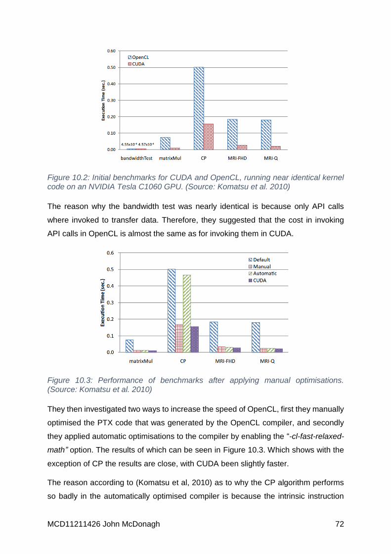
MCD11211426 John McDonagh 72
Figure 10.2: Initial benchmarks for CUDA and OpenCL, running near identical kernel code on an NVIDIA Tesla C1060 GPU. (Source: Komatsu et al. 2010)
The reason why the bandwidth test was nearly identical is because only API calls
where invoked to transfer data. Therefore, they suggested that the cost in invoking
API calls in OpenCL is almost the same as for invoking them in CUDA.
Figure 10.3: Performance of benchmarks after applying manual optimisations. (Source: Komatsu et al. 2010)
They then investigated two ways to increase the speed of OpenCL, first they manually
optimised the PTX code that was generated by the OpenCL compiler, and secondly
they applied automatic optimisations to the compiler by enabling the “-cl-fast-relaxed-
math” option. The results of which can be seen in Figure 10.3. Which shows with the
exception of CP the results are close, with CUDA been slightly faster.
The reason according to (Komatsu et al, 2010) as to why the CP algorithm performs
so badly in the automatically optimised compiler is because the intrinsic instruction
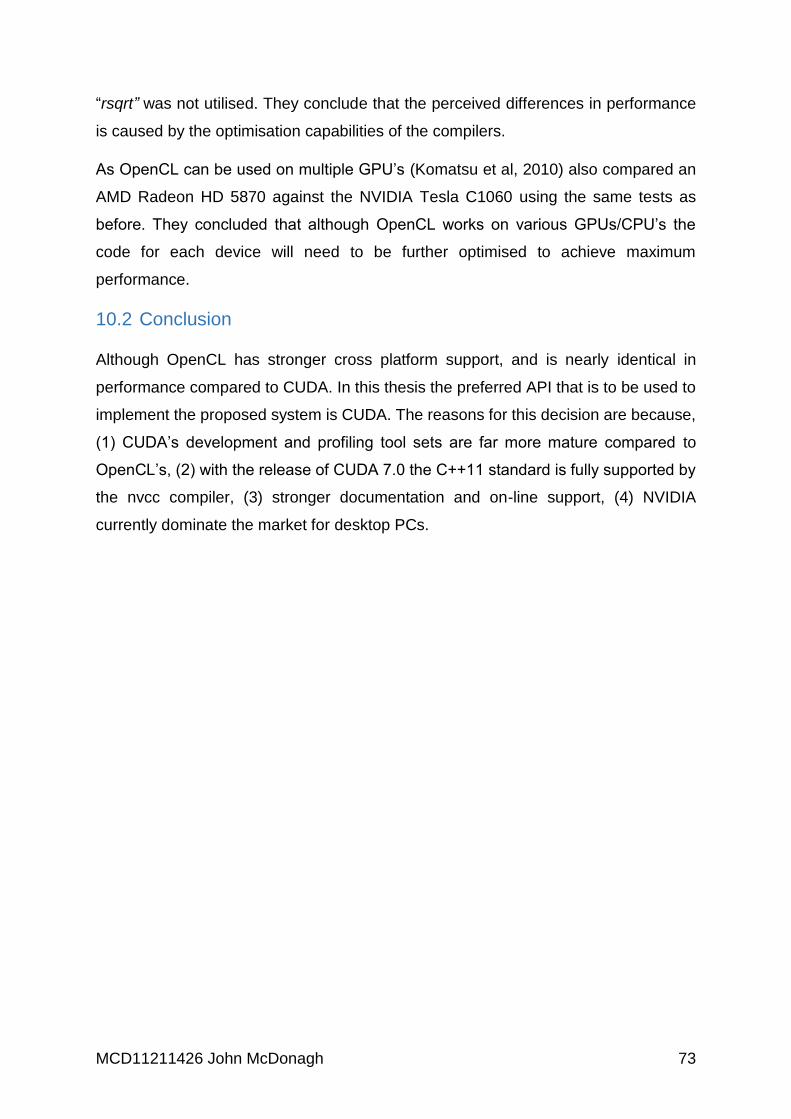
MCD11211426 John McDonagh 73
“rsqrt” was not utilised. They conclude that the perceived differences in performance
is caused by the optimisation capabilities of the compilers.
As OpenCL can be used on multiple GPU’s (Komatsu et al, 2010) also compared an
AMD Radeon HD 5870 against the NVIDIA Tesla C1060 using the same tests as
before. They concluded that although OpenCL works on various GPUs/CPU’s the
code for each device will need to be further optimised to achieve maximum
performance.
10.2 Conclusion
Although OpenCL has stronger cross platform support, and is nearly identical in
performance compared to CUDA. In this thesis the preferred API that is to be used to
implement the proposed system is CUDA. The reasons for this decision are because,
(1) CUDA’s development and profiling tool sets are far more mature compared to
OpenCL’s, (2) with the release of CUDA 7.0 the C++11 standard is fully supported by
the nvcc compiler, (3) stronger documentation and on-line support, (4) NVIDIA
currently dominate the market for desktop PCs.