AD-AL13 040 MARYLAND UNIV COLL90E PARK COMPUTER SCIENCE CENTER FIG 9/2

AN INVESTIGATION OF FUNCTIZONAL CORRECTNESS ISSUES192 00 ULPFG6080) 00

UNCLASSIFIED CSC-TR-1135 AFOSR-TR-82-0263 NLflllfffflllfffIIIIIIIIIIIIIIhfIIIIIIIIIIIIIIffllfllfIIIEIIEIIIIIIEEIIEEIIIIIIIIEEIIIIIIIIIIIIIIlfflfflEIIIEEEIEEI

~ 1111 .0 1 2 .I L.21..8

11111 .25 .I 4 111111.6

"A. MICROCOPY RESOLUTION TEST CHART.NA TIONAL BURLAU Of S TANDARDS 1963 A

.4'14

qt44

1m1A4 b4

joj

Technical Report TR-1135 January, 1982j0 -F49620-80-C001

An Investigation ofFunctional Correctness Issues*

Douglas D. Dunlop

Accession For* NOTIS GRA&V

TIZC TAB -uamo1.nee 0Justtiviation

i atibo -- AIR FORCE OFFTCE 01? SCIENTIFIC RESARCM (AYWS)VOTI CE OF TRANSMI TAL TO DTIC0

Availblt Co- his technic). repor't hns been revievsd and isvail and/o approved for pul-.ii -elesse IAW AFR 19)-12.

pist Special Distribution is unlimited.

fiH D Chiec, 1oohuical Information Division

Dissertation submitted to the Faculty of the Graduate Schoolof the University of Maryland in partial fulfillment

of the requirements for the degree ofDoctor of Philosophy

1982

-----------------------------

*This work was supported in part by the kir Force Office ofScientific Rsearch Contract -F4962080-COO01 to the Univer-sity of Maryland.

-'.

UNCLASSIFIED,V acURT#CLASS1FrICATION 0O7 THIS PAGE (I0.en Date Entrred __________________

REPOT DCUMNTATON AGEREAD INSTRUCTIONSREPOT DCUMNTATON AGEBEFORE COMPLETING FORMI1. 610311T NUM13ER 2.GOVT ACCESSION No. 3. RECIPIENV-S CATALOG NUMBER

.TI TL E (Ofid Subtiti-) b.TYPE OF REPORT & PERIOD COVERED

AN INVESTIGATION OF FUNCTIONAL CORRECTNESS TECHNICAL

ISSUES . ~PERFORMING Fir- REPORT NUMBER

'TR-11357. AUTHOR(s) 1.1S CON TRACT OR GRANT NUMBER(&)

Douglas D. Dunlop . . A 9620--80-C-000l

S. PERFORMING ORGANIZATION NAME AND ADDRESS 10~. PROGRAM ELEMENT PROJECT, TASK

Computer Science Center * R OKUI UBR

University of Maryland :61102F; 2304/A2College Park MD 20742 ______________

It. CONTROLLING OFFICE NAME AND ADDRESS 12. IIEPORT DATE

Mathematical & Information Sciences Directiaftte' JAN 82Air Force Office of Scientific Research 5. NIM;ER OF PAGES

BollineAFBDC__20332 ______________

14. MONITORING AGENCY NAME & ADDRESS(if different from Controfili OI ie) 15SECURITY CLASS. (of this report)

UNCLASSIFIEDIS&. OECLASSIFiCATION.OOWNGRADNG.

SCHEDULE

IS. DISTRIBUTION STATEMENT (of this Report)

Approved for public release; distribution urilimitect,

17. DISTRIBUTION STATEMENT (of the abstract entered in Block 20. it different from. Report)

IS. SUPPLEMENTARY NOTES

IS. KEY WORDS (Continue on reverse aide It necessary and identify by block number)

ABSTRACT (Continue on reverse side It necessary and Identity by bloc.k nvuw)

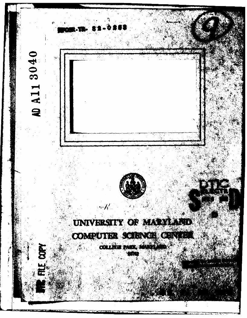
~ V~.Given a program and an abstract functional specification that the program isintended to satisfy, a fundamental question is whether the program executes inaccordance with (i.e. is correct with respect to) the specification. A simple

functional correctness technique is initially defined which is based on primeprogram decomposition of composite programs. This technique is analyzed andthe Oitbb iJffdb the need for each intended loop function and the inflexibility

of the prime program decomposition strategy are discussed. NTh (CONTINUED)

DO 1 pN7 1473 90ITION OF I NOV 5115I OBSOLETE

SECRVCLAI 1AON 1F TIS PACiE who oaf

" UNCLASSIFIEDe, ftlrY LASSIA CATIOM OF TIS PAG;E(M Pat* Rplo,.#)

ITEM #20, CONTINUED: notion of a reduction hOppt"heais is then defined which canbe used in the place of an intended loop function in the verification process.Furthermore, an efficient proof decomposition strateg for composite programs issuggested which is based on a sequence of proof transformations.UA heuristic technique is then proposed for synthesi;ing intended functions for

UWHILE loops in initialized loop programs. Althoughthe technique seems to be* useful in a wide range of commonly occuring aplcaft ons, it is explained that

the heuristic relies on the loop behaving in'k-'re"Onabli' manner. A model of'reasonable' loop behavior, a uniformly impliomt0,*loop, is defined. It is

j shown that, for any uniformly implemented lo6~:Zan'Mnadequate intended loop func-tion may be generalized (i.e. made more descripfve) in a systematic manner.

*StCUMITY CLASINVICATIO11 OF T-1 PA49(fteft DOMA Intrn0

I :

ABSTRACT

Title of Dissertation: AN INVESTIGATION OF FUNCTIONALCORRECTNESS ISSUES

Douglas Dixon Dunlop, Doctor of Philosophy, 1982

Dissertation directed by: Dr. Victor R. EasiliAssociate ProfessorDepartment of Computer Science

Given a program and an abstract functional specificationthat the program is intended to satisfy, a fundamental questionis whether the program executes in accordance with (i.e. iscorrect with respect to) the specification. A simple functionalcorrectness technique is initially defined which is based onprime program decomposition of composite programs. This tech-nique is analyzed and the problems of the need for each intendedloop function and the inflexibility of the prime program decompo-sition strategy are discussed. The notion of a reductionhypothesis is then defined which can be used in the place of anintended loop function in the verification process. Furthermore,an efficient proof decomposition strategy for composite programsis suggested which is based on a sequence of proof transforma-tions.

A heuristic technique is then proposed for synthesizingintended functions for WHILE loops in initialized loop programs.Although the technique seems to be useful in a wide range of com-monly occurring applications, it is explained that the heuristicrelies on the loop behaving in a wreasonable" manner. A model of* reasonable* loop behavior, a uniformly implemented loop, isdefined. It is shown that, for any uniformly implemented loop,an inadequate intended loop function may be generalized (i.e.made more descriptive) in a systematic manner.

Sown=,-

I

ACKNOWLEDGMENTS

I would like to express my thanks to my advisor, Dr. VictorBasili, for the guidance and encouragement he has providedthroughout my course of study at Maryland. Dr. Basili has put inmany long hours making helpful comments on my work and proposingdirections for research which often proved fruitful.

I would like to thank Dr. Harlan Mills for a number of bene-ficial discussions concerning this research effort. To a largeextent, the work in this dissertation is inspired by Dr. Mills'research into the nature of loop computation. I would also liketo thank Dr. Richard Hamlet, Dr. Mark Weiser, Dr. John Gannon,David Barton and Larry Morell for their helpful comments andsuggestions on earlier drafts of the material in this disserta-t ion.

Above all, I am grateful for the constant patience, supportand encouragement provided by my wife, Janet Dunlop.

This work was supported in part by the Air Force Office ofScientific Research Contract AFOSR-F49620-80-C-001 to the Univer-sity of Maryland.

V.I

-I

Table of Contents

2 A Comp~arative Analysis of Functional Correctness ......... 42.1 The Functional Correctness Technique ................ 52.2 The Loop Invariant f(XO) - f(X) ...... 0............. 102.3 Comparing the Hoare and Mills Loop Proof Rules ..... 162.4 Subgoal Induction and Functional Correctness ..... 172. initialized Loops . ... ... .... .... ....... o ... 202.6 Discussion o...........00... ........... 0.00 23

3 A New Verification Strategy For iterative Programs ... .... 24'3.1 Constructing a Reduction Hypothesis ... 00.. 0..00 283.2 Relation to Standard Correctness Techniques ..... 373.3 Proof Transformations o . ... o. . . . .................. 403.4 Discussion ... oo...... oo ........... oo ..... 42

4 A Heuristic For Deriving Loop Functions .......... 444.1 The Technique .................... 45

4.3 Complete Constraints .......................... oo.... 564.4 '*Tricky* Programs ooo................ 604.5 BU and TD Loops .................... 624.6 Related Wo.rk ..................... 684.7 Discussion ...................... 70

5SAnalyzing Uniformly ImplemntedLoops .... .... . 71

5.2 Uniformly ImplementedrLoops ......................... 76

5.4 Simplifying the 'Iteration Condition . ............... 845.5 Recognizing Uniformly Implemented Loops ............. 875.6 Related Work ........................................ 89

6 Summary and Concluding Rmarks ....................... ... 927 References ..........................................*.... 93

i,

List of Figures

Figure 2.1 Derive and Verify Rules .......-........Figure 2.2 The Sets S1-S5 ........................ 13Figure 2.3 Flow Chart Program *........................ 18

1. Introduction

The notion of program correctness is fundamental in softwareengineering and is of increasing importance as computers are usedin more critical applications. Before being released for use,software usually undergoes a validation process, i.e. an act ofreasoning in favor of its correctness. There exist two majorvalidation approaches. The first is testing, and consists ofexecuting the program on a number of inputs and then showing thatthe results are in agreement with the program specification. Thealternative validation technique is program verification (or aproof of program correctness). A program is verified by apply-ing, at some level of formality, logical and mathematical reason-ing concerning the program and specification in order to certifytheir consistency. In this dissertation, we consider the verifi-cation approach to the program validation problem.

Unfortunately, a proof of correctness for any nontrivialprogram is a task that may be fraught with many difficulties.While our research addresses a number of these issues, there areothers which we choose to ignore. For one thing, we assume thatthe program specification has been sufficiently formalized tomake a rigorous proof of correctness possible. In practice, thiscan be a formidable task for programs which are intended to solvecomplex problems. Secondly, we will restrict our attention toprocedureless, sequential, structured programs. We do not con-sider, therefore, the issues involved in proving programs con-taining global/local variables, GOTOs, parameter passing or con-currency.

Although our primary interest in studying verification is asa method of validating programs, research in this field often hasimplications for other areas of software engineering. For onething, a crucial aspect of proving the correctness of a programis the act of readiln and understanding its behavior. Any tech-nique or metodology which facilitates this act is useful notonly as a verification tool, but also as an aid in comprehending,documenting, modifying and maintaining programs. Secondly,verification research can provide insight into what constitutes a

* "good" program. Many practices associated with Ostructured pro-gramming," for example, are aimed at producing programs which canfeasibly be proven correct. It is reasonable to expect thatresearch into program characteristics which influence their veri-fiability should well have significant implications for the pro-gram development process.

Our approach to program verification is based largely on thework in [Mills 72, Mills 751. This methodology has e-ome to beknown as functional correctness and centers around rules for

* proving a prime program (i.e. basic flow chart structure) correctwith respect to a specification which has been formulated as amathematical function. The goal of our research is a thoroughstudy of a number of key issues dealing with the practical

i .

application of the functional correctness methodology.

A straightforward version of functional correctness based on

prime program decomposition of composite programs is defined inChapter 2. This verification strategy is then compared and con-trasted with other standard verification methodologies. In par-ticular, the goal of the study is to analyze the theoreticalrelationships between functional, inductive assertion and subgoal

induction proofs of correctness. In the analysis, it is observedthat the prime program decomposition strategy causes some func-

tional correctness proofs to be somewhat more complex than their

inductive assertion or subgoal induction counterparts.

A primary impediment to applying functional correctness on a

large scale in practice is the requirement that each WHILE loopin the program be tagged with an adequate intended function.Such a function describes the intended input/output behavior ofthe loop over a suitably general input domain. hile supplyingintended functions with program segments is no doubt a good pro-gramming practice, programmers often fail to supply this documen-tation due to the effort and difficulty involved. This is par-ticularly true of intended loop functions (as opposed, for exam-pie, to those for initialized loops) since they tend to be rela-tively complex and difficult to state. Furthermore, most programmaintenance is currently being done on programs with undocumentedintended loop functions. Chapters 3, 4 and 5 deal largely with

,'. the issue of verifying programs which contain WHILE loops withmissing or inadequate intended functions.

In Chapter 3, a new verification strategy for conposite.* structured programs is described. Based on functional correct-

ness, the technique is intended to be applied in the circumstancewhere there is no intended function supplied for a WHILE loopcontained in the program. The method employs a reductionhypothesis which dispenses with the need for the intended loopfunction. Its merit is due to the fact that it may be easier toinvent a reduction hypothesis than to create the intended loopfunction. Finally, the methodology uses the idea of a r |

* I transformation to overcome the above mentioned deficiencies of

prime program decomposition of composite programs.

In Chapter 4, we again consider the problem of a missingintended loop function but restrict our attention to initialized•WHILE oop programs. The approach taken here is to create an

adeqateIntended function for the WHILE loop and then to proceedwith a standard functional correctness proof. A heuristic method

* is presented for synthesizing these functions. Although theL *heuristic seems useful in a wide range of cases, the point is

made that its successful application relies on the program exhi-biting a "Neasonable3 form of loop behavior.

The notion of a uniformly ip ted loop is defined in

Chapter 5. Our purpose here i wfold. First, the definition

-2-

--

is intended to characterize this idea of "reasonable" or "wellstructured" loop behavior. Secondly, the definition serves as thebasis of a technique for systematically generalizing (i.e. makingmore descriptive) intended functions for uniformly implementedWHILE loops. The technique can be used to enhance a "skeleton"intended loop function to the point where it is adequate for afunctional proof of correctness.

In Chapter 6, we conclude with a summary of our research andoffer several suggestions for future work.

dr

I

-3-

7777*-m'

2. A Comparative Analysis of Functional Correctness

The relationship between programs and the mathematical func-tions they compute has long been of interest to computer scien-tists (McCarthy 63, Strachey 66]. More recently, [Mills 72, 75]has developed a model of functional correctness, i.e. a techniquefor verifying a program correct with respect to an abstract func-tional specification. This theory has been further developed by[Basu & Misra 75, Misra 781 and now appears as a viable alterna-tive to the inductive assertion verification method due to (Floyd67, Hoare 69].

In this chapter, a tutorial view of the functional correct-ness theory is presented which is based on a set of structuredprogramming control structures. An implication of this verifica-tion theory for the derivation of loop invariants is discussed.The functional verification technique is contrasted and comparedwith the inductive assertion and subgoal induction techniquesusing a common notation and framework. In this analysis, thefunctional verification conditions concerning program loops areshown to be quite similar to the subgoal induction verificationconditions and a specialization of the commonly used inductiveassertion verification conditions. Finally, the difficulty ofproving initialized loops is examined in light of the functionaland inductive assertion theories.

In order to describe the functional correctness model, we, consider a program P with variables vl, v2, ... , vn. These

variables may be of any type and complexity (e.g. reals, struc-tures, files, etc.) but we assume each vi takes on values from aset di. The set D = dl x d2 x ... x dn is the data space for P;an element of D is a data state. A data state can be thought ofas an assignment of values to program variables and is written<cl,c2,...,cn> where each vi has been assigned the value ci indi.

The effect of a program can be described by a function f : D-> D which maps input data states to output data states. If P isa program, the function computed by P, written [P], is the set ofordered pairs { (X,Y) I if P begins execution in data state X, Pwill terminate in final state Y}. The domain of [P] is thus theset of data states for which P terminates.

If the specifications for a program P can be formulated as adata-state-to-data-state function f, the correctness of a programcan be determined by comparing f with [P). Specifically, we saythat P computes f if and only if f is a subset of [P]. That is,if f(X) - Y for some data states X and Y, we require that [P] (X)be defined and be equal to Y. Note that in order for P to com-pute f, no explicit requirement is made concerning the behaviorof P on inputs outside the domain of f.

-4-

.. .. . ... .. . l -' " 'z ". .. .'. -

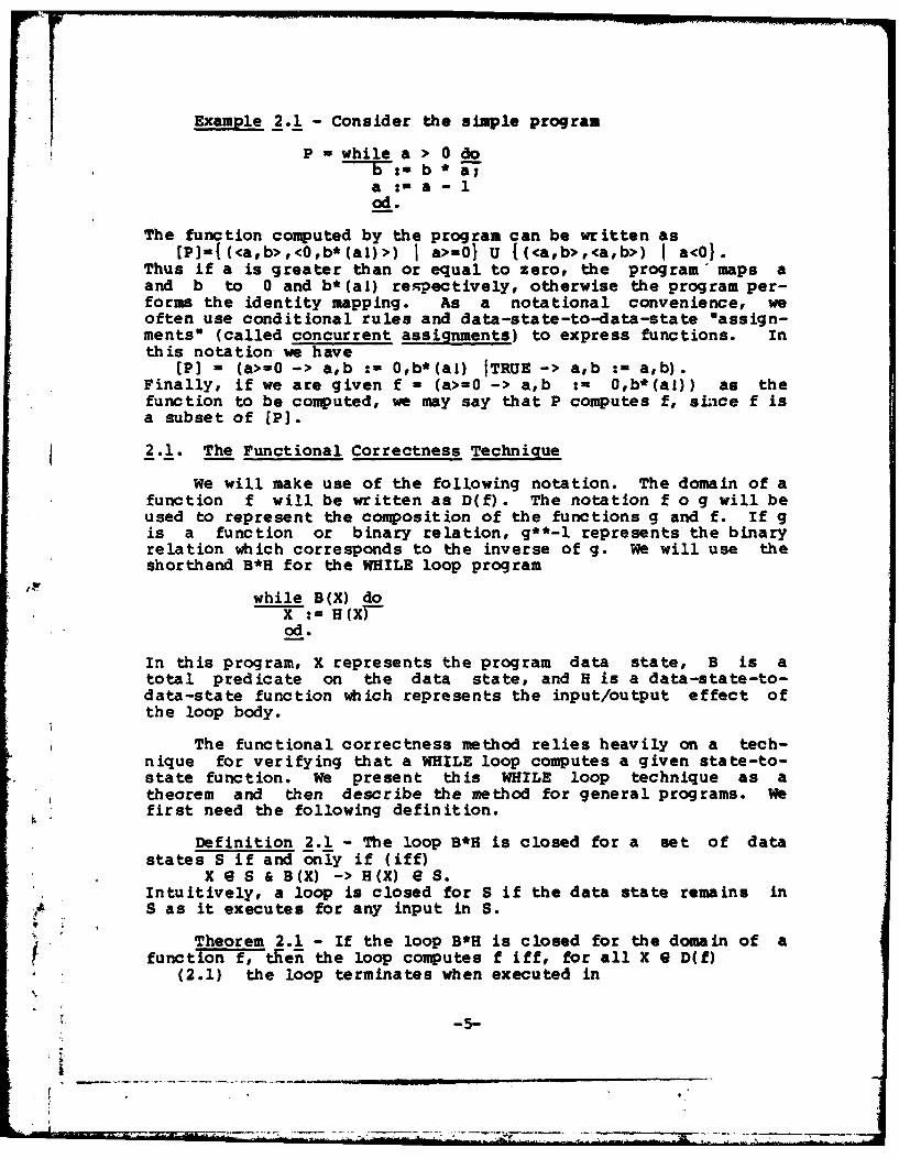
Example 2.1 - Consider the simple program

P - while a > 0 do5-:- b * a-a :- a-1od.

The function computed by the program can be written as[P]-I(<a,b>,<O,b*(a1)>) I a>-01 U {(<a,b>,<a,b>) I a<O1.

Thus if a is greater than or equal to zero, the program maps aand b to 0 and b*(al) respectively, otherwise the program per-forms the identity mapping. As a notational convenience, weoften use conditional rules and data-state-to-data-state "assign-ments" (called concurrent assignments) to express functions. Inthis notation we have

[P] - (a>=O -> a,b :- O,b*(a) ITRUE -> a,b := a,b).Finally, if we are given f - (a>-O -> a,b := O,b*(al)) as thefunction to be computed, we may say that P computes f, sice f isa subset of [P].

2.1. The Functional Correctness Technique

We will make use of the following notation. The domain of afunction f will be written as D(f). The notation f o g will beused to represent the composition of the functions g and f. If gis a function or binary relation, g**-l represents the binaryrelation which corresponds to the inverse of g. We will use theshorthand B*H for the WHILE loop program

while B(X) doX H (X)od.

In this program, X represents the program data state, B is atotal predicate on the data state, and H is a data-state-to-data-state function which represents the input/output effect ofthe loop body.

The functional correctness method relies heavily on a tech-nique for verifying that a WHILE loop computes a given state-to-state function. We present this WHILE loop technique as atheorem and then describe the method for general programs. Wefirst need the following definition.

Definition 2.1 - The loop B*H is closed for a set of datastates S if and only if (iff)

X e S & B(X) -> H(x) e s.Intuitively, a loop is closed for S if the data state remains inS as it executes for any input in S.

Theorem 2.1 - If the loop B*H is closed for the domain of afunction f, tKeii the loop computes f iff, for all X e D(f)

(2.1) the loop terminates when executed in

-5- ]

the initial state X,(2.2) B(X) - f(X) = f(H(X)), and(2.3) ~B(X) -> f(X) - X.

Proof - First, suppose (2.1), (2.2), and (2.3) hold. LetX[O] be any element of D(f). By condition (2.1) the loop mustproduce some output after a finite number of iterations. Let nrepresent this number of iterations, and let X[n] represent theoutput of the loop. Furthermore, let X[l], X[21, ... X[n-1] bethe intermediate states generated by the loop, i.e. for all isatisfying 0 <= i < n, we have B(X[i]) a X[i+l] - H(X[i]) andalso "B(X[n]). Condition (2.2) shows f(X[0]) - f(X[l]) -

f(Xn]). Condition (2.3) indicates f(X(n]) - X[n]. Thusf(X(OJ) - X(n] and the loop computes f.

Secondly, suppose the loop computes f. This fact would becontradicted if (2.1) were false. Suppose (2.2) were false, i.e.there exists an X e D(f) for which B(X) but f(X) f(H(X)). Fromthe closure requirement, H (X) e D(f) and the loop producesf(H(X)) when given the input H(X). But this implies the loop candistinguish between the. cases where H(X) is an input and the casewhere H(X) is an intermadiate result from the input X. However,this is impossible since the state describes the values of allprogram variables. Finally, if (2.3) were false, there wouldexist an X e D(f) for which the loop produces X as an output, butwhere f(X) X. Thus the loop must not compute f.

An important aspect of Theorem 2.1 is the absence of theneed for an inductive assertion or loop invariant. Under theconditions of the theorem, a loop can be proven or disprovendirectly from its function specification.

Example 2.2 - Using the loop P and function f of Example2.1, we shall show P computes f. D(f) is the set of all statessatisfying a >= 0. Since a is prevented from turning negative bythe loop predicate, the loop is closed for D(f) and Theorem 2.1can be applied. The termination condition (2.1) is valid since ais decremented in the loop body and has a lower bound of zero.Since H(<a,b>) - <a-l, b*a>, condition (2.2) is

a > 0 -> f(<a,b>) - f(<a-l,b*a>)which is

a > 0 -> <0,b*(al)> = <0,(b*a)*((a-1)1)>which can be shown to be valid using the associativity of * andthe definition a! a*((a-1)1). Condition (2.3) is

a - 0 -> <O,b*(al)> = <a,b>which is valid using the definition 01 - 1.

The functional correctness procedure is used to verify aprogram correct with respect to a function specification. Largeprograms must be broken down into subprograms whose intendedfunctions may be more easily derived or verified. These resultsare then used to show the program as a whole computes itsintended function. The exact procedure used to divide the

-6-

program into subprograms is not specified in the functionalcorrectness theory. In the interest of simplicity, the techniquepresented in this chapter is based on prime program decomposition[Linger, Mills & Witt 791. That is, correctness rules will beassociated with each prime program (or equivalently, with eachstatement type) in the source language. The reader should keepin mind, however, that in certain circumstances, other decomposi-tion strategies may lead to more efficient proofs. One such cir-cumstance is illustrated in Section 2.4.

In our presentation of the functional correctness procedure,we will consider simple Algol-like programs consisting of assign-ment, IF-THEN-ELSE, WHILE and compound statements. Before thecorrectness technique may be applied, the intended function ofeach loop in the program must be known. Furthermore, it isrequired that each loop be closed for the domain of its intendedfunction. These intended functions must either be supplied withthe program or some heuristic (see Chapters 4-5) must be employedby the verifier in order to derive a suitable intended functionfor each loop. This need for intended loop functions is analo-gous to the need for sufficiently strong loop invariants in aninductive assertion proof of correctness.

In order to prove that a structured statement S (i.e. aWHILE, IF-THEN-ELSE, or compound statement) computes a functionf, it is necessary to first derive the function(s) computed bythe component statement(s), and then to verify that S computes fusing the derived subfunctions. Consequently, the functionalcorrectness technique will be described by a set of functionderivation rules and a set of function verification rules. Theserules are given in Figure 2.1.

Before considering an example of the use of these rules, weintroduce two conventions that will simplify the proofs of largerprograms. First, we allow an assignment into only a portion ofthe data state in a concurrent assignment. In this case it isunderstood that the other data-state components are unmodified.

Example 2.3 - If a program has variables vl,v2,v3, thesequence of assignments

vl :- 4; v3 :- 7performs the program function

vl,v3 :a 4,7which is shorthand for

vl,v2,v3 :w 4,v2,7.

Secondly, if a function description is followed by a list ofof variables surrounded by # characters, then the function is

* intended to describe the program's effect on these variablesonly. Other variables are considered to have been set to anundefined or unspecified value.

-7-

'--Row-

Derive Rules -Used to compute [S.Dl: S = v: -e

1) Return [v:ine]D2: S - S1; S2

1) Derive [Si2) Deiv S213) Return [S2] o [Sli.

D3: S -if B ten SlelseS2 fiIT-eriveiTlI-2) Deri've [S213) Return (B->[S11 I TRUE->CS2]).

D4: S -while B do Slod1) Let f be the intended function

(either given or derived)2) Verify that while B do Si od

computesf3)Return f.

Verify Rules - Used to prove S computes f.

Vl: = :=e1) Derive [S]2) Show f(X)-Y -> [SJ(X) -Y.

V2: S -Sl;S21) Derive (S]2) Show f(X)-Y -> [SIMX Y.

V3: S -if Bthen SielseS2 fi=)Der iv S)1

2) Show f (X) -Y -> [S5I(X) *Y.

V4: S awhile B do Slod1) riveTSII2) Apply Theorem 2.1.

Figure 2.1 Derive and Verify Ruzles

Example 2.4 - if a program has variables vlv2,v3 that takeon values fromi dl,d2,d3, respectively, the function desncription

f - (vl > 0 -> v2,v3 :a vi+v3,v2) #v2,v3#is equivalent to

(vi > 0 -> vl,v2,v3 :- ?,vl+v3,v2).where ? represents an unspecified value. Note that in a sense,functions like f are not data-state-to-data-state functional moreI'accurately they are general relations. Eeg. in the example#<1,2,3> maps to <2,4,2> as well as <-2,4,2>. Howver, we adopt

*the view that fis adl xd2 xd3 to d2 xd3 mapping and in thislight, f is a function. we call {v2,v3) the range set for f,

written RS(f). Functions not using the # notation are assumed tohave the entire set of variables as their range set. Similarly,if the variables vrl,vr2,..,vrk are the necessary inputs to afunction description f, we say that {vrl,vr2...,vrkI is thedomain set for f, written DS(f). In Example 2.4, the domain setfor f T5 {vl,v2,v3} which happens to be the entire set of vari-ables, but this need not be the case. Note that some functions(i.e. constant functions) may have an empty domain set.

Example 2.5 - Consider the following program

Cl) -- (n>-O -> s :- SUM(i,l,m,i**n)) #s#1) a :- 1; s "= 01

C2) -- (n>-0 -> s:= s + SUM(i,a,m,i**n)) #s#2) while a <- m do3) "'-:= O; p -,1;

C3) -- (n>-j -> p,j:- p*a**(n-j),n)4) while j < n do5) " :- + I;6) p :-p*a7) od;8) s :s + p;9) a :-a+ 1

10) od.

In this example, the functions on the lines labeled Cl, C2 and C3are program comments and define the intended functions for theprogram, outer WHILE loop and inner WHILE loop respectively. The

Jp notation SUM(a,b,c,d) used in these functions stands for the sum-mation from a-b to c of the expression d. We use the notationFn-m as the derived function for lines n through m of the pro-gram.

Step 1) - Using derive rules D1 and D2 we getP5-6 - j,p :- j+l,p*a.

Step 2) - We must verify the inner loop computes its in-tended function. The closure condition and terminationcondition are easily verified. The other conditionsa re

j<n -> <p*a**(n-j),n> - <(p*a)*a**(n-(J+)),n>and

jmn -> <p*a**(n-j),n> - <p,J>which are true.

b Step 3) - Using Dl and D2 we derive F3-7 as follows:F3-7 - (n>-j -> pj - p*a**(n-j),n) o F3-3

- (n>-j -> p,j : p*a**(n-j),n) o j,p :- 0,1- (n>-O -> p,J : a**n,n).

Step 4) - Again with Dl and D2 we derive F3-9:73-9 - 78-9 o (n>-0 -> p,J :- a**nn)

a s,a :- s+p,a+l o (n>-0 -> p,J :- a**n,n)- (n>-O -> p,j,s,a :- a**n,n,s+a**n,a+l).

Step 5) - Now we are ready to show the outer loop computesits intended function. Again the closure and termina-tion conditions are easily shown. The remaining condi-

-9-

p ___

tions are (where n>=O)a<-m -> s+SU(i,a,m,i**n) - (s+a**n)+SUM(i,a+I,m,i**n)

anda>m -> s+SU(i,a,m,i**n) - a,

both of which are true.Step 6) -We now derive F1-10. Applying D2 we get

Fl-10 = (n>-0 -> s : s+SUM(i,a,m,i**n))#s# o fl-i= (n>-0 -> s : s+SUM(i,a,m,i**n))#s# o a,s :- 1,0= (n>-O -> s - SUM(i,l,m,i**n))#s#.

Step 7) - Since the intended program function agrees withFl-10, we conclude the program computes its intendedfu nct ion.

The functional correctness technique was developed by (Mills* 72, Mills 751. This verification method is compared and con-

trasted with the inductive assertion technique in (Basili &Noonan 80]. The presentation here is based on prime programdecomposition of composite programs and emphasizes the distinc-tion between function derivation and function verification in thecorrectness procedure.

The essential idea behind Theorem 2.1 can be traced to[McCarthy 62, McCarthy 63], in which a technique for ptoving twofunctions equivalent, "recursion induction," is described.Theorem 2.1 can be viewed as a specific application of this tech-nique. In (Manna & Pnueli 70, Manna 711 and more recently(Morris & Wegbreit 77], loop verification rules similar to thatstated in Theorem 2.1 are suggested. In (Basu & Misra 75], theauthors prove a result which corresponds to Theorem 2.1 for thecase where the loop contains local variables.

The closure requirement of Theorem 2.1 has received consid-erable attention. Several classes of loops which can be provedwithout the strict closure restriction are discussed in (Basu &Misra 76, Misra 78, Misra 79, Basu 80]. In (Wegbreit 77], how-ever, the author describes a class of programs for which theproblem of "generalizing" a loop specification in order tosatisfy the closure requirement is NP-complete.

2.2. The Loop Invariant f(XO0) - f(X)

An important implication of Theorem 2.1 is that a loop whichcomputes a function must maintain a particular property of thedata state across iterations. Specifically, after each itera-tion, the function value of the current data state must be thesame as the function value of the original input. In this sec-tion we discuss and expand on this characteristic of a loop whichis closed for the domain of a function it computes.

A loop assertion for the loop B*H is a boolean-valued* expression which yields the value TRUE just prior to each evalua-

tion of the predicate B. In general, a loop assertion A is afunction of the current values of the program variables (which we

-10-

will denote by X), as well as the values of the program variableson entry to the loop (denoted by XO). To emphasize these depen-dencies we write A(XO,X) to represent the loop assertion A.

Let D be a set of data states. A l invariant for B*Hover a set D is a boolean valued expres'son ATX0F,X)hich satis-fies the following conditions for all XO,X G D

(2.4) A(XO,XO)(2.5) A(XO,X) & B(X) -> A(XO,H(X)) & (H(X) e D).

Thus, if A(XO,X) is a loop invariant for B*R over D, then A(XOX)is a loop assertion under the assumption the loop begins execu-tion in a data state in D. Furthermore, the validity of thisfact can be demonstrated by an inductive argument based on thenumber of loop iterations.

Loop assertions are of interest because they can be used toestablish conditions which are valid when (and if) the executionof the loop terminates. Specifically, any assertion which can beinferred from

(2.6) A(XO,X) & "B(X)will be valid immediately following the loop.

It should be clear that for any loop B*H, there may be anarbitrary number of valid loop assertions. Indeed, the predicateTRUE is a trivial loop assertion for any WHILE loop. However,the stronger (more restrictive) the loop assertion, the more onecan conclude from condition (2.6). For a given state-to-statefunction f, we say that A(XO,X) is an f-adequate loop assertioniff A(XO,X) is a loop assertion and A(XO.X) icabiie in verl-fying that the loop computes the function f. More precisely, iff is a function, the condition for a loop assertion A(XO,X) beingan f-adequate loop assertion is

(2.7) XO G D(f) & A(XO,X) & -B(X) -> X-f(XO).A loop invariant A(XO,X) over some set containing D(f) for whichcondition (2.7) holds is an f-adequate loop invariant.

Example 2.6 - Let P denote the program

while a f {O,11 doi a > 0 thenI -- a -a ----2

i else a := a + 2 fi

Consider the following predicatesA1(<aO>,<a>) <-> TRUEA2(<aO>,<a>) <-> ADS(a) <- ABS(aO)A3(<aO>,<a>) <-> ODD(a) - ODD(aO)A4(<aO>,<a>) <-> ODD(a) - ODD(aO) & AS(s) <- AiS (a0)A5(<a0>,<a>) <-> ODD(a) a ODD(aO) OR (a=3 & aO2)

where AN8 denotes an absolute value function, and ODD returns 1if its argument is odd and 0 otherwise. Each of the 5 predicatesis a loop assertion. Let D be the set of all possible data

• -11-

states for P (i.e. D (<a> Ia is an integer)). Let f-(<a>,cODD(a)>) Ia is an integer), and consider A3. Since a G

10,11 implies a-ODD(a), we can infer a-ODD(aO) from A3(<a0>,ca>)&a 9 {0,11. Thus A3 is an f-adequate loop assertion. Simi-

larly, A4 and AS are f-adequate loop assertions, but neither Alnor A2 is restrictive enough to be f-adequate. Predicates A3 andA4 are loop invariants over D; however, since AS fails (2.5), itis not a loop invariant (a-3,aO-2 is a counter example).

Theorem 2.2 - If 3*H is closed for D(f) and B*H computes fthen f(XO) a f(X) is an f-adequate loop invariant over D(f), andfurthermore, it is the weakest such loop invariant in the sensethat if A(XO,X) is any f-adequate loop invariant over D(f) ,A (XO,X) -> f (X) -f (XO) for all XjXO G D(f) .

Proof - First we show that f(X)-f(XO) is a loop invariantover D(f). Condition (2.4) is f(XO)af(XO). From lTeorem 2.1,for all x e D(f),

B(XM -> f(X) - f (H(XM)Thus for all X,XO G D(f) ,

B(X) & f(XO)-f(X) -> f(XO)-f(X)-f(l(X)) -> f (XO) -f (fl(X))Adding the closure condition B(X) -> HMX e D(f) yields condition(2.5). Thus f (X) -f (XO) is a loop invariant over D(f) . Againfrom Th~eorem 2.1, for all X 6 D(f) ,

Thus for all XO Lz f(X)-Xf(X)-f(XO) & -B(X) -> f(X)-f(XO) &X f(X)-X -> f(XO)-X

wh ich shows f (X)-f (XO) is f -adequate.- Let A(XO,X) be a ny f-adequate loop invariant for 3*H over D(f), and let Z0,Z be ele-ments of D(f) such that A(ZO,Z). Since B*5 computes f and Z GD(f), there exists some sequence Z [1] ,Z 21, ... ,Z(ni (possiblywith n-l) where Z[l]nZ,, Z~nluf(Z)o -B(Zjnl), and with B(7Z(ij) &Z~i+l] - 5(Z~il) for all i satisfying 1 <- i < n. By condition(2.5) we have A(ZO,Z[l1), A(ZO,Z[21), ... ,A(ZO,Z[NJ),- thusA (Z 0, f(M and -B(f(Z)). Since ZO G D(f) and A(XO,X) is f-adequate,

A(ZO,f(Z)) & -B(f(Z)) -> M(O)-f()from condition (2.7). Thus for all ZO,Z 6 D(f),

A(ZO,Z) -> f(ZO)-f(Z).

Example 2.6 (continued) - In this example, A3 is of the formf(X)-f(XO). A3 is clearly weaker than the other f-adequate loopinvariant A4. it is worth noting that A3 is not weaker than AS,but AS is not a loop invariant, and A3 is not weaker than A2, but

.1 A2 is not f-adequate. This situation is illustrated in Figure2.2. The sets labeled Sl-SS are the sets of ordered pairs('<a0>,<a>' satisfying Al-AS, respectively, i.e.

SI. (ca0>,<a>) I AI(<aO>,ca')for 1-1,2,3,4 and 5. The diagram is partitioned in half with af 0,1) on the left and a e (0,11 on the right. Note that S4 (orthe set corresponding to any f-adequate loop invariant for thatmatter) is a subset of 83. Furthermore, the set corresponding toeach f-adequate loop assertion is identical where a 6 10,1).

-12-

This region of the diagram is precisely the set f.

Consider the problem of using Hoare's iteration axiom(2.8) I & B TX:H (X)I I -> I {B*H} I & -B

to prove the loop B*H computes a function f where B*H is closedfor D(f). In our terminology, if B*H is correct with respect tof, I must be a loop invariant over (at least) the set D(f) (oth-erwise X-f(XO) for all XO G D(f) cannot be inferred). However,using a loop invariant over a proper superset of D(f) is in gen-eral unnecessary, unless one is trying to show the loop computessome proper superset of f. If we choose to use a loop invariantI over exactly D(f), Theorem 2.2 tells us that f(X) -f(XO) is the

a 0 (0,11 a e {o,11

--- -- - - - - - - - -

S - Hfl1->IS~

S-3S-11$45,,

SSW

! 13

weakest invariant that will do the job. In a sense, the weakeran invariant is, the easier it is to verify that it is indeed aloop invariant (i.e. that the antecedent to (2.8) is true),because it says less (is less restrictive, is satisfied by moredata states, etc.) than other loop invariants. Along theselines, one might conclude that if a loop is closed for the domainof a function f, Theorem 2.2 gives a formula for the weasiest"loop invariant over D(f) that can be used to verify the loop com-putes f.

Let us again consider loop invariants and functions as setsof ordered pairs of data states. Let B*H compute f and letA(XO,X) be an f-adequate loop invariant. It is clear that inthis case t(XO,X) I A (XO,X) & -B(X) & (XO G D(f)))is precisely f. That is, f must be the portion of the setrepresented by A(X0,X) obtained by restricting the domain to D(f)and discarding members whose second component cause B to evaluateto TRUE. Can the set represented by A(XO,X) be determined fromf? No, since in general, there are many f-adequate invariantsover D(f) and the validity of some will depend on the details ofB and H (e.g. A4 in Example 2.6). However, Theorem 2.2 gives usa technique for constructing the only f-adequate invariant overD(f) that will be valid for an B and H, provided B*H computes fand is closed for D(f). Spefically, this invariant couples anelement of D(f) with any other element of D(f) which belongs tothe same level set of f. (S is a level set of f iff there existsa Y such that S-{Xff(X)-YI). Put another way - all f-adequateloop invariants over D(f) describe what the loop does (i.e. theycan be used to show the loop computes f), and some may also con-tain information about how the final result is achieved. Thatis, one might be able to use an f-adequate loop invariant to makea statement about the intermediate states generated by the loopon some inputs. The intermediate states "predicted" by the weak-est invariant f(X)-f(XO) is the set of all intermediate statesthat could possibly be generated by any loop B*H that computesthe function. Thus, the invariant f(X)-f(XO) can be thought ofas occupying a unique position in the spectrum of all possibleloop invariants: it is strong enough to describe the net effectof the loop on the input set D(f) and yet is sufficiently weakthat it offers no hint about the method used to achieve theeffec t.

Example 2.7 - Consider the following program

while a > 0 doa m-a- : "7,c :- c +~ bod.

IThis loop computes the functionf a (a>-0 -> a,b,c :- 0,bc+a*b).

From Theorem 2.2, we know that

-14-

A(<aO,bO,c>,<a,b,c>) ,-> <ObO ,cO+aO*bO>,<O,b,c+atb>is the weakest f-adequate invariant over a>-01.Consider the saale input <4,10,7>. Our loop will produce theseries of states <4,10,7>, <3,10,17>, <2,10,27>, <1,10,37>,

; <0,10,47>. of course, our invariant agrees with these intermedi-ate states (i.e. A(<4,10,7>,<4,10,7>), A(<4,10,7>,<3,10,17>),.., A(<4,10,7>,<0,10,47>)), but it also agrees with <6,10,-13>. Weconclude then, that it is possible for some loop which computes fto produce an intermediate state <6,10,-13> while mapping<4,10,7> to <0,10,47>. Furthermore, no loop which computes fcould produce <6,10,-12> as an intermediate state from the input<4,10,7> since the invariant would be violated.

To emphasize this point, we define an f-adequate invariantA(XO,X) over D(f) for B*H to be an internal invariant if A(XO,X)implies that B*H will generate X as an intermediate state whenmapping X0 to f(XO). Intuitively, an internal invariant captureswhat the loop does as well as a great deal of how the loop works.In our example, babO & c-c0+b*(a0-a) & 0<-a<-aO is an internalinvariant, but A(<aO,bO,cO>,<a,b,c>) as defined above is not (thestate <6,10,-13> on input <4,10,7> is a counter example). It canbe proven that if f is any nonempty function other than the iden-tity function, no loop for computing f exists for whichf(X)=f(XO) is an internal invariant[l]. However, if we considernondeterministic loops and weaken the definition of an internalinvariant to one where A(XO,X) implies X may be generated by B*Hwhen mapping XO to f(XO), such a loop can always be found. Thisloop would nondeterministically switch states so as to remain inthe same level set of f. Our example program could be modifiedin such a manner as follows:

while a > 0 dot:w "some integer value greater than or equal

to zero";c . c + b * (a-t);a :tod

and corresponds to a "blind search" implementation of the func-tion.

In [Basu & Misra 751, the authors emphasize the differencebetween loop invariants and loop assertions. The fact that f(X)

El] Outline of proof: Let f(Y)#Y, B*H compute f and suppoethe f-adequate invariant f(X)-f(XO) over D(f) for B*lH is aninternal invariant. ft must have B(Y). By (2.2) f(Y)-E(H(Y)).Consider H(Y) as a fresh input. Since f(X)-f(XO) is an internalinvariant and f(Y)-f(H(Y)), the loop must eventually produce in-termediate state Y, which must then produce H(Y). Thus B*H failsto terminate and does not compute f.

-15-

, _ 1 . .. . _ . . I. ... . . .. . . . .. -_ = _ . ' J - i ' I " " - T, _ : ' . . .

- f(XO) is an f-adequate loop invariant appears in [Basu & i4sra75, Linger, Kills a Witt 791. The independence of this loopinvariant from the characteristics of the loop body is discussedin [Basu a Kisra 751.

2.3. Comparing the Hoare and Mills L Proof Rules

An alternative to using Theorem 2.1 in showing a loop com-putes a function is to apply Hoare's inductive assertion verifi-cation technique. That is, one could verify P {B*l 0 where

P <-> X-XO a X e D(f), andQ <-> X-f(XO)

by demonstrating the following for some predicate I:Al: P->IA2: B a I IX: -(X)) IA3: B &I-> .

* Strictly speaking, conditions Al through 13 show partial correct-ness; to show total correctness, one must also prove

A4: B*1 terminates for any input state satisfying P.

We now wish to compare these verification conditions withthe functional verification conditions. Recalling from Theorem2.1, if B* is closed for D(f), the functional verification rulesare:

Fl: X G D(f) -> B*N terminates for the input XF2: X D( f) G B(X) -> f(X) - f(N(X))F3: X 6 D(f) 6 "B(X) -> f(X) - X.

In the following discussion we adopt the convention that if f isa function and X is not in D(f), then f(X)-Z is false for anyformula Z.

Theorem 2.3 - Let B*H be closed for D(f). If f(X)-f(XO) isused as the predicate I in Al-A3, then Al & A2 & A3 & A4 <-> F1 &F2 & F3. That is, the functional verification conditions Fl-F3are equivalent to the special case of the inductive assertionverification conditions A1-A4 which results from using f(X)-f(XO)as the predicate I. In particular, if I <-> f(X)-f(Xo) in theinductive assertion rules, then

Al <-> TRUE,A2 <-> F2 provided X 0 D(f) & B(X) -> X S D(H),A3 <-> F3,A4 <-> Fl.

Proof - We begin by noting that the termination conditionsA4 and F1 are identical, thus A4 <-> Fl. Secondly Al is

X-XO & X 0 D(f) -> f(X)-f(XO)which is clearly true for any f. Combining with our first resultyields Al a A4 <-> P1. Condition A3 can be rewritten as

"3(X) & f(X)-f(XO) -> Xf(XO)which is trivially true for any XXO outside D(f). Thus A3 mybe rewritten as

-111.3*t: XXO D( f) & -B (X) & f (),-f.(XO) -> Xnf (XO).

moeta Y7 ycniern4h a hr sO

i

Furthermore, F3 -> AV by considering the case where XO G D(f)and f(X)-f(XO). Now we have A3 <-> A3V <-> F3 and adding this toour result above we get Al & A3 & A4 <-> Fl & F3. We next proveA2 & A4 <-> F1 & F2. This combined with the above equivalenceyields the desired result Al & A2 & A3 & A4 <-> 7l & F2 & F3.Note that if there exists an X B D(f) such that B(X) but H(X) isnot defined, then the loop itself will be undefined for X, bothA4 and F1 will be false and A2 & A4 <-> F2 & Fl. We now considerthe other case where for all X e D(f), B(X) -> X e D(H). In thissituation we will show A2 <-> F2; combining with A4 <-> F1 yieldsA2 & A4 <-> F2 & Fl. Rule A2 may be rewritten as

3(X) & f(X)=f(XO) {X:uH(X)} f(X),f(XO)which again is trivially true if X or XO is outside D(f) ; thus A2is equivalent to

X, XO B D(f) & B(X) & f(X)=f(XO) {X:uH(X)} f(X)-f(Xo).Since H is defined for any input x e D(f) such that B(X) byhypothesis, this may be transformed using Hoare's axiom ofassignment to the implication

A2V: X,XO 6 D(f) & B(X) & f(X)=f(XO) -> f(H(X)) -f(XO).As before, we can show A2*->F2 by considering the case whereX=XO, and F2->A2 * by considering the case where XO G D(f) andf(X)=f(XO). Thus A2 <-> A2* <-> F2 which implies A2 <-> F2.This completes the proof of the theorem.

The purpose of Theorem 2.3 is to allow us to view the func-tional verification conditions as verification conditions in aninductive assertion proof. Not surprisingly, both techniqueshave identical termination requirements. If the termination con-dition is met, F2 amounts to a proof that f(X)-f(Xo) is a loopinvariant predicate. Condition F3 amounts to an application ofthe "Rule of Consequence," testing that the desired result can beimplied from the predicate f(X)=f(XO) and the negation of thepredicate B.

2.4. Subgoal Induction and Functional Correctness

Subgoal induction is a verification technique due to [Morris& Wegbreit 77]. It is based largely on work appearing in [Manna &Pnueli 70, Manna 711. In this section we compare subgoal induc-tion to the functional correctness approach described above.

We first note that subgoal induction can be viewed as a gen-eralization of the functional approach presented here in thatsubgoal induction can be used to prove a program correct withrespect to a general input-output relation. A consequence ofthis generality, however, is that the subgoal induction verifica-tion conditions are sufficient but not necessary for correctness;

*that is, in general, no conclusion can be drawn if the subgoalinduction verification conditions are invalid. Provided the clo-sure requirement is satisfied, the functional verification conOi-tions (as well as the subgoal induction verification conditionswhen applied to the same problem) are sufficient and necessaryconditions for correctness. Results in [Misra 771 suggest that

-17-

it is not possible to obtain necessary verification conditionsfor general input-output relations without considering thedetails of the loop body.

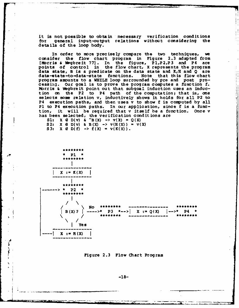
In order to more precisely compare the two techniques, weconsider the flow chart program in Figure 2.3 adapted from[Morris & Wegbreit 77]. In the figure, Pl,P2,P3 and P4 arepoints of control in the flow chart, X represents the programdata state, B is a predicate on the data state and K,H and Q aredata-state-to-data-state functions. Note that this flow chartprogram amounts to a WHILE loop surrounded by pre and post pro-cessing. Our goal is to prove the program computes a function f.Morris & Wegbreit point out that subgoal induction uses an induc-tion on the P2 to P4 path of the computation; that is, oneselects some relation v, inductively shows it holds for all P2 toP4 execution paths, and then uses v to show f is computed by allP1 to P4 execution paths. In our application, since f is a func-tion, it will be required that v itself be a function. Once vhas been selected, the verification conditions are

Sl: x e D(v) & -B(X) -> v(X) = Q(X)S2: x e D(v) & B(X) -> v(H(X)) = v(X)S3: X e D(f) -> f(X) = v(K(X)).

*P1*

X X:-K(X) I* ** **** *

, * P2 *

/***o*******

B B(X) ? I-->* P3 *-->I X :- Q)(X) 1-->* P4*

IYes--- I X---X) I

Figure 2.3 Flow Chart Program

****-18-

Note that Sl and S2 test the validity of v; S3 checks that v canbe used to show the program computes f.

The functional verification theory presented here is similarwith the exception that the function Q is not included in theinduction path. We select some function g and show it holds forall P2 to P3 execution paths (i.e. we show the WHILE loop com-putes g) and then use g to show f is computed by all P1 to P4execution paths. Once g has been selected, the verification con-ditions are

Fl: x e D(g) & ~B(X) -> g(X)-XF2: X e D(g) & B(X) -> g(H(X)) = g(X)F3: X e D(f) -> f(X) = Q(g(K(X))).

Note that both techniques require the invention of an inter-mediate hypothesis which must be verified in a "subproof." Thishypothesis is then used to show the program computes f. Thefunction Q in the flow chart program is absorbed into the inter-mediate hypothesis in the subgoal induction case; it is separatefrom the intermediate hypothesis in the functional case. Indeed,the two intermediate hypotheses are related by

v o g.

If Q is a null operation (identity function), the intermedi-ate hypotheses and verification conditions of the two techniquesare identical. A significant difference between the two tech-niques, however, can be seen by examining the case where K is anull operation. If the loop is closed for D(f), subgoal induc-,V

tion enjoys an advantage since f can be used as the intermediatehypothesis. That is, the subgoal induction verification condi-tions are simply

SI': x e D(f) & B(X) -Q 0(X) = f(X)82': X e D(f) & B(X) -> f(H(X)) f(X).

In the functional case, one must still derive an hypothesisfor - the loop function g. A heuristic which can be applied hereis to restrict one's attention to functions which are subsets ofQ**-l o f. However, it is worth emphasizing that this rule neednot completely specify g since, in general, Q**-l o f is not afunction. Once g has been selected, the verification conditionsare

Fl'*: x e D(g) & -B(x) ->g(x)-x

F2': x e D(g) & B(X) - g(H(X))-g(X)F3Y: X e D(f) -> f(X) i (g(X)).

The difference between the two techniques in this case isdue to the prime program decomposition nature of the functionalcorrectness algorithm described in Section 2.1. A more efficientproof is realized by treating the loop and the function 0 as a

* whole. Accordingly, correctness rules for this program formmight be incorporated into the prime program functional correct-

, ness method described earlier. The validity of these rules canbe demonstrated in a manner quite similar to the proof of Theorem

-19-

2.1.

Example 2.8 - We wish to show the program

while x g 10,1,2,3} doif x < 0 then x : x + 4

el-se x : x - 4 fiod;

if x > 1 then x :- x - 2 fi

computes the function f={(<x>,<ODD(x)>)j. The Subgoal inductionverification conditions are

x e {0,1,2,31 -> Q(x) - ODD(x), andx 0 10,1,2,3 -> ODD(H(x)) = ODD(x), where

Q(x) = if x > 1 then x-2 else x, andH(x) - if x < 0 then x+4 else x-4.

Both these conditions are straightforward. Now let us considerthe prime program functional case. Suppose we are given (or mayderive) the intended loop function

g = (<xO>,cx>) I x e 10,1,2,31 & x md 4 = xO mod 4}.We can verify that the loop computes g by demonstrating Fl* andF2'. Condition F3 uses g to complete the proof.

The difficulty with splitting up the program in this exampleis that it requires the verifier to "dig out" unnecessary detailsconcerning the effect of the loop. One need not determine expli-citly the function computed by the loop in order to prove theprogram correct. The only important loop effect (as far as thecorrectness of the program is concerned) is x e 10,1,2,31 andODD(x) = ODD(xO). In this example, treating the program as awhole appears superior since it only tests for the essentialcharacteristics of the program components.

It is worth observing that, provided the loop is closed forD(f), an inductive assertion proof of a program of this formcould be accomplished by using the loop invariant f(X) - f(XO).The verification conditions in this case would be equivalent tothe subgoal induction verification conditions. Note that, ingeneral (as in our example), f(X) - f(X0) is too weak an invari-ant to be g-adequate for the intended loop function g above.

2.5. Initialized Loops

The preceding section indicates that it is occasionallyadvantageous to consider a program as a whole rather than to con-sider its prime programs individually. In this section we

A attempt to apply the same philosophy to the initialized loop pro-gram form and use the result as a basis from which to compare thefunctional and inductive assertion approaches to this particularverification problem.

-20-

We will again consider the program in Figure 2.3 with theunderstanding that Q is a null operation (identity function). Wewant to prove that the program computes a function f, i.e. that fholds for all P1 to P3 paths. We have seen that prime programfunctional correctness involves an induction on the P2 to P3 exe-cution path using an intermediate hypothesis g. An inductiveassertion proof would involve an induction on the P1 to P2 execu-tion path using some limited loop invariant A(XOX) [Linger,Mills & Witt 79]. A limited loop invariant differs from thosediscussed previously in that it takes into account the initiali-zation preceding the loop. One of the objectives of this sectionis to discuss the relative difficulties of synthesizing theintermediate hypotheses g and A.

We now reason about whether there might be an efficient wayto verify the program by treating it as a uhole (i.e. rather thantreating the initialization and the loop individually). In orderfor the program to compute f, it must be that K(X)-K(Y) ->f(X)=f(Y). Consequently, the relation represented by f o (K**-l)is a function and is a candidate for the intermediate hypothesisg. Indeed, the initialized loop program is correct with respectto f iff g - f o (K**-l) is a function and the WHILE loop (byitself) is correct wrt g. Unfortunately, the domain of thisfunction is the image of D(f) through K, and since the purpose ofthe initialization is often to provide a specific "startingpoint" for the loop, the loop will seldom be closed for thedomain of this function. Thus the problem of finding anappropriate g can be thought of as one of generalizing f o (K**-1).

Example 2.9 - We want to show the program

s :- 0; i :- 0;while i < n do

i :=i +1s := s + a[i)od

computesf - s:-SUM(k,l,n,a[k])#s#.

As before, SUM(k,l,n,a(k]) is a notation for a[l)+a[21++a(n]. If K represents the function performed by the initializa-tion, f o (K**-l) is

(s-0,i-O -> s:=SUM(k,l,n,a[k]))#s#.Note that the loop is not closed for the domain of this function.To verify the program using the functional method, this functionmust be generalized to a function such as

Sg = s:-s+SUM(ki+ln,alkI)#s#.

We now consider the relative difficulties of synthesizing a*suitable loop function g (for a functional proof) and synthesiz-

ing an adequate limited loop invariant (for an inductive asser-tion proof). If we have a satisfactory g for a functional proof

-21-

of the program, the analysis in Section 2.2 indicates that theinvariant A(XO,X) <-> g(X)-g(XO) over D(g) can be used to showthe loop computes g; absorbing the initialization X:wK(X) intothe invariant gives the result that the limited invariant A(XO,X)<-> g(X)-g(K(XO)) can be used to prove the initialized loop pro-gram computes g o K - f. We now try to go the other way. Sup-pose we have an appropriate limited loop invariant A(XO,X) for aninductive assertion proof of the program, can we derive from thatan adequate loop function g? We motivate the result as follows:we could obtain an equivalent program by modifying the initiali-zation to (nondeterministically) map XO to X if A(XO,X) is true.The modified program (assuming termination) must still computethe same function; if the initialization maps XO to anythingother than K(XO), the effect will simply be to alter the numberof iterations executed by the loop. By the same argument thatwas used to show that the loop, assuming correctness, must com-pute f o (K**-l), the loop must also compute f o (A(XO,X)**-l).That is, if A(XO,X) holds for some XO e D(f) and for some X, theloop mu st map X to f(XO). Note that the loop is necessarilyclosed for the domain of this function; otherwise the invariantwould be violated. The proper conclusion is that the synthesisof an adequate loop function and the synthesis of a suitableinvariant are equivalent problems in the sense that a solution toone problem implies a solution to the other problem.

Example 2.9 (continued) - An inductive assertion proof ofour program might use the limited invariant s-SUM(k,l,i,a[k]) &0<-i<-n. Note that this invariant implies the invariantg(K(XO))=g(X) discussed above (where g and K are as defined pre-viously). Using the technique outlined above, we may derive fromthis invariant the loop functiong' = (s=SUM(k,l,i,a(k]), 0<-i<-n -> s:-SUM(kl,n,a[k]))#s#.

Observe that this is quite different from the original g, butthat g' is quite satisfactory for a functional proof of correct-ness. It may seem puzzling that g*(XO)=g*(X) is the constantinvariant TRUE over the set D(g*) and yet Theorem 2.2 states thatsuch an invariant must be gA-adequate. This is not a contradic-tion, however, since

TRUE, i>-n -> s=SUM(k,l,n,a[k])is valid for any state in D(g). Similarly, a functional proofthat the loop computes g" is trivial with the exception of veri-fying that the closure requirement is satisfied. This is nocoincidence: proving closure is equivalent to demonstrating thevalidity of the loop invariant.

The translation between loop invariants and intermediatehypotheses in a subgoal induction proof is discussed in [Morris &Wegbreit 77, King 80]. In Chapter 3, we propose a new verifica-tion strategy for initialized loop programs which is based on theabove mentioned notion of a nondeterministic loop initialization.

-22-

* 2.6. Discussion

Our purpose in this chapter has been to explain the func-tional verification technique in light of other program correct-ness theories. The functional technique is based on Theorem 2.1which provides a method for proving/disproving a loop correctwith respect to a functional specification when the loop isclosed for the domain of the function.

In Theorem 2.2, a loop invariant derived from a functionalspecification is shown to be the weakest invariant over thedomain of the function which can be used to test the correctnessof the loop. Theorem 2.3 indicates that the functional correct-ness technique for loops is actually the special case of theinductive assertion method that results from using this particu-lar loop invariant as an inductive assertion. The significanceof this observation is that the functional correctness techniquefor loops can be viewed either as an alternative verificationprocedure to the inductive assertion method or as a heuristic forderiving loop invariants.

The subgoal induction technique seems quite similar to thefunctional method; the two techniques often produce identicalverification conditions. We have, however, observed an examplewhere the subgoal induction method appears superior to functionalcorrectness based on prime program decomposition. In the follow-ing chapter, the idea of a proof transformation is introduced andis proposed as a decomposition strategy which overcomes thisdeficiency in prime program decomposition.

We have examined the inductive assertion and functionalmethods for dealing with initialized loops. We have shown thatthe problems of finding a suitable loop invariant and finding anadequate loop function are essentially identical. The resultindicates that for this class of programs, the two methods aretheoretically equivalent; that is, there is no theoretical jus-tification for selecting one method over the other.

In Chapter 4, we deal with the functional correctnessrequirement that each program loop be documented with anappropriate intended function. In order to alleviate this prob-lem, a heuristic technique is proposed which can be used as anaid in ascertaining undocumented intended functions for programloops.

We explained in Section 2.5 that it is possible to obtain aloop function for a loop preceded by initialization based on theinitialization and the program specification. This function,

.A however, usually has a restricted domain and must then be gen-eralized to meet the closure requirement of Theorem 2.1. InChapter 5, we discuss a class of loops for which these generali-zations may be obtained in a systematic manner.

-23-

3. A New Verification Strategy For Iterative Programs

The difficulties associated with the general verification ofcomputer programs are well known. Chief among these difficultiesis the problem of creating a suitable inductive hypothesis forprograms which use iteration or recursion. A large number ofguidelines or heuristics for the construction of these hypotheseshave appeared in the literature. Particularly promising areresults along the lines of Theorem 2.1 [Mills 75, Basu & Misra75, Wegbreit 77, Morris & Wegbreit 771 which show that for a par-ticular class of program/specification pairs, an appropriateinductive hypothesis may be obtained directly from the specifica-tion. The direct consequence of these results is that for averification problem in this class, the program can beproven/disproven correct with respect to its specification(assuming termination) by testing several verification conditionsbased on the specification and characteristics of the programcomponents. Unfortunately, this class is rather restricted and,as a result, many verification problems which arise naturally inpractice are not covered by these results.

In this chapter, a verification strategy is described whichis based an the idea of applying a correctness/incorrectnesspreserving transformation to the program under consideration.The motivation behind the transformation is to produce a verifi-cation problem such that, in a manner similar to that in theabove mentioned work, an inductive hypothesis can be directlyobtained. Thus we are proposing replacing the problem of syn-thesizing an inductive hypothesis with one of discovering an ade-quate correctness/incorrectness preserving transformation. In anumber of examples we have studied, the latter problem appears tobe more tractable.

In the remainder of this section we discuss a general verif-ication problem which occurs often in practice and then suggestthe idea of a transformation as a means to solve the problem. Anumber of heuristics for discovering an appropriate transforma-tion are given in Section 3.1 and are illustrated with examples.In Section 3.2, the proposed solution is compared and contrastedwith the inductive assertion and subgoal induction approaches tothe verification problem. Finally, the application of the tech-nique to more complex program forms is discussed in Section 3.3.

In our analysis, we will consider a program P of the form

X : K(X)while B(X) do

X :- H (XF* .~*od;

X :a Q(X)

where X is the program data state, K, H and Q represent data-state-to-data-state functions and B is a predicate on the data

-24-

state. For the present we assume each of the functions and thepredicate is explicitly known; this requirement regarding thefunction Q is relaxed in Section 3.3. We assume that the programspecification is formulated as a function mapping the input datastate to the portion of the output data state which correspondsto the program variables whose final values are of interest. Wewill use a function e which extracts from any data state the datastate portion corresponding to these variables. Thus for thisverification problem, P is correct with respect to its specifica-tion function f if and only if for any X in D(f), [P) (X) isdefined and f(X)-e([P](X)).

Let TAIL be the portion of P which follows the initializa-tion X :- K(X), i.e. TAIL is the WHILE loop followed by theassignment X :- Q(X). We begin with the following:

Observation 1 - P is correct wrt f iff TAIL is correct wrtthe input/output relation

g = {(X,Y) I + XO G D(f) )- (K(XO)-X & f(XO)-Y)}.

That is, P is correct wrt f iff on data states X which areoutput by K on input XO L D(f), TAIL produces f(XO). For themoment, we make the following two assumptions:

FUNCTION: The relation g is a function, i.e.K(XO)-K(Xl) -> f(XO)-f(Xl)

for all XO, Xl e D(f), andCOSURE: The WHILE loop is closed (see Section 2.1) for

the domain of g, i.e.,A K(XO)-X, B(X) -> 4 Xl e D(f) )- K(Xl)-H(X)

for all XO G D(f) [21.

Given these two assumptions, it is easy to state the neces-sary and sufficient verification conditions for the correctnessof TAIL (assuming termination) wrt g. These are (adapted from[Mills 75, Basu & Misra 75, Morris & Wegbreit 77])

X e D(g), B(X) -> g(X)-g(H(X))X e D(g), ~B(X) -> g(X)-e(Q(X))

and are called the iteration and boundary conditions, respec-tively, in [Misra 78]. They are equivalent to

XO G D(f), K(XO)-X, B(X) -> g(X)-g(H(X))XO L D(f), K(XO)-X, ~B(X) -> g(X)-e(Q(X))

i.e.XO G D(f), B(K(XO)) -> g(K(X0))-g(H(K(X0)))Xo e D(f), -B(K(XO)) -> g(K(XO))-e(Q(K(XO)))

i.e.

S[2] Throughout this dissertation, we frequently use the nota-Pl, P2, ... , PN -> B

for the slightly longerf P1 P2 &.. PN -> B.

-25-

I. z

XOPX. e D(f), B(K(XO)), K(Xl)-H(K(XO)) -'g(K(XO))-g(K(X1))

XO e D(f) -B(K(XO)) -'g(K(XO))-e(Q(1K(XO)))

i.e.I TERATION:

XO,X1 e D(f), B(K(XO)), K(Xl)=H(K(XO)) ->f(XO)nf(Xl)

BOUNDARY:XO 0 D(f) -B(K(XO)) ->f(XO)me(Q(K(XO))).

We conclude as follows:

Observation 2 - Suppose FUNCTION and CLOSURE hold. P iscorrect wrt f (assuming termination) iff ITERATION and BOUNDARYh old.

Example 3.1 - Consider the following program

I a>-o}a :- a/2;while a 0 10,11 do

a :- a - 2od;

a := (if a-0 then 1 else 0)I a-EVEN (aO/2) T-

In this program, the data state consists of the single integervariable a and will be represented by <a>. The function EVEN(a)appearing in the program postcondition returns 1 if its argumentis even and 0 otherwise. The specification function f for thisprogram is

f(<aO)-a <-> aO>-0 & a-EVEN(aO/2)which implies

<aO> e D(f) <-> a0>0O.This program relates to the general program form above as follows

K(caO>)-<a> <-> a-aO/2B(<a>) <-> a '% {0,11H(<aO>)=<a> <-> awaO-2Q(<aO>)=<a> <-> (aO=0 & a-1) OR (aO#0 G a-0)e( <a> )-a.

Note that assumptions FUNCTION and CLOSURE hold. if the programterminates for all inputs in D(f) , it is correct wrt its specifi-cation iff conditions ITERATION and BOUNDARY hold. These can bewrittenaO>-0, al'-0, aO/2 it 10,11, al/2-aO/2 - 2

- > EVEN (aO/ 2) -EVEN (al/ 2)and

aO>-0, aO/2 e 10,11 -> EVEN(aO/2)-(if aO/2-0 the 1 else 0)respectively.

w At this point we stop to consider the assuiptions we havemade. Suppose assumption FUNCTION is false, but CLOSURE holds.f Thus we have XO, Xl e D(f) satisfying

K(XO)inK(Xl) G f(XO)pf(Xl).Now if B(K(X)), then K(X2)-H(K(XO)) for some X2 63 D(f) by CL0-SURE. If ITERATION was valid, we would have f(XO)-f(X2) as well

* -26-

as f(Xl)-f(X2). Since this contradicts our hypothesis, ITEATIONdoes not hold. On the other hand, suppose "B(K(XO)). If BOUN-DARY held, we would have f(XO)-e(Q(K(XO))) as well asf(Xl)-e(Q(K(Xl))). The contradiction leads us to conclude thatif UNCTION is false, but CLOSURE holds, (at least) one of ITZRA-TION and BOUNDARY is false. Since FUNCTION being false implies Pis not correct wrt f (i.e. [P](XO)-(P](Xl), but f(XO)#f(Xl)),this leads us to the following:

Observation 3 - Suppose CLOSURE holds. P is correct wrt f(assuming termination) iff ITEATION and BOUNDARY hold.

Unfortunately, it is much more difficult to deal with thereliance on assumption CLOSURE. We can, however, gain insightinto the problem by studying CLOSURE and its relation to condi-tion ITEATION. Imagine P executing on some input in D(f) andconsider the sequence of intermediate data states on which thepredicate B is evaluated. CLOSURE requires that each of theseintermediate states be "reachable" through the function K forsome input element of D(f). It is this reachability that enablescondition ITERATION to test whether this sequence of states stayson the right "track," or more specifically, that the inverseimages of these states through K remain in the same level set off.

Most often in practice, however, the purpose of the initial-ization K is to "constrain" the data state, thereby providingsome specific "starting point" for the loop execution. In thiscase, the intermediate data states will not be reachable throughK and, as a result, condition ITERATION may well hold for thesimple reason that it is vacuously true, i.e. the termK(Xl)-H(K(XO)) will be false for all Xl. Rather than abandoningthis approach to the verification of P, however, the solutionsuggested here is to "correct" the problem and proceed.

Consider substituting for K a suitable replacement initiali-zation K'. By "suitable" here, we mean that the output of K"must be sufficiently unconstrained so that CLOSURE holds for Ko,and furthermore, that the substitution preserves the terminationand correctness/incorrectness properties of the program P. Thefollowing definition formalizes this idea.

Definition 3.1 - Let P be the program P with the initiali-zation K replaced by K'. K is a reduction hypothesis iff C)-SURE holds for K and each of

TERMINATES: For inputs in D(f), P terminates -> P" terminates,and

4 PRESERVES: P is correct Wrt f iff P is correct wrt fis satisfied.

The significance of the definition is that once a reductionhypothesis K has been located, we can prove/disprove thecorrectness of the original program by proving its termination

-27-

and verifying ITERATION and BOUNDARY with K substituted for K.

The proposed solution of finding a reduction hypothesis isanalogous to finding an adequate loop invariant for an inductiveassertion proof [Hoare 691, or finding an appropriate loop func-tion for a functional [Mills 751 or subgoal induction [Morris &Wegbreit 77] proof. We justify proposing an alternative to thesestandard techniques for the following r-asons:

a) a reduction hypothesis has a uni4. intuition behindit; in a number of cases, this leads rather natu-rally to a solution,

b) the class of reduction hypotheses bears an interestingrelationship to the class of adequate loop invariantsfor P,

c) unlike the technique of inductive assertions, it ispossible to disprove an incorrect program withoutconsidering the program beyond the loop, i.e. by dis-p rov ing ITEATION,

d) in the case there is no initialization (i.e. K is theidentity function) and the loop is closed for D(f)(or, more generally, any time CWSURE holds for K), avery efficient proof results since K itself is a re-duction hypothesis, and

e) the reduction hypothesis solution provides continuitybetween the cases where CLOSURE does and does nothold; an understanding of "whym CLOSURE does nothold, for example, can provide insight into how tocreate K from K.

3.1. Constructing a Reduction Hypothesis

In this section we will consider several heuristics forcreating a reduction hypothesis for P and will illustrate theiruse on example programs. We begin with some preliminary remarks.

In the discussion in the preceding section, we assumed thatthe program pieces corresponding to K, H and Q were determinis-tic, that is, we assumed their semantics (i.e. their input/outputEeWav ior) could be represented by data-state-to-data-state func-tions. The above results, however, extend in the natural way tothe case where subprograms in P are nondeterministic provided oneswitches to a slightly more awkward relational notation forrepresenting these subprograms. In particular, we will beinterested in the case where the initialization is nondeterminis-tic since it turns out that this kind of initialization is oftena reasonable choice for a reduction hypothesis. If this new ini-tialization is represented by a data-state-to-data-state relationK, ITERATION and BOUNDARY translate to

ITERATION':X0,Xl e D(f), K(XX), B(X), K (XlH(X)) -> f(XO)-f(Xl)

BOUNDARY :X0 0 D(f), K'(XO,X), ~B(X) -> f(XO)-e(Q(X)),

where K1(X0,X) is a notation we will use which stands for (XO,X)

-28-

I

0 K.

Now suppose this relation K* satisfies CLOSURE, i.e.K'(XOX) & B(X) -> 4 Xl e D(f) )- K'(Xl,H(X))

for all XO G D(f). The program P' derived from P by replacingthe initialization K with K', i.e. by replacing

X : K(X)with

X = "any Y satisfying K*(X,Y)",is correct wrt f (assuming termination) iff ITERATION' and BOUN-DARY' hold. If K" has been chosen so as to be a reductionhypothesis, the original P is correct wrt f iff P terminates forinputs in D(f) and ITERATION' and BOUNDARY' hold.

As an aid in expressing nondeterministic program segments,we will use a notation defined in [Dijkstra 76]. Specifically,an execution of the program

if Bl(X) -> P1T B2(X) -> P2

I Bn(X) -> Pnfi

calls-or the execution of any single program Pi provided guardBi(X) holds.

we now consider two opposing alternatives to constructingK0. Each is based on a different philosophy for insuring that

* - PRESERVES is satisfied. The first is a program-oriented approachand is characterized by selecting K0 sothat the programs P andP' are equivalent, i.e. so that P and P" exhibit identicalinput/output behavior. Such a K trivially guarantees PRESERVESis satisfied. The other approach is a specification-orientedapproach and is characterized by selecting K as a superset of Kin such a way that executions of P" which use the extended aspectof the initialization are guaranteed to be correct, i.e. executein accordance with the program specification. Such a K' satisfiesPRESERVES since the correctness of P" implies the correctness ofP (since K' is a superset of K) and the correctness of P impliesthe correctness of P" (the additional execution paths in P* areknown to be correct). Thus each approach chooses a differenttechnique aimed at meeting PRESERVES. If, in addition, CLOSUREholds for this new initialization and TERMINATES is satisfied,then K' is a reduction hypothesis.

We will begin by considering several program-orientedheuristics and will make use of the following definition.

Definition 3.2 - Let G be a data-state-to-data-state rela-tion and let PB Se the program P with initialization K replacedby G. G is an alternative initialization to K iff P and P' haveidentical input/output behavior for inputs in both D(f) and D(G).

-29-

Thus if G is an alternative initialization to K, then, for arestricted set of inputs, G can be used in place of K withoutaffecting the externally observable behavior of P. In what fol-lows, we will make use of the following properties which arederived trivially from this definition:

- K is an alternative initialization to itself,- the union of any number of alternative initializations

is an alternative initialization, and- any subset of an alternative initialization is an

alternative initialization.Our interest in alternative initializations is due to the follow-ing theorem.

Theorem 3.1 - Any alternative initialization G whose domainincludes D(f) and which satisfies CLOSURE is a reductionhypothesis.

Proof - Let G meet the conditions stated in the theorem andlet §'-sand for the program P with initialization G substitutedfor K. From the definition of an alternative initialization, Pand P' have identical input/output behavior over D(f). Thus TE-MINATES and PRESERVES are triv.Lally satisfied and G is a reduc-tion hypothesis.

The implication of Theorem 3.1 is that a reductionhypothesis nay be created by discovering a suitable alternativeinitialization. This is the basis for all program-orientedapproaches to synthesizing a reduction hypothesis. The followingtheorem suggests three techniques for constructing alternativeinitializations.

Theorem 3.2 (Program-Oriented Heuristics) - Let KI, K2 andK3 be any funrtlons satisfying

LDNGCUT: Kl(X)-Y -> B(Y) & H(Y-K(X)SHORTCUT: K2(X)Y -> B(K(X)) & Y-H(K(X))

NOCUT: K3(X)-Y -> B(K(X)) & B(Y) & H(Y)-H(K(X))for all X e D(f). Then each of K1, K2 and K3 is an alternativeinitialization.

Proof - We will make repeated use of the WHILE loop propertyB(X) -> [TAIL) (X)=[TAIL] (H(X)) .

Let X e D(f) and X e D(Kl). Then(TAIL] (Kl(X))-[TAIL]I (H(Kl(X)))= [TAIL] (K(X))-[P] (X),

hence Kl is an alternative initialization. Let X e D(f) and X 6D(K2). Then

[TAIL] (K2(X))-(TAIL] (H(K(X)))= (TAIL) (K(X))-[P] (X),hence K2 is an alternative initialization. Finally, let X 6 D(f)and X e D(K3). Then

[TAIL] (K3 (X))- (TAIL] (H (K3 (X)) )-[TAILJ (H (K(X)))-TAIL] (K(X))- [P] (X),

hence K3 is also an alternative initialization.

-30-

* - . . - .. .. . ..I' - : - 1 ... -- ..r -'.-,- -, .. . - - .. .

The labels on the conditions in Theorem 3.2 are motivated bythe effect replacing K with the alternative initializations hason the number of iterations of the WHILE loop. Kl causes theloop to execute 1 additional iteration, K2 saves the loop aniteration, and K3 has no effect on the number of iterations. Thesignificance of the theorem is that any combination of K, Kl, K2and K3 whose domain includes D(f) and which satisfies CLOSURE isa reduction hypothesis.

We now define a specification-oriented heuristic for creat-ing a reduction hypothesis.

Theorem 3.3 (Specification-Oriented Heuristic) - Let G beany alternative initialization to K whose domain includes D(f)and let K4 be any function satisfying

VERYSHORTCUT: K4(X)=Y -> -B(Y) & e(Q(Y))=f(X).Let K" be the union of G and K4 and suppose K satisfies CLOSURE.Then K is a reduction hypothesis.

Proof - Let K' be as stated in the theorem and let P standfor the program P with initialization K substituted for K. LetX e D(f) and suppose P terminates for input X. If P executes onX and the aspect of the initialization K' from G is used, P" mustalso terminate since G is an alternative initialization to K; ifthe aspect of the initialization KA from K4 is used, P" must ter-minate since the output of K4 causes B to evaluate to false.Hence in any case, P" terminates on the input X and TEMINATESholds. The remainder of the proof consists of showing thatPRESERVES is satisfied. Suppose P is correct wrt f. Let X eD(f). If P' executes on X and the aspect of the initializationKO from G is used, then P" is also correct on the input X since Gis an alternative initialization to K; if the aspect of the ini-tialization K" from K4 is used, then P' must produce

e([TAILI (K4 (X)))-e(Q(K4 (X)))-f (X),hence P is again correct on the input X. Thus in any case, theprogram P" is correct wrt f. To show the converse, suppose P iscorrect wrt f. We must show that this implies P is correct wrtf. Let X 0 D(f). Then X e D(G). By the correctness of P andthe fact that KA includes G, the program P"' derived from P byreplacing the initialization K with G produces f(X) for the inputX. Since G is an alternative initialization to K, P and P"exhibit identical input/output behavior for X, hence P producesf(X) for the input X and thus P is correct wrt f. This completesthe proof of the theorem.

As in Theorem 3.2, the label on the condition in Theorem 3.3is used to suggest the effect the initialization K4 has on theexecution of the program. The output of a function satisfyingVERYSHORTCUT causes the predicate 3 to evaluate to false, and

, consequently, the WHILE loop in P will execute zero times. Wefrepeat that the functions Kl, K2 and K3 represent program-oriented heuristics since they are designed specifically topreserve the effect of the program P (possibly over a restricted

-31-

domain). Function K4, on the other hand, represents aspecification-oriented heuristic since its purpose is to insureprogram behavior which is in agreement with the program specifi-cation. Now that these heuristics have been defined, we willillustrate their use with a number of examples.

Example 3.2 - This example illustrates a circumstance inwhich assumpti CLOSURE "almost" holds but "not quite." In thissituation it may be clear how to "expand" the initialization inorder to satisfy CLOSURE in such a way that preserves the effectof the program. The program

{a>=o}a := a*2;while a>0 do

a :=a -

b :=b + 1od;

a :---b{a=aO*2 + bO}

does not satisfy CLOSURE since only even values of a are outputfrom the initialization K and the WHILE loop is not closed forthis set. This problem could be "fixed" by supplementing K withanother initialization, selected nondeterministically, which pro-duced odd values of a. The combined effect would be an initiali-zation which was capable of producing all (nonegative) values ofa and would consequently satisfy CLOSURE. Based on this reason-ing, we could supplement K with the initialization

a := a*2 + 1,but an inspection of the loop-body text indicates that we mustcompensate in this case by subtracting 1 from b if the effect ofthe program is to be preserved. This is actually an applicationof heuristic LONGCUT of Theorem 3.2; specifically, the initiali-z ation

Kl(<aO,bO>)=<a,b> <-> a-aO*2+l & bmbO-l.satisfies LONGCUT and is thus (by Theorem 3.2) an alternativeinitialization. In the above notation for nondeterminacy, thecombined initialization may be written

if TRUE -> a : a*2T TRUE -> a := a*2 + 1; b := b-1

fi.and the relation K which represents this initialization isK*(<aO,bO>,<a,b>) <-> ((a-aO*2 & b-bO) OR (a-aO*2+l & bwbO-1)).

Since K is the union of two alternative'-nitializations (K andKl), K" itself is an alternative initialization, and thus, apply-ing Theorem 3.1, it is a reduction hypothesis. Hence the programcan be verified correct with respect to its specification (assum-ing terminat!3n) by showing that ITERATION' and BOUNDARY' hold.Cond it ion iTERATION' has the following two aspects, whichcorrespond to the cases where a is even and odd, respectively:

aO>=O, al>=O, anaO*2, bubO, a>O, al*2+l-a-1, bl-l=b4l-> aO*2+bOal*2+bl

-32-

andaO>-O, al>=O, a-aO*2+1, b-bO-1, a>,O al*2-a-l, bl-b+1

-> aO*2+bOal*2+bl.These can be simplified (by eliminating aO, bO, al and bl)to

a>O -> a+b-(a-2)+(b+2)and

a>O -> (a-1)+(b+l)-(a-l)+(b+l),both of which hold. Conditioks BOUNDARY' is

aO>-O, a=aO*2, b-bO, a<-O -> aO*2+bO-bwhich simplifies to

a=0 -> a+b-b,and thus also holds.

Example 3.3 - We noted above that the purpose of loop ini-tialization is often to set the data state to some specific"starting point" for the execution of the loop. Once the loopbegins execution, the data state leeves this starting point andtakes on more general values. With this in mind, we note that theprogram P is equivalent to the program

X :- H(K(X))while B(X) do

X : H (X)od;

X := Q(X)

on executions of P which require at least one loop iteration.Since the initialization in this new program includes an execu-tion of the loop body, the hope is that the output of the newinitialization will be general enough to satisfy COSURE. Thisobservation is the motivation behind heuristic SHORTCUT inTheorem 3.2 and can be applied as follows: convert (if necessary)the verification problem to one over a domain where the loop willexecute at least once and try the initialization H o K for thereduction hypothesis K'. As an illustration, consider the pro-g ram

pa :- 0;while s I NULL do

pa :- pa + head(s);s :- tail(s)od;

if Fai <- 0 then pa :- 0 else pa :- 1 fiT a-PAVG ( sOT-

which determines whether the arithmetic average of the integersappearing in the sequence s is positive or negative. The func-tion head(s) for a nnempty sequence a returns the lead elementin s, tail(s) returns s with head(s) removed, and NULL denotesthe sequence containing 0 elements. The function PAVG(s0)appearing in the postcondition has the value 1 if the average ofthe elements of sO is positive and 0 otherwise. ClOSURE is not

-33-

satisfied for this program since pa takes on values other than 0as the loop iterates. Suppose we can convince ourselves that theprogram executes correctly when the input s is the empty sequenceand the loop is bypassed. The remainder of the proof then con-!ists of verifying the program assuming the precondition

sANULL}. Accordingly, we will now use the program specificationfunction

f(<paO,s0>)-pa <-> s0NJLL & pa-PAVG(s0).The heuristic suggested above is to try the initialization

K2(<paO,sO>,<pa,s>) <-> s0#JLL & pa-head(s0) & s-tail(sO)as a reduction hypothesis. This function satisfies SHORTCUT andis thus an alternative initialization. Its domain includes D(f)(i.e. {<pa,s> I s'NULLI) and since it satisfies CLOSURE, it is areduction hypothesis. To apply this result in a demonstration ofthe correctness of the program, we must show ITERATION" and BOUN-DARY" hold (using K2 for K). Condition ITERATION" iss0 1NULL, sl#NULL, parhead(sO), s-tail(sO), s)NULL,pa+head(s)=head(sl), tail(s)=tail(sl) -> PAG(sO)=PAVG (sl)

which simplifies tos$IJLL - > PAVG (<pa> Is) =PAVG (<pa+head (s) > IItail(s))•

where <x> is the sequence containing the single element x and IIdenotes concatenation of sequences. Condition BOUNDARY' is

sO NLL, pa=head(s0), s=tail(sO), s-NULL-> PAVG(s0)=POSITIVE (pa)

where POSITIVE(pa) is a function which has the value 1 if pa ispositive and 0 otherwise. This condition simplifies to

sO=<pa> -> PAVG (sO)-POSITIVE (pa).

Example 3.4 - We now illustrate an application of thespecification-oriented heuristic VERYSHORTCUT of Theorem 3.3.Since any output Y of a function K4 satisfying VERYSHORTCUT mustsatisfy -B(Y), this approach is most appropriately used when CLO-SURE holds for all loop iterations except the last, i.e. the onlylack of values in the range of K is where B is FALSE. The ideais to add to the initialization the production of these values insuch a way that assures the correct execution of the program.The following program serves to illustrate this kind of tech-nique. It searches a linked list for an element containing a keyfield with the value 17:

found := FALSE;while p # NIL & -found do

T p- key- 17 thenfound :- TRUE

else p :- p.link fi

{foGnd-I c AN(p0,l7)}

The program notations p^.key and p^.link are the key and linkfields, respectively, of the node pointed to by p. A link fieldof NIL is used to mark the end of the list. The functionINCHAIN(p0,17) appearing in the postcondition is a predicatewhich holds iff the chain pointed to by p0 contains a node with a

-34-

. . .. .... .... ..

key field of 17. Note that since there is no program text follow-ing the loop, Q is the identity function. CLOSURE is not satis-fied for this program since the variable found may take on thevalue TRUE on the last loop iteration. The initialization isextended by alternatively assigning the value TRUE to found, butonly in the case where INCHAIN(p,17) holds. Specifically, wepropose to supplement the given initialization with the function

K4(<found0,p0>)-<found,p> <-> INCHAN(pO,17) & p-pO & foundto yield the new initialization

if TRUE -> found := FALSEICHAIN(p,17) -> found := TRUE

fi.Notethat K4 satisfies VERYSHORTCUT, i.e. on executions of theprogram which follow the second path, the loop body is bypassedand the program necessarily behaves in accordance with itsspecification. The combined initialization is represented by theinput/output relationK'(<found0,p0>,<found,p>) <->

(-found OR found-INCHAIN(pO,17)) & p-pO.Since arbitrary values of found and p may emerge from this ini-tialization, CLOSURE is satisfied. By Theorem 3.3 (using theoriginal initialization K for G), K is a reduction hypothesis.We now use K' to state the necessary and sufficient conditions(assuming termination) for the correctness of the program.Corresponding to the two paths through the loop body of this pro-gram, there are two ITERATION' conditions

(-found OR found-INCHAIN(pO,17)), p=pO, p#NIL, -found,p^.keym17, (-TRUE OR TRUE-INCRAIN(pI,17)), p-pl

-> INCHAIN(pO,17)-INCHAIN(pl,17)and

(-found OR found-INCKAIN(pO,17)), p-pO, p#NIL, -found,p^.keyl7, (-FALSE OR FALSE-INCHAIN(pl,17)), p^.link-pl

-> INCHAIN(p0,17)-INCHAIN(pl,l7),which simplify to

found, p#NIL, p^.key-l, INCHAIN(p,17)-> INCHAIN(p,17)-INCHAIN(p,17)

and-found, p#NIL, p^.key#17

-> INCRAIN(p,17)-INCHAIN(p ^.link,17),respectively. Condition BOUNDARY" is

(-found OR found-INCHAIN(pO,17)), popO, (p-NIL OR found)-> found-INCBAIN(pO,17),

which simplifies to(found & INCHAIN(p,17)) OR (-found & p-NIL)

-> found=ICUAIN (p, 17).

Example 3.5 - This example illustrates a circumstance whereseveral 3f .teabove heuristics are applied in order to create areduction hypothesis. The following program sums the elements ofa sequence:

-35-

{8s6NULL}sum :- 0;while sj4NULL do

sum := sum T head(s);s :- tail(s)

{sui--U4(gso) I.

The notation SUM(sO) appearing in the postcondition stands forthe summation of the elements of sO. we begin our reasoning asfollows. CLOSURE is not satisfied for this program because sumis constrained to the value 0 by an assignment statement. Whatwould be the effect on the program of removing this assignment?After the first loop iteration, sum would have the valuesumO+head(sO), rather than head(sO). we could compensate forthis discrepancy by subtracting sumO from head(sO) before theloop begins execution. Thus we choose to replace "sum:=O" with"head(s) :-head(s) -sum." This is an application of heuristic NIOCUTof Theorem 3.2. Indeed, the function corresponding to this newinitialization,K3(<sumO,sO>)=<sum,s>) <-> sO#dNULL & s#NULL & sum-sumO&

head(s)-head(sO-sumO & tail(s)-tail(sO),satisfies NOCUT and is thus an alternative initialization. Wenote that CL0SURE is satisfied for this initialization on all butthe final loop iteration (i.e. K3 cannot produce an output whichsatisfies s-NULL). As in Example 3.4, the solution under thesecircumstances is to supplement the initialization with a functionsatisfying VERYSHORTCUT; in this example such a function would be

R4 ("sum,s>)-<sum, s>) <-> sum-SUM(sO) & s-NULL.Note that the output of K4 causes B to evaluate to FALSE andforces the program to be correct wrt its specification. The com-plete initialization is then

if s$NULL -> head(s) :- head(s) - sumT TRUE -> sum :- SUI(s) ; s := NULL

fi.Lot.K'represent this initialization (i.e. let K" be the union ofK3 and M4). By Theorem 3.3 (using K3 for G), V' is a reductionhypothesis. Corresponding to whether K3 :)r K4 is used in theterm K'(Xl,H(X)), condition ITERATION' has the following twoaspects:

s9pIIELL, sum-sumO, head(s)-head(sO)-sumO, tail(s)-tail(sO),spINULL, slpINULL, tail(s)#pNULL, sum+head(s) -suml,head(tail(s))-head(sl)-suml, tail(tail(s))intail(sl)

-> SUN(sO)-SU4(sl)and

sOpINLLL, sum-sumO, head (s) -headsW) -sumO, tail(s)-tail(9O),* asONLL, sum+head(s)BSUM(sl), tail(s)-NULL

-> SUN(sO)-SU14(sl)*which simplify to

ajiNULL, tail(s)pINULL ->sum+head(s)-SUM(tail(s) asum+head (a)+head (tail(s)) +SU4(tail(tail(s)))

and

-36-

tail(s)=NULL -> sum+head(s)+SUM(tai1(s))=sum+head(s).Condition BOUNDARY' is

sum-SUM(sO), s-NULL -> SUM(s0)=sum.

3.2. Relation to Standard Correctness Techniques

In this section, we discuss the relationship between theproposed verification strategy and the subgoal induction [Morris& Wegbreit 77] (see also [Manna & Pnueli 70, Manna 71]), andinductive assertion [Hoare 69] correctness techniques. We willdefine these methods in the framework of the verification problemdescribed above, i.e. in each case we wish to prove/disprove theprogram P correct wrt its specification function f.

All three techniques call for creating and verifying anhypothesis concerning some aspect of the behavior of P and thenapplying the hypothesis to prove/disprove the correctness of theprogram. In the proposed technique, this hypothesis is a reduc-tion hypothesis; in subgoal induction, we will refer to thehypothesis as a tail function; in the inductive assertion tech-nique, the hypothesis is an adequate inductive assertion.

A tail function g in a subgoal induction proof is a generaldescription of the input/output behavior of program TAIL.Specifically, g has the same functionality as the specification fand must satisfy each of

S11: X e D(g), B(X) -> H(X) e D(g)S12: X e D(g), B(X) -> g(X)-g(H(X))S S3: X e D(g), -B(X) -> g(X)-e(Q(X))S14: X e D(g) -> TAIL terminates with input XS55: X e D(f) -> K(X) e D(g).

The first four of these conditions establish that TAIL is correctwrt g, SIS assures that D(g) is sufficient for testing thecorrectness of the program P. when such a function g has beenfound, the program P is correct wrt f iff

S16: X e D(f) -> g(K(X))=f(X).

In the inductive assertion technique, an adequate inductiveassertion is a sufficiently strong invariant relation betweeninitial data states and data states occurring at the loop predi-cate B. For our purposes, an adequate inductive assertion forthe program P is defined as a binary relation A over the datastate of P which satisfies

IAl: X e D(f) -> A(X,K(X))IA2: X e D(f), A(X,Y), 8(Y) -> A(X,H(Y))IA3: X e D(f), A(X,Y) -> TAIL terminates with input YIA4: X e D(f), A(X,Y), -B(Y), A(X,Z), -B(Z)

-> e(Q(Y))-e(Q(Z)).IV If we view X and Y as representing the initial and current data

states, IAl and IA2 prove that A(X,Y) is a "loop invariant," IA3is the necessary termination condition based on A, and IA4 testswhether A is sufficiently strong to verify the correctness of theprogram. When such a relation A has been found, the program P is

-37-

correct wrt f iffIAS: X 8 D(f), A(X,Y), -B(Y) -) f(X)-e(Q(Y)).

The results of this section are contained in the followingtwo theorems. They define a relationship between the three formsof program hypotheses and give a technique for transforming tailfunctions and adequate inductive assertions into reductionhypotheses.

Theorem 3.4 - Let g be a tail function for a subgoal induc-tion pro of P and let K- be a relation defined by

K*(X0,X) <-> g(K(x))=g(x).Then K' is a reduction hypothesis.

Proof - We must prove that K satisfies CLOSURE and thatTERMINATES and PRESERVES hold where P' is P with initializationK" substituted for K. To see that K satisfies CLOSURE, let

XO G D(f) & K'(XO,X) G B(X)i.e.

XO e D(f) & g(K(XO))-g(X) B 9(X).By SI1 and SI2, g(X)-g(H(X)); hence g(K(XO))-g(H(X)) and

XO G D(f) & K'(XO,H(X)),thus CLOSURE holds for K'. TERMINATES must be satisfied since therange of K' contains only elements of D(g) and S14 is satisfied.Finally, to show that PRESERVES holds, we will prove that P andP compute the same function (in the variables of interest) overthe domain D(f). Let XO 0 D(f). On input XO, P produces aresult Y satisfying

K(XO)-X & Y-e([TAILI(X))for some state X. On input XO, P* produces a result Y" satisfy-ing

K'(XO,X') & Y'-e([TAIL](X'))for some state X. These may be rewritten

K(XO)-X & Y-g(X)and

g(K(XO))=g(X*) & Y*-g(X'O)using the definition of K' and the fact that SI1-SI4 imply TAILcomputes g. These imply

Y-g (K(XO))Y',*hence P and P* compute the same function over D(f).

Thus a tail function g together with program initializationK can be used to construct a reduction hypothesis. The (perhaps)surprising result in the following theorem is that an adequateinductive assertion (by itself) is a reduction hypothesis, i.e.the class of reduction hypotheses for P contains the class ofadequate inductive assertions for P.

Theorem 3.5 - If A is an adequate inductive assertion for P,then A is a rdiction hypothesis for P.

Proof - We must show A satisfies CLOSURE and that TMINATESand -g-RERVES hold where P' is P with initialization A

-38-II l I I" "-..36-* 1 ~ _________________

substituted for K. To see that A satisfies CLOSURE, letXO G D(f ) & A (XO rX) a BD(X) .

By IA2, A (XO ,H (X)), thus CLOSURE holds for A. TERMINATES followdirectly from IA3. Finally, to show that PRESERVES holds# wewill show that P and P" compute the "ame function (in the vari-ables of interest) over the domain D(f) . Let XO G D(f) . Oninput XO, P will produce Y satisfying

K(XO)=X & Y-e([TAILJ (X))for some state X. By IA1, A (XO,x) . By IA3 the WHILE loop ter-m ina te s on inp ut X g iv ing some re su lt T wh ere -B(T) . Repea tedapplication of 1A2 and the loop property

B(Z) -> [TAIL] (Z)= (TAIL] (H(Z))gives A(XO,T) and [TAILJ(X)-[TAIL](T)=Q(T). Thus on input XO, Pproduces Y satisfying

(3.1) A(XO,T) & -B(T) & Y=e(Q(T))for some T. PA on the other hand, with input XO will produces Y'*satisfying

A(XO,XA) & Yo-e([TAIL](XA))for some state X0. Again by IA3, the WHILE loop terminates oninput VA giving some result TA* where -B(T*). Repeated applica-tion of IA2 and the above loop property gives A(XO,T*) and(TAIL](X')=ETAIL](T**)UQ(T*). Thus PA produces Y* satisfying

(3.2) A(XO,T-) 6 -B(T*) & Y*-e(Q)(T*))for some TA. In light of 1A4, (3.1) and (3.2) imply Y-Y'A, thus Pand P" compute the same function over D(f) .

Example 3.6 - To illustrate these ideas, we consider againmw the program discussed in Example 3.2:

[ a>-01a :- a*2;while a>O do

a :=a-I7b :mb+lod;

a :inb{a-aO*2 + bO).

The following are possible tail functions for a subgoal inductionproof of the program

gl(<aO,bO>)-a <-> aO>-O & a-aO+bOg2(<aO,bO>)-a <-> a-MAX(aO,O)+bO.

Several adequate inductive assertions areAl(<aO,bO>,<a,b>) <-> bmbO+2*aO-a & a>-OA2(<aO,bO>,<a,b>) <-> bmbO+2*aO-a 6a v.0 aO>-OA3(caO,b>,Zarb>) <-> b-bO+2*a0-a & aO>-a>-OA4(caO,bO>,<ab>) <-> bmb0+2*MAX(aO,0)-MAX(a,O).

I& By Theorem 3.4,Kl(caO,bO>,<a,b>) <-> gl(K(ca0,bO>)).gl(<a,b>)

andK2(<a0sb0,ca,b>) <-> g2(K(caO,b0>))-g2(a,b>'),

i.e.Kl((aO,bO>,<a,b>) <-> 2*aO>=O & a>-O a 2*aO+bOina+b

-39-

andK2(<aO,bO>,<a,b>) <-> MAX(2*aO,O)+bO-MAX(a,O)+b

are reduction hypotheses. Theorem 3.5 states that each of Al-A4is also a reduction hypothesis. Thus any of these can be used inplace of V* in the proof in Example 3.2. we remark that therelation K' used in that example is not an inductive assertion,hence the class of adequate inductive assertions is a proper sub-set of the class of reduction hypotheses.

3.3. Proof Transformations

Applying the verification technique proposed above based onITERATION" and BOUNDARY' requires ascertaining the input/outputbehavior of the loop initialization, loop body and the programtext following the loop. In many cases, this ascertaining pro-cess may be difficult (e.g. if these program segments containadditional WHILE loops). In view of this problem, we now con-sider the situation which occurs when the input/output behaviorof the program text following the WHILE loop is not explicitlyknown. The verification problem under consideration, then, willbe of the form

{X0 G D(f) & X=Xo}X :- KMXwhile B(X) do

X :- H (X)od.1~T

{e(X)-f(X0) }

where K, B and H are as before and T represents some unspecifiedblock of program text. Again our intention is to prove/disprovethe program correct wrt its specification function f.

Suppose we have a reduction hypothesis K for P and can showcondition ITERATION' holds. What sense does BOUNDARY" make andhow can we proceed? In this situation, condition BOUNDARY'corresponds to a new but simpler correctness problem. Specifi-cally, we must prove

{XO G D(f) & K*(XO,X) f-B(x)}T{e(X)-f(XO)}.

This problem is simpler than the original due to the fact thatthe loop has been eliminated from the program. Thus we have useda reduction hypothesis and condition ITERATION' to transform thecorrectness question for the original program P to a correctnessquestion for a substantially simpler program. If the program Tcontains further looping structures, the process may be repeated.

Example 3.7 - The following program operates on sequences a,x, y and z of natural numbers. The function head(s) of anonempty sequence s is the leftmost element of s, and tail(s) isa with head(s) removed. The infix operator I denotes

-40-

concatenation of sequences and NULL denotes the sequence with 0elements. The predicate odd(a) is true 1ff a is odd.

while a #i NULL do-if odd(head(a)) then y :=Y <head(a)>

else z :=z j~<head (a)> f i;a :- tail(a)ad;

whiii- y #d NULL do

while z #d NULL dox :- x II<hia~d(z)>; z tail(z)od

{x-F (xO,yO,zO,aO) IThe function F appearing in the postcondition is defined asF (x,y,z ,a) - x I II1 ODDS (a) I z I I EVENS (a)

where ODDS(a) is the sequence containing the odd elements of a inthe order they appear in a (EVENS(a) is similar). In this exam-ple, T corresponds to the last two WHILE loops and since there isno initialization, K is the identity function. Since CLOSUREholds for this function, K itself is a reduction hypothesis.Corresponding to the two paths through the first loop body, thereare the two ITERATION" conditions, namely

aydNULL, odd(head(a))_> F(x,y,z,a)mF(x,yl I head (a) >,at tail(a))

ay(NULL, -odd(head(a))-> F(x,y,z,a)mF(x,y,zilchead(a)>,tail(a))-

once these have been proven, the verification problem thentransforms to

[a-NULL}while y #d NULL do

x :_ x II hiid(y) >; y :-tail(y)od;

while- z #d NULL dox :_ x 1 <hid(z)>; z :-tail(z)od

txmP~x0,y0,z0,aO) }.

Here T corresponds to the last loop and again K is the identityfunction, CLOSURE holds and hence K itself is a reductionhypothesis. The proof of this program thus consists of shovingITERATION-, i.e.

asNULL, Y#dNULL -> F(x,y,z,a)mF(xIlchead(y)>,,tail(y),z,,a)and then verifying

,,a-NULL G yNULL}while z # NULL do

x :- x Ii <he'ad(z)>; z :-tail(z)od

x-"TxoyO, zoaO) }.

Again using the identity function as a reduction hypothesis, thisremaining verification problem can be proved by showing ITERA-TION* and BOUNDARY*, i.e.

a-NULL, y-NULL, z#NULL ->F (x,y,za)=F (x I <head(z) ,y,tail(z) ,a)and

a-NULL, y=NULL, z-NULL -> x-F(x,yz,a).

We remark that none of the program-oriented reductionhypothesis techniques defined in Theorem 3.2 assume any knowledgeof the characteristics of T. Thus these techniques can be usedfor creating a reduction hypothesis in the circumstance where theinput/output behavior of this subprogram is not known. Thespecification-oriented heuristic of Theorem 3.3, however, cannotbe employed without this knowledge.

In Section 2.4, it was explained that the ease with which acomposite program is verified depends largely on the strategyused to decompose the program and prove its correctness based onanalysis of its components. Wile it is difficult to define an"optimal" decomposition strategy, we offer our view that thenotion of a sequence of proof transformations presented in thissection seems to represent a quite effective decomposition tech-nique in practice. The proof proceeds in a "top down" fashion,decomposing the original verification problem into new, simplerproblems. By way of contrast, the functional approach based onprime program decomposition is a more "bottom up" technique; eachloop is analyzed and verified individually, without considerationof how the loop fits into the program as a whole. As a result, afunctional proof based on prime program decomposition of the pro-gram is Example 3.7 would have required knowing the intendedfunction of each of the three WHILE loops. This information isunnecessary when the program is verified by the sequence of prooftransformations.

3.4. Discussion

From a practical point of view, it is difficult to carefullyassess the relative merits of the proposed program-verificationmethodology. Preferences by people involved in verifying pro-grams are often based on which methodology appears to be more"natural" or "intuitive" in a given application. Furthermore,answers to questions such as these no doubt are largely influ-

*enced by the way a person was trained in the field of softwareengineering.

-42-

Despite this caveat, we offer our view that in a number ofcases, it seems "easier' to create a reduction hypothesis than itdoes to create an adequate inductive assertion or tail functionfor a proof by the standard techniques discussed in Section 3.2.Indeed, it is difficult to argue the reverse case in light of theresults of that section, which state that any adequate inductiveassertion is a reduction hypothesis, and that any tail functioncan be simply transformed to one. On the other hand, our feelingis that the verification conditions which result from the use ofa reduction hypothesis seem somewhat more complicated than theircounterparts in either of these standard techniques. This islargely due to the necessity of having three distinct data statesappearing in condition ITERATION and two distinct data statesappearing in condition BOUNDARY*. Both of these verificationconditions, however, are usually easily simplified in practice.

In light of these comments, an interesting direction forfuture research is the translation of heuristics such as thosedefined in Theorems 3.2 and 3.3 into the framework of standardcorrectness techniques. For example, what, if any, is the impactof these correctness/incorrectness preserving transformations onthe synthesis of an inductive assertion or tail function for theprogram under consideration? Some results along this line arepresented in Chapter 4. In that chapter, heuristic SHORTICUT isapplied to the problem of synthesizing tail functions for ini-tialized loop programs and meets with a fair degree of success.

The solution of any complex problem is often best decomposedinto solutions of appropriate simpler problems. This is animportant principle on which our verification strategy is based.A search for a reduction hypothesis is really a search for asuitable simpler problem to substitute for the original. As dis-cussed in Section 3.3, proving condition ITERATION' for thissimpler problem decomposes the solution of the new problem intothe solution of a still simpler problem and so on.

-43-

4. A Heuristic For Deriving Loop Functions

In this chapter, we will consider programs of the followingform:

<INITIALIZATION STATEMENTS>while <LOOP PREDICATE> do

<LOOP BODY STATEMENTS>od.

These programs tend to occur frequently in programming in orderto accomplish some specific task, e.g. sort a table, traverse adata structure, calculate some arithmetic function, etc. Moreprecisely, the intended purpose of such a program is often tocompute, in some particular output variable(s), a specific func-tion of the program inputs. In this chapter, we address theproblem of analyzing a program of the above form in order toprove its correctness relative to this intended function.

One common strategy taken to solve this problem is to heu-ristically synthesize a sufficiently strong inductive assertion(i.e. loop invariant [Hoare 69]) for proving the correctness ofthe program. A large number of techniques to aid in the discoveryof these assertions have appeared in the literature (see, forexample, (Wegbreit 74, Katz & Manna 76]). It is our view, how-ever, that these techniques seem to be more "machine oriented"than "people oriented." That is, they seem geared toward use inan assertion generator for an automatic program verification sys-tem. Furthermore, a sizable portion of the complexity of thesetechniques is due to their general-purpose nature. The methodol-ogy proposed here is intended to be used by programmers in theprocess of reading (i.e. understanding, documenting, verifying,etc.) programs and is tailored to the commonly occurring verifi-cation problem discussed above.

An alternative to the inductive assertion approach which isaddressed in this chapter is to invent an hypothesis concerningthe intended function (i.e. general input/output behavior) ofthe 'qHILE loop. Once this has been done, the loop can beproven/disproven correct with respect to the hypothesis using thefunctional technique described in Chapter 2 [Mills 72, Mills 75,Basu & Misra 75, Morris & Wegbreit 77, Wegbreit 77, Misra 78].If the hypothesis is shown to be valid, thecorrectness/incorrectness of the program in question followsimmediately. It has been shown (Basu & Misra 76, Misra 78, Misra79, Basu 80] that this loop hypothesis can be generated in adeterministic manner (i.e. one that is guaranteed to succeed) fortwo restricted classes of programs. The approach suggested hereis similar to this method in that the same type of loop behaviorseems to be exploited in order to obtain the hypothesis. Ourapproach is not deterministic in general, but as a resuit, isintended to be more widely applicable and easier to use thanthose previously proposed in the literature.

-44-

~I

One view of the problem of discovering the generalinput/output behavior of the WHILE loop under consideration mightbe to study it and make a guess about what it does. One might goabout doing this by "executing" the loop by hand on several sam-ple inputs and then guessing some general expression for theinput/output behavior of the loop based on these results. Deci-sions that need to be made when using such a technique includehow many sample inputs to use, how should these inputs beselected, and how should the general expression be inferred.Another consideration is that hand execution can be a difficult~and an error prone task. Indeed, it seems that the loops forwhich hand execution can be carried out in a straightforward

manner are the ones that are least in need of verification orsome other type of formal analysis.

Our methodology is similar to this technique in that weattempt to infer the general behavior of the loop from severalsample loop behaviors. In contrast to this technique, however,the sample behaviors are not obtained from hand execution, ratherthey are obtained from the specification for the initialized loopprogram. In many of the cases we have studied, the generalbehavior of the loop in question is quite easy to guess fromthese samples. This is not to say that the loop computes a "sim-ple" function of its inputs or that the loop necessarily operatesin a "simple" manner. Much more accurately, the ease with whichthe general behavior can be inferred from the samples is due to aUsimple" connection between a change in the input value of aninitialized variable and the corresponding change caused in theresult produced by the loop. We will expand on this idea in whatfollows.

4.1. The Technique

In order to describe the proposed technique, we representthe verification problem discussed above as follows:

Ix e D(f)}X : K(X);while B(X) do

X := (X)od

{v',(Xo 1.In this notation, X represents the data state of the program. Kand H are data-state-to-data-state functions corresponding to theeffects of the initialization and loop body respectively. B is apredicate over the data state. The program is specified to pro-duce in the variable v of X a function f of the input data stateX0.

If D is the set of all possible program data states and T isthe set of values that the variable v may assume, the specifica-tion function f has the functionality f : D -> T. In order to

-45-

verify a program of this form, we choose to find a function g : D-> T which describes the input/output characteristics of theWHILE loop over a suitably general input domain. Specifically,this input domain must be large enough to contain all the inter-mediate data states generated as the loop iterates. If this isthe case, the loop is said to be closed (see Section 2.1) for thedomain of g.

We briefly consider two alternative approaches to synthesiz-ing this loop function g. The alternatives correspond to the"top down" and "bottom up" approaches to creating inductiveassertions discussed in [Katz & Manna 73, Ellozy 811. In the"top down" alternative, the hypothesis g answers the question"what would the general behavior of the loop have to be in orderfor the program to be correct?" If such an hypothesis can befound and verified, the correctness of the program is esta-blished. If the program is incorrect, no such valid hypothesisexists. In the "bottom up" alternative, the hypothesis g answersthe question "what is the general behavior of the loop?" In thiscase, a valid hypothesis always exists. Once it has been foundand verified, the program is correct if and only if the initiali-zation followed by g is equivalent to the function f.

The advantage of a "top down" approach is that it is usuallyeasier to apply in practice because the verifier has more infor-mation to work with when synthesizing the hypothesis. The disad-vantage of such an approach is that it may not be as well-suitedto disproving the correctness of programs. This is because todisprove a program, the verifier must employ an argument whichshows that there does not exist a valid hypothesis. The methoddescribed in this chapter is based on the "top down" approach.We will return to a discussion of this advantage and disadvantagelater.

We begin by assuming the program in question is correct withrespect to its specification. We then consider several propertiesof the function g which result from this assumption. First, thecorrectness of the program implies

(4.1) XO e D(f) -> f(XO)-g(K(XO)).That is, for inputs satisfying the program precondition, the ini-tialization followed by the loop yields the desired result.Secondly, since the loop computes g,

B(XO) -> g(XO)-g(H(XO))holds by the "iteration condition" (Misra 78] of the standardtechnique for showing the loop computes g. This implies

B(K(XO)) -> g(K(XO))-g(H(K(XO))).Combining with (4.1) yields

(4.2) XO G D(f), B(K(XO)) -> f(XO)-g(H(K(XO))).At this point we choose to introduce an additional universallyquantified state variable X into each of (4.1) and (4.2), result-ing in the equivalent conditions

(4.1") XO e D(f), X-K(XO) -> g(X)-f(XO)and

-46-

(4.2-) XO G D(f), B(K(XO)), X-H(K(XO)) -> g(X)-f(XO).We summarize by saying that if the program is correct withrespect to its specification, conditions (4.1') and (4.2') hold.

Suppose now that the specification (f), and the input/output.iehavior of the initialization (K), loop predicate (B) and loopbody (H) are known. Given this, (4.1) and (4.2') can be used toso!. for the loop hypothesis g on a certain set of inputs assum-ing the correctness of the program. Indeed, (4.1') and (4.2")can be thought of as defining portions of the unknown loop func-tion g we are seeking. Specifically, each of (4.1") and (4.2*)can be viewed as defining a function g with a restricted domain.In this light, for example, (4.1') defines the function (i.e. setof ordered pairs)

g = {(X,Z) I + XO e D(f) )- (X=K(X0) & Z=f(XO))).We call (4.1) and (4.2*) constraint functions since they serveas constraints (i.e. requirements) on the general loop function.More precisely put, the constraint functions are subsets of thegeneral loop function. The hope is that if these subsets arerepresentative of the whole, the general loop function may beinferred through analysis of the constraint functions.

In what follows we describe a four step process for con-structing a general loop function g from these constraint func-tions. We suggest that the reader not be taken aback by what mayappear to be considerable complexity in the description of ourtechnique. We intentionally have attempted to describe the pro-cedure in a careful, precise manner. Furthermore, the techniqueis based on a few simple ideas and, once those ideas have beenlearned, we feel it can be applied with a considerable amount ofsuccess.

Example 4.1 - As we describe these steps, we will illustratetheir applicatTon on the following trivial program to computemultiplication:

{v>-0}z := 0;while v # 0 do

Z Z + 7v := v- 1od

[z=vO*kt.

We now proceed with a description of these steps.

Step 1 : RECORD - The first step consists of recording theconstraint functions (copied from (4.1") and (4.2))

Cl: XO e D(f), X-K(XO) -> g(X)-f(XO)and

* C2t XO G D(f), B(K(XO)), X-H(K(XO)) -> g(X)=f(XO).As a notational convenience, we dispense with the data-statenotation and use program variables (possibly subscripted by 0 to

-47-

i

denote their initial values) in these function definitions. Theterms XO e D(f) and f(XO) come from the pre- and post-conditionfor the initialized loop respectively. The term X-K(XO) is basedon the input/output behavior of the initialization, and the termsB(K(XO)) and X-H(K(XO)) together describe the input/outputbehavior of the initialization followed by exactly one loopiteration. We illustrate these ideas with the multiplicationprogram in Example 4.1. The constraint functions for this pro-gram are as follows:

Cl: vO>=O, vivO, z-0 -> g(z,v,k)=vO*kC2: vO>O, v-vO-l, z-k -> g(z,v,k)=vO*k.

We make the following comments concerning these function defini-tions. First, in the interest of simplicity, we do not RECORDthe "effect" of the initialization or loop body on the constant k(i.e. we dispense with k-kO and the need for a symbol kO).Secondly, g is defined as a function of each program variablewhich occurs in the loop predicate or loop body. That is, g is afunction of the variables on which the behavior of the loopdirectly depends. Furthermore, note that in C2, the term vO>Ocaptures both XO e D(f) (i.e. v0>=0) and B(K(X)) (i.e. vO#O). Asa final remark, in a constraint function we will use the phrasedomain requirement to refer to the collection of terms to theleft of the "->w symbol and function expression to refer to theexpression which defines the value of g (e.g. vO*k in both Cl andC2 above).

t 2 : SIMPLIFY - All variables which appear in the func-tion def ionit buttnot in the argument list for g must eventu-ally be eliminated from the definition. On occasion, it is pos-sible to solve for the value of such a variable in the domainrequirement and substitute the equivalent expression for itthroughout the definition. To illustrate, in the definition Clabove, vO is a candidate for elimination. We know its value as afunction of v (i.e. vO-v), hence we can SIMPLIFY this definitiontoCl: v>-O, z-0 v> g(z,v,k)-v*k.

Note that the term v-vO has disappeared since with the substitu-tion it is equivalent to TRUE. In a similar manner, the secondconstraint function can be SIMPLIFIED to (using vO-v+l)

C2: v>=O, z-k -> g(z,v,k)=(v+l)*k.Although applying this simplifying heuristic is most often astraightforward process, care must be taken to insure that thedomain of the constraint function is not mistakenly extended.For example, if d and dO are integer variables, the definition

dO>O, dadO*2 -> g(d)=dO*8does not SIMPLIFY to

d>O -> g(d)-d*4since the first function defines a value of g only for positive,

even values of d while the second definition defines a value of g* for all positive d. The first function does SIMPLIFY to

d>O, EVEN(d) -> g(d)-d*4where EVEN(d) is a predicate which is TRUE iff d is even.

-48-

.... J

1 i: .. . H

Step 3 : REWRITE - Variables which appear in the argumentlist for g but not in the function expression of its definitionare candidates to be introduced into the function expression.Each of these variables will be bound to a term in the domainrequirement of the definition. The purpose of this step is torewrite the function expression of C2 (based on the properties ofthe operation(s) involved) in order to introduce these terms intothe function expression. To illustrate, consider the above SIM-PLIFIED C2 definition. The variable z is a candidate to beintroduced into the function expression (v+l)*k. It is bound tothe term k in the domain requirement. Thus we need to introdticean additional term k into this function expression. One way todo this is to translate the expression to v*k+k. Based on this,we REWRITE C2 as

C2: v>-O, z-k -> g(z,v,k)-v*k+k.

Step 4 : SUBSTITUTE - In steps 2 and 3, the constraint func-tions are massaged into equivalent definitions in order to facil-itate step 4. The purpose of this step is to attempt to infer ageneral loop function from these constraints. We motivate theprocess as follows. Suppose we are searching for a particularrelationship between several quantities, say E, m and c. Furth-ermore, suppose that through some form of analysis we have deter-mined that when m has the value 17, the relationship E-17*(c**2)holds. A reasonable guess, then, for a general relationshipbetween E, m and c would be E-*(c**2). This would be particu-larly true if we had reason to suspect that there was a rela-tively simple connection between the quantities m and E. Wearrived at the general relationship by substituting the quantitym for 17 in the relationship which is known to hold when m hasthe value 17. Viewed in this light, the purpose of the con-straint function C2 is to obtain a relationship which holds for aspecific value of m (e.g. 17). The step RENRITE exposes the term17 in this relationship. Finally, SUBSTITUTE substitutes m for17 in the relationship and proposes the result as a general rela-tionship between E, m and c. In terms of the multiplication pro-gram being considered, the SUBSTITUTE step calls for replacingone of the terms k in the above rewritten function expressionwith the term z. The two possible substitutions lead to the fol-lowing general functions:

v>=O -> g(z,v,k)-v*k+zand

v>-O -> g(z,v,k)-v*z+k.Both of these (necessarily) are generalizations (i.e. supersets)of C2, however, only the first is also a generalization of Cl.Hence this function is hypothesized as a description of the gen-eral behavior of the above WHILE loop.

We have applied the above 4 steps to obtain an hypothesisfor the behavior of the loop in question. Since this descriptionis sufficiently general (specifically, since the loop is closedfor the domain of the function), we can prove/disprove thecorrectness of the hypothesis using standard verification

-49-

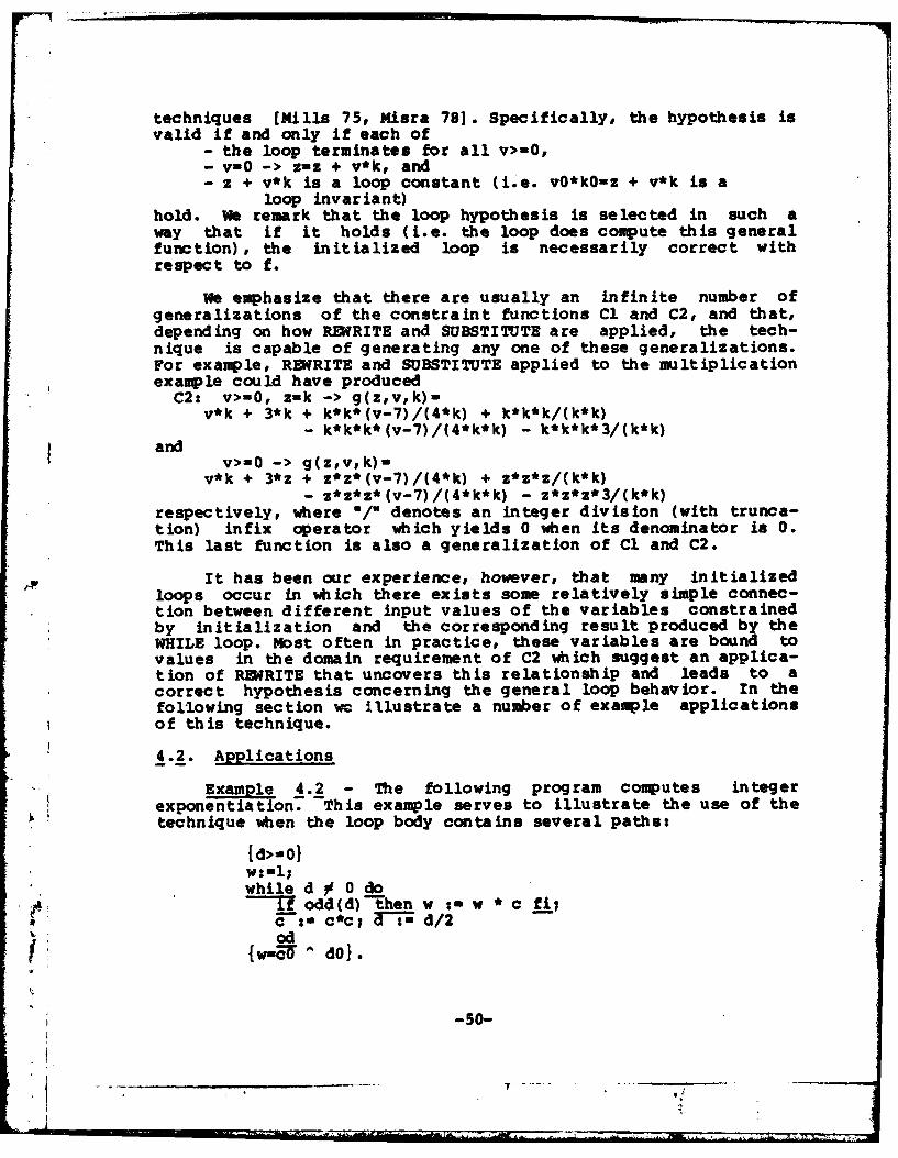
techniques [Mills 75, Misra 781. Specifically, the hypothesis isvalid if and only if each of

- the loop terminates for all v>-O,- v-0 -> z-z + v*k, and- z + v*k is a loop constant (i.e. vO*kO-z + v*k is a

loop invariant)hold. We remark that the loop hypothesis is selected in such away that if it holds (i.e. the loop does compute this generalfunction), the initialized loop is necessarily correct withrespect to f.

we emphasize that there are usually an infinite number ofgeneralizations of the constraint functions Cl and C2, and that,depending on how REWRITE and SUBSTITUTE are applied, the tech-nique is capable of generating any one of these generalizations.For example, REWRITE and SUBSTITUTE applied to the multiplicationexample could have produced

C2: v>-O, z-k -> g(z,v,k)-v*k + 3*k + k*k*(v-7)/(4*k) + k*k*k/(k*k)

- k*k*k*(v-7)/(4*k*k) - k*k*k*3/(k*k)and

v>-O -> g(z,v,k)-v*k + 3*z + z*z*(v-7)/(4*k) + z*z*z/(k*k)

- z*z*z*(v-7)/(4*k*k) - z*z*z*3/(k*k)respectively, where '/" denotes an integer division (with trunca-tion) infix operator which yields 0 when its denominator is 0.This last function is also a generalization of Cl and C2.

It has been our experience, however, that many initializedloops occur in which there exists some relatively simple connec-tion between different input values of the variables constrainedby initialization and the corresponding result produced by theWHILE loop. Most often in practice, these variables are bound tovalues in the domain requirement of C2 which suggest an applica-tion of REWRITE that uncovers this relationship and leads to acorrect hypothesis concerning the general loop behavior. In thefollowing section we illustrate a number of example applicationsof this technique.

4.2. Applications

Example 4.2 - The following program computes integerexponentiation. This example serves to illustrate the use of thetechnique when the loop body contains several paths:

{>-0}W:-l;

while d # 0 do•If odd(d)-then w :a w * c fi;

c : c*c; 3 d/2od

{WT - do}.

-50-

* _ _ _ _ _ _ _ _.__ _ - - -- .... .. ,..

The infix operator ' appearing in the postcondition represents

integer exponentiation. The first constraint function is easilyRECORDED:dO>-O, c=cO, d-dO, w-i -> g(Wc,d)-cO^dO

and SIMPLIFIES toCi: d>-O, w-i -> g(w,c,d)-c~d.

Since there exist two paths through the loop body, we will obtaintwo second constraint functions. The first of these deals withthe path which updates the value of w and is executed when theinput value of d is odd. The function is

dO>O, odd(dO), w-cO, c-cO*cO, d-dO/2 -> g(w,c,d)-cO^dOwhich SIMPLIFIES toC2a: d>-O, c-w*w -> g(w,c,d) -wA(d*2+1).

The function corresponding to the other loop-body path isdO>O, "odd(dO), w-l, c=cO*cO, d-dO/2 -> g(w,c,d)ucO^dO

and SIMPLIFIES tod>=O, w-1, SQUARE(c) -> g(w,c,d)=SQRT(c) ^ (d*2)

i.e.C2b: d>iO, w-1l, SQUARE(c) -> g(w,c,d)=c'd

where SQUARE(x) is a predicate which is TRUE iff x is a perfectsquare and SQRT(x) is the square root of the perfect square x.The term SQUARE(x) is necessary in the domain requirement sincethe unSIMPLIFIED function is only defined for values of c whichare perfect squares. Note that C2b is a subset of Cl and henceis of no additional help in characterizing the general loop func-tion. The heuristic suggested in REWRITE is to rewrite the func-tion expression w^(d*2+l) of C2a in terms of w, w*w (so as tointroduce c) and d. The peculiar nature of the exponent in thisexpression leads one to the equivalent formula w*((w*w)Ad).

Awl Applying SUBSTITUTE in C2a yieldsd>-O -> g(w,c,d)-w*(c^d).

This function is in agreement with (i.e. is a superset of) Cl andthus is a reasonable hypothesis for the general loop function.

In this example, the portion of C2 corresponding to theloop-body path which bypasses the updating of the initializeddata is a subset of Cl. Based on this, one might conclude thatsuch loop-body paths should be ignored when constructing C2. Con-sidering all loop-body paths, however, does increase the likeli-hood that an incorrect program could be disproved (at the timethe general loop function is being constructed) by observing aninconsistency between constraint functions C1 and C2. Forinstance, in the example, if the assignment to c had been written"c:-c*2*, the above analysis would have detected an inconsistencyin the constraints on the general loop function. Such an incon-sistency implies that the hypothesis being sought for the generalbehavior of the loop does not exist, and hence, that the programis, not correct with respect to its specification.

In the previous section, the reader may recall that awkward-* ness in disproving programs was offered as a disadvantage of a

*top down* approach to synthesizing g. However, it has been ourexperience that, as in the above instance, an error in the

-51-

* V

- -

program being considered often manifests itself as an incon-sistency between Cl and C2. Such an inconsistency is usually"easy" to detect and hence the program is "easy" to disprove.While it is difficult to give a precise characterization of whenthis will occur, intuitively, it will be the case provided thatthe "error" (e.g. c*2 for c*c) can be "executed" on the firstiteration of the loop.

Example 4.3 - The following program counts the number ofnodes lh a nonempty binary tree using a set variable s. Itdiffers from the previous example in that more than one variableis initialized. The tree variable t is the input tree whosenodes are to be counted. We use the notation left(t) andright(t) for the left and right subtrees of t respectively. Thepredicate empty(t) is TRUE iff t is the empty tree (i.e. contains0 nodes).

{ empty(t)}n :- 0; s : {t);while s { o

select and remove some element e from s;n := n + 1;if -empty( left(e)) then s :s U Ileft (e)} fi;if -empty(right(e)) then s :-s U lright(e)} fi0

{n-NODES(t)l

The notation NODES(t) appearing in the postcondition stands forthe number of nodes -in binary tree t. The first constraint func-tion is

Cl: "empty(t), n-0, s-,i -> g(n,s)-NODES(t).Rather than considering each of the four possible paths throughthe loop body individually, we abstract the combined effect ofthe two IF statements as the assignment

s :- s U SONS(e),where SONS(x) is the set of 0, 1 or 2 nonempty subtrees of x.Applying this, the second constraint function is

C2: "empty(t), n-1, s-SONS(t) -> g(njs)-NODES(t).We choose to REWRITE the function expression for C2 using therecursive definition that NODES(x) for a nonempty tree x is 1plus the NODES value of each of the 0, 1 or 2 nonepty subtreesof x. Specifically, this would be

l+SUM(xSONS(t) ,NODES (x))where SUM(A,B,C) stands for the summation of C over all A e B.Applying SUBSTITUTE in the obvious way yields

"empty(t) -> g(n,s)=n+SUM(x, s,NODES(x))which is in agreement with Cl and is thus a reasonable guess forthe general loop function g.

Two remarks are in order concerning this example. The firstdeals with the condition "empty(t) appearing in the domainrequirement of the obtained function. The reader may wonder, ift is not referenced in the loop (it is not in the argument list

-52-

p t

for g), how can the loop behavior depend on emptylt)? The answeris that it obviously cannot; the above function is simplyequivalent to

g(n,s)=n+SUM(x,s,NODES(x)).For the remainder of the examples of this section, we assume thatthese unnecessary conditions are removed from the domain require-ment of the constraint function as part of the SUBSTITUTE step.

As a second point, in Example 4.3 we encounter the casewhere the obtained function is, strictly speaking, too general,in that its domain includes "unusual" inputs for-7ich thebehavior of the loop does not agree with the function. Forinstance, in the example, the loop computes the function

g(n,s)-n+SUM(x,s,NODES(x))only under the provision that the set s does not contain theempty tree. This is normally not a serious problem in practice.One proceeds as before, i.e. attempts to push through a proof ofcorrectness using the inferred function. If the proof is suc-cessful, the program has been verified; otherwise, the charac-teristics of the input data which cause the verificationcondition(s) to fail (e.g. s contains an empty tree) suggest anappropriate restriction of the input domain (e.g. s contains onlynonempty trees) and the program can then be verified using thisnew, restricted function.

Example 4.4 (Gries 79] - Ackermann~s function A(m,n) can bedefined as foll7ows for all natural numbers m and n:

A(O,n) = n+lA(m+l,0) = A(m,l)A(m+l,n+l) - A(m,A(m+l,n)).

The following program computes Ackermann's function using asequence variable s of natural numbers. The notation s(1) is therightmost element of s and s(2) is the second rightmost, etc.The sequence s(..3) is s with s(2) and s(1) removed. We will use< and > to construct sequences, i.e. a sequence s consisting of nelements will be written <s(n), ... ,s(2),s(l)>.

{m>=O,n>-O)s :- <m,n>;while size(s) # 1 do

if s(2) 0 then s:"s(..3) < s( 1 )+l>

eseif s(1)-' then s:-s(..3) <s(2)-l,l>else s:=s(..3) s<s(2)-l,s(2),s(l)-l> fi

{s-ZX(m, n) >1

For this program, the first constraint function isCl: m>=O, n>-0, s-<m,n> -> g(s)=<A(mn)>.

The second constraint functions corresponding to the 3 pathsthrough the loop body are

C2a: m-0, n>-O, su<n+l> -> g(s)=<A(m,n)>

-53-

C2b: m>O, n -0, s-<m-l,l> -> g(s)-<A(m,n)>C2c: m>O, n >0, s=<m-l,m,n-l> -> g(s)-<A(m,n)>.

REWRITING these 3 based on the above definition of A yieldsm-O, n>-O, s-<n+l> -> g(s)-<n+l>m>O, n -0, s-<m-l,l> -> g(s)-<A(m-l,1)>m>O, n >0, s=<m-l,m,n-l> -> g(s)-<A(m-l,A(m,n-l))>.

SUBSTITUTING here yieldss=<s (I)> -> g(s)=<s(1)>s=<s(2),s(1)> -> g(s)-<A(s(2),s(1))>s-<s(3),s(2),s(l)> -> g(s)-<A(s(3),A(s(2),s(1)))>.

Note that the second of these functions implies Cl. The 3 seemto suggest the general loop behavior (where n>l)g(<s(n),s(n-l), ... ,s(l)>) =

<A(s(n),A(s(n-l), ... A(s(2),s(l)) ... ))>.

We remark that in the first 3 examples, the heuristicresulted in a loop function which was sufficiently general (i.e.the loop was closed for the domain of the inferred function).Example 4.4 illustrates that this does not always occur. Theloop function heuristic is helpful in the example in that it sug-gests a behavior of the loop for general sequences of length 1, 2and 3. Based on these results, verifier is left to infer abehavior for a sequence of arbitrary length.

Example 4.5 - Let v be a one dimensional array of length n>0which contains natural numbers. The following program finds themaximum element in the array:

m :- 0; i := 1;while i <- n do

7 m < v[i-then m := v i] fL;i :=i + 1fi

{m=GGEST (v)

The notation BIGGEST(v) appearing in the postcondition stands forthe largest element of v. The following constraint functions areobtained

Cl: m-0, i-1 -> g(m,i,v,n)-BIGGEST(v)C2: m-v[l1, i2 -> g(m,i,v,n)-BIGGEST(v).

Noticing the appearance of v[1] and 2 in C2, we REWRITEBIGGEST(v) in C2 as MAX(v[l],BIGGEST(v[2..n])), where MAX returnsthe largest of its two arguments, and v[2..n] is a notation forthe subarray of v within the indicated bounds. The generaliza-tion which suggests itself,g(m, i,v,n)-MAX(mBIGGEST(v[i..nl )),

agrees with Cl.Example 4.6 - If p is a pointer to a node in a binary tree,

let OST(p) e-the sequence of pointers which point to the nodesIin a postorder traversal of the binary tree pointed to by p. Thefollowing program constructs POST(p) in a sequence variable vsusing a stack variable stk. lb use the notation l(p) and r(p)

-54-

(w -A_ _

for the pointers to the left arnd right subtrees of the treepointed to by p. if p has the value NIL, POST(p) is the emptysequence. The variable rt points to the root of the input treeto be traversed.

p :- rt; stk := E4PTY; vs *. <>;while -(piNIL & atk-EMPTY) do

i? W~NIL thenstk <- p7* push p onto stk *p :- 1(p)

elsep <- stk /* pop stk *Vs s Vs p>p :r(p) fi

od{vs - POST(rt)1.

Up until now, we have attempted to infer a general loop functionfrom two constraint functions. Of course, there is nothing spe-cial about the number two. in this example, the Twconnection"between the initialized variables and the function values is notclear from the first two constraint functions and it proves help-ful to obtain a third constraint function. Functions Cl and C2correspond to 0 and 1 loop-body executions, respectively. Thethird constraint function C3 will correspond to 2 loop-body exe-cutions. We will use the notation (el, ... ,en) for a stack con-taining the elements el, o. ,en from top to bottom. The con-straint functions for this program areCl: p-rts stk*EMPTY, vsn(>

g (p, stk, vs) -POST (rt)C2: rt#NIL, p-l(rt), stk-(rt), vs->

g (p, stk, vs) -POST (r t)C3a: rt$dNIL, l(rt)#NIL, p-l(l(rt)), stkn(l(rt),rt), vs-<> -

g(p, stk,vs) -POST (rt)C3b: rt)&NIL, l(rt)-NIL, p-r(rt), stk-EIPTY, vs-<rt> ->

g (p, stk, vs) -POST (rt) .Note that there are two third constraint functions. C3a and C3bcorrespond to executions of the first and second loop-body paths(on the second iteration), respectively. There is only 1 secondconstraint function since only the first loop-body path can beexecuted on the first iteration. Using the recursive definition

b of POST, we REWRITE C2, C3a and C3b as follows:C2*: rtANIL, p-l(rt), stk-(rt), Vow<> ->

Ca:g(prstk,vs) -POST (1(rt)) 1jcrt>Ij POST(r(rt))C~':rt)6NIL, l(rt)INIL# p-l(l(rt)), stk-(1(rt),rt), vs-<> ->

g(p,stk,vs)-POBT(l(l(rt))) <l(rt)>tt POST(r(l(rt)))'I'Irt>II POST(r(rt))

g (p, atk, vs) -<rt> IIPOST Cr (r t)) .Applying SUBSTITUTE to each of C2*, C3a* and C3b'* suggestsstk-(el), vsu<" -> g(p,stk,vs):POST(p) IIecl> IPOST(r(el))stk-(el,e2), vs-<> -> g(p,stk,vs) POST(p) <el> IPOST(r(el))

<e2> JPOST(r(e2))

_51

stk=EMPTY -> g(p,stk,vs)=vslIPOST(p)respectively. The first 2 of these functions imply the followingbehavior for an arbitrary stack where vs has the value <>:stk-(el, ..., en), vs-<> -> g(p,stk,vs)

POST(p) 1I (<el>ll POST(el) I...Il<en>ll POST(en))and in combination with the last function, the general behaviorstkn(el, ..., en) -> g(p,stkvs) -

vs II POST(p) I (<el>11 POST(el) II...II<en>II POST(en))is suggested.

In this section we have illustrated the use of our techniqueon a number of example programs. The reader has seen that thesuccess of the method hinges largely on the way REWRITE is per-formed. hat guidelines can be used in deciding how to applythis step? The general rule given above is to identify the vari-ables that need to be introduced into the expression and then torewrite the expression using the terms to which these variablesare bound. For instance in Example 4.3, NODES(t) was rewrittenusing the terms 1 and SONS(t). Beyond this rule, however, thereader may have noticed an additional similarity in the wayRWERITE was applied in these examples. If f is the function oroperation the initialized loop program is intended to compute,each REWRITE step involved decomposing an application of f insome way. In Example 4.1, for instance, a multiplication opera-tion was decomposed into an addition and multiplication opera-tion; in Example 4.3, a NODES operation was decomposed into asummation and a number of NODES operations; in Example 4.5, aBIGGEST operation was decomposed into a MAX and a BIGGEST opera-tion. In Section 4.5 we will characterize this idea of decompos-ing the intended operation of the initialized loop program anddiscuss several implications of the characterization for the pro-posed technique.

In Example 4.6, we saw that the technique generalizes to theuse of three (and indeed an arbitrary number of) constraint func-tions. We have seen that each of these functions defines a sub-set of the general loop function g being sought. If the con-straint functions themselves are sufficiently general, it may bethat the first several of these functions, taken collectively,constitute a complete description of g. We consider this situa-tion in the following section.

j 4.3. Complete Constraints

The technique described above for obtaining a general loopfunction is "nondeterministic" in that the constraint functionsdo not precisely identify the desired function; rather they serveas a formal basis from which intelligent guesses can be made con-cerning the general behavior of the loop. Our belief is that itis often easy for a human being to fill in the remaining "pieces"of the loop function "picture" once this basis has been esta-

F blished.

-56-

(l

There exist, however, circumstances when the constraints doconstitute a complete description of an adequate loop function.Specifically, this description may be complete through the use ofone, two or more of the constraint functions. The significanceof these situations is that no guessing or "filling in the pic-ture" is necessary; the program can be proven/disproven correctusing the constraints as the general loop function. In this sec-tion we give a formal characterization of this circumstance.

Definition 4.1 - For some N > 0, an initialized loop is N-closed with respect to its specification f iff the union of theconstraint functions Cl,C2, ... ,CN is a function g such that theloop is closed for the domain of g. In this case, the con-straints Cl,C2, ... CN are complete.

Thus if a loop is N-closed for some N>0, the union of thefirst N constraint functions constitutes an adequate loop func-tion for the loop under consideration. Intuitively, the value Nis a measure of how quickly (in terms of the number of loopiterations) the variables constrained by initialization take on"general" values.

Example 4.7 - The following program

(b>-O}a :- a + 1;while b > 0 do

a : a +T;b : b-Iad

{a=aU'+ bO + 11

is 1-closed since the first constraint function isCl: bO>-0, a-aO+l, b-bO -> g(a,b)-aO+bO+l

which SIMPLIFIES tob>=O -> g(a,b)-a+b

and the loop is closed for the domain of this function. Thus C1by itself defines an adequate loop function.

Initialized loops which are 1-closed seem to occur rarely inpractice. Somewhat more frequently, an initialized loop will be2-closed. For these programs, the loop function synthesis tech-nique described above (using 2 constraint functions) is deter-ministic.

Example 4.8a - Consider the program

.

" -7

sum 0;Owhile seq # EMPTY do

sum :- sum + heal(seq)seq :a tail(seq)od

(sum-SIGMA(seqO) 1The notation SIGMA(seqO) appearing in the postcondition standsfor the sum of the elements in the sequence seqO. The program is2-closed since the second constraint function is

C2: seq0O#!MPTY, sum-head(seqO), seq-tail(seqO) -

g(sum, seq) -SIGMA(seqO)which SIMPLIFIES to

g (sum, seq) -sum+SIGMA(seq).The loop is trivially closed for the domain of this function.

Example 4.8b - As a second illustration of a 2-closed ini-t iali zed -loop, the following program tests whether a particularkey appears in an ordered binary tree.

success :- FALSE;while tree #d ILL & -success do

if namne(tree) =key then- success :- TRUEelseif name(tree) <key then tree :=right(tree)else tree :-left(tree) fi

{sucess - IN(key,treeo)1

The notation IN(key,tree0) is a predicate which is true iff keyP occurs in ordered binary tree treeO. This program is also 2-

closed. Note that the first constraint functionCl: success-FALSE, tree-tree0 ->

g (success, tree, key) -IN (key, treeG)SIMPLIFIES to

success-FALSE -> g (success, tree, key) -IN (key, tree).if we consider the first path through the loop body, the secondconstraint function is

C2: success-TRUE, tree0O'NIL, tree-tree0, key-name(tree) -

g(success, tree, key) -IN(key, treeO)wh ic h SIMPLI FIES to

succeuss*TRUE, treONIL, key-name(tree) -

g(success, tree, key) -IN(key, tree).Although the domain of the union of these two functions is some-what restricted, i.e.

I success, tree, key>((-success) MR (treelONIL & key-name (tree))))I,

the loop is nevertheless closed for this domain and hence theinitialized loop is 2-closed.

Example 4.8c - Consider the sequence of initialized loopsPl,P2,P3 ... defined an follows for each 1>0:

PI • {x>-0}x : x * I;while x > 0 do

x = x - -Ty "y + kod

{yp, "+ xO*I*k}.

For any I>O, the first I constraint functions for program PI areCl: xO>=0, xmxO*I, y=yo -> g(z,y,k)=y0+xO*I*kC2: xO>-l, x-x0*I-l, y-yO+k -> g(z,y,k)=y+xO*I*k

CI: xO>=I-l,x=x0*I-(I-i),y=y0+k*(I-1) -> g(x,y,k)=y0+xO*I*k.These SIMPLIFY to

x>=O, MI(x) -> g(x,y,k)-y+x*kx>=O, MI(x+l) -> g(x,y,k)=y+x*k

x>=0, MI(x+(I-1)) -> g(z,y,k)=y+x*kwhere MI is a predicate which is TRUE iff its argument is a mul-tiple of I. Since the union of these is the function

x>=O -> g(x,y,k)-y+x*k,and the loop is closed for the domain of this function, we con-clude that for each I>0, program PI is I-clo -- .

For many initialized loops which seem to occur in practice,however, there does not exist an N such that they are N-closedwith respect to their specifications. This means that no finitenumber of constraint functions will pinpoint the appropriate gen-eralization exactly; i.e. when applying the above technique inthese situations, some amount of inferring or guessing willalways be necessary. A case in point is the integer multiplica-tion program from Example 4.1. The constraint functionsClC2,C3, ... define the general loop behavior for z-0, z-k,z-2*k, ... etc. The program cannot be N-closed for any N sincewith input v=N+l, the last value of z will be (N+l)*k which isnot in the domain of any of these constraint functions.

As a final comment concerning N-closed initialized loops, itmay be instructive to consider the following intuitive view ofthese programs. All 1-closed and 2-closed initialized loopsshare the characteristic that they are "forgetful,0 i.e. theysoon lose track of how "long" they have been executing and lackthe necessary data to recover this information. This is due tothe fact that intermediate data states which occur after an arbi-

* trary number of iterations are indistinguishable from data states*which occur after zero (or one) loop iterations. To illustrate,

consider the 2-closed initialized loop of Example 4.8a which sumsthe elements contained in a sequence. After some arbitrarynumber of iterations in an execution of this program, suppose we

-59-

stop it and inspect the values of the program variables sum andseq. Based on these values, what can we tell about the historyof the execution? The answer is not too much; about all we cansay is that if sum is not zero then we know we have previouslyexecuted at least 1 loop iteration, but the exact number of theseiterations may be 1, 10 or 10000.

By way of contrast, again consider the integer multiplica-tion program of Example 4.1, an initialized loop we know not tobe N-closed for any N. Suppose we stop the program after anarbitrary number of iterations in its execution. Based on thevalues of the program variables z, v and k, what can we tellabout the history of the execution? This information tells us agreat deal; for example, we know the loop has iterated exactlyz/k times and we can reconstruct each previous value of the vari-able z.

Initialized loops which have the information available toreconstruct their past have the potential to behave in a "tricky"manner. By "tricky" here, we mean performing in such a way thatdepends unexpectedly on the history of the execution of the loop(i.e. on the effect achieved by previous loop iterations). Theresult of this loop behavior would be a loop function which was"inconsistent" across all values of the loop inputs and whichcould only be inferred from the constraint functions with consid-erable difficulty. We consider this phenomenon more carefully inthe following section; for now we emphasize that it is preciselythe potential to behave in this unpleasant manner that is lackingin 1-closed and 2-closed initialized loops and which allows theirgeneral behavior to be described completely by the first one ortwo constraint functions.

4.4. oTricky* Programs

The above heuristic suggests inferring g from two subsets ofthat function, C1 and C2. Constraint function C2 is of particu-lar importance since REWRITE and SUBSTITUTE are applied to thisfunction and it, consequently, serves to guide the generalizationprocess. C2 is based on the program specification f, the ini-tialization and the input/output behavior of the loop body on itsfirst execution. In any problem of inferring data concerningsome population b:esed on samples from that population, the accu-racy of the results depends largely on how representative thesamples are of the population as a whole. The degree to whichthe samp-e defined in C2 is is representative of the unknown gen-eral function we are seeking depends entirely on how representa-tive the input/output behavior of the loop body on the first loopiteration is of the input/output behavior of the loop body on anarbitrary subsequent loop iteration.

To give the reader the general idea of what we have in mind,consider the program to count the nodes in a binary tree in Exam-ple 4.3. If the loop body did something peculiar when, for

-60-

f..

example, the set s contained two nodes with the same parent node,or when n had the value 15, the behavior of the loop body on itsfirst execution would not be representative of its generalbehavior. By "peculiar" here, we mean something that would nothave been anticipated based solely on input/output observationsof its initial execution. An application of our heuristic onprograms of this nature would almost certainly fail since(apparently) vital information would be missing from Cl and C2.

Example 4.9 - Consider applying the technique to the follow-ing program which is an alternative implementation of the integermultiplication program presented in Example 4.1:

{v>=01z :- 0;while v # 0 do

if z=O then z := kelseif z=k then z = z * 2 * velse z -= z- k fi;v := v-1od

{z=vW*k.

The constraint functions C1 and C2 are identical to those for theprogram in Example 4.1 and we have no reason to infer a differentfunction g. Yet this function is not only an incorrecthypothesis, it does not even come close to describing the generalbehavior of the loop. The difficulty is that the behavior of theloop body on its first execution is in no way typical of its gen-eral behavior. This is due to the high dependence of the loop-body behavior on the input value of the initialized variable z.

We make the following remarks concerning programs of thisnature. Fi:st, our experience indicates that they occur veryrarely in practice. Secondly, because they tend to be quite dif-ficult to analyze and understand, we consider them *tricky" orpoorly structured programs. Thirdly, the question of whether the(input/output) behavior of the loop body on the first iterationis representative of its behavior on an arbitrary subsequentiteration is really a question of whether its behavior when theinitialized variables have their initial values is representativeof its behavior when the initialized variables have "arbitrary"values. Put still another way, the question is whether the loopbody behaves in a "uniform" manner across the spectrum of possi-ble values of the initialized data.

In practice, a consequence of a loop body exhibiting thisuniform behavior is that there exists a simply expressed connec-

* A.tion between different input values of the initialized data and+. the corresponding result produced by the WHILE loop. It is the

existence of such a connection which motivates the SUBSTITUTEstep above and which is thus a necessary precondition for a suc-cessful application of the technique. This explains its failure

' i -61-Lii_

in dealing with program. such as that in Example 4.9. We make nofurther mention of these "tricky" programs, and in the followingsection discuss an informal categorization of "reasonable" pro-grams and consider its implications for our loop function syn-thesis technique.

4.5. BU and TD o

In this section, we discuss general characteristics of manycommonly occurring iterative programs. These characteristics areused to suggest two categories of these programs. This categori-zation is of interest since the above heuristic for synthesizingloop functions is particularly useful when applied to initializedloops in one of these categories.

In solving any particular problem, it often makes sense toconsider certain instances of the problem as being "easier" or"harder" to solve than other instances. For example, with theproblem of sorting a table, the ease with which the sort can beperformed may depend on the size of the table, i.e. an instanceof the problem for a table containing N elements might be harderto solve than an instance of the problem for a table containingN-1 elements. Similarly, if the problem is multiplying naturalnumbers, a*b might be easier to solve than (a+l)*b. This notionof "easier" and "harder" instances of a problem is particularlyapparent for problems with natural recursive solutions. Thesesolutions solve complex instances in terms of less complexinstances and hence support the idea of one problem instancebeing easier to solve than another.

For the purpose of this discussion, we divide the data modi-fied by the initialized loop under consideration into two sec-tions: the accumulating data and the control data. The accumu-lating data is the specified output variable(s) of the loop. Theremaining modified data is the control data and often serves to"guide" the execution of the loop and determine the point atwhich the loop should terminate. Both the accumulating data andthe control data are typically (but not always) constrained byinitialization in front of the loop.

Example 4.10a - In the program" J' {n>-O}

z :- 1; t : 0'while t # n do

t :-t + _;

od:- *

the variable z is the specified output of the loop and is hencethe accumulating data. The other modified variable, t, is usedto control the termination of the loop and is the control data.

-62-

,rk"ML

In many cases, the control data can be viewed as represent-ing an instance (or perhaps several instances) of the problembeing solved. As the loop executes and the control data changes,the control data represents different instances of this problem.To illustrate, we can think of the control data t in the previousexample as a variable describing a particular instance of thefactorial problem. As the loop executes, the variable t takes onthe values 0, 1, ... , n, and these values can be thought tocorrespond to the problems 01, 11, ... ni.

Based on these informal observations, we characterize a BU(from the Bottom Upward) loop as one where the control data prob-lem instances are generated in order of increasing complexity,beginning with a simple instance and ending with the input prob-lem instance to be solved. In the execution of a BU loop, thecontrol data can be viewed as representing the "work" that hasbeen accomplished "so far." We consider the factoFral programib-ove to be a BU loop. At any point in time, the "work" so faraccomplished is tI and t moves from 0 (a simple factorialinstance) to n (the input factorial instance).

Conversely, we characterize a TD (from the Top Downward)loop as one where the control data problem instances are gen-erated in order of decreasing complexity, beginning with theinput problem instance and ending with a simple problem instance.In the execution of a TD loop, the control data can be viewed asrepresenting the "work" that remains to be done.

Example 4.10b - We consider the following alternative imple-Smentatlon of fa-torial to be a TD loop:

{n>-0z :- 1; t :- n;while t # 0 do

2 :s Z* t

t :t -1od{zs T}.

As before z and t are the accumulating and control data respec-tively. The variable t moves from n (the input factorialinstance) and ends with 0 (a simple factorial instance). Afterany iteration, the product n*(n-l)* ... *(t-l) has been accunw-lated, leaving ti as the "work" that remains to be done.

Example 4.11 - As an additional illustration, consider thefollowing three initialized loops which compute integer exponen-tiation:

-63-

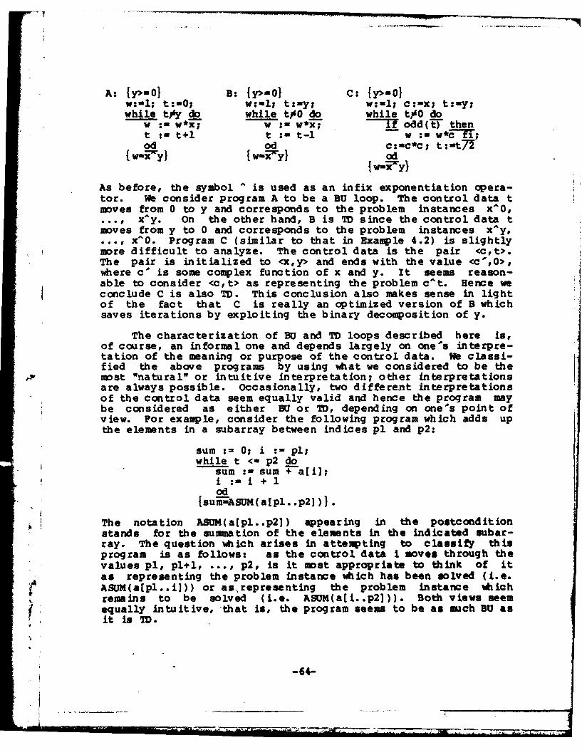
s-

A: 1y>-0) B: {y>inO} C: {y>-o1while ty do while tw0 do while t doW := w-' -- g:= w*x-- dd te

t :- t+l t := t-I - w :- w*c f;od Od c:mc*c; t:ut7{ w-'} I {~ }a

I W-rxy I lwi-ylyo

As before, the symbol ^ is used as an infix exponentiation opera-tor. We consider program A to be a BU loop. The control data tmoves from 0 to y and corresponds to the problem instances x^0,

x^y. On the other hand, B is TD since the control data tmoves from y to 0 and corresponds to the problem instances x^y,

, x^O. Program C (similar to that in Example 4.2) is slightlymore difficult to analyze. The control data is the pair <c,t>.The pair is initialized to <x,y> and ends with the value <c',0>,where c' is some complex function of x and y. It seems reason-able to consider <c,t> as representing the problem c~t. Hence weconclude C is also TD. This conclusion also makes sense in lightof the fact that C is really an optimized version of B whichsaves iterations by exploiting the binary decomposition of y.

The characterization of BU and TD loops described here is,of course, an informal one and depends largely on one's interpre-tation of the meaning or purpose of the control data. We classi-fied the above programs by using what we considered to be themost "natural" or intuitive interpretation; other interpretationsare always possible. Occasionally, two different interpretationsof the control data seem equally valid and hence the program maybe considered as either BU or TD, depending on one's point ofview. For example, consider the following program which adds upthe elements in a subarray between indices pl and p2:

sum :- 0; i :- pl;while t <- p 2 do

sum - sum + a[i];i :=i +1od

{su'-ASU(a[pl..p2] )}.

* The notation ASUM(a[pl..p2]) appearing in the postconditionstands for the summation of the elements in the indicated subar-ray. The question which arises in attempting to classify thisprogram is as follows: as the control data i moves through thevalues pl, pl+l, ... , p2, is it most appropriate to think of itas representing the problem instance which has been solved (i.e.ASM(a[pl..il)) or as representing the problem instance whichremains to be solved (i.e. ASBU(ati..p2])). Both views seemequally intuitive, that is, the program seems to be as much BU asit is TD.

-64-

As a final example, we refer back to the program in Example4.3 which counts the nodes in a binary tree. It is clear n andthe set variable s are the accumulating and control data respec-tively. Initially, s contains the tree whose nodes are to becounted; when the program terminates s is empty. In between, acontains various subtrees of the original tree. It seems naturalto view the set as containing progressively simpler and simplerinstances of the NODES problem since the trees in s consist offewer and fewer nodes as the loop executes. Thus we classify theprogram as a TD loop.

We have seen that the problem-solving method taken by a BUloop is one of approaching the general problem instance from somesimple problem instance. Of course, this problem-solving methodis reasonable only when there exists some technique whereby oneis guaranteed to "run into* the general problem instance. Ourview is that in many cases, such a convergence technique eitherdoes not exist or requires so much support that the BU approachis not practical. This appears to be particularly true for pro-grams dealing with sophisticated data types (i.e. something otherthan integers) and for programs requiring a high degree of effi-ciency in their number of iterations.

To help see this point of view, again consider the NODESprogram of Example 4.3. Previously we argued that this was a TDprogram. What would a BU program which computed the same func-tion look like? The following program skeleton suggests itself:

n := 0; tl :- "an empty tree";while tl # t do

"add a node-to tl to make it look more like t";n :- n + 1od

{n-NODES (t) }.

Here, the tree variable tl is the control data and it representsthe problem NODES(tl). The difficulty with this attempt at aprogram solution is the implementation of the modification of tl.Such a modification requires close inspection (i.e. a traversal)of t in order to move tl toward t. In light of this, it seemsmore reasonable to count the nodes of t while it is beinginspected and to dispense altogether with the variable tl.

As an illustration of another circumstance where the BUapproach seems unreasonable, the reader is encouraged to imaginea BU implementation of integer exponentiation which operates asefficiently as the exponentiation program C from Example 4.11.Again, a program skeleton suggests itself:

-65-

w %- 1; c :-?I d -=Ojwhile <c,d> yXy' do

c :- sqrt(c)if ? then

d := d * 2 + 1J w :- w * celse d :- d * 2 fi

{w-i yl.

Here, we are attempting to move the control data <c,d> toward<x,y> as fast as we moved it away from <x,y> in TD program C. Aswith the BU NODES program, the problem here is how to completethe program so as to achieve the desired effect. Our conclusionconcerning this program is that supplying an appropriate initialvalue for c and determining the proper loop-body path to be exe-cuted requires such complexity that this approach is not a feasi-ble alternative to program C.

In this section we have suggested two informal categories ofinitialized loop programs. We offered the opinion that theapproach taken in a BU program solution has rather limited appli-cability and that TD programs tend to occur more frequently inpractice. We feel that this characterization is useful as astudy of opposing problem-solving philosophies but our mainsource of motivation is to investigate the kinds of cornlyoccurring programs on which the loop function synthesis techniquedescribed above works well.

Consider applying this technique to a general TD program.In the second constraint function, the control data is bound to avalue which represents a slightly less complex instance of thegeneral problem being solved by the initialized loop. In prac-tice, the appearance of this value in the constraint functionsuggests the problem- Xecmo-- tion ber exploited by the pro-grammer in order to achieve the progr result. Applying thisdecomposition in REWRITE leads quite naturally to the desiredgeneral loop function.

Example 4.12 - Consider the TD factorial program from Exam-ple 4.M. 7Tfe second constraint function is

C2: n>O, z-n, t-n-l -> g(z,t)=nlThe control data t being bound to n-l suggests REWRITTING n1 asn*(n-l) I. This leads to the correct general loop function. Onthe other hand, consider the second constraint function for theBU factorial program from Example 4.10a:

C2: n>0, z-l, t=l -> g(zt,n)-nIHow can the expression ni be rewritten in terms of 1, 1 and n?To obtain the correct general function, the expression would haveto be rewritten as (l*nl)/(lI) which seems much less intuitiveVthan that required for the TD version. As another point of com-parison, consider the second constraint function for the TDexponentiation program B from Example 4.11:

i -66-

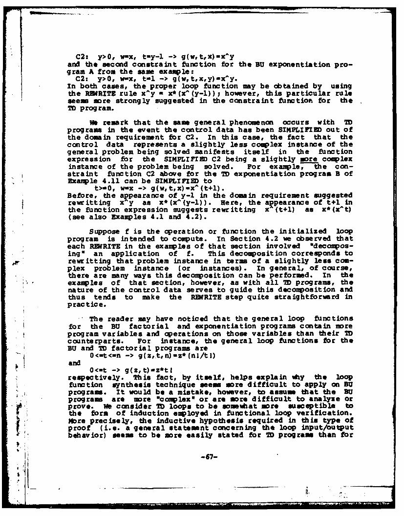
C2: y>O, w-x, t-y-1 -> g(w,t, x)lx'yand the second constraint function for the BU exponentiation pro-gram A from the same example:

C2: y>O, w x, t-l -> g(W,t,x,y) x^y.in both cases, the proper loop function may be obtained by usingthe RWRITE rule xAY - x* (XA (y-l)); however, this particular ruleseem more strongly suggested in the constraint function for theTD program.

Ne remark that the same general phenomenon occurs with TDprograms in the event the control data has been SIMPLIFIED out ofthe domain requirement for C2. In this case, the fact that thecontrol data represents a slightly less complex instance of thegeneral problem being solved manifests itself in the functionexpression for the SIMPLIFIED C2 being a slightly more complexinstance of the problem being solved. For example, the con-straint function C2 above for the TD exponentiation program B ofExample 4.11 can be SIMPLIFIE) to

t>-O, w-x -> g(w, t,x)-xA(t+l).Before, the appearance of y-l in the domain requirement suggestedrewritting x y as x*(x^(y-l)). Here, the appearance of t+l inthe function expression suggests rewritting x (t+l) as x*(x~t)(see also Examples 4.1 and 4.2).

Suppose f is the operation or function the initialized loopprogram is intended to compute. In Section 4.2 we observed thateach REWRITE in the examples of that section involved "decompos-ing" an application of f. This decomposition corresponds to

.rewritting that problem instance in terms of a slightly less com-plex problem instance (or instances). In general, of course,there are many ways this decomposition can be performed. In theexamples of that section, however, as with all TD programs, the

*1 nature of the control data serves to guide this decomposition andthus tends to make the RWRITE step quite straightforward inpractice.

The reader may have noticed that the general loop functionsfor the BU factorial and exponentiation programs contain moreprogram variables and operations on those variables than their TDcounterparts. For instance, the general loop functions for theBU and TD factorial programs are

and 0<-t<n -> g(z,.t,n)-z*(nl/tl)

0<-t -> g(z,t) z*tlrespectively. This fact, by itself, helps explain why the loopfunction synthesis technique seems more difficult to apply on BUprogram. It would be a mistake, however, to assume that the BUprogram are more *complex" or are more difficult to analyze orprove. Wb consider M loops to be somewhat more susceptible to

*the form of induction employed in functional loop verification.More precisely, the inductive hypothesis required in this type ofproof (i.e. a general statement concerning the loop input/outputbehavior) seems to be more easily stated for TD program than for

K-67-$ I

BU programs. On the other hand, BU programs seem somewhat moresusceptible to an inductive assertion proof. The inductivehypothesis required in this type of proof (i.e. a sufficientlystrong loop invariant) involves fewer program variables andoperations on those variables than the same type of hypothesisfor the corresponding TD loop. As an example the BU and TD fac-torial program have adequate loop invar ,ts 0<-t & zit! and0<-t<-n & z-ni/t! respectively.

In (Manna a Waldinger 70), the authors describe a programsynthesis technique and point out that their method produceseither of the above factorial programs depending upon which typeinduction rule the synthesizer is given to enploy.

4.6. Related Work

In [Basu & Misra 76, Misra 78, Misra 791, the authorsdescribe two classes of "naturally provable" programs for whichgeneralized loop specifications can be obtained in a determinis-tic manner. The technique proposed in this chapter sacrificesdeterminism in favor of wide applicability and ease of use. Ithandles in a fairly straightforward manner typical programs inthese two program classes (e.g. Examples 4.1-4.3) as well as anumber of programs which do not fit in either of the classes(e.g. Examples 4.4-4.6).

Due to the close relationship between loop functions andloop invariants (as discussed, for example, in Chapter 2), anytechnique for synthesizing loop invariants can be viewed as atechnique for synthesizing general loop functions (and viceversa). In this light, our method bears an interesting resem-blance to a loop invariant synthesis technique described in [Weg-breit 74, Katz a Manna 761. In this technique stronger and

* stronger *approximations" to an adequate loop invariant are madeby pushing the previous approximation back through the loop once,twice, etc.

* tBy way of illustration, consider the exponentiation programof Example 4.2. The loop exit condition can be used to obtain aninitial loop invariant approximation

d-O -> wmcOWdO.This approximation can be strengthened by pushing it back throughthe loop to yield

(d0 -> wucO'dO) & (d-1 -> w*c-cOAdO).In the analysis presented in Example 4.2, we obtained a value forthe generalized function specification for each of two differentvalues of the initialized variable w (i.e. I and SQRT(M)); herewe have obtained a *value* for the loop invariant we are seeking

bfor each of two different values of the variable which controls

the termination of the loop d. Applying the analysis in [Morris& Mgbreit 771, these loop invariant "values* can be translatedto constraint functions as follows:

duO- g(wcd)-w,

M ;**3 -68-

d,-l- g(w,c,d)-v*c.

Of course, the function expression w*c in the second constraintcan be rewritten w*(c*"l) ; SUBSTITUTING as usual suggests the gen-~eral loop function

g ( w, c, d) -w* (c^d).If we then add the program precondition as a domain restrictionon this function, the result is the same general loop functiondiscovered in Example 4.2.

We summarize the relationship between these two techniquesas follows. As the initialized loop in question operates on someparticular input, let X[0] , X[1], . ,X[N] be the sequence ofstates on which the loop predicate is evaluated (i.e. the loopbody executes N-i times). Of course, in X[0], the initializedvariables have their initial values, and in X[N], the loop predi-cate evaluates to FALSE. The method proposed in this chaptersuggests inferring the unknown loop function g from X[01, X[l],g(X[0]) and g(X[l]). The loop invariant technique describedabove, when viewed as a loop function technique, suggests infer-ring g from X[N], X[N-l], g(X[N]) and g(X[N-l]). Speakingroughly then, one technique uses the first several executions ofthe loop, the other uses the last several executions. Oneignores the information that the loop must compute the identityfunction on inputs where the loop predicate is FALSE, the otherignores the information that the loop must compute like the ini-tialized loop when initialized variables have their initialvalues.

Earlier we discussed "top down" and "bottom up" approachesto synthesizing g and indicated that our technique fit in the"top down" category. The technique based on the last severaliterations is a "bottom up" approach. It is difficult to care-fully state the relative merits of these two opposing techniques.In our view, however, there are a number of circumstances underwhich the technique based on the first several loop executionsseems more "natural" and easily applied. These examples includethe NODES program, the program to compute Ackermann's functionand the TD factorial program discussed above. The reason is thata critical aspect of the general loop function is the function

*computed by the initialized loop program (e.g. exponentiation inthe above illustration). In the technique based on the firstseveral iterations, this function appears explicitly in the con-straint functions. In the other technique, this information mustsomehow be inferred from the corresponding constraint functions(e.g. by looking for a pattern in these functions, etc.). Thisdifficulty is inherent in any "bottom up" approach to synthesiz-ing g.

In Chapter 3, we presented several guidelines for the syn-thesis of reductio hypotheses. Heuristic SHORTCUT of Theorem3.2 in that chapter is based on the observation that the program

A: Pl; B: Pl; P2;while B1 do while 31 do

--69-

P2 P2od o8

are equivale'nt on inputs which require at leIast on& loop itera-tion on program A. This is the underlying W7ILE loop propertythat is used to obtain constraint function C2 m the loop func-tion derivation technique described in this ikapter. Specifi-cally, C2 for the program A is exactly constraint function Cl forthe program B.

4.7. Discussion

In this chapter we have proposed a technique for derivingfunctions which describe the general behavior -f a loop which ispreceded by initialization. These functions c in be used in afunctional [Mills 75] or subgoal induction (Mrris & Wegbreit 77]proof of correctness of the initialized loop program. It is notour intention to imply that verification should occur after theprogramming process has been completed. There are, however, alarge number of existing programs which must be read, understood,modified and verified by "maintenance" personnel. We offer theheuristic as a tool which is intended to facilitate these tasks.

It has been argued [Misra 78] that the notion of closure ofa loop with respect to an input domain is fundamental in analyz-ing the loop. In Section 4.3, this idea is applied to initial-ized loop programs. The result is that a loop function g for aloop which is N-closed (for some N>O) can be synthesized in adeterministic manner by considering the first N constraint func-tions. Hence this categorization can be viewed as one measure ofthe "degree of difficulty" involved in verifying initialized loopprograms.

An interesting direction for future research is the develop-ment of a precise characterization of programs which are not"tricky" (as discussed in Section 4.4). Some results along thisline are described in Chapter 5 (see also [Basu 80]).

In Section 4.5 we discussed on an informal level the cppos-ing BU and TD problem-solving strategies and their correspondinginitialized loop realizations. We argued that the TD approachappeared to be more widely applicable and that, in practice, TDprogram seem to occur more frequently. Wb explained the success

b !of the proposed loop function creation technique on these pro-gram in term of an easily applied RWRITZ step. These resultsare offered to help support our view that the technique may beesployed successfully in a wide range of applications.

-70-

iI _ _ _ __ _ _ _ _

5. Analyzing Uniformly Implemented Loo]s

Consider the problem of proving/disproving a WHILE loopcorrect with respect to some functional specification f, i.e. frequires the output variable(s) to be some function of the inputsto the loop. If the loop precondition is weak enough so that thedomain of f contains the intermediate states which appear aftereach loop iteration (i.e. if the loop precondition is a loopinvariant), the loop is said to be closed for the domain of f.In Chapter 2 (Theorem 2.1) we saw that if the loop is closed forthe domain of its specification, there are two easily constructedverification conditions based solely on the specification, looppredicate and loop body which are necessary and sufficient condi-tions for the correctness of the loop (assuming termination) withrespect to its specification (Hills 75, Misra 78). If the loopis not closed for the domain of the specification function, ageneralized specification (i.e. one that implies the originalspecification) which satisfies the closure requirement must bediscovered before these verification conditions can be con-structed (this problem is analogous to that of discovering anadequate loop invariant for an inductive assertion proof [Hoare69] of the program).

We remark that the restricted specification often occurs inthe process of analyzing an initialized WHILE loop, i.e. one thatconsists of a WHILE loop preceded by some initialization code.This initialization typically takes the form of assignments ofconstant values to some of the variables manipulated by the loop.Examples include setting a counter to zero, a search flag toFALSE, a queue variable to some particular configuration, etc.It is clear that the initialized loop is correct with respect tosome specification if and only if the WHILE loop by itself iscorrect with respect to a slightly modified specification. Thisspecification has the same postcondition as the original specifi-cation and a precondition which is the original preconditiontogether with the condition that the initialized variables havetheir initialized values. Since the initialized variables willtypically assume other values as the loop iterates, the loop mostlikely will not be closed for the domain of this specification

* and a generalization of it will be necessary in order to verifythe correctness of the program.

Example 5.1 - The following program multiplies naturalnumbers using repeated addition:

{v>-O,k>-O}

while v > 0 doz : z +=0v vodf {z-v*k}.

-71-

- ° .o

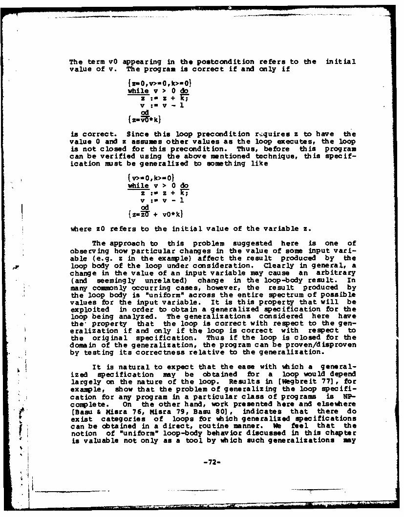
The term vO appearing in the postcondition refers to the initialvalue of v. The program is correct if and only if

{ z-O,v>-0,k>-0while v > 0 do

z : Z + TV :v-1od

{z-W*k}

is correct. Since this loop precondition r Lquires z to have thevalue 0 and z assumes other values as the loop executes, the loopis not closed for this precondition. Thus, before this programcan be verified using the above mentioned technique, this specif-ication mst be generalized to something like

{v>-0,k>-0}while v > 0 do

: Z +TV : v - 1od

{zzU + vO*k}

where zO refers to the initial value of the variable z.

The approach to this problem suggested here is one ofobserving how particular changes in the value of some input vari-able (e.g. z in the example) affect the result produced by theloop body of the loop under consideration. Clearly in general, achange in the value of an input variable may cause an arbitrary(and seemingly unrelated) change in the loop-body result. In

, rmany commonly occurring cases, however, the result produced bythe loop body is "uniform" across the entire spectrum of possiblevalues for the input variable. It is this property that will beexploited in order to obtain a generalized specification for theloop being analyzed. The generalizations considered here havethe property that the loop is correct with respect to the gen-eralization if and only if the loop is correct with respect tothe original specification. Thus if the loop is closed for thedomain of the generalization, the program can be proven/disprovenby testing its correctness relative to the generalization.

It is natural to expect that the ease with which a general-ized specification may be obtained for a loop would dependlargely on the nature of the loop. Results in (Wegbreit 771, forexample, show that the problem of generalizing the loop specifi-cation for any program in a particular class of programs is NP-complete. On the other hand, work presented here and elsewhere[Basu & Misra 76, isra 79, Basu 801, indicates that there doexist categories of loops for which generalized specificationscan be obtained in a direct, routine manner. We feel that thenotion of "uniform" loop-body behavior discussed in this chapteris valuable not only as a tool by which such generalizations may

-72-

______ ________

be obtained, but also as an attempt at a characterization ofloops which are susceptible to routine analysis, and hence inthis sense, easy to verify and comprehend.

The following section defines the necessary notation andterminology and then introduces the idea of a generalized loopspecification. Section 5.2 defines a uniformly implemented loopand states several implications of this definition for the prob-lem of generalizing a specification for such a loop. Theseresults are applied on several example programs in Section 5.3.In Section 5.4, a simplified procedure is suggested forproving/disproving a uniformly implemented loop correct withrespect to the obtained generalization. Finally, several guide-lines for recognizing uniformly implemented loops are presentedin Section 5.5.

5.1. Preliminaries

We will consider a verification problem of the form

{<z,y> e D(f))while B(<z,y>) do

z,y : h'(z,y,hA*(z,y)od

[<z,Y> - ft<zO,yO>).

In this problem, f is a data-state-to-data-state function. Thedata state consists of two variables, z and y. The terms zO andyO refer to the initial values of z and y respectively. Theeffect of the loop body is partitioned into two functions h' andh'* which describe the new values of z and y respectively.

The loop will be referred to as P. As before, the data-state-to-data-state function coputed by the loop (which, presum-ably, is not explicitly known) will be denoted [P]. Thus D([P])is the set of states for which P terminates. As a shorthandnotation we will use X for the state <z,y>, and H for the data-state-to-data-state function computed by the loop body, i.e.

H(X) - H(<z,y>) - <h*(z,y),h*'(z,y)>.

Suppose the loop is not closed for D(f) in that this setcontains only a restricted collection of values (maybe only one)of z and that other intermediate values of z occur as the loopiterates. The variable z will be called the key variable. Ourgoal here is to discover some more general specification f° whichincludes each of these intermediate values of the key variable inits domain. This generalization process (in one form or another)is necessary for a proof of correctness of the program under con-sideration.

Definition 5.1 - P is correct wrt a function f iff for all Xin D(f), [P) (X) !s-defined an TIT(X)-f(X).

-73-

Definition5.2 - A superset f' of f is a valid generaliza-tion of f iff if P is correct wrt f, then P is correct wrt f".

Note that the collection of supersets of f is partiallyordered by "is a valid generalization of. " The following defini-tion supplies the notation we will use to describe generaliza-tions of the specification function f.

Definition 5.3 - If S is a set of ordered pairs of datastates, f' is the extension of f defined by S iff f' is a func-tion and f' is the union of f i-d S.

Definition 5.4 - If g is the extension of f defined by(5.1) 1 (X,XK) I -B (X)}I,

then g is the base generalization of f.

Thus, if g is the base generalization of f, theng(Xl)=X2 <-> (f(Xl)=X2 OR (-B(Xl) & Xl=X2)).

Throughout this chapter, we wil- continue to use the functionsymbol g for the base generalization of f. We remark that gexists provided the union of f and (5.1) is a function, i.e. pro-v ided

x e D(f) & B(X) -> f(X)-Xholds. If this condition is not satisfied, P is not correct wrtf. Hence, if P is correct wrt f, the base generalization of fexists.

Theorem 5.1 - If g is the base generalization of f, then gis a valid generalization of f.

Proof - Suppose P is correct wrt f. We must show P iscorrect wrt g. Let X e D(g). If X e D(f), the loop handles theinput correctly by hypothesis. If X is not in D(f), we must haveB(X) and g(X)=X. Thus the program and g map X to itself and

thus are in agreement. Consequently P is correct wrt g, and g isa valid generalization of f.

The theorem utilizes the fact that the loop must necessarilycompute the identity function over inputs where the loop predi-cate is false. Combining this information with the programspecification f results in a valid generalization of f.

Definition 5.5 - A valid generalization f' of f is adequateif the loop is closed for D(fo).

The important characteristic of an adequate valid generali-zation f" is that it can be used to prove/disprove the correct-ness of P wrt the original specification f. Since the loop isclosed for D(f'), P can be proven/disproven correct wrt f" usingstandard techniques (Mills 72, Mills 75, Basu & Misra 75, Morris& Wegbreit 77, Wgbreit 77, Misra 781 . Specifically, P iscorrect wrt fV iff each of

(5.2) the loop terminates for all X e D(f')

-74-

...... ..

(5.3) X e D(f') & "B(X) -> (X)-Y(5.4) X e D(f*) & B(X) -> f'(X)-f'(H(X))

hold. If P is correct wrt f", then P is necessarily correct wrtany subset of f", including f. If P is not correct wrt f', thenby the definition of a valid generalization, P must not becorrect wrt f.

Example 5.2 - The following program tests whether a particu-lar key appears in an ordered binary tree.

{ success-FALSEIwhile tree # IULL & -success do

IT name(tree) = key then success := TRUEe-seif name(tree) < key then tree := right(tree)else tree := left(tree) fi

fsuc-ess = IN(treeO,key)}

The function IN(treeO,key) appearing in the postcondition is apredicate which means "the ordered binary tree treeO contains anode with name field key." The boolean variable success ischosen as the key variable since it is constrained to the valueFALSE in the input specification. Thus success plays the role ofz and the pair of variables <tree,key> correspond to y in theprogram schema discussed above. The specification function f is

f (<FALSE, tree, key>) = <IN(tree, key), tree', key**>where tree* and key' are the final values of the variables treeand key computed by the loop, respectively. That is, since thefinal values of these variables are not of interest in this exam-ple, we specify these final values so as to be automaticallycorrect. Using Theorem 5.1, a valid generalization of thisspecification is

g(<success, tree, key>) = if -success then<IN(tree, key) , tree*, key">

else if tree-NULL OR success then<success, tree, key>,

which is equivalent tog(<success,tree,key>)-<success OR IN(tree, key),tree', key'>.

In this example, the domain of the base generalization g off includes each value of the key variable, (i.e. FALSE and TRUE)and is thus adequate. Consequently, this generalization can beused to prove/disprove the correctness of the program.

In most cases, however, the heuristic suggested in Theorem5.1 is insufficient to generate an adequate generalization.Indeed, the base generalization is an adequate generalization

* only in the case when the sole reason for the closure conditionnot holding is the existence of potential final values of the keyvariable (e.g. TRUE in the example) which are absent from D(f).In order to obtain a generalization that includes general valuesof the key variable, an important characteristic of the loop bodywhich seems to be present in many commonly occurring loops will

-75-

be exploited.

5.2. Uniformly Implemented Loops

Definition 5.6 - Let P be a loop of the form describedabove. Let C bi a set, let Z be the set of values the key vari-able z may assume, and let Y be the set of values the remainingvariable(s) y may assume. Let

: C x Z -> Zbe an infix binary operator. The loop P is uniformly implementedwrt $ iff each of

(5.5) B(<z,y>) -> h* (c $ z,y) - c $* h* (z,y)(5.6) B(<z,y>) -> hAA(c $* z,y) - h" (z,y)(5.7) B(<z,y>) -> B(<c $* z,y>)

hold for all c e C, z e z and all y e Y.

Conditions (5.5) and (5.6) of this definition state that amodification to the key variable by the operation $* causes aslight but orderly change in the result produced by the loopbody. The change is slight because the only difference in theresult produced by the loop body occurs in the key variable.This difference is orderly because it corresponds precisely tothe same $" operation that served to modify the input value ofthe key variable. Condition (5.7) specifies that such a modifi-cation does not cause the loop predicate B to change from true tofalse.

As a shorthand notation we define the infix operator $ asc $ X = c $ <z,y> = <c $0 z,y>.

In this notation (5.5)-(5.7) are equivalent to(5.8) B(X) -> c $ H(X) - H(c $ X)

and(5.9) B(X) -> B(c $ X).

Example 5.3 - Consider again the program from Example 5.1which multipltei natural numbers using repeated addition:

{z-O,v>-O,k>-O}while v>O do

z : z k;V :m V - 1od

{z-_v-*k}.

Let z be the key variable. The pair <v,k> corresponds to thevariable y occurring in the above schema. The loop is uniformlyimplemented wrt +, where C and Z are both the set of naturalnumbers. Note that adding some constant to the input value of zhas the effect of adding the same constant to the value of z out-put by the loop body. Now consider the following alternativeimplementation of multiplication:

-76-

{z=O,v>=O, k>-O twhile v> 0 do

if W 0 & z-0 then z :- v -elsel! k-0 & z#0 t-e z :-z -1else z<k tEn z :- z + kelseif z-k then z :a z * 2 * velse z :a z k fi;V : V - 1cx5

* {zumvF*kl.

Again, let z be the key variable. This loop is not uniformlyimplemented wrt +. Intuitively, this is due to the high degreeof dependence of the loop-body behavior on the value of the keyvariable. The result of this dependence is that adding some con-stant to the value of z causes an unorderly change in the valueof z output by the loop body.

The reader may wonder if the second multiplication programabove might be uniformly implemented wrt some operation otherthan +. We remark that any loop is uniformly implemented wrt $A: C x Z -> Z defined by

c $' z - zfor all c e C and z e Z. For the purpose of our research, werule out such trivial operations, i.e. we require that for some ze Z, there exists some c e C such that

c $ z # z..P With this assumption, there does not exist an operation wrt which

the second of the above loops is uniformly implemented (or uorebriefly, the loop is not uniformly implemented). To see this,suppose the loop were uniformly implemented wrt $" • C x Z -> Z.Let cO and zO be some fixed elements of C and Z, respectively,which satisfy

cO $' zO # zO.Since (5.5) must hold for all c e C, z e Z and all y e Y, wechoose z=zO, c=cO and k-cO $' zO. Applying (5.5) gives

vO -> h*(cO $ zO,<v,cO $0 zO>)=cO $ h*(zO,<v,cO $ zO>)for all v. We consider 3 exhaustive cases based on the values ofcO and zO. First, suppose cO $ z- 0. Then we must have(since zO # 0)

v>O -> v-lcO $' (zO-1).Since this must hold for all v and the value cO $' (zO-l) isfixed by the original selection of cO and zO, this is a contrad-iction. Next, suppose cO zO # 0 and zO < cO $' zO. Then

v>O -> (cO $' zO)*2*v-cO $' (zO+(cO $* zO))for all v. Again, since the expression to the right of theequality sign is fixed and (cO $* zO)*2*v varies with differentvalues of v (cO $' zO is nonzero), this is a contradiction. Thethird case, where cO $' zO # 0 and sO > cO $' zO, leads to asimilar contradiction, and thus (5.5) does not hold. We concludethat the second multiplication program above is not uniformlyimplemented. That is, there does not exist a nontrivial modifi-cation that can be applied to the variable z which always results

-77-

in a slight and orderly change in the result produced by the loopbody.

The results presented here are based on the following lemmaconcerning uniformly implemented loops. The lemma describes theoutput of a uniformly implemented loop P for some modified inputc $ X (i.e. [P] (c $ X)) in terms of the output of the loop forthe input X (i.e. [P](X)) and the output of the loop for theinput c $ (P)(X) (i.e. [P](c $ [P1(X))).

Lemma 5.1 - Let P be uniformly implemented wrt $'. Then(5.10) X e D([P]) -> [P](c $ X)-[P](c $ [P1(X)).

Proof - We use induction on the number of iterations of P onX. For the base case of 0 iterations, [P] (X)-X, and the lemmaholds. Suppose it holds for all input data states X requiringn-l iterations where n > 0. Let Xl require n iterations. Sincen > 0, B(Xl) holds. By (5.9), B(c $ Xl). Note that H(Xl)requires n-l iterations on P; thus by the inductive hypothesis

[P(c $ H(Xl)) - [P](c $ [P)(H(xl))).Due to the uniform implementation this is

[P](H(c $ Xl)) - (P1Cc $ [P](H(Xl))).Using the loop property B(X) -> [P I (X) = [P I (H (X) ) on both sides weget

(PI C $ Xl) - [PJI(C $ [P I(Xl))Thus the inductive step holds and the lemma is proved.

The general idea behind our use of the lemma is as follows.Suppose the value [P] (X) is known for some particular X. I.e.suppose we know what the loop produces for the input X. In addi-tion, suppose that, given the result [P] (X), the quantity [P] (c $(P] (X)) is also known. With this information, we can then useLemma 5.1 to "solve" for the (possibly unknown) value [P] (c $ X).This additional information concerning the input/output behaviorof the loop can be used as an aid in constructing a valid gen-eralization of the specification f.

How can we find the value (P] X) and then the value [P] (c $[P] (X)) for some X? The key lies in assuming the loop P iscorrect wrt f. If P is not correct wrt f, any generalization off obtained by the technique will be a valid generalization bydefinition. Under this assumption, [P1(X) is known for X e D(f),i.e. x e D(f) -> [P] (X)-fX), and hence Lemma 5.1 implies(5.11) x e D(f) -> [P] (c $ X)-[PI(c $ f(X)).

Consider now the base generalization g of f defined in theprevious section. Recall that g is simply f augmented with the

*, identity function over the domain 4here the loop predicate B isfalse. Assuming as before that P is correct wrt f, P is thencorrect wrt g by Theorem 5.11 hence X e D(g) - [PI (X)-g(X).Thus (5.11) implies(5.12) X e D(f) a c $ f(X) e D(g) -> [PI(c $ X)-g(c $ f(X)).~Thus we can "solve" for the behavior of the loop on the input c$

-78-

i i I I I I II I /£

X, assuming X e Dlf) c $ fiX) e D(g) and P in correct wrt f.This suggests that if f" is the extension of f delsined by(5.13) 1 (c $ X,g(c $ f (X))) I X e D(f) rx c $ f (X) e D(g),

then VO is a valid generalization of f. Before giving a fo rmal1proof of this result, however, we first consider the question ofthe existence of such an extension of f. Specifically, it couldbe that for some c and X satisfying X e D(f) and c $ f(X) e D(g),that c $ X e D(f) and f(c $ X) # g(c $ f(X)). This woud implythat the extension of f defined by (5.13) does not exist. Thefollowing theorem states that this implies P is not correct wrtf.

Theorem 5.2 - Let P be uniformly implemented wrt $. Let gbe tie a l eneralization of f. If P is correct wrt f, thenthere exists a function fA which is the extension of f defined by(5.13), i.e.

{(c $ X,g(c $ f(X))) I x e D(f) . c $ f(X) e D(g)}.

Proof - Let f' be the function computed by the loop, i.e.[P]. Since P is correct wrt f, P is correct wrt g, and fC is asuperset of both f and g. By the lemma

fA(c $ X) = f,*(c $ fV(x))for all X e D(f). Since f*(X)-f(X) for X e D(f) and f*(X)-g(X)for X e D(g),

X e D(f) & c $ f(X) e D(g) -> f'(c $ X)=g(c $ f(X))holds. Thus (5.13) is a subset of f*. Since f is a subset ofC, the union of f and (5.13) is a subset of f". Hence thisunion is a function and is thus the extension of f defined by(5.13).

The following theorem is the central result presented here.The theorem formalizes the use of Lemma 5.1 in the manner sug-gested above, i.e. that the extension of f described in the pre-vious theorem is a valid generalization of the original specifi-cation.

Theorem 5.3 - Let P be uniformly implemented wrt $. Let gbe thile base generalization of f. If f* is the extension of fdefined by (5.13), i.e.

[(c $ X,g(c $ f(X))) I X e I(f) & c $ f(X) e D(g).,then f* is a valid generalization of f.

Proof - Suppose P is correct wrt f. We must show P iscorrect wrt f*. Let X e D(f*). If X e D(f), the loop handlesthe input correctly by hypothesis. If X is not in D(f), we musthave X - c $ Xl here X1 e D(f) and c $ f(Xl) 0 D(). By Lea5.1, [P] (X) - [PJ (c $ (P] (XI);. Since P is correct wrt f this is

A I[P (X) [PI (c $ f(Xl)). By Theorem 5.1, P is correct wrt 9.Using this, the equality can be written as [P](X) - g(c $ f(Xl)).By the definition of V this implies [P1(X) - fV(X). Thus P andf* are in agreement on the input X and consequently are in agree-ment on any input in D(f*). Hence P is correct wrt f and thusV is a valid generalization of f.

-79-

; I

The significance of Theorem 5.3 is that it provides a guide-

line for generalizing the specification of a uniformly imple-mented loop. If the loop is closed for the domain of the result-ing specification, the generalization can then be used toprove/disprove the program correct wrt the original specifica-t ion.

5.3.. Applications

In this section we illustrate the use of Theorem 5.3 with anumber of example programs which fall into either of twosubclasses of uniformly implemented loops. The subclassescorrespond to the two possible circumstances which can occur whenc $ f(X) of set definition (5.13) belongs to the set D(g) : thefirst, because -B(c $ f(X)), and, the second, because c $ f(X) eD(f). In each of these situations, the set definition (5.13)takes on a particularly simple form.

Definition 5.7 - A uniformly implemented loop satisfyingB(X) > (c $ X)

is a Typ A loop.

Observe that this condition along with (5.9) indicates thata Type A uniformly implemented loop satisfies

B(X) <-> B(c $ X),i.e. the value of the loop predicate B is independent of a changeto the data state by the operator $.

The intuition behind a Type A uniformly implemented loop isas follows. 1henever an execution of a Type A loop terminates(i.e. "B(X) holds) and the resulting data state is modified bythe operator $, the result is a new data state which, when viewedas a loop input, corresponds to zero iterations of the loop (i.e.the predicate B is still false despite the modification). Thisproperty is reflected in the following corollary.

iCorollary 5.3-1 Let P be a Type A loop. If fV is the ex-tens iono aEeiiea by

(5.14) { (c $ X,c $ f(X)) Xe D(f)},then f' is a valid generalization of f.

Proof - The proof consists of showing that (5.13) and (5.14)are equivalent for a Type A loop which is correct wrt f. ByTheorem 5.3, the corollary then holds. Let P be a Type A loopwhich is correct wrt f. A consequence of the correctness proper-ty is that "B(f(X)) for all X 6 D(f). Since P is a Type A loop,this implies B(c $ f(X)). Thus c $ f(X) 6 D(g) and g(c $

f(X))-c $ f(X). Consequently (5.13) and (5.14) are equivalent.

Of course, once a generalization fV has been obtained viaCorollary 5.3-1, there is no reason why that result cannot be fedback into the corollary to obtain a (possibly) further generali-zation f'" (using fo for f, f" for f*). This notion suggests

-_80-

the following general case of Corollary 5.3-1.

orllary 5.3-2 Let P be a Type A loop. If f is the ex-tension off eIiie3 by

{(cl$(c2$ ... (cn$X) ... ),cl$(c2$ ... (cn$f(X)) .. )Xe D(f) & n>-01 ,

then f* is a valid generalization of f.

Example 5.4 - Consider the following program to compute ex-ponentia tion.

{w-l,e>0,d>=O}while d > 0 do

Tf odd(d -then w := w * e fi;W-:- e*e ; T-/2od

{w-ef " dOlThe infix operator A appearing in the postcondition represents

integer exponentiation. In this example, w plays the role of thekey variable z, and the pair <e,d> corresponds to the variable y.We now consider wrt what operation the loop might be uniformlyimplemented. For any operation $', (5.7) holds (because w doesnot appear in the loop predicate) as does (5.6) (because thevalues produced in e and d are independent of w). Furthermore,(5.5) must hold for inputs which bypass the updating of w. Thusthe uniformity conditions reduce to

d > 0 & odd(d) -> (c V w) * e - c $" (w * e)Due to its associativity, it is clear the loop is uniformly im-plemented wrt *, where the sets C and Z are the set of integers.Since the key variable does not appear in the loop predicate, itis necessarily a Type A loop. The specification function here is

f(<l,e,d>) - <e ' d,eAd'>where e>0, d>m0 and e* and d are the final values computed bythe loop for the variables e and d. Applying Corollary 5.3-1, thefunction f* defined by

f*(<c*l,e,d>) - <c*(e " d),e*,d'>%here e>0 and d>-0 is a valid generalization of f. Since thisholds for all c, the definition of f* can be rewritten as

f*(<w,e,d>) - <w*(e " d),e',d">,where w is an arbitrary integer, e>0 and d>-0. The generaliza-tion fo is adequate and can thus be used to test the correctnessof the program wrt the original specification. Applying (5.2),(5.3) and (5.4) from above, these necessary and sufficient verif-ication conditions are

- the loop terminates for all e>O,, d>-O,-d=O-> w-w*(e ^ d), and-w*(e d) is a loop constant (i.e. eO A dO - w*(e A d)

is a loop invariant),respectively. In Section 5.4, we will discuss a simplificationof the last of these verification conditions which applies foruniformly mplemented loops.

i -81-

i

1 l5.5 iMsra 79] - The following program constructsthe preorder traversal of a binary tree with root node r. Theprogram uses a stack variable at and records the traversal in asequence variable seq.(seq-NULL, st-(r) /*stack st contains only the root node r*/}

while st .0 EMPTY dop <- at; /*pop-'he top off the stack*/seq :- seq I Iname(p); /*concatenate name of p onto seq*/if right(p) f NIL then at <- right(p) fi; /*push onto st*/Ef_ left(p) # NIL the-nst <- left(p) fiod

{sejPREOVR (r) }

The function PRORDNER(r) appearing in the postcondition is thesequence consisting of the preorder traversal of the binary treewith root node r. Let seq be the key variable. Similar reason-ing to that employed in the previous example indicates here thatthe loop is uniformly implemented wrt I, where the sets C and Zare the set of all sequences. It is a Type A loop. The specifi-cation function is

f(<ILL, (r)>) - <PREROER (r) ,st'>.* Again, the notation is used to represent the final values of

variables' that are of no interest. Applying Corollary 5.3-1 weobtain

f (<seq, (r)>) - <seqI PR D RD E ( r),st >as a valid generalization of f. In this case, fV is not adequatesince it does not specify a behavior of the loop for arbitraryvalues of the stack at. ft will return to this example afterconsidering another subclass of uniformly implemented loops.

Definition 5.8 - A uniformly implemented loop satisfyingB"(X) -> c s X e D(f)

is a Tye E loop.

The intuition behind a Type B uniformly implemented loop isas follows. 'henever an execution of a Type B loop terminates(i.e. "B(X) holds) and the resulting data state is modified bythe operator $, the result is a new data state which is a *valid'starting point for a new execution of the loop (i.e. this newstate is in D(f)). This property is reflected in the followingcorollary.

Corollarl 5.3-3 - Let P be a Type B loop. If f in the ex-tension of f defined by

(5.15) {(c $ X,f(c $ f (X) I x 6 D(f)},then f is a valid generalization of f.

Proof - The proof consists of showing that (5.13) and (5.15)are equivalent for a Type B loop which is correct wrt f. ByTheorem 5.3, the corollary then holds. Lot P be a Type B loopwhich is correct wrt f. A consequence of the correctness proper-ty is that "Bf(X)) for all X a D(f). Since P is a Type B loop,

-82-

I1this implies C $ f(X) D(f). Thus c $ f(X) 6 D(g) and g(c $f(X))-f(c $ f(X)). Consequently (5.13) and (5.15) areequivalent.

As before, a general case of this corollary can be statedwhich corresponds to an arbitrary number of its applications.

Corollary 5.3-4 - Let P be a Type B loop. If fV is the ex-tension of f defi3e by{(cl$(c2$( ... $(cn$X)...)),f(cl$f(c2$f( ... $f(cn$f(x) ... )))j|X S D(f) & n>-Othen fV is a valid generalization of f.

Example 5.5 (continued) - We now consider the problem offurther generalizig the derived specification in the previousexample. The variable for which the loop is not closed, st, willnow be the key variable. Consider an operation c $" at that hasthe effect of adding an element c to the stack st. Before beingmre precise about this operation, we consider how the loop bodyworks, and how its output depends on the value of the key vari-able at.

We observe that the loop-body behavior relies heavily on thecharacteristics of the node on the top of the stack. Consequent-ly, a modification c $* at to at which pushed a new node c ontothe top of st would not catse a slight and orderly change in theresult produced by the loop body and the uniformity conditions(5.5)-(5.7) would not hold. However, because the loop-bodybehavior seems to be independent of what lies underneath the topof the stack, we suspect the loop is uniformly implemented wrtADDUND , where C is the set of binary tree nodes, Z is the setA Dof stacks of binary tree nodes, and c ADDU .,ER at is the stackthat results from adding c to the bottom of st. Conditions(5.5)-(5.7) for this operation indicate that, indeed, this is thecase.

Let f be the generalization fV from the previous example.In keeping with the convention described above, since at is nowthe key variable, we will reverse the order in which the twovariables appear in the data state, i.e. we will write <st,seq>instead of <seq, st>.

The program is a Type B uniformly implemented loop sincest-EMPTY -> <c ADDUNDE st, seq> 6 D(f)

where c is a node of a binary tree, and specifically(5.16) st-EMPTY -> f(<c ADDUNI st, eq>)

Sst, seq PR3)N)t U(c) >.* Applying Corollary 5.3-4, if (r,cn, . ,cl) is an arbitrary

* stack (with r on top, ci on the bottom, n>-O)f'(<(r,cn, ... ,cl),Beq>) -f'(cl$(c2$( ... $(cn$<(r),seq>) ... ))) -f(cl$f(c2$f( ... $f(cn$f(<(r),seq>)) ... ))) -f(clsf(c2Sf( ... $f(cn$<st',pseqjjPR3DRNR(r)>) ... ))

-83-

4.t

P,

Recall that at** refers to the final value of at computed by theloop. The loop predicate indicates this wili always be the valueIM4TY. Hence (5.16) can be applied to this expression from In-side cut givingf (cl$f (c2$f(. <act',seq jPREDITCU(r) IPRNEN1MERcn) >...))

Cst',seql IPRBOM)U(r)IIPRUO1DER(cn) II ... ttPRODRDE(cl)>.Note that fV now defines a loop behavior for all sequences seqand nonempty stacks at. The base generalization of f* supple-mnents f with a behavior for the empty stack st and is thus anadequate generalization.

Examp~le 5.6 [Gries 79] - The following program computesAckeruiann-s nuiction using a sequence variable s of naturalnuubers. The notation s(l) is the rightmost element of s and

* s(2) is the second rightmost, etc. The sequence s(..3) is s with* s(2) and s(l) removed.

* { 5Is<IU,n) ,m>mO,n,-O1while size(s) #E 1 do

s(2)=O tiihn s:-s(..3) cs(l)+l>e Tseif s(l)-O then s:ins(..3) <s(2)-lpl>

*else s:-s(..3) C<s(2)-l,s(2),s(l)-l> fi

{s-ZA(m,n)>1

The function A(mn) appearing in the postcondit ion in Ackermann'sfunction. The specification function is

Let s be the key variable. As the loop-body behavior is indepen-dent of the leftmost portion of s, the loop is uniformly imple-me nted wr t Iwhere C is the set of natural numbers, Z is the setof noneepty sequences of natural numbersp and ci.a - <c> IIs. The

* program is also a Type B loop. By Corollary 5.3-4 (where nl),* tAf(cs(n),s(n-l), 9 ,(l)>)

f ( (n $ ( (n1) $(s(3)$<s(2),s(l)>) ... ))f(s(n)$f(s(n-l)$f( ... $f(s(3)$f(<s(2hrs(l)') ...f(s(n)$f(s(n-l)$f( ... $f(s(3)$<A(s(2),s(l)>') 0))-

*f(s(n)$f(s(n-l)$f( ... $f (<a(3)jA (9(2), s(l))) 0))

f(s(n)$f(s(n-l)$f( ... $<A(s(3)rA(s(2)ps(l)))> ...

<A(s(n) ,A(s(n-l), .. A(s(3),A(s(2)js(1).1) ...is a valid generalization of f. As in the previous example, thebase generalization of this function is adequate.

a 5.4. Simplifying the 'Iteration Conditionl'

IThe view of W~HILE loop verification presented here is one ofa two step process, the first step being the discovery of an ad*-Yr quate valid generalization V~ of the loop. specification f, thesecond being the proof of 3 basic conditions (i.e. (5.2)-(5.4))based on this generalization. We have seen that the uniform na-ture of a loop implesintation mey be used In the first step as an

_S4a.

*4 7

aid in discovering an appropriate generalization. In this sec-tion, we will exploit the same loop characteristic to substan-tially simplify one of the conditions which must be proven in thesecond step of this process.

The verification condition of interest is (5.4) above, i.e.X e D(f*) & B(X) -> f*(X)-fA(H(X)),

and is labeled the iteration condition in [Mtsra 781. This con-dition assures that as the loop executes, the intermediate valuesof X remain in the same level set of f*, i.e. the value of f' isconstant across the loop iterations. Previously we argued thatif P is uniformly implemented wrt $*, a change in the key vari-able by $* causes a slight but orderly change in the result pro-duced by H. Roughly speaking then, the behavior of H is largelyindependent of the key variable. If f' is chosen so as to beequally independent of the key variable, and the above conditionholds for X=<z,y> where y is arbitrary but the key variable z hasa specific simple value, we might expect the condition to holdfor all X. Such an expectation would be based on the belief thatthe truth or falsity of this condition would also be largely in-dependent of the key variable.

e formally characterize this circumstance in the followingdefin it ion.

Definition 5.9 - Let P be a loop of the form describedabove. A generalization f* of f is represented y f iff

(5.17) X e D(f ) & B(X) -> f (X)wf (E(X))

(5.18) X e D(f*) & B(X) -' fA(X)sfA(H(X)).

Thus if f* is represented by f, condition (5.17) can be usedin place of the iteration condition (5.18) in proving the loop iscorrect wrt f (and hence wrt f). The significance of this si-tuation is that the iteration condition can be tested with thekey variable constrained by initialization (as prescribed inD(f)). In practice, the result is one of having to prove a sub-stantially simpler verification condition.

The following theorems state that the use of Corollaries5.3-2 and 5.3-4 lead to generalizations which are represented bythe original specification.

Theorem 5.4 - Let P be a Type A loop. Suppose Uo is thevalid generalization of f defined in Corollary 5.3-2 and supposef' is adequate. Then f* is represented by f.

Proof - Suppose (5.17) holds and select some arbitrary X'from 7) satisfying B(X*). Thus there exists ol, ... , n e C,n>-O and X e D(f) such thatX's ci$(c2$( ... $(on $ X ...By the definition of a Type A loop, we must have B(X). Applyingthe definition of f" yields

~-85-

~I I__

f (X*)-cl$ (c2$(... $(Cn$f (X ).)wh ich is c$c$..$(o$fK(X

by (5.17) since B(X) holds. Since 1(X) e D(f*) (since fV is ade-quate), there exists dl, .... dm e C, m>-O, and Xl 8 D(f) suchth at

1(X) -dlS(d2$( ... $(dm$ XI .. )Futemo,f '(H(XM)dl$ (d2$(..$(dm$f(Xl)) ...))

Hence, continuing from abovefi.X')- cl$( ... $(cn$(dl$( ... $(dm$f(X)) ... ))..

~which is-f'(cl$( ... $(cn$ (dl$(...$ (dm$ X1.).)) .)

from the definition of f%. Thusf .(X') Mf A (cl$ ( ... $ (cn$H (X) ) .-

which is-f*(H(cl$( ... $(cn$ X).))

from the uniformity condition (5.8). Hencef "(X") -f D*(HMl )

and the theorem is proved.

Theorem 5.5 - Let P be a Type B loop. Suppose f" is thevalid g'eneraliation of f defined in Corollary 5.3-4 and supposef' is adequate. Then f'* is represented by f.

Proof - Suppose (5.17) holds and select some arbitrary X'from 5(-f ') satisfying B (X*). Thus there exists cl, #.. cn G C,n>-O0 and X e D(f) such that

X"- cl$(c2$( ... $(cn $ X ).))We make the assunption that 3(X). Otherwise, by the definitionof a Type B loop, the term cn $ X can be replaced by another X eD(f) . Since B (X1), th i.. nrocess can be continued until X" iswritten in the form above, with X e D(f) and B (X) . Applying thedefinition of f* yields

f'(X1*-f(cl$f(c2$f( ... $f(cn$f ( X )..)

whic is-f(cl$f(c2$f( ... $f(cn$f*(H(X))) ... ))by (5.17) since B(X holds. Since H(X) e D(f') (since f' is ade-quate), there exists dl, ... , dm e c, m>-O, and X1 e D(f) suchthatHM dl(2(..$d$l..)

Furthermore,f'*(H(X))-f(dl$f(d2$f( ... $f(dm$f(Xl)) ...))M.

Hence, continuing from abovef '(X)- f (cl$ f(. ...$f (cn$f(dl$f( ... $f (dm$f (Xl)) ...)).)

which is-fV (cl$( ... $(cn$(dl$( ... $(dm$X1) ...)..)

from the definition of f*. Thusf*(X*if'* (cl$( ... $ (cn$H (X))..)

wh ich ismf'((cl$( .$ (on$ X).)

from the uniformity condition (5.8). Hencef (X')-f(H (X'*)

and the theorem is proved.

Example 5.7 - Consider the exponentiation program of Example5.4. The generilization obtained from Corollary 5.3-2 is

f (<w,e,d>)-<w*(e d) ,e',d >,where e>O, d>-O. Since f" is represented by f, the iterationcondition corresponding to (5.17)

e>O & d>0 & odd(d) -> e d - e*((e*e)^(d/2)) &e>O & d>0 & "odd(d) -> e"d = l*((e*e)A(d/2))

can be used in place of that corresponding to (5.18)e>O & d>0 & odd(d) -> w*(e'd) = (w*e)*((e*e)^(d/2)) &e>O & d>0 & "odd(d) -> w*(e"d) = w*((e*e)^(d/2)).

The benefits of this simplification are more striking for morecomplex types of key variables. To illustrate, consider the pro-gram to compute Ackermann~s function in Example 5.6. ApplyingCorollary 5.3-4 to the base generalization g of f yields the gen-eralization defined by

n>l -> f'(<s(n),s(n-l),...,s(l)>) =<A(s(n) ,A (s(n-1),... ,A (s(3) ,A (s(2),s(l)))... ))>

andt fo(<s(1)>)-<s(1)>.

Since fO is represented by g, the iteration conditions(2)-O -> <A(s(2),s(l))>-<s(l)+l> &

s(2)#O & s(l)=O -> <A(s(2),s(1))>-<A(s(2)-l,l)> &s(2)#O & s(l)#O -> <A(s(2),s(l))>=<A(s(2)-l,A(s(2),s(l)-1))>

can be used in place ofn>l & s(2)0 -><A(s(n) ,A(s(n-1), ... ,A(s(3) ,A(s(2),s(l))) ...))>=<A(s(n) ,A (s(n-l) ,... ,A (s(3), s(1) +I)...))> &n>l & s(2)#O & s(l)=O -><A(s(n) ,A(s(n-l),... ,A(s(3),A(s(2),s(l )) )...))>=<A(s(n) ,A (s(n-l),... ,A (s(3) ,A (s(2)-l,l))...) ) >n>l & s(2)#O & s(l)#O-><A(s(n) ,A(s(n-l),... ,A(s(3) ,A (s(2),s(l))) ... ))><A(s(n),A(s(n-l),...,A(s(3),A(s(2)-l,A(s(2),s(l)-l))) ... ))>.

5.5; Recognizing Uniformly Implemented L

Although the problem of recognizing uniformly implementedloops is in general an unsolvable problem, the following guide-lines seem useful in a large number of situations.

Recognizing uniformly implemented loops can be viewed as asearch for an operation wrt which the loop is uniformly imple-mented. In practice, condition (5.5) is the most demanding con-straint on this operation. An effective strategy, therefore, isto use (5.5) as a guideline to suggest candidate operations.Conditions (5.6) and (5.7) must be proven to show the loop is un-iformly implemented wrt some particular candidate.

Often the modiric'ation to the key variable z in the loopbody is performe3 by a statement of the form

z := z # e(y)

-87-

..... .... .. ..

for some dyadic operation # and function e. In this case, condi-tion (5.5) suggests the loop may be uniformly implemented wrt #or some directly related operation. For example, if # is associ-ative, condition (5.5) holds for #. If # satisfies

(a # b) # c = (a # c? # b(e.g. subtraction), and an inverse #* of # exists satisfying

a # b = c <-> b V c - a(e.g. addition if # is subtraction), condition (5.5) holds for#V.

Another commonly occurring case is when the future values ofthe key variable z are independent of y, i.e.

h'(z,yl) - ho(z,y2)for all z, yl and y2. This situation arises most frequently whenz is some data structure which varies dynamically as the loopiterates. Typically, there exists some particular aspect or por-tion of the data structure (e.g. the top of a stack, the end of asequence, the leaf nodes in a tree) which guides its modifica-tion. A useful heuristic which can be employed in this cir-cumstance is to consider only operations which maintain (i.e.keep invariant) this particular aspect of the data structure.Selecting such an operation $* guarantees that the "change" ex-perienced by the data structure in the loop body will be indepen-dent of any modification $* and thus insures condition (5.5)holds.

In any case, recognizing uniformly implemented loops anddetermining the operation wrt which they are uniformly implement-ed is often farilitated if the intended effect of the loop body(as regards the key variable) is documented in the program sourcetext. Such documentation abstracts what the loop body does fromthe method employed to achieve this result and thus makesanalysis of the loop as a whole easier.

To illustrate, consider the following program to compute themaximum value in a subarray ai..n] of natural numbers:

{m-o}while i <- n do

m < a[ir-then m : a i fiL;

od{m=-AXIMI(a, iO,n) 1.

If the effect on m in the loop body were documented asm := MAX(m,a[i]),

its updating would be of the form m :- m # a[iJ and the heuristicdiscussed above could be employed to help determine that the loopis uniformly implemented wrt # a MAX.

-88-

AD-A113 141 MARYLAND UNIV COLLEGE PARK COMPUTER SCIENCE CENTER F/$ 9/2

AN INVESTIGATION OF FUNCTIONAL CORRECTNESS ISSUES.(U)

1982 D D DUNLOP F49620-80-C-0001UNCLASSIFIED CSC-TR-1135 AFOSR-TR-82-0263 NL

2IEFIEID

220E000E0[-

Q 2

~'1L60 1.0.0

" MICROCOPY RESOLUTION TEST CHART.

NATIONAL BUREAU Of STANDARDS-1963-A

'U ,...L

5.6. Related Work

The first work on generalizing functional specifications forloops appears in [Basu & Misra 76]. These results are refined in(Misra 78] and are studied in considerable detail in [isra 79].The major contribution of this research seem to be the identifi-cation of two loop classes or schemas which are "naturally prov-able." 7he first class is called the accumulating loop schemaand can be viewed as a (commonly occurring) special case of theType A loops discussed above. Specifically, a program in the ac-cumulating loop schema with associative binary operation $* inthe sense of [Basu & Misra 76] is necessarily uniformly imple-mented wrt $'* and meets the criterion for a Type A loop presentedabove.

The second of these classes is called the structured dataschema. A loop in this class is uniformly implemented wrt anoperator which adds an element to the data structure being pro-cessed in such a way that it is not the "next" element to be re-moved from the structure (e.g. recall the use of ADDUNDER in thetree traversal example). A loop in this class necessarily meetsthe criterion for a Type B loop presented above. The program tocompute Ackermann's function does not fit in the structured dataschema. We remark that the analysis presented in this chapterrelies on the loop body computing a function, i.e. it relies onthe loop body being deterministic. Consequently, the above com-ments do not apply to the non-deterministic structured data loops

/7 analyzed in [Misra 791.

In [Misra 791 the author states that the important codwonfeature between these program classes is that " ... they act upondata in a 'uniform' manner; changes in the input data lead tocertain predictable changes in the result obtained.0 7he workdescribed in this chapter can be viewed as an attempt to charac-terize this commonality and to generalize the work in [Misra 791based on this characterization.

More recently, [Basu 80] considers the problem of generaliz-ing loop specifications and uses the idea of a loop being "uni-form over a linear data domain." one difference between thiswork and cur notion of a uniformly implemented loop is that Basu

$ considers only program in the accumulating loop schema (in thesense of (Basu & Mist 761 without the closure requirement).More importantly, basu's idea of uniform behavior is based on thebehavior of the loop as a wlhole and seem to be largely indepen-dent of the loop body. Our approach relies solely on the charac-teristics of the loop body.

' Misra points out in [Misra 78, Hisra 791 that the iterationcondition for his structured data schema can be simplified in amanner similar to that presented herel our results show that thesame simplification can be applied to his accumnating loop eche-ma. Again, an appropriate view of the research described in this

-89-

chapter is one of generalizing this earlier work by investigatingthe theory which underlies these phenomenon.

5.7. Discussion

It is felt that a critical aspect of reading, understandingand verifying program loops is generalizing the behavior of aloop. over a restricted set of inputs to that over a more generalset of inputs. The view of this generalization process presentedin this chapter is one of ascertaining how changes in values ofparticular input variables affect the subsequent computation ofthe loop. This process is facilitated if these changescorrespond to particularly simple modifications in the resultproduced by the loop body.

Of course, the simplest possible modifications in the resultproduced by the loop body would be no modifications at all, i.e.the output of the loop body (and hence the loop) is completelyindependent of changes in these input variables. This situation,however, occurs rarely in practice since it implies that the in-put values of these variables serve no purpose in view of the in-tended effect of the loop. It is felt that the definition of auniformly implemented loop presented above is the "next best" al-ternative, and yet a large number of commonly occurring loopsseem to posseso this property. The definition states that interms of the execution of the loop body, prescribed changes inthe input value of the key variable affect only the final valueof the key variable; all other final values are independent ofthe change. Just as importantly, the modification caused in thefinal value of the key variable is necessarily the same as thechange in its corresponding input value. This property is analo-gous to that possessed by a function of 1 variable with unitslope in analytic geometry: increasing the input argument bysome constant causes the function value to be increased by exact-ly the same quantity. Ta'.en together, these factors account forthe pleasing symmetry between $ and H in condition (5.8).

Viewed as a verification technique for uniformly implementedloops, the procedure described above can be thought of astransforming the problem of discovering the general loop specifi-cation into the problem of discovering the operation with respectto which the loop is uniformly implemented. Clearly, this is ofno benefit if the latter is no easier to solve than the former.In many cases, however, it seem that simple syntactic checks aresufficient for identifying this operation. For example, in thetree traversal program, the fact that the loop body does not testthe stack for emptiness (Basu a IKisra 761 is a sufficient condi-tion for the loop being uniformly implemented with respect to

L ADENR.

It is felt that the notion of uniformly Implemented loopsmay have an application in the program development process.Specifically, when designing an initialized loop to cosute so

-90-

A

function, the programr should attempt to construct the loop Insuch a way that it is uniformly Implemainted with respect to noweasily stated operation. out work Indicates that thee loops aresusceptible to a rather routine form of analysis. Turthermors,implementing a loop in a uniform fashion requires mintaining acertain amunt of independence between program variables (orperhaps portions of program variables In the case of structures)and -a simple dependence between the Input/output values computedby the loop body. Such program are desirable since the earnwith which a loop can be understood depends largely on the com-plexity of the Interactions and interconnections among programvariables. ft remrk that the question of whether a given pro-gram is "well structured" has been viewed largely as a svtacticissue (e.g. use of a restricted set of control structures)VF woffer the definition of a uniformly Implemnted loop as an at-tempt at a characterization of a semantically veil structuredprogram.

44,

6. Sumary and Concluding Remarks

The purpose of this research has been an investigation of anumber of issues involved with the application of the functionalcorrectness methodology. In Chapter 2, we defined a functionalcorrectness technique and addressed the issue of the strategy em-ployed in decomposing composite program in the proof process.

Chapters 3-5 dealt largely with the issue of verifying pro-gram containing loops with undocumented or inadequate intendedfunctions. In Chapter 3, the idea of a reduction hypothesis wasintroduced. The use of a reduction hypothesis in a proof ofcorrectness eliminates the need for the intended loop function.As an alternative approach, a heuristic procedure for construct-ing intended loop functions was described in Chapter 4. Finally,in Chapter 5, a class of loops was described for which inadequateintended loop functions can be extended or generalized in a sys-tematic manner.

The most promising directions for future research seem tostem from the results presented in Chapter 5. %bile each uni-

formly implemented loop we have studied does exhibit a "reason-able" form of behavior, there do exist "reasonable" initializedloop programs which do not satisfy our definition. This situa-tion invariably occurs when initialized data is used in an in-direct manner (e.g. as an array index or pointer). A characteE---zation of uniform loop behavior with respect to indirect datawould serve as a useful complement to the results described in

1Chapter 5.

A second direction for future research is the development ofa program design/implementation methodology based on the uniform-ly implemented loop. At the point of designing an initializedloop program, the methodology would suggest the programmer firstformulate an appropriate operation, and then proceed to detailthe loop in a way which insured that it was uniformly implementedwith respect to that operation. We argued previously that uni-formly implemented loops are "well structured" program; such amethodology might be a valuable contribution to what has com tobe known as "structured programming."

-92-

7K

7. References

[Basili a Noonan 801Basili, V. R. and Noonan, R. 3. A Comparison of the Az-iomatic and Functional Models of Structured Programming,IBID Transactions on Software Snoineerilg, Vol. 83-6, Sept.

[Basu 80]Basu, S. A Note an Synthesis of Inductive Assertions, 1331Transactions on Software Enagineering, Vol. 83-6, Jan. l1317

Cflasu & Misra 751Basus. S.* and Misra, J. Proving Loop Prog ram, 1333 Transac-tions on Software Engineering, Vol. S3-l, Mareglr7, pp

(Basu a Misra 761Basu, S. K. and Misra, J. Some Classes of Naturally Prov-able Programs, Proc. 2nd International Conf. an Software

SSan Francico, Oct. 1976, pp. 400-10E

[Dijkstra 761Dijkstrar E. W. A Discipline of Programming, Prentice-Hall,1976.

[Ellozy 81]Ellozy, H. The Determination of Loop Invariants for Pro-gram with Arrays, IEEE Transactions on Software Engineer-Lng, Vol. SE5-7, Marc h7MfllT~p.I"'F_6.

(Floyd 671Floyd, R. W. Assigning Meanings to Program, Proceiigq ofa Symposia in Applied Mathematics, 19, 1967, pF 932.7

Gries 9. Is Sometime Ever Better Than Alway?, Transactions*on Prog mp Languages, and Systems, Vol. I, Oct17jp

[Hoare 69]Hare, C. A. R. An Axiomatic Basis for Computer Program-ming, CACZ4, Vol. 12, Oct. 1969, pp. 576-583.

(Katz & Manna 731Katz, S. and Manna, Z. A Heuristic Approach to Program Vo-

* rification, Proc. 3rd Int. Joint Conf. Axtificial Intell.rStanford, CA IM7, pp. SW-FSIT-

* [Katx AManna 761Katz, S. and Manna, Z. Logical Analysis of Program,. QWMVol. 19, April 1976p pp. 188-206.

ii -93-

(King 801King, J. Program Correctness: On Inductive AssertionMethods, IEEE Transactions on Sotftware Engineering, Vol.S3-6, SeptrT!O pp. 45M79.

(Linger, Hills & Witt 791Linger, R. C., Mills, R. and Witt, B. I. Structured Pro-gramming Theory and Practice, Addison-Wesley 7W.

(McCarthy 621McCarthy, 7. Towards a Mathematical Science of Computation.In: Popplewell, C.M. (ed.): Proc. IFIP Congress 62, North-Holland, Amsterdam, 1963, pp. T MS.-

[McCarthy 63]* I McCarthy, J. A Basis for a Mathematical Theory of Computa-

tion. In: Brafford, P., and Hirschberg, D. (eds.): CopProgramming and Formal Systems, Amsterdam, North Holland,

(Manna 71]Manna, Z. Mathematical Theory of Partial Correctness, J.Computer System Sci.,, Vol. 5, June 1971, pp. 239-253.

* (Manna & Pnueli 70]Manna, Z. and Pnueli, A. Formalization of Properties ofFunctional Programr, JACK, Vol. 17, July 1970, pp. 555-569.

[Manna a Waldinger 70]Manna, Z. and Waldinger, R. Towards Automatic Program Syn-thesis, Stanford Artificial Intelligence Project, Memo AIM-127, July 1970.

[Mills 7 21Mills, H. D. Mathematical Foundations for Structured Pro-gramming, ZEN Federal Systeim Division, PSC 72-6012, 1972.

[Mills 751mills, H. D. The New Math of Computer Programming, CRMVol. 18, Jan. 1975, pp. 43-48.

[Misra 77]Misra, J. Prospects and Limitations of Automatic AssertionGeneration for Loop Progra, SIAN 71. Comput.,, Vol. 6,, Dec.1977, pp. 718-729.-

[Misra 781t Kisra, J. Some Aspects of the Vearification of Loop Computa-

tions, 1333 Transactions on Software Engineering,, Vol. 83-4,Nov. 197spp 78-486

(misra,~ J. Systematic Verification of Simple Loops, t~iver-

-94-

sity of Texas ftchnical Report TR-97, March 1979.

[Morris a Webreit 77]Morris, J. H. and lbgbreit, B. Subgoal Induction, CUMVol. 20, April 1977, pp. 209-222.

[Strachey 641Strachey, C. Towards a Formal Semantics. In: Steel, To 3.,Jr. Co(d.): Pbrual Language Desciption ng M for Coan-

~~ ,,Proc. IFIPW~kn Conf f1964Yst uNort Ho1inTI66, pp. 198-220.

[Vsgbreit 74]Wgbreit, D. The Synthesis of Loop Predicates# CM,# Vol.17, Feb. 1974, pp. 102-112.

[Wstgbreit 771Negbreit, B. Complexity of Synthesizing Inductive Asser-tions,r JACH, Vol. 24, July 1977, pp. 504-512.

-95--