AN INTUITIVE METHOD FOR HILBERT CURVE CODING...A Hilbert curve (also known as a Hilbert...

$: AN INTUITIVE METHOD FOR HILBERT CURVE CODING...A Hilbert curve (also known as a Hilbert space-filling curve) is a continuous fractal space-filling curve first described by the German$
http://www.ijccr.com

VOLUME 1 ISSUE 3 MANUSCRIPT 11 NOVEMBER 2011

1

AN INTUITIVE METHOD FOR HILBERT CURVE CODING

Sasmita Mishra

Asst.Professor,

Department of Computer Science & Engineering,

Indira Gandhi Institute of Technology, Dhenkanal, Sarang

Odisha, India

Abstract

Hilbert curves can be generated by using L-System concept. A theoretical intuitive method is

suggested for manipulating the Hilbert space filling curve for simple coding to one dimension.

Our method is aimed to code the Hilbert curve simply by observing the base Hilbert curve as

generated. By simple observation one can code the Hilbert curve easily. The present work has

been mainly inspired by vertex labeling algorithms found in literature [1].

Key words: Hilbert curve, L-System, spacefilling curve

1.0 Introduction

A Hilbert curve (also known as a Hilbert space-filling curve) is a continuous fractal space-

filling curve first described by the German mathematician David Hilbert in 1891, as a variant of

the space-filling curves discovered by Giuseppe Peano in 1890. The Hilbert curve (Figure 1.1)

in particular appears to have useful characteristics (see for example: [2], [3], [4], [5], [6]).



2

However, it is widely considered to be tricky to work with. Abel and Mark [2] found the Hilbert

ordering to be very promising compared with a number of other orderings in certain application

domains, but the major weakness remains the lack of inexpensive algorithms to evaluate the

key of a cell or sub quadrant from its coordinates and vice versa. Nulty [17], working with

geometric range searching problems, noted that the Hilbert curve has excellent clustering

properties, but found it less convenient than the N-Curve or the Sierpinski curve. Laurini and

Thompson [8] found the Hilbert and Peano curves to be \more robust that is better performers

over a range of requirements, in spatial information systems. But, in the case of the Hilbert

curve, it is quite complex to get keys. The sequence of recursive Hilbert curves was discovered

by the mathematician David Hilbert about 100 years ago in order to answer the Space Filling

Curves Problem. In its simplest version, this problem asks if there exists a continuous function

from the unit interval [0, 1] that maps onto the unit square in the plane. The answer is yes and

the sequence of Hilbert curves gives a constructive definition of the function. To obtain the

function, one must “pass to the limit” as the level N of recursion goes to infinity. Hilbert curves

became well known in the computer science community because Nicklaus Wirth used them as a

key example of recursion in his fundamental text [2].

Because it is space-filling, its Hausdorff dimension is 2 (precisely, its image is the unit square,

whose dimension is 2 in any definition of dimension; its graph is a compact set homeomorphic

to the closed unit interval, with Hausdorff dimension 2). Hn is the nth approximation to the

limiting curve. The Euclidean length of Hn , i.e., it grows exponentially with n, while at the same

time always being bounded by a square with a finite area.



3

Certain space filling curves may not be given adequate attention, because of perceived difficulty

or simply unfamiliarity. Indeed, empirical evidence suggests that researchers do tend to stick

with the few well-known curves.

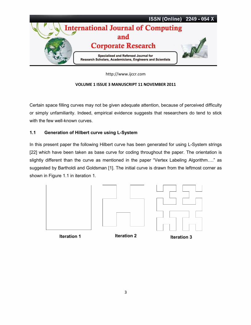
1.1 Generation of Hilbert curve using L-System

In this present paper the following Hilbert curve has been generated for using L-System strings

[22] which have been taken as base curve for coding throughout the paper. The orientation is

slightly different than the curve as mentioned in the paper “Vertex Labeling Algorithm….” as

suggested by Bartholdi and Goldsman [1]. The initial curve is drawn from the leftmost corner as

shown in Figure 1.1 in iteration 1.

Iteration 1

Iteration 2

Iteration 3



4

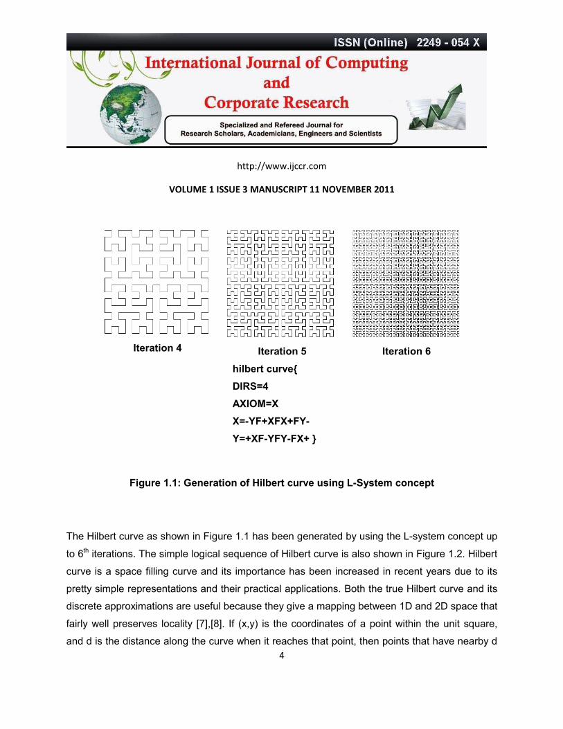
Iteration 4

Iteration 5

Iteration 6

hilbert curve{

DIRS=4

AXIOM=X

X=-YF+XFX+FY-

Y=+XF-YFY-FX+ }

Figure 1.1: Generation of Hilbert curve using L-System concept

The Hilbert curve as shown in Figure 1.1 has been generated by using the L-system concept up

to 6th iterations. The simple logical sequence of Hilbert curve is also shown in Figure 1.2. Hilbert

curve is a space filling curve and its importance has been increased in recent years due to its

pretty simple representations and their practical applications. Both the true Hilbert curve and its

discrete approximations are useful because they give a mapping between 1D and 2D space that

fairly well preserves locality [7],[8]. If (x,y) is the coordinates of a point within the unit square,

and d is the distance along the curve when it reaches that point, then points that have nearby d



5

values will also have nearby (x,y) values. The converse can't always be true. There will

sometimes be points where the (x,y) coordinates are close but their d values are far apart. This

is inevitable when mapping from a 2D space to a 1D space. But the Hilbert curve does a good

job of keeping those d values close together much of the time. So the mappings in both

directions do a fairly good job of maintaining locality.

Because of this locality property, the Hilbert curve is widely used in computer science. For

multidimensional databases, Hilbert order has been proposed to be used instead of Z order

because it has better locality-preserving behavior [8]-[11]. Given the variety of applications, it is

useful to have algorithms to map in both directions.

Figure 1.2: Generation of Hilbert Curve in simple steps

We offer a new approach, based on vertex-coding, for generating algorithms for the Hilbert

curve. This approach leads to simple procedures that involve no complex mathematical or

geometric operations. These procedures are also quite flexible. This is important since many

common geometric models are composed of irregular figures.



6

2.0 Organization of the paper

This paper is organised as follows.

The Section 1.0 discusses briefly about the concept behind Hilbert curve and highlights some of

practical application area in the field of computer science particularly in database. Section 1.1

elaborates simple method to generate Hilbert curve. The next section puts forth the survey

about the work done so far to find out the motivation and objective. Section 4 comprehensibly

discusses about the proposed indexing method in a lucid manner. The finally Section 5.0

concludes with future scope.

3.0 Survey

This survey aims at summarizing the literature relevant to R-trees. Space filling curves,

functions that continuously map the unit interval on to a bounded region of higher dimension,

have stimulated increasing interest in recent years due to their pretty representations and their

use in practical applications [5], [17].The Hilbert R-tree is a hybrid structure based on R-trees

and B+-trees [14]-[20]. Actually, it is a B+-tree with geometrical objects being characterized by

the Hilbert value of their centroid. Thus, leaves and internal nodes are augmented by the largest

Hilbert value of their contained objects or their descendants, respectively. For an insertion of a

new object, at each level the Hilbert values of the alternative nodes are checked and the

smallest one that is larger than the Hilbert value of the object under insertion is followed. In

addition, another heuristic used in case of overflow by Hilbert R-trees is the redistribution of

objects in sibling nodes. In other words, in such a case up to s siblings are checked in order to

find available space and absorb the new object. A split takes place only if all s siblings are full

and, thus, s+1 nodes are produced. This heuristic is similar to that applied in B*-trees, where



7

redistribution and 2-to-3 splits are performed during node overflows [18],[12],[21]. According to

the authors’ experimentation, Hilbert R-trees were proven to be the best dynamic version of R-

trees as of the time of publication. However, this variant is vulnerable performance-wise to large

objects.

4.0 Motivation

The present research is aimed at query processing and compression of large database system.

Particularly the resulted techniques may be used in range query processing and compression in

the telecom sector databases to reduce the disk spaces. In this paper an easier method is

suggested for coding of Hilbert spacefilling curve without mathematical complexities.

4.1 Suggested Intuitive Approach

Figure 1.2 shows an alternate way to illustrate the Hilbert curve, in which the line segments of

Figure 1.1 have been replaced by arcs. This is slightly different than the idea given in the paper

found from literature [1]. The arc notation conveys more information, since it (broadly) indicates

how space is ordered within each cell. Loosely speaking, the arcs are meant to show that the

curve enters each cell at a vertex, visits every point in the cell, exits at a different vertex, then

enters the next cell and so on.



8

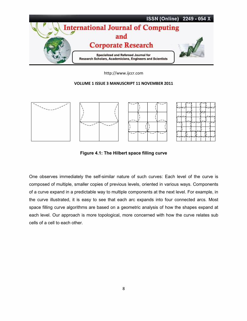
Figure 4.1: The Hilbert space filling curve

One observes immediately the self-similar nature of such curves: Each level of the curve is

composed of multiple, smaller copies of previous levels, oriented in various ways. Components

of a curve expand in a predictable way to multiple components at the next level. For example, in

the curve illustrated, it is easy to see that each arc expands into four connected arcs. Most

space filling curve algorithms are based on a geometric analysis of how the shapes expand at

each level. Our approach is more topological, more concerned with how the curve relates sub

cells of a cell to each other.



9

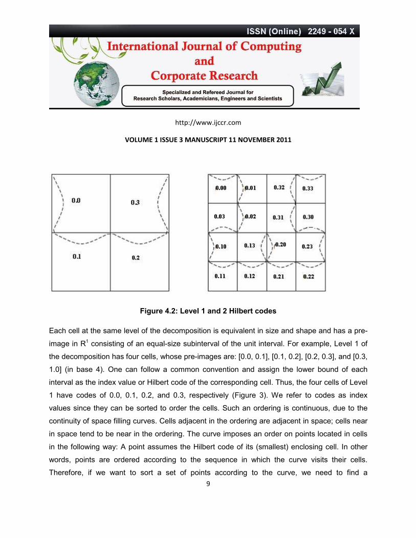
Figure 4.2: Level 1 and 2 Hilbert codes

Each cell at the same level of the decomposition is equivalent in size and shape and has a pre-

image in R1 consisting of an equal-size subinterval of the unit interval. For example, Level 1 of

the decomposition has four cells, whose pre-images are: [0.0, 0.1], [0.1, 0.2], [0.2, 0.3], and [0.3,

1.0] (in base 4). One can follow a common convention and assign the lower bound of each

interval as the index value or Hilbert code of the corresponding cell. Thus, the four cells of Level

1 have codes of 0.0, 0.1, 0.2, and 0.3, respectively (Figure 3). We refer to codes as index

values since they can be sorted to order the cells. Such an ordering is continuous, due to the

continuity of space filling curves. Cells adjacent in the ordering are adjacent in space; cells near

in space tend to be near in the ordering. The curve imposes an order on points located in cells

in the following way: A point assumes the Hilbert code of its (smallest) enclosing cell. In other

words, points are ordered according to the sequence in which the curve visits their cells.

Therefore, if we want to sort a set of points according to the curve, we need to find a



10

decomposition in which each point is located in a different cell, and then the ordering of the

points is established by their Hilbert codes.

We convert from a point in R2, to its Hilbert code (in R1), at a given precision, by finding a

sufficiently small cell enclosing the point. We are indifferent to the exact position of the point

within the cell. If we later want to recover the coordinates of a point, we will have to choose

some point within the enclosing region. With care, this can be performed multiple times without

loss of precision.

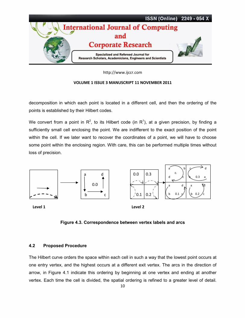
Figure 4.3. Correspondence between vertex labels and arcs

4.2 Proposed Procedure

The Hilbert curve orders the space within each cell in such a way that the lowest point occurs at

one entry vertex, and the highest occurs at a different exit vertex. The arcs in the direction of

arrow, in Figure 4.1 indicate this ordering by beginning at one vertex and ending at another

vertex. Each time the cell is divided, the spatial ordering is refined to a greater level of detail.

a d

0.0

b c

0.0 0.3

0.1 0.2

a b c d

d c b 0.3 a

a d a d

b 0.1 c b 0.2 c

Level 1 Level 2

0.



11

Our approach encodes cell vertices in sequence, to indicate the order in which regions of the

cell are visited by the curve. The vertex where the curve enters the cell is labeled ‘a’. The vertex

where the curve exits the cell is labeled ‘d’. The intermediate vertices are labeled, in order, ‘b’

and ‘c’.

The curve notation is a kind of shorthand for the vertex labels. Figure 4.3 shows how the

systems correspond. The arc notation is more visually appealing and reveals the spatial

ordering at a glance. In addition to its vertex labels, each cell has a base 4 Hilbert code between

0 and 1 indicating its place in the cell ordering. An observation now leads us to the labeling

approach to space filling curve algorithms referring to nothing more than the Hilbert codes and

vertex information (labels and coordinates) of a cell; we can generate the Hilbert codes and

vertex information of all of its sub cells.

The labeling process is summarized in Figure 5. At the top level, the Hilbert code is initialized to

`0:', and the vertices are labeled. At the next level, the square region is divided into four

equivalent square sub cells. The Hilbert code of each cell is updated by right-appending a digit

as follows: `0' for the cell containing vertex a; `1' for the cell containing vertex b; `2' for the cell

containing vertex c; `3' for the cell containing vertex d.

The new vertices are labeled in accordance with the basic Hilbert curve flow pattern. It is

very helpful to refer to the arc diagrams in determining the details of vertex relabeling. As an

example, we examine how the vertices in cell 0.0 (containing vertex a) are updated. Recall that

an arc enters a cell at vertex a, exits at vertex d, and the remaining vertices are labeled, in

sequence, c and d. We refer to the vertices of cell 0.0 as: anew, bnew, cnew, and dnew. By

observation (Figure 5), the arc enters cell 0.0 at vertex a, and exits at a vertex on the midpoint



12

of edge (a, b). Following the curve in sequence, vertex bnew is located at the midpoint of edge

(a,d), and vertex cnew is at the midpoint of edge (a; c). This leads to the following update rules for

cell 0.0.

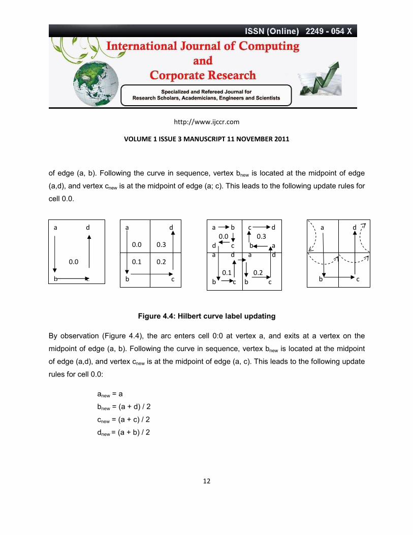
Figure 4.4: Hilbert curve label updating

By observation (Figure 4.4), the arc enters cell 0:0 at vertex a, and exits at a vertex on the

midpoint of edge (a, b). Following the curve in sequence, vertex bnew is located at the midpoint

of edge (a,d), and vertex cnew is at the midpoint of edge (a, c). This leads to the following update

rules for cell 0.0:

anew = a

bnew = (a + d) / 2

cnew = (a + c) / 2

dnew = (a + b) / 2

a d

0.0

b c

a d

0.0 0.3

0.1 0.2

b c

a b c d

0.0 0.3

d c b a

a d a d

0.1 0.2

b c b c

a d

b c



13

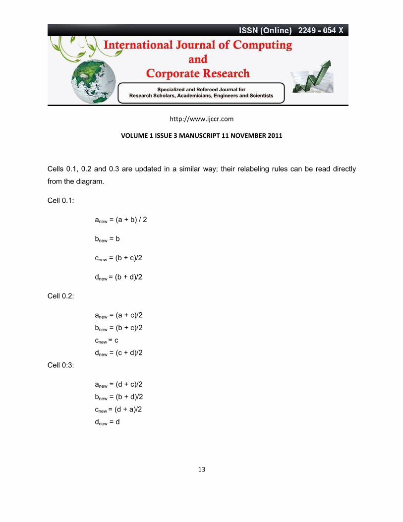
Cells 0.1, 0.2 and 0.3 are updated in a similar way; their relabeling rules can be read directly

from the diagram.

Cell 0.1:

anew = (a + b) / 2

bnew = b

cnew = (b + c)/2

dnew = (b + d)/2

Cell 0.2:

anew = (a + c)/2

bnew = (b + c)/2

cnew = c

dnew = (c + d)/2

Cell 0:3:

anew = (d + c)/2

bnew = (b + d)/2

cnew = (d + a)/2

dnew = d



14

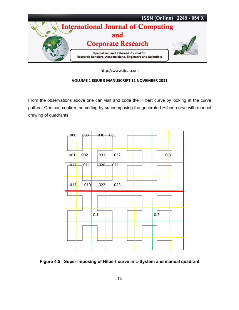
From the observations above one can visit and code the Hilbert curve by looking at the curve

pattern. One can confirm the coding by superimposing the generated Hilbert curve with manual

drawing of quadrants.

Figure 4.5 : Super imposing of Hilbert curve in L-System and manual quadrant

.000 .003 .030 .031

.001 .002 .031 .032 0.3

.012 .011 .020 .021

.013 .010 .022 .023

0.1 0.2



15

The above Figure 4.5 can directly be used for coding of curves. The topmost left corner cell is

coded as .000. The first quadrant has been coded and has been shown in the Figure 4.5

4.3 Summary of Hilbert curve labeling procedure

Step 1: Initialization.

We initialize the vertex labels of a square bounding region, so that the entry vertex of an arc is

labeled a, the exit vertex is labeled d, and the intermediate vertices are labeled in order b and c.

We assign Hilbert code '0.' to the region (Figure 4.4).

Step 2: Iterative step, I: Finding Hilbert codes of sub cells.

To create the next level of the decomposition, we divide the square into four sub squares, by

adding one edge from the midpoint of edge (a, b) to the midpoint of edge (c, d), and another

edge from the midpoint of edge (b, c) to the midpoint of edge (a,d). We first update the codes of

each of the four subcells as follows. The subcell containing vertex a is the first visited by the

curve, so we right-append the digit '0' to the code of its supercell. Following the path of the

curve, we right-append the digit '1' for the subcell containing vertex b, '2' for the subcell

containing c, and '3' for the subcell containing d.

Step 3: Iterative step, II: relabeling vertices of subcells.

Each arc expands into four arcs, one in each new subcell; we relabel vertices in such a way that

each new arc progresses from vertex a to d within its cell, with the intermediate vertices labeled,

in order, b and c. Vertices already labeled a, b, c and d do not change. The thirteen new

vertices

are labeled as detailed above (and in the figure).



16

Step 4: Finalization.

Continue the iteration steps until sufficient precision is reached.

Therefore, given initial vertex information and index value of a square region, creating iterates of

decomposition according to the Hilbert curve is a purely mechanical process. It can proceed

with no additional information, and no need to further analyze the geometry. By recursively

applying this procedure, we may label cells of the decomposition to any depth.

4.4 Computing a pre-image of a point in R2

We wish to convert from a point in a square bounding region to its corresponding Hilbert code. A

point located in a square region takes the Hilbert code of its smallest enclosing cell. A point can

be coded to a desired precision by enclosing it in a small enough regions and we can find an

arbitrarily small enclosing square by preceding to the necessary depth in the hierarchical

decomposition. The result is a labeled cell around the point, and a base 4 code on the interval

[0,1]. In determining the code, we need only label one sub square at each level; that is, we just

traverse the sequence of nested sub cells in which the point falls. Therefore the amount of work

required is proportional to the precision of the result. Summarizing the procedure to find a

Hilbert code of a point (refer to Figure 4.5):

1. Initialization.

Given a point P in a square bounding region, label the four vertices of the region a, b, c and d

(insequence), and initialize the Hilbert code of P to '0:'.



17

2. Iteration.

Divide the current enclosing square (a, b, c, d) into four equivalent sub squares.

If P is nearest vertex a, then update its Hilbert code by right-appending the digit '0', and update

vertex labels as follows:

anew = a

bnew = (a + d)/2

cnew = (a + c)/2

dnew = (a + b)/2

If P is nearest vertex b, right-append '1' to its code, and update labels as follows:

anew = (a + b)/2

bnew = b

cnew = (b + c)/2

dnew = (b + d)/2

If P is nearest vertex c, right-append '2' to its code, and update labels as follows:

anew = (a + c)/2

bnew = (b + c)/2

cnew = c

dnew = (c + d)/2

If P is nearest vertex d, right-append '3' to its code, and update labels as follows:

anew = (d + c)/2

bnew = (b + d)/2

cnew = (d + a)/2



18

dnew = d

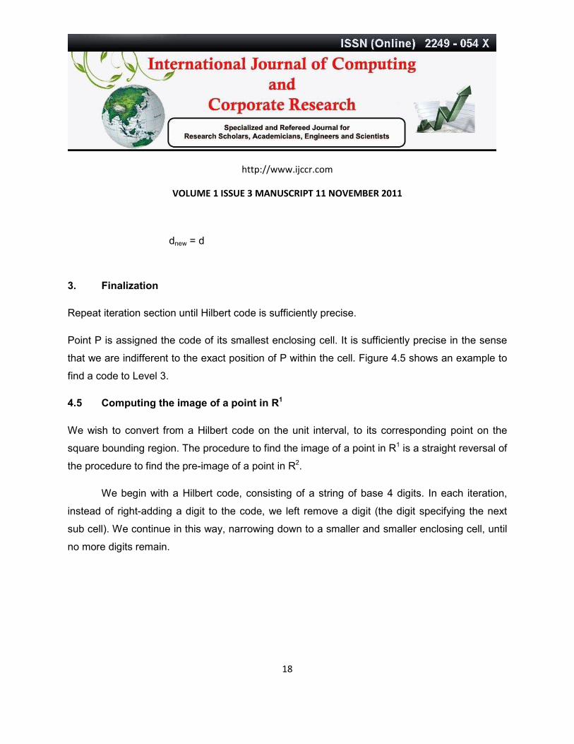
3. Finalization

Repeat iteration section until Hilbert code is sufficiently precise.

Point P is assigned the code of its smallest enclosing cell. It is sufficiently precise in the sense

that we are indifferent to the exact position of P within the cell. Figure 4.5 shows an example to

find a code to Level 3.

4.5 Computing the image of a point in R1

We wish to convert from a Hilbert code on the unit interval, to its corresponding point on the

square bounding region. The procedure to find the image of a point in R1 is a straight reversal of

the procedure to find the pre-image of a point in R2.

We begin with a Hilbert code, consisting of a string of base 4 digits. In each iteration,

instead of right-adding a digit to the code, we left remove a digit (the digit specifying the next

sub cell). We continue in this way, narrowing down to a smaller and smaller enclosing cell, until

no more digits remain.



19

Figure 4.6: Hilbert curve: Pont P is coded to Level 3

We are left with a square cell (a, b, c, d), and we choose our point from this region according to

some rule, such as: Take the average of the vertices. We label just one sub square at each

level of the subdivision. Therefore, the amount of work required is proportional to the precision

of the result (that is, the length of the Hilbert code). We briefly summarize the procedure:

1. Initialization.

Given a Hilbert code and a square bounding region, label the vertices a, b, c and d.

2. Iteration.



20

Divide the current square cell into four equivalent sub squares, as in the procedure to find the

code of a point. Remove the first digit r to the right of the decimal point from the Hilbert code. If r

= 0 then the sub cell containing vertex a becomes the current cell. If r = 1 then the sub cell

containing vertex b becomes the current cell. If r = 2 then the sub cell containing vertex c

becomes the current cell. Otherwise, r = 3 and the sub cell containing vertex d becomes the

current cell.

Relabel as in the labeling and point coding procedures.

3. Decision.

If no digits remain, then we are done. Otherwise, continue with the Iteration step.

Point P is assigned coordinates based on the final enclosing cell.

4.6 Curve drawing

The labeling method leads directly to a curve drawing procedure. This procedure is similar to

the procedures for computing images and pre-images of points. In coding points, we search for

particular cells; in drawing curves, we traverse, in a sequence governed by the space filling

curve, all cells at a particular level of the decomposition. We present a general, recursive curve-

drawing procedure based on the labeling method:

1. Initialization.

Specify the number of levels n, and the positions of the vertices of the bounding region. We

begin at the top level of the decomposition. Initially set the current cell equal to the bounding

region.



21

2. Recursive step.

If we are at the Level n of the decomposition, draw the space filling curve within the current cell,

and end the current recursive step.

Otherwise, subdivide the current cell, and for each subcell (taken in order by index value)

relabel its vertices, and send it to the recursive step at the next deeper level.

If each cell divides (recursively) into c subcells, then the amount of work required is proportional

to cn.

5.0 Discussion

The labeling approach to creating space filling curve algorithms is based on a recursive

traversal of a hierarchical decomposition. Each cell at a given level of the decomposition

maintains a local frame of reference, consisting of cell label and code information, and implicitly

the spatial relationships of subcells. Given a cell with its local frame of reference, a simple set of

labeling rules determines the labels and codes of each of its subcells. These rules can be

determined by inspection from diagrams showing how the curve orders cells at successive

levels of the decomposition. This approach allows us to avoid having to think in terms of

geometric operations per se. In addition to conceptual simplification, this approach is flexible

with respect to the variety of operations and the curve variations that can be supported.

While published drawing routines have stabilized to the point that a number of different curves

can be drawn with similarly structured algorithms, the coding algorithms tend to be very different

for different curves. Further, drawing and coding algorithms are generally quite different

although coding algorithms can be used as the basis for (inefficient) drawing procedures.



22

Finally, both drawing and coding algorithms tend to focus on the few well-known curves. The

published procedures for computing images and pre-images of points (in R1 and R2

respectively) generally depend for their brevity on regularity and symmetry. They provide

solutions for specific problems, with fixed initial position, scale, and orientation.

The labeling method handles a large set of variations with little or no extra work. The method

makes no assumptions regarding location or scale of the bounding region, nor about the

regularity of cell shape; does it simply take as input the vertices of the bounding region. For

example, a Sierpinski-like curve based on scalene triangles poses no special problems.

Similarly, asymmetric curves, and certain variations in cell orderings, are in principle no more

complex than symmetric or familiar curves, and are handled no differently (calculations involved

in computing points within irregular figures may of course be more involved).

Our labeling approach leads to very similar algorithms for a number of different operations on

space-filling curves. We have discussed converting between points in R1 and points in higher

dimensional space, as well as curve drawing and neighbor-finding. These operations are all

handled with variations on the same basic algorithmic structure. Such functions have typically

been implemented with quite different algorithms. In addition, the same basic approach can be

applied to many different curves. The structure is the same in each case; the details differ. Not

every recursive space filling curve generating process will support the labeling method. The

space filling curve generating processes we have discussed have two important properties

required by the labeling method. First, cells are well-ordered in the sense that the curve enters a

cell exactly once, traverses it and all of its subcells (if any), then leaves the cell, never to return.

If this was not the case, and the curve entered a cell more than once, it would be hard to say

where the cell appeared in the ordering. Second, the generating processes are order-



23

consistent: regions (or points) never reverse their ordering at different levels of the

decomposition. In other words, if cell i precedes cell j, then all of i's subcells precede all of j's

subcells. Two points located within the same cell at a given level have the same ordinality, that

is to say, they are not ordered with respect to each other at that level. But if two points are in

distinct cells at some level, then they are ordered with respect to each other, and will have the

same relative ordering at all subsequent levels.

6.0 Conclusions and future scope

We have described a very simple method for creating algorithms for manipulating the Hilbert

space-filling curve. The labeling method manages to avoid explicit geometric analysis of space

filling curve shapes. This leads to an intuitive and robust approach, with certain advantages over

hitherto published procedures. In particular, the method requires little or no special handling for

a number of variations in the two-dimensional (or higher) bounding region, including those

related to scale, orientation, location, and shape regularity. Asymmetric curves are in principle

no more difficult than symmetric curves. This approach leads to similar algorithms for a number

of common operations. We have demonstrated: 1. Computing the image of points in R1. 2.

Computing the pre-image of points in R2. 3. Drawing representations of space filling curves. The

algorithms are short and efficient.

Although attempt is being made to develop interactive software for directly calculating the

Hilbert value, however superimpose of curves generated using L-System and graphs can

calculate the Hilbert value directly. Higher dimensional coding can also be calculated using this

approach.

References



24

[1] John J. Bartholdi III, Paul Goldsman: Vertex-labeling algorithms for the Hilbert

spacefilling curve, Software-Practice and Experience (SPE),Vol 31,No.5, 395-408,2001.

[2] David J. Abel and David M. Mark. A comparative analysis of some two-dimensional

orderings. International Journal of Geographical Information Systems, 4(1):21-31, 1990.

[3] Harold Abelson and Andrea A. diSessa. Turtle Geometry, the Computer as a Medium for

Exploring Mathematics. The MIT Press, Cambridge, MA, 1981.

[4] John J. Bartholdi, III and Paul Goldsman. Continuous indexing of hierarchical

subdivisions of the globe. 1999. To be submitted.

[5] John J. Bartholdi, III and Loren K. Platzman. Heuristics based on space_lling curves for

combinatorial problems in Euclidean space. Management Science, 34(3):291-305, 1988.

[6] Theodore Bially. Space-filling curves: their generation and their application to bandwidth

reduction. IEEE Transactions on Information Theory, it-15(6):658-664, Nov 1969.

[7] Arthur R. Butz. Convergence with Hilbert's space filling curve. J. of Computer and

System Sciences, 3:128-146, 1969.

[8] Arthur R. Butz. Alternative algorithm for Hilbert's space-filling curve. IEEE Transactions

on Computers, pages 424-426, Apr 1971.

[9] J. Fisher. A new algorithm for generating Hilbert curves. Software Practice and

Experience, 16(1):5-12, Jan 1986.



25

[10] Leslie M. Goldschlager. Short algorithms for space filling curves. Software-Practice and

Experience, 11:99, 1981.

[11] Michael F. Goodchild and Andrew W. Grandfield. Optimizing raster storage: An

examination of four alternatives. In Proc. Auto Carto 6, volume 2, pages 400-407,

Ottawa, 1983.

[12] C. Gotsman and M. Lindenbaum. On the metric properties of discrete space-filling

curves. In Proc Intl Conf on Pattern Recognition, volume 3, pages 98-102, Piscataway,

NJ, 1994. IEEE.

[13] C. Gotsman and M. Lindenbaum. Euclidean Voronoi labeling on the multidimensional

grid. Pattern Recognition Letters, 16:409-415, 1995.

[14] C. Gotsman and M. Lindenbaum. On the metric properties of discrete space-filling

curves. IEEE Transactions on Image Processing, 5(5):794-97, May 1996.

[15] J. G. Griffiths. Table-driven algorithms for generating space-filling curves. Computer-

Aided Design, 17(1):37-41, Jan/Feb 1985.

[16] J. G. Griffiths. An algorithm for displaying a class of space-filling curves.

Software|Practice and Experience, 16(5):403-411, May 1986.

[17] H. V. Jagadish. Linear clustering of objects with multiple attributes. SIGMOD Record

(ACM), 19(2):332-342, 1990.

[18] Hans Sagan. Space-Filling Curves. Springer-Verlag, New York, 1994.



26

[19] Hanan Samet. Spatial databases, tutorial. In SSD'95, Aug. 6. 1995, Portland, Maine,

USA, 1995

[20] Niklaus Wirth. Algorithms + Data Structures = Programs. Prentice-Hall, Englewood

Cliffs, NJ, 1976.

[21] Ian H. Witten and Brian Wyvill. On the generation and use of space-filling curves.

Softwar-Practice and Experience, 13:519{525, 1983.

[22] S.N.Mishra, et al: L-System Fractals, Mathematics in Science and Engineering,Vol-209,

Elsevier, Netherlands, 2007.

AN INTUITIVE METHOD FOR HILBERT CURVE CODING...A Hilbert curve (also known as a Hilbert...

Documents

Transcript of AN INTUITIVE METHOD FOR HILBERT CURVE CODING...A Hilbert curve (also known as a Hilbert...