An Introduction to X-ray Crystallography - Woolfson
414
This is a textbook for the senior undergraduate or graduate student beginning a serious study of X-ray crystallography. It will be of interest both to those intending to become professional crystallographers and to those physicists, chemists, biologists, geologists, metallurgists and others who will use it as a tool in their research. All major aspects of crystallography are covered - the geometry of crystals and their symmetry, theoretical and practical aspects of diffracting X-rays by crystals and how the data may be analysed to find the symmetry of the crystal and its structure. Recent advances are fully covered, including the synchrotron as a source of X-rays, methods of solving structures from powder data and the full range of techniques for solving structures from single-crystal data. A suite of computer programs is provided for carrying out many operations of data-processing and solving crystal structures - including by direct methods. While these are limited to two dimensions they fully illustrate the characteristics of three-dimensional work. These programs are required for many of the problems given at the end of each chapter but may also be used to create new problems by which students can test themselves or each other.
-
Upload
prisciane-silva -
Category
Documents
-
view
95 -
download
3
Transcript of An Introduction to X-ray Crystallography - Woolfson

This is a textbook for the senior undergraduate or graduate studentbeginning a serious study of X-ray crystallography. It will be of interestboth to those intending to become professional crystallographers and tothose physicists, chemists, biologists, geologists, metallurgists and otherswho will use it as a tool in their research. All major aspects of crystallographyare covered - the geometry of crystals and their symmetry, theoretical andpractical aspects of diffracting X-rays by crystals and how the data may beanalysed to find the symmetry of the crystal and its structure. Recentadvances are fully covered, including the synchrotron as a source of X-rays,methods of solving structures from powder data and the full range oftechniques for solving structures from single-crystal data. A suite ofcomputer programs is provided for carrying out many operations ofdata-processing and solving crystal structures - including by directmethods. While these are limited to two dimensions they fully illustrate thecharacteristics of three-dimensional work. These programs are required formany of the problems given at the end of each chapter but may also be usedto create new problems by which students can test themselves or each other.


An introduction to X-ray crystallography


An introduction to
X-ray crystallographySECOND EDITION
M.M. WOOLFSONEmeritus Professor of Theoretical PhysicsUniversity of York
CAMBRIDGEUNIVERSITY PRESS

PUBLISHED BY THE PRESS SYNDICATE OF THE UNIVERSITY OF CAMBRIDGEThe Pitt Building, Trumpington Street, Cambridge CB2 1RP, United Kingdom
CAMBRIDGE UNIVERSITY PRESSThe Edinburgh Building, Cambridge CB2 2RU, United Kingdom40 West 20th Street, New York, NY 10011-4211, USA10 Stamford Road, Oakleigh, Melbourne 3166, Australia
© Cambridge University Press 1970, 1997
This book is in copyright. Subject to statutory exceptionand to the provisions of relevant collective licensing agreements,no reproduction of any part may take place withoutthe written permission of Cambridge University Press.
First published 1970Second edition 1997
Typeset in Times 10/12 pt
A catalogue record for this book is available from the British Library
Library of Congress cataloguing in publication data
Woolfson, M. M.An introduction to X-ray crystallography / M.M. Woolfson. - 2nd ed.
p. cm.Includes bibliographical references and index.ISBN 0 521 41271 4 (hardcover). - ISBN 0 521 42359 7 (pbk.)1. X-ray crystallography. I. Title.QD945.W58 1997548'.83-dc20 96-5700 CIP
ISBN 0 521 41271 4 hardbackISBN 0 521 42359 7 paperback
Transferred to digital printing 2003

Contents
PagePreface to the First Edition xPreface to the Second Edition xii
1 The geometry of the crystalline state 1
LI The general features of crystals 11.2 The external symmetry of crystals 11.3 The seven crystal systems 71.4 The thirty-two crystal classes 91.5 The unit cell 121.6 Miller indices 151.7 Space lattices 161.8 Symmetry elements 201.9 Space groups 23
1.10 Space group and crystal class 30Problems to Chapter 1 31
2 The scattering of X-rays 32
2.1 A general description of the scattering process 322.2 Scattering from a pair of points 342.3 Scattering from a general distribution of point scatterers 362.4 Thomson scattering 372.5 Compton scattering 422.6 The scattering of X-rays by atoms 43
Problems to Chapter 2 48
3 Diffraction from a crystal 50
3.1 Diffraction from a one-dimensional array of atoms 503.2 Diffraction from a two-dimensional array of atoms 563.3 Diffraction from a three-dimensional array of atoms 573.4 The reciprocal lattice 593.5 Diffraction from a crystal - the structure factor 643.6 Bragg's law 673.7 The structure factor in terms of indices of reflection 72
Problems to Chapter 3 74
4 The Fourier transform 76
4.1 The Fourier series 764.2 Numerical application of Fourier series 79

viii Contents
4.3 Fourier series in two and three dimensions 834.4 The Fourier transform 854.5 Diffraction and the Fourier transform 924.6 Convolution 944.7 Diffraction by a periodic distribution 994.8 The electron-density equation 99
Problems to Chapter 4 106
5 Experimental collection of diffraction data 108
5.1 The conditions for diffraction to occur 1085.2 The powder camera 1125.3 The oscillation camera 1185.4 The Weissenberg camera 1255.5 The precession camera 1305.6 The photographic measurement of intensities 1355.7 Diffractometers 1405.8 X-ray sources 1435.9 Image-plate systems 150
5.10 The modern Laue method 151Problems to Chapter 5 154
6 The factors affecting X-ray intensities 156
6.1 Diffraction from a rotating crystal 1566.2 Absorption of X-rays 1626.3 Primary extinction 1696.4 Secondary extinction 1736.5 The temperature factor 1756.6 Anomalous scattering 179
Problems to Chapter 6 188
7 The determination of space groups 190
7.1 Tests for the lack of a centre of symmetry 1907.2 The optical properties of crystals 1967.3 The symmetry of X-ray photographs 2087.4 Information from systematic absences 2107.5 Intensity statistics 2157.6 Detection of mirror planes and diad axes 227
Problems to Chapter 7 229
8 The determination of crystal structures 231
8.1 Trial-and-error methods 2318.2 The Patterson function 2338.3 The heavy-atom method 2498.4 Isomorphous replacement 2558.5 The application of anomalous scattering 2678.6 Inequality relationships 2748.7 Sign relationships 282

Contents
8.8 General phase relationships 2908.9 A general survey of methods 297
Problems to Chapter 8 298
9 Accuracy and refinement processes 301
9.1 The determination of unit-cell parameters 3019.2 The scaling of observed data 3079.3 Fourier refinement 3099.4 Least-squares refinement 3179.5 The parameter-shift method 320
Problems to Chapter 9 322
Physical constants and tables 325Appendices 327
Program listingsI STRUCFAC 328
II FOUR1 333III SIMP1 335IV FOUR2 336V FTOUE 339
VI HEAVY 346VII ISOFILE 349
VIII ISOCOEFF 350IX ANOFILE 352X PSCOEFF 353
XI MINDIR 354XII CALOBS 366
Solutions to Problems 367References 395Bibliography 397Index 399

Preface to the First Edition
In 1912 von Laue proposed that X-rays could be diffracted by crystals andshortly afterwards the experiment which confirmed this brilliant predictionwas carried out. At that time the full consequences of this discovery couldnot have been fully appreciated. From the solution of simple crystalstructures, described in terms of two or three parameters, there has beensteady progress to the point where now several complex biologicalstructures have been solved and the solution of the structures of somecrystalline viruses is a distinct possibility.
X-ray crystallography is sometimes regarded as a science in its own rightand, indeed, there are many professional crystallographers who devote alltheir efforts to the development and practice of the subject. On the otherhand, to many other scientists it is only a tool and, as such, it is a meetingpoint of many disciplines - mathematics, physics, chemistry, biology,medicine, geology, metallurgy, fibre technology and several others. However,for the crystallographer, the conventional boundaries between scientificsubjects often seem rather nebulous.
In writing this book the aim has been to provide an elementary textwhich will serve either the undergraduate student or the postgraduatestudent beginning seriously to study the subject for the first time. There hasbeen no attempt to compete in depth with specialized textbooks, some ofwhich are listed in the Bibliography. Indeed, it has also been found desirableto restrict the breadth of treatment, and closely associated topics which falloutside the scope of the title - for example diffraction from semi- andnon-crystalline materials, electron- and neutron diffraction - have beenexcluded. For those who wish to go no further it is hoped that the bookgives a rounded, broad treatment, complete in itself, which explains theprinciples involved and adequately describes the present state of thesubject. For those who wish to go further it should be regarded as afoundation for further study.
It has now become clear that there is wide acceptance of the SI systemof units and by-and-large they are used in this book. However the angstromunit has been retained as a unit of length for X-ray wavelengths andunit-cell dimensions etc., since a great deal of the basic literature uses thisunit. A brief explanation of the SI system and some important constantsand equations are included in the section Physical constants and tables onpp. 325-326.
I am deeply indebted to Dr M. Bown and Dr S. G. Fleet of theDepartment of Mineralogy, University of Cambridge and to my colleague,Dr P. Main, for reading the manuscript and for their helpful criticism whichincluded suggestions for many improvements of treatment.

Preface to the First Edition
My thanks are also due to Professor C. A. Taylor of the University ofCardiff for providing the material for figs. 8.9 and 8.10 and also to Mr W.Spellman and Mr B. Cooper of the University of York for help with some ofthe illustrations.
M.M.W.

Preface to the Second Edition
Since the first edition of this book was published in 1970 there have beentremendous advances in X-ray crystallography. Much of this has been dueto technological developments - for example new and powerful synchrotronsources of X-rays, improved detectors and increase in the power ofcomputers by many orders of magnitude. Alongside these developments,and sometimes prompted by them, there have also been theoreticaladvances, in particular in methods of solution of crystal structures. In thissecond edition these new aspects of the subject have been included anddescribed at a level which is appropriate to the nature of the book, which isstill an introductory text.
A new feature of this edition is that advantage has been taken of theready availability of powerful table-top computers to illustrate the proceduresof X-ray crystallography with FORTRAN® computer programs. These arelisted in the appendices and available on the World Wide Web*. While theyare restricted to two-dimensional applications they apply to all thetwo-dimensional space groups and fully illustrate the principles of the morecomplicated three-dimensional programs that are available. The Problemsat the end of each chapter include some in which the reader can use theseprograms and go through simulations of structure solutions - simulationsin that the known structure is used to generate what is equivalent toobserved data. More realistic exercises can be produced if readers will workin pairs, one providing the other with a data file containing simulatedobserved data for a synthetic structure of his own invention, while the otherhas to find the solution. It can be great fun as well as being very educational!
I am particularly grateful to Professor J. R. Helliwell for providingmaterial on the new Laue method and on image-plate methods.
M. M. WoolfsonYork 1996
*http: //www.cup.cam.ac.uk/onlinepubs/412714/412714top.html
xu

1 The geometry of the crystalline state
1.1 The general features of crystals
Materials in the crystalline state are commonplace and they play animportant part in everyday life. The household chemicals salt, sugar andwashing soda; the industrial materials, corundum and germanium; and theprecious stones, diamonds and emeralds, are all examples of such materials.
A superficial examination of crystals reveals many of their interestingcharacteristics. The most obvious feature is the presence of facets andwell-formed crystals are found to be completely bounded by flat surfaces -flat to a degree of precision capable of giving high-quality plane-mirrorimages. Planarity of this perfection is not common in nature. It may be seenin the surface of a still liquid but we could scarcely envisage that gravitationis instrumental in moulding flat crystal faces simultaneously in a variety ofdirections.
It can easily be verified that the significance of planar surfaces is notconfined to the exterior morphology but is also inherent in the interiorstructure of a crystal. Crystals frequently cleave along preferred directionsand, even when a crystal is crudely fractured, it can be seen through amicroscope that the apparently rough, broken region is actually a myriad ofsmall plane surfaces.
Another feature which may be readily observed is that the crystals of agiven material tend to be alike - all needles or all plates for example - whichimplies that the chemical nature of the material plays an important role indetermining the crystal habit. This suggests strongly that the macroscopicform of a crystal depends on structural arrangements at the atomic ormolecular level and that the underlying factor controlling crystal formationis the way in which atoms and molecules can pack together. The flatness ofcrystal surfaces can then be attributed to the presence of regular layers ofatoms in the structure and cleavage would correspond to the breaking ofweaker links between particular layers of atoms.
1.2 The external symmetry of crystals
Many crystals are very regular in shape and clearly exhibit a great deal ofsymmetry. In fig. l.l(a) there is shown a well-formed crystal of alum whichhas the shape of a perfect octahedron; the quartz crystal illustrated in fig.l.l(ft) has a cross-section which is a regular hexagon. However with manyother crystals such symmetry is not evident and it might be thought thatcrystals with symmetry were an exception rather than a rule.
Although the crystals of a particular chemical species usually appear to

The geometry of the crystalline state
Fig. 1.1.(a) Alum crystal.(b) Quartz crystal.
ia) (b)
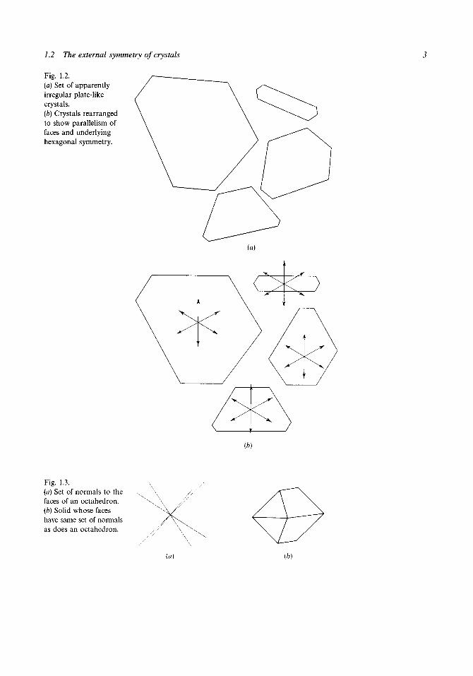
have the same general habit a detailed examination reveals considerablevariation in size and shape. In particular one may find a selection of platycrystals looking somewhat like those shown in fig. 1.2(a). The shapes ofthese seem to be quite unrelated but, if they are rearranged as in fig. 1.2(b), arather striking relationship may be noted. Although the relative sizes of thesides of the crystal cross-sections are very different the normals to the sides(in the plane of the figure) form an identical set from crystal to crystal.Furthermore the set of normals is just that which would be obtained from aregular hexagonal cross-section although none of the crystals in fig. 1.2displays the characteristics of a regular polygon. While this illustration isessentially two-dimensional the same general observations can be made inthree dimensions. Although the crystals of a given species vary greatly in theshapes and sizes of corresponding faces, and may appear to lack symmetryaltogether, the set of normals to the faces will be identical from crystal tocrystal (although a crystal may occasionally lack a particular face completely)and will usually show symmetry that the crystals themselves lack. Forexample, fig. 1.3(a) shows the set of normals for an octahedron. Thesenormals are drawn radiating from a single point and are of equal length.This set may well have been derived from a solid such as that shown in fig.13(b) but the symmetry of the normals reveals that this solid has faceswhose relative orientations have the same relationship as those of theoctahedron.
The presentation of a three-dimensional distribution of normals as donein fig. 1.3 makes difficulties both for the illustrator and also for the viewer.The normals have a common origin and are of equal length so that theirtermini lie on the surface of a sphere. It is possible to represent a sphericaldistribution of points by a perspective projection on to a plane and thestereographic projection is the one most commonly used by the crystallog-rapher. The projection procedure can be followed in fig. 1 A(a). Points on thesurface of the sphere are projected on to a diametral plane with projectionpoint either 0 or O\ where 00' is the diameter normal to the projectionplane. Each point is projected from whichever of O or O' is on the oppositeside of the plane and in this way all the projected points are containedwithin the diametral circle. The projected points may be conventionallyrepresented as above or below the projection plane by full or open circles.Thus the points A, B, C and D project as A\ B\ C and D' and, when viewedalong 00', the projection plane appears as in fig. lA(b).
1.2 The external symmetry of crystals
Fig. 1.2.(a) Set of apparentlyirregular plate-likecrystals.(b) Crystals rearrangedto show parallelism offaces and underlyinghexagonal symmetry.
(b)
Fig. 1.3.(a) Set of normals to thefaces of an octahedron.(b) Solid whose faceshave same set of normalsas does an octahedron.
(a) (b)

The geometry of the crystalline state
Fig. 1.4.(a) The stereographicprojection of pointsfrom the surface of asphere on to adiametral plane.(b) The finalstereographicprojection.
(b)
We now consider the symmetry elements which may be present incrystals - or are revealed as intrinsically present by the set of normals to thefaces.
Centre of symmetry (for symbol see section below entitled 'Inversionaxes')
A crystal has a centre of symmetry if, for a point within it, faces occur inparallel pairs of equal dimensions on opposite sides of the point andequidistant from it. A selection of centrosymmetric crystals is shown in fig.1.5(a). However even when the crystal itself does not have a centre ofsymmetry the intrinsic presence of a centre is shown when normals occur in

1.2 The external symmetry of crystals
collinear pairs. The way in which this shows up on a stereographic pro-jection is illustrated in fig. 1.5(b).
Fig. 1.5.(a) A selection ofcentrosymmetriccrystals.(b) The stereographicprojection of a pair ofcentrosymmetricallyrelated faces.
Mirror plane (written symbol m; graphical symbol —)
This is a plane in the crystal such that the halves on opposide sides of theplane are mirror images of each other. Some crystal forms possessingmirror planes are shown in fig. 1.6(a). Mirror planes show up clearly in astereographic projection when the projecting plane is either parallel to orperpendicular to the mirror plane. The stereographic projections for each ofthe cases is shown in fig. 1.6(b).
(b)
Fig. 1.6.(a) Crystals with mirrorplanes.(b) The stereographicprojections of a pair offaces related by a mirrorplane when the mirrorplane is (i) in the planeof projection; (ii)perpendicular to theplane of projection.

The geometry of the crystalline state
Rotation axes (written symbols 2, 3, 4, 6; graphical symbols
An H-fold rotation axis is one for which rotation through 2n/n leaves theappearance of the crystal unchanged. The values of n which may occur(apart from the trivial case n = 1) are 2, 3,4 and 6 and examples of twofold(diad), threefold (triad), fourfold (tetrad) and sixfold (hexad) axes areillustrated in fig. 1.7 together with the stereographic projections on planesperpendicular to the symmetry axes.
Fig. 1.7.(a) Perspective viewsand views down theaxis for crystalspossessing diad, triad,tetrad and hexad axes.(b) The correspondingstereographicprojections.
Inversion axes (written symbols 1, 2, 3, 4, 6; graphical symbolso, none, A , <f>, $ )
The inversion axes relate crystal planes by a combination of rotation andinversion through a centre. The operation of a 4 axis may be followed in fig.1.8(<z). The face A is first rotated about the axis by n/2 to position A' andthen inverted through O to B. Starting with B, a similar operation gives Cwhich in its turn gives D. The stereographic projections showing thesymmetry of inversion axes are given in fig. 1.8(6); it will be noted that T isidentical to a centre of symmetry and T is the accepted symbol for a centre ofsymmetry. Similarly 2 is identical to m although in this case the symbol m ismore commonly used.
These are all the symmetry elements which may occur in the externalform of the crystal - or be observed in the arrangement of normals evenwhen the crystal itself lacks obvious symmetry.
On the experimental side the determination of a set of normals involvesthe measurement of the various interfacial angles of the crystal. For thispurpose optical goniometers have been designed which use the reflection of

13 The seven crystal systems
Fig. 1.8.(a) A perspective viewof the operation of aninverse tetrad axis.(b) Stereographicprojections for T, 2, 3, 4and 6.
2 =
light from the mirror-like facets of the crystal to define their relativeorientations.
1.3 The seven crystal systems
Even from a limited observation of crystals it would be reasonable tosurmise that the symmetry of the crystal as a whole is somehow connectedwith the symmetry of some smaller subunit within it. If a crystal is fracturedthen the small plane surfaces exposed by the break, no matter in what partof the body of the crystal they originate, show the same angular relationshipsto the faces of the whole crystal and, indeed, are often parallel to the crystalfaces.
The idea of a structural subunit was first advanced in 1784 by Haiiy who

The geometry of the crystalline state
was led to his conclusions by observing the cleavage of calcite. This has athreefold axis of symmetry and by successive cleavage Haiiy extracted fromcalcite crystals small rhomboids of calcite. He argued that the cleavageprocess, if repeated many times, would eventually lead to a small, in-divisible, rhombohedral structural unit and that the triad axis of the crystalas a whole derives from the triad axis of the subunit (see fig. 1.10(fo) fordescription of rhombohedron).
Haiiy's ideas lead to the general consideration of how crystals may bebuilt from small units in the form of parallelepipeds. It is found that,generally the character of the subunits may be inferred from the nature ofthe crystal symmetry. In fig. 1.9 is a cube built up of small cubic subunits; itis true that in this case the subunit could be a rectangular parallelepipedwhich quite accidentally gave a crystal in the shape of a cube. However ifsome other crystal forms which can be built from cubes are examined, forexample the regular octahedron and also the tetrahedron in fig. 1.9, then itis found that the special angles between faces are those corresponding to acubic subunit and to no other.
It is instructive to look at the symmetry of the subunit and the symmetryof the whole crystal. The cube has a centre of symmetry, nine mirror planes,six diad axes, four triad axes and three tetrad axes. All these elements ofsymmetry are shown by the octahedron but the tetrahedron, having sixmirror planes, three inverse tetrad axes and four triad axes, shows lesssymmetry than the cube. Some materials do crystallize as regular tetrahedraand this crystal form implies a cubic subunit. Thus, in some cases, thecrystal as a whole may exhibit less symmetry than its subunit. The commoncharacteristic shown by all crystals having a cubic subunit is the set of four
Fig. 1.9.Various crystal shapeswhich can be built fromcubic subunits:(left) cube;(centre) octahedron;(right) tetrahedron. 1
ii
1.4 The thirty-two crystal classes
triad axes - and conversely all crystals having a set of four triad axes are cubic.Similar considerations lead to the conclusion that there are seven
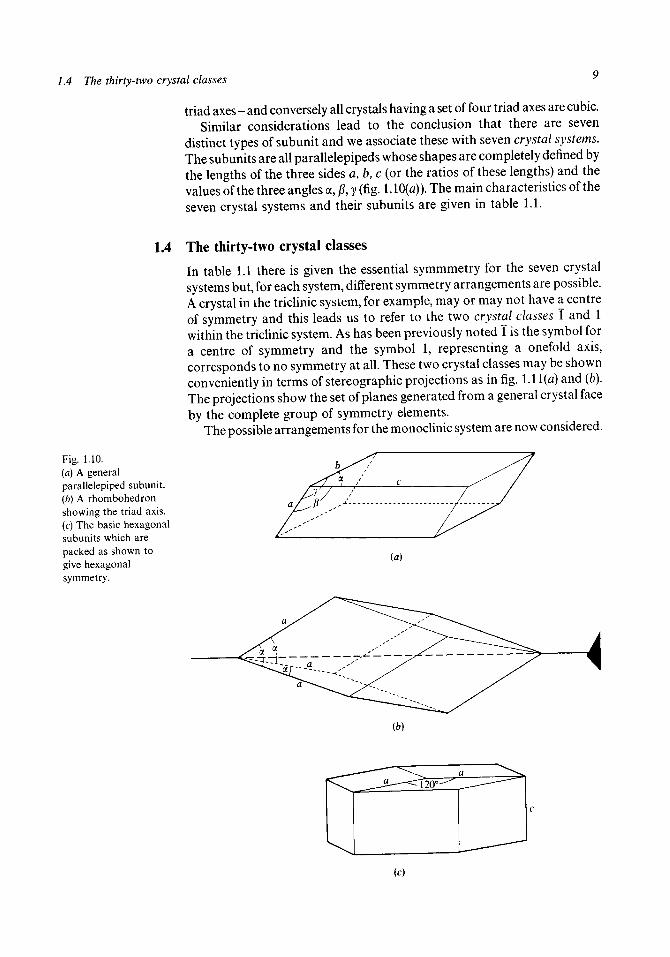
distinct types of subunit and we associate these with seven crystal systems.The subunits are all parallelepipeds whose shapes are completely defined bythe lengths of the three sides a, b, c (or the ratios of these lengths) and thevalues of the three angles a, /?, y (fig. 1.10(a)). The main characteristics of theseven crystal systems and their subunits are given in table 1.1.
1.4 The thirty-two crystal classes
In table 1.1 there is given the essential symmmetry for the seven crystalsystems but, for each system, different symmetry arrangements are possible.A crystal in the triclinic system, for example, may or may not have a centreof symmetry and this leads us to refer to the two crystal classes 1 and 1within the triclinic system. As has been previously noted 1 is the symbol fora centre of symmetry and the symbol 1, representing a onefold axis,corresponds to no symmetry at all. These two crystal classes may be shownconveniently in terms of stereographic projections as in fig. 1.1 \{a) and (b).The projections show the set of planes generated from a general crystal faceby the complete group of symmetry elements.
The possible arrangements for the monoclinic system are now considered.
Fig. 1.10.(a) A generalparallelepiped subunit.(b) A rhombohedronshowing the triad axis.(c) The basic hexagonalsubunits which arepacked as shown togive hexagonalsymmetry.
(a)
(b)
(c)

10 The geometry of the crystalline state
Table 1.1. The seven crystal systems
System
TriclinicMonoclinic
Orthorhombic
Tetragonal
Trigonal
Hexagonal
Cubic
Subunit
No special relationshipsa^b^c0 5* a = 7 = 90°a^b^ca = p = y = 90°a = b 7 c
a = p = y = 90°a = fr = c(X = 0 = y ^ 90°
(see fig. 1.10(6))or as hexagonal
a = b ^ ca = P = 90°, 7 = 120°
(see fig. 1.10(c))a = b = ca = p = y = 90°
Essential symmetry of crystal
NoneDiad axis or mirror plane
(inverse diad axis)Three orthogonal diad or inverse
diad axesOne tetrad or inverse tetrad
axisOne triad or inverse triad
axis
One hexad or inverse hexadaxis
Four triad axes
Fig. 1.11.Stereographicprojections representingthe crystal classes {a) 1and (b) I.
(a) (b)
These, illustrated in fig. 1.12, have (a) a diad axis, (b) a mirror plane and (c) adiad axis and mirror plane together. The orthorhombic and trigonalsystems give rise to the classes shown in fig. 1.13.
Some interesting points may be observed from a study of these diagrams.For example, the combination of symbols 3m implies that the mirror planecontains the triad axis and the trigonal symmetry demands therefore that aset of three mirror planes exists. On the other hand, for the crystal class 3/m,the mirror plane is perpendicular to the triad axis; this class is identical tothe hexagonal class 6 and is usually referred to by the latter name.
It may also be noted that, for the orthorhombic class mm, the symmetryassociated with the third axis need not be stated. This omission is per-missible due to the fact that the two orthogonal mirror planes automaticallygenerate a diad axis along the line of their intersection and a name such as2mm therefore contains redundant information. An alternative name formm is 2m and again the identity of the third symmetry element may be inferred.
For the seven systems together there are thirty-two crystal classes and all

1A The thirty-two crystal classes 11
Fig. 1.12.Stereographic projectionsrepresenting the threecrystal classes in themonoclinic system (a) 2,(b) m and (c) 2/m.
Fig. 1.13.Stereographicprojections representingthe three crystal classesin the orthorhombicsystem and the sixclasses in the trigonalsystem.
32
Trigonal Orthorhombic
crystals may be assigned to one or other of these classes. While the generalnature of the basic subunit determines the crystal system, for each systemthere can be different elements of symmetry associated with the crystal. If amaterial, satisfying some minimization-of-potential-energy criterion, crys-tallizes with some element of symmetry, it strongly implies that there issome corresponding symmetry within the subunit itself. The collection ofsymmetry elements which characterizes the crystal class, and which mustalso be considered to be associated with the basic subunit, is called a pointgroup. It will be seen later that the point group is a macroscopic

12 The geometry of the crystalline state
manifestation of the symmetry with which atoms arrange themselves withinthe subunits.
1.5 The unit cell
We shall now turn our attention to the composition of the structuralsubunits of crystals. The parallelepiped-shaped volume which, when re-produced by close packing in three dimensions, gives the whole crystal iscalled the unit cell. It is well to note that the unit cell may not be an entitywhich can be uniquely defined. In fig. 1.14 there is a two-dimensionalpattern which can be thought of as a portion of the arrangement of atomswithin a crystal. Several possible choices of shape and origin of unit cellare shown and they are all perfectly acceptable in that reproducing theunit cells in a close-packed two-dimensional array gives the correctatomic arrangement. However in this case there is one rectangular unitcell and this choice of unit cell conveys more readily the special rectangularrepeat features of the overall pattern and also shows the mirror plane ofsymmetry. Similar arguments apply in three dimensions in that manydifferent triclinic unit cells can be chosen to represent the structural
Fig. 1.14.A two-dimensionalpattern and somepossible choices of unitcell.

7.5 The unit cell 13
arrangement. One customarily chooses the unit cell which displays thehighest possible symmetry, for this indicates far more clearly the symmetryof the underlying structure.
In §§ 1.3 and 1.4 the ideas were advanced that the symmetry of the crystalwas linked with the symmetry of the unit cell and that the disposition ofcrystal faces depends on the shape of the unit cell. We shall now explore thisidea in a little more detail and it helps, in the first instance, to restrictattention to a two-dimensional model. A crystal made of square unit cells isshown in fig. 1.15. The crystal is apparently irregular in shape but, when theset of normals to the faces is examined we have no doubt that the unit cellhas a tetrad axis of symmetry. The reason why a square unit cell with atetrad axis gives fourfold symmetry in the bulk crystal can also be seen. Ifthe formation of the faces AB and BC is favoured because of the lowpotential energy associated with the atomic arrangement at these boundariesthen CD, DE and the other faces related by tetrad symmetry are alsofavoured because they lead to the same condition at the crystal boundary.
For the two-dimensional crystal in fig. 1.16 the set of normals reveals amirror line of symmetry and from this we know that the unit cell isrectangular. It is required to determine the ratio of the sides of the rectanglefrom measurements of the angles between the faces. The mirror line can belocated (we take the normal to it as the b direction) and the angles made tothis line by the faces can be found. In fig. 1.17 the face AB is formed by pointswhich are separated by la in one direction and b in the other. The angle 0,which the normal AN makes with the b direction, is clearly given by
tan 6 = b/2a. (1.1)
Fig. 1.15.A two-dimensionalcrystal made up of unitcells with a tetrad axis ofsymmetry.

14 The geometry of the crystalline state
Fig. 1.16.A two-dimensionalcrystal built ofrectangular units.
//
\\ \
\
\ \N
\
S.
\\
\\
\
a
\\
\ — /
//
s.
/
\\\
/
\\
••
\
\
Fig. 1.17.The relationship betweenthe crystal face AB andthe unit cell.
/
B
\ /
a
/
If the neighbouring points of the face were separated by na and mb then onewould have
mbtan 0 = —
or
- = - t a n 0 .a m
(1.2)
The angles 0 for the crystal in fig. 1.16 are 32° 12r, 43° 24' and 51° 33' so thatwe have
* = 0 . 6 3 0 ^ = 0.946^. = 1.260^-. (1.3)

1.6 Miller indices 15
We now look for the simplest sets of integers n and m which will satisfyequation (1.3) and these are found to give
- = 0.630 x ? = 0.946 x \ = 1.260 x \.a 1 3 1
From this we deduce the ratio b:a = 1.260:1.This example is only illustrative and it is intended to demonstrate how
measurements on the bulk crystal can give precise information about thesubstructure. For a real crystal, where one is dealing with a three-dimensionalproblem, the task of deducing axial ratios can be far more complicated.
Another type of two-dimensional crystal is one based on a generaloblique cell as illustrated in fig. 1.18. The crystal symmetry shown here is adiad axis (although not essential for this system) and one must deduce fromthe interfacial angles not only the axial ratio but also the interaxial angle.Many choices of unit cell are possible for the oblique system.
The only unconsidered type of two-dimensional crystal is that based on ahexagonal cell where the interaxial angle and axial ratio are fixed.
All the above ideas can be carried over into three dimensions. Gonio-metric measurements enable one to determine the crystal systems, crystalclass, axial ratios and interaxial angles.
1.6 Miller indices
In fig. 1.19 is shown the development of two faces AB and CD of atwo-dimensional crystal. Face AB is generated by steps of 2a, b and CD bysteps of 3a, 2b. Now it is possible to draw lines parallel to the faces such thattheir intercepts on the unit-cell edges are a/h, b/k where h and k are two integers.
The line AB' parallel to AB, for example, has intercepts OA' and OB' ofthe form a/1 and b/2; similarly CD' parallel to CD has intercepts a/2 andft/3. The integers h and k may be chosen in other ways - the line with
Fig. 1.18.A two-dimensionalcrystal based on anoblique unit cell. / / /
/ / // /
/ / // / /
/ / // y
/ / // A 7/ A /
/ /
/ / /\ / /
/ / // // /
/ / // y/ /
/ y• • ' / /
/ /
/ /
/ / /
/ /
/ /
/ /
/
/
/
/
/
/
/
/
/
/
/
/
/ \
\
\
A~7 \y \
A
^ A/ \/ A

16 The geometry of the crystalline state
Fig. 1.19.The lines A'B' and CD'which are parallel to thecrystal faces AB and CDhave intercepts on theunit-cell edges of theform a/h and b/k whereh and k are integers.
intercepts a/2 and b/4 is also parallel to AB. However, we are hereconcerned with the smallest possible integers and these are referred to as theMiller indices of the face.
In three dimensions a plane may always be found, parallel to a crystalface, which makes intercepts a/h, b/k and c/l on the unit-cell edges. Thecrystal face in fig. 1.20 is based on the unit cell shown with OA = 3a,OB = 4b and OC = 2c. The plane A'B'C is parallel to ABC and hasintercepts OA\ OB' and OC given by a/4, b/3 and c/6 (note that thecondition for parallel planes OA/OA' = OB/OB' = OC/OC is satisfied).This face may be referred to by its Miller indices and ABC is the face (436).
The Miller indices are related to a particular unit cell and are thereforenot uniquely defined for a given crystal face. Returning to our two-dimensionalexample, the unit cell in fig. 1.21 is an alternative to that shown in fig. 1.19.The face AB which was the (1,2) face for the cell in fig. 1.19 is the (1,1) facefor the cell in fig. 1.21. However, no matter which unit cell is chosen, one canfind a triplet of integers (generally small) to represent the Miller indices ofthe face.
1.7 Space lattices
In figs. 1.19 and 1.21 are shown alternative choices of unit cell for atwo-dimensional repeated pattern. The two unit cells are quite different inappearance but when they are packed in two-dimensional arrays they eachproduce the same spatial distribution. If one point is chosen to represent theunit cell - the top left-hand corner, the centre or any other defined point -then the array of cells is represented by a lattice of points and theappearance of this lattice does not depend on the choice of unit cell. Oneproperty of this lattice is that if it is placed over the structural pattern theneach point is in an exactly similar environment. This is illustrated in fig. 1.22where the lattice corresponding to figs. 1.19 and 1.21 is placed over thetwo-dimensional pattern and it can be seen that, no matter how the lattice isdisplaced parallel to itself, each of the lattice points will have a similarenvironment.
If we have any repeated pattern in space, such as the distribution ofatoms in a crystal, we can relate to it a space lattice of points which definescompletely the repetition characteristics without reference to the details ofthe repeated motif. In three dimensions there are fourteen distinctive space

1.7 Space lattices 17
Fig. 1.20.The plane A'B'C isparallel to the crystalface ABC and makesintercepts on the celledges of the form a/h,b/k and c/l where h, kand / are integers.
Fig. 1.21.An alternative unit cellto that shown in fig.1.19. The faces AB andCD now have differentMiller indices.
Fig. 1.22.The lattice (small darkcircles) represents thetranslational repeatnature of the patternshown.
• *
lattices known as Bravais lattices. The unit of each lattice is illustrated in fig.1.23; lines connect the points to clarify the relationships between them.Firstly there are seven simple lattices based on the unit-cell shapesappropriate to the seven crystal systems. Six of these are indicated by thesymbol P which means 'primitive', i.e. there is one point associated witheach unit cell of the structure; the primitive rhombohedral lattice is usuallydenoted by R. But other space lattices can also occur. Consider the spacelattice corresponding to the two-dimensional pattern given in fig. 1.24. Thiscould be considered a primitive lattice corresponding to the unit cell showndashed in outline but such a choice would obscure the rectangular repeatrelationship in the pattern. It is appropriate in this case to take the unit cellas the full line rectangle and to say that the cell is centred so that pointsseparated by \at\b are similar. Such a lattice is non-primitive. The threepossible types of non-primitive lattice are:

18 The geometry of the crystalline state
Fig. 1.23.The fourteen Bravaislattices. Theaccompanying diagramsshow the environment ofeach of the lattice points. Monoclinic
P
MonoclinicC
OrthorhombicP
OrthorhombicC
Orthorhombic/
OrthorhombicF
(1st Part)

1.7 Space lattices
Fig. 1.23. (cont)
19
Fig. 1.23. (2nd Part)

20 The geometry of the crystalline state
Fig. 1.24.Two-dimensionl patternshowing two choices ofunit cell - generaloblique (dashed outline)and centred rectangular(full outline).
C-face centring - in which there is a translation vector \a, \b in the Cfaces of the basic unit of the space lattice. A and B-face centringmay also occur;
F-face centring- equivalent to simultaneous A, B and C-face centring; and/-centring - where there is a translation vector \a, \b, \c giving a point at
the intersection of the body diagonals of the basic unit of the spacelattice.
The seven non-primitive space lattices are displayed in fig. 1.23. Any spacelattice corresponds to one or other of the fourteen shown and no otherdistinct space lattices can occur. For each of the lattices, primitive andnon-primitive, the constituent points have similar environments. A fewminutes' study of the figures will confirm the truth of the last statement.
1.8 Symmetry elements
We have noted that there are seven crystal systems each related to the typeof unit cell of the underlying structure. In addition there are thirty-twocrystal classes so that there are differing degrees of symmetry of crystals allbelonging to the same system. This is associated with elements of symmetrywithin the unit cell itself and we shall now consider the possibilities for thesesymmetry elements.
The symmetry elements which were previously considered were thosewhich may be displayed by a crystal (§ 1.2) and it was stated that there arethirty-two possible arrangements of symmetry elements or point groups. Acrystal is a single unrepeated object and an arrangement of symmetryelements all associated with one point can represent the relationships of acrystal face to all symmetry-related faces.
The situation is different when we consider the symmetry within the unitcell, for the periodic repeat pattern of the atomic arrangement gives newpossibilities for symmetry elements. A list of symmetry elements which canbe associated with the atomic arrangement in a unit cell is now given.

1.8 Symmetry elements 21
Fig. 1.25.(a) A centrosymmetricunit cell showing thecomplete family of eightdistinct centres ofsymmetry.(b) A unit cell showingmirror planes.(c) A unit cell showingglide planes.(d) A view down atetrad axis of symmetryshowing the othersymmetry axes whicharise.(e) The operation of a2X axis.(/) The operation of 3i
Centre of symmetry (1)
This is a point in the unit cell such that if there is an atom at vector position rthere is an equivalent atom located at — r. The unit cell in fig. 1.25(a) hascentres of symmetry at its corners. Since all the corners are equivalentpoints the pairs of atoms A and A related by the centre of symmetry at O arerepeated at each of the other corners. This gives rise to other centres ofsymmetry which bisect the edges of the cell and lie also at the face and body
.
0
ST.-V &.. i•: r
LLJ*
(M
id)
U'l
A\

22 The geometry of the crystalline state
centres. While these extra points are also centres of symmetry they are notequivalent to those at the corners since they have different environments.
Mirror plane (m)
In fig. 1.25(b) there is shown a unit cell with mirror planes across twoopposite (equivalent) faces. The plane passing through 0 generates thepoints A2 and B2 from Ax and Bv The repeat distance perpendicular to themirror plane gives equivalent points A\, B\, A2 and B'2 and it can be seenthat there arises another mirror plane displaced by \a from the one through O.
Glide planes (a, b, c, n, d)
The centre of symmetry and the mirror plane are symmetry elements whichare observed in the morphology of crystals. Now we are going to consider asymmetry element for which the periodic nature of the pattern plays afundamental role. The glide-plane symmetry element operates by acombination of mirror reflection and a translation.
The description of this symmetry element is simplified by reference to thevectors a, b and c which define the edges of the unit cell. For an a-glide planeperpendicular to the b direction (fig. 1.25(c)) the point A1 is first reflectedthrough the glide plane to Am and then displaced by ^a to the point A2. Itmust be emphasized that Am is merely a construction point and the netresult of the operation is to generate A2 from Av The repeat of the patterngives a point A2 displaced by — b from A2 and we can see that A2 and A x arerelated by another glide plane parallel to the one through O and displacedby b from it. One may similarly have an a-glide plane perpendicular to cand also b- and c-glide planes perpendicular to one of the other directions.An n-glide plane is one which, if perpendicular to c, gives a displacementcomponent ^a + |b.
The diamond glide-plane d is the most complicated symmetry elementand merits a detailed description. For the operation of a d-glide planeperpendicular to b there are required two planes, Px and P2, which areplaced at the levels y = | and y = §, respectively. For each initial point thereare two separate operations generating two new points. The first operationis reflection in P1 followed by a displacement ^c + ^a, and the second areflection in P2 followed by a displacement^ + ^a. If we begin with a point(x, y, z) then the first operation generates a point an equal distance from theplane y = £ on the opposite side with x and z coordinates increased by £, i.e.the point (x + ^ , | — y,z + ^). The second operation, involving the planeP2, similarly generates a point (x — £, f — y, z + {-). These points, and allsubsequent new points, may be subjected to the same operations and it willbe left as an exercise for the reader to confirm that the following set of eightpoints is generated:
x y z | + x l-y i + z4 - 4 - v 4- — v X A- 7 Y 4-4- v 4--I-7
i-y
2 y
l-y

1.9 Space groups 23
These coordinates show that there are two other glide planes at y = fand y = | associated with displacements |c + £a and ^c — ^a, respectively.
Rotation axes (2, 3, 4, 6)
The modes of operation of rotation axes are shown in fig. 1.7; the newfeature which arises for a repeated pattern is the generation of subsidiaryaxes of symmetry other than those put in initially. This may be seen in fig.1.25(d) which shows a projected view of a tetragonal unit cell down thetetrad axis. The point Ax is operated on by the tetrad axis through O to giveA2, A3 and A± and this pattern is repeated about every equivalent tetradaxis. It is clear that Al9 A'2, A^ and A'£ are related by a tetrad axis,non-equivalent to the one through 0, through the centre of the cell. Asystem of diad axes also occurs and is indicated in the figure.
Screw axes (2X; 31? 32; 41? 42? 43; 61? 62, 63, 64, 65)
These symmetry elements, like glide planes, play no part in the macroscopicstructure of crystals since they depend on the existence of a repeat distance.The behaviour of a 2X axis parallel to a is shown in fig. 1.25(e). The point A x
is first rotated by an angle n round the axis and then displaced by a to giveA2. The same operation repeated on A2 gives A\ which is the equivalentpoint to Ax in the next cell. Thus the operation of the symmetry element 2X
is entirely consistent with the repeat nature of the structural pattern.The actions of the symmetry elements 3j and 32 are illustrated in fig.
1.25(/). The point Ax is rotated by 2rc/3 about the axis and then displaced by^a to give A2. Two further operations give A3 and A\, the latter point beingdisplaced by a from Av The difference between 3X and 32 can either beconsidered as due to different directions of rotation or, alternatively, as dueto having the same rotation sense but displacements of ^a and fa,respectively. The two arrangements produced by these symmetry elementsare enantiomorphic (i.e. in mirror-image relationship).
In general, the symmetry element RD along the a direction involves arotation 2n/R followed by a displacement (D/R)a.
Inversion axes (3, 4, 6)
The action of the inversion axis R is to rotate the point about the axis by anangle 2n/R and then invert through a point contained in the axis. Since Tand 2 are equivalent to a centre of symmetry and mirror plane, respectively,they are not included here as inversion axes.
There is given in table 1.2 a list of symmetry elements and the graphicalsymbols used to represent them.
1.9 Space groups
Symmetry elements can be combined in groups and it can be shown that230 distinctive arrangements are possible. Each of these arrangements iscalled a space group and they are all listed and described in volume A of theInternational Tables for Crystallography. Before describing a few of the 230

24 The geometry of the crystalline state
Table 1.2.
Type of symmetry element Written symbol Graphical symbol
Centre of symmetry
Perpendicular In plane ofto paper paper
Mirror plane
Glide planes
Rotation axes
Screw axes
Inversion axes
m
ab
n
2
3
4
6
2,
3
4
6
c
32
4 2 ,4 3
62> 63, 64, 65
—1 —v1 \
glide in plane arrow showsof paper glide direction
glide out ofplane of paper
71
•A•
A-A
• ***-*A
space groups we shall look at two-dimensional space groups (sometimescalled plane groups) which are the possible arrangements of symmetryelements in two dimensions. There are only 17 of these, reflecting thesmaller number of possible systems, lattices and symmetry elements. Thusthere are:
four crystal systems - oblique, rectangular, square and hexagonal;two types of lattice - primitive (p) and centred (c); andsymmetry elements -
rotation axes 2, 3, 4 and 6mirror line mglide line g.

1.9 Space groups 25
We shall now look at four two-dimensional space groups whichillustrate all possible features.
Oblique p2
This is illustrated in fig. 1.26 in the form given in the International Tables.The twofold axis is at the origin of the cell and it will reproduce one of thestructural units, represented by an open circle, in the way shown. Theright-hand diagram shows the symmetry elements; the twofold axis mani-fests itself in two dimensions as a centre of symmetry. It will be seen thatthree other centres of symmetry are generated - at the points (x, y) = (\, 0),(0,^) and ({,\). The four centres of symmetry are all different in that thestructural arrangement is different as seen from each of them.
Fig. 1.26.The two-dimensionalspace group p2 as itappears in InternationalTables for X-rayCrystallography.
No. 2
O
/o
P2\
O
2 Oblique
O I
Origin at 2
Rectangular cm
This rectangular space group is based on a centred cell and has a mirror lineperpendicular to the y axis. In fig. 1.27 the centring of the cell is seen in thatfor each structural unit with coordinate (x, y) there is another at ( + x, \ + y).In addition, the mirror line is shown relating empty open circles to thosewith commas within them. The significance of the comma is that it indicatesa structural unit which is an enantiomorph of the one without a comma.
The right-hand diagram in fig. 1.27 shows the symmetry elements in theunit cell and mirror lines are indicated at y = 0 and y = \. What is also
Fig. 1.27.The two-dimensional ^space group cm as itappears in InternationalTables for X-rayCrystallography.
0O
0O
No. 5
oO
c l m l
OO
ooOrigin on m
m Rectangular

26 The geometry of the crystalline state
apparent, although it was not a part of the description of the two-dimensionalspace group, is the existence of a set of glide lines interleaving the mirrorlines. The operation of a glide line involves reflection in a line followed by atranslation ^a. Because of the reflection part of the operation, the relatedstructural units are enantiomorphs.
Square pAg
This two-dimensional space group is illustrated in fig. 1.28 and shows thefourfold axes, two sets of glide lines at an angle TI/4 to each other and a set ofmirror lines at n/4 to the edges of the cell. Starting with a single structuralunit there are generated seven others; the resultant eight structural units arethe contents of the square cell. Wherever a pair of structural units arerelated by either a mirror line or a glide line the enantiomorphic relationshipis shown by the presence of a comma in one of them.
Fig. 1.28.The two-dimensionalspace group p4g as itappears in InternationalTables for X-rayCrystallography.
S q u a r e 4mm
oo
o
oo
o
o0
oo
oo
o
p4g m
O
O
No. 12
O
O
O
Origin at 4
Hexagonal p6
As the name of this two-dimensional space group suggests it is based on ahexagonal cell, which is a rhombus with an angle 2it/3 between the axes. Ascan be seen in fig. 1.29 the sixfold axis generates six structural units abouteach origin of the cell. A pair of threefold axes within the cell is also
Fig. 1.29.The two-dimensionalspace group p6 as itappears in InternationalTables for X-rayCrystallography.
Hexagonal 6 No. 16
oOrigin at 6
1.9 Space groups 27
generated. The complete arrangement of symmetry elements is shown in theright-hand diagram of fig. 1.29.
Having established some general characteristics of space groups by thestudy of some relatively simple two-dimensional examples we shall nowlook at five three-dimensional space groups where the third dimensionintroduces complications not found in two dimensions.
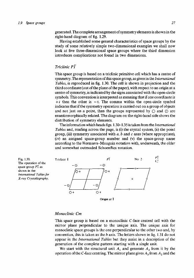
Triclinic PI
This space group is based on a triclinic primitive cell which has a centre ofsymmetry. The representation of this space group, as given in the InternationalTables, is reproduced in fig. 1.30. The cell is shown in projection and thethird coordinate (out of the plane of the paper), with respect to an origin at acentre of symmetry, is indicated by the signs associated with the open-circlesymbols. This convention is interpreted as meaning that if one coordinate is+ £ then the other is —t. The comma within the open-circle symbolindicates that if the symmetry operation is carried out on a group of objectsand not just on a point, then the groups represented by O and 0 areenantiomorphically related. The diagram on the right-hand side shows thedistribution of symmetry elements.
The information which heads figs. 1.30-1.35 is taken from the InternationalTables and, reading across the page, is (i) the crystal system, (ii) the pointgroup, (iii) symmetry associated with a, b and c axes (where appropriate),(iv) an assigned space-group number and (v) the space-group nameaccording to the Hermann-Mauguin notation with, underneath, the olderand somewhat outmoded Schoenflies notation.
Fig. 1.30.The operation of thespace group Pi asshown in theInternational Tables forX-ray Crystallography.
Triclinic 1
/70 +
Monoclinic
0
/
Cm
PI
- 0
1 / o t /
- • / /O +
Origin at T
No. 2
o o
PI
This space group is based on a monoclinic C-face centred cell with themirror plane perpendicular to the unique axis. The unique axis formonoclinic space groups is the one perpendicular to the other two and, byconvention, this is taken as the b axis. The letters shown in fig. 1.31 do notappear in the International Tables but they assist in a description of thegeneration of the complete pattern starting with a single unit.
We start with the structural unit Ax and generate A2 from it by theoperation of the C-face centring. The mirror plane gives A3 from A2 and the

28
Fig. 1.31.The operation of thespace group Cm asshown in theInternational Tables forX-ray Crystallography.The letters have beenadded.
Monoclinic m C 1 m l
The geometry of the crystalline state
No. 8 £ w
+ 0 O + + 0 O +
o +
+ O O + + O O +
Origin on plane m; unique axis b
centring gives 4 4 from A3. This constitutes the entire pattern. The + signsagainst each symbol tell us that the units are all at the same level and thecommas within the open circles indicate the enantiomorphic relationships.
It may be seen that this combination of C-face centring and mirrorplanes produces a set of a-glide planes.
Monoclinic P2Jc
This space group is based on a primitive, monoclinic unit cell with a 2l axisalong b and a oglide plane perpendicular to it. In fig. 1.32(a) these basicsymmetry elements are shown together with the general structural patternproduced by them. It can be found by inspection that other symmetryelements arise; Ax is related to AA and A2 to A3 by glide planes whichinterleave the original set. The pairs of units A4, A2 and Al9 A3 are relatedby a centre of symmetry at a distance \c out of the plane of the paper and awhole set of centres of symmetry may be found which are related as thoseshown in fig. 1.25(a).
The International Tables gives this space group with the unit-cell originat a centre of symmetry and the structure pattern and complete set ofsymmetry elements appears in fig. 1.32(6). If a space group is developedfrom first principles, as has been done here, then the emergence of newsymmetry elements, particularly centres of symmetry, often suggests analternative and preferable choice of origin.
Orthorhombic P212121
This space group is based on a primitive orthorhombic cell and has screwaxes along the three cell-edge directions. The name does not appear todefine completely the disposition of the symmetry elements as it seems thatthere may be a number of ways of arranging the screw axes with respect toeach other.
As was noted in § 1.4 in some point groups certain symmetry elementsappear automatically due to the combination of two others. If this occurs inthe point group it must also be so for any space group based on the pointgroup. If we start with two sets of intersecting screws axes and generate thestructural pattern from first principles we end up with the arrangementshown in fig. 1.33(<z) which corresponds to the space group P21212. Theother possible arrangement, where the original two sets of screw axes do notintersect, is found to give a third set not intersecting the original sets and

1.9 Space groups 29
Fig. 1.32.(a) The developmentfrom first principles ofthe structural patternfor the space groupP2Jc.(b) The description ofP2Jc as given in theInternational Tables forX-ray Crystallography.
. i-oo +
. ii-QO+
o- i-oi+o
(a)
o- i - o
o +
o +
Monoclinic 2/m
- o
P1 2Jc 1
-o0 +
oi- -oO + i + 0
oi- -o
o +
i -
o +
Origin at T; unique axis b
(b)
No. 14 P2JcC5
2b
0 (
Fig. 1.33.(a) The development ofthe structural pattern fortwo sets of 2t axeswhich intersect. Thisgives the space groupK.2,2 .(b) The development ofthe structural pattern forthree sets of 2t axeswhich intersect. Thisgives the space group7222. (From InternationalTables for X-rayCrystallography.)
P 2 x 2 x 2
+ P_
+ O
No. 18 P 2 ,2 ,2 222 Orthorhombic
+ Oo +
-oo-
+ oo +
Orthorhombic 222
+ OO--o
+ o
o+
o-
i+oi - o
o i -oi+
- o
+ o
o +
O +
Origin at 112 in plane of 2 ,2 ,
(a)
7 2 2 2
+ o o -o +
-OO + -OO
Origin at 222
(b)
No. 23 7 2 2 2
—i

30 The geometry of the crystalline state
gives the structural arrangement shown in fig. 1.34 which is the space group
One can have three sets of screw axes in a different arrangement. Forexample, if one starts with three sets of intersecting screw axes one finds thatthree sets of diad axes are also generated and that the unit cell is non-primitive. This space group is the one shown in fig. 1.33(b)-/222.
Fig. 1.34.The space groupP212121 as shown in theInternational Tables forX-ray Crystallography.
Orthorhombic 222
o i -
i + O!
o +
- oi+o
o i -
Origin halfway between three pairs of non-intersecting screw axes
Orthorhombic Aba2
The symbols tell us that there is A-face centring, a fo-glide plane perpendicularto a, an a-glide plane perpendicular to b and a diad axis along c. Thediagrammatic representation of this space group, as given in the InternationalTables, is shown in fig. 1.35. We should notice that the diad axis isautomatically generated by the other two symmetry elements.
Fig. 1.35.The space group Aba!as shown in theInternational Tables forX-ray Crystallography.
Orthorhombic mml
i+oo +
i+o
+ oo +
No.41Abal
+ oo+
+ Q
i+o
© +
+o
t I t If I
Abal
o +
OH
o+ ^ ' *
Origin on 2
The determination of a crystal structure is usually a major undertaking andthe first task of the crystallographer is to determine the space group(chapter 7) and to familiarize himself with its characteristics. Some spacegroups occur frequently, for example P2Jc and P212121 are well known bymost crystallographers; other space groups occur much more rarely andthese would usually be studied, as required, on an ad hoc basis.
1.10 Space group and crystal class
In §1.4 it was illustrated for a two-dimensional square unit cell howsymmetry within the cell influences the way in which cells associate to form

Problems to Chapter 1 31
the complete crystal. The formation of the faces of a crystal in the process ofcrystallization takes place in such a way that the crystal has a configurationof minimum potential energy. If the unit cell contains a diad axis thenclearly, by symmetry, any association of cells giving a particular face will bematched by an associated face related by a crystal diad axis. However ascrew axis in the unit cell will also, in the macroscopic aspect of the wholecrystal, give rise to a crystal diad axis since the external appearance of thecrystal will not be affected by atomic-scale displacements due to a screwaxis. Similarly, mirror planes in the crystal are formed in response to bothmirror planes and glide planes in the unit cell.
In the International Tables the point group is given for each of the listedspace groups. The space groups described in this chapter, with the cor-responding point groups, are:
Space group
P\CmP2JcP212121
Aba!
Point group
rm2/m222mm!
A study of the crystal symmetry can be an important first step in thedetermination of a space group as for a particular point group a limitednumber of associated space groups are possible. However the art ofexamining crystals by optical goniometry is now largely ignored by themodern X-ray crystallographer who tends to use only diffraction informationif possible.
Problems to Chapter 1
1.1 A unit cell has the form of a cube. Find the angles between the normalsto pairs of planes whose Miller indices are:(a) (100) (010); (b) (100) (210); (c) (100) (111); (d) (121) (111).
1.2 The diagrams in fig. 1.36 show a set of equivalent positions in a unit cell.Find the crystal system and suggest a name for the space group.
1.3 Draw diagrams to show a set of equivalent positions and the set ofsymmetry elements for the following space groups:(a) P91 (b) p4mm; (c) Pm; (d) P2/m; (e) 14.
Fig. 1.36.Diagrams for Problem1.2.
o +
o +
+ 0
+ O
o+ Ho
Oi- - 0
o+
0 -
- 0
+o(a) (b) (c)

2 The scattering of X-rays
2.1 A general description of the scattering process
To a greater or lesser extent scattering occurs whenever electromagneticradiation interacts with matter. Perhaps the best-known example is Ray-leigh scattering the results of which are a matter of common everydayobservation. The blue of the sky and the haloes which are seen to surrounddistant lights on a foggy evening are due to the Rayleigh scattering of visiblelight by molecules of gas or particles of dust in the atmosphere.
The type of scattering we are going to consider can be thought of as dueto the absorption of incident radiation with subsequent re-emission. Theabsorbed incident radiation may be in the form of a parallel beam but thescattered radiation is re-emitted in all directions. The spatial distribution ofenergy in the scattered beam depends on the type of scattering processwhich is taking place but there are many general features common to alltypes of scattering.
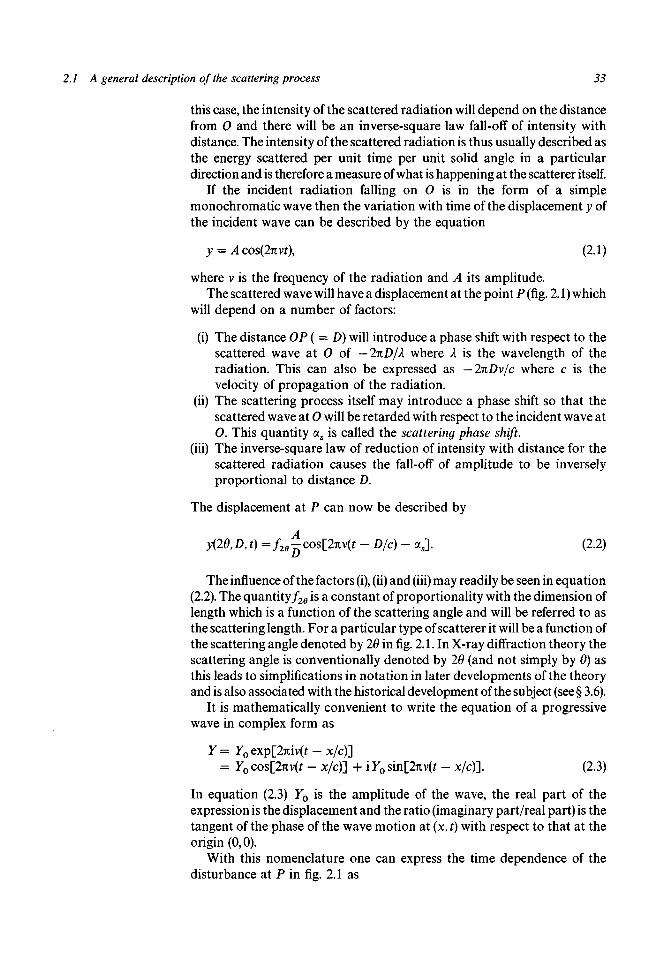
In fig. 2.1 the point O represents a scattering centre. The incidentradiation is in the form of a parallel monochromatic beam and this isrepresented in the figure by the bundle of parallel rays. The intensity at apoint within a beam of radiation is defined as the energy per unit timepassing through unit cross-section perpendicular to the direction ofpropagation of the radiation. Thus for parallel incident radiation theintensity may be described as the power per unit cross-section of the beam.However, the scattered radiation emanates in all directions with somespatial distribution about the point O; this is shown in the figure by drawinga conical bundle of rays with apex at the point O representing the raysscattered within a small solid angle in some particular direction. Clearly, in
Fig. 2.1.Representation of theradiation incident onand scattered from apoint scatterer.
32
2.1 A general description of the scattering process 33
this case, the intensity of the scattered radiation will depend on the distancefrom 0 and there will be an inverse-square law fall-off of intensity withdistance. The intensity of the scattered radiation is thus usually described asthe energy scattered per unit time per unit solid angle in a particulardirection and is therefore a measure of what is happening at the scatterer itself.
If the incident radiation falling on O is in the form of a simplemonochromatic wave then the variation with time of the displacement y ofthe incident wave can be described by the equation
y = A cos(27ivr), (2.1)
where v is the frequency of the radiation and A its amplitude.The scattered wave will have a displacement at the point P (fig. 2.1) which
will depend on a number of factors:
(i) The distance OP ( = D) will introduce a phase shift with respect to thescattered wave at O of —inD/X where X is the wavelength of theradiation. This can also be expressed as —2nDv/c where c is thevelocity of propagation of the radiation.
(ii) The scattering process itself may introduce a phase shift so that thescattered wave at O will be retarded with respect to the incident wave atO. This quantity as is called the scattering phase shift.
(iii) The inverse-square law of reduction of intensity with distance for thescattered radiation causes the fall-off of amplitude to be inverselyproportional to distance D.
The displacement at P can now be described by
y(26,D, t) =f26^cos[_2nv(t - D/c) - a j . (2.2)
The influence of the factors (i), (ii) and (iii) may readily be seen in equation(2.2). The quantity/^ is a constant of proportionality with the dimension oflength which is a function of the scattering angle and will be referred to asthe scattering length. For a particular type of scatterer it will be a function ofthe scattering angle denoted by 28 in fig. 2.1. In X-ray diffraction theory thescattering angle is conventionally denoted by 29 (and not simply by 6) asthis leads to simplifications in notation in later developments of the theoryand is also associated with the historical development of the subject (see§ 3.6).
It is mathematically convenient to write the equation of a progressivewave in complex form as
7=roexp[27iiv(r-x/c)]= Yo cos[27iv(r - x/c)] + i Yo sin[27tv(r - x/c)]. (2.3)
In equation (2.3) Yo is the amplitude of the wave, the real part of theexpression is the displacement and the ratio (imaginary part/real part) is thetangent of the phase of the wave motion at (x, t) with respect to that at theorigin (0,0).
With this nomenclature one can express the time dependence of thedisturbance at P in fig. 2.1 as

34
y{26D, t) =/29^exp[27iiv(t - D/c) - i a j .
The scattering of X-rays
(2.4)
The amplitude of the disturbance at P due to a single scatterer is then given by
t!(2d,D)=f2e^ (2.5)
and the phase lag of the disturbance at P behind the incident wave at 0 is
aOP = 2nvD/c + as. (2.6)
The intensity of the scattered beam in terms of power per unit solid angleis given by
J2e = ]2 x D2 =f2dKA2
or
where K is the constant relating intensity to (amplitude)2 and / 0 is theintensity of the incident beam on the scatterer. The use of the distinctsymbols to represent the differently defined incident and scattered beamintensities should be noted.
2.2 Scattering from a pair of points
Consider the situation shown in fig. 2.2 where radiation is incident on twoidentical scattering centres Ox and O2. We shall find the resultant at P, apoint at a distance r from Ox which is very large compared to the distanceOlO2. Under this condition the scattered radiation which arrives at P hasbeen scattered from Ot and O2 through effectively the same angle 26. Theplanes defined by (i) Ov O2 and the incident beam direction and (ii) OUO2
and P are indicated in fig. 2.2 to emphasize the three-dimensional nature ofthe phenomenon we are considering.
Since the scatterers are identical the scattering phase shift as will be thesame for each. Hence, for the radiation arriving at P the phase difference ofthe radiation scattered at O2 with respect to that scattered at Ox is
Fig. 2.2.Scattering from a pair ofpoint scatterers.
0 , So
Incident radiation
Scattered radiation

Scattering from a pair of points 35
«Oio2=--^(CO2 + O2D). (2.8)
Two unit vectors §0 and S are now defined which lie, respectively, along thedirections of the incident and scattered beams. If the vector joining O1 to O2
is denoted by r then
CO2 = r-S0, O2D = - r §
and thus, from equation (2.8),
(2.9)
The bracketed quantity in equation (2.9) may be replaced by an equivalentvector
s = ^ (210)
giving
aolo2 = 2nT's- (2-n)
The vector s is highly significant in describing the scattering process anda geometrical interpretation of it is shown in fig. 2.3. The vectors So/X andS/X in the incident and scattered directions have equal magnitudes 1/1. Itcan be seen from simple geometry that s is perpendicular to the bisector ofthe angle between So and S and that its magnitude is given by
s = (2sin0)/A. (2.12)
If the displacement due to the incident radiation at Ox is described byequation (2.1) then the resultant disturbance at P, a distance D from Ol9 willbe given by
y(209D,t) =/2,-{exp[27iiv(r - D/c) - iaj
+ exp[27iiv(t — D/c) — ias + 27iir-s]}
= /2e^exp[2itiv(t - D/c) - iaj[l + exp(2iurs)]. (2.13)
The amplitude of this resultant is
Fig. 2.3.The relationship of s to S()/lSo and S.
S/A

36
Fig. 2.4.(a) A phase-vectordiagram for a pair ofpoint scatterers with onepoint as phase origin.(b) A phase-vectordiagram for a pair ofpoint scatterers with ageneral point as phaseorigin.
The scattering of X-rays
which, using equation (2.5), may be expressed in terms of the amplitude ofscattering from a single unit as
rj2(26,D) = exp(2iurs)]. (2.14)
This equation is interpreted in terms of a phase-vector diagram in fig.2.4(a). The amplitude of the disturbance at P due to scattering at Ox isrepresented by the vector AB and that due to scattering at O2 by the vectorBC. Both these vectors have the same magnitude, rt(29,D), and the anglebetween them equals the difference of phase of the radiation scattered fromO1 and O2, 27irs. The resultant AC has magnitude rj2(29,D) and differs inphase from the radiation scattered at Ox by the angle 0.
However in this description we have given a special role to one of thescatterers, Ol9 with respect to which as origin all phases are quoted. Thephase-vector diagram can be drawn with more generality if one measuresphases with respect to radiation which would be scattered from somearbitrary point 0 if in fact a scatterer was present there. Then, if thepositions of Ox and O2 with respect to O are given by the vectors rx and r2,equation (2.14) appears as
ri2(20,D) = f7(20,D)[exp(27tiiys) 4- exp(27iiiyr)]
and the phase-vector diagram appears as in fig. 2.
(2.15)
2.3 Scattering from a general distribution of point scatterers
Let us now examine the scattering from a system of identical pointscatterers Ov O2,..., On. We are interested in the amplitude of the disturbancein some direction corresponding to a scattering vector s at a distance whichis large compared with the extent of the system of scatterers.
If the position of the scatterer at Om is denoted by its vector displacement
0, D) B
(a)

2.4 Thomson scattering 37
rm from some origin point 0 then, by an extension of the treatment whichled to equation (2.15) we find
(2.16)
That this equation applies to identical scatterers is revealed by the factor7/(20, D) appearing outside the summation. When the scatterers are non-equivalent the scattering amplitude must be written
rjn(2e,D)=
= ^ Z (fie)] exp(27iir/s), (2.17)
where the scattering length for each of the scatterers now appears within thesummation symbol. The phase-vector diagram for non-identical scatterersis shown in fig. 2.5 for the case n = 6. It will be evident that, although werefer to the scatterers as non-equivalent, we have assumed that they all havethe same associated values of as. This is the usual situation with X-raydiffraction. However it is sometimes possible to have the scatterers withdiffering phase shifts and, when this happens, useful information may beobtained (§8.5).
We shall find later that equation (2.17) is the basic equation fordescribing the phenomenon of X-ray diffraction and, when the symmetry ofthe atomic arrangements within crystals is taken into account, that it mayappear in a number of modified forms.
2.4 Thomson scattering
We have discussed the results of scattering by distributions of scattererswithout concerning ourselves with the nature of the scatterers or of thescattering process. It turns out that the scatterers of interest to us areelectrons and the theory of the scattering of electromagnetic waves by free(i.e. unbound and unrestrained) electrons was first given by J. J. Thomson.
Fig. 2.5.A phase-vector diagramfor six non-identicalscatterers.
2nrh • s

38 The scattering of X-rays
The basic mechanism of Thomson scattering is simple to understand.When an electromagnetic wave impinges on an electron the alternatingelectric-field vector imparts to the electron an alternating acceleration, andclassical electromagnetic theory tells us that an accelerating chargedparticle emits electromagnetic waves. Thus the process may be envisaged asthe absorption and re-emission of radiation and, although the incidentradiation is unidirectional, the scattered radiation will be emitted in alldirections. If we have the straightforward case where the incident radiationis a single, continuous and monochromatic wave then the acceleration ofthe electron will undergo a simple harmonic variation and the incident andemitted radiation will quite obviously have the same frequency.
If an electron at 0, of charge e and mass m, is undergoing an oscillationsuch that the acceleration is periodic with amplitude a (fig. 2.6) then theorytells us that the scattered radiation at P, which is travelling in the directionOP, has an electric vector of amplitude
E =ea sin (/>
4nsorc2 (2.18)
which is perpendicular to OP and in the plane defined by OP and a. Here, £0
is the permittivity of free space.In fig. 2.7 a parallel beam of electromagnetic radiation travelling along
OX falls upon an electron at O. We wish to determine the nature of thescattered wave at P. The amplitude of the electric vector E of the incidentwave is perpendicular to OX and may be resolved into components E± and£|l perpendicular to and in the plane OX P. The electron will havecorresponding components of acceleration of amplitudes
Fig. 2.6.The relationship of theelectric vector ofscattered electromagneticradiation at a point P tothe acceleration vector ofan electron at 0. Thevectors are both in theplane of the diagram.
Fig. 2.7.The relationship of thecomponents of theelectric vector ofscattered electromagneticradiation at P to thecomponents of theelectric vector of theincident radiation at 0.
Accelerationvector
Electricvector
Direction of scatter

2.4 Thomson scattering 39
and
Applying equation (2.18) we find the electric vector components of thescattered wave at P as
1 4n£orc2m
and
e2cos 2011 4n£orc2m
The quantity e2/4n£oc2m, which has the dimensions of length and equals
2.82 x 10~15m, is referred to in classical electromagnetic theory as theradius of the electron.
Although we have been thinking about a simple, continuous, monochro-matic, electromagnetic wave all the theory described above can be appliedwhen the incident radiation is complex in form. A complicated incidentwave may be analysed into simple components (see chapter 4) and theresultant electron acceleration and re-radiation may be found by addingtogether the effects of the simple components. Thus E± and E^ may bethought of as the components of the amplitude of any arbitrary electromag-netic radiation arriving at O.
If the intensity of the incident radiation is Io and if this radiation isunpolarized then
= CI0, say. (2.21)
The intensity of the scattered radiation, defined as the power per unit solidangle scattered through an angle 20 is given by
1
Af-^—Yn^^2\4n£oc
2m (1 + cos2 20)10. (2.22)
The factor 1/m2 in equation (2.22) shows why electrons are the onlyeffective scatterers; the lightest nucleus, the proton, has the same magnitudeof charge as the electron but 1837 times the mass.
Thomson scattering is coherent, that is to say there is a definite phaserelationship between the incident and scattered radiation; in the case of afree electron the scattering phase shift is n. In all the processes concernedwith the scattering of X-rays the electrons are bound into atoms and in § 2.6we shall investigate the form of the scattering from the total assemblage ofelectrons contained in an atom.

40 The scattering of X-rays
It is instructive to determine the proportion of the power of a beamincident on a material which will be scattered. First we calculate the totalpower scattered for each individual electron. In fig. 2.8 the point Orepresents the electron and OX the direction of the incident beam. Thepower d^J scattered into the solid angle dft, defined by the region betweenthe surfaces of the cones of semi-angles y and y + dy, is
and since dQ = 27tsinydy and <fy is given by equation (2.22) we have
e2 -(1 + cos2 y)I0 sin y dy.
\4ne0c2mj
Hence the total power scattered by a single electron is
(1 + cos2y)sinydy
(2.23)
\4%soc2m } °
_ 8 T C / - 2 X 2(3 \4%eoc
2m °' (2.24)
For a material containing n electrons per unit volume immersed in aparallel incident beam of cross-sectional area /? the power of the incidentbeam is jS/0 (since 70, the intensity, is the power per unit area of the incidentbeam). The number of electrons traversed by the beam per unit length ofpath is n/i and hence the total power scattered per unit path is, by equation(2.24),
3 \4ii£oc m Pnlo- (2.25)
The ratio of % to the power in the incident beam, /?/0, is called the scatteringpower of the material and is
Fig. 2.8.The solid angle betweenthe surfaces of thecoaxial cones ofsemi-angles y and y + dyis the area of the annularregion on the surface ofthe unit sphere.

2.4 Thomson scattering 41
c = —— =3 \4nsoc
2m n. (2.26)
The quantity o is the fraction of the incident radiation scattered per unitlength of path (one metre in SI units).
If it is assumed that all the electrons in a material are free we can make anestimate of the fraction of the incident radiation which is scattered. Forexample a material of specific gravity 1.2 consisting of light atoms (say ofatomic weight less than 30) would contain about 3 x 1029 electrons m~3.This value of n substituted in equation (2.26) gives a — 20. Since the crystalsused in X-ray diffraction usually have dimensions less than 1 mm it will beseen that only 2% or less of the incident X-ray beam is scattered.
However for the scattering which normally occurs when X-rays interactwith matter the electrons are bound with various degrees of strength to thenuclei of atoms. The advent of the laser has made possible the directmeasurement of Thomson scattering by the interaction of light from a rubylaser with an intense electron beam. In an experiment by Fiocco andThompson (1963), illustrated in fig. 2.9, a 75 mA, 2kV electron beam,magnetically focussed to give an electron density within the beam of5 x 1015 m~3 was crossed by a beam from a ruby laser. This laser gave aburst of 20 joules of light in about 800 fxs and the light measured by thephotomultiplier detector had an intensity about 10 ~ 8 of that of the incidentbeam. The scattered light was of two types - some was scattered by theelectron beam and there was also stray light reflected from the walls of theapparatus. The central feature of this experiment was that it was possible toseparate the stray light from the Thomson-scattered component. Since thescattering was from rapidly moving electrons (speed about one-tenth ofthat of light) there was a Doppler shift in frequency. This shift was about260 A and with a suitable filter the stray radiation, whose wavelength wasunshifted, could be prevented from reaching the detector.
This experiment barely detected the presence of Thomson scattering asthere were very few (less than ten) scattered photons per pulse. Later workusing higher-current electron beams and more powerful lasers has enableda direct confirmation of equation (2.22) to be made (see Problem 2.3 at theend of this chapter).
Fig. 2.9.The arrangement ofcomponents of theFiocco and Thompson(1963) experiment.
Collector forun scatteredradiation

42 The scattering of X-rays
2.5 Compton scattering
Experimentally it is found that the radiation scattered by materials consistsof two parts. The first part, that associated with Thomson scattering, hasthe same wavelength as the incident radiation; the second part has awavelength longer than that of the incident radiation with the difference ofwavelength depending on the angle of scatter. This latter component is dueto what is known as Compton scattering and it is incoherent with theincident radiation. It is best described in terms of the elastic collision of aphoton with an electron. In fig. 2.10(a) the incident photon moves along thedirection PO and, after collision with the electron, moves off along OQ whilethe electron recoils along OR. From the conservation of energy in the elasticcollision we find that
he he 1 2
T ~ X + dX + 2™V
or, making usual approximations,
heT2' (2.27)
In addition to energy, momentum must also be conserved and in fig.2.10(fr) is shown the appropriate momentum vector diagram. It is a validapproximation to ignore the change in magnitude of the momentum of thescattered photon and thus we deduce from simple geometry that
±mv = - sin 6.A
(2.28)
Fig. 2.10.(a) Velocity vectordiagram for Comptonscattering of a photon byan electron.(b) Momentum vectordiagram for Comptonscattering.
Scattered photonhe
energy =
Incident photonhe
energy = —\
Recoil electronenergy = jmv2
(a)
Scattered photon _ J7
momentum magnitude 6
Recoil electronmomentum magnitude = mv
Incident photonmomentum magnitude = hjX
(b)
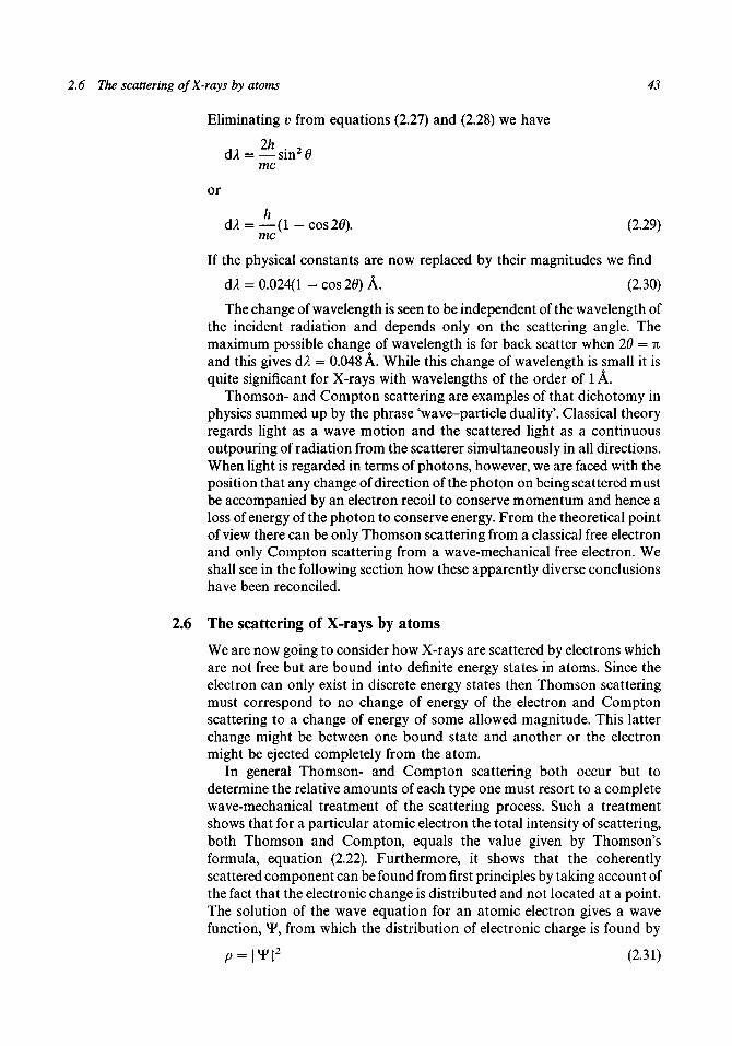
2.6 The scattering of X-rays by atoms 43
Eliminating v from equations (2.27) and (2.28) we have
<U = — sin20me
or
dX = — (1 -cos 20). (2.29)
If the physical constants are now replaced by their magnitudes we find
(U = 0.024(1 - cos 20) A. (2.30)
The change of wavelength is seen to be independent of the wavelength ofthe incident radiation and depends only on the scattering angle. Themaximum possible change of wavelength is for back scatter when 26 = %and this gives dk = 0.048 A. While this change of wavelength is small it isquite significant for X-rays with wavelengths of the order of 1 A.
Thomson- and Compton scattering are examples of that dichotomy inphysics summed up by the phrase 'wave-particle duality'. Classical theoryregards light as a wave motion and the scattered light as a continuousoutpouring of radiation from the scatterer simultaneously in all directions.When light is regarded in terms of photons, however, we are faced with theposition that any change of direction of the photon on being scattered mustbe accompanied by an electron recoil to conserve momentum and hence aloss of energy of the photon to conserve energy. From the theoretical pointof view there can be only Thomson scattering from a classical free electronand only Compton scattering from a wave-mechanical free electron. Weshall see in the following section how these apparently diverse conclusionshave been reconciled.
2.6 The scattering of X-rays by atoms
We are now going to consider how X-rays are scattered by electrons whichare not free but are bound into definite energy states in atoms. Since theelectron can only exist in discrete energy states then Thomson scatteringmust correspond to no change of energy of the electron and Comptonscattering to a change of energy of some allowed magnitude. This latterchange might be between one bound state and another or the electronmight be ejected completely from the atom.
In general Thomson- and Compton scattering both occur but todetermine the relative amounts of each type one must resort to a completewave-mechanical treatment of the scattering process. Such a treatmentshows that for a particular atomic electron the total intensity of scattering,both Thomson and Compton, equals the value given by Thomson'sformula, equation (2.22). Furthermore, it shows that the coherentlyscattered component can be found from first principles by taking account ofthe fact that the electronic change is distributed and not located at a point.The solution of the wave equation for an atomic electron gives a wavefunction, x¥, from which the distribution of electronic charge is found by
p = \V\2 (2.31)
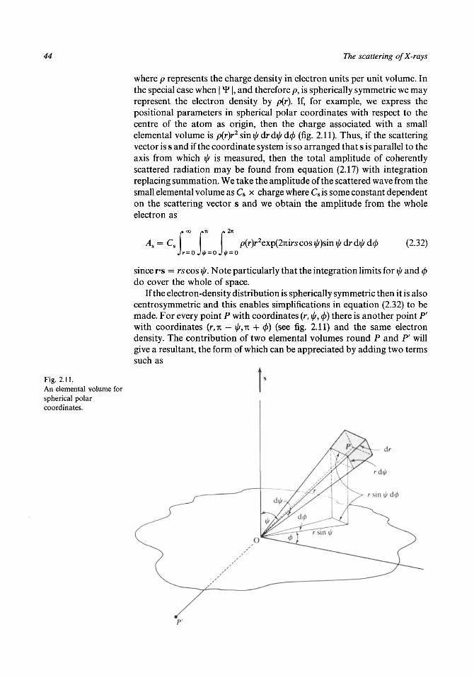
44 The scattering of X-rays
Fig. 2.11.An elemental volume forspherical polarcoordinates.
where p represents the charge density in electron units per unit volume. Inthe special case when | *F |, and therefore p, is spherically symmetric we mayrepresent the electron density by p(r). If, for example, we express thepositional parameters in spherical polar coordinates with respect to thecentre of the atom as origin, then the charge associated with a smallelemental volume is p{r)r2 sin ij/dr dij/d(/> (fig. 2.11). Thus, if the scatteringvector is s and if the coordinate system is so arranged that s is parallel to theaxis from which i// is measured, then the total amplitude of coherentlyscattered radiation may be found from equation (2.17) with integrationreplacing summation. We take the amplitude of the scattered wave from thesmall elemental volume as Cs x charge where Cs is some constant dependenton the scattering vector s and we obtain the amplitude from the wholeelectron as
As = Cs p(r)r2Qxp(2nirs cos i/f)sin \// dr d ^ dcf)J r = O J\J/ = O J ^ = 0
(2.32)
since r*s = rs cos \jt. Note particularly that the integration limits for \jj and 0do cover the whole of space.
If the electron-density distribution is spherically symmetric then it is alsocentrosymmetric and this enables simplifications in equation (2.32) to bemade. For every point P with coordinates (r, ij/, <f>) there is another point P'with coordinates (r,n — ij/,n + </>) (see fig. 2.11) and the same electrondensity. The contribution of two elemental volumes round P and P' willgive a resultant, the form of which can be appreciated by adding two termssuch as

2.6 The scattering of X-rays by atoms 45
) + exp[27iirs COS(TI — \jj)~]= exp(27iirs cos \j/) + exp( — 2nirs cos \j/)= 2cos(2iirscos^).
It is clear from this that As is a real quantity for a centrosymmetricdistribution of electron density and that equation (2.32) can be rewritten as
As=cA p(r)r2cos(2nrs cos ^)sin x// Ar d\jj d0 (2.33)
The fact that p(r) is independent of \\t and 0 enables one to integrate overthese latter variables giving
For a given value of s we shall now find the scattered amplitude from p(r)as a fraction ps of that amplitude, say (As)o, which would be given by a pointelectron at the origin. This may be found from equation (2.34) by notingthat a point electron at the origin has an electron density p(r) = d(r). Thedelta function d(r) has the property
S(r) = oo, r = 0,
and J <5(r) dt? = 1, where the integration can be over any finite volume ofspace around the origin.
For a delta-function electron density there is no contribution toequation (2.34) away from the origin and since
sin(27i rs)^
2nrs
and, by definition
. 0 0
4TI 5(r)r2dr= 1Jr = O
then it follows that
From this we find
(2.36)
where we recognize that p depends only on the magnitude of s by droppingthe vector notation in the subscript. If an atom contains Z electrons thenthe total electron density, pa(r), will be the sum of the densities of theindividual electrons, i.e.

46 The scattering of X-rays
pJr) = I pfo). (2.37)
The amplitude of coherent scattering from the total electron density willbe obtained by adding the amplitudes for the electrons taken individually.We now define an atomic scattering factor fa as the ratio of the amplitude ofthe coherent scattered radiation from an atom to that from a single electronsituated at the atomic centre. This is derived from equations (2.36) and (2.37)and is
4\^dr=i>s), (2.38)
Atomic scattering factors are well tabulated in vol. Ill of the InternationalTables for X-ray Crystallography. Various models of atoms have been usedto give electron-density distributions. For light atoms the Hartreeself-consistent field method of computing wave functions is usually employed,while for heavy atoms the Thomas-Fermi approximation may be used.
We can now investigate the nature of Compton scattering from atoms.From equation (2.36) we can see that the intensity of coherent scatteringfrom an atomic electron is p\^ 2Q and hence, since the total intensity ofscattering as revealed by wave mechanics is J2By the intensity of theCompton scattering must be (1 — Ps)^2o- However the Compton scatteringfrom one atomic electron is incoherent with respect to that scattered by anyother and hence the total intensity from all the electrons is obtained byadding the individual intensities from each of the electrons. Thus we have
^Comp,on = Z{1-(PS),?}X^2«> (2.39)j= 1
and
j i ] 22 ( , (2.40)
It will be seen from equation (2.36) that since for s = 0 (9 = 0) we have
/sin(27irs)\
V 2 )
then p0 = 1. Hence, for radiation scattered in the incident-beam directionthere is no incoherent component. As 6 increases so p decreases but the rateof decrease is less for those electrons which are most tightly bound in theatom. In fig. 2.12(a) there are given the radial electron-density distributions,4nr2p(r), for the six electrons of the carbon atom calculated from Slater'sapproximate analytic wave functions. In fact there are two Is electrons, two2s electrons and two 2p electrons; when radial symmetry is assumed (andthis is an assumption which, although usually made, is not really justifiedfor 2p electrons) the 2s and 2p electrons give equivalent radial electron-densitydistributions.

2.6 The scattering of X-rays by atoms 47
Fig. 2.12.(a) The radialelectron-density functionsof Is and 2s electrons ofa carbon atom asdefined by Slater'sanalytic wave functions.(b) The amplitude ofscattering from the Isand 2s electrons.(c) The atomic scatteringfactor/a for the carbonatom and the coherentand incoherent scatteredintensities from a singleatom.
4nr2p(r)
1.0r
(a)
2.0
1.0
0.5
Is
2.0

48 The scattering of X-rays
From the Slater formulae we find
c3
pls(r) = — exp( — 2cxr) (2.41)
and
(2.42)
where, for carbon, c1 = 10.77 A " 1 and c2 = 6.15 A" 1 .The much tighter distribution of the Is electrons can be appreciated from
fig. 2.12(a). For a given value of s(9) if more of the electronic charge isconcentrated at low values of r then more of the contribution of theintegration, equation (2.36), is for regions of space where sin(2nrs)/2nrs isclose to unity and hence ps will also be closer to unity.
For the analytical expressions (2.41) and (2.42) we find from equation (2.36)
and
A *\ I 0 / f\ \ ***M
-M
-M
-\**•v* * •* / « 1 / / • % A ^ \
Zx/* I I* PYHI /P VI (\Y r=z - l / dil— 'TC i I / CAUI Z.C i / I "" U7 — " x ^ TTT \ ^ « " * ^ /
Jr = O
C2VC2 ~~ 4 7 1 S )yFsns (4 + 4u V ) 4 '
In fig. 2.12(fe) there are plotted the values of (ps)ls and (ps)2s and it can beseen how the tighter distribution of electron density for the Is electron leadsto a slower fall-off in the value of ps.
The total coherent scattering amplitude/a is found by adding togetherthe values of ps for the individual electrons and this is shown in fig. 2.12(c)together with^f the total coherent scattered intensity from a single atom.The incoherent scattered intensity is found from equation (2.39) and is alsoshown plotted in fig. 2.12(c); it appears that for a single atom the incoherentscattering is quite appreciable for high values of s. However under theconditions of the diffraction of X-rays from crystals, very large numbers ofatoms co-operatively scatter so that the amplitudes of the coherentscattering from different atoms add together whereas for the incoherentscattering it is the intensities which add. Thus when we consider thediffraction of X-rays by crystals incoherent scattering may generally beignored.
Problems to Chapter 2
2.1 Four identical coherent scatterers are placed in a row with a distance 31between neighbours. Radiation of wavelength X falls on the scatterersalong a direction which is normal to the row.
(a) For scattering angles 26 = 0 to 180°, in steps of 20°, determine thescattered amplitudes and intensities as fractions of that whichwould result if all four scatterers were at one point. Plot the results.

Problems to Chapter 2 49
(b) For the same values of 20 find the phases of the resultant scatteredradiation with respect to that from a scatterer at one end of the line.
2.2 Eight identical coherent scatterers are placed at the corners of a cube ofside L A parallel beam of radiation of wavelength A, moving along thedirection of a body diagonal of the cube, falls on the scatterers. What isthe ratio of the intensity of the scattering along the direction of one ofthe sides of the cube compared to that which would be obtained from asingle scatterer for the same scattering angle?(Note: there are two directions to be considered, one representingforward and the other backward scatter.)
2.3 In an experiment to investigate scattering from free electrons afield-emission discharge of 2 kV electrons of 5000 A is confined within acylinder of 4 mm diameter. A Q-spoiled ruby laser produces a 10 joulepulse of duration shorter than that of the field emission and this passesin a fine pencil through the centre of, and perpendicular to, the electronbeam. A detector is arranged to collect the light scattered through anangle of 45° from a solid angle of 0.01 steradian. Calculate, approximately,the number of photons entering the detector.
2.4 A lithium atom contains two Is and one 2s electrons for which theSlater analytic wave functions are
and
x//2s = (ci/96n)*rexp( - \c2r)
where
cl = 5.10A"1 and c2 = 2.46A"1.
Show graphically the radial electron densities for a Is and 2s electronand the amplitude of the coherent scattering from each of them. Plotalso the intensity of (a) the coherent; and (b) the incoherent scatteringfrom a single Li atom.(Note: to calculate points for plotting the curves the recommendedintervals are -
pls: r = 0-1.0 A by steps of 0.1 A;p2s: r = 0-2.0 A by steps of 0.2 A;
and
p:s = 0-2.0A"1 by steps of 0.2A"1.)

3 Diffraction from a crystal
3.1 Diffraction from a one-dimensional array of atoms
A crystal consists of a three-dimensional periodic arrangement of atomseach of which will scatter an incident X-ray beam. The scattered radiationfrom each of the atoms is coherent with respect to that from all others andwe have seen in § 2.3 how to compute the resultant scattered amplitude. Weare now going to examine in detail the influence of the periodic nature of theatomic arrangement in the diffraction of X-rays by a crystal. It is useful firstof all to consider diffraction from a single row of n atoms, each atomseparated from its neighbour by a vector distance a.
Previously, in the reasoning which led to equation (2.33), it was foundthat the scattering amplitude from a centrosymmetric arrangement ofscatterers is real if the centre of symmetry is used as origin. The analysis ofthe present case is simplified if we assume that n is odd and if we take thecentre atom, which is at the centre of symmetry, as the coordinate origin.
In a direction corresponding to a scattering vector s, and at somedistance which is large compared with the extent of the lattice, theamplitude of the scattered radiation, expressed as a fraction of that from apoint electron at the origin, is
4 . = / . I cos(27i<za-s), (3.1)
where/a is the atomic scattering factor.This expression can be simplified as follows:
a {sin(7irca*s) — sin[7i(n — 2)a#s]2 sin(7ta*s)
+ sin[7i(n — 2)a's] — sin[7t(w — 4)a*s]
+ • • • + sin[7t(2 — n)a*s] — sin[7t( — n)a*s]}.
The terms on the right-hand side all cancel except the first and last, whichare equal, and we have
sin(7ina-s)
This equation can be found to hold also for n even, if the centre ofsymmetry is used as origin, and equation (3.2) must give the magnitude of

3.1 Diffraction from a one-dimensional array of atoms 51
Fig. 3.1.The functions sin2(5ita*s)and sin2(7ia*s).
the scattered amplitude no matter what origin is chosen. The intensity ofscattering is given by
sin2(7ia#s)=/2(Kn)2,say, (3.3)
and it will be instructive to examine the properties of (Kn)2 as a function of
a#s for various values of n. If we look at (Kn) we see that for a»s = h, where his an integer, both sin(iina*s) and sin(7ia*s) are zero. However, we candetermine the corresponding value of (Kn) by noting that
[sin2(nx)
sin2*M 2 _ n2
=— — n .(3.4)
In fig. 3.1 there are plotted the functions sin2(7ina#s) and sin2(7ia's) for n = 5.It is evident that the ratio of these two functions will be periodic with arepeat distance of unity so that if (Kn)
2 = n2 for a*s = 0 it is also equal to n2
for a#s = h, where h is any positive or negative integer.In fig. 3.2, for the range a*s = 0 to 1 the function (Kn)
2 is showngraphically for n = 3, 5 and 7. The vertical scale of these graphs has beenadjusted to reveal more clearly the relative variation of (Kn)
2 as a*s changes.The following then are the general characteristics of the functions (Kn)
2.
(1) The main maxima of (Kn)2 occur whenever a#s equals an integer.
(2) Between the main maxima there are n — 1 minima, where (Kn)2 is zero,
and n — 2 subsidiary maxima.(3) The width of a main maximum is 2/n and the maxima therefore get
narrower as n increases.(4) The main peak is twice as wide as the subsidiary ones.(5) The ratio of the heights of the main to subsidiary maxima increases as n
increases.
The case n = 4 can be followed in the sequence of phase-vector diagramsshown in fig. 3.3. As a*s progresses from 0 to 1 we can see the development ofthe three minima and two subsidiary maxima. In fact the positions shownas subsidiary maxima in fig. 3.3 are close to but not actually at the maxima.
The maxima of(Kn)2 lie close to the maxima of sin2(7i/ia*s), being closer
sin (Tea • s)0.5 1.0 1.5

52 Diffraction from a crystal
Fig. 3.2.The intensity ofscattering from rows of3, 5 and 7 scatterers asfunctions of a*s.
10
1.0
the larger the value of n and the faster the variation of sin2(7trca-s) comparedto sin2(7ia*s). As n tends to infinity, when the two sets of maxima tend tocoincide, we may write the positions of the maxima of (Kn)
2 as
2m + 1a*s = — , m = 1 to n — 2.
2n
Thus the height of the first subsidiary peak, that for m = 1, is given by
sin2[7i(3/2n)]
and the ratio of height of the first subsidiary peak to the main peak is
= ^ 1 = 0.045. (3.5a)

3.1 Diffraction from a one-dimensional array of atoms 53
Fig. 3.3.Phase-vector diagramshowing the formationof maxima and minimaof intensity for a row offour scatterers.
Main maximuma • s = 0
First minimum
First subsidiary maximuma s — i
A_CE
Second minimum
Second subsidiary maximum
Third minimuma s = 5
A B C D
Similarly for the mth peak, as long as m « n, we find
(Kn)(2m+ l)/2n _ 4
+ Main maximumE as = 1
(Knf0 (2m + 1) V(3.5b)
We may note that this ratio falls oflf rapidly with increasing m and that forlarge n all the subsidiary peaks of appreciable magnitude are very close tothe main maximum. For very large n (theoretically n = oo) we deduce that

54 Diffraction from a crystal
there is no significant diffracted intensity except under the condition
Fig. 3.4.The relationship ofincident and diffractedX-rays to a row ofatoms.
a*s = h (an integer). (3.6)
This condition is the one which will be found to apply in the diffraction ofX-rays by crystals where, in the packing of the unit cells in any onedirection, n is rarely less than several hundred. Where the crystal is verysmall there can be some spreading out of the diffraction pattern and thiseffect is discussed further in §6.1.
There can also be found the condition for diffraction from a one-dimensional array of atoms from a more direct physical point of view. In fig.3.4 radiation is shown falling on the row of atoms, the incident radiationmaking an angle \j/a>0 with the row, and we consider the resultant in adirection making an angle y\ia with the row.
For reinforcement of radiation scattered from neighbouring atoms wemust have
CB - AD = hi
where h is an integer, or
a{cos \\ia - cos \jfat0) = hL (3.7)
It should be particularly noticed that the lines representing the incidentbeam, row of atoms and diffracted beam are not necessarily coplanar andfor a particular angle \jja 0 and integer h the permitted angle \\ia defines acone of semi-angle \jja whose axis is the row of atoms. The various values of hdefine a whole family of cones whose surfaces indicate directions in whichthe diffracted intensity is non-zero. These are represented in fig. 3.5(a) whereone of the cones is illustrated, for h = 3, and the other cones are representedby their circular intersections on the sphere, which is so large that thecomplete array of atoms can be considered as situated at the point O. Forh = 0 we see from equation (3.7) that \j/a = \j/a0 and hence the incident beammust lie on the surface of this cone. As the angle \jja 0 is varied so the circlesshown in fig. 3.5 slide round the sphere, staying always perpendicular to andwith their centres on the line OP. Thus if \\ia 0 is made steadily smaller thecircle h — 3 will shrink and finally disappear while the other circles moveround the sphere towards the point P. New circles will appear at the rear ofthe moving system of circles (h = — 5 , - 6 , etc.) until, finally, when \j/a 0 = 0the situation will appear as in fig. 3.5(fc).

3.1 Diffraction from a one-dimensional array of atoms 55
Fig. 3.5.(a) The allowed cones ofdiffraction from aone-dimensional array ofatoms shown by theirintersections with asphere.(b) The orders ofdiffraction which occurwhen the incident beamis aligned with the rowof atoms.
Incident ray
h= -
(a)
h =
Direct ion ^of arra> and
of incident ray(*)
It should be noted that the two conditions for diffraction to occur,
equations (3.6) and (3.7), are equivalent. From equations (3.6) and (2.10) we
have
(3.8)
Since S and So are unit vectors making angles i//a and \jja0, respectively,

56 Diffraction from a crystal
with a then it is clear that equation (3.7) follows immediately from equation(3.8).
3.2 Diffraction from a two-dimensional array of atoms
We can now progress to the consideration of diffraction from a two-dimensional array of atoms (fig. 3.6) which can be defined in terms of twovectors a and b. The condition that the radiation scattered by all the atomsof the array shall constructively interfere can be broken down into the pairof conditions - (i) that the radiation scattered by the atoms of separation ashall constructively interfere, and (ii) all the radiation scattered by atoms ofseparation b shall constructively interfere. This leads to the pair of equations
a#s = h
and
(3.9)
where h and k are two integers.If the angles made by the incident and diffracted beams with the a and b
directions are \\ia 0, ij/a, \jjb0 and \//b then these conditions can also be written as
(3.10)
and
&(cos^-cos^ftf()) =
The equations (3.10) define two families of conical surfaces with axesalong the a and b directions, respectively. These are represented in fig. 3.7 bythe two families of circles on the surface of the sphere, these being theintersections of the cones emanating from the point O.
It will be seen that the two families of circles intersect - for example thecircles h = 1 and k = 2 intersect in the two points U and F. Thus the linesOU and OF lie simultaneously on the two cones h = 1 and k = 2 and OUand OF are possible directions of a diffracted beam. Thus for a particular
Fig. 3.6.The relationship ofincident and diffractedX-rays to atwo-dimensional array ofatoms.
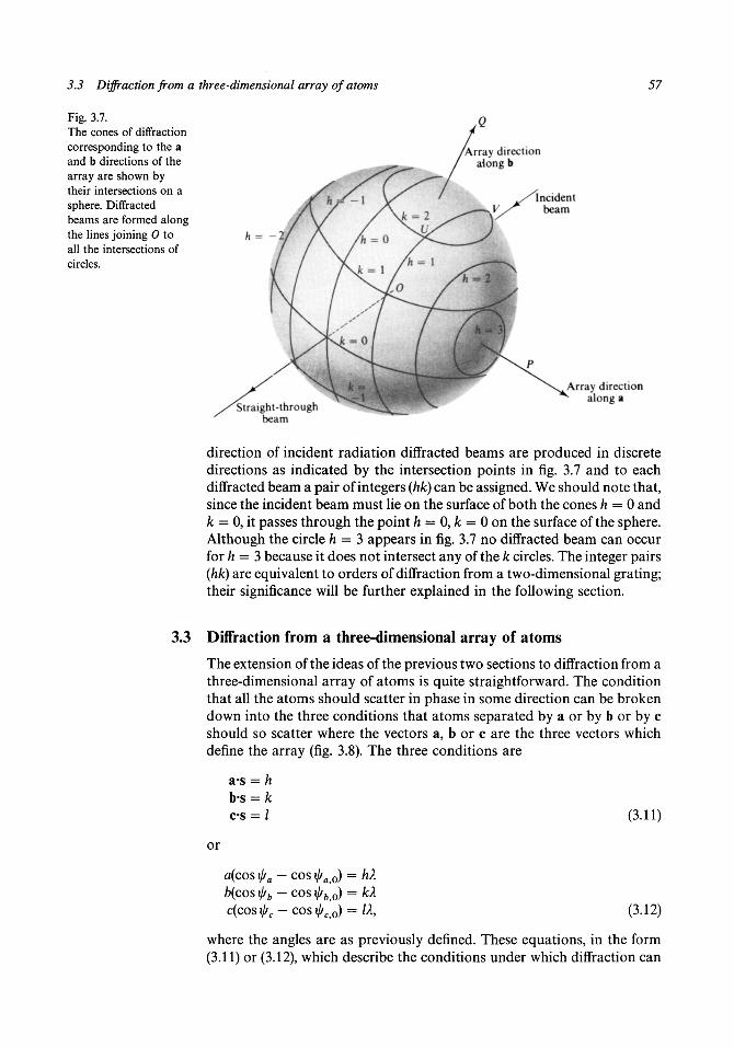
3.3 Diffraction from a three-dimensional array of atoms 57
Fig. 3.7.The cones of diffractioncorresponding to the aand b directions of thearray are shown bytheir intersections on asphere. Diffractedbeams are formed alongthe lines joining 0 toall the intersections ofcircles.
Array directionalong b
Incidentbeam
h = -
Array directionalong a
direction of incident radiation diffracted beams are produced in discretedirections as indicated by the intersection points in fig. 3.7 and to eachdiffracted beam a pair of integers (hk) can be assigned. We should note that,since the incident beam must lie on the surface of both the cones h = 0 andk = 0, it passes through the point h = 0, k = 0 on the surface of the sphere.Although the circle h = 3 appears in fig. 3.7 no diffracted beam can occurfor h = 3 because it does not intersect any of the k circles. The integer pairs(hk) are equivalent to orders of diffraction from a two-dimensional grating;their significance will be further explained in the following section.
3.3 Diffraction from a three-dimensional array of atoms
The extension of the ideas of the previous two sections to diffraction from athree-dimensional array of atoms is quite straightforward. The conditionthat all the atoms should scatter in phase in some direction can be brokendown into the three conditions that atoms separated by a or by b or by cshould so scatter where the vectors a, b or c are the three vectors whichdefine the array (fig. 3.8). The three conditions are
a*s = h
c*s = (3.11)
or
c(cos \j/c — cos Ct0) = U, (3.12)
where the angles are as previously defined. These equations, in the form(3.11) or (3.12), which describe the conditions under which diffraction can

58 Diffraction from a crystal
Fig. 3.8.The relationship ofincident and diffractedX-rays to the vectorswhich define athree-dimensional arrayof atoms.
Incidentray
Diffractedray
take place are known as the Laue equations and they are of centralimportance to the subject of X-ray crystallography.
In fig. 3.9 the cones defined by equation (3.12) are illustrated for a typicalcase by their intercepts with a sphere. We can see now that there is animportant new feature in this figure which has not appeared before. There isno point on the surface of the sphere, except h = 0, k = 0, / = 0, throughwhich passes one member of each of the families of circles and therefore nogeneral diffracted beam can be produced. This will be the normal situationwhen an incident beam has an arbitrary direction in relation to the array.
If we now wish to know what condition does give a diffraction beam wecan approach the problem in two ways. We can stipulate the triplet ofintegers (hkl) and ask ourselves the question - 'How do we select a directionof incident beam (i.e. i/^?0, \\ih 0, \j/c 0) such that the values of ij/a, ij/b and \j/c
given by equations (3.12) are possible directions of a diffracted beam?' Theselatter three angles are to be 'possible' in the sense that for fixed vectors a, band c the angles are not independent and must therefore be related in thecorrect way. Looked at in this way the problem seems a very formidable oneand this is not, in fact, the best way to approach the problem. Rather weshould ask ourselves whether we can find a vector s which satisfiesequations (3.11), since an incident and diffracted direction corresponding tosuch a vector s would be what we are looking for. This approach also showsus another new feature of the problem. The magnitude of the scatteringvector s gives the angle 6 and the incident and diffracted beams must eachmake an angle %n — 6 with s (as in fig. 2.3) and contain s in the plane theydefine. It is clear from fig. 3.10 that the vector So which is along the incidentdirection can lie anywhere along the surface of a cone of semi-angle rc — 9whose axis is the direction of s. We can see from this that if there is anysolution at all to the problem then there is a whole family of solutions. Thatthere is some solution can be appreciated by an examination of fig. 3.9. If thecrystal is rotated about some axis, say the a axis, then the family of conescorresponding to various values of h does not move while the other twofamilies of cones vary. For a particular pair of indices k and / the point ofintersection on the sphere will move as the crystal rotates. Wherever it falls

3.4 The reciprocal lattice 59
Fig. 3.9.The cones of diffractioncorresponding to the a,b and c directions ofthe array are shown bytheir intersections on asphere. A diffractedbeam would beproduced along a linejoining 0 to anytrisection of circles.None occurs in the caseshown (except h = 0,k = 0, / = 0).
Array directionalong c
Array directionJilong a
k =
Array directionalong b
Straight-throughbeam
Fig. 3.10.The conical surface is thelocus of the incident anddiffracted beams for aparticular scatteringvector s. The threevectors §0, s and S mustalways be coplanar.
0
on one of the stationary h circles a diffracted beam will be producedcorresponding to that particular combination of h, k and /.
3.4 The reciprocal lattice
We are now going to consider the Laue equations in the form (3.11) andexamine the problem of finding scattering vectors s which will satisfy theserelationships for a given set of integers (hkl).
Consider the unit cell, defined by the vectors a, b and c and illustrated infig. 3.11. We define a new vector a* by the following relationships:
a**a = 1; a**b = a**c = 0. (3.13)
Since the scalar product of a* with both b and c is zero then it must beperpendicular to each of them (or zero) and is hence perpendicular to the

60 Diffraction from a crystal
Fig. 3.11.The relationship of thereciprocal-lattice vectora* to a, b and c.
plane defined by them. This fixes the direction of a* and its angularrelationship with a. The condition a*#a = 1 then fixes its magnitude and soit is completely defined. Two other vectors, b* and c*, can be similarlydefined and we now have the complete set of relationships
a-a* = 1 a-b* = 0 a-c* = 0ba* = 0 b-b* = 1 be* = 0ca* = 0 cb* = 0 c-c* = 1. (3.14)
Just as the three vectors a, b and c define a space lattice, so the vectors a*,b* and c* define another lattice which is given the name of reciprocal lattice.The 'reciprocal' nature of this lattice as compared to the real space lattice issuggested by the non-zero diagonal elements of the relationships (3.14) andwe shall see that the reciprocal relationship will also show itself in otherways. It is possible to define a point of the reciprocal lattice by three integersgiving the displacement from the origin in units of a*, b* and c*.
Such a reciprocal lattice point can be denoted by the vector ha* +/cb* + /c* where h, k and / are three integers. Now we look at the followingequations:
(ha* + /cb* + /c*)-a = h(ha* + /cb* + /c*)-b = k(ha* + /cb* + /c*)-c = / (3.15)
which follow from the relationships (3.14). Comparing equations (3.15) and(3.11) it is clear that the vector ha* + /cb* + /c* is a possible value of s whichsatisfies the Laue equations for the indices (hkl) and, in fact, it turns out thatthis value is unique. We have now completely solved the problem, inprinciple at any rate, of how to set the crystal to give the (hkl) reflection.First one finds the reciprocal lattice, which is fixed relative to the crystal,and this then gives the scattering vector
s = ha* + /cb* + /c* (3.16)
which, therefore, is also fixed relative to the crystal. The magnitude of s givesthe diffraction angle 20 from equation (2.12) and the crystal (and hence s) ispositioned so that the incident beam makes an angle ^it — 6 with s. Thediffracted beam will then be observed, also making an angle rc — 6 with s,and in the plane defined by the incident beam and s. As we saw from fig. 3.10this does not give a unique relationship between the incident beam and thecrystal.
When space lattices were discussed in §1.7 it was pointed out that,

3.4 The reciprocal lattice 61
although for a particular atomic arrangement the space lattice was fixed,there are an infinity of possible choices of unit cell. It can be shown thatsimilar considerations apply to the reciprocal lattice. The vectors a*, b* andc* by which it is defined are dependent on the non-unique description of thespace lattice in terms of the vectors a, b and c. However it can be shown thatfor a particular space lattice the reciprocal space lattice is unique; if differentvectors a, b and c are chosen to define the real lattice then, althoughdifferent vectors a*, b* and c* will define the reciprocal lattice, the re-ciprocal lattice will be unchanged. This is illustrated in fig. 3.12 for atwo-dimensional example. The space lattice is shown by black dots and thereciprocal lattice by open circles. The vectors a x and hx can be used to definethe space lattice and these lead to vectors a? and b^ describing thereciprocal lattice. Alternatively the space lattice may be described in termsof a2 and b2 and the reciprocal lattice correspondingly in terms of af and bfbut the lattices themselves remain the same.
A unit cell of the crystal can alternatively be defined by the cell edges a, b,c and interaxial angles a, ft, y. Similarly there will be a reciprocal unit cellderived from this which can be defined by a*, b*, c* and a*, /?*, y*. We shallnow derive some relationships involving these quantities.
First let us derive an expression for the volume of the unit cell. This isgiven by the triple-scalar product of the three sides as
K=a*bx c. (3.17)
To give the volume in terms of the scalar quantities a, b, c, a, /?, y, it isadvantageous to express a, b and c in terms of any orthogonal set of unitvectors, i, j and k so that
a = ax\ + aj 4- azkb = bxi + bj + bzk
and
= cxi 4- c j 4- czk. (3.18)
Fig. 3.12.A given space lattice andcorrespondingreciprocal-space latticedescribed in terms ofdifferent unit cells andrelated reciprocal cells.

62 Diffraction from a crystal
The volume of the unit cell can now be written as
V =ax ay az
K by bz(3.19)
ax
Kc.
ay
byr
az
Kc
X
ax
ay
a
ox
by
cx
cy
c.
Wx
a A4- ayay -
f CLyCy H
1- a,
f- a.
A Mxbxbx
bxcx-
^bzbz
Lb2cz
cxax
cxbx
cxcx
+ cyay -
+ cyby -
4" CyCy H
F c z a
Yczb,_
~czcz
The value of a determinant is unchanged if the rows and columns of thedeterminant are interchanged and it therefore follows that
(3.20)
The rules for multiplying determinants are like those for multiplyingmatrices so that
(3.21)
It can be confirmed from the expressions (3.18) that this reduces to
V2= b a bb b e . (3.22)
c*a c*b c*c
If the interaxial angles are a, p and y as defined in table 1.1 (p. 10) then wehave
a*a = a2 b*b = b2 c*c = c2
a*b = b*a = afecosyb#c = c*b = cb cos a
and
c*a = a*c = ac cos p (3.23)
and substitution of these values in equation (3.22) followed by evaluation ofthe determinant gives
V2 = a2b2c2(l — cos2 a — cos2 P — cos2 y + 2 cos a cos p cos y)
or
V= abc(l — cos2 a — cos2/? — cos2y + 2 cos a cos P cos y)*. (3.24)
By similar reasoning we may also find
*. (3.25)
There is a simple relationship between V and F* which is not obviousfrom equations (3.24) and (3.25) but which may be found as follows:
VV* =
ax ay az
bx by bzb*
3.4 The reciprocal lattice 63
=
=
<*>.a*x
"xKaxCx
b-a*
c-a*
++
a
b
c
which, from the
FF* =
1
0
0
0
1
0
aya\
ayb;
ayc*
•b*
•b*
•b*
* + az.3* b Q,* -
" + azb* bxb*x-
+ azc* bxct H
a-c*
b-c*
c#c*
relationships (3.14),
0
0
1
= 1.
f bya* + bzaf
f bybf + bzb?
h byc* + bzc*
gives
cxa$
cxb*x
T CyUy
+ cyb*
+ cyc*
+ czaf
+ czb*
+ czc*
(3.26
This shows once again the reciprocal relationship of the reciprocal lattice tothe real space lattice. Any one of the parameters of the reciprocal lattice maybe expressed in terms of the parameters of the real lattice and vice versa. Forexample we have
a*a* = 1 from the relationships (3.14)
and
b x ca = 1 from the relationships (3.17)
and since a* is parallel to b x c (both these vectors are perpendicular to theplane defined by b and c) then we must have
b x ca * = •
The magnitude of these equal vectors must be equal and hence
be sin aa* =•
(3.27)
(3.28a)
where Fis given by equation (3.24). The real space parameter, a, is similarlyrelated to the reciprocal-lattice parameters. By cyclic permutation of a, b, cand a, /?, y and the corresponding reciprocal-lattice quantities in equation(3.28a) other relationships may be found. We can rewrite equation (3.28a) as
sin a =
and since
we find
sin a = •
~bc
V*a n d c =
V*
y*(3.28b)

64 Diffraction from a crystal
Table 3.1. Summary of relationships
V = abc(l — cos2 a — cos2 p — cos2 y 4- 2 cos a cos /? cos y)}
F* = a*b*c*(l — cos2 a* — cos2 p* — cos2 y* 4- 2 cos a* cos /?* cos y*)*
FF* = 1
be sin a ac sin p afrsiny* ; o* ; *
F* FJ sina*=-a*b*c* sin p* sin y* abc sin psiny
F* VsinP = -l7rzrr———; sin/?* =a*fr*c*sina*siny* ate sin a sin y
Fsiny = .— . ; siny*=-
n^h^n* cin v* cm K*sina*sinj5* abc sin a sin j5
Again by cyclic permutation of the symbols and by interchanging real andreciprocal parameters new equations can be found from equation (3.28b). Asummary of all these relationships is given in table 3.1.
The magnitude of s can be found from equation (3.16), for
s2 = s-s = (fca* + fcb* + /c*)-(/m* + fcb* + /c*)= h2a*2 + fe2fe*2 + / V 2 + 2hka*b*cosy*
4- 2hla*c* cos j8* + 2/c/b*c* cos a*. (3.29)
If we have dealt at some length with the reciprocal lattice and itsproperties it is because of its great importance in X-ray crystallography. It isuseful to think of the crystal having rigidly attached to it a real space latticeand also a reciprocal lattice so that, as the crystal moves, so do the lattices.With this idea in mind many of the concepts of X-ray crystallography canbe understood much more clearly.
3.5 Diffraction from a crystal - the structure factor
We must now look at the details of the arrangement in a crystal structure.This can be pictured as a close-packed three-dimensional array of unit cellswithin each of which there is a similar distribution of atoms. In fig. 3.13 eightunit cells are shown with four atoms in each unit cell; this can be thought ofas a small part of a very large array which forms the complete crystal. If weconsider the atoms labelled A alone then they form a three-dimensionalarray and from this array a non-zero diffracted beam can occur only if theLaue equations are satisfied. The same remarks apply to the array formedby atoms of type B, C or D alone. Thus the total crystal can be divided intofour component intermeshed arrays and the diffraction from the whole

5.5 Diffraction from a crystal - the structure factor 65
Fig. 3.13.A group of eight unitcells containing fouratoms per unit cell.Each atomic type formsa space lattice.
a
/ '
/
/
/
/•A
/
• A /» /
r/
•ry/* A /
//
.A /
A./
/
/
/
/
crystal will be the sum of the contributions from the four components.Hence there will be a diffracted beam from the whole crystal only when theLaue equations are satisfied and the Laue equations can thus be seen to bethe controlling factor for diffraction from any three-dimensional periodicarrangement of atoms.
We shall refer the scattering from each component array of atoms to thatwhich would be obtained from an array of point electrons at the originpoints of the unit cell - marked O in fig. 3.13. The scattering of any one atomA, with respect to an electron at the origin of the cell it occupies, will be/4exp(27iir *s) and the same ratio will apply for all the atoms A with respectto electrons at all the origins. The total scattered amplitude from the crystalwill thus be that from an array of electrons, one at each unit-cell origin,times a factor
/4exp(27iir/1-s) + /Bexp(27tiiys) + /cexp(2n;irc-s) +/Dexp(27iirD-s). (3.30)
The scattering vector s will correspond to a triplet of integers (hkl) and, ifthere are N atoms in the unit cell, we may, in general, write
i= Z /;exp(27Uiys). (3.31)
The quantity Fhkb which we notice is a function of the contents of one unitcell, is called the structure factor and the integers h, k and / are referred to asthe indices of the reflection. We shall see in § 3.6 the reason for referring to thediffracted beam as a reflection and at the same time we shall discover thatthe indices of the reflection are the same as the Miller indices defined in § 1.6.
The composition of the structure factor Fhkl can be seen in a phase-vectordiagram and is shown in fig. 3.14(a). It can be divided into a real andimaginary part and written as
lBhkl
(3.32)
where
(3.33a)

66 Diffraction from a crystal
Fig. 3.14.(a) Phase-vectordiagram for a structurefactor withcontributions from fouratoms.(b) Phase-vectordiagram for a structurefactor corresponding toa centrosymmetricstructure.
Imaginary axis
Akki
/ D
' <t>hki J^^
t2nxL
/
s
• s
Real axis
(a)
Imaginary axis
Real axis
and
(b)
= X/)sin(27tiys). (3.33b)
There is clearly a phase angle <t>hkl associated with Fhkl which is given by
B h k l
Ahki(3.34)
where Bhkl and Ahkl have the signs of sin (j)hkl and cos (j)hkb respectively.

3.6 Bragg's law 67
The intensity of the diffracted beam from the total crystal, consisting as itdoes of large numbers of unit cells, will clearly be proportional to
<^hkl ~ I Fhkl I = A h k l + Bhkl
N N
= 1 1 //)[cos(27tiys)cos(27iiys) -f sin(27tiys)sin(27i;iys)]
orN N
Jf = Y Y //cos[27i(r — r-Vs]. (3.35)
The intensity is thus seen to depend only on the interatomic vectors andnot on the actual atomic coordinates which depend on an arbitrary choiceof origin. This only confirms what we know from physical considerationsanyway, for we could hardly expect the intensity of the diffracted X-raybeam to depend on an arbitrary choice of an origin or an arbitrary unit cell.
An important case, which often occurs, is when the structure has a centreof symmetry. In § 2.6 we noted that for a centrosymmetric distribution ofscattering material the amplitude of scattering is real. Thus for acentrosymmetric unit cell, with the centre of symmetry as origin, theexpression for the structure factor is found by taking only the real part ofequation (3.31) to give
^ = 1 / ^ 0 8 2^/8). (3.36)
This explains why a centrosymmetric unit cell is always referred to acentre of symmetry as origin in the International Tables - a phenomenon wenoticed with the space group P2Jc when we considered that space group in§1-9.
A phase-vector diagram for the structure factor of a centrosymmetricstructure shows very convincingly why the F is real. In fig. 3.14(b) thescattering contribution is taken in turn from pairs of atoms which arecentrosymmetrically related and after every pair of steps in the diagram oneis always back on the real axis.
Other types of symmetry lead to other special forms of the structure-factorequation and this is dealt with in some detail in §7.3.
3.6 Bragg's law
In 1912, von Laue first proposed that X-rays might be diffracted by crystals.At this time it had been deduced indirectly from the geometry of crystalsthat they were almost certainly in the form of a three-dimensional periodicarray of atoms. From the known values of Avogadro's number, atomicweights and crystal densities the average distance apart of the atoms wasfound to be of the order of 1-2 A and it could be presumed that the crystalrepeat distances would be of the order of tens of angstrom units, von Laue

68 Diffraction from a crystal
reasoned that an optical diffraction grating repeat distance was some fewtimes the wavelength of visible light and the same relationship might obtainbetween the repeat distance in a crystal and X-ray wavelengths. Thisinspired prediction was confirmed by Friedrich and Knipping whose X-raypictures, crude by modern standards as they were, caused a stir ofexcitement throughout scientific circles.
In 1913, W.L. Bragg gave the first mathematical explanation of theactual positions of the X-ray diffraction spots. We can follow the main linesof his explanation by considering diffraction by a two-dimensional array ofscatterers as in fig. 3.15. A number of sets of equi-spaced parallel lines areshown which pass through all the scatterers and, according to the Braggpicture, these planes would act as partial reflectors for X-rays. When aparallel wave train falls on a specularly reflecting surface the conditions aresuch that reflection from any two points of the surface will give rays in phasein the reflected beam. In fig. 3.16(a) this can be clearly seen, as the phasedifference for rays reflected from A and B is CB - AD = 0. However thiscondition would be true for any value of 6 and we must now explain why it isonly for special angles that the reflection can occur - as we know fromexperimental observations. To do this we must bring in the distancebetween the parallel reflecting planes. Since reflections from all points inone plane are in phase, it is only necessary to show that reflection from anypoint on one plane is in phase with that from any point on another plane toshow that the total reflection from the two planes is in phase. The twopoints we shall consider are A and A' separated by the distance d which isthe interplane spacing [fig. 3.16(fc)]. The condition for reinforcement isclearly given by
BA' + A'C = nX
where n is an integer. For reasons which will be clearer later we shall only
Fig. 3.15.A selection of sets ofparallel equally spacedlines on which lie allpoints of an array ofscatterers.

3.6 Bragg's law 69
Fig. 3.16.(a) Parallel raysreflected from differentpoints of a plane are inphase after reflection.(b) Parallel raysreflected from points onneighbouring partiallyreflecting planes are inphase when Bragg's lawis obeyed.
//////.A '//
(a)
A'
(b)
consider the case n = 1. From fig. 3.16(fo) we can see that
BA' = A'C = dsinO
giving
2dsin9 = X. (3.37)
This is the expression known as Bragg's law and it gives the permittedangles of reflection, 0, in terms of X and the spacing of the reflecting planes, d.It can be seen now why we refer to the diffracted beams as 'reflections' andwhy the angle between the incident and diffracted beam is denoted by 29and not simply by 9.
If we look at the atom-rich lines in fig. 3.17(a) in terms of the two-dimensional unit cell which is outlined then it can be seen that theycorrespond to directions given by intercepts of a/2 and b/\ on the cell edges.In three dimensions one would have atom-rich planes parallel to the planesdefined by three points with intercepts on the unit-cell axes of a/h, b/k, c/lwhere h, k and / are three integers. These we shall refer to as the indices of theX-ray reflection and the spacing of the planes so defined is denoted by dhkl.In fig. 3.17(a) the indices of the lines shown are (21) and in fig. 3.17(fc) thereare shown the lines with indices (42). Now the latter lines are not all atom-rich - in fact alternate ones are completely empty. In terms of Bragg's lawthe angle 9 corresponding to such a spacing is given by
sin0 =2dA2
but this can also be expressed as
2Xs i n 0 =
2d21
Seen in th is way, a reflection from the line with indices ( 2 x 2 2 x 1 ) can
be r ega rded as a s econd -o rde r reflection (difference of p a t h 2X by reflection
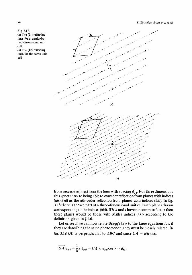
70
Fig. 3.17.(a) The (21) reflectinglines for a particulartwo-dimensional unitcell.(b) The (42) reflectinglines for the same unitcell.
Diffraction from a crystal
(a)
(b)
from successive lines) from the lines with spacing d21. For three dimensionsthis generalizes to being able to consider reflection from planes with indices(nh nk nl) as the nth-order reflection from planes with indices (hkl). In fig.3.18 there is shown part of a three-dimensional unit cell with planes drawncorresponding to the indices (hkl). Ifh, k and / have no common factor thenthese planes would be those with Miller indices (hkl) according to thedefinition given in § 1.6.
Let us see if we can now relate Bragg's law to the Laue equations for, ifthey are describing the same phenomenon, they must be closely related. Infig. 3.18 OD is perpendicular to ABC and since OA = a/fc then
OA-dhkl = j = OAx dhklcosx = dm.
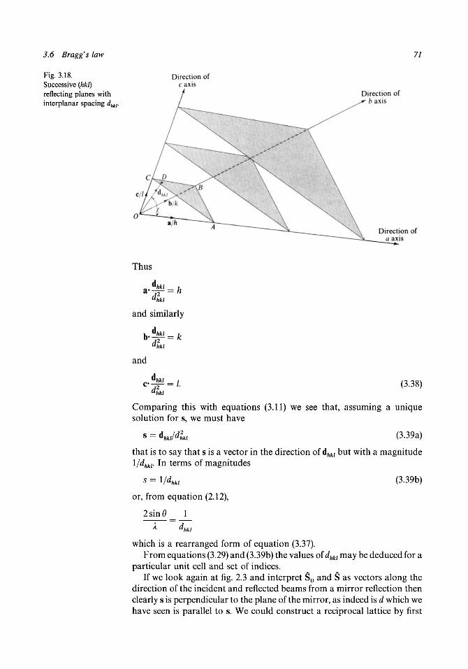
3.6 Bragg's law
Fig. 3.18.Successive (hkl)reflecting planes withinterplanar spacing dhkl.
71
Direction ofb axis
Thus
"hkl
and similarly
dinand
"hkl
d?= 1
hkl
(3.38)
Comparing this with equations (3.11) we see that, assuming a uniquesolution for s, we must have
1 = <V<*few (3.39a)
that is to say that s is a vector in the direction of dhkl but with a magnitudel/dhkl. In terms of magnitudes
5 = l/dhkl
or, from equation (2.12),
2sin0 1
(3.39b)
which is a rearranged form of equation (3.37).From equations (3.29) and (3.39b) the values of dhkl may be deduced for a
particular unit cell and set of indices.If we look again at fig. 2.3 and interpret So and S as vectors along the
direction of the incident and reflected beams from a mirror reflection thenclearly s is perpendicular to the plane of the mirror, as indeed is d which wehave seen is parallel to s. We could construct a reciprocal lattice by first

72 Diffraction from a crystal
drawing planes with intercepts a/h, b/k and c/l, as in fig. 3.18, then findingthe normals to these planes from 0 and then marking the points along thenormal distance 1/d from 0. That this would produce a lattice of points isperhaps not self-evident but the identity of s separately with dhkl/dlkl andwith /za* + fcb* 4- /c* should leave us in no doubt that it would do so.
Thinking of X-ray diffraction in terms of Bragg's law is often veryconvenient and we shall have recourse to this description of the diffractionprocess from time to time. Whether or not one is formally justified inthinking of a diffraction process in terms of specular-type reflection is nottoo certain from the physical point of view but, since the two types ofdescription are mathematically equivalent, there is no harm in doing so.
In the foregoing description of Bragg's law we have treated only the caseof one atom per unit cell; if there are many atoms per cell then one shouldthink in terms of many sets of reflecting planes of spacing dhkl each with adifferent reflecting power and so interleaved that the reflected rays fromeach set interfere with each other. This situation is shown in fig. 3.19 for atwo-dimensional unit cell containing three atoms per unit cell.
3.7 The structure factor in terms of indices of reflection
It is convenient to express the positions of atoms in the unit cell with respectto the chosen origin in terms of fractional coordinates. Thus we say that anatom has coordinates (x, y, z) where x, y and z are three fractional numbersin the range 0-1. If the cell edges are denoted by the vectors a, b and c thenthe vector position of an atom would be
r = xa + yb -f zc (3.40)
as is shown for the point P in fig. 3.20.Previously, in equation (3.16), we have found an expression for s in terms
of h, k and / and now we can rewrite equation (3.31) asN
Fhki= Z /;-exp(27ur/s)
Fig. 3.19.A two-dimensionalstructure with threedifferent atoms showinginterleaved reflectingplanes.

3.7 The structure factor in terms of indices of reflection 73
Fig. 3.20.The relationship of thevector OP = r to thefractional coordinates ofP(x,y,z).
= Z ffixpl2ni(xjBL + yjb + zf)-(h&* + fcb* + /c*)].
From this and the relationships (3.14) we find
Fm = Z ffi*pl2ni(hxj + kyj + bjf]. (3.41)
In the case of a centrosymmetric structure the structure-factor equationappears as
Fhki = Z ffios[2n(hXj + kys + Izj)].
7 = 1
and, using this nomenclature, equation (3.35) becomes
N N
^hu = Z ^ffjcos{2'^[Mxi ~ xj) + Kyi ~ yj) + Kzi •
(3.42)
(3.43)
The experimentally observed intensity of a diffracted beam is proportionalto Jhkl and it can be seen from equation (3.43) that
Shu = Jhki- (3.44)
This equation holds whether or not the crystal structure has a centre ofsymmetry. There is a useful concept of a weighted reciprocal lattice where weassociate with each reciprocal lattice point the corresponding J>m. Equation(3.44) implies that the weighted reciprocal lattice always has a centre ofsymmetry. This important intensity relationship is known as Friedel's law.
The form of the structure-factor equation, (3.41), is the most useful one inpractice, for normally, as we shall see, one wishes to calculate structurefactors when the atomic coordinates (x,y,z) are known for particularindices of reflection (hkl).
In appendix I there is given a FORTRAN® program STRUCFAC whichcan be used to calculate structure factors for any two-dimensional space
74 Diffraction from a crystal
group. It contains facilities, such as provision for anomalous scattering(chapters 6 and 8) and a temperature factor (chapter 6) which have not yetbeen dealt with but these can be ignored for now and the program used tosolve Problems 3.4 and 3.5. The reader should examine the FORTRAN®listing which is liberally provided with COMMENT ' C statements so thatall features of the program may be seen. The output from STRUCFAC isstored in the data file SFl.DAT, the name of which may be changed by theuser. This file should be kept as it may be used as input for Problems toother chapters.
Problems to Chapter 3
3.1 Draw diagrams similar to those shown in fig. 3.2 for a row of sixscatterers at intervals of a*s = 0.05 and plot the resultant amplitude as afunction of a#s.
3.2 A parallel beam of radiation of wavelength X falls on a row of scatterersof spacing 5X so that its direction makes an angle of 30° with the row.Find what orders of diffraction will be produced and the angle thediffracted beams will make with the row.
3.3 A unit cell has the following parameters:
a = 5A b = 10A, c = 15A, a = p = 90°, y = 120°.
(i) Determine the parameters of the reciprocal cell.(ii) Find the volume of the real and reciprocal cells,
(iii) Find the spacing of the (321) planes.(iv) If Cu Koc radiation is used (X = 1.54 A) what is the angle of
diffraction (20) for the (321) reflection?3.4 The crystal and molecular structure of the phenylethylammonium salt
of fosfomycin, C8H12N+.C9H6OPO^.H2O, was solved by A. Peralesand S. Garcia-Blanco (Ada Cryst. (1978) B34 238-42). The non-centrosymmetric monoclinic space group is P2V The cell dimensions are:
a = 11.54 A, b = 6.15A, c = 10.21 A; p = 102.5°,
and the cooordinates of the non-hydrogen atoms (the hydrogen atomswill make a small and negligible contribution to the structure factors) inone asymmetric unit are shown in table 3.2. The projection down the baxis has the centrosymmetric two-dimensional space group p2. If theX-ray wavelength is 1.542 A (Cu Koc radiation) then use the programSTRUCFAC (appendix I) to calculate the complete set of observablestructure factors for this projection.
3.5 The c-axis projection of the phenylethylammonium salt of fosfomycinhas the non-centrosymmetric two-dimensional space group pg. Calculatethe observable structure factors for this projection taking all necessaryinformation from Problem 3.4.
3.6 A crystal of density very near 1.2 x 10³ kgm" 3 is found to have a unitcell with a = 5.601 A, b = 6.002 A, c = 8.994 A, a = 100.7°, p = 95.2°,y= 115.3°.
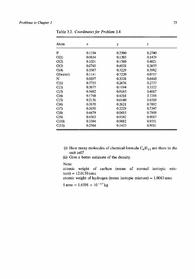
Problems to Chapter 3 75
Table 3.2. Coordinates for Problem 3.4
Atom
PO(l)O(2)O(3)O(4)O(water)NC(l)C(2)C(3)C(4)C(5)C(6)C(7)C(8)C(9)C(10)C(ll)
X
0.11940.06540.10010.07400.35870.11410.06970.27550.36770.34820.17480.21560.26700.36500.44790.43630.33940.2564
y
0.25000.13030.15600.49280.32290.72200.32380.26760.11940.91650.43180.61400.26210.22290.06930.95420.98820.1433
z
0.27400.14790.40210.26550.39820.07170.64100.27370.33220.40170.73180.65190.78920.73470.79090.90170.95510.9011
(i) How many molecules of chemical formula C6H1 2 are there in theunit cell?
(ii) Give a better estimate of the density.
Note:atomic weight of carbon (mean of normal isotopic mix-ture) = 12.0150 amuatomic weight of hydrogen (mean isotopic mixture) = 1.0083 amu
1 amu =1.6598 x 10"2 7kg

4 The Fourier transform
4.1 The Fourier series
Let us consider a function f(X) which is single-valued, continuous (exceptfor a finite number of finite discontinuities), with a finite number of maximaand minima and which is defined in the range \a ^ X ^ - \a. Within thisrange such a function may be represented by a series of sine and cosineterms of the form
i(X) = Ao + 2 Ahcosl2nh— ) + 2i \ a h=l
( XBh sin (27i/2—). (4.1)
This particular form of the series, known as the Fourier series, withfactors of two outside the summation signs, we have adopted because itsimplifies the forms of expressions we shall obtain by subsequentmanipulation. We need not be too troubled by the various mathematicalrestrictions placed on the function f(X); all the functions with which we shallfind ourselves concerned are going to be very well behaved.
We might look at the form of some of the terms which are included in thesummation. In fig. 4.1 there are shown in the range \a ^ X ^ - \a thefunctions cos[2u(Z/a)], cos[27t2(*/a)], sin[27i(Z/a)] and sin[27i2(X/a)]. Itwill be seen that the main characteristic of cos[27i/i(X/a)] is that it is an evenfunction of X whereas sin[2nh(X/ay] is an odd function of X.
If, for a given f(X), we wish to determine the coefficients in equation (4.1)we make use of the following relationships:
to)-2a
Fig. 4.1.The functions cos{2n(X/a)}, cos{2n2(X/a)}, sin{2n(X/a)} and sin{2n2(X/a)}.
76

4.1 The Fourier series 77
ra/2 ( x\cos [2nn— dX = 0 (4.2)
J-a/2 \ <*/for n # 0, where n is an integer;
/ X\cos 2nn— dX = a (4.3)
-a/2 V aJfor n = 0 (since then cos[27in(X/a)] = 1 for all X); and
%a'2 ( x \sin [2nn- dX = 0 (4.4)
/-a/2 \ a)r
for all integers n.The results (4.2) and (4.4) can be seen in fig. 4.1 from the fact that there are
equivalent matching positive and negative regions in the cosine and sinefunctions.
Other results follow from equations (4.2), (4.3) and (4.4). For example,%a/2 ( x \ ( x \
cos I 271/1— Icosl 2nm— )dXI-a/2 V */ Vr\ i cosZ-» - a / 2
2n(n + m)— dX 4- - cos 2n(n - m ) - dX = 0 (4.5)L aJ 2J-a/2 L aJ
unless n = ± m when.a/2 / ^ , -a/2
I cos2f 27 in - )d^ = I i + ^cos(27i2n- ) \dX = \a. (4.6)J-a/2 V aJ J-a/lll ^ V fl/JWe can also find
.a/2
r f x\ f x\sin 27in— I sin 27im— IdX
J-«/2 \ a) \ a)i rfl/2 r -xn i ffl/2 r x~i
= - cos 2u(n - m)— dX - - cos 2n(n + m)— dX = 0 (4.7)2J-a/2 L aA 2J"«/2 L aAunless n= ±m when
.a/2 / v -a/2
sin2 2nn- )dX =\ +\ cos (2n2n- ]\dX = + \a.- « / 2 V a) J-a/2 ~ L2 2 V « / J
(4.8)
The final result we shall require is.a/2
f f x\ ( x\sin [ 2TIM— I cos [ 27im— IdX
J-«/2 V */ V fl/i rfl/2 r x~\ i ra/2 r x i
= - sin 2n(n + m)— dX + - sin 2n(n - m)— dX = 02J-«/2 L a\ 2J-a/2 L "Afor all n and m.
We now note that, for an integer H,

78 The Fourier transform
Ca/2 ( x\ Ca/2 ( x\f (Z)cos[2nH—)dX = A0\ c o s [ 2 % H - dX
J-a/2 V a) J-a/2 \ "Joo [a/2 / y\ / y\
+ 2 £ Ah\ cos [2nh- cos 2 T I # - )dXh=l J-a/2 \ fl/ \ a /
oo pfl /2 / X \ / y\+ 2 X B j sin 2icfc- cos 2icfl- dX (4.10)
fi=l J-a/2 \ a) \ a)
and, from equations (4.5), (4.6) and (4.9), we find that all the components onthe right-hand side are zero except for
Ca/2 ( x\2AH cos2 2nH— )dX = AHa. (4.11)
J-a/2 \ a)Thus we have
.a/2I f ' / X\
AH = -\ f(X)cos(2nH- )dX (4.12)fl J-a/2 V a)
and similarly we find
l Ca/2
BH = -\Ca/2 ( x\\ f(X) sin 2nH - dX. (4.13)J-a/2 V a)
The expression (4.1) can be rewritten as
f(X)= £ ^ c o s ( 2 i i f c - ) + £ Bhsm(2nh-\ (4.14)h=-oo \ a ) h=-oo \ aJ
where A_h = Ah, B_h = — Bh and Bo = 0.What we are doing here is to extend the range of indices to all integers,
both positive and negative. The relationships between the Fourier coefficientwhich are given in equation (4.14) are consistent with what we would obtainfrom equations (4.12) and (4.13) since cos 6 = cos( — 9), sinO =- sin( - 9) and sin 0 = 0.
If we now write
Ch = Ah + iBh (4.15)
then
/ X\ ( XQexp - 2TL/Z— + C_^exp I 2ufc—
V a \ a
+
r ( x\ t x\\(Ah + iBh) cos 2nh— - i sin [2nh—)\
L V a ) \ a)\Y ( x\ ( X\\
(Ah - iBh) cos 2nh— + i sin 2nh —
L V a) \ a)A( x\ ( x
= 2^cos \2nh— + 2B,sin 2u/z —\ a) \ a
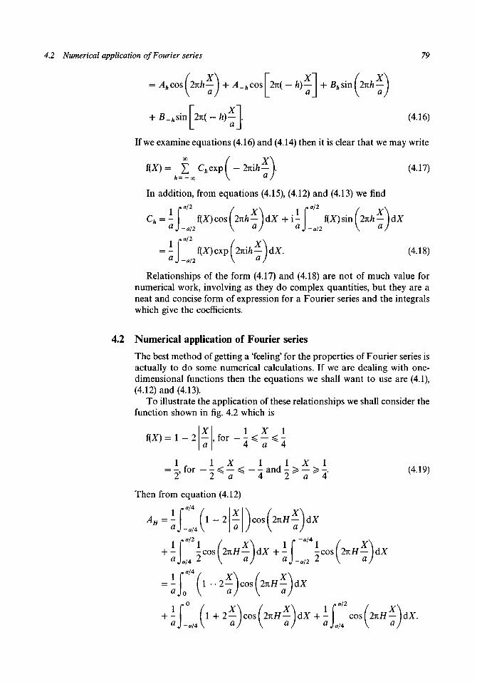
4.2 Numerical application of Fourier series 79
X^x\ f X] ( X= Ahcosi2nh—\ + A_hcos\ 2%(-h)— +^sin( 2nh —
sin 2it( - h)- .+ B_hsm\2n(-h)-\. (4.16)
If we examine equations (4.16) and (4.14) then it is clear that we may write
f(X)= £ CkaJ-2nih-\ (4.17)h=-ao \ aJ
In addition, from equations (4.15), (4.12) and (4.13) we find
l Ca/2 ( x\ l Ca/2 ( x\Ch = -\ f(X)cos[2nh-)dX + i- f(Z)sin (2nh- )dX
aj-a/2 \ ") a)-al2 \ <*)a/2 ( x\
f(X) exp 2nih - dX. (4.18)aJ-a/2 \ «/
Relationships of the form (4.17) and (4.18) are not of much value fornumerical work, involving as they do complex quantities, but they are aneat and concise form of expression for a Fourier series and the integralswhich give the coefficients.
4.2 Numerical application of Fourier series
The best method of getting a 'feeling' for the properties of Fourier series isactually to do some numerical calculations. If we are dealing with one-dimensional functions then the equations we shall want to use are (4.1),(4.12) and (4.13).
To illustrate the application of these relationships we shall consider thefunction shown in fig. 4.2 which is
f(X) = 1 - 2 X 1 X 1, for - - < - < -
4 0 4
= T, for - - < - < - - and - > - > - . (4.19)2 2 a 4 2 a 4
cos [2%H- )dX
J
Then from equation (4.12)
i r"/2i / x\+ - -cos 2TIH- )dX+- I -cos(2nH-)dX
+ - (1+ 2—)cos|2uH—)d^ + M cos|2Ti/f—W-

80 The Fourier transform
XX XX X XX XXX XX XXJ
Fig. 4.2.
The function f{X) = , for -{a
The crosses show the values of the reconstituted function computed from the Fourier serieswith /i = 10.
and these integrations give
AH = T772 V~ C 0 S "V) for H ^ ° and ^o = (4.20)
From equation (4.12) it can be seen that Ao = (I/a) x area under thecurve and this can be confirmed for this simple function by an examinationof fig. 4.2.
If one formally goes through the process of using equation (4.13) todetermine the coefficients BH it would be found that they are all zero. Thiscould be predicted from the fact that f(X) is an even function of X (i.e.f(X) = f( — X)) and the Fourier series which represents it must contain onlyeven (i.e. cosine) terms.
Having obtained the values of the coefficients Ah we are now in a positionto see how well we can synthesize f(X) from
= Ao + 2 V A,.cos 2nh— .
The coefficients, ^1 , for h = 0 to 10 are:
h 0 1 2 3 4 5 6
(4.21)
10
0.1013 0.01130.6250 0.0506 0
0.0041 0.0021 0.00130.0056 0 0.0020
In practice one must always terminate the summation at some point andthe similarity of the computed f(X) to the true function will depend on thenumber of terms in the summation. In fig. 4.3 there are shown the results ofterminating with hmax = 1, 3 and 7 and in fig. 4.2 the result of havingftmax = 10. It can be seen how the summation gradually evolves towards thecorrect shape and the result with h = 10 is a very good representation of the

4.2 Numerical application of Fourier series 81
-a/2
-a/2
(c) hmax = 7
-a/2
0
f(x)
1.0
-0.5
0
all
a/2
Fig. 4.3.Simulation of the function shown in fig. 4.2 using a Fourier series with: (a) hmax = 1; (b)hmax = 3 (since A4 = BA — 0 this is equivalent to hmax = 4); and (c) hmax = 7. The computedvalues are shown by dots.
function; indeed, one could represent the function by the summation withany desired degree of precision by increasing the number of terms. Evenhmax = 3 gives quite a good reproduction of i(X) with the main discrepancybeing in the region of the origin. The summations shown in fig. 4.3 weremade with the computer program FOUR1 given in appendix II. It is a verysimple program, written to be easy to understand; it exploits the symmetryof cosine and sine functions in that the former are even functions, so thatf( _ X) = f(X) and the latter are odd, so that f(-X) = - f(X).
In the early days of crystallography, before electronic computers wereavailable, the task of computing a Fourier series - which can be in morethan one dimension - was a formidable one. An early and importantcontribution to this problem was made by Beevers and Lipson (1934) whoprecalculated components of individual contributions to the series on stripsof cardboard which were provided in convenient-to-use wooden boxes. In

82 The Fourier transform
Fig. 4.4.A typicalBeevers-Lipson stripgiving-31cos(27t x 19 x n/60)where n is from 0 to 15.CE indicates that it is acosine strip for evenY^ths. The odd ^ t h sare on the reverse side.As a check for the userthe last figures is thesum of the 16 values.
Fig. 4.5.The periodic functionreproduced by theFourier series which isderived from thefunction i(X) shown infig. 4.2.
addition to the even and odd symmetry of cosine and sine functions it willbe seen from fig. 4.1 that the functions are completely defined in the range 0to \a and the way that the complete range is generated from the partialrange depends both on whether it is a sine or a cosine and also on the parityof h. A typical Beevers-Lipson strip is shown in fig. 4.4. The strip gives thevalue of — 31 cos(27i x 19 x n/60) where n goes from 0 to 15, which is theequivalent of going from 0 to \a in steps of a/60. By placing strips undereach other, one could conveniently do the summations over the quarterrange separately for cosine (odd h), cosine (even h), sine (odd h) and sine(even h) which could then be combined using symmetry to give the wholerange.
31 CE 19 31 13 21 29 3 27 25 6 30 18 15 31 10 23 28 0 (4) |
Let us now examine the properties of the Fourier series, equation (4.1), ina little more detail. The first thing we notice is that although we haveoriginally stated that f(X) is defined in the range — a/2 ^ X ^ a/2 the seriescan be summed for values of X outside this range. From the properties ofthe sine and cosine functions it is clear that the series has the same value forX = Xl9 for X = Xx + a and, indeed, for X = Xx + ma where m is anyinteger. Thus the summation gives a periodic function of spacing a and theFourier coefficients Ah corresponding to the f(X) shown in fig. 4.2 actuallyreproduce the periodic function shown in fig. 4.5.
Often it is convenient to define a function in the range of X from 0 to aand it is clear that the Fourier series can be applied to this range. Thecoefficients Ah which reproduced the f(X) defined in the range — a/2 ^ X^ a/2 in fig. 4.2 also reproduce the function f(X) defined in the range
0 ^ X ^ a as shown in fig. 4.5. One may replace all the limits a/2, -a/2 bya,0 in the relationships (4.2) to (4.13).
It is also convenient to change from the variable X which has the units ofa to the variable x = X/a so that x is now a fractional coordinate defined inthe range \^x^ — ^ o r l ^ x ^ O .
Let us suppose that we have a periodic function f(x) but that f(x) is nownot an analytical function but one which is known in graphical or tabular form.
Such a function, whose periodicity is unity is shown in fig. 4.6 bothgraphically and also tabulated at intervals of in x. We wish to carry outby a numerical method the integrals
f(x)cos(27i/zx)dx (4.22a)

4.3 Fourier series in two and three dimensions 83
60x
0123456789
f(x)
50515254576063666972
60x
10111213141516171819
f(x)
76798183848585848380
60x
20212223242526272829
f(x)
79767370666360555047
60x
30313233343536373839
f(x)
42393734323541516274
60x
40414243444546474849
f(x)
90106117123126126123120113104
60x
5051525354555657585960
f(x)
9585787165605652515050
(a)Fig. 4.6.A non-analytical function f(x) shown graphically and by a table.
and
Bh= (4.22b)
There are various methods available for numerical integration and inappendix III there is given a simple program, SIMP1, for applying TheSimpson's Rule method. This replaces an integral
h N
by - £ wB nh)
where the range of x values, from a to b is divided into an even number ofintervals N each of width h and the weights wn follow the pattern1 4 2 4 2 . . . 2 4 2 4 1 . Simpson's Rule is equivalent to adding the areas ofparabolae fitted to three function values at points defining successive pairsof intervals. Using this method the integrals in equation (4.22) can bereplaced by the summations
and
6 0
6 0
(4.23a)
(4.23b)
The coefficients obtained from these summations are shown in table 4.1 upto h= 15 and these values of Ah and Bh are used with FOUR1 toreconstitute the function f(x) which is shown in table 4.2. These results maybe compared with the tabulated values of the original function given in fig.4.6. The small disagreements are due to rounding off the calculated values ofAh and Bh and the termination of the series.
4.3 Fourier series in two and three dimensions
The Fourier series can also be used to express two- and three-dimensionalfunctions. For example if we have a two-dimensional, single-valued and
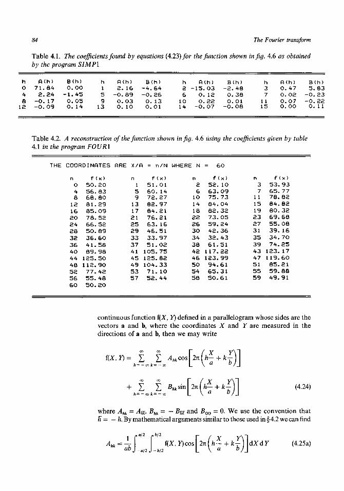
84 The Fourier transform
Table 4.1. The coefficients found by equations (4.23) for the function shown in fig. 4.6 as obtainedby the program SIM PI
h04
a12
P(h)71. 842. 24
-0. 17-0.09
B(h)0.00
-1.450. 050. 14
h15913
A(h)2. 16
-0.890. 030. 10
B(h)-4. 64-0. 260. 130.01
h261014
A(h>-15.03
0. 120. 22
-0. 07
B(h)-2. 480. 380. 01
-0.08
h371 115
A(h>0. 470. 020.070. 00
B5.
-0.-0.0.
(h)83232211
Table 4.2. A reconstruction of the function shown in fig. 4.6 using the coefficients given by table4.1 in the program F0UR1
THE COORDINATES
n04612162024283236404448525660
f (x)50. 2056. 8368. 8081.2985. 0978.5266. 5250. 8936. 6041.5889. 98125.50112.9077. 4255. 4850.20
ORE X/ft
n159131721252933374145495357
= n/N
f <x>51. 0160. 1472.2782. 9784.2176.2163. 1646.5133.9751. 02105.75125.82104.3371. 1052. 44
WHERE N
n2610141822263034384246505458
= 60
f (x)52. 1063.0975. 7384. 0482. 3273. 0559.2442. 3632. 4361.51117.22123.9994.6165. 3150. 61
n3711151923273135394347515559
f (x)53. 9365. 7778.8284.8280. 3269. 6855.0839. 1634. 7074.25123.17119.6085.2159. 8849. 91
continuous function f(X, Y) defined in a parallelogram whose sides are thevectors a and b, where the coordinates X and Y are measured in thedirections of a and b, then we may write
f(X,Y)= £ £ AhkcoSfc=-oofc=-oo
r / x y\2ii(h- + k-L \ " D
(4.24)
where Ahk = Aa, Bhk = — B^ and Boo = 0. We use the convention thatH = — h. By mathematical arguments similar to those used in § 4.2 we can find
i c12 cb'2 r / x Y\IA hk = — f(X, F)cos 2TI / I - + k-\ \dXdY (4.25a)
^J- f l /2J-fc/2 L V a h)\

4.4 The Fourier transform 85
and
i c"12 r 6 / 2 r / x Y\IBhk = — f(X, Y)sin \2% [h- + k-\ \dXdY. (4.25b)
If we write
C» = 4 * + iBhk (4.26)
then we have
f(X, Y) = Y V C ^ e x p - 2 7 i i [ h — + k T ) \ (4.27)li= — oofc= — oo L \ / A
and
l Ca/2 Cb/2 V f x Y\lChk = —\ PMOexp 2 u i U - + /c- d ^ d r . (4.28)
ab J -a/2 J -b/2 L V ^ /JThere are corresponding equations for a three-dimensional Fourier
series applied to a function f(X, Y, Z) defined in the parallelepiped given bythe vectors a, b and c.
The final equations corresponding to (4.27) and (4.28) are
f(X,Y,Z)= t t 1h=-a0k=-O0i=-O0
and
=-Lf/2 r r,abc J _a/2 J -b/2J -c/2
exp|27ii( h- + k-f+ I- MdXdYdZ. (4.30)
L V a b c ) \In fig. 4.1 are shown the forms of some of the terms included in a
one-dimensional Fourier summation. It is not quite so straightforward torepresent the terms in a two- or three-dimensional Fourier summation. Thecontours corresponding to cos{27i[3(X/a) + 2(Y/ft)]} = 1, 0 and - 1 areshown in the X Y plane in fig. 4J(a) and the planes corresponding tocos{27t[3(X/a) + (Y/b) + 2(Z/c)]} = 1, 0 and - 1 are shown in fig. 4.7(fe) inrelation to the volume defined by a X ^ 0, b F ^ O and c Z 0.
4.4 The Fourier transform
We have seen that although the functions we have been representing by aFourier series were defined in some one-, two- or three-dimensional regionof space the series itself had a periodic nature. If in equations (4.17) and(4.18) we change our variable of summation from h to s = h/a and makeF(s) = aCh, then
f(X) = -fj F(s) exp( - 2nisX) (4.31)

86 The Fourier transform
(a)
YFig. 4.7.(a) Contours in the X Y plane of
tb)
s 2re( 3—h 2—1 = 1 (thick full line)L V a b)\
= 0 (thin full line)
= — 1 (thick broken line).
Negative regions are shaded.
(b) Intersections of the faces of a unit cell with planes for whichf / X Y ZY]
cos 2it I 3— + - + 2 - I = 1 (thick full line)L V a b c / J
= 0 (thin full line)= — 1 (thick broken line).
Negative regions are shaded.
and
a/2
f(X) exp(27iisX) dX.•a/2
(4.32)
Now let us consider what happens when a becomes very large. Thediscrete values of s ( = h/a) become very close together and values of F(s)

4.4 The Fourier transform 87
determined from equation (4.32) for neighbouring values of s should not bevery different. The sum in equation (4.31) is clearly a real quantity (seeequation (4.14)) and thus can be expressed as
art(4.33)
where R(z) means the real part of z. In fig. 4.8 there is shown, for a particularvalue of X, a typical set of R{F(s)exp( - 2nisX)} for s = 0, ± I/a, ± 2/a, etc.The rectangular blocks have areas (l/«)R{F(s)exp( — 2nisX)} and the totalarea of these blocks from s = — oo to s = + oo will equal f(X). But if a isvery large, or as a tends to infinity, so F(s) tends to be a function of acontinuously variable s and one will then have
f(X) -f R{F(s) exp( - 2nisX)}ds. (4.34)
However we may now take out the 'real-part' symbol within the integrationfor the integral will still be real without this (see equation (4.16)). Thus wehave as a -• oo
and
-J""f
J - a
F(s) exp( -
exp(2nisX)dX.
(4.35)
(4.36)
A function f(X) related to F(s) in the way shown is defined as the Fouriertransform of F(s) and similarly F(s) is the Fourier transform of f(X).Sometimes the integral in equation (4.36) is called the inverse Fouriertransform to indicate the difference between the two forms. On this point itshould be stressed that if the transformation from f(X) to F(s) involves anegative sign in the exponential term then the back transformation from
R{F(s)exp(-27risX)j
7 6 5 4 3 2 1
a a a a a a a
1 2 3 4 5 6 7
a a a a a a a
Fig. 4.8.Values of R{F(s)exp(-27iisX)} at s = 0, ±(l/a), ± ( 2 / 4 The sum of the areas of the blocksgives f(X).

88 The Fourier transform
F(s) to f(X) must have a corresponding positive sign. The two signs can bothbe reversed - this is only a matter of the way the transformation is defined inthe first place in equation (4.15) where one could also have takenCh = Ah- iBh.
We shall now generalize our description of Fourier transforms to thethree-dimensional function given in equations (4.29) and (4.30). Theposition of a point in the parallelepiped whose sides are the vectors a, b andc may be represented by
r = Za + Y 6 + Zt (4.37)
where a, 6 and c are the unit vectors in the directions of a, b and c. This mayalso be written as
r = X-+ Y- + Z-. (4.38)a b c
Corresponding to a, b and c there will be reciprocal vectors a*, b* and c*defined by the equations (3.14) and we may define a vector s by
s = fta* + fcb* + Zc*. (4.39)
If we now write F(s) = VChkl then by similar arguments which lead toequations (4.35) and (4.36) we find
f(r)= F(s) exp( - 2TUST) dv* (4.40)J V*
and
F(s)= f(r) exp(27iis-r) dv (4.41)
In equations (4.40) and (4.41) f(r) represents a function of position in somespace represented by the vector r in which an element of volume is dv. TheFourier transform of f(r) is F(s), a function in a reciprocal space in which anelement of volume is dv*. We can see the mutually reciprocal nature of thetwo quantities r and s from the relationships (4.38) and (4.39).
To illustrate the calculation of a Fourier transform we consider first theone-dimensional function
ry "v/"\ 1 -f 1 ^ V <»-' 1
f(X) = 0 for | X | > \a
which is shown in fig. 4.9(a). The Fourier transform is given by
F(s)= '
= ™ ^ . (4.42)US
The function F(s) is shown in fig. 4.9(fo); it will be noticed that the width ofthe central maximum of F(s), between the two points at which it falls to zero,is 2/a and is thus reciprocally related to the width of the function f(X). This isa characteristic relationship between a function and its Fourier transform;

4.4 The Fourier transform 89
-1.0-
-J— x0(a)
f(X)
2.0'
-\a 0
(c)
Fig. 4.9.(a) The function = 1, -\a <: \a (c) The function f(X) = 2, -\a ^ X ^ \a
= §,\X\>\a.(b) The Fourier transform of the function shown in (a) (d) The Fourier transform of the function shown in (c)
F(s) = - F(s)=

90 The Fourier transform
if the lateral scale of the function changes by a factor fc then the transformchanges by a factor l/fc. We can see this by considering the transforms oftwo functions fx(X) and f2(X), where
ft(X) = kf2(kX). (4.43)
The function f2(X) has l/fc times the lateral spread of f X(Z) and is scaled by afactor k so that
The Fourier transform of f^X) is given by
f00
Fx(s) = f^X) exp(2nisX) dX
= k f2(fcX) exp(27iisZ) dX. (4.44)J - o o
If in the integral (4.44) we substitute kX = rj we find
F1(s) = | f2(!,)exp(2*i!>,)di, = F 2 ( 0 (4.45)
Thus when f2(X) has l/fc times the lateral spread of f^X) we find that F2(s)has k times the lateral spread of Fx(s). This is illustrated in fig. 4.9(c) and (d)which show
f(Z) = 2for -ia^X^iaOfor \X\ >{a (4.46)
and the corresponding Fourier transform
F(s) = -. (4.47)us
There are a number of analytic functions whose Fourier transforms are ofinterest. The Gaussian function
(4.48)
which is normalized to have unit area under the curve has a Fourier transform
F(s) = exp( - 2n2a2s2) (4.49)
which is another Gaussian function. In fig. 4.10 the Gaussian functions(4.48) for a = 1,2 and 3 are shown together with the corresponding Fouriertransforms. The inverse relationship of the width of these functions can bereadily seen.
Another function of great importance to the study of X-ray diffraction isthe Dirac ^-function. This function has the following properties:
d(X) = 0, for X # 05(0) = oo
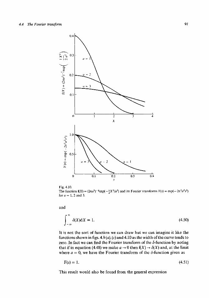
4.4 The Fourier transform 91
0.4
0 ,
0.2
0.1
\
\
a —
^ n =
a =-
-
l\
2 \
3 y ^ ^
1.0
0.5
2
X
0.1 0.2s
0.3 0.4
Fig. 4.10.The function f(X) = (2na2)~±exp(-jX2/a2) and its Fourier transforms F(s) = exp(-27tVs2)for a = 1, 2 and 3.
and
5(X)dX = 1. (4.50)
It is not the sort of function we can draw but we can imagine it like thefunctions shown in figs. 4.9 (a), (c) and 4.10 as the width of the curve tends tozero. In fact we can find the Fourier transform of the ^-function by notingthat if in equation (4.48) we make a -> 0 then i(X) -> S(X) and, at the limitwhere a = 0, we have the Fourier transform of the 5-function given as
F(s) = 1.
This result would also be found from the general expression
(4.51)

92 The Fourier transform
j: d(X)<l)(X)dX = 4>(0) (4.52)
which is a fairly obvious result. Then if we take
cj)(X) = exp(2%isX)
we have
<5(Z)exp(2iusX)dX = exp(O) = 1.D
We can have a 5-function located at a point other than the origin. Thus ifwe have
f(X) = 8(X - a) (4.53)
then this represents a (5-function at X = a. The Fourier transform of this is
- j :F(s)= S(X - a)Qxp(2nisX)dX
-j: <5(X)exp[27tis(X
which, from (4.52), gives
F(s) = exp(2nisa). (4.54)
The functions d(X), S(X — a) and various composite functions derivedfrom the ^-function are illustrated schematically in fig. 4.11 together withthe corresponding Fourier transforms. Of particular interest is the set of^-functions defining a one-dimensional lattice of spacing a where it will benoticed that the transform is another set of ^-functions of weight I/adefining a lattice which is reciprocally related to the first. This result can beextended to three dimensions. A set of (5-functions located at the nodes of aninfinite three-dimensional lattice defined by the vectors a, b and c may berepresented by
fW= t t t 5[r - (nia + n2b + n3c)]. (4.55)«i = — oo n2— — o o « 3 = — oo
The Fourier transform of equation (4.55) is
F ( s ) = 4 I I I 5 [ s - (/ia* + fcb* + / c * ) ] (4.56)f i = — oo k= — cc 1= — oo
a set of ^-functions at the nodes of the lattice which is reciprocal to thatdefined by a, b and c (as defined by the relationships (3.14)) and with weight1/ V where V = a*b Ac. The function f(r) and F(s) are related by the equations(4.40) and (4.41) which give the general relationship between any three-dimensional function and its Fourier transform.
4.5 Diffraction and the Fourier transform
In equation (2.17) the amplitude of scattering from a distribution of nscatterers was found to be

4.5 Diffraction and the Fourier transform 93
Fig. 4.11.Various compositefunctions involving^-functions and theirFourier transforms.
o x(5-function at origin
F(s)
1
0
F(s) = 1
HX)
0 a x
(^-function at X = a
Real part
^ \ )1 \ \ /
F(s)
0
-
Imaginary part
\ \ /I
A'aF(s) =
a a x 1<5-functions at X = a and X = - a " ~a
Infinite array of ^-functionsof spacing a
1 1
a a
Infinite array of ^-functions ofspacing I/a and weight I/a.
(4.57)
where [rj(20,D)]j is the amplitude of scattering at a distance D from thejthscatterer at an angle 26 with the incident radiation. If we have a continuousdistribution of electron density p(r), expressed in electrons per unit volume,then we can imagine that our space is divided into a number of small

94 The Fourier transform
volumes dv within each of which there is an effective point charge p(r)dvelectrons. Thus the scattered amplitude from such a small volume will bep(r)dv times as much as that from an electron at the same position. Fromthis we find that the total scattered amplitude from the distribution ofelectron density p(r), expressed as a fraction of that from a point electron atthe origin, is given by
F(s)= p(r) exp(27iis-r) di; (4.58)Jv
where the integration is over the whole volume of space in which p(r) isnon-zero. If equation (4.58) is compared with equation (4.41) it is clear thatF(s) is the Fourier transform of p(r). We can also infer from equation (4.40)that the inverse transformation is also valid and that
p(r)= F(s) exp( - 2nis-r) dv* (4.59)J V*
where the integration is carried out over the entire volume of the reciprocalspace in which s is defined.
The relationship between diffraction and Fourier-transform theory hasnow been established and the application of Fourier-transform ideas to theconsideration of X-ray diffraction will be found to be most useful.
4.6 Convolution
Let us consider two functions f(X) and g(X). The convolution of these twofunctions is defined by
c(X)= f(u)g(X - u)du. (4.60a)J — oo
By substituting u = X — v and then v = u we find also. 0 0
c(X)= g(u)f{X - u)du. (4.60b)
The operation of convolution is represented by the symbol * and we maywrite
c(X) = f(X)*g(X) = g(X)*f(X). (4.61)
To understand what is meant by the convolution process let us take thetwo functions f(w) and g(w) shown in fig. 4.12(a). For a particular value X theformation of the function g(X — u) is also shown in fig. 4.12(b); it will be seenthat this function may be produced from g(w) by (i) inversion about the pointu = X and (ii) translation of this point to the origin. The operation by whichg(X — u) is produced from g(u) is referred to as folding g(w) about X. In fig.4.12(c) there are shown superimposed the function f(w), g(X — u) and theirproduct f(w) g(X — u). Then the integral (4.60a) which defines c(X) is givenby the shaded area. The result of doing this for all values of X completelydefines the function c(X) and, for the particular example we have considered,this is shown in fig. 4.12(d).

4.6 Convolution 95
(a)
\%(X-u)
0 X
(b)
c(X) =
Fig. 4.12.(a) Functions f(w) and g(u).{b) The function g(X - u).(c) The derivation of f(u)g(X - u). The shaded area gives c(X) = f(X)*g{X).(d) The complete function c(X) = f(X)*g(X).
Another method, which can be used to determine the whole functionc(X) at once, is to express c(X) as a summation by
c(X) = f f(u)g(X - u)du =J
- un)dudu—>0
where the summation is for the n values of un at the centres of the strips ofwidth du which cover the non-zero ranges of the function f(w). The steps inthe process are:
(i) Divide f(w) into strips of width du.(ii) Find the areas of the strips <52In = f(un)du.(iii) Plot g(w)<52ln with origin at centre of nth strip for all n.(iv) Add the resultant curves to obtain c(X).

96 The Fourier transform
Fig. 4.13.(a) g(w) divided intostrips of width 3u.(b) The superposition ofthe functionsf(w - Mjg(Mj<5w.(c) The sum of thesuperimposed functionsrescaled to agree withfig. 4.12(4
This process is illustrated in fig. 4.13 where, for convenience, the roles ofthe functions have been reversed. In (a) there is shown the division of g(w)into eight strips and the relative areas are given. In (b) the eight weightedand displaced images of f(w) are shown and in (c) they are added to give thetotal function c(X).
There is a theorem, the convolution theorem, which is of particularinterest to crystallographers. This states that if there are two functions f(X)and g(X) whose Fourier transforms are F(s) and G(s) then the Fouriertransform of c(X) = f(X)*g(X) is C(s) = F(s)G(s). The proof of this result isfairly straightforward and is now given.
From equation (4.36) we have
C(s) -rJ - c
c(X) exp(27iisZ) dX
which, from equation (4.60b) gives/% oo i% oo
C(s) = f(X - u)g(u) exp(27iisX) du dX.J — oo J — oo
This may be rewritten as
(4.62)
(4.63)
i = g(w) exp(2jisw) f(X - w) exp{27iis(X - u)}dX \du.JU= -GO L J - 0 0 J
(4.64)
859063I
(a)
f{u-un)g(un)Su
U\ "3 U5 "7U2 U4 U6

4.6 Convolution 97
The integral in the square brackets is independent of u (substitutey = x — u) and equals F(s) and it follows that
C(5) = ¥(s)G(s). (4.65)
It may be deduced from the reciprocal nature of Fourier transforms thatc(X) is the transform of C(s) and is also the transform of the productF(s)G(s). Thus we have the general result that the Fourier transform of aproduct of functions is the convolution of the transforms of the individualfunctions. We can express this as
or rJ - c
F(s)G(s) exp( - 2niXs) ds = f(X)*g(X).
f(X)g(X) exp(27iiXs) dX = F(s)*G(s).
(4.66)
(4.67)
Let us look again at the process of convolution and in particular the caseshown in fig. 4.14 where the function g(X) is a spiky function of very smallwidth. If the function g(X) is normalized to have unit area under the curvethen the convolution c(X) differs very little from f(X). If we take this processto the limit so that g(X) = 8(X) then we should find that c(X) = f(X). Thiscan also be found by applying the expression (4.52) since
• j :
g(u)f(X - u)du
8(u)f(X - u)du = f(X). (4.68)
Fig. 4.14.The convolution of f(X)and g{X), a spikyfunction with unit areaunder the curve, is littledifferent from f(X).
f(X)
(X) = f ( A > g m

98 The Fourier transform
Extending the application of equation (4.52) we can determine theconvolution of f(X) with 5(X - a). This is
c(X)= d(u - a)f(X - u) duJ — oo
= f(X-a)
and this result is illustrated in fig. 4.15.
(4.69)
Fig. 4.15.The convolution ofwith a ^-function not atthe origin.
c(X)
0 a
This process is taken another stage by considering the convolution off(X) with an infinite linear array of 8 functions given by
Fig. 4.16.The convolution of f(X)with a ^-function array.
g(X)= X d(X-na).n = — oo
The convolution is given by
c(X)= £ f(X-na)
(4.70)
(4.71)
and c(X) is a periodic function of spacing a. What is more if f(X) iscompletely defined in the range 0 ^ X < a (or any range of width a) then aunit of c(X) is identical in appearance with f(X) in the defined range. Thispoint is illustrated in fig. 4.16. Thus it may be seen that any periodic patternof spacing a may be considered as the convolution of one unit of the patternwith a (5-function at the nodes of a lattice of spacing a. The result may beextended to three dimensions. A three-dimensional periodic function maybe considered as the convolution of one unit of the pattern, containedwithin the parallelepiped defined by the vectors a, b and c, with a set of
4.8 The electron-density equation 99
^-functions at the nodes of a three-dimensional lattice defined by thevectors a, b and c. In particular, the electron density within a crystal may beconsidered as the convolution of the density within one unit cell with thethree-dimensional real-space lattice of spacing a, b and c.
4.7 Diffraction by a periodic distribution
In §4.5 the relationship between diffraction and the Fourier transform wasestablished and this is exemplified by equations (4.58) and (4.59). Thescattered amplitude, as a fraction of that scattered by a point electron, is theFourier transform of the electron density. Thus, from equation (4.65) andthe periodic nature of the electron density in the crystal, the scatteredamplitude is seen to be the product of the transform of the electron densitywithin one unit cell of the crystal with the transform of a set of -functions atthe nodes of a unit-cell lattice which covers the volume of the crystal. Thetransform of this set of (5-functions will, for all practical purposes, be thesame as the transform of an infinite set - that is another set of -functions atthe nodes of the reciprocal lattice. Thus the diffracted amplitude for thewhole crystal can be thought of as the Fourier transform of the electrondensity in one unit cell of the crystal, F(s), sampled at points of the reciprocallattice, s = /ia* + /cb* + /c*. Since the weight associated with each of thereciprocal-lattice 5-function points is 1/K(see equation (4.56)) the scatteredamplitude corresponding to the point (hkl) of the reciprocal lattice is givenby (l/V)Fhkl where the reciprocal-lattice vector is now indicated by thetriplet of integers (we write F(s) = Fhkl).
If the diffracted amplitudes are expressed as a fraction of that from anarray of point electrons at the chosen origins then F ^ is the structure factoras defined in § 3.5. The structure factor is also given by equation (4.58) if theintegration is carried out over the volume of the unit cell and if p(r) isexpressed in electron units per unit volume.
4.8 The electron-density equation
In equation (4.59) an expression has been given for the electron density in acrystal in terms of the scattering amplitudes F(s) expressed as a fraction ofthe scattering from a point electron. For the whole crystal, assumed to beinfinite in extent, F(s) exists only at reciprocal lattice points and has weightat these points equal to (l/V)Fhkl.
Thus we may take equation (4.71),
p(r) = F(s) exp( — 2TUST) dt;*,J V*
and replace it by
P « = i I I I F»ki exp( - 2iris-r). (4.72)h= — oo k= — ao 1= — oo
In this equation if Fhkl is the normal structure factor then p(r) will be theelectron density expressed in electrons per unit volume. The electron
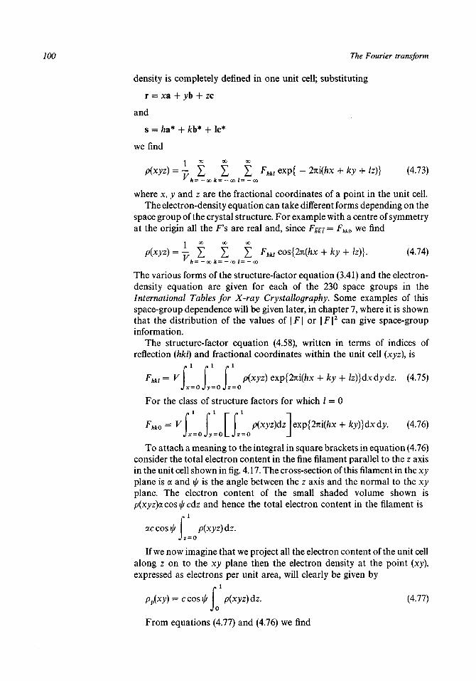
100 The Fourier transform
density is completely defined in one unit cell; substituting
r = xa + yb + zc
and
s = /m* + fcb* + lc*
we find
= ± t i t FhklQxp{-2ni(hx + ky + lz)} (4.73)h= — ao k= — co 1= — oo
where x, y and z are the fractional coordinates of a point in the unit cell.The electron-density equation can take different forms depending on the
space group of the crystal structure. For example with a centre of symmetryat the origin all the F's are real and, since FJ^J = Fhkh we find
^ t t t FhklCos{2n(hx + ky + lz)}. (4.74)h = — o o f c = — o o i = — oo
The various forms of the structure-factor equation (3.41) and the electron-density equation are given for each of the 230 space groups in theInternational Tables for X-ray Crystallography. Some examples of thisspace-group dependence will be given later, in chapter 7, where it is shownthat the distribution of the values of | F | or \F\2 can give space-groupinformation.
The structure-factor equation (4.58), written in terms of indices ofreflection (hkl) and fractional coordinates within the unit cell (xyz), is
hkl -'J1 ITJx = 0 Jy = O Jz = C
p(xyz) exp{2iii(hx + ky -f /z)}dxdydz. (4.75)
For the class of structure factors for which / = 0
r1 r1 r r1 iF h k 0 = V \ p(xyz)dz exp{27ti(/*x + ky)}dxdy. (4.76)
To attach a meaning to the integral in square brackets in equation (4.76)consider the total electron content in the fine filament parallel to the z axisin the unit cell shown in fig. 4.17. The cross-section of this filament in the xyplane is a and \// is the angle between the z axis and the normal to the xyplane. The electron content of the small shaded volume shown isp(xyz)a cos \\t cdz and hence the total electron content in the filament is
p(xyz)dz.
If we now imagine that we project all the electron content of the unit cellalong z on to the xy plane then the electron density at the point (xy),expressed as electrons per unit area, will clearly be given by
, i
p(xyz)dz. (4.77)•JJoFrom equations (4.77) and (4.76) we find

4.8 The electron-density equation 101
Fig. 4.17.Electron densityprojected on to the xyplane.
-—f I"Jx=OJy=O
pp(xy) Qxp{2ni(hx + ky)}dxdy
p(xy) exp{27ii(/ix + ky)}dxdy, (4.78)
where 91 is the area of the xy plane of the unit cell.It can be seen that Fhk0 is the Fourier transform of the two-dimensional
function, the projected electron density pp(xy). Consequently, by analogywith our previous results, we may write
hkO -I pp(xy) exp{2ni(hx + ky)}da
where da is an element of area in the xy plane and1 00
(4.79)
Z FhkoQXP{ - 2ni(hx + ky)}. (4.80)** h= — oo k= — oo
The X-ray crystallographer frequently wishes to compute electrondensity since this gives a picture of the atomic arrangement in the crystal. Atthe resolution corresponding to the X-ray wavelengths usually used, theelectron density has its highest value at the location of the atomic centre andthe separate atoms of the structure are usually well resolved. The electron-density equation (4.73) contains imaginary quantities on the right-handside but of course p(xyz) is a real quantity. In § 3.5 the structure factor wasgiven as
F =
where
Am=
Ahki^
N
~ lBhkl
:os{2it(/i*i + kyj + (4.81a)
and
/
102 The Fourier transform
NBhki = Z fJ-sin{27c(focJ. + kyj + /z,.)}. (4.81b)
There is also a phase angle, (j)hkb associated with each structure factorgiven by
Bhklt an0^ = — .
From the equations (4.81) it can be seen that
l^lhl^il (4.82)
and
<kn= -<t>m- (4.83)
In addition from fig. 3.14(a) we see that
j^ = \ j? I cos (b (4 84)
and
Bhkl = |FfcW|sin0fcW (4.85)
so that from equation (4.81) we find
Fhkl=\Fhkl\exp(i(j)hkl). (4.86)
Let us now consider the contributions to the summation on theright-hand side of equation (4.73) of two terms of indices (hkl) and (hkl).This will be
Fhu exP{ ~~ 2jii(/zx + ky + lz)} + F^j exp{2ni(hx + ky + lz)}
= | Fhkl | exp{ — 2ni(hx + ky + /z) + i ^ j }
+ | Fm | exp{27ii(/zx + /cy + lz) + i</>M/}
= 21 i 7 ^ | COS{2TI(/IX + ky 4- /z) — 0^k/}
= | .FMj | COS{2TI(/ZX + /cy + /z) — 0M J
+ | i ^ l COS{2TI(/ZX + fcy + lz) — ^fcy}. (4.87)
From the form of equation (4.87) it follows that one may re-writeequation (4.73) as
1 oo oo oo
Z \ ^ V ^ I r ' I ( f \ / 1 i f i l \ I " / A O O \
\ \ \ r \ P n Q < / 1 T l / i V - + - K A 7 - 4 - / 7 I /7) > i d . X X lZ_j / _ / I tlKl I I V ' J ' / TtlKl) V /= — 00 i = — 00
The corresponding equation for computing projected electron densitybecomes
P P ( ^ ) = W £ £ |Ffcto|cos{27i(/Ix + /cy)-</)MO}. (4.89)"^ fi = - oo k = - oo
In equation (4.88) can be seen the nub of the problem of determiningcrystal structures. The structure amplitudes, the | F |'s, can be derived fromthe observed intensities of X-ray reflections but the phase angles </> cannot

4.8 The electron-density equation 103
Fig. 4.18.The z-axis projection ofD-xylose. The dashedcontour is at 3eA~2 andthe others at intervals of2ek~2. The positions ofcarbon and oxygenatoms are shown by theline framework. (FromWoolfson, 1958.)
be directly determined. If the phases of the structure factors are known thenthe crystal structure is known, for one can compute the electron densityfrom equation (4.88) and the atomic centres are located at peaks of electrondensity. The electron density is usually computed at the points of a uniformgrid covering the unit cell and contours of constant electron density maythen be drawn. An example of such a contour map is given in fig. 4.18 whichshows a projection of the electron density of D-xylose. It will be noticed thatthe carbon (c) and oxygen (o) atoms may all be clearly seen but no trace ofthe hydrogen atoms is evident. The contribution of the single electron of therather diffuse hydrogen atom has been swamped by the contributions of theheavier atoms. However, with careful experimental measurements andspecial computing techniques hydrogen atoms can be detected and we shallreturn later to this problem.
It is more difficult to present an electron-density map in three dimensions.This can be done by computing two-dimensional sections keeping onecoordinate constant. These can be examined section-by-section or reproducedon transparent material (glass or plastic) and stacked so as to get a directthree-dimensional view of the electron density. The advent of moderncomputer graphics has given the crystallographer very powerful ways ofexamining and utilizing three-dimensional maps. On the computer screenthere can be projected stereoscopic pairs of images of surfaces of constantelectron density, reproduced by cage-like structures, and these areaccompanied by viewing glasses. In one system the stereo images areprojected on the screen alternately and glasses worn by the viewer areequipped with opto-electronic devices synchronized with what is happeningon the screen so that the left and right eye see different images. If theswitching rate is high enough, greater than about 30 Hz, then there will beno flicker and a constant three-dimensional image will be seen. With athree-dimensional view of the electron density available it is then possible

104 The Fourier transform
to fit a structure to it and the computer graphics packages provide themeans to fit ball-and-spoke, or other, models to it. To give an idea of thepower of a stereoscopic image there is shown in fig. 4.19 a stereo view ofsome overlapping molecules of 4-(2-carboxyvinyl)-a-cyanocinnamic aciddimethyl ester. By holding the figure at a comfortable distance manyreaders will be able to fuse the two images to obtain a stereoview of themolecules.
Fig. 4.19.Stereopair of overlapping molecules of 4-(2-carboxyvinyl)-a-cyanocinnamic acid dimethyl ester(Nakanishi & Sarada, 1978).
In appendix IV there is provided a program, FOUR2, for computingtwo-dimensional electron density. This will accept the output of theprogram STRUCFAC and can be used to do some of the problems at theend of this chapter. Since STRUCFAC produces a whole semi-circle of datain reciprocal space the program FOUR2 is simplified by being able to treatthe space group as pi. The most efficient programs for carrying out thiskind of calculation employ the so-called Fast Fourier Transform algorithm.However, although FOUR2 is less sophisticated in its approach it doeshave some efficient features such as factorizing the calculation in the x and ydirections and using some of the symmetry of cosine and sine functions.Transforming equation (4.89), using the results (4.84) and (4.85) applied tothe two-dimensional structure factors we find
Bs(/c,x)}cos(27i/c3;)
X{Bc(/c,x) - A%(k, (4.90)
where
Ac(k, x) = Y Ahko COS(2TI/DC)h
(4.91a)
(4.91b)

4.8 The electron-density equation 105
Bc(k,x) = YJBhk0cos(2nhx) (4.91c)
Bs(k,x) =YJBhkOsin(2nhx). (4.9 Id)
Fig. 4.20.Part of the projectedelectron densityproduced as a solutionof Problem 4.7 withcontours drawn at thelevel of 20 and 30 in thearbitrary scaled units ofprojected densityproduced by theprogram FOUR2.
The summations over h only need to be done for x = 0 to 0.5, the remainderof the range being found from the symmetry of the cosine and sine functions.Similarly, for each value of x, the two summations over k need only be donefor y = 0 to 0.5 and then combined for the whole range of y using symmetryagain.
One of the first decisions to be made when computing an electron-densitymap is the grid spacing to be used along each of the unit-cell axes. If the gridis too fine a great deal of needless computing is done whereas if the grid istoo coarse then interpolation between grid points will be uncertain. Therule which gives the best interval is to take, along the a axis for example,intervals of £/imax where hmax is the maximum h index being included in thesummation. Thus, if hmax = 14, intervals of jg are indicated although, inpractice, one would take some slightly different and more convenientinterval - for example j$ or ^ .
The output of FOUR2 is scaled values of projected electron density atgrid points. To visualize the actual projected density, contours of constantprojected density can be drawn. An example of part of a map with densitycontours is shown in fig. 4.20 and should be used as a guide to the reader indrawing contours for Problem 4.7 which follows.
34
35
36
37
38
39
40
41
42
43
44
45
46
47
48
49
?.
7.
8.
9.
s.
6.
6.
6.
5.
5.
7.
8.
7.
4.
4.
8.
9.
15.I
I12.
7.
8.
9.
6.
4.
6.
9.
7.
4.
6.
a.
13.
/£.
I
6.
9.
IE.
fl.
4.
6.
10.
7.
4.
7.
a.
13.»* —>
2 7 .
34.1
J.5.
12.
16.
11.
5.
6.
8.
6.
4.
5.
8.
9.
j .
9.
i14.
i \
a.
6.
7.
6.
5.
4.
9.
t>.
9.
10.
8.
19^
10.
5.
6.
8.
7.
5.
10.
-j
8.
6.
S.
12.
" )
10.
5.
6.
8.
7.
5.
M#
11.
10.
8.
10.
, 1 4 .
11.
7.
6.
7.
7.
4.
3.
8.
11.
I'd.
10.
b .
5.
4.
5.
6.
7.
8.
8.
7.
5.
4.
7.
8.
10.
10.
am
8.
11.
13.1
12.
11.
10.
9.
9.
8.
7.
8.
5.
6.
9.
8.
8.
15.
[3T
Vis.
10.
7.
7.
7.
7.
8.
5.
8.
IS.
16.
36.
27T— .I.
15.
7.
5.
7.
8.
6.
5.
7.
17.
2o(
l i .
4.
s£3.
9.
6.
10.
15.,
15.1
8.
3.
14.
fay
7.V3.
k.n.
6.
11.
7ftip.l15.
5.
19.
24.^/
8.
9.
10.
10.
9.
14.
25.
^35.
7.
v23^
M'j
a.
9.
10.
9.
8.
12.
"ir>2J.
712.
7.
3.
k i O .
f 8.
b .
7 #
8.
9.
8.
9.
13.
U7.
4l.
7.
8.
6.
5.
4.
j .
8.
8.
8.
11.
12.
6.
7.
11.
3.
8.
8.
9.
9.
6.
7.
15.
/
[35.
v^27.
• 13.
7.
9.
12.
8.
8.
8.
i .
7.
7.
5.
5.
14.
•— - « >
27.—"N
3lJ
22/
11.
8.
8.
7.
A.
4.
5.
3.
4.
6.
5.
4.
6.
\ 5 .
' 10 .
7.
9.
7.
3.
j
5
9
9
r
4
5
I
3
6
11
9
4

106 The Fourier transform
Problems to Chapter 4
4.1 For the periodic function shown in fig. 4.21 both graphically and intabulated form use the program SIMP1 to compute the Fouriercoefficients Ah and Bh for h = 0 to 5.
4.2 With the coefficients found in Problem 4.1 (or given in the solution onpage 374) reconstruct the function f(x) by use of the program FOUR1given in appendix II.
4.3 Find the Fourier transforms of the functions
(i) f(x) = e-fc|x|, a^x^-af(x) = 0, | x | > a.
(ii) f(x)=l-\x\9l^x> - 1= 0, | x | > l .
4.4 Find by an analytical approach the convolution of
f(x) = sin(27ix),= 0,
O ^ x ^ 1x < 0 or x > 1
and
= 0, I x | > i
4.5 Determine the Fourier transform of f(x) = (27i)~iexp[ — i(x — 2)2].Compare the answer you get by the straightforward method with thatfound by considering f(x) as the convolution of g(x) =(27i)"*exp( - \x2) with h(x) = d(x - 2).
4.6 For the space group Pmmm the following relationships exist betweenstructure factors:
r i7_ rp p - = F = F = F = F* hkl hkl r hkl r hkl r hkl r hkl * hkl 1 hk I'
Derive a modified form of the electron-density equation for this spacegroup. Over what portion of the unit cell must p(xyz) be computed inorder to completely determine the structure?
X
0.000.050.100.150.200.250.300.350.400.45
f(x)
20.023.526.529.031.534.537.036.030.022.5
X
0.500.550.600.650.700.750.800.850.900.95
fW
16.512.59.07.57.08.09.0
11.013.016.5
Fig. 4.21.Periodic function for Problem 4.1.

Problems to Chapter 4 107
4.7 Using the output file containing the structure factors generated inProblem 3.4 (p. 74) calculate a projected electron-density map using theprogram FOUR2 given in appendix IV. Remember that the name ofthe input data file for FOUR2 must be the same as that of the output fileof STRUCFAC.

5 Experimental collection of diffractiondata
5.1 The conditions for diffraction to occur
The basic conditions under which X-ray diffraction occurs from a crystalwere given in § 3.3. We recall that there is associated with each set of indicesa reciprocal-lattice vector s = ha* + /cb* + Zc*; the magnitude of thisvector is (2 sin 0)11, where 6 is the Bragg angle, and its direction is normal tothe Bragg reflecting planes. If the incident X-rays make an angle jpi — 6with s then a diffracted beam is produced coplanar with the incident beamand s. Let us see how the crystal can be systematically moved to a positionfor a particular diffracted beam to be produced. In fig. 5.1 there is depicted acrystal, an incident beam of X-rays and the appropriate reciprocal-latticevector s. If, for example, the crystal is rotated about the axis OAperpendicular to 10 then the whole reciprocal lattice rotates with it and theend of the vector s will move along the indicated circular path. As it does sothe angle between the direction of the incident beam, 10, and s continuouslychanges. We denote the direction of the incident beam by the vector § 0 and,if ever the angle \// between — §0 and s becomes %n — 6, a diffracted beamresults. The range of angles between s and — §0 as the crystal rotates may befollowed in fig. 5.2. Since the vector — s corresponds to the reflection withindices hk T which is, in general, equivalent to the hkl reflection [seeequation (3.44)], we also note its motion. In fig. 5.2(a) is one extremeposition where the vector s points in the same general direction as theincident beam and is in the plane defined by 10A. The angle between s and— §0 is a and that between — s and — So is n — a. As the crystal rotates aboutOA so does the vector s and the angle between s and — So decreases until the
Fig. 5.1.The motion of thescattering vector s asthe crystal rotates.
Rotation axisA
Path of end ofvector s.
108

5.7 The conditions for diffraction to occur 109
Fig. 5.2.(a) One extreme positionof the scattering vectorwhere it makes theminimum angle with thedirection of the incidentbeam.(b) The scattering vectormaking an angle rc/2with the incident beam.
Plane containingall directions CL,
shownPaihofcnd
ofs
Perpendicularplanes containing
all directionsshown
ib)
position shown in fig. 5.2(b) is reached when the angle equals %n. Furtherrotation of the crystal and of s reduces the angle between s and — So untilfinally s is again in the plane defined by 10A and the angle between s and— So is equal to n — a [fig. 5.2(c)]. The angle between — s and — So is alwaysthe supplement of that made by s with — §0. The variation of these angles asthe crystal is rotated through 2it is plotted in fig. 5.2(d) for a = 150°. It is
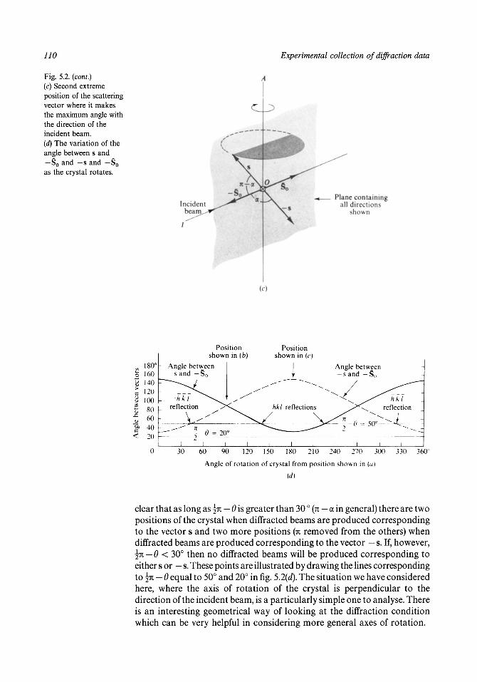
110 Experimental collection of diffraction data
Fig. 5.2. (com)(c) Second extremeposition of the scatteringvector where it makesthe maximum angle withthe direction of theincident beam.(d) The variation of theangle between s and—So and —s and —So
as the crystal rotates.
Plane containingall directions
shown
» 1 8 0°o 160£ 140c »20o 100C 80c 60g> 40•*- *_u
Positionshown in (b)
- Angle betweenL s and - S o
_ hkl ^ S ^ V J ^reflection J^C,^
\ ^ ^ ^ \ ^
- ^ 71
-— --9 = 20°2
1 i i I
Positionshown in (c)
i•
hkl reflections
/ \
i I i
Angle between- s and - §„
/
^ - s - « = 50°-
i i i
_
^ — I^^^^
hklreflection
i
30 60 90 120 150 180 210 240 270 300
Angle of rotation of crystal from position shown in (a)
id)
330 360°
clear that as long as K — 9 is greater than 30 ° (71 — a in general) there are twopositions of the crystal when diffracted beams are produced correspondingto the vector s and two more positions (71 removed from the others) whendiffracted beams are produced corresponding to the vector — s. If, however,71 — 6 < 30° then no diffracted beams will be produced corresponding to
either s or - s. These points are illustrated by drawing the lines correspondingto 71 — 6 equal to 50° and 20° in fig. 5.2(d). The situation we have consideredhere, where the axis of rotation of the crystal is perpendicular to thedirection of the incident beam, is a particularly simple one to analyse. Thereis an interesting geometrical way of looking at the diffraction conditionwhich can be very helpful in considering more general axes of rotation.

5.7 The conditions for diffraction to occur 111
In fig. 5.3,10 represents the direction of the incident beam and a sphere isdrawn which passes through the crystal at 0, has 10 as a diameter and is ofradius 1/L Let us assume that there is a reciprocal-lattice vector s whoseend just touches the sphere at P. Since 10 is a diameter the angle IPO is itand consequently 10P (= (j>) is related to s by
5 = X '
However since s = (2sin0)//l this gives
(5.1)
(5.2)
But when the angle between the incident beam (actually with reverseddirection) and the scattering vector s is rc — 6 a diffracted beam isproduced. The condition for a diffracted beam to be produced is now seento be that the end of the scattering vector s, which is attached to the crystalat O, should just touch the surface of the sphere. The sphere of radius 1/1which is defined above is known as the sphere of reflection or Ewald sphere.One can now follow the process of rotating the crystal about an axis notperpendicular to the incident beam by using the concept of the sphere ofreflection. In fig. 5.4(a) the locus of the end of the vector s as the crystal isrotated is shown and this cuts the sphere at P and Q. When the crystal is insuch a position that the vector s is along OP or OQ a diffracted beam isproduced with indices hkl appropriate to the vector s. The direction of thediffracted beam can also be found from this geometrical construction. In fig.5A(b) a cross-section of the sphere of reflection in the plane IOP is shown.The diffracted beam must be along OD which makes an angle %K — 6 withOP. If C is the centre of the circle then CP equals CO and therefore C^POequals POC and is also equal to POD. Hence CP is parallel to OD andgives the direction of the diffracted beam.
By rotation of the crystal about some axis any diffracted beam can beproduced as long as the end of the scattering vector can be made to lie onthe surface of the sphere. The condition for this is that
Fig. 5.3.The sphere of reflection.When the tip of thevector s touches thesphere the correspondingreflection is produced.
Sphere ofreflection
Incident beamdirection
•

112 Experimental collection of diffraction data
Fig. 5.4.(a) As the crystalrotates the end of thescattering vectortouches the sphere ofreflection at P and Q.{b) CP gives thedirection of thediffracted beam.(c) Neither s nor — scuts the sphere ofreflection as the crystalis rotated.(d) s does not but — sdoes cut the sphere ofreflection as the crystalis rotated.
Sphere ofreflection
Axis of^rotationof crystal
Diffracted beamdirection
ol \7rotation £-"\ ^of crystal
u i
ui)
(5.3)
where 2/1 is the diameter of the sphere of reflection. The sphere of radius 2/2.centred on O within which a vector s must lie in order to satisfy equation(5.3) is known as the limiting sphere.
If a possible reflection is not produced by rotation of the crystal aboutsome particular axis then the situation must be like that shown in fig. 5.4(c).The end of the vector s describes a circular path which does not intersect thesphere. It should be noticed that the reflection corresponding to — s (i.e.hk 7) may not occur (as in fig. 5.4(c)) or may occur (as in fig. 5A(d)).
With these ideas at our disposal we can now consider the various types ofapparatus by which X-ray diffraction data may be collected.
5.2 The powder camera
Frequently it is necessary or convenient to diffract X-rays from a specimenin the form of a fine powder. The powder is usually formed into the shape ofa cylinder either by containing it in a plastic or thin-walled glass containeror by mixing the powder with an adhesive material and shaping it before it

5.2 The powder camera 113
dries hard. Such a specimen will be a myriad of tiny crystallites arranged inrandom orientations. The volume of the individual crystallites in a typicalpowder might be about (5 \imf so that in a specimen of total volume(1 mm)3 the total number of crystallites will be of order 107.
Let us examine what happens when a monochromatic X-ray beam fallson such a specimen. For a particular reflection there will be a large numberof the crystallites in a diffracting position - that is to say, with theirscattering vectors for this reflection making an angle %n — 6 (or very near)with the reversed direction of the incident beam. It should be mentionedhere, anticipating some of the results of the next chapter, that a crystal willreflect over a range of positions near to that corresponding to the Braggangle so that the number of crystallites giving a particular reflection mightbe quite high. Any crystallite giving the reflection will produce a diffractedbeam making an angle 20 with the incident beam and, as is shown in fig. 5.5,the locus of all such diffracted beams is a cone of semi-angle 29 with apex atthe specimen.
Powder cameras vary somewhat in their design but the arrangement ofcomponents for a fairly typical type of camera is shown schematically in fig.5.6(a). A beam of monochromatic X-rays is collimated by passing it througha fine tube (or through a slit system) and falls on the specimen. The film, inthe form of a strip, is contained in a black paper envelope to protect it fromthe light and is wrapped round the inside of the cylindrical camera asshown. The direct beam, which is not diffracted, passes through a hole cut inthe film and is absorbed by a beam trap. This is necessary as otherwise thisradiation would be scattered by the film and fog it over a considerable areathereby obscuring some of the diffraction pattern at low Bragg angles. Thediffraction pattern is recorded by the film as the intersection of cones similarto the one shown in fig. 5.5 with the film. When the film is straightened out itappears as in fig. 5.6(b); this film comes from a camera for which both theincident and straight-through beam pass through holes in the film.
If the powder is fairly coarse so that the crystallites are larger in size andfewer in number then the diffraction lines will not be uniform but tend to berather spotty as in fig. 5.6(c). This can be overcome by rotating the specimenas then many more of the crystallites contribute to each of the diffractionlines. The films shown in fig. 5.6(fo) and fig. 5.6(c) have been taken with andwithout rotation of the specimen, respectively; the improvement in appearanceproduced by rotation is evident.
Frequently the data required by the X-ray crystallographer are a
Fig. 5.5.The locus of thediffracted beams for agiven hkl from all thecrystallites of a powderspecimen.
Diffracted beams fromdifferent crystallites
Direct beam

Motor for roiaiingspecimen
Beam (rap
Film
I(c)
Fig. 5.6.(a) A typical arrangement for a powder photograph.(6) A powder photograph with rotation of the specimen.(c) A powder photograph without rotation of the specimen.

5.2 The powder camera 115
complete set of diffracted intensities together with the correspondingindices of reflection hkl From a powder photograph the only way ofdetermining the indices of a diffraction line, assuming that one knows theunit-cell parameters, is by means of the diffraction angle 29. In fact manydiffracted beams will have similar 26 values (similar magnitudes of s); notonly does this give a problem of identification but, more important still,diffracted beams may overlap completely. If two or more beams fall on topof one another then it is impossible to ascertain the intensities of theindividual components of the composite line and valuable information islost. To get some idea of this problem let us consider how many reflectionsmight be obtained for a crystal structure with a moderate-sized unit cell -say of volume 500 A3. The total volume within the limiting sphere is
and the volume of the reciprocal unit cell will be, from equation (3.26),
K* = (500A3)-\ (5.5)
Thus the number of reciprocal-lattice points within the limiting sphere will be
^=VQV. (5.6)
If the wavelength of the X-rays is that for Cu Ka radiation, 1.54 A, then thetotal number of reciprocal-lattice points equals
/ 2 \ 3
—— x 500=^=4000.1.54y
The number of independent reflections will be lower than this - for examplereflections related by Friedel's law have the same Bragg angle and the sameintensity and always overlap on the powder film. For space groups of highersymmetry there may be fourfold, sixfold or eightfold coincidences ofequivalent reflections but nevertheless it can be seen that for all but thesmallest unit cells the data consist of a large number of independent items.The overlap problem is so severe that powder photographs are normallynot used for the purposes of collecting data for structure determinationunless the alternative of obtaining data from a single crystal is, for somereason, impracticable.
A combination of new needs, new technology and new theory has giventhe powder method a fresh lease of life. Many materials of great potentialtechnological importance, e.g. high-temperature superconductors, maysometimes only be obtained in the form of fine powders. Their powderdiffraction patterns may be collected with a powder diffractometer, aschematic representation of which is shown in fig. 5.7(a). The incident highlymonochromatic X-ray beam is very well collimated which means that theangular spread of the powder lines is reduced as much as possible. Thediffracted radiation is measured by some form of X-ray photon counter (see§ 5.7) with a very fine entrance slit which is slowly rotated about the centralaxis of the instrument. The resultant intensity profile, as shown in fig. 5.7(b),
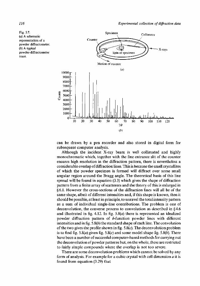
116 Experimental collection of diffraction data
Fig. 5.7.(a) A schematicrepresentation of apowder diffractometer.(b) A typicalpowder-diffractometertrace.
Counter
Specimen\
Collimator
• X-rays
Motion of counter
10000900080007000
2 6000| 5000u 4000
300020001000
0
(a)
uu •J.L .ill 1.110 20 30 40 50 60 70
20
(b)
80 90 100 110 120
can be drawn by a pen recorder and also stored in digital form forsubsequent computer analysis.
Although the incident X-ray beam is well collimated and highlymonochromatic which, together with the fine entrance slit of the counterensures high resolution in the diffraction pattern, there is nevertheless aconsiderable overlap of diffraction lines. This is because the small crystallitesof which the powder specimen is formed will diffract over some smallangular region around the Bragg angle. The theoretical basis of this linespread will be found in equation (3.3) which gives the shape of diffractionpattern from a finite array of scatterers and the theory of this is enlarged in§6.1. However the cross-sections of the diffraction lines will all be of thesame shape, albeit of different intensities and, if this shape is known, then itshould be possible, at least in principle, to unravel the total intensity patternas a sum of individual single-line contributions. The problem is one ofdeconvolution, the converse process to convolution as described in § 4.6and illustrated in fig. 4.12. In fig. 5.8(a) there is represented an idealizedpowder diffraction pattern of ^-function powder lines with differentintensities and in fig. 5.8(&) the standard shape of each line. The convolutionof the two gives the profile shown in fig. 5.8(c). The deconvolution problemis to find fig. 5.8(a) given fig. 5.8(c) and some model shape fig. 5.8(ft). Therehave been a number of successful computer-based methods for carrying outthe deconvolution of powder patterns but, on the whole, these are restrictedto fairly simple compounds where the overlap is not too severe.
There are some deconvolution problems which cannot be solved by anyform of analysis. For example for a cubic crystal with cell dimension a it isfound from equation (3.29) that

5.2 The powder camera 117
Fig. 5.8.(a) An idealizedb -function powderpattern.(b) The shape of anisolated powder line.(c) The actual powderpattern - theconvolution of (a) and
(by
10° 20°
10°20
(c)
20°
4sin20= -Ah2 + k2 n (5.7)
Thus any combinations of Miller indices giving the same values ofh2 + k2 +12 will give exactly overlapping powder lines which no decon-volution process can disentangle. This will occur with pairs of indices[(550), (710)] and [(410), (322)] and the triple of indices [(621), (540), (443)].For a cubic crystal, simple permutations of indices just give equivalentreflections which do not present a problem for powder diffraction analysis.However, in general the number of exactly overlapping powder lines isusually sufficiently small for the crystal structure analysis to be completedwithout using the information from them, although this information can beused subsequently in the process of structure refinement.
An important contribution to the use of powder patterns was made byH. M. Rietveld in 1967 who showed how it was possible to use the wholepattern, including the overlapped lines, to refine crystal structures. Hedescribed a mathematical least-squares procedure (see § 9.4) for refiningatomic positions, thermal vibration parameters (§6.5), lattice parametersand line-profile shapes which are all modified to give the best possible fitwith the observed powder pattern. The number of parameters which couldbe accommodated by this method is of the order of 100, which means that itcan only be applied to comparatively simple structures. Most commercialpowder diffractometers will be provided with a range of software fordeconvoluting the diffraction patterns and also for carrying out Rietveldrefinement.
Powder cameras are often used for the identification of materials. For

118 Experimental collection of diffraction data
example in an industrial process one of the products may be alumina whichcan exist in a number of different forms. It may be necessary to ascertain theform of alumina being produced under different sets of conditions and themost convenient way of doing this is by taking X-ray powder photographs.These can be compared with a set of photographs covering the completerange of forms of alumina and identification would usually be straightforwardand unambiguous.
Powder photographs can also be used to identify completely unknownmaterials. A large number of materials of all types have the major features oftheir X-ray powder patterns listed in a set of ordered cards known as thePowder Diffraction File. The information on one of the cards includes thed-spacings (which can be derived from the Bragg angle by equation (3.37))and relative intensities of the strongest lines of the pattern. The strongestthree lines are displayed at the top of each card and they are listed in theorder of the d-spacings of their strongest lines. The relative intensities ofpowder lines may depend on the shape of the crystallites in the specimenand this may differ from sample to sample. Consequently identification ofmaterials by the Powder Diffraction File is sometimes not straightforwardand requires some patience and ingenuity. If the material to be identified is amixture of two or more materials in unknown proportions then identificationof the components can often be extremely tedious, if not absolutely impossible.
5.3 The oscillation camera
The simplest type of single-crystal camera in common use is the oscillationcamera shown schematically in fig. 5.9. The crystal is glued to a suitable
Fig. 5.9.A typical arrangementfor an oscillation camera.
Film
Collimator— Goniometer
head
Housing for rotatingand oscillating mechanism
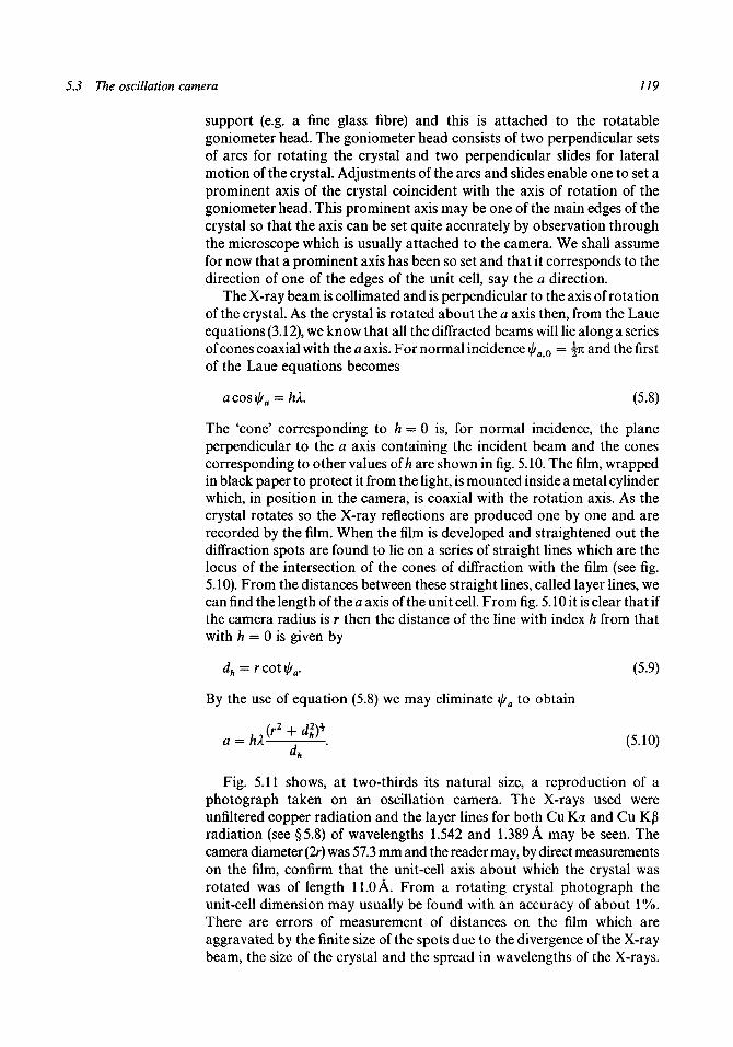
5.3 The oscillation camera 119
support (e.g. a fine glass fibre) and this is attached to the rotatablegoniometer head. The goniometer head consists of two perpendicular setsof arcs for rotating the crystal and two perpendicular slides for lateralmotion of the crystal. Adjustments of the arcs and slides enable one to set aprominent axis of the crystal coincident with the axis of rotation of thegoniometer head. This prominent axis may be one of the main edges of thecrystal so that the axis can be set quite accurately by observation throughthe microscope which is usually attached to the camera. We shall assumefor now that a prominent axis has been so set and that it corresponds to thedirection of one of the edges of the unit cell, say the a direction.
The X-ray beam is collimated and is perpendicular to the axis of rotationof the crystal. As the crystal is rotated about the a axis then, from the Laueequations (3.12), we know that all the diffracted beams will lie along a seriesof cones coaxial with the a axis. For normal incidence \jja 0 = %n and the firstof the Laue equations becomes
acosi//a = hi. (5.8)
The 'cone' corresponding to h — 0 is, for normal incidence, the planeperpendicular to the a axis containing the incident beam and the conescorresponding to other values of h are shown in fig. 5.10. The film, wrappedin black paper to protect it from the light, is mounted inside a metal cylinderwhich, in position in the camera, is coaxial with the rotation axis. As thecrystal rotates so the X-ray reflections are produced one by one and arerecorded by the film. When the film is developed and straightened out thediffraction spots are found to lie on a series of straight lines which are thelocus of the intersection of the cones of diffraction with the film (see fig.5.10). From the distances between these straight lines, called layer lines, wecan find the length of the a axis of the unit cell. From fig. 5.10 it is clear that ifthe camera radius is r then the distance of the line with index h from thatwith h = 0 is given by
By the use of equation (5.8) we may eliminate \jja to obtain
(r2 + dl)*a hV (5.10)
Fig. 5.11 shows, at two-thirds its natural size, a reproduction of aphotograph taken on an oscillation camera. The X-rays used wereunfiltered copper radiation and the layer lines for both Cu Ka and Cu K|3radiation (see §5.8) of wavelengths 1.542 and 1.389 A may be seen. Thecamera diameter (2r) was 57.3 mm and the reader may, by direct measurementson the film, confirm that the unit-cell axis about which the crystal wasrotated was of length 11.0 A. From a rotating crystal photograph theunit-cell dimension may usually be found with an accuracy of about 1%.There are errors of measurement of distances on the film which areaggravated by the finite size of the spots due to the divergence of the X-raybeam, the size of the crystal and the spread in wavelengths of the X-rays.

120 Experimental collection of diffraction data
Fig. 5.10.The diffraction coneswith the incident beamnormal to theoscillation axis which isalso a prominent cell
h = - 4
Fig. 5.11.A typical oscillationphotograph (two-thirdsnatural size).
M • .

5.3 The oscillation camera 121
Fig. 5.12.(a) Location of the zerolayer when the crystalaxis is tilted from therotation axis in avertical planecontaining the incidentbeam.(b) Locus of zero layerin relation to cylindricalfilm.(c) Appearance of zerolayer on the flattenedfilm when the upperpart of the crystal axisis tilted towards theincident beam.(d) Appearance of zerolayer on the flattenedfilm when the lowerpart of the crystal axisis tilted towards theincident beam.
Axis ofrotation
Sphereof reflection
Planeperpendicular
to rotation axis
/ •
Diametralplane containing
incident beam Diffractedbeam
Prominentaxis ofcrystal
Zero layer ofreciprocal lattice
(a) \h\
Changes in the physical dimensions of the films when they are processed arealso important sources of error.
Although the separation of the diffraction data into layers makes thesituation better than for powder photographs there is still nearly alwayssome overlap of diffraction spots. In fact one rarely takes rotationphotographs where the crystal rotates continuously. The cameras areprovided with mechanisms operated by cams which enable one to oscillatethe crystal to-and-fro through a few degrees - 5, 10 or 15° being the usualranges. The cams are so designed that, apart from the inevitable discontinuitiesat the ends of the range, the angular speed is uniform. With a small angle ofoscillation there are many fewer spots on the film and the chances of overlapare thereby much reduced. The photograph in fig. 5.11 is an oscillationphotograph and it will be seen that the spots are all resolved.
Oscillation cameras are rarely used for the collection of intensity databut are sometimes used for the preliminary examination of crystals - thedetermination of unit-cell dimensions and crystal system (see §7.3). Thecrystal can also be accurately set about an axis on an oscillation camera andthen transferred on its goniometer head to one of the more elaboratecameras which are described later. The effect of mis-setting of the crystal in

122 Experimental collection of diffraction data
an oscillation photograph can best be examined by considering two simpletypes of mis-setting; any general mis-setting position can be thought of asbeing compounded of the simple types.
Let us first consider a crystal the prominent axis of which is displaced byan angle s from the axis of rotation in a plane containing the rotation axisand the X-ray beam. This situation is shown in fig. 5.12(a). The sphere ofreflection with centre C is shown, and also the zero layer of the reciprocallattice. Because the axis of rotation is slightly displaced from the crystalaxis, a rotation of the crystal changes the circle of intersection of the zerolayer with the sphere of reflection but, if the oscillation angle is small, wecan, to a first approximation, ignore this change. If P is a reciprocal-latticepoint then a diffracted beam is produced in a direction given by CP. If wetransfer to the actual camera, as in fig. 5.12(ft), the relationship of thezero-layer line to the plane perpendicular to the rotation axis is shown.When the film is opened out and placed so that we are looking at it in thedirection travelled by the incident X-ray beam then the zero layer appearsas in fig. 5.12(c). Such an appearance indicates that the crystal axis is tilted ina fore-and-aft direction such that the top of the crystal is tilted towards theviewer. For a tilt in the opposite sense the appearance of the zero layer isshown in fig. 5.12(d).
The other simple type of mis-setting is when the crystal axis is displacedfrom the rotation axis in a plane perpendicular to the direction of theincident beam. The intersection of the zero layer with the sphere ofreflection is shown for this situation in fig. 5A3(a) and this appears on thecylindrical film as in fig. 5.13(5). The figs. 5.13(c) and (d) show theappearance of the zero layer on the flattened film for both senses of tilt of thecrystal axis, the viewer being taken as looking along the direction of theincident beam. Now in this case the layer line in the central region of the filmis almost straight and makes an angle s with the 'ideal' line corresponding toa perfectly set crystal. This 'ideal' line does not actually appear on the film,although one can usually guess its position to within a degree or so, andtherefore the angle s cannot be directly measured. However if the crystal isrotated through 180° and another oscillation picture is taken about thisnew position then one has gone from situation (c) to situation (d). If bothlayer lines are recorded on the same film and if one, say the first recorded, ismade stronger than the other then the appearance of the film will be asshown in fig. 5.13(e). The angle between the two straight sections of the layerlines is 2s which can be measured easily and the crystal is known to be in theposition corresponding to the second (weaker) layer line.
In practice, in order to set a crystal, one would take the first oscillationpicture with the two arcs along and perpendicular to the direction of theX-ray beam. If the mis-setting has the major characteristics shown in fig.5.13 the two layer lines at 180° separation are recorded and the error insetting is corrected on the arc perpendicular to the beam. If the mis-settinghas the major characteristics of fig. 5.12 then a rotation through %n gives thefig. 5.13 situation and the correction can be made as before. By taking asuccession of photographs and correcting the setting each time the crystalaxis can be set along the rotation axis with a high degree of precision.
The indexing of oscillation photographs can best be done by a graphical

5.5 The oscillation camera 123
Fig. 5.13.(a) Location of the zerolayer when the crystalaxis is tilted from therotation axis in a planeperpendicular to theincident beam.(b) Locus of zero layerin relation to cylindricalfilm.(c) Appearance of zerolayer on the flattenedfilm when the crystalaxis is tilted in ananticlockwise directionas seen looking alongthe direction of theincident beam.(d) Appearance of zerolayer on the flattenedfilm when the crystalaxis is tilted in aclockwise direction asseen looking along thedirection of the incidentbeam.(e) The double zerolayer produced bytaking two oscillationphotographs with thecrystal rotated 180° inbetween.
Axis ofrotation
Sphere ofreflection
Zero layerof reciprocal lattice
Diametral planecontaining incident beam
Planeperpendicular
to rotation axis
Diffractedbeam
beam
Prominentaxis ofcrystal
Zero laver
[a)
Axis of rotation /Axis of rotation
process which will be illustrated for the zero layer. In fig. 5.14(a) there isshown a section of the zero layer of the reciprocal lattice of a crystal situatedat 0 and the diametral plane of the sphere of reflection (the circle ofreflection) which contains the incident beam. As the crystal rotates so doesthe reciprocal lattice and reciprocal-lattice points pass through the circle ofreflection giving diffracted beams as they do so. The relative motion of thecircle and the reciprocal lattice can also be shown by keeping the reciprocal
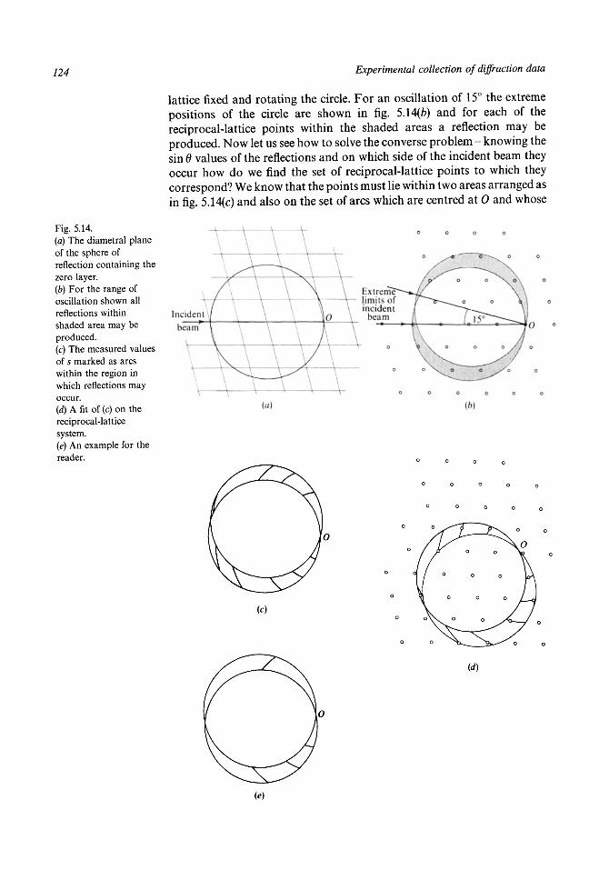
124 Experimental collection of diffraction data
Fig. 5.14.(a) The diametral planeof the sphere ofreflection containing thezero layer.(b) For the range ofoscillation shown allreflections withinshaded area may beproduced.(c) The measured valuesof s marked as arcswithin the region inwhich reflections mayoccur.(d) A fit of (c) on thereciprocal-latticesystem.(e) An example for thereader.
lattice fixed and rotating the circle. For an oscillation of 15° the extremepositions of the circle are shown in fig. 5.14(fc) and for each of thereciprocal-lattice points within the shaded areas a reflection may beproduced. Now let us see how to solve the converse problem - knowing thesin 6 values of the reflections and on which side of the incident beam theyoccur how do we find the set of reciprocal-lattice points to which theycorrespond? We know that the points must lie within two areas arranged asin fig. 5.14(c) and also on the set of arcs which are centred at 0 and whose
Incidentbeam
Extreme- limits of
incident0 \ beam
[a]
(c)
(e)

5.4 The Weissenberg camera 125
distances, at the scale of the reciprocal lattice, correspond to the sin 8 valuesof the observed reflections. If a transparent replica of fig. 5.14(c) is placedwith O over the origin of a reciprocal-lattice net and is pivoted about O aposition will be found when each of the sections of arc passes through areciprocal-lattice point. Such a fit of arcs to points (not all perfect because oferrors of measurement) is shown in fig. 5A4(d). The reader may try forhimself the problem of fitting the arcs in fig. 5.14(e) on to the same net.Similar considerations apply to the indexing of non-zero layers althoughthis introduces some additional complications.
If the principles of the oscillation camera have been dealt with in somedetail it is because it is a simple camera, not difficult to understand, in whichone can readily see the basic principles of X-ray diffraction from crystals. Inaddition it will have demonstrated how useful is the concept of thereciprocal lattice in interpreting the results which one obtains.
5.4 The Weissenberg camera
While it is quite feasible to collect complete sets of X-ray intensity data withan oscillation camera the inconvenience of indexing the photographs issuch that they are hardly ever used for this purpose. We shall now examinea more convenient instrument, the Weissenberg camera, which makes thetask of indexing photographs quite straightforward and which also enablesa whole layer of information to be collected at one time without overlapdifficulty.
In fig. 5.15(a) there is shown a crystal mounted on a goniometer headwith an X-ray beam incident normal to the axis of rotation. There are also
Fig. 5.15.{a) Layer-line screensset for the zero layer.(b) Layer-line screensset for an upper layer.
Incident beam
Layer-line screens1 \
Incident beam

126 Experimental collection of diffraction data
shown a pair of cylindrical metal screens which can be adjusted so that acircular slit occurs between them and this slit can be so arranged that oneand only one of the layer lines passes through it. Diffracted beams in otherlayer lines will strike the screens and be absorbed. In fig. 515(a) the screensare adjusted to let through the zero layer and in fig. 5.15(b) a higher layer isallowed through.
A film, inserted into a cylinder and placed coaxial with the screens willrecord only a single layer but, if the crystal is completely rotated, there willbe overlap of spots for diffracted beams which pass through the same pointsof the slit (same values of Bragg angle). It should be recalled that thediffracted beams occur wherever a reciprocal-lattice point passes throughthe sphere of reflection and although two reflections may have the sameBragg angle they will not be produced at the same time. In the Weissenbergcamera the crystal is oscillated, the range of the oscillation being under thecontrol of the user and may be greater than 180°. The film holder can movealong the direction of its axis, which is also the axis of oscillation, and it ismechanically coupled to the rotation of the crystal in such a way that itslides backwards and forwards as the crystal oscillates to-and-fro. Asuccession of positions through one cycle of the motion is shown in fig. 5.16.Wherever the crystal passes through a position for a particular reflection tooccur the film is always in the same relative position and the diffracted beamstrikes the same point of the film. The general effect of the film motion is tospread the data in a single layer over the whole area of the film and nooverlap of spots can possibly occur. If spots are produced at different timesthen they will be displaced from one another along the direction of themotion of the film.
The distance travelled by the film holder is linearly related to the angle ofrotation of the crystal. Let us consider fig. 5.11 (a) which represents thediametral plane of the sphere of reflection containing the incident beam.The reciprocal-lattice point P is in the zero layer and has coordinatesrelative to O of (s, </>). The crystal and the film are at one of the extremepositions of their periodic motions and we wish to determine where on thefilm the diffracted spot will fall. The film in a Weissenberg camera can eitherbe mounted in two halves or can be in one piece with a beam stop attachedto the collimator and inside the layer-line screens (fig. 5.17(fo)). In fig. 5.17(c)we are shown one-half of the film with the location of the slit indicated andalso the line corresponding to 6 = 0. The point Q may be taken as the originof a Cartesian coordinate system. The coordinate parallel to the slit isproportional to 20, the angle of diffraction and we may write
y = 2rO (5.11)
where r is the radius of the film cylinder. The x coordinate, which measuresthe distance travelled by the film, is proportional to the angle throughwhich the crystal rotates, say if/, and we may write
x = kij/. (5.12)
Some typical values of these constants are 2r = 57.3 mm (note there are 57.3angular degrees per radian) and k = 0.5 mm/angular degree.
Turning back to fig. 5.17(a) we can see that the reflection will be
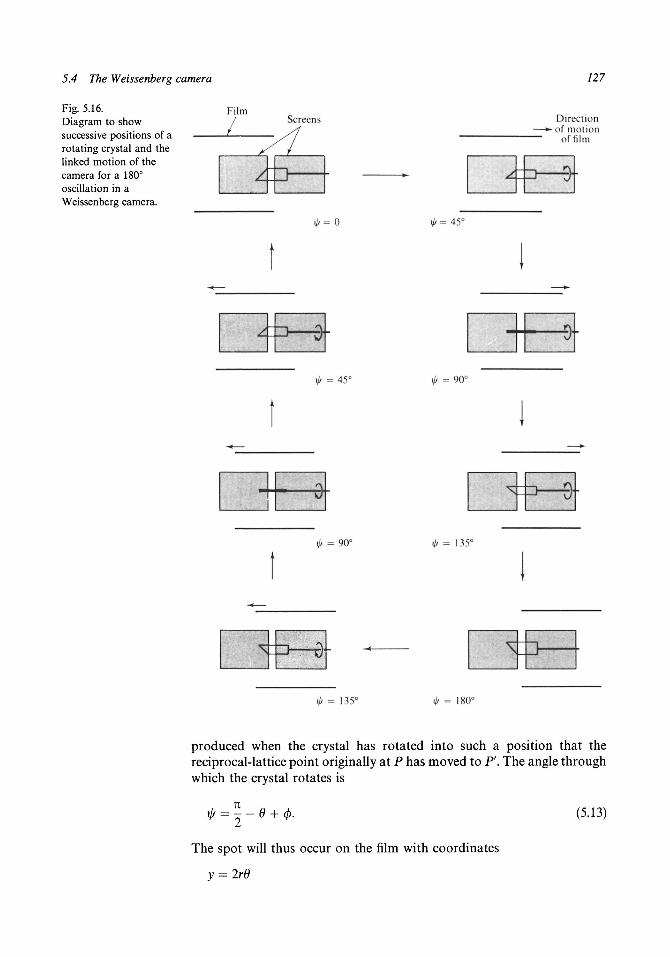
5.4 The Weissenberg camera 127
Fig. 5.16.Diagram to showsuccessive positions of arotating crystal and thelinked motion of thecamera for a 180°oscillation in aWeissenberg camera.
FilmScreens
\j/= 0 \f/= 45°
Direction- of motion
of film
= 45° = 90°
-o-
»// = 90° - 135°
5
- 135° = 180°
produced when the crystal has rotated into such a position that thereciprocal-lattice point originally at P has moved to Pf. The angle throughwhich the crystal rotates is
: 2(5.13)
The spot will thus occur on the film with coordinates

128
Fig. 5.17.(a) The reflectioncorresponding to thepoint P occurs when ithas rotated to point F.(b) The arrangement offilm in a Weissenbergcamera.(c) A row ofreciprocal-lattice pointscollinear with theorigin.
Experimental collection of diffraction data
Film
Back stop
[a]
Line of centreof slit
0 = 0
Incidentbeam
Line ofx centre
of gap
Incidentbeam
Collimaior
tb)
Row of reciprocallattice spots
(c) id]
(5.14)
Suppose that we have in the zero layer a line of reciprocal-lattice pointscollinear with the origin which might, for example, be one of the prime axeswe select for the reciprocal lattice. Such a row of spots is shown in fig. 5.17( d)together with the section of the sphere of reflection. For all these points 0has the same value and from the two equations (5.14) we find, eliminating 6,that
y = —— x + r(n (5.15)
This is the locus of the reciprocal lattice points on the film, as shown by thediffraction spots, and, since (j) is constant, it is a straight line. The slope ofthis line, — 2r/k, is a function of the design constants of the camera.
A Weissenberg picture may be regarded as a distorted projection of thereciprocal lattice. In fig. 5.18(<z) there is shown a representation of a polarcoordinate grid in reciprocal-lattice space. The angular coordinate 0 ismeasured from some arbitrary origin and the radial coordinate s is themagnitude of the normal reciprocal-lattice vector. The corresponding gridin Weissenberg space is shown in fig. 5.18(£). The lines of constant <j> at equalincrements of <j> appear as a set of equidistant, parallel straight lines of slope— 2r/k. Since s is proportional to sin 9 and the y coordinate is proportionalto 8 (see equation (5.11)) the lines of constant s at constant increments of 5 inWeissenberg space are parallel but not equidistant. The two thicker lines in

<t> = 9 0 °
180°
Circles at 0.2 IXincrements of s <t> = o
As = 2.0
7 /////////////i n / / / / / / / / / / / 7 7
0 8 / / / / / / / / / / 1 / 77 / / / / / /7777 //////// / t i l
/ / / I0 8?/ /p/ / / / / / 7777
7 / / / / / / / / / / 7 /
(b)
- 180° (f> = 270° <f) = 360°
= 180°
= 0 = 90° </> = 180°
1.8
1.61.41.21.00.80.60.40.20.0.0.20.40.60.8
(c) 1.01.21.4
1.6
1.8
//
//
/
//' /
1/
//
///
1/
/
L L
////7w///,//////// / /// / // / / / // / / // / / / // / / / // / / / ./ / / / /' / / / // / / / /
< • / / / /
/ / / / ,
/ / / 1 /J-LLL' / /
/ / / • :
%
/ / ,
/ // / /
/ /
/ / ,/ /
/ // /
/ /f / I
/ /
/ /
' 1 // /1 / ;/ /
/ // :I
t(
/ 1
1
I
/
1
7f/
/
//
/i
/
/ / // / / /
/ / // / / /
/ / // / / /
f / / // /
/ / / // • i
/ / / // / /
/ 1 1 // / /
/
2.06 - 360°
Fig. 5.18.(a) The diametral plane of the sphere of reflection containing the incident beam marked with a polar-coordinate system.(b) The transformation of the grid shown in (a) in Weissenberg space. (Half-scale for 2r = 57.3 mm, k = 0.5 mm/angular degree.)(c) The transformed grid within a region which could occur on a Weissenberg film. (Half-scale for 2r = 57.3 mm, k = 0.5 mm/angular degree.)
<t> = 270° = 180°

130 Experimental collection of diffraction data
fig. 5.18(fc) correspond to the complete line (j) = 0° plus (j> = 180° in fig.5.18(a). It should be noticed that the arrangement of slits and film move-ment for the Weissenberg camera results in the diffraction spots falling on arectangular area of the film. The points P and F are equivalent and therectangular area shown in fig. 5.18(c) is equivalent to that shown in fig. 5.18(fe).
It is possible to find the locus in Weissenberg space of a set of linesparallel to the thicker one in fig. 5.18(a); such a set of lines is shown in fig.5.19(a) contained within the limiting circle of radius 2/1 The spacing of thelines is 0.1 of the radius of the limiting circle and when they are plotted inWeissenberg space they appear as shown in fig. 5.19(b). The derivation ofthe precise form of these curves is fairly straightforward but we shall notderive them here. Now let us suppose that in the zero layer of the reciprocallattice we draw two sets of parallel lines within the limiting circle as is shownin fig. 5.20(a). In Weissenberg space these will appear as in fig. 5.20(b); thereader should study this figure for a short time to see the relationshipbetween the reciprocal-space diagram and that in Weissenberg space. Theintersections of the sets of lines in fig. 5.20(a) could be regarded as zero-layerreciprocal-lattice points with each of which there is an associated intensityand the Weissenberg diagram would give a diffracted spot at each cor-responding point. The lines of the grid are shown in fig. 5.20(fr) and these arelabelled with indices h and k. It is normally fairly easy to see the families ofcurves on which the spots lie and therefore to index the reflections. Theactual Weissenberg photograph shown in fig. 5.20(c) may be compared tofig. 5.20(fe).
In the arrangement shown in fig. 5.15 the incident X-ray beam is normalto the rotation axis for all the layer lines. It is more usual to use the'equi-inclination method' for taking upper-layer photographs. The incidentX-ray beam and the diffracted beam make the same angle with the rotationaxis as illustrated in fig. 5.21; the angle \i between the incident beam and theaxis is, from equation (3.12), given by
2a cos [i = hX. (5.16)
It should be noted that the angles corresponding to x//a0 and ij/a in equation(3.12) are n — jn and fi, respectively.
The equi-inclination method has the advantage that the family of curvescorresponding to parallel lines in a reciprocal-lattice layer have the sameshape regardless of which layer is taken and, by applying scaling factors,one chart showing these curves can be used for all layers. The detailedtheory of equi-inclination Weissenberg diagrams for upper layers is to befound in X-ray Crystallography by M. J. Buerger (Wiley).
5.5 The precession camera
The Weissenberg camera gives a distorted map of a reciprocal-lattice layerwhich, as we have seen, can be translated back to the actual reciprocal-latticelayer by means of standard charts. Usually this operation presents littledifficulty but, sometimes, particularly when the unit cell has one or morelong axes, this process can lead to errors. If a number of adjacent spots aretoo weak to be seen in an otherwise highly populated row corresponding to

Parallel lines atspacing 0.2/A
Limitingcircle
Fig. 5.19.(a) A set of equidistant parallel lines in the diametral plane of the sphere of reflection.(b) The transformation of {a) in Weissenberg space. (Half-scale for 2r = 57.3 mm, k = 0.5 mm/angular degree.)

132 Experimental collection of diffraction data
Fig. 5.20.(a) Two sets ofequidistant parallel linesin the diametral plane ofthe sphere of reflection.(b) Part of thetransformation of (a) inWeissenberg space.(Half-scale for2 r = 57.3 mm,k = 0.5 mm/angulardegree.)
8 6 4 2 0 2 4 6 8 1012 14I I I I I I I I I I I I i I I I I ! I I I i I I I I I I I
0=88.5°
</> = 1 8 0 ° " "--
...
.J. . . . . .
. "4-4-1
— 12- 1 0
— 6
-- f - 4
26 = 0 ° -
0=268.5°
(a)
-0k
A = 12
(b)
a line of reciprocal-lattice points then it is possible to mis-index thehigher-order reflections. This can be caused by very slight mis-positioningof the Weissenberg chart on the photograph; although such errors can beavoided by very careful measurement on the photograph this can be atedious process. In such a case it would be an advantage to have a camerawhich would give an undistorted map of the reciprocal lattice. The locationof a spot in relation to its fellows may then be determined by a straight edgealone and the possibility of error is much reduced. However even when theunit-cell edges are all of moderate dimensions, it is convenient to obtaindirectly an undistorted picture of the reciprocal lattice.

5.5 The precession camera 133
Fig. 5.20 (cont.)(c) A Weissenberg filmcorresponding to thelattice shown in (b). Onlyone-half of the film isshown. Natural size.
Fig. 5.21.The equi-inclinationarrangement for higherlayer Weissenbergphotographs. Theincident and diffractedbeams make angles7i — \i and n,
respectively, with therotation axis.
Incidentbeam
Diffractedbeam
Conical surfaceon which lie all
diffracted beamsof this layer line
Axis of rotationof crystal
It was shown by de Jong and Bouman (1938) that a camera could bedesigned which would represent without distortion a layer of the reciprocallattice. We shall examine here a special case of the de Jong and Boumanarrangement- one which is simple to understand and illustrates the generalprinciples of the method.
In fig. 5.22(a) there is represented a crystal at C with an incident X-raybeam normal to a prominent cell axis whose direction is CD. The sphere ofreflection is shown and also the intersection of the sphere by an upper layer,say the nth, of the reciprocal lattice. If any reciprocal-lattice point lies onthis ring of intersection, say at F, then the corresponding X-ray reflection isproduced. If 0 is the centre of the sphere then the direction of the diffracted

134 Experimental collection of diffraction data
Circle of intersectionof nth layer and
sphere of re flee [ion\
t Axis of rotation
C
Region of mh layer D i f f r a c l e d
which can be recorded
Axis of rotation
. Diffracted beam
Incident
Sphere ofreflection
Incident beam \yLayer-line
screen
0( rystal
ib)
^ Axis of Axis of rotation of filmCJS> rotation
Cross section ofsphere of re flee I ion
of crystalFilm
* Layer-line screen
Fig. 5.22.{a) The intersection ofthe nth layer of thereciprocal lattice withthe sphere of reflection.The accessible area ofthe nth layer is theannular region shownshaded.(b) A layer-line screenarranged to allowthrough only the nthlayer.(c) If the film is rotatedabout C" with the sameangular velocity as thecrystal an undistortedprojection of thereciprocal-lattice sectionis produced.
beam is given by OP. If the crystal is rotated about its prominent axis thenthe reciprocal lattice, with its origin at the point C, rotates about CD; as itdoes so the nth layer slices through the sphere of reflection cutting it in thering shown. Whenever a reciprocal-lattice point lies on the circle ofintersection, which it will do twice on each revolution, a diffracted beam isproduced along the direction joining 0 to the reciprocal-lattice point. Ithelps to visualize the situation if we imagine the crystal actually located at 0rotating about the line OE while the reciprocal lattice is displaced from itwith its origin at C and rotating about CD with the same angular velocity asdoes the crystal. The reciprocal-lattice layer would rotate about the pointC in its own plane and one could record data corresponding to latticepoints within the annular region shaded in the figure.
With the arrangement described all the diffracted beams from the nthlayer would lie on the surface of a cone with apex 0 and if a flat piece of filmwas placed perpendicular to OE then the separate layers would appear asrings of spots on the film, each ring being the intersection of the appropriateconical surface with the plane of the film. It is possible to separate one layerline by interposing in the path of the X-rays a metal screen with an annularslit cut into it. The central ring of metal is kept in place by fine cellophane orplastic film which is almost completely transparent to X-rays. The relationshipof this layer-line screen to the crystal and incident beam is shown in fig. 522(b).
The de Jong and Bouman method, like the Weissenberg method, spreadsout the record of the diffraction data by moving the film. The way in which

5.6 The photographic measurement of intensities 135
this is done may be followed by reference to fig. 5.22(c) which shows across-sectional view in the plane of the sphere of reflection containing theincident beam. The point C" is the projection from 0 of the point C on tothe plane of the film. If the film is rotated about an axis through C" parallelto CD at the same angular velocity as the reciprocal lattice then the linejoining O to any reciprocal-lattice point in the nth layer always intersectsthe same point on the film. Thus whenever a particular reciprocal-latticepoint passes through the circle of intersection the diffracted beam strikesthe same place on the film. The exposed points on the film are thus aprojection of the reciprocal-lattice layer from the point O on to the plane ofthe film and the developed film will show a true undistorted picture of thereciprocal-lattice layer.
It will be noticed that the experimental arrangement which has beendescribed is incapable of giving the zero-layer data and also presentsconsiderable mechanical difficulties for layers close to the zero layer. Manyother experimental arrangements are possible and their various advantagesand disadvantages have been discussed by Buerger (loc. cit). In fact thecamera which is most frequently used to record diffraction data on anundistorted reciprocal-lattice net is the Buerger precession camera. Thisenables all layers to be recorded and for the layers to all be on the samescale. A typical film produced by a precession camera is shown in fig. 5.23.We shall not attempt to describe the complexities of the precession camerahere; for our purpose a description of the de Jong and Bouman arrangementsuffices to explain the basic theory of methods of this type.
For a given wavelength the precession camera records less of reciprocalspace than does the oscillation or Weissenberg camera and therein lies itschief disadvantage. However, as will be clear from fig. 5.23, it enablesangular measurements to be made more easily.
5.6 The photographic measurement of intensities
X-ray crystallographers have relied and, to some extent, still do rely on thephotographic recording of diffraction data. Before very fast films wereavailable it was customary to use an intensifying screen. This was a layer offluorescent material placed behind the film in such a way that the X-rayspassed through the film and then hit the screen. The bulk of the exposure ofthe film was caused by the photons of visible light released by the screenrather than by the direct X-ray beam itself. However, such screens are rarelyused now; fast films, very sensitive to X-rays, are used and these arenormally double-coated, that is covered with sensitive emulsion on bothsides, to increase their sensitivity still further.
Usually one does not try to measure the intensities of the reflections byan absolute method. If the spots on the film are similar to one another inappearance then one can produce an intensity scale by exposing onereflection along a strip of film for various lengths of time with the X-ray tuberunning under constant conditions. The relative intensities of the diffractionspots can then be determined by comparison with the scale. The eye is verygood at comparing intensities for spots in the intermediate range of densitybut is less efficient for spots which are either very faint or very dense.

136
Fig. 5.23.A typical photographfrom a precessioncamera.
Experimental collection of diffraction data
It is frequently found that the recorded diffraction spots are not all ofsimilar appearance and then it is not the intensities of the spots we wish tomeasure but the total energies of the X-ray beams which have producedthem. X-ray crystallographers are guilty of lax terminology here and use theword 'intensity' to denote total energy, since the total energy is proportionalto the quantity Jhkl in equation (3.43). We shall use the term 'energy' todenote the total energy of the diffracted beam.
The reasons for the variation in spot appearances are manifold. Forinstance, the spots tend to become more diffuse at higher Bragg angles dueto the finite bandwidth of the X-ray spectral lines. From Bragg's law,equation (337), by differentiation and rearrangement, we find
d9 =Id cos 9
(5.17)
and since cos 9 decreases as 9 increases so the diffraction image becomesmore diffuse for high 9. This effect may be seen in fig. 5.20(c) where at highBragg angles the Kax and Ka2 wavelengths (see §5.8) produce resolvablediffraction spots.
However a more important reason for the spread of diffraction spots is
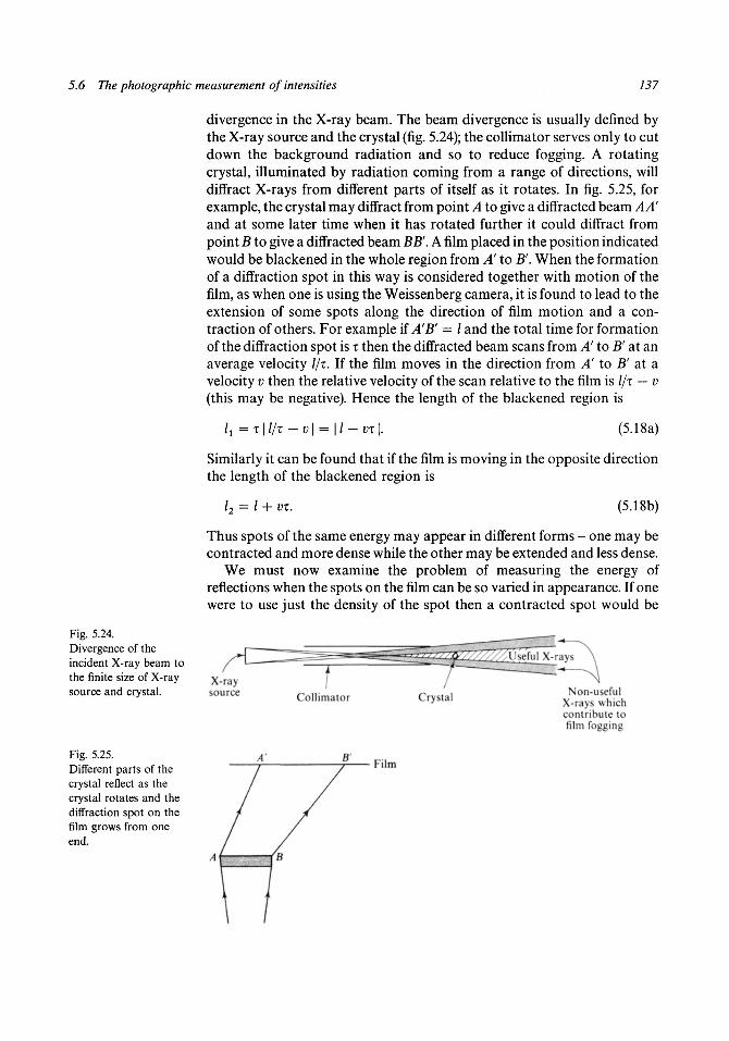
5.6 The photographic measurement of intensities 137
Fig. 5.24.Divergence of theincident X-ray beam tothe finite size of X-raysource and crystal.
Fig. 5.25.Different parts of thecrystal reflect as thecrystal rotates and thediffraction spot on thefilm grows from oneend.
divergence in the X-ray beam. The beam divergence is usually defined bythe X-ray source and the crystal (fig. 5.24); the collimator serves only to cutdown the background radiation and so to reduce fogging. A rotatingcrystal, illuminated by radiation coming from a range of directions, willdiffract X-rays from different parts of itself as it rotates. In fig. 5.25, forexample, the crystal may diffract from point A to give a diffracted beam AAr
and at some later time when it has rotated further it could diffract frompoint B to give a diffracted beam BB'. A film placed in the position indicatedwould be blackened in the whole region from A' to B'. When the formationof a diffraction spot in this way is considered together with motion of thefilm, as when one is using the Weissenberg camera, it is found to lead to theextension of some spots along the direction of film motion and a con-traction of others. For example if A'B' = / and the total time for formationof the diffraction spot is T then the diffracted beam scans from A' to B' at anaverage velocity //T. If the film moves in the direction from A to B' at avelocity v then the relative velocity of the scan relative to the film is //T — v(this may be negative). Hence the length of the blackened region is
lx =T\l/T -v\ = \l-vx\. (5.18a)
Similarly it can be found that if the film is moving in the opposite directionthe length of the blackened region is
/ - / + vx. (5.18b)
Thus spots of the same energy may appear in different forms - one may becontracted and more dense while the other may be extended and less dense.
We must now examine the problem of measuring the energy ofreflections when the spots on the film can be so varied in appearance. If onewere to use just the density of the spot then a contracted spot would be
Useful X-rays
: * ~N on-useful
X-rays whichconiribute tofilm fogging
X-raysource Collimator
B
Crystal
Film

138 Experimental collection of diffraction data
Fig. 5.26.A typical curve ofdensity vs log(exposure) for an X-rayfilm.
judged as more intense than an extended one. The quantity one is reallytrying to measure is the total energy T of the radiation producing the spotor, what amounts to the same thing, the total number of photons falling onthat region of the film. Film obeys the so-called reciprocity law, that is to saythat the effect on the film is proportional to the total exposure E asmeasured by the product of beam intensity and time. Since intensity is ameasure of energy per unit area per unit time then £ is a measure of energyper unit area. The quantity we wish to determine is then given by
T= \EdA (5.19)
where the integration is over the whole area of the diffraction spot.The blackening of a photographic emulsion is measured by its density
defined by
110 fractional transmission of light'
(5.20)
Thus if a certain region of a film transmits 1 % of incident light then, for thatpart of the film, D = 2. The behaviour of films on exposure to radiationdepends on the wavelength of the radiation and also very critically on thedeveloping process. However the general character, expressed as a relationshipbetween D and E, usually resembles that shown in fig. 5.26. The fog levelmay vary a great deal and depend on the duration and temperature ofstorage of the film, the cleanliness of the developing and fixing solutions andalso exposure to ambient cosmic radiation before use. Fast films areparticularly prone to a high fog level. Ideally when comparing diffractionspots with an intensity scale it is better to be in the range of £ correspondingto the steepest part of the curve for it is in this region that small differences ofE can most readily be detected by eye. However the quantity E will varyfrom point to point of a given spot and when the spots are all of differentareas it is not easy to assess the relative values of T defined in equation(5.19). There is no simple photometric method whereby measuring theattenuation of a beam of light passing through the whole spot gives areasonable measure of T. It is possible to scan the diffraction spot with a fine
3.0
2.0
1.0
Fog level
log£

5.6 The photographic measurement of intensities 139
beam of light, to determine D (and hence E from the known D-Erelationship) at the points of a grid covering the spot and hence to find Tona relative scale from the sum E£.
For accurate photographic work, one would normally use an integratingmechanism either with a Weissenberg or a precession camera. This is adevice which, at the end of every cycle of operations of the camera, movesthe film in such a way that consecutive images of the same diffraction spotfall on the film with displacements corresponding to the points of a smallrectangular grid. This is illustrated in fig. 5.27 where 25 images of the singlediffraction spot shown in (a) are represented with displacements on a 5 x 5grid in (b). The multiple image will have a flat plateau at its centre thedensity of which will correspond to a total exposure proportional to T. Thepoint P in (b) for example has been subjected to exposures from each of theimages and these exposures come from points similar to those shown in thegrid in (a). Thus the total exposure at P is H£ where the sum is over thepoints of the grid and, since this summation is, to a first approximation,proportional to the integral in equation (5.19), it will be proportional to TThe usual practice is to compare the densities of the plateaux with a scalethe elements of which are small uniform spots made by exposure to thedirect X-ray beam through a circular aperture.
There is shown in fig. 5.28 a Weissenberg picture, normal on one half andintegrated on the other. Quite high precision can be reached by themechanical-integration method. Because of the spreading out of thediffraction data longer exposures are required and weak spots may bemissed altogether. However the very weak spots can be measured onnon-integrated photographs and related to the integrated data by comparisonwith stronger spots with similar shapes.
Automatic densitometers are available which enable rapid and quiteaccurate assessments to be made of the quantity Tin equation (5.19). Onesuch instrument, computer-controlled, scans the spots with a small sourceof light produced on the screen of a cathode-ray tube, the transmitted lightbeing measured by a sensitive photocell. The background round the spot isalso measured and the integral in equation (5.19) is then computed auto-matically. Once the film has been taken the actual measurements can bemade at about one spot per second or even faster.
Fig. 5.27.The superposition ofseveral images of thediffraction spot on a filmto produce a uniformplateau of intensity atthe centre.
[a) (b)

140
Fig. 5.28.A Weissenberg filmshowing unintegratedspots on the right-handside and integrated spotson the left-hand side.
Experimental collection of diffraction data
5.7 Diffractometers
The energy of diffracted beams can also be measured by a counting devicewhich records individual X-ray photons. The Geiger-Muller counter hasbeen used for this purpose and fig. 5.29 shows a schematic G-M counter.The cathode is a metallic cylinder and the anode a wire along the axis of thecylindrical glass envelope. A potential is maintained between the electrodes,of the order of 1000 volts, such that a discharge does just not take place butso that the apparatus is in a critical condition. A single X-ray photon fallingon the gas in the tube can produce primary ions which in their turn producea cascade of secondary ions and a discharge through the counter. Thisdischarge can be detected electronically and amplified to operate arecording instrument. After each discharge the counter must be quenched -that is to say, the residual ions in the tube must be removed. This can beachieved by having an organic vapour in the tube - methylene bromide iseffective - the molecules of which absorb ions and dissociate rather thanproduce fresh ions.
The time for a G-M counter to restore its initial condition afterdischarging is called the 'dead time' of the counter and is typically of theorder 10 " 4 seconds. In practice up to about 3000 photons per second can becounted with a G-M counter. At the higher counting rates proportionalitybetween photon flux and counter discharges is lost because of the increasing

5.7 Diffractometers
Fig. 5.29. Cylindrical cathodeA schematic [_Geiger-Muller counter.
Amplifier
TAnodeGlass envelope
probability that photons will arrive in the dead time when they cannot becounted.
Another type of counter is the proportional counter. This is similar to aG-M counter but operates below the Geiger threshold. Consequently thevoltage pulses produced are small (~ 1 mV) and require amplification.
An X-ray photon entering the counter produces a pulse of heightproportional to the energy of the X-ray photon. This has the advantage thatpulses due to unwanted photons (e.g. second-order reflections with wave-length A/2) can be recognized and eliminated.
Proportional counters also have the advantage of a short dead time(~ 10~7s) and so give a linear response at high counting rates.
Discharge counters have largely been superseded by the scintillationcounter where the radiation first falls on a fluorescent material the visiblelight from which is subsequently detected by a photomultiplier arrangement.In fig. 5.30 a typical set-up is illustrated. The photon of visible light first fallson a photoemissive surface which generates a photoelectron. The layers of'venetian-blind' electrodes are each at about 100 volts higher potential thanthe one before. Each time an electron collides with an electrode it isenergetic enough to produce several secondary electrons each of which isaccelerated in the field to the next electrode and produces several more.This cascade effect can give a millionfold or more amplification factor andthe final pulse of current can be amplified electronically and fed into acounting system. If a high-frequency electronic system is used the scintillationcounter is capable of counting of the order of 107 to 108 events per second.This is so much greater than the rate at which X-ray photons would arrivein a diffracted beam that the scintillation counter gives a count proportionalto the total energy of the beam - that is to say, that the probability of twoX-ray photons arriving so close together that they cannot be countedseparately becomes vanishingly small.
It is possible to incorporate a counter in a diffraction instrument basedon any of the geometrical arrangements we have previously considered. Thecrystal can be placed in a diffracting position, the counter placed so as toreceive the diffracted ray and the counting rate will then be a direct measureof the power of the beam. Devices incorporating counters, rather thantaking a photographic record, are called diffractometers and, in § 5.2, wehave already mentioned a powder diffractometer which records with acounter rather than film.
A typical fully-automatic four-circle diffractometer is shown schematically

142 Experimental collection of diffraction data
Fig. 5.30.A schematic view of ascintillationcounter-photomultiplierarrangement.
ScintillatorPhotosensitive
cathode
—_ Electron paths
\
10-12 layers of'venetian-blind'
electrodes
Anode
in fig. 5.31. The term 'four-circle' refers to the number of rotational motionsavailable and in the instrument shown three of these are associated with thecrystal and one with the counter. The counter rotates about a vertical axisso that the plane containing the incident and diffracted beam is alwayshorizontal. For a particular reflection the counter is set at a positioncorresponding to the Bragg angle; the rotation axis corresponding to thismotion is called the 20 axis. Once this has been done the diffracted beam canbe produced by positioning the crystal so that the scattering vector s makesthe correct angle with the incident and diffracted beams. Such positioningcan be achieved by rotation of the crystal about the three axes shown in fig.5.31 - the <j), x and Q. axes.
Modern single-crystal diffractometers are computer-controlled and areprovided with sophisticated software to carry out many tasks. They canautomatically determine the orientation of the crystal, move the crystal anddetector to record each diffracted beam and also control the time each beamis measured to optimize the accuracy of the measurements. Using the storedintensity data the computer can then solve the crystal structure, usually bymeans of a so-called direct method as described in §8.8.
The accuracy which can be obtained with diffractometers depends on anumber of factors. It is important that the X-ray tube output should be keptabsolutely constant with time as the data is collected. This requires astabilized power supply for the tube but in addition one should monitor areference reflection from time to time to ensure that there is no variation inthe intensity of the incident X-ray beam. Another possible source of error isthe statistical fluctuations which are to be expected in the diffracted beam. Ifin a given time t, N counts are made then the standard error in the numberof counts is y/N. This means that, from normal statistics, there is a 68%probability that the 'true' number of counts is in the range N ± y/N, a 95%probability that it is in the range N ± 2y/N and a 99.7% chance of it beingin the range N ± 3^/iV. By the 'true' number we mean the average numberof counts per unit time, as ascertained by counting for an infinite period,multiplied by t; we should note that this 'true' number is not available to us

5.8 X-ray sources 143
Fig. 5.31.A typical four-circlediffractometer. Thecounter rotates aboutthe 20 axis in one planeand the crystal may beorientated in any wayby the three axes ofrotation (j>, x a n d ^ .
20 Rotation
- only the number N. The diffracted beam power will thus be proportionalto N/t with a fractional standard error
N
N(5.21)
Thus to have a standard error of 1% we must make 10000 counts, for0.1% we need 106 counts and so on. The number of counts which can bemade is clearly limited by the time available to collect the data. It is alsoobvious that for weak reflections one must count over a considerable periodof time to get reasonable accuracy. A typical count rate for a strongreflection would be about 30000 counts per second, while a weak butobservable reflection could give a count rate of 3-10 counts per second. Adisturbing influence, especially for the weak reflections, is the inevitablebackground count; it acts as a noise in the presence of which the signal mustbe measured. However, whatever the difficulties with the use of diffractometers,they are potentially the most accurate and certainly a very convenientmeans of collecting diffraction data. For the study of the crystal structure oflarge biological molecules, where hundreds of thousands of items of datamust be collected, diffractometers, or automatic densitometers, makepossible what otherwise would border on the impossible.
A complete account of the use of diffractometers is given in SingleCrystal Diffractometry by U. W. Arndt and B. M. T. Willis (CambridgeUniversity Press).
5.8 X-ray sources
Over the years the most important source for the production of X-rays forthe crystallographic community has been the sealed hot-cathode tube. Inthis device, illustrated in fig. 5.32, electrons from a heated filament areaccelerated through a potential difference V towards an anode on whichthere is a disk of tarket material - copper, molybdenum, cobalt or some

144 Experimental collection of diffraction data
Fig. 5.32.A sealed hot-cathodeX-ray tube. X-rays fromthe line source areviewed obliquelythrough the berylliumwindows so forming aneffectively compactsource.
Waterout
X-rays
Beryllium window
X-rays
Heated filament
Evacuatedenclosure
other metal. Some of the energy lost by the electrons on striking the target isconverted into electromagnetic radiation in the form of X-rays and, if theaccelerating potential V is sufficiently low, then there will just be acontinuous intensity distribution of X-rays as shown in fig. 5.33(a). Thelower limit of X-ray wavelength 2min, indicating the most energetic X-raysproduced, will have energy corresponding to all the energy of one electron,eV, going into a single X-ray photon. If the accelerating potential isincreased then eventually a point will be reached where the impactingelectrons can eject inner core electrons from the target element. At thispoint a different source of X-rays becomes available when an electronmoves from one level to another within a target atom, for example from anL to a K shell. This gives rise to what is called characteristic radiation, thewavelength of which will be given by
he
Ex-E2
(5.22)
where h is Planck's constant, c the speed of light and Ex and E2 are thehigher and lower energy levels of the shell electrons. The output from amolybdenum X-ray tube operating at 35000 V is shown in fig. 5.33(fo). Itshows the characteristic Mo Koc (2. = 0.7097 A) and Mo Kp (1 = 0.6323 A)peaks derived from electrons moving from the L and M shells, respectively,to the K shell. Within the L shell two slightly different energy levels occur sothat the Mo Koc radiation consists of two close components Mo Kax
[X = 0.70926 A) and Mo Ka2 (X = 0.71354 A) with intensities in the ratio ofabout 8:1. The target materials generally used in these sealed X-ray tubes,with the wavelengths of their Kax radiation shown in parentheses, areAg(0.5594A), Mo, Cu(1.5405A), Ni(1.6578A), Co(1.7889A), Fe(1.9360A)and Cr(2.2896A). Elements of lower atomic number than chromium willgive longer-wavelength radiation that will be heavily absorbed by the exitwindow of the X-ray tube while those with a larger atomic number thansilver will give a very high ratio of background continuous radiation tocharacteristic radiation thus making them less convenient for crystallographicuse.

5.8 X-ray sources 145
Fig. 5.33.(a) Continuous radiationfrom a sealed X-ray tubewith a tungsten target atan operating voltage of30000 V.(b) Output from amolybdenum tube at35OOOV.
0.2 0.4 0.6
Wavelength (A)
(a)
0.8 1.0
0.8 1.0
Wavelength (A)
(b)
That part of the energy of the electrons striking the target which is notconverted into X-rays, the great majority of it, is converted into heat, and tostop the target melting this heat is removed by water cooling, shown in fig.5.32. The electrons fall on the target along a line, following the direction ofthe electron-emitting filament. This is viewed obliquely so that the effectivesource is compact and roughly square.
For most X-ray crystallographic purposes monochromatic, or near-monochromatic radiation is required and filters are used to eliminate asmuch as possible of the unwanted radiation, including the continuousbackground, so that only the desired characteristic radiation is transmitted.The principle by which the filters operate is explained in § 6.2.
A normal Cu X-ray tube will run at 30 kV with an electron current of15-20mA, corresponding to about 600 W of power being dissipated at thetarget. This puts a very heavy demand on the water cooling system andshould the cooling water be cut off for any reason then the target wouldquickly melt. In practice there are safety devices based on monitoring thewater pressure and its flow which prevent this from happening. It ispossible to produce even more powerful laboratory X-ray generators byusing a rotating anode tube. In this device the target is in the form of acylinder which spins about its axis so that the energy dissipated by theelectron beam at the target is spread out over a much larger area. Thismakes the cooling problem soluble for currents of up to 200 mA. Thetarget must be well shaped so that, as it spins, the appearance of the X-raysource remains constant.
Since about 1970 sources of X-radiation have become available whichare many orders of magnitude more powerful than any laboratory source.These are synchrotron sources of which many now exist as national andinternational facilities. The first synchrotrons were built as machines for

146 Experimental collection of diffraction data
accelerating electrons and positrons to high energies for experiments inparticle physics. A typical synchrotron is shown in fig. 5.34. Electrons areinjected at about 10 MeV from a linear accelerator into a boostersynchrotron which then increases the energy of the electrons to about500 MeV, prior to transmission into the main synchrotron. The energies ofthese are gradually ramped up by passage through radiofrequency cavitiesto 2-4 GeV and they are steered into a closed, approximately polygonal,path by means of dipole bending magnets. Eventually the electrons areisolated in orbit in the ring and, in the particle-physics applications theycould then be used for collision experiments. However, whenever electronspass through the bending magnets they are in a state of acceleration andhence, according to the laws of classical physics, they lose energy in the formof electromagnetic radiation. This was a nuisance to the particle physicistswho had to pump energy into the radiofrequency cavities to compensate forthis loss but this radiation, which covered the range from infra-red toX-rays, soon attracted the attention of other scientists including crystallog-raphers. For some years the use of synchrotron radiation was a parasiticactivity accompanying particle-physics experiments but, later, new syn-chrotrons were built specifically designed to optimize the radiation output.These specialized machines, technically known as storage rings, aredesigned to maintain the electron currents over periods of typically 2-20hours. The first storage ring, the SOR, was built in Tokyo and the firstmulti-user, high-energy storage ring for research purposes, the SRS, wasbuilt in the U.K. at Daresbury in 1980. This has been succeeded by manyother machines, some of similar design to the Daresbury machine but withbetter working characteristics and others optimized either for softer(longer-wavelength) radiation or for harder radiation.
Synchrotron radiation has many interesting properties. It is strongly
Fig. 5.34.A typical storage ringarrangement. Thenumber of bendingmagnets is usually 16 ormore and the diameterof the ring is of theorder of 30 m for amajor installation suchas the SRS at Daresburyin the U.K.
Bendingmagnet
Radiation

5.8 X-ray sources 147
polarized, which is useful in many scientific applications and which has tobe taken account of when interpreting X-ray intensities (see equation (6.18)et seq.). The electrons do not form a uniform stream but occur in bunchesseparated in time by 10"8-10~9s. The output of radiation is pulsed with asimilar frequency and this gives the possibility of doing time-resolvedexperiments on nanosecond timescales. The bending magnet radiation isfanned out in a horizontal direction since it is emitted tangentially over thewhole of its curved path through the magnet. On the other hand, the spreadin the vertical direction is very small and is given in radians as
5c/> = me2 IE (5.23)
where E is the electron-beam energy, m the mass of an electron and c thespeed of light. For the SRS, E = 2.0 GeV and inserting this value inequation (5.23) we find that the vertical angular spread of the radiation is0.25 milliradians or less than l'of arc.
The power spectrum of radiation produced from a dipole bendingmagnet is always of the same shape, as shown in fig. 5.35, and ischaracterized by a critical photon wavelength Xc which divides the curveinto two parts such that there is as much energy generated above Ac asbelow it. The peak of the curve is approximately at 1.41C, which correspondsto the greatest output of energy per unit wavelength. The critical wave-length, in angstrom units, is given by
= 18.64/(££2) (5.24)
where the electron-beam energy is in units of GeV and the dipole magnetfield B is in tesla. For the SRS, E = 2.0 GeV and B = 1.2 T so thatkc = 3.9 A. The absolute scale of the power spectrum will depend on otherfactors, in particular the electron current which for the SRS is 200 mA.
The output characteristics of a synchrotron source can be modified bywhat are called insertion devices, situated in the straight sections betweenthe bending magnets. One such insertion device, called a wiggler, isillustrated in fig. 5.36(<z). The beam passes through a series of dipole magnetsof alternating polarity so that it undergoes small oscillations perpendicular
Fig. 5.35.The universal powerspectrum curve forsynchrotron radiation.
10u
10"
10"
10" 1 10
Wavelength/Ac
100

148 Experimental collection of diffraction data
Radiation
N s^ —
N Electrons
(a)
A multi-pole wiggler
A single-pole wiggler
Bending magnet radiation
0
log aac)(b)
Fig. 5.36.(a) Three dipole magnets giving a single-wiggle Wiggler. The magnetic fields areperpendicular to the figure with the nearer pole of each magnet indicated.(b) The power spectrum in terms of Xc, the critical wavelength of the bendingmagnets.
to its general direction of motion. The energy of the electron beam E isunaffected but the magnets can be of the superconducting kind, capable ofgiving several times the field of the normal bending magnets and sodecreasing the critical wavelength, as seen from equation (5.24). If there isonly a single wiggle in the motion of the electrons then there is just awavelength shift of the output curve. On the other hand, if there are severalwiggles then each of them produces its own radiation and the total output isthe sum of that from all of them. The output of a single-pole wiggler and amulti-pole wiggler, compared with that from the bending magnets, is shownin fig. 536(b).
An even more important insertion device is the undulator which is similarto a wiggler except that the deviation of the beam is smaller and constrainedto be within the output cone of the radiation (~ 1 milliradian). This leads tointerference effects which firstly cause a reduction in the angle of the outputcone but also lead the output spectrum of radiation to be in the form of aseries of narrow harmonics, as shown in fig. 5.37. The wavelengths of theoutput from an undulator can be tuned by varying the gaps between themagnets, thus modifying the field. Where monochromatic, or near-monochromatic radiation is required the use of a tuned undulator can givegreatly enhanced useful fluxes of X-rays by having the wavelength ofinterest at the centre of one of the harmonics.
The availability of synchrotron radiation has revolutionized X-raycrystallography as well as many other areas of science. In fig. 5.38 there areshown the increases in available flux during the twentieth century. The

5.8 X-ray sources 149
Fig. 5.37.The form of output froman undulator with theenergy concentrated inharmonics.
log (A)
Fig. 5.38.The increase in availablebrilliance since 1900.Brilliance is a measure ofthe intensity ofwell-collimatedmonochromaticradiation which can bedelivered on to aspecimen.
I
o
Ii
SPRING 8
ESRF
Photon factory
1900 1920 1940 1960
Year
1980 2000
various machines indicated are the SRS at Daresbury, U.K., SSRL atStanford in the U.S.A., Photon Factory at Tsukuba in Japan, ESRF atGrenoble in France and SPRING 8, an 8 GeV machine at Hirama ScienceGarden City in Japan.
For sealed X-ray tubes, filtering by metallic foils can produce a beamin which most of the radiation is within a characteristic line of the target.For synchrotron radiation where, if monochromatic radiation is required,the intensity varies smoothly around the wavelength of interest it is morecommon to use a crystal monochromator. This involves the use of asingle crystal which has a very strongly reflecting set of Bragg planes sothat for radiation of the required wavelength X the beam is directed at anangle it — 9 to the normal to the planes where 9 is given by equation(3.37). Even the best monochromator will give a finite bandwidth ofradiation in its output but if a pair of monochromating crystals is used asshown in fig. 5.39 then not only is the emergent beam parallel to theincident one but the quality of the monochromatic radiation is muchimproved. A difficulty with crystal monochromators is that they also
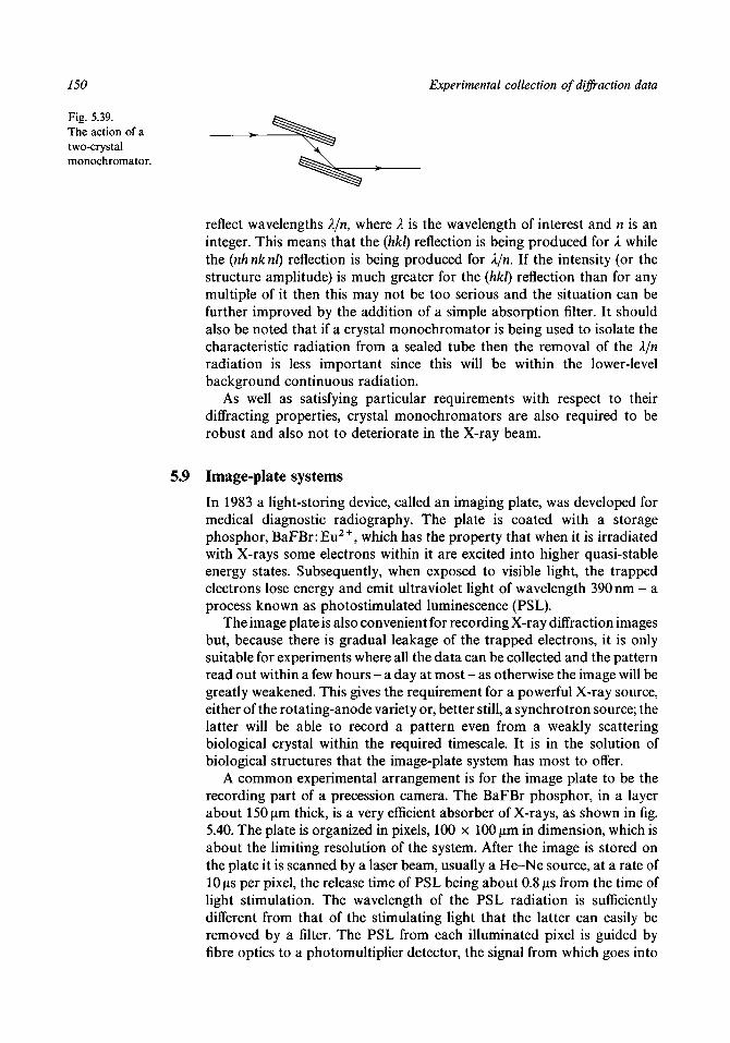
150
Fig. 5.39.The action of atwo-crystalmonochromator.
Experimental collection of diffraction data
reflect wavelengths X/n, where X is the wavelength of interest and n is aninteger. This means that the (hkl) reflection is being produced for X whilethe (nh nk nl) reflection is being produced for X/n. If the intensity (or thestructure amplitude) is much greater for the (hkl) reflection than for anymultiple of it then this may not be too serious and the situation can befurther improved by the addition of a simple absorption filter. It shouldalso be noted that if a crystal monochromator is being used to isolate thecharacteristic radiation from a sealed tube then the removal of the X/nradiation is less important since this will be within the lower-levelbackground continuous radiation.
As well as satisfying particular requirements with respect to theirdiffracting properties, crystal monochromators are also required to berobust and also not to deteriorate in the X-ray beam.
5.9 Image-plate systems
In 1983 a light-storing device, called an imaging plate, was developed formedical diagnostic radiography. The plate is coated with a storagephosphor, BaFBr: Eu2 + , which has the property that when it is irradiatedwith X-rays some electrons within it are excited into higher quasi-stableenergy states. Subsequently, when exposed to visible light, the trappedelectrons lose energy and emit ultraviolet light of wavelength 390 nm - aprocess known as photostimulated luminescence (PSL).
The image plate is also convenient for recording X-ray diffraction imagesbut, because there is gradual leakage of the trapped electrons, it is onlysuitable for experiments where all the data can be collected and the patternread out within a few hours - a day at most - as otherwise the image will begreatly weakened. This gives the requirement for a powerful X-ray source,either of the rotating-anode variety or, better still, a synchrotron source; thelatter will be able to record a pattern even from a weakly scatteringbiological crystal within the required timescale. It is in the solution ofbiological structures that the image-plate system has most to offer.
A common experimental arrangement is for the image plate to be therecording part of a precession camera. The BaFBr phosphor, in a layerabout 150 \im thick, is a very efficient absorber of X-rays, as shown in fig.5.40. The plate is organized in pixels, 100 x 100 jum in dimension, which isabout the limiting resolution of the system. After the image is stored onthe plate it is scanned by a laser beam, usually a He-Ne source, at a rate of10 is per pixel, the release time of PSL being about 0.8 s from the time oflight stimulation. The wavelength of the PSL radiation is sufficientlydifferent from that of the stimulating light that the latter can easily beremoved by a filter. The PSL from each illuminated pixel is guided byfibre optics to a photomultiplier detector, the signal from which goes into

5.10 The modern Laue method 151
Fig. 5.40.The absorption of theimaging phosphorBaFBr:Eu2+ as afunction of wavelength.The absorption edge at0.330 A is due tobarium.
100
•2 50
i i i i
0.2 0.4 0.6 0.8 1.0
Wavelength (A)
1.2
a digital storage and image-processing system. A representation of such asystem is shown in fig. 5.41. The intensity of the PSL is linearly related tothe X-ray intensity over a wide range of about l:105. There is a littlebackground noise in the system, due to the photomultiplier tube forexample, but it is no worse than for film. Again, there are usually somevariations of sensitivity in different parts of the image plate but these arenormally less than 1.6%.
The sensitivity, dynamic range and precision of image-plate systemsgive them a growing role in X-ray crystallography, particularly in theanalysis of biological crystals.
5.10 The modern Laue method
The very first X-ray photograph, produced by Friedrich and Knipping in1912, was taken with a stationary crystal and, effectively, a continuoussource of X-rays. The picture was crude but was good enough to verify vonLaue's idea that crystals could diffract X-rays. From the Bragg point of viewin the Laue experimental arrangement the reflecting planes correspondingto the (hkl) reflection are fixed in direction, as is the normal to those planes.The angle between the direction of the incident radiation and the normal isalso fixed but if that angle is ^n — 6 for some wavelength present in theincident beam then radiation of that wavelength will form a reflected(diffracted) beam.
In general, Laue photographs are very difficult to decipher and the onlysimple information they give is when the incident beam is aimed along asymmetry axis, when the diffraction pattern will clearly show a correspondingsymmetry (see §7.3). A characteristic of the Laue method is that all thediffracted beams are produced at the same time and this can have importantadvantages, particularly for protein crystallography. One of the greatproblems with biological crystals is that they are degraded by X-rays so thatif the same crystal is used for a long time the quality of the data steadily getsworse. The degradation of the crystal is not just due to the total X-ray dosebut also involves a time element. The X-rays produce free radicals withinthe crystal by breaking off extremities of the protein molecules and it is thediffusion of these through the crystal that seems to do the damage.Traditionally this problem of crystal decay has been met by using

152 Experimental collection of diffraction data
Fig. 5.41.The scanningmechanism for animage-plate system. Atthe end of eachlaser-beam scan theplate is moved in thedirection shown, by thedimension of one pixel.
Scanning
Limits of scan
Motionof plate
Laser beamTo photomultiplier,data storage andimage processing
Opticalfibres
-200 mm
individual crystals for only a limited time so that a whole batch of crystalswould be required to collect a single set of data. The Laue method offers analternative approach since, in conjunction with a synchrotron source, it cangive a data set in a fraction of a second. Another possible application is if anexperiment is carried out on the crystal, say exposing it to a laser beam,causing it to undergo some short-lived structural change. This change maythen be investigated by recording its Laue diffraction pattern while it is inthe transient state.
A Laue diffraction photograph taken with synchrotron radiation for acrystal of the protein concanavalin A is shown in fig. 5.42. While it is quite acomplicated pattern it can be seen that the reflections all lie on families ofcurves. Knowing the orientation of the crystal it is possible to calculate theposition of each diffraction spot and hence to index every spot on the film.There are, nevertheless, some problems to be solved. The first, and thesimplest, is that since each spot corresponds to a different wavelength ofX-radiation then it is necessary to interpret the intensity of a spot relative tothe power spectrum of the source, which is well known for synchrotronradiation and possibly also the quantum efficiency of the film for differentX-ray wavelengths.
The second problem is a little more difficult and can be understood interms of Bragg's law, equation (3.37). This can be written as
(5.25)
where dhkl is the spacing of the reflecting planes for the Miller indices (hkl). Ifwe now consider the reflection with Miller indices (nh nk nl) then
dnh,nk,nl = dhkl/n
and we may write
(5.26)
A/n(5.27)

5.10 The modern Laue method 153
Fig. 5.42.Laue photograph of theprotein concanavalin Ataken with DaresburySRS wiggler radiationwith exposure time of19 ms. Under theconditions of theexperiment Amin = 0.5 Aand Amax = 2.0 A.(Courtesy of J. R.Helliwell.)
This means that in the Laue photograph all the spots for reflections(nh nk nl) will overlap for all n.
The problem is not quite as bad as it might seem at first sight. The X-raysfalling on the crystal have an upper and lower wavelength limit - 2.0 A and0.5 A, respectively, for conconavalin A so that n cannot be greater than 4 forany reflection. Again if a reflection such as the (17 38 2) is recorded then noreflection with smaller indices can be coincident with it, because 17 is aprime number, and no reflection with higher indices will be present if themaximum possible k index is less than 76. In general, it has been shown byCruickshank and Helliwell that for most realistic experimental arrangementsmore than 85% of reflections on Laue pictures should be single spotswithout overlap and 95% should be either without overlap or singlyoverlapped. Even when there is overlap the problem of separating theintensities due to the components is possible in principle. This is achievedby having a multiple film pack separated by layers of absorbing material.The absorption of X-rays in materials is wavelength dependent (§6.2). Letus assume that two diffraction spots overlap corresponding to reflection(hkl) with wavelength X and reflection (2h 2k 21) with wavelength A/2 and thecombined intensity on the top film is
IT = / i + I2 (5.28)
where lx is the intensity due to reflection (hkl) and I2 is that due to reflection

154 Experimental collection of diffraction data
(2h2k2l). If the absorber reduces the intensity of radiation of wavelength Xby a known factor ax and that of wavelength X/2 by a known factor a2 thenthe intensity on the bottom film is given by
JB = aj, + a2l2. (5.29)
From equations (5.28) and (5.29) the separate components in the top filmmay be found as
and
I2 = (aJT - JB)/(a x - a2). (5.30)
With three films separated by two layers of absorbing material it should bepossible similarly to unravel the intensities of three overlapped spots on thetop film.
The problems of the Laue method are such that crystallographers willusually prefer to use methods involving moving crystals and monochromaticradiation but for special applications the Laue approach is a usefuladditional technique.
Problems to Chapter 5
5.1 A crystal has an orthorhombic unit cell with a = 11.4 and c = 8.9 Aand can be rotated about the b axis. An incident beam of Cu Karadiation (X = 1.54 A) falls on the crystal normal to the rotation axis.The crystal is in the reflecting position for the (907) reflection. By whatangle must it be rotated for the (702) reflection to be produced?
5.2 (a) An oscillation photograph is taken with Cu Ka radiation therotation being about an axis of length 7.2 A. If the camera diameteris 57.3 mm find the distances of the layer lines h = 1, 2, 3 from thezero-layer line.
(b) An oscillation photograph is taken with Cu Ka radiation and giveslayer lines whose distances from the zero-layer line are as follows:
h = 1 4.5 mm,h = 2 9.3 mm,h = 3 14.9 mm.
The camera diameter is 57.3 mm. What is the length of the a axis?5.3 For a certain crystal a* = 0.15, b* = 0.20 A " 1 and y* = 80°. When a
15° oscillation photograph is taken with Cu Ka radiation about the caxis, reflections are produced in the zero-layer line making thefollowing angles with the incident beam. To right looking in directionof beam - 13°, 41°, 61°, 75°, 85°, 102°, 125°, 152°. To left looking indirection of beam - 13°, 48°, 62°, 78°, 90°, 114°, 116°, 130°, 152°.
What are the indices of these reflections? Which reflections in theobservable range are too weak to be observed?
5.4 A normal-beam zero-layer Weissenberg photograph is taken with CuKa radiation giving the (hkO) reflections for an orthorhombic crystal for

Problems to Chapter 5 155
which a = 8.0 and b = 6.0 A. When the crystal is at the end of itstraverse the X-ray beam points straight down the a axis. Find thecoordinates on the film of all possible reflections of the type 1/cO andT/cO. Plot these on a replica of fig. 5.19(fo) and confirm that they followthe form of the curves shown in that figure.
Assume that the oscillation is through 180°, the diameter of thecamera is 57.3 mm and the translation constant of the film is 0.5 mm perdegree of rotation.
5.5 The energy of the electrons in a synchroton is 3.0 GeV and the bendingmagnet fields are LIT. What is the critical wavelength and the verticaldivergence of the emitted radiation?
It is required to reduce the critical wavelength to 0.5 A with awiggler. What field must be produced by the wiggler magnets?
5.6 A Laue photograph, which is known to have overlapping (231) and(462) reflections is recorded on two films separated by an absorbinglayer. On the top film the sum of the intensities of the overlapped spotsis 262 and on the lower film 106. The absorber allows through 30% ofthe shorter-wavelength radiation and 60% of the longer-wavelengthradiation. What are the individual intensities of the two spots on thetop film?

6 The factors affecting X-ray intensities
6.1 Diffraction from a rotating crystal
It has been seen that methods of recording X-ray intensities usually involvea crystal rotating in the incident X-ray beam. We shall now look at theproblem of determining the total energy in a particular diffracted beamproduced during one pass of the crystal through a diffracting position. Inorder to do this we must make some assumptions about the geometry of thediffraction process; the configuration we shall take is that the crystal isrotating about some axis with a constant angular velocity co and that theincident and diffracted beams are both perpendicular to the axis of rotation.
Let us first look at the situation when we have a stationary crystal in adiffracting position. Associated with the crystal, and fixed relative to it,there is a reciprocal space within which is defined the Fourier transform,Fx(s), of the electron density of the crystal. For a theoretically perfect crystalof infinite extent the value of Fx(s) would be zero everywhere except at thenodes of a (5-function reciprocal lattice, the weight associated with the point(hkl) being (l/V)Fhkl. However, if the crystal is imperfect in some way theremay be non-zero Fx(s) well away from the reciprocal-lattice points and for afinite crystal there will be a small region of appreciable Fx(s) around each ofthe reciprocal-lattice points. The imperfect-crystal case we shall notconsider here but we shall be concerned with the size of the crystal, for this isa factor which must be present in every diffraction experiment.
Consider a crystal completely bathed in an incident beam of intensity /0.The crystal will reflect over a small range of angles around the 'ideal'position for a reflection (hkl); in a particular position corresponding to anangle 6 let the power of the reflected beam be (dE/dt)e. This power is clearlyproportional to / 0 and one can define the reflecting power by
where P(0) is a quantity with the dimensions of area.In fig. 6.1 there is shown a typical curve relating P(0) to 6. Because of
various factors such as divergence of the incident beam and crystalimperfection the detailed shape of this curve is less important than the totalarea under the curve. This area phkl is called the integrated reflection.
Thus when the crystal is rotated with an angular velocity co ( = dO/dt)
156

6.1 Diffraction from a rotating crystal 157
Fig. 6.1.A typical curve forreflecting power as afunction of 6.
P(0)
dd
coE,hkl (6.2)
where Ehkl is the total energy in the diffracted beam when the crystal sweepsthrough the diffracting position. We shall now examine the problem offinding Ehkl.
We saw in §3.1 that a finite one-dimensional array of scatterers givessome scattering away from the directions of the main peaks and the same istrue for a finite three-dimensional lattice. Let us assume that we have, say,aniVfl x Nb x iVc three-dimensional array of point electrons with the arraydefined by the vectors a, b and c. In a direction corresponding to a scatteringvector s the intensity of scattering can be found by a simple extension of theresults in §3.1 and by applying equation (2.22) as
L^S-« electrons ^0 sin2(7ta's) sin2(ixb#s)
sin2(7iiVcC's)
sin2(7ic*s)
The component of equation (6.3)
sin2(7iiVfla*s) sin2(iiiVbb#s) sin2(7iNcc*s)
(6.3)
( f l ) ( b ) ( c
sin2(7ia*s) sin2(7tb*s) sin2(7ies)
is a 'shape factor' associated with the distribution of intensity around eachreciprocal-lattice point. As in the one-dimensional case, illustrated by fig.3.2, this factor will give the same shape of distribution about eachreciprocal-lattice point.
Clearly as 5 -• 0 so the height associated with this peak tends to N^NlN*while the width in each of the primary directions, i.e. the distance at whichthe factors first fall off to zero, is of order (Naa)~l, (N^)'1 and (JVcc)-1,respectively. Hence the total weight associated with the 'shape factor' is oforder (NaNbNc)/(abc) = N/V where N is the total number of unit cells in thecrystal and V the volume of the unit cell. This rough assessment will beconfirmed later.

158 The factors affecting X-ray intensities
Fig. 6.2.The intersection of asmall region of thecrystal Fourier transformas a shaded area roundthe point P, with thesphere of reflection.
Let us now examine this question in more detail. In fig. 6.2 the crystalmay be considered at C, the centre of the sphere of reflection, while theorigin of Fx(s) is situated at O. In general the value of Fx(s) over the surface ofthe sphere will be small unless a reciprocal-lattice point lies on or very nearthe surface which is the condition we have previously noted for a diffractedbeam to occur. We may consider that the incident X-ray beam is scatteredin all directions; if at the point P in fig. 6.2 the value of the transform is Fx(s)then this means that in the direction CP the intensity of scattering, «/s, is| Fx(s)|2 times that which would result from a point electron at C. Hencefrom equation (2.22) we may write
21 + cos2 20,F,(s)|2 (6.4)
and in a small solid angle dQ in the direction CP the total scattered energyper unit time is Js dQ.
The situation for the particular diffraction geometry we are consideringwhen the crystal is passing through a diffracting position is shown in fig.6.3(a). The reciprocal-lattice point P, with indices (hid), has associated withit a small volume, represented by the ellipsoidal surface, within whichresides all the intensity associated with this particular reflection. Of courseno such sharp boundary really exists; surfaces of constant intensity need notbe ellipsoidal and what is shown is purely illustrative. The volume is shownjust entering the sphere of reflection and its surface of intersection with thesphere is that shown shaded which has total area a. Within this surface isshown a very small area da; this subtends an angle X2da at C and the totalenergy scattered through it in time dr is
dEhkl = (6.5)
and hence the total energy scattered during the total time T of the passage of

6.1 Diffraction from a rotating crystal 159
Fig. 6.3.(a) A schematic view ofthe passage of theregion round areciprocal-lattice pointthrough the sphere ofreflection as the crystalrotates.(b) The small shadedvolume between Q andQ passes through thearea a on the sphere ofreflection as the crystalrotates through anangle codt.
it)the small volume through the sphere of reflection is
JT Ja(6.6)
It should be noted that as time changes so different cross-sections of thevolume pass through the sphere. In fig. 6.3(b) the plane COP is shown andthe area da at Q on the surface of the sphere. The crystal, and its associatedreciprocal space, rotates by an angle codt in a time dt and the transformsurface da moves to Q while P moves to F. It can be seen that a volumedadz of the transform moves through the small element of surface of thesphere. From the diagram it is easily seen that if

160 The factors affecting X-ray intensities
OQ = s( = ——^ ) then dz = scos0 x codt. (6.7)\ * /
The integration (6.6) can now be rewritten as
z Jascocos</>(6.8)
which, since dadz is an element of volume in reciprocal space, can also beexpressed as
Ehkl=
Jsdv (6.9)
since (j) =^= 9 for the whole region of interest around the reciprocal-latticepoint. The effect of replacing point electrons by the electron distribution ina unit cell is to give the complete distribution of electron density in thecrystal and the intensity of scattering from this is
$ _ r <f I v I F 12 (fi 1 CY\^ S ~~ L^sJ electrons * I r hkl I ^O.IU/
where we now assume that we are only interested in s at, or very close to, thereciprocal-lattice point (hkl). Substituting from equations (6.3) and (6.10)into equation (6.9)
_ P / e2 yi+cos220*" " ^ ° \4Ti80c
2m) 2 sin 29 ' hkl'
f sin2(7iiVfla-s) sin2(?i Nbb-s) sin2(nNcc-s)
JVhki sin2(7ia*s) sin2(7cb's) sin2(7ic*s)
The integral in equation (6.11) should be taken in a region around thereciprocal-lattice point (hkl) but, as we have already noted, the shape factoris the same for all reciprocal-lattice points and so we can carry out theintegration around the origin.
It is convenient to consider a set of coordinate axes with a*, b* and c* asthe units of measurement along the three appropriate axial directions.
Then a point s in reciprocal space will have coordinates (rj, £, Q so that
s = rja* 4- £b* + Cc*. (6.12a)
This leads to
a#s = rj, b#s = <!;, c#s = C (6.12b)
and a volume element is given by
dv = F*df/d^dC (6.12c)
where F* is the volume of the reciprocal unit cell.We may now rewrite equation (6.11) as
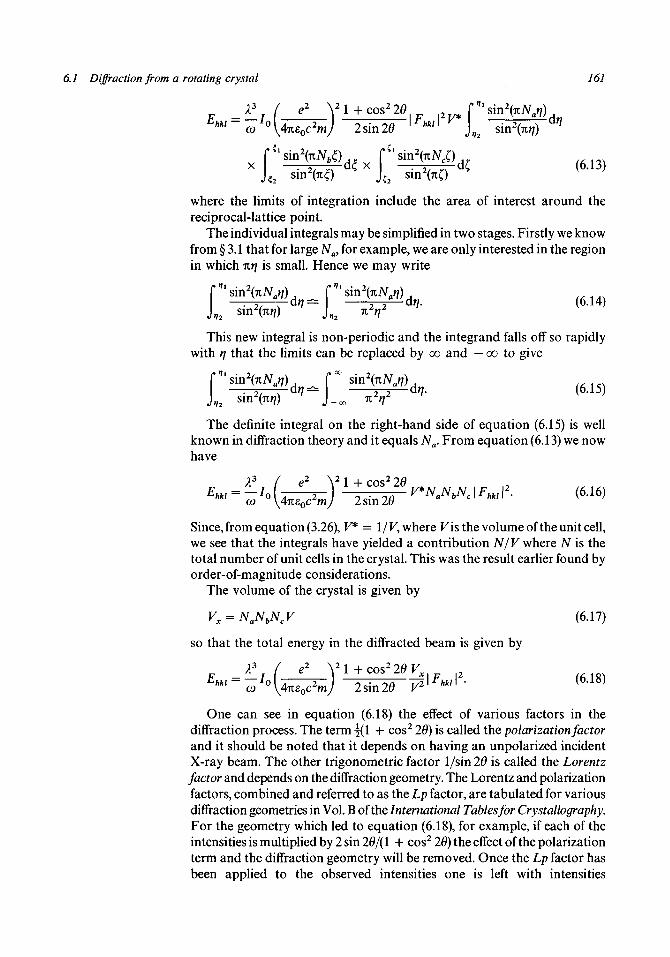
6.1 Diffraction from a rotating crystal 161
EhkI~ coIo{4ns0c2m) 2sin20 | F M I | 2 K * J , 2 s i r 2 ' - - ^
1 sin2
where the limits of integration include the area of interest around thereciprocal-lattice point.
The individual integrals may be simplified in two stages. Firstly we knowfrom § 3.1 that for large Na, for example, we are only interested in the regionin which nrj is small. Hence we may write
This new integral is non-periodic and the integrand falls off so rapidlywith rj that the limits can be replaced by oo and — oo to give
rj) J n2rj2,2 sm2(nrj) J . ^ n2rj
The definite integral on the right-hand side of equation (6.15) is wellknown in diffraction theory and it equals Na. From equation (6.13) we nowhave
Since, from equation (3.26), K* = 1/V, where Kis the volume of the unit cell,we see that the integrals have yielded a contribution N/V where N is thetotal number of unit cells in the crystal. This was the result earlier found byorder-of-magnitude considerations.
The volume of the crystal is given by
Vx = NaNbNcV (6.17)
so that the total energy in the diffracted beam is given by
X3 ( e2 \ 2 l + c o s 2 2 0 F , „ IO
One can see in equation (6.18) the effect of various factors in thediffraction process. The term ^(1 + cos2 29) is called the polarization factorand it should be noted that it depends on having an unpolarized incidentX-ray beam. The other trigonometric factor 1/sin 26 is called the Lorentzfactor and depends on the diffraction geometry. The Lorentz and polarizationfactors, combined and referred to as the Lp factor, are tabulated for variousdiffraction geometries in Vol. B of the International Tables for Crystallography.For the geometry which led to equation (6.18), for example, if each of theintensities is multiplied by 2 sin 26/(1 + cos2 26) the effect of the polarizationterm and the diffraction geometry will be removed. Once the Lp factor hasbeen applied to the observed intensities one is left with intensities

162 The factors affecting X-ray intensities
proportional to | Fhkl\2 (ignoring other corrections) and, as we shall see in
chapter 8, these intensities are required if one is to solve the crystal structure.It is instructive to look at the effect of the crystal size on the energy in the
diffracted beam. This is seen in equation (6.18) to be proportional to thevolume of the crystal; it must be pointed out that although equation (6.18)was derived for a regular parallelepiped-shaped crystal it is applicable toany shaped crystal. If the volume of the crystal is doubled then, from theresults in § 3.1, it appears that the intensity in the direction of the diffractedbeam will be increased fourfold. However, with the larger crystal thedistribution of intensity around the reciprocal-lattice point is more condensedand effectively occupies one-half the previous volume. This means that theoverall increase in total energy is just doubled, i.e. is proportional to thevolume of the crystal used.
Let us find the order of magnitude of the total energy in a diffracted beamfor a typical situation. A typical copper X-ray tube of 1 kW rating probablydelivers about 1 watt of characteristic Kot X-rays which is emitted over asolid angle of 2n steradians (a hemisphere). The crystal will be about100 mm from the target and if we assume that the radiation is emitteduniformly and that the collimator allows the crystal to be completelyexposed to X-rays, then the intensity of the incident X-ray beam is
We now take
20 = TI/2
A=1.54AK x =10- 1 2 m- 3
F=500A3
co = 0.05 radians s
and we find
This is equivalent to a number of X-ray photons
n = he
From the values of h, Planck's constant, =6.63 x 10 3 4Js and c, thevelocity of light, =3 x 10⁸ms"1 we find for this example n= = 104.
6.2 Absorption of X-rays
When X-rays pass through a material their intensity is attenuated byabsorption, that is the conversion of the energy of the electromagneticradiation to thermal energy, and also by scattering. In fig. 6.4 there isdepicted an X-ray beam of intensity / having its intensity changed to / + d/

6.2 Absorption of X-rays 163
Fig. 6.4.The attenuation of anX-ray beam afterpassing through a smalldistance in a material.
by passage through a thickness dx of material. The law which will always befound to hold is
Fig. 6.5.The variation of the pathlengths of the incidentand diffracted beams fordiffraction from differentregions of the crystal.
d /_
/ ~ "
or, integrating and putting I = Io when x = 0,
i = 1 r>e
(6.19)
(6.20)
The quantity n is known as the linear absorption coefficient of the materialand it has the dimension of inverse distance. The quantity exp( — fix) isknown as the attenuation factor.
If we examine fig. 6.5 the effect of absorption on the intensity of the X-rayreflection can be seen. An incident beam entering a crystal would, but forthe effect of absorption, have the same intensity at all points of the crystal -for example at the points P and Q. In addition, without absorption, smallequal volumes in the vicinity of P and Q would give equivalent contributionsto the emergent diffracted beam. When absorption is taken into account itcan be seen that the incident beam at P will have a lesser intensity than at Qbecause of the longer path to P in the crystal and in fact the intensity at Pwill be IOQ~^XP while that at Q is IOC~^XQ. Similarly the diffracted beam fromP will be more attenuated in going from P to P' than does that going from Qto Q\ the attenuation factors being e " ^ and e~"*Q, respectively. Thediffracted beam from F is reduced in intensity by absorption by a factorQ-n(xp+X£) an (j tke pOSition is similar for all other points in the crystal.
If the crystal was an ideal, perfect crystal we should have to take accountof the coherence of the radiation scattered from different parts of the lattice.

164 The factors affecting X-ray intensities
Fig. 6.6.A schematic diagram ofa mosaic crystal.
This would mean a modification of the theory from which equation (6.18)was derived since, in this theory, absorption was ignored. However, as willbe seen later, for such a perfect crystal the simple theory is, in any case,inadequate in a more fundamental way. In practice perfect crystals are rareand usually we have what approximate to ideal imperfect crystals of the typeillustrated schematically in fig. 6.6. The crystal consists of a mosaic of smallblocks, each block being perfect but separated by faults and cracks in thecrystal from other blocks. The small blocks are usually of the order of a fewmicrons in dimensions, the gaps between them are non-parallel and ofrandom thickness so clearly there can be no systematic relationshipbetween the phases of radiation scattered from different parts of the crystalwhich are in different blocks. Thus to get the total intensity of scatteringfrom the complete crystal we add the intensities of the radiation scatteredfrom different regions of the crystal. For the crystal shown in fig. 6.7,assumed ideally imperfect, the small volume dv will contribute to thediffracted beam an intensity proportional to Q~tl(x+X)dv. The fraction bywhich the total intensity is reduced by absorption is given by
.= fJV
(6.21)
Fig. 6.7.The contribution to thediffracted beam of smallvolume dv is reduced byabsorption by a factorexp{ - fi(x + *')}•
When fi is large the absorption factor A can have a large effect and mustbe corrected for if accurate results are required from the eventual structuredetermination. If, for example, we have a platy crystal similar to that shownin fig. 6.8(a) then for one reflection most rays have a path like ABC while foranother reflection the rays might be similar to DEF. If the incident anddiffracted rays are all in the plane of the plate then one can determine theapproximate value of A by a graphical method. The crystal cross-section isdivided into a number of equal areas, for example the ten shown in fig.6.8(b), and the centres of these areas are found - Ox to O1O in the figure. We

6.2 Absorption of X-rays 165
Fig. 6.8.(a) For a crystal of veryunequal dimensionsabsorption correctionscan vary greatly fromreflection to reflection.(b) Approximategraphical method ofcalculating absorptionfactors by dividingcrystal into smallregions.
HIM
(a)
now approximate the integral (6.21) by the summation
(6.22).?where the total area is divided into M smaller areas. For the example shownin fig. 6.8(2?) the details of the calculation, assuming ju = 5 x 10³m"1,follow in table 6.1. From equation (6.22) this gives A = 0.044. The accuracyof this method of calculating absorption factors is increased if a greaternumber M of points is taken but, of course, the labour involved in thecalculation also increases. Computer programs have been written tocalculate absorption factors; some of these are very sophisticated and willcompute values of A for crystals of somewhat irregular shape. However if itis possible to shape the crystal by grinding it into a sphere or a cylinder thenabsorption factors can be expressed in the form of tables and these are givenin Vol. B of the International Tables for Crystallography. For a sphere ofradius R, for example, the absorption factor is a function of fiR and sin 6only and can be very concisely tabulated.
We shall now take a look at some general aspects of absorption with aview to discovering the general rules which govern it and also to findinghow to determine \i for materials of known composition.
The simplest materials to consider are those which consist of a singleelement. For the attenuation of a beam going through such material onemay write
— (6.23)
where dn is the number of atoms in the path of the beam per unit area and/ia, which depends on the element, is known as the atomic absorption

166 The factors affecting X-ray intensities
Table 6.
Point (0
123456789
10
1.
X-
All linear
0.140.430.140.430.140.430.140.430.140.38
x;dimensions
0.140.140.420.420.690.470.970.471.270.47
Xi + Xiare in mm
0.280.570.560.850.830.901.110.901.410.85
M*, + x;
1.402.852.804.254.154.505.554.507.054.25
;.) exp{ - n{xt + x;.)}
0.24710.05780.06080.01440.01590.01120.00390.01120.00090.0144
coefficient. If experiments are done to measure /ia as a function of thewavelength of the X-radiation the results appear as in fig. 6.9. Starting witha long wavelength, say at the point P, the value of /ia steadily reduces as Xdecreases. The X-ray photons, with energies he/A, will have more energy forsmaller X and hence one should expect them to be more penetrating.However if the wavelength is reduced to the value of Q the value of /ia
sharply increases and then, with a further reduction of X, /ia decreases again.These sudden discontinuities in atomic absorption coefficient - and thereare several of them - are known as absorption edges. They can beunderstood in terms of the electronic structure of the atom. Within theatom, electrons exist in definite energy states and the absorption edgescorrespond to energies hc/X which are just sufficient to eject an atomicelectron from the atom. At the point P the photon energy is insufficient toeject any of the electrons of an unexcited atom and the photons eitherinteract with the whole atom increasing its energy of motion, which isequivalent to increasing its temperature, or lose energy through theCompton effect. However at Q the photons have just enough energy to ejectan Lm shell electron; a new mechanism for interaction of the photon and theatom becomes available and results in a sharp increase in absorption.Similar effects occur corresponding to the other atomic electrons and givesa whole series of absorption edges. Between the absorption edges thegeneral fall-off of the absorption curves follows a form close to
fia = CZ*X5/2 (6.24)
where Z is the atomic number of the material and C is a constant whichdepends on the nature of the two flanking absorption edges.
Equation (6.23) can be transformed to be in terms of the distancetraversed by the beam. In fig. 6.10 the slab of material has unit cross-sectionalarea, and thickness dx. If it contains dn atoms then the total mass ofmaterial is Mdn/NA where M is the atomic weight and NA is Avogadro's
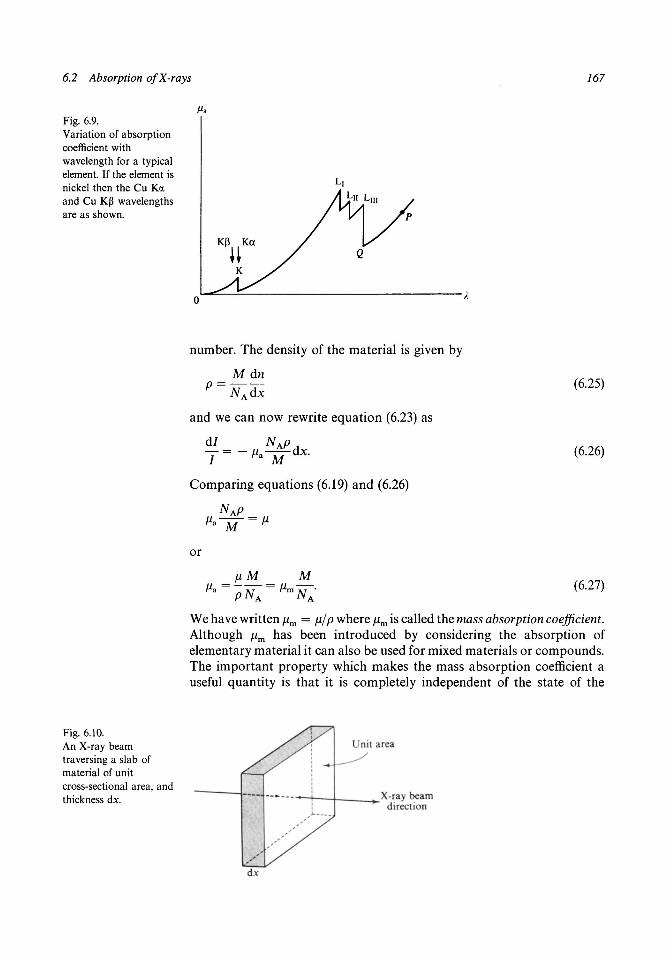
6.2 Absorption of X-rays 167
Fig. 6.9.Variation of absorptioncoefficient withwavelength for a typicalelement. If the element isnickel then the Cu Kaand Cu Kp wavelengthsare as shown.
K|3 Ka
number. The density of the material is given by
_ M d n
and we can now rewrite equation (6.23) as
(6.25)
(6.26)
Comparing equations (6.19) and (6.26)
M
or
M(6.27)
We have written fim = \ijp where jum is called the mass absorption coefficient.Although }im has been introduced by considering the absorption ofelementary material it can also be used for mixed materials or compounds.The important property which makes the mass absorption coefficient auseful quantity is that it is completely independent of the state of the
Fig. 6.10.An X-ray beamtraversing a slab ofmaterial of unitcross-sectional area, andthickness dx.
Unit area
X-ray beamdirection

168 The factors affecting X-ray intensities
material. This means that jnm = JJL/P is the same for
ice, water and steam;graphite and diamond;solid and liquid sulphur;solid CO2 and CO2 gas.
Thus if one tabulates for elements their mass absorption coefficients forvarious wavelengths then linear absorption coefficients for elements can bededuced no matter in which state they exist. Thus the value of jxm for theelement carbon for X = 1.54 A is 0.460m2 kg" x and from this we can findthe linear absorption coefficient for the three forms of carbon - diamond,graphite and amorphous carbon black. Thus
/'diamond = (/Oc + diamond = 0.460 X 3.52 X 103 m " * = 1.62 X 10³ Hi" */White = fan)c + Pgraphite = 0.460 X 2.25 X 103 Hi" ' = 1.03 X 10³ m~ X
Amorphous = (/Oc + Pamorphous = 0.460 X 1.88 X l O ^ " 1 = 0.86 X lO 3 !*" 1
This same principle can be extended to determine the linear absorptioncoefficients of mixtures of elements or compounds by using the relationship
/'compound = Z /'element = Z ftnPp (6.28)
where the summations are taken over all the elements in the compound andpp represents the partial density of the element within the compound. Anexample will illustrate more clearly how one uses this equation. We shalldetermine the attenuation of a beam of Cu Ka radiation (X = 1.54 A) inpassing through a slab of NaCl of thickness 0.1mm.
The following information can be found in tables:
Density of NaCl = 2.2 x 10³kgm" 3
Na atomic weight 23 fim(X = 1.54 A) = 3.0m2 kg"1
Cl atomic weight 35 [im(A = 1.54A) = 10.6m2kg"1.
The proportion of the two elements by mass is Na: Cl = 23:35 so thatthe partial densities are
and
(pp)cl = 2 . 2 x 10³ x f f k g m " 3 .
Thus
\i = (2.2 x ff x 3.0 + 2.2 x H x 10.6) x 103m"1
= 1.67 x 10⁴m"1.
The attenuation factor for the beam is then given by equation (6.20) and isexp(-1.67 x 104 x 10"4) or 0.188.
By such means one can determine linear absorption coefficients for anymaterial when the individual elemental mass absorption coefficients andthe density and composition of the material are known. Mass absorptioncoefficients for the elements are listed in Vol. C of the International Tablesfor Crystallography.

6.3 Primary extinction 169
In § 5.8 the use of absorption filters to remove unwanted radiation froman X-ray source was mentioned. For example, a sealed copper tube will giveas its main characteristic output Cu Ka and Cu K(3 radiation of wavelengths1.542 and 1.389 A, respectively, and it is usually required to remove theshorter-wavelength component. The K absorption edge for copper, whichis the energy required to eject an electron from the K shell, must be at awavelength shorter than either the Ka or K0 radiations. However, theelement one less in atomic number than copper is nickel (atomic number 28)and its K absorption edge falls between the CuKa and CuKfS wavelengths.If fig. 6.9 represents the atomic absorption coefficient of nickel then the CuKa and Cu K|3 wavelengths are shown as Ka and K|3. It is clear that theabsorption is far less for the Ka radiation. For example, the massabsorption coefficients of Ni for Cu Ka and Cu K(3 radiations are 4.57 and27.5 m2 kg"1, respectively. The density ofNi is 8.9 x 10³kgm~3 and hencethe linear absorption coefficients are 4.1 x 10⁴m~1 and 24.5 x 10⁴m~1.Afoil of thickness 20 fim ( = 2 x 10~5m) transmits a fraction 0.44 of the Karadiation but only 0.0075 of the K(3 and thus constitutes a very efficient filter.
6.3 Primary extinction
So far in our consideration of diffraction from a crystal we have assumedthat the atoms are under the influence of an incident beam whose intensityhas been modified only by absorption in the crystal. However if we look atfig. 6.11, in which is represented the passage of the incident X-ray beamthrough the material and the formation of the diffracted beam, it is clearthat this simple picture is not really true. Every point in the crystal is underthe influence of the incident beam and also some part of the diffracted beamwhich is moving in a different direction. If the crystal is in a stronglyreflecting position the extra effect of the diffracted beam component will notbe negligible.
We shall first investigate the propagation of a plane wave through acrystal in the direction of the incident radiation. We imagine that theX-radiation is 'established' in the crystal which is therefore occupied by acontinuum of radiation. In fig. 6.12 there is represented a section in which
Fig. 6.11.A schematicrepresentation of theformation of a diffractedbeam originating frompoints distributedthroughout the crystal.
Incident, beam
Diffractedbeam

170 The factors affecting X-ray intensities
Fig. 6.12.(a) The formation of aplane wave front fromwavelets originatingfrom a plane ofscatterers.(b) All radiationoriginating in theannular region arrive atP with the same phaserelationship.
New w a v e front
O l d w a v e front
there are scatterers through a plane labelled Q1 to Q5. Most of the radiationpassing through the plane <2i2s will n o t t>e scattered and will eventuallypass through the plane containing the point P in a time which depends onthe distance Q3P. However some small part of the X-radiation will bescattered by the scatterers Q so that the point P, for example, is at any timealso receiving some radiation coherently scattered by each of the points Q.We imagine that the points Q are sufficiently densely packed so that theplane containing them may be considered as a uniform partially scatteringplane.
It is clear from fig. 6.12(6) that radiation from all the points on the ring ofradius r will arrive at P with the same phase relationship. The phase lagbehind the radiation coming from Q will be
* < 4 >
or
The phase lag ar with respect to the unscattered radiation coming from Qis given by
(6.29a)
where the % is the Thomson scattering phase shift.For r = 0, ar = % and the first part of our phase-vector diagram,
illustrated in fig. 6.13(a), starts from O and is directed in the direction AO -that is along the negative real axis.

6.3 Primary extinction 171
Fig. 6.13.{a) Phase-vectordiagram for radiationoriginating from aplane of scatterers andarriving at a plane wavefront. The resultant,OC, is 7t/2 ahead inphase of the radiationarriving from thenearest scatterer.{b) Radiation goingalong OA without beingscattered is reduced inintensity due todestructive interferencewith radiation doublyscattered at C and O.
(a)
By differentiating equation (6.29a) we find
Inrdrr X(r2 + d2)r (6.29b)
On the phase-vector diagram the contribution of a small annular regionof radius r and thickness dr will be a line segment, dqr, whose length will beproportional to the area of the annulus and inversely proportional to thedistance s. This latter factor is equivalent to an inverse-square-law fall-offfor intensity.
Thus we have
dqr = r 2nrdr
\r2+d2f(630)
where K is some constant. Taken together, equations (6.29b) and (6.30) give,dropping the subscript r,
(6.31)
The geometrical shape corresponding to equation (6.31), where thechange of angle is proportional to arc length, is a circle. With only the
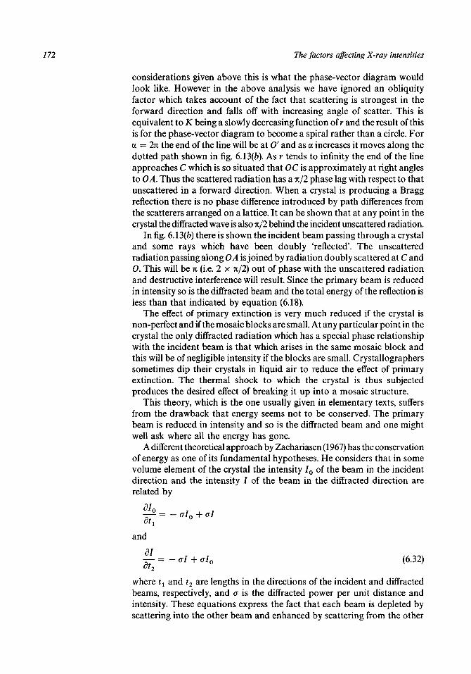
172 The factors affecting X-ray intensities
considerations given above this is what the phase-vector diagram wouldlook like. However in the above analysis we have ignored an obliquityfactor which takes account of the fact that scattering is strongest in theforward direction and falls off with increasing angle of scatter. This isequivalent to K being a slowly decreasing function of r and the result of thisis for the phase-vector diagram to become a spiral rather than a circle. Fora = 2it the end of the line will be at 0' and as a increases it moves along thedotted path shown in fig. 6.13(6). As r tends to infinity the end of the lineapproaches C which is so situated that OC is approximately at right anglesto OA. Thus the scattered radiation has a n/2 phase lag with respect to thatunscattered in a forward direction. When a crystal is producing a Braggreflection there is no phase difference introduced by path differences fromthe scatterers arranged on a lattice. It can be shown that at any point in thecrystal the diffracted wave is also n/2 behind the incident unscattered radiation.
In fig. 6.13(5) there is shown the incident beam passing through a crystaland some rays which have been doubly 'reflected'. The unscatteredradiation passing along OA is joined by radiation doubly scattered at C andO. This will be n (i.e. 2 x n/2) out of phase with the unscattered radiationand destructive interference will result. Since the primary beam is reducedin intensity so is the diffracted beam and the total energy of the reflection isless than that indicated by equation (6.18).
The effect of primary extinction is very much reduced if the crystal isnon-perfect and if the mosaic blocks are small. At any particular point in thecrystal the only diffracted radiation which has a special phase relationshipwith the incident beam is that which arises in the same mosaic block andthis will be of negligible intensity if the blocks are small. Crystallographerssometimes dip their crystals in liquid air to reduce the effect of primaryextinction. The thermal shock to which the crystal is thus subjectedproduces the desired effect of breaking it up into a mosaic structure.
This theory, which is the one usually given in elementary texts, suffersfrom the drawback that energy seems not to be conserved. The primarybeam is reduced in intensity and so is the diffracted beam and one mightwell ask where all the energy has gone.
A different theoretical approach by Zachariasen (1967) has the conservationof energy as one of its fundamental hypotheses. He considers that in somevolume element of the crystal the intensity / 0 of the beam in the incidentdirection and the intensity / of the beam in the diffracted direction arerelated by
and
^L = - cl + alo (6.32)
where tx and t2 are lengths in the directions of the incident and diffractedbeams, respectively, and a is the diffracted power per unit distance andintensity. These equations express the fact that each beam is depleted byscattering into the other beam and enhanced by scattering from the other

6.4 Secondary extinction 173
beam into itself. The sum of the two equations gives
which is the condition for the conservation of energy. These equations areaugmented by the boundary conditions that, where the incident beamenters the crystal, /0 equals the intensity of the incident X-ray beam and / = 0.
The coupling constant a is clearly a function of £, the angle the beammakes with the 'ideal' direction as given by Bragg's equation and clearly afalls off very rapidly with s and is significantly only for small s.
We cannot explore here the full depth of Zachariasen's treatment of theseequations but a selection of the solutions he obtains will give the generalpattern of his results.
The factor by which the diffracted intensity is reduced for a sphericalspecimen and for low scattering angles is given by
(6.34)
where Ms the mean path length in the crystal and equals \r for radiationpassing straight through a sphere.
For small aT this is approximately
0() Lot
(6.35a)
which is an exact solution for an infinite plane parallel plate when theincident and reflected beams make the same angle to the normal to the plate.
When the crystal has a mosaic structure, with domain size smallcompared to that of the whole crystal, the result corresponding to equation(6.35a) is
(6.35b)
where Tis the mean path through the whole crystal and 6 a mean o for thedistribution of orientations of the domains. Since d is less than the value of ofor a perfect crystal a reduction in primary extinction results from mosaicstructure.
6.4 Secondary extinction
It is found that even when a crystal is ideally imperfect, consisting of verysmall mosaic blocks, there is another type of extinction process which mayoccur. We have already found that the intensity of an X-ray beam isattenuated by its passage through a material by the absorption of some ofthe X-ray energy and its conversion to thermal energy. This process is quiteindependent of the phenomenon of diffraction and could be recorded bymeasuring the attenuation of a beam of X-rays passing through slabs ofmaterial. However when the crystal is in a diffracting position there isavailable another mechanism for removing energy from the incident beam -that is to say, that some of the energy goes into the diffracted beam. In fig.6.14 the passage of the incident beam, of initial power 70a, through a small

174 The factors affecting X-ray intensities
Fig. 6.14.Effective increase inabsorption coefficientdue to diffraction.
Cross-sectionalarea i
P(0)Io
mosaic element of a crystal is illustrated. The emergent beam power isdepleted firstly by an amount filoat due to ordinary absorption andsecondly by an amount equal to P(0)/o (equation (6.1)) which is a measureof the power of the diffracted beam from this small element of the crystal.The overall result of this additional depletion is effectively to raise the linearabsorption coefficient from // to //(0) where
(6.36a)
where Q(0) is the reflecting power per unit volume of the mosaic element.For a complete sweep of the crystal through a reflecting position there willbe some average // given by
Q(0). (6.36b)
The magnitude of \i — \i can be very considerable; for example someexperiments by Bragg, James and Bosanquet (1921) with rock salt crystalsshowed that, for the (200) reflection with Rh Ka radiation {X = 0.613 A), thevalue of // = 1.630 x 10 3 m" 1 whereas the normal linear absorption co-efficient is only 1.070 x H^m" 1 .
This phenomenon is known as secondary extinction and it is difficult toeliminate by any treatment of the crystal. It certainly can be reduced tosome extent by increasing the imperfection of the crystal. Secondaryextinction can be thought of as a shielding effect which exists at a point in acrystal due to diffraction by the layers of crystal above it - that is, closer tothe incident X-ray beam. If the mosaic blocks were all precisely parallel thenall of them would diffract simultaneously and the secondary extinctioneffect would be the same as that for a perfect crystal. However if the mosaicblocks have a range of orientations then they do not all diffract together asthe crystal is rotated and the shielding effect is consequently reduced. Onewould not expect to find secondary extinction with a powder sample whereonly a tiny fraction of the crystallites are diffracting at any one time.
Since secondary extinction is equivalent to a change in the linearabsorption coefficient of the material of the crystal its proportional effect onintensities is reduced if very small crystals are employed. This can beillustrated by the example shown in fig. 6.8(fc) and table 6.1. If the value of//is 5.5 x 10³m"1 (// = 5.0 x 10³m~1) then the numbers in the columnn(xt + x[) are all increased by 10% and the value of A changes from 0.044 to0.035 or by about 19%. If we now consider a crystal similar in shape but

6.5 The temperature factor 175
with its dimensions reduced by a factor of two we find A^ = 0.165 andA p. = 0.145, a change of 12%. A further reduction by a factor of two in thedimensions gives A^ = 0.381 and A^. = 0.349 and secondary extinctionnow gives a 6% reduction of intensity. However this reduction of crystalsize and reduction of secondary extinction is bought at the expense oflowering the diffraction intensities, so in practice there is a limit to thesmallness of the crystal which can be used. For the most part crystallographersaccept that only a few very strong reflections will be affected by secondaryextinction and these do not usually interfere with the processes ofdetermining or refining crystal structures.
6.5 The temperature factor
The picture we have created of a crystal is that of a rigid stationaryassemblage of atoms bound together in a periodic pattern. We must nowconsider how the picture is modified by the presence of thermal energybecause thermal energy on the atomic scale is energy of motion.
Every atom in a crystal structure is bound to numbers of other atoms bybonding forces of various types and the position of the atom is thatcorresponding to the minimum potential energy. It is probably rather moreaccurate to say that the complete crystal structure corresponds to anarrangement of minimum potential energy and where, for example, asubstance crystallizes in two different forms it means that two arrangementsexist with potential energies virtually equal to each other and lower thanthat of any other arrangement. If an atom is disturbed from its equilibriumposition it experiences a restoring force tending to move it back again andwe can see that the atom can acquire thermal energy by oscillating about itsequilibrium position. Thus we get a modified view of a crystalline solid inwhich all the atoms are vibrating about their mean positions withamplitudes which increase as does the temperature of the solid. Thesevibrations will affect the relative coordinates of the atoms and hence thediffraction pattern and we shall now investigate this phenomenon.
The first thing to note is that the frequencies of vibration of atoms arevery low in relation to the sort of times in which we are interested - forexample the time of transmission of X-rays through the crystal. For thisreason we may imagine that, at any instant of time, the diffraction patternbeing produced is that of a 'frozen' crystal in which all the atoms arestationary and displaced by some distance from their mean positions. Thetotal intensity pattern that we get over any long period of time is atime-average of the patterns which are obtained at successive instants. Weare going to assume that all the atomic vibrations are completely uncorrelatedso that averaging processes can be carried out for individual atoms.
To begin with let us take one unit cell of a one-dimensional structurecontaining N atoms per unit cell where thejth atom has mean fractionalcoordinate xj and, at some instant of time, an absolute displacement fromthat position uy If all the other unit cells were in a precisely similar state thestructure factor of index h would be given by

176 The factors affecting X-ray intensities
" ( U \= £ ffxp 2nih -^ exp(27ii/zx), (6.37)
7=1 \ a /
The actual structure amplitude in a direction corresponding to h will be atime and space average of equation (6.37) since Uj varies from one unit cell tothe next and, within one unit cell, varies with time.
We write for the structure factor at some temperature T
[7/Jr = £ ffi*P (2nih^)exp(2iufac,) (6.38)
where exp{2nih(Uj/a)} is the average value of the diplacement term. In allpractical cases Uj is small enough to be able to write approximately
expf Inih^- ) = 1 + Inih^- - 2n2h2% (6.39)\ aJ a a
For simple harmonic or other symmetrical vibrations u} = 0, so we have
\" 2
2iii/z— j = 1 — 2n2h2 -^ (6.40a)
or, in a more convenient form,
exp ( 2icifc^ ) ^ exp f - 2n2h2 %\ (6.40b)
\ fl/ V a )The result (6.40b) substituted in equation (6.38) together with h/a = 2 sin 6/Agives
JV
l 7 J r = E/;exp(-87i2w?sin20/i2)exp(27ii^). (6.41)7 = 1
It can be seen that the overall result of the thermal motion of the atoms iseffectively to modify their scattering factors to
UJ]T =ffxp(-Sn2u2sm2e/A2). (6.42)
If the three-dimensional case is now considered it will be found that theequation corresponding to (6.42), without the introduction of 6, appears inthe form
/ 2 7 i 2 ( s - u / } . (6.43)
Now
(s*Uj)2 = 52w2 cos2 (j) (6.44)
where 0 is the angle between the vectors s and u,- and since we areconsidering a particular s and since Uj and (/> are independent of each otherwe may write
(s'U •) = s Uj cos (j). (6.45)
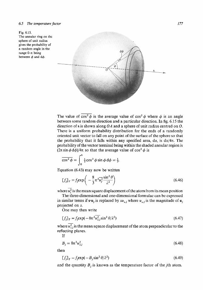
6.5 The temperature factor 177
Fig. 6.15.The annular ring on thesphere of unit radiusgives the probability ofa random angle in therange O-it beingbetween <p and d<£.
The value of cos2 (j) is the average value of cos2 4> where <f> is an anglebetween some random direction and a particular direction. In fig. 6.15 thedirection of s is shown along OA and a sphere of unit radius centred on 0.There is a uniform probability distribution for the ends of a randomlyoriented unit vector to fall on any point of the surface of the sphere so thatthe probability that it falls within any specified area, da, is da/47i. Theprobability of the vector terminal being within the shaded annular region is(27i sin (j) d(j))/4n so that the average value of cos2 <j) is
cos2(/>=
Equation (6.43) may now be written
(6.46)
where u] is the mean square displacement of the atom from its mean positionThe three-dimensional and one-dimensional formulae can be expressed
in similar terms if S'u, is replaced by su±j where u±j is the magnitude of u7-projected on s.
One may then write
T = fjQxp( - j sin2 9/X2) (6.47)
where u2Lj is the mean square displacement of the atom perpendicular to the
reflecting planes.If
= 8TL2W2;= 8TL2W
then
UJ]T =ffxp(- 9/A2)
(6.48)
(6.49)
and the quantity Bj is known as the temperature factor of the jth atom.

178 The factors affecting X-ray intensities
Fig. 6.16.(a) Atom B vibratesmost strongly in theplane perpendicular toAB.(b) Atoms Q and Rshould have a largeramplitude of vibrationthan does atom P.
We have tacitly assumed above that the vectors u, have an equalprobability distribution in space - an assumption of vibrational isotropy.In fact this is rarely so and the magnitude and mode of vibration of an atomwill depend very much on its environment. By and large, less energy isinvolved in changing bond angles than in changing bond lengths, so that anatom out on a limb, so to speak, as illustrated in fig. 6.16(a), will tend tooscillate mainly in the directions perpendicular to the bond. The quantity[/}]T, the scattering factor of the vibrating atom, is the Fourier transform ofthe time-average of the electron density for the range of positions taken upby the vibrating atom. If an electron-density map is computed with thestructure factors [Fhk J T for all h, k and / then for thejth atom one will see thetime-averaged electron density. Similarly if one had a group of atoms of thetype shown in fig. 6.16(b) the atom P will move mainly at right angles to thebond NP. Vibration of the bond NP will also affect the atoms Q and Rwhose motion is augmented even more by vibrations of the bonds PQ and PR.
In general, the surfaces of constant time-averaged electron densityapproximate to ellipsoids and in the most precise crystal-structure analysesthe parameters which describe these ellipsoids are determined (see §9.3).However for all but the most accurate work it is usually sufficient to assumethat the thermal vibrations are isotropic and that the values of B are thesame for all atoms. In that case we have
or for intensities
(6.50)
(6.51)
The factor by which the observed intensities are reduced by thermalvibrations, exp( — 2Bsin2 6/A2), is known as the Debye-Waller factor.
Directions ofoscillation inplane perpendicularto AB
(a)
(b)

6.6 Anomalous scattering 179
Table 6.2.
Debye-Waller factor, exp( - IB sin2 0/k\ for three values of B (in A2)
sin 0/A
0.20.40.60.81.0
2.0
0.85210.52730.23690.07730.0183
2.5
0.81870.44930.16530.04080.0067
3.0
0.78660.38290.11530.02150.0025
Typical values of temperature factors fall in the range 2-3 A2 and, toillustrate their order or magnitude, Debye-Waller factors are given in table6.2 for various values of B and sin 6/L
For B = 3 A2, for example, and for the limit of Cu Ka radiation(sin 6/A = 0.65), it will be seen that the intensity is reduced to about 10% ofits unmodified value.
The dependence of B on the absolute temperature Thas been theoreticallyinvestigated by Debye who produced a formula whose application islimited to materials which are elements. If© is the characteristic temperatureof the material and x = &/T then the formula is
, ,52,
where
m is the atomic mass,h is Planck's constant,kB is Boltzmann's constant
and
f ^ r d £ .xjo e x p ^ - 1
In practice the value of B can be found from the experimentallydetermined values of ^hkl; the method of doing this is described in §7.5.
6.6 Anomalous scattering
In determining scattering factor equations as in § 2.6 it has been assumedthat all the atomic electrons are unrestrained and undamped so that thescattering phase shift is % for each of them. If we consider one atomicelectron, moving independently of all the others, then its vibrational motionin the alternating electric field of an incident electromagnetic wave might begoverned by an equation of the form
mx + gx + kx = Eoe exp(iatf). (6.53)
180 The factors affecting X-ray intensities
In equation (6.53) m is the electron mass, k the restoring force per unitdisplacement, Eo and co/2it are the amplitude and frequency of the incidentwave and it is assumed that there is a damping force gx proportional to thevelocity.
The steady-state solution of this equation is
x = ^exp(icor) (6.54a)
where
Eoe Eoe[(k - co2m) - i
(k — co2m) + igco (k — co2m)2 + g2co2
Another form of solution, without recourse to complex notation, is
x = R cos(cot + s) (6.55a)
where
Eo*
and
t a n s = - , gC°2 . (6.55c)k — arm
For an unrestrained and undamped electron one would have k = 0 and= 0 giving
x= -^eXp(icot). (6.56)CD YYl
This represents an oscillation of the electron with the same frequency as theoncoming wave but 71 out of phase with it - as is shown by the negativeamplitude. By writing equation (6.56) as
x = J ^ i exp{i(cor + 7i)} (6.57)
the phase shift of n with respect to the oncoming wave E = E0Qxp(icot) ismade more evident.
When/c # 0 there is a resonance frequency corresponding toco = co0 where
k — a>lm = 0
so that we may write
k = colm. (6.58)
Substituting this in equation (6.54b) we obtain
(col — co2)2m2 + g2co2 (col ~~ a)2)2m2 + g2co2
When co = co0 and the damping constant g is small it can be seen that theamplitude of oscillation of the electron would be very large. In our presentclassical model the amplitudes of vibration of atomic electrons are

6.6 Anomalous scattering 181
continuously and infinitely variable. However, from a quantum-theorypoint of view, the angular frequency co0 is that for an X-ray photon with justenough energy to eject the electron from the atom, i.e. that which has awavelength corresponding to the absorption edge.
The critical wavelength Xo is given by
Xo = — (6.60)
and Xo would correspond to one of the absorption-edge wavelengths shownin fig. 6.9.
The electrons which are most tightly bound to the nucleus and thereforehave the highest value of k are the K electrons but, even for these, we can seefrom equation (6.59) that when co » co0 their behaviour is not very differentfrom that of a free electron. Thomson-scattering theory is only trulyapplicable for co -> oo and in the vicinity of an absorption edge the vibrationof the electron, and hence its scattering, will be very different from thatpredicted by the Thomson formula. The amplitude of the scattered wavewill be proportional to the amplitude of the electron vibration; we canexpress the real and imaginary components of the amplitude of thescattered wave as fractions of that from a free electron by dividing thecomponents in equation (6.59) by the amplitude given in equation (6.56).These fractions are, for the real part,
— (O2)m2
^ = (co20 - co2)2m2 + g2ao2
and, for the imaginary part,
(6.61a)
gco3m<t>B = j—2 2X2~2 2~^- (6.61b)
{col - co2)2m2 + g2co2
For a Thomson-scattering electron one would have <\>A = 1 and cj)B = 0so that, if the absolute Thomson contribution to the scattering factor of thiselectron is p0, then the actual contribution is
Po = Poi^A= Po + Pi + P2I (6-62)
where
= nJrh . — W = ^OQ — co ) m + g2co
-q2co2
Pi = POWA - 1) = ,°.2 J'2 ^ „" , Po (6.63a)
and
Let us consider a diffraction situation where we have an iron atom in thecrystal and Cu Ka radiation {X = 1.54 A) is being used. The K absorptionedge for iron is at 1.74 A and is at a greater wavelength for all the otherabsorption edges so that we might expect the two K electrons to scatteranomalously (i.e. other than as free electrons) while the others would be

182 The factors affecting X-ray intensities
closer in behaviour to free electrons. For the two wavelengths concerned
co = 1.224 x lO^s" 1 and co0 = 1.083 x 10 1 9s~\
If we write
— = ij/— (6.64)m co
then we find
<t>A = ^ (6.65a)
and
. 4 .61^cpB = 2- (6.65b)
The actual behaviour of the electrons will depend very much on the valueof \j/ or, what amounts to the same thing, on the value of g.
One possible mechanism which would give us an estimate of the value ofg is the radiation of energy by the electron - that is to say, that g is aradiation-damping constant. In fact this does not tie in with our picture of aharmonically vibrating electron because the greatest radiation of energy,and therefore the greatest damping resistance, occurs when the accelerationis greatest which, for a simple-harmonic motion, is when the velocity isleast. By writing the damping term as gx in equation (6.53) we have implied,on the contrary, that the damping force is proportional to the velocity.However we can calculate an order-of-magnitude value for a meandamping constant g. It can be shown by a simple extension of equation(2.18) that an electron vibrating with an amplitude R emits energy at anaverage rate
(6.66)6 = 1 2 ^
The total distance it travels in unit time is
D = 4R x frequency = (6.67)71
and therefore the mean force it experiences due to the radiation of energywould be
F Q e2Ra}3
The mean velocity of the electron also equals D so that the average force perunit velocity becomes
_ F ne2co2
We can test this mean value of damping constant to see whether or not it

6.6 Anomalous scattering 183
gives sensible values for the scattering fractions cf)A and cj)B when theincident radiation has the wavelength of the absorption edge, or is veryclose to that wavelength. For co = co0 we have
cj)A = 0
and
co0m 48goc3m<PB = — = 2— (6-70)
or, when numerical values are substituted, cf)B = 1.2 x 10⁴. This very largevalue, which implies that the electron is vibrating with 1.2 x 10⁴ times theamplitude of a Thomson electron, shows that radiation damping is far toofeeble to offer an explanation of the anomalous scattering effects which areactually observed.
Another approach which can give us a rough estimate of g is byconsideration of the mass absorption coefficient of the element in question.If the K absorption-edge wavelength is being scattered then the two Kelectrons should be oscillating more strongly than any others. Let usassume that the damping force, whatever its origin, is the mechanism bywhich X-radiation is absorbed by the atom and transformed into heat. Thedamping force acting on the electron is gx and when it moves through adistance dx does work
d W = gxdx = gx2dt
or, from equation (6.55a),
d W = gR2co2 sin2(cot + e)dt. (6.71)
Since the average value of sin2(cot + e) is \ we have as the rate of loss ofenergy through damping forces for each K electron
o2. (6.72)
When co = co0, R = E0e/gco0 so that
A us F2p2
^ r = 2 • (6-73)
Now let us consider the situation when the radiation passes through athin slab of material of thickness dx and of unit cross-sectional area. If thereare N absorbing electrons per unit volume then the total energy absorbedper unit time by passing of the beam is
° dx. (6.74)
If the intensity of the incident beam is / then this is also the energy passinginto the block per unit time and equation (6.74) represents the change of thisintensity, say d/. For an electromagnetic wave the electric-field strength andintensity are related by

184 The factors affecting X-ray intensities
I = E2cs0 (6.75)
so that
Ne2
d / = - - Idx. (6.76)2gcs0
The negative sign is put into equation (6.76) to indicate a reduction of theintensity of the beam; we can now compare equations (6.76) and (6.19) to obtain
Ne2
= u2gcs0
or
Ne2
^ (6.77)
where \i is the linear absorption coefficient of the material.If the density of the material is p and the atomic weight M then the
number of atoms per unit volume is
n = ^ N A (6.78)
where NA is Avogadro's number and if we assume two fully effective Kelectrons for each atom then N — 2n and
9 =
For an iron atom at its K absorption edge fim = 46 m2 kg "* and M = 56 sothat
If this value of g is used for all frequencies then <\>A and cj>B can becomputed as a function of frequency or wavelength. The results of thiscalculation are shown in table 6.3.
Now the K electrons are the ones most tightly bound to the nucleus ofthe atom and the ones which most closely resemble point electrons. It willbe noticed in fig. 2.12(fo) that the scattering contribution of the K electronsof carbon do not fall off very rapidly with sin 0/L For an iron atom wherethe K electrons are even more tightly bound the fall-off will be even less and,for a reasonable range of sin 0/A, may be neglected altogether.
From equation (2.38), if we refer to the normal atomic scattering factor as/0, then we have
/o = i iPshJ = I
If the non-anomalous contribution of the two K electrons is taken to beunity for each then we can write the actual scattering factor as

6.6 Anomalous scattering 185
Table 6.3.
Afl.
0.000.250.500.751.001.251.501.752.00
1.001.061.311.990.00
-1.42-0.75-0.47-0.33
<t>B
0.000.060.200.774.420.710.200.090.08
/ i = 2{(j>A - 1)
0.000.120.621.98
-2.00-4.84-3.50-2.94-2.66
0.000.120.401.548.841.420.400.180.16
i/2 (6-80)
where
/ i = 2{(t>A - 1) (6.81a)
a n d
f2 = 2<\>B. (6.81b)
The terms/i and/2 are, respectively, the real and imaginary changes inthe scattering factor due to anomalous scattering and these are shown intable 6.3 and in fig. 6.17.
It should not be expected that this rather crude theory based on classicalideas should give good agreement with experiment but it does give areasonable qualitative picture. A quantum-mechanical treatment ofanomalous scattering has been given by Honl (1933) and the resultsobtained for iron from this theory are shown in fig. 6.18. The general form ofthe classical solution is quite good except that it predicts a finite f2 forX > /lK whereas the quantum-mechanical theory gives / 2 = 0 under thiscondition.
An important consequence of anomalous scattering is that it causes abreakdown of Friedel's law. Let us consider a non-centrosymmetricalstructure containing five atoms in the unit cell. The separate contributionsof the five atoms to the (hkl) and (Ek 7) structure factors can be shown on aphase-vector diagram as in fig. 6.19(a) and the equality of | Fhkl \ and | FMT\can be seen. However if the scattering factor of the fifth atom has anomalouscomponents then | Fhkl | is no longer equal to | F^T\. Let the contribution toFhkl of the other four atoms be R exp(/0) and the scattering factor of the fifthatom b e / + if. Then
Fhkl = #exp(i(/>) + (/ + i//)exp(27iir5-s)= [Kcos(/> +/cos(27iiys) — /'sin(27iiys)]
+ i[R sin 0 + / ' cos(27ir5-s) +/sin(27ir5-s)] (6.82)
and similarly
FMT= [Rcoscj) +/cos(27tiys) +/'sin(27ir5's)]+ i[R sin 4>+f cos(27tiys) -/sin(27ir5-s)]. (6.83)

186 The factors affecting X-ray intensities
Fig. 6.17.The anomalousscattering components/ i and f2 for iron fromthe classical theory.
1.0
From equations (6.82) and (6.83) it will be seen that | Fhkl | ^ | F^j\. Thisbreakdown of Friedel's law is also shown in fig. 6A9(b) where it will be seenthat the effect of the anomalous-scattering component, apart from a smallchange in the magnitude of t h e / is to rotate the contributions to FhM andFMJboth in the same sense. The reader may readily confirm by drawingsimilar diagrams that, for centrosymmetric structures, Friedel's law is retained.
Anomalous scattering can be an important aid to structure determinationand the method by which this is done is described in §8.5.

6.6 Anomalous scattering
Fig. 6.18.The anomalousscattering components/i and f2 for iron fromthe quantum-mechanical theory.
187
Si
10-
1.0 2.0

188 The factors affecting X-ray intensities
Fig. 6.19.(a) Friedel's law for anon-cent rosymmetricstructure withoutanomalous scattering.(b) The breakdown ofFriedel's law with oneanomalous scatterer.
(b)
Problems to Chapter 6
6.1 A crystal of volume 10~ 9m" 3 is rotated about its c axis at an angularvelocity of 0.02 radians sec ~*. A beam of Cu Ka radiation (X = 1.54 A)of intensity lOWm" 2 is incident on the crystal at right angles to theaxis of rotation. The structure is orthorhombic with a = 6.0, b = 12.0and c = 10.0 A. How many photons will there be in the (240) diffractedbeam for a single passage through the reflecting position if | F2401 = 120?
6.2 A material of density 1.28 x 10³ kgm" 3 has the chemical compositionC1 4H2 2S2P2. What is the linear absorption coefficient of the materialfor Cu Koc radiation?

0.04 m2 kg" 1
0.467.419.81
1123132
Problems to Chapter 6 189
Element nm{k = 1.54 A) Atomic weight
HCPS
6.3 The crystal in Problem 6.1 is a block with sides parallel to a, b, c oflengths 2.00, 1.00 and 0.50mm, respectively. If the linear absorptioncoefficient of the material is 5.0 x 10³m"1 what is the absorptionfactor for the (240) reflection? Use the graphical method described in § 6.2.
6.4 Recalculate the structure factors in Problem 3.4 if the overall temperaturefactor for the structure is 3.0 A2. The program STRUCFAC (appendixI) can be used for this calculation.
6.5 A crystal of space group PI with a = 10.00, b = 7.00 and y = 110° has aprojection with the following structure:
Atom
BrNCCccc
Calculate the structure factors of type (hkO) with STRUCFAC for CuKot radiation (X = 1.542 A), given that the overall temperature factor is3.0 A2 and that bromine has anomalous scattering components/i = — 0.96 and/2 = 1.46. Note the breakdown of Friedel's law.
0.6250.3000.4000.3000.4250.5250.525
0.2500.6430.2860.4290.7140.5710.393

7 The determination of space groups
7.1 Tests for the lack of a centre of symmetry
As we have seen in § 1.4 measurements of crystals with an opticalgoniometer can, in favourable circumstances, reveal the crystal class. Suchmeasurements should be carried out on many crystals for there is atendency for crystals to exist in a number of slightly different forms in eachof which some facets may not be present. By-and-large, when incorrectconclusions are drawn from optical goniometry it is in the direction ofassigning too high a symmetry to the crystal. However it is sometimespossible to be reasonably sure by means of such measurements that acrystal structure either has or does not have a centre of symmetry.
There are a number of physical properties of crystals, the measurementsof which can be used unequivocally to detect the lack of a centre ofsymmetry in a crystal structure. We shall briefly consider these, the physicalprinciples involved and the apparatus which may be used for the tests.
Piezoelectric effect
The first physical phenomenon we shall consider is that of piezoelectricity.This is the process whereby when a material is placed in an electric field itundergoes a mechanical strain and, conversely, when the material ismechanically strained it becomes electrically polarized and produces a fieldin its environment. Let us see what mechanism can produce this effect. Infig. l.\(a) there is a schematic representation of a pair of atoms with theirsurrounding electron density. The two atoms are bonded together and theelectron density is distorted from the configuration it would have for thesuperposition of that from two isolated atoms. The distortion is in the senseof building up extra electron density in the bond between the atoms whichtends to attract the nuclei inwards and hence keep them together. If the pairof atoms is placed in an electric field this will lead to a displacement of thenegatively charged electron cloud with respect to the positively chargednucleus. It may happen that the outer electrons of atom B are more shieldedfrom the nucleus than are those of atom A and hence they may more easilybe displaced. Consequently the net migration of electrons, as shown in fig.7.1(6), may be such as to enhance the build-up of electron density in thebond. This will have the effect of attracting the two nuclei inwards and so ofshortening the bond. This diminution in bond length would be small anddependent on the first power of the field; if the direction of the field wasreversed then some electron density would move out from between thenuclei and the bond length would increase.
For a crystalline material the field will produce an induced polarizationand all the bonds would be affected in one or other of the two possible ways,and in varying degrees, so that the aggregate effect would be to change thephysical dimensions of the crystal. The sign of the change of dimensions
190

7.1 Tests for the lack of a centre of symmetry 191
Fig. 7.1.(a) Representation ofelectron densityassociated with a pairof bonded atoms.(b) Change of electrondensity in an electricfield.
(b)
would depend on whether the shortening or lengthening of bondspredominates. However it should be noted that an overall effect can onlyoccur for a non-centrosymmetric crystal. In fig. 1.2(a) a one-dimensionalcrystal structure is illustrated and it will be seen that there are four differenttypes of bond which, depending on their nature, can give an overall increaseor decrease in the dimension of the crystal. On the other hand, for thecentrosymmetric structure shown in fig. 7.2(2?) there will always be pairs ofbonds, such as AB and A'B\ whose contributions to the change ofdimensions are equal and opposite so that there is no externally observableeffect.
The piezoelectric effect is reversible so that, if the material is physicallystrained, the electronic charge will flow in and out of the regions betweennuclei. The net flow of charge will lead to a polarization of the material andhence a field will be produced around it. This effect is used in the quartz-controlled oscillator, the natural frequency of one of the modes ofmechanical vibration of the crystal controlling the electrical oscillation of acircuit coupled to it.
A very simple type of piezoelectric-effect tester is shown in fig. 7.3. The

192 The determination of space groups
Fig. 7.2.(a) A one-dimensionalnon-centrosymmetricstructure; no bonds inone unit cell are related.(b) A one-dimensionalcentrosymmetricstructure; bonds exist inpairs in oppositedirections.
(a)
A
OB B'• o o •
A'O o o • O o o
(b)
sample, in the form of a large number of crystals, is placed between theplates of a condenser which is in series with a variable-frequency oscillatorand a loudspeaker. At any particular frequency the current in the circuit willdepend on how many of the crystals have a mode of vibration at, or close to,that frequency. The frequency of the oscillator is well above the audio rangeand so nothing is heard from the loudspeaker. When the frequency is slowlychanged however, the vibrations of the various crystals go in and out ofresonance and a series of clicks is heard from the loudspeaker.
Fig. 7.3.A piezoelectric-effectdetector.
Variable-frequency oscillator
Crystals
Loudspeaker
It must be emphasized that while the detection of the piezoelectric effectcertainly denotes the lack of a centre of symmetry no conclusion is possiblefrom a negative result as the piezoelectric effect may be present but just betoo feeble to be detected. In addition Wooster (1938) showed that thesymmetry of one point group, 43 2, does not permit a piezoelectric effect.
Pyroelectric effect
Another physical property which can be detected in non-centrosymmetriccrystals is that of pyroelectricity. This is the electrical polarization of acrystal shown by the development of opposite charges on two oppositefaces of a crystal when it is heated. In fact since a crystal must always be atsome temperature it suggests that pyroelectric crystals should be polarizedeven at room temperature and, if this is not observed, it is because thecharges on the surface are usually neutralized by stray charges on particlesof dust, etc. Thus it is inferred that in a pyroelectric crystal there existspermanent polarization which suggests the presence of electric dipoles

7.1 Tests for the lack of a centre of symmetry 193
within the crystal. If this is so then the additional polarization due toheating can be ascribed to asymmetric oscillation of the dipoles. In fig. 7.4the situation is depicted where on heating the crystal the mean distanceapart of the charged atomic groups, and therefore the mean dipole momentis increased by raising the temperature.
A very simple form of pyroelectric test is to insert into a specimenconsisting of small crystals a heated glass rod. If the crystals are pyroelectricthey will develop charges on their surfaces, induce opposite charges on therod, and so adhere to it. The precaution should be taken of repeating theexperiment with a cold rod to ensure that some other effect is not causingthe adhesion.
The above test is not a very sensitive one and other types of test arepossible. However tests for pyroelectricity are rarely performed bycrystallographers so we shall pursue this topic no further.
Fig. 7.4.Asymmetric oscillationsof charged groups giverise to increased meandipole moment astemperature increases.
Mean positions of chargedgroups at room temperature
Oscillationsinduced by heating
Optical activity
A material is said to be optically active if, when plane-polarized light passesthrough it the plane of polarization is rotated. Some materials, such asquartz and certain inorganic salts, are optically active in the crystalline statebut not when fused or dissolved in solution. This means that it is the specificarrangement of atoms in the crystal that determines the optical activity.There are other substances, notably organic molecular substances, whichare optically active when crystalline, molten, vaporized or in solution, andfor these the optical activity is clearly a property of the molecular structure.
When materials are optically active they often exist in two forms whichrotate the plane of polarization in opposite senses. If looking towards thesource of light gives a clockwise rotation the crystal is said to bedextro-rotatory; otherwise it is laevo-rotatory. The two contrary-rotatingforms of the material are enantiomorphs, that is to say that structurally theyare mirror images of each other. Sometimes this shows itself in the crystalsthemselves, the sets of normals to the faces being mirror related in the twotypes of crystal. Clearly centrosymmetrical structures cannot be opticallyactive since centrosymmetrically related objects are also enantiomorphicallyrelated and a centrosymmetric structure is its own enantiomorph. The sameis true of structures with planes of symmetry or inversion axes.
For organic materials the optical activity is associated with the tetrahedral

194 The determination of space groups
Fig. 7.5.(a) Enantiomorphicallyrelated four-bondedcarbon atoms.(b) Enantiomorphicforms of tartaric acid.
arrangement of bonds around a carbon atom bonded to four other atoms.This is illustrated in fig. 7.5(a) for two carbon atoms with four differentatoms attached to each; the two arrangements are enantiomorphicallyrelated. In fig. 1.5(b) two enantiomorphically related molecules of tartaricacid are shown.
It is not too simple to observe optical rotation from crystals because, aswe shall see in the following section, light passing through any other than acubic crystal is usually split into two components polarized at right angles.If the crystals are soluble then the solution can be tested by means of theapparatus shown in fig. 7.6. The light is plane-polarized by a polarizer P (aNicol prism or polaroid sheet for example) and after passing through thetube of solution traverses the analyser A. The polarizer and analyser areinitially adjusted so as to give no passage of light when the tube is full ofsolvent. If light passes through when the solvent is replaced by solution thenthe dissolved crystals must consist of molecules of one enantiomorph andso the space group cannot be centrosymmetric. However no conclusion canbe drawn if optical activity is not detected. The effect might be too small tobe detected or the crystals may be a mixture of the two enantiomorphic
w w
(a)
HO OH
OH HO
OH HO
(b)

7.1 Tests for the lack of a centre of symmetry 195
Fig. 7.6. P A
A simple polarimeter.
Solution
forms (racemic mixture) and hence neutralize the effect of each other insolution.
Frequency doubling
Light is propagated in materials by inducing vibrations of the chargedcomponents, mainly electrons, within it. If for a region round a smallelement of charge there is a lack of symmetry then the vibration of thecharge element in an electric field due to a light wave can be anharmonic.This is only likely to occur appreciably at high fields (high intensity of light)and the general form of the vibration is shown in fig. 7J(a). It is due to thefact that the restoring force per unit displacement of charge is a variable andis less for displacements in one direction than for the other. Let us assumethat the vibration has the form
x = A cos cot(l + a cos cot) (7.1)
which is that shown in fig. U(a) with a = 0.2. Then
x = \Ai 4- A cos cot + \Au. cos 2cot (7.2)
and it can be seen that the displacement has a constant component which isequivalent to a polarization of the material and also one of twice theincident frequency.
The effect of this is that when a beam of light, of frequency v, passes intothe crystal then a second harmonic of frequency 2v is generated. The form ofdisplacement, equation (7.1), is rather special and for more generaldisplacement-time relationships third and higher-order harmonic generationis possible. However since the non-linear component will only be appreciablefor high intensities it requires the light from a pulsed laser to easily observethese effects.
It should be noted that harmonic generation may occur only for anon-centrosymmetric crystal. When there is a centre of symmetry then toany displacement form such as fig. 7J(a) there is another, coherent in-phasedisplacement, like fig. l.l(b) and, in combining these two, the second andhigher harmonics do not appear.
There is a snag connected with harmonic generation; due to dispersionthe different frequencies of light travel at different speeds in the crystal andhence there is a loss of phase correlation for the second harmonic generatedat different points along the path of the incident beam. In some crystalsthere are certain directions in which the phase correlation is preserved andthen there can be a very high efficiency for second harmonic generation - forexample 20% for potassium dihydrogen phosphate.
This provides a very sensitive means of detecting the lack of a centre of
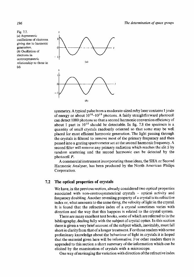
196 The determination of space groups
Fig. 7.7.(a) Asymmetricoscillations of electronsgiving rise to harmonicgeneration.(b) Oscillation ofelectrons incentrosymmetricrelationship to those in(a).
- 1 -
- 1
(b)
symmetry. A typical pulse from a moderate-sized ruby laser contains 1 jouleof energy or about 1018-1019 photons. A fairly straightforward photocellcan detect 1000 photons so that a second harmonic conversion efficiency ofabout 1 part in 1015 should be detectable. In fig. 7.8 the specimen is aquantity of small crystals randomly oriented so that some may be wellplaced for most efficient harmonic generation. The light passing throughthe crystals is filtered to remove most of the primary frequency and thenpassed into a grating spectrometer set at the second harmonic frequency. Asecond filter will remove any primary radiation which reaches the slit S byrandom scattering and the second harmonic can be detected by thephotocell P.
A commercial instrument incorporating these ideas, the SHA or SecondHarmonic Analyser, has been produced by the North American PhilipsCorporation.
7.2 The optical properties of crystals
We have, in the previous section, already considered two optical propertiesassociated with non-centrosymmetrical crystals - optical activity andfrequency doubling. Another revealing property of a crystal is its refractiveindex or, what amounts to the same thing, the velocity of light in the crystal.It is found that the refractive index of a crystal sometimes varies withdirection and the way that this happens is related to the crystal system.
There are many excellent text books, some of which are referred to in thebibliography, dealing fully with the subject of crystal optics. In this sectionthere is given a very brief account of the subject which, inevitably, must fallshort in clarity from that of a longer treatment. For those readers with somepreliminary knowledge about the behaviour of light in crystals it is hopedthat the material given here will be informative. For other readers there isappended to this section a short summary of the information which can beelicited by the examination of crystals with a microscope.
One way of envisaging the variation with direction of the refractive index

7.2 The optical properties of crystals 197
Fig. 7.8.Harmonic-generationdetector.
Kilter
Laser Crystals
Gratingspectrometer
of a crystal is to consider a point source of light within the material and tonote the limits of the disturbance after some time T. For an isotropicmaterial such as glass the disturbance will, as one would expect, extend outto a spherical surface. All points on this surface will act as a new source oflight and so the wave front spreads out preserving its spherical symmetry.
It is found that a crystal belonging to the cubic system behaves in asimilar way. The cubic symmetry implies that any physical properties ofthe crystal are identical in the three mutually orthogonal directions alongthe axes. In addition the properties in sets of directions related by the triador tetrad axes would also have to be identical; if the surface of thedisturbance was not a sphere it would have to be something else havingcubic symmetry.
The next type of crystal we shall consider is the uniaxial crystal which is acrystal having a unique axis and belonging to the trigonal, tetragonal orhexagonal systems. The light from a point source within such a crystal willbe found to split into two components which are polarized at right angles toeach other and which in general have different refractive indices. Theray-velocity (or wave) surfaces may be of two types which are shown in oneoctant of a set of cartesian axes in fig. 7.9(a) and the planes through thesurfaces containing the unique axis are shown in fig. 1.9(b). The followingpoints will be noted:
(i) One of the wave surfaces is spherical while the other is an oblatespheroid (negative uniaxial crystal) or a prolate spheroid (positiveuniaxial crystal). A spheroid is an ellipsoid with two equal axes and inthis case the equal axes are perpendicular to the unique axis so that thespheroid has circular sections perpendicular to the unique axis. Theaxis of the spheroid along the unique axis equals the radius of thespherical surface.
(ii) The surface has been called a ray-velocity (or wave) surface and this isnot to be confused with a wave front which is a surface of constant phasemoving through the crystal. If we consider a plane wave front, 00'O",moving through the medium, as in fig. 7.10, then it is possible todetermine, by Huygens' construction, the new position of the wavefront, PP'P", after a time AT. Thus it would be possible to interpret the

198
Fig. 7.9.(a) Ray surfaces ofuniaxial crystals. Thestriations indicate theelectric-vector direction.
The determination of space groups
[a]
spheroidal wave surface as the envelope of the wave fronts movingoutwards in various directions in the crystal as is shown in fig. 7.11.
(iii) The striations which define the surfaces in fig. 1.9(a) also indicate thedirections of the electric vector for the plane wave moving in theappropriate direction in the crystal. Thus in fig. 7.12 the initial un-polarized wave front, 00', whose normal is in the direction OP is splitinto two components, PP' and QQ\ moving at different velocities andwith their electric vectors in the directions shown. It will be noted thatthe unique axis is also a direction in which a plane wave of any state ofpolarization (or unpolarized) will always move with the same velocityand for this reason it is termed the optic axis of the crystal. It must be
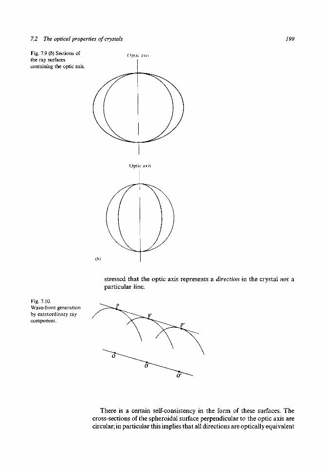
7.2 The optical properties of crystals
Fig. 7.9 (b) Sections ofthe ray surfacescontaining the optic axis.
799
Optic axis
(h)
stressed that the optic axis represents a direction in the crystal not aparticular line.
Fig. 7.10.Wave-front generationby extraordinary raycomponent.
There is a certain self-consistency in the form of these surfaces. Thecross-sections of the spheroidal surface perpendicular to the optic axis arecircular; in particular this implies that all directions are optically equivalent

200 The determination of space groups
Fig. 7.11.Ray front as envelopeof wave fronts.
Fig. 7.12.Generation of wavefronts and direction ofelectric vectors for thetwo components in auniaxial crystal.
perpendicular to the optic axis. For trigonal, tetragonal or hexagonalsymmetry one would expect sets of directions related by these symmetriesto be equivalent and hence it can be seen that if the surface is to be any sortof ellipsoid at all it has to be a spheroid. Again, if one looks at the sphericalsurface one sees that the electric-vector directions are all perpendicular tothe optic axis, and hence optically equivalent, no matter in which directionin space the light travels.
Direction of optic axis
Direction ofelectric vector
Electric vector perpendicularto plane of figure
One of the properties shown by uniaxial crystals is double refraction. Thiscan be seen if one looks at a small spot on a piece of paper through aparallel-sided slab of calcite. Two images of the spot are seen - one whereexpected along the normal to the slab but the other displaced from thenormal. A piece of Polaroid held above the slab and rotated extinguishes thespot images in turn at positions separated by TI/2, showing that the lightforming each of the images is plane-polarized and that the planes ofpolarization are perpendicular to each other. If the calcite slab is rotated as

7.2 The optical properties of crystals 201
Fig. 7.13.(a) Path of extraordinaryimage when crystalrotates.(b) Production ofordinary andextraordinary images ina uniaxial crystal.
illustrated in fig. 7.13(a) then the expected image, 0, does not move whereasthe unexpected one, E, rotates about 0. The reason for this behaviour may befollowed in fig. 7.13(b) which shows a principal section of the calcite slab, thatis to say, a section containing the optic axis, which is also perpendicular to thesurface of the slab. A plane wave front 00' falls normally on the surface and itcan be seen that it is split into two plane waves, one moving normal to thesurface and the other at some angle to the normal. This latter wave front is notnormal to its direction of motion. The wave front is a surface of constantphase while the direction of motion of the light is the direction in which theenergy moves and these need not be perpendicular to each other. Howeverthe electric vector is always in the plane of the wave front or is tangential to it ifthe wave front is not planar. The rays and waves which behave like those in anisotropic medium and give rise to the image 0 are called the ordinary rays andwaves; the others are called extraordinary rays and waves.
An experiment which clearly identifies a uniaxial crystal is to examine itin convergent light between crossed Polaroids (or other devices forproducing plane-polarized light). The experimental arrangement is shownschematically in fig. 7.14(a); light from an extended source S passes through
Path of Ewhen crystal
rotates
(a)
Extraordinary wave front
Ordinary wave front
\ 4
O'
(b)

202
Fig. 7.14.(a) Experimentalarrangement forobserving a crystal indivergent light.(b) Cone of light ofsemi-angle 9 entering thepoint 0 of a crystal.(c) The division of thecone of light into twocomponents.(d) The relativeamplitudes anddirections of thecomponents for variousrays in the cone.
The determination of space groups
A
Viewingsystem
(b)- t -
(c)
Ordinarycomponent
Extraordinarycomponent
(d)

72 The optical properties of crystals 203
a polarizer P and a lens L so that, at all points of the crystal, light passesthrough for a whole range of angles contained within a fairly wide-anglecone. After passing through the crystal and a crossed Polaroid analyser Athe light is viewed by what amounts to a telescope focussed at infinity sothat what is seen at any point of the field of view is representative of the lightpassing in some direction through the crystal over the whole of its area.
In fig. 7A4(b) there is represented a cone of light passing in at the point 0of the crystal and making an angle 6 with the optic axis which is hereassumed to be normal to the crystal face. The direction of the electric vectorfor light passing through P is shown by the striations and this is also shownby the double-headed arrows at the base of the cone. Within the crystal theoriginal cone will split up into two separate cones corresponding to the twowave surfaces in a uniaxial crystal but once they emerge from the crystalthey will again each form a cone of semi-angle 6. This is shown in fig. 7.14(c);the relative displacement of the two emergent cones will, in practice, be verysmall.
We now consider the separation of the original cone into the separatecones. In fig. 7.14(d) we look at the situation in (b) straight down the opticaxis and we also show the striations corresponding to the wave surfaces infig. 1.9(a). The circles correspond to striations on the sphere, the ordinarywave surface, and the radial lines to striations on the spheroid, theextraordinary wave surface. It is clear from (d) that a ray passing throughthe point B of the cone produces only an extraordinary ray in the crystalsince there is no component of the electric vector in the direction of thecircular striations. When this ray reaches the crossed Polaroid analyser A itwill be completely absorbed and so no light gets through the system in adirection corresponding to B. Similarly a ray passing through the point F ofthe cone produces only an ordinary ray and again is blocked by theanalyser. It should be noticed that this conclusion for the points B and F(also B' and F') is independent of 6 and so this produces in the field of view adark cross as is shown in fig. 7.15.
If, on the other hand, the direction of the light corresponds to the point Dwhere OD makes an angle it/4 with OB then two components pass throughthe crystal which are of equal magnitude. It can be seen in fig. 7.14(c) thatthere will be a phase difference between the components introduced bypassage through the crystal given by
(7.3)
Fig. 7.15.Appearance of uniaxialcrystal in convergentlight between crossedPolaroids with optic axisperpendicular to crystalface.

204 The determination of space groups
Fig. 7.16.Resultant of adding twoperpendicularlyplane-polarized beams oflight with various phasedifferences.
where \i and // are the refractive indices for the two polarization directionsand i is assumed to be the same for both rays. It is clear that as i increases fromzero so </> monotonically increases from zero (ft = // when i = 0). We can seein fig. 7.16 how the two components recombine for various values of (j>between 0 and In. When <j> is a multiple of 2n the recombined beams give aresultant equivalent to that entering the crystal - and this cannot go throughthe crossed Polaroid A. This gives a dark point in the field of view. For otherray directions, with the same value of 6 but given by C and E on either side ofD, the two components in the crystal are unequal in intensity and one doesnot get complete blackness when 0 is a multiple of 2n. The complete resultantfield of view is shown in fig. 7.15 and when this is seen it denotes a uniaxialcrystal. We have assumed that the light is monochromatic and that oneobtains only patterns of light and dark regions. If white light is used then thecondition for blackness in the field of view varies with the wavelength and theresult is a series of coloured rings although the dark cross is retained.
Directions ofpolarization of
components passingthrough the crystal
Resultantwhen cf) =
Plane Circularlypolarized polarized
Planepolarized
2TT
Circularly Planepolarized polarized
If the crystal surface is parallel to the optic axis then the appearance of thefield under the same experimental conditions as in fig. 7.14{a) is shown in fig. 7.17.
Fig. 7.17.Appearance of uniaxialcrystal in convergentlight between crossedPolaroids with optic axiscontained in the crystalface.
Optic axis

7.2 The optical properties of crystals 205
Crystals belonging to the triclinic, monoclinic and orthorhombic systemsare known as biaxial crystals and their ray surfaces are much morecomplicated than those for uniaxial crystals; a typical ray surface is shownin fig. 7.18(a). The surface is represented in one octant of a set of rectangularCartesian axes and is completed by mirror reflection in each of the principalplanes. The striations represent the direction of the electric vector for aplane wave tangential to the surface at the point in question.
The surface characteristics can also be appreciated by their intersectionswith the principal planes which are shown in fig. 7.18(fc). In the XZ plane,for example, the curves of intersection are a circle and an ellipse. It can beseen that rays travelling out to the circular boundary all travel with thesame velocity and this is consistent with what is seen in fig. 7.18(a)- that theelectric-vector direction is equivalent for each of them and along the Ydirection. The same consistency will be found for the circular boundaries inthe X Y and YZ planes.
In the X Y plane the two curves cross over and so a ray moving in thedirection OP has the same velocity for any plane of polarization. This isevident from fig. 7.18(a) which shows that all directions of the electricvector occur at P. Biaxial crystals have two optic axes but they are not inthe directions OP and OP'. These latter are known as ray axes; on theother hand, the optic axes are directions in which there is a single phasevelocity and they are the normals to the common tangent planes to thetwo parts of the surface. The optic axes are shown as OQ and OQ' in fig.7.18(fc). This point is illustrated in fig. 7.19 where two points, O1 and O2,on a plane wave front are used as origin points for Huygens-type waveletsto construct a new position of the wave front. It can clearly be seen that ifthe wave front is parallel to the common tangent plane to the two parts ofthe surface then there is only a single phase velocity. This definition of anoptic axis also applies to the uniaxial crystal for which the ray axis andoptic axis are identical.
If a biaxial crystal is used in the experimental arrangement of fig. 7.14then the resultant field of view shows the presence of the two optic axes. Ifthe crystal face is perpendicular to the bisector of the acute angle betweenthe optic axes then the appearance will take a symmetrical form dependenton the orientation of the polarizer to the line joining the optic axes. Twoexamples of these forms are shown in fig. 7.20.
Summary
1. In terms of crystal optics crystals can be divided into three types:(a) Cubic - these are isotropic in their optical properties and behave
optically like a non-crystalline material such as glass.(b) Uniaxial - these are crystals belonging to the trigonal, tetragonal
and hexagonal systems. Along the unique axis of the crystal, calledthe optic axis, the refractive index of light is independent of its state ofpolarization. For other directions light breaks up into two componentspolarized at right angles to each other and moving with differentvelocities.

Fig. 7.18.{a) Ray surfaces for a biaxial crystal.(b) Intersection of ray surfaces with principal planes of Cartesian axes.

7.2 The optical properties of crystals 207
Fig. 7.19.The optic axis is alongthe direction in whichboth rays have the samephase velocity. It isperpendicular to thecommon tangent surfaceto two parts of the raysurface.
Combined wave front
Fig. 7.20.Appearance of a biaxialcrystal in convergentlight between crossedPolaroids for twodifferent orientations ofthe crystal.
(c) Biaxial - these are crystals belonging to the triclinic, monoclinic ororthorhombic systems. There are two directions in which light of anypolarization moves with the same phase velocity. These are the twooptic axes of the crystal.
2. If a crystal is viewed in convergent light between crossed Polaroids as infig. 7.14(a) then one can usually distinguish which type of crystal one isdealing with. Some characteristic patterns are shown:(a) Fig. 7.15 - a uniaxial crystal with the optic axis normal to the crystal
face.(b) Fig. 7.17 - a uniaxial crystal with the optic axis contained in the
crystal face.(c) Fig. 7.20 - a biaxial crystal with the normal to the crystal face
bisecting the acute angle between the optic axes.Other forms of these patterns exist and can be recognized.

208 The determination of space groups
3. The orientation of the crystal can be determined by examination with amicroscope; identification and composition determination are alsopossible in some circumstances. An important characteristic of this typeof examination is that it is rapid and therefore well worth doing with anew and unknown crystal.
7.3 The symmetry of X-ray photographs
The very first type of X-ray diffraction photograph, the Laue picture, wasmade by diffracting white (non-monochromatic) X-rays from a stationarycrystal. For this type of arrangement one obtains a large number ofdiffraction spots - indeed, one should obtain almost a complete set ofdiffraction data. In fig. 7.21(a) there is depicted the crystal at 0 and areciprocal lattice point at P. For some X the sphere of reflection will passthrough P and with all wavelengths available diffraction may take place forany reciprocal-lattice point on the incident-beam side of the plane throughthe crystal perpendicular to the incident beam. All orders of the same set ofBragg planes will overlap with the spots produced by different wavelengths(see §5.10).
Fig. 7.21.(a) With X-ray beamdown triad axis threeequivalent points fall onsphere of reflectiontogether.(b) A Laue picture downa hexad axis.

7.3 The symmetry of X-ray photographs 209
The Laue photograph is particularly suited to detecting symmetry axes ifthe X-ray incident beam is directed along, or very close to, the symmetryaxis. In fig. 7.2\(a) the incident beam is directed along a trigonal axis so thatthere are two other reciprocal-lattice points P' and P" equivalent to P andrelated to it by the trigonal axis. It is evident that the value of X which givesthe reflection P will also give those corresponding to the symmetry-relatedones, P' and P". These will form an equilateral triangle of spots on the film,all of the same intensity. Even if the axis is slightly offset from the incidentbeam the trigonal symmetry will still be evident. The triangles of spots willnot be equilateral and they may vary slightly in intensity since they areproduced by different wavelengths but the overall evidence from the wholephotograph is usually unmistakable. A typical Laue photograph takendown a hexad axis is shown in fig. 7.21(6).
One can also detect on other kinds of X-ray photographs sets ofequivalent reflections (other than Fhkl and F^j) which give informationabout symmetry elements in the crystal. For example if a unit-cell axis, sayb, is a diad axis, a twofold screw axis or is perpendicular to a mirror plane then
\Fua\ = \Flia\ = \Fw\ = \FaT\. (7.4)
We can deduce this relationship from the basic structure-factor relationship,equation (3.41), by noting that for these symmetry elements there are pairsof atoms with related positions as follows:
diad axis (x, y, z); (x, y, z)screw diad axis (x, y, z); (x, \ + y, z)mirror plane (x, y, z); (x, y, z).
Thus with a diad axis
*m = I /;exp{27ii(/zx,. + ky, + lz)}
= I /;[exp{27u(foc,. + kyj + lz$ + exp{2ni(-hxj + ky-3 - /z,.)}]j = i
= £ 2^exp(27ii/cj;J.)cos{27i(/2xj + Izj)} (7.5)J=i
from which relationship (7.4) follows. The reader may confirm thatrelationship (7.4) also follows for the other two symmetry elements and alsofor any tetrad or hexad axis.
If an oscillation photograph is taken about a 2 or 2 x axis or about an axisperpendicular to a mirror plane then the photograph will have the zerolayer as a line of mirror symmetry. This will be seen in fig. 7.22 which showsthat the reciprocal-lattice points (hkl) and (hkl) cut through the sphere ofreflection simultaneously. When an oscillation photograph shows a mirrorline then it is certain that the space group is at least monoclinic and if mirrorlines are located about two different axes the symmetry must be at leastorthorhombic (a third axis giving a mirror line must also then be present).
The symmetry of the weighted reciprocal lattice, which can be obtainedfrom X-ray photographs, will reveal the presence of all the symmetry
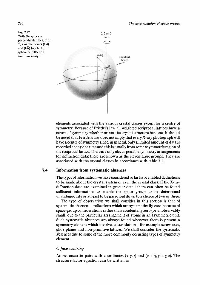
210 The determination of space groups
Fig. 7.22.With X-ray beamperpendicular to 2, 2 or2l axis the points (hkl)and (hlil) touch thesphere of reflectionsimultaneously. Incident
beam
elements associated with the various crystal classes except for a centre ofsymmetry. Because of Friedel's law all weighted reciprocal lattices have acentre of symmetry whether or not the crystal structure has one. It shouldbe noted that Friedel's law does not imply that every X-ray photograph willhave a centre of symmetry since, in general, only a limited amount of data isrecorded at any one time and this is usually from some asymmetric region ofthe reciprocal lattice. There are only eleven possible symmetry arrangementsfor diffraction data; these are known as the eleven Laue groups. They areassociated with the crystal classes in accordance with table 7.1.
7.4 Information from systematic absences
The types of information we have considered so far have enabled deductionsto be made about the crystal system or even the crystal class. If the X-raydiffraction data are examined in greater detail there can often be foundsufficient information to enable the space group to be determinedunambiguously or at least to be narrowed down to a choice of two or three.
The type of observation we shall consider in this section is that ofsystematic absences - reflections which are systematically zero because ofspace-group considerations rather than accidentally zero (or unobservablysmall) due to the particular arrangement of atoms in an asymmetric unit.Such systematic absences are always found whenever there is present asymmetry element which involves a translation - for example screw axes,glide planes and non-primitive lattices. We shall consider the systematicabsences due to some of the more commonly occurring types of symmetryelement.
C-face centring
Atoms occur in pairs with coordinates (x, y, z) and (x + \, y + , z). Thestructure-factor equation can be written as
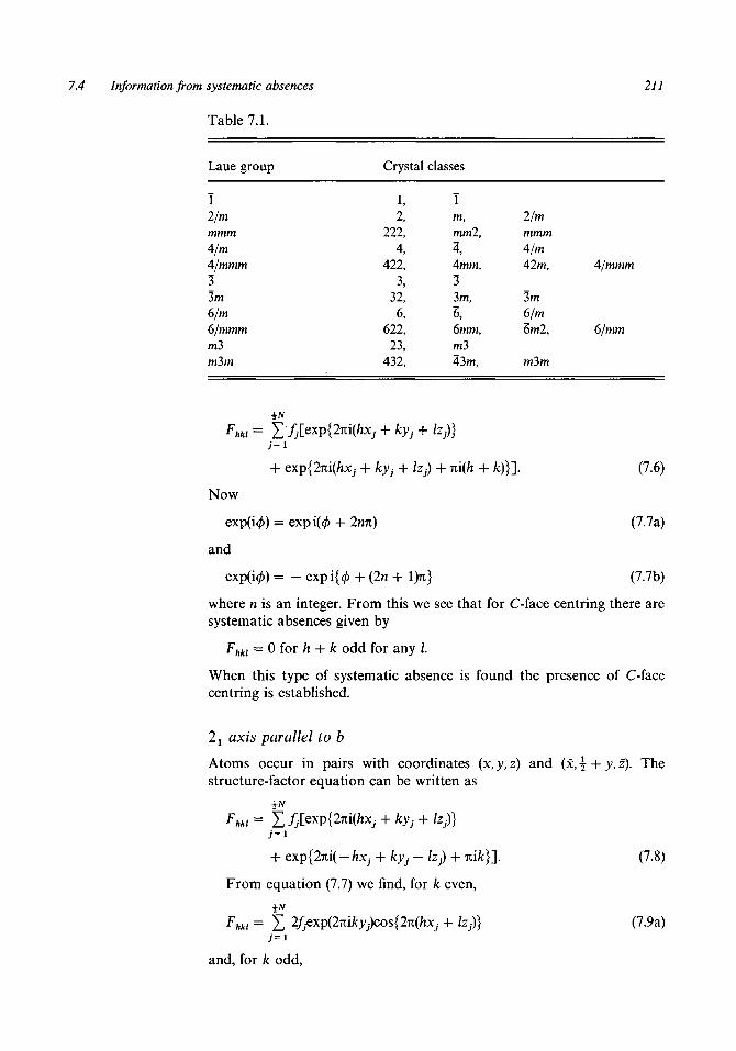
7.4 Information from systematic absences
Table 7.1.
211
Laue group Crystal classes
12/mmmm4/m4/mmm33m6/m6/mmmm3mbm
1,2,
222,4,
422,3,
32,6,
622,23,
432,
1m,mm2,4,4mm,33m,6,6mm,m343m,
2/mmmm4/m42m,
3m6/m6m2,
m3m
4/mmm
6/mm
Now
and
+ ty +
exp{27ii(/ixi + kyj + /z,)
i</>) = exp i(0 + 2rm)
(2n
/c)}]. (7.6)
(7.7a)
(7.7b)
where n is an integer. From this we see that for C-face centring there aresystematic absences given by
Fhkl = 0 for h + k odd for any /.
When this type of systematic absence is found the presence of C-facecentring is established.
2X axis parallel to b
Atoms occur in pairs with coordinates (x, y, z) and (x, \ + y, z). Thestructure-factor equation can be written as
Fkki = I /)[exp{27ii(/zx,. + kyj + lZj)}
+ exp{27ti( — hxj + kyj — lZj) + Tii/c}].
From equation (7.7) we find, for k even,
Fhki = Z 2//exp(27ii/cj;j)cos{27i(/ixJ- 4- izj)}
and, for k odd,
(7.8)
(7.9a)
212 The determination of space groups
Fm = Z 2/jexp(27iifc^sin{2ii(/ixJ + Izj)} (7.9b)j= i
An examination of these expressions will show that the type ofsystematic absence which can occur is that
FOkO = 0 for k odd.
Whenever this systematic absence is found without others affectingreflections for which both h and / are not zero then the existence of a 2X axisparallel to b is established.
c-glide plane (perpendicular to b)
Atoms occur in pairs with coordinates (x, y, z) and (x, y,\-\- z). This gives,for / even,
Fhkl = Z 2ffixp{2ni(hxj + lzj)}cos(2nkyj) (7.10a)
and, for / odd,
Fm = £ 2ffxp{2ni(hxj + lzj)}sin(2nkyj). (7.10b)
The systematic absences which arise from these equations are that
Fhol = 0 for / odd.
This means that for the layer k = 0 only those reflections are observed for /even; if one had only these data available then one would judge that the c*spacing was twice as large as it really was or that the cell parameter wasone-half of its true value. The reason for this is that the (hOl) datacorresponds to that from a two-dimensional projection of the structuredown the y axis. The two-dimensional coordinates for this projection are(x, z) and (x, \ + z); if one breaks the projected cell into two by drawing theline z = \ then the two parts are equivalent. This is shown in fig. 7.23; in theprojection there is an effective unit cell with d = \c and this gives rise to thesystematic absences which are observed.
It should be noticed that a c-glide plane can only be diagnosed if a latticeabsence does not interfere. For example, for an A-face centred lattice
Fhkl = 0 for k + / odd for any h and, in particular, this givesFh0l = 0 for / odd for any h.
Thus the systematic absences due to the c-glide plane would be masked.There follows in table 7.2 a selection of some of the more common
lattices and symmetry elements and the systematic absences which followfrom them.
We shall now look at a few cases where systematic absences givespace-group information.
Case 1. Monoclinic. All reflections observed except 0/cO for k odd. The cellmust be primitive with a 2X axis along b. The space group is P21.

7.4 Information from systematic absences
Table 7.2.
213
Lattice
P
ABCF
I
Absences
None
k + / = 2n + 1/i + / = 2n + 1h + fc = 2rc + 1/i, /c, / not all odd
or all evenh + k + l = 2n + l
Symmetry element
2 j || to a axis2j || to b axis2± || to c axis
hOO for h = 2n + 10/cO for A; = 2w + 100/ for / = 2n + 1
Symmetry element
T, 3,4,6, ml2,3,4,6 Ja ± to b axisa _L to c axisfr ± to a axisfr J_ to c axisc _L to a axisc ± to b axisn l t o o axis«_L to b axis«_L to c axis
Absences
None
hOl for /i/z/cO for hOkl for fchkO for /c0/c/ for / =hOl for / =Okl for /cM)/ for hhkO for /i
= 2n= 2«
= 2n= 2«
= 2n-= 2n •
+ / =+ / =
+ 1+ 1+ 1+ 1
f 1f 12« + 12rc + 1
= 2n + 1
Fig. 7.23.Crystal projection downb axis perpendicular towhich there is a c-glideplane.
Case 2. Monoclinic. The observed absences are
hkl for h + k = 2n + 1.
The cell must be C-face centred but otherwise no other symmetry element isindicated by the systematic absences. However since the system is mono-clinic, there must be along one axis, say b, a 2 or 2 (= m) symmetry axis or both.
The possible space groups are C2, Cm or C2/m. A monoclinic cell with nosystematic absences would be P2, Pm or P2/m; the way of distinguishing

214 The determination of space groups
these is discussed in §7.6 and similar methods can be used for theface-centred cells.Case 3. Orthorhombic. The observed absences are for
/zOO with h odd0/cO with k odd00/ with / odd.
The cell is primitive with a 2X axis along each cell axis. The space group istherefore P212121.Case 4. Orthorhombic. The systematic absences are for
hklfovh + k + l = In + 1Ofcf for k = In + 1MM for / = In + 1hkO for h = 2n+L
The systematic absences tell us that the lattice is /-centred, that there is afo-glide plane perpendicular to the a axis, a oglide plane perpendicular tothe b axis and an a-glide plane perpendicular to the c axis. Hence the spacegroup is Ibca.
There is a diffraction phenomenon which can sometimes interfere withthe identification of symmetry elements from systematic absences. This is aprocess of double reflection where the beam reflected from one set of latticeplanes is reflected from another set of planes which happens to be in thecorrect orientation. The phenomenon was first pointed out by Renninger(1937) and the reflections so produced are called Renninger reflections.They occur when two reciprocal-lattice points touch the sphere of reflectionsimultaneously and their formation can be followed by reference to fig. 7.24.The incident beam CO falls on the crystal at O and produces a reflection inthe direction CO' due to the reciprocal-lattice point Of touching the sphereof reflection. The other reciprocal-lattice point P on the sphere of reflection
Fig. 7.24.Production of Renningerreflections.

7.5 Intensity statistics 215
corresponds to a systematic absence and so will not give rise to a reflectiondue to the incident beam CO.
Now let us assume that an incident beam falls on the crystal in thedirection CO'. We now centre the reciprocal lattice at 0' and it is clear fromthe figure that O'P corresponds to a reciprocal-lattice vector s3( = s2 — sx).Thus a reflection would be produced in the direction CP.
The reflected beam CO' due to the reciprocal-lattice vector sx can thus bereflected again, the beam leaving the crystal along CP, the direction of aforbidden reflection for the incident beam CO. If the intensities correspondingto the reciprocal-lattice vectors sx and s3 are both strong the Renningerreflection can be very prominent. Renninger reflections can usually berecognized by their very sharp, non-diffuse appearance; the double-reflectionprocess will happen only for a restricted range of wavelengths of thecharacteristic radiation being used. In practice if one has overwhelmingevidence of a given type of systematic absence with one or possibly two faintreflections disturbing the pattern then one should suspect that the systematicabsences are genuine and that Renninger reflections are occurring. Ofcourse if P was not a point corresponding to a systematic absence aRenninger reflection would still occur and this would enhance the intensityof the primary reflection and would appear as an experimental error in thedata.
7c5 Intensity statistics
None of the techniques we have previously considered, with the possibleexception of optical goniometry, has enabled a centre of symmetry to bepositively detected. In fact, as was shown by Wilson (1949), the presence orabsence of a centre of symmetry does impress itself on the diffraction databut in a way which does not reveal itself without a certain amount ofanalysis - through the distribution of the structure amplitudes or intensities.
In order to derive these distributions it will be necessary to use animportant theorem of statistical theory - the central-limit theorem. Thisstates that:
The sum of a large number of independent random variables will have anormal probability distribution with mean equal to the sum of the means ofthe independent variables and variance equal to the sum of their variances.'
Let us see what this means. We consider a number N of independentrandom variables Xj (j = 1 to N) which have means Xj and variances aj.There are no restrictions on the distribution functions of the variables x andthe distributions can all be different. The sum of the variables
(7.11)
has a mean
X = £ ^
and a variance

216 The determination of space groups
o2 = I a2. (7.13)
The probability distribution of X is given by the normal distribution
- (X - X)2/2<72} (7.14)
which means that the probability that the sum lies between X and X + dXis P(X)dX.
This theorem can now be applied to the distribution of the structurefactors for a centrosymmetric structure. The structure factor equation canbe written
where h is the reciprocal-lattice vector. However all the terms in thesummation are not independent because for an atom at r7- there is also oneat —Vj. The equation can be rewritten as the sum of a number ofindependent terms as
Fh= £ 2/}cos(27ih-r,.) (7.15)
where the summation is over one asymmetric unit. Comparing equation(7.15) with equation (7.11) it will be seen that we should equate 2fj cos(2iihTJ.)to Xj so that
Xj = 2fj cos(2uhTJ.) = 2fj cos(27ihT,-). (7.16)
If we assume a random distribution of atomic positions then all positions inthe unit cell are equally probable and
cos(27th-r,.) = 0 (7.17a)
and hence
x~j = 0. (7.17b)
The variance of x- is given by the well-known expression
OL] = X ~ 2 - XJ2. (7.18)
Since Xj = 0 then
a] = 4/? cos2(27thT;)
= 2/2 (7.19)
since the mean value of cos2 6 is 0.5.
Thus the mean value of the structure factor is given by
F=YJx~j = 0 (7.20)
and its variance is given by

7.5 Intensity statistics 217
(7.21)
The distribution function of F is now given by
(7.22)
The form of this function, the normal Gaussian curve, is shown in fig. 7.25. Itcan only be an approximation to the true distribution since we know that F
N
has a maximum possible value of £ fp whereas the Gaussian curve extends
from — oo to + oo. A more exact theory has been given by Klug (1958).Before looking at the properties of equation (7.22) any further to see how
one could use it to distinguish a centrosymmetric structure we shall firstfind the corresponding distribution for a non-centrosymmetric structure.For such a structure we have
= Awhere
= I/)C0S(27lhT,.)
The distributions of A and B can be found separately - thus
Fig. 7.25.The centric distributionfunction.

218 The determination of space groups
so that
P(A) = (7iE
and similarly
; - A2/X) (723a)
:(7iE)-"exp(-B2/Z). (7.23b)
Since A and B are the real and imaginary parts of the structure factor theycan be plotted on an Argand diagram. The probability that A lies between Aand A + dA, and also that B lies between B and B + d£, is given by
?(A)?(B)dA dB = (Tt1exp( - | F |2/S)dv4 dB. (7.24)
The region defined by the above probability is shown in fig. 7.26(a) andsince dAdB is an element of area in the diagram we can say that the
Fig. 7.26.(a) Region definedbetween A and A + dAand between B andB + dB for a complexstructure factor.(b) Region of complexspace for which structureamplitude is between | F |and | F | + d | F |.
Imaginary partoff
Real part
Imaginary partoff-
Real partoff
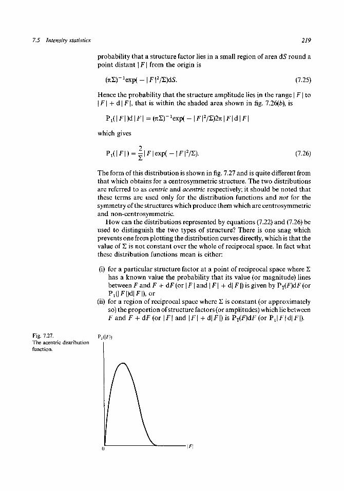
7.5 Intensity statistics 219
probability that a structure factor lies in a small region of area dS round apoint distant | F | from the origin is
Hence the probability that the structure amplitude lies in the range | F | to| F | + d | F |, that is within the shaded area shown in fig. 7.26(b), is
which gives
i> (7.26)
The form of this distribution is shown in fig. 7.27 and is quite different fromthat which obtains for a centrosymmetric structure. The two distributionsare referred to as centric and acentric respectively; it should be noted thatthese terms are used only for the distribution functions and not for thesymmetry of the structures which produce them which are centrosymmetricand non-centrosymmetric.
How can the distributions represented by equations (7.22) and (7.26) beused to distinguish the two types of structure? There is one snag whichprevents one from plotting the distribution curves directly, which is that thevalue of Z is not constant over the whole of reciprocal space. In fact whatthese distribution functions mean is either:
(i) for a particular structure factor at a point of reciprocal space where £has a known value the probability that its value (or magnitude) linesbetween F and F + dF (or | F | and | F | + d| F |) is given by Pj(F)dF (or
J(ii) for a region of reciprocal space where £ is constant (or approximately
so) the proportion of structure factors (or amplitudes) which lie betweenF <mdF + dF(or \F\ and | F | +d |F | ) is PT(F)dF (or P
Fig. 7.27.The acentric distributionfunction.

220 The determination of space groups
There is a quantity which enables one to distinguish the two types ofdistribution and is independent of Z and that is
M = = . (7.27)
For the centric distribution
|o (^J (7.28)and
\F\2= 2F2PT(F)dF = Z (7.29)12 - ,l — o o
so that
MT = - = 0.637. (7.30)71
For the acentric distribution
^^ icZ)* (7.31)o
and
f00
|F | 2 = \F\2?1(\F\)d\F\ = X (7.32)Jo
so that
Mx = ^ = 0.785. (7.33)
The two values given in equations (7.30) and (7.33) are sufficientlydifferent to give a discriminating test. As an example in fig. 7.28 there isshown one quadrant of a rectangular reciprocal-lattice net for the h = 0layer for dicyclopentadienyldi-iron tetracarbonyl (Mills, 1958) togetherwith the values of | F | and | F |2. In fact the space group can be unambiguouslydetermined as P2Jc, which is centrosymmetric, but we shall treat the Okldata as though the space group was completely unknown. Very often axialstructure factors, i.e. 0/cO, 00/, are atypical and are real even when theprojection is non-centrosymmetric and these will be ignored in determiningthe values of | F | and | F |2. In addition the structure factors at low sin 6values tend to be statistically unreliable (Wilson, 1949) and will not be usedfor sin 6 < 0.2. The net is divided by arcs of radii which increase by 0.1 insin 9 and within each annular region are counted the number of points,£ |F | and Z|F|2. These results are shown in table 7.3.
We now take overlapping regions covering the sinfl ranges 0.2-0.4,0.3-0.5, etc., and for each range determine | F \ and | F |2 and then the valueof M. This process is illustrated in table 7.4 and it will be seen that the valueof M seems to decrease with increasing sin 9. This is probably due to the

7.5 Intensity statistics 221
Table 7.3.
sin 6 range
0.2-0.30.3-0.40.4-0.50.5-0.60.6-0.70.7-0.80.8-0.90.9-1.0
No. of points
3689
12161118
nn60
1331811041301668449
I|F|2
1814384350272096209434341238267
Fig. 7.28.| F | and | F |2 for (0/c/)data ofdicyclopentadienyldi-irontetracarbonyl.
large number of unobserved reflections at high angles whose contribution,if measurable, would change substantially the values of | F | and IT7!2.However the average value of M is 0.612, giving a fairly clear indication thatthe projection is centrosymmetric

222 The determination of space groups
Table 7.4.
sin 6 range
0.2-0.40.3-0.50.4-0.60.5-0.70.6-0.80.7-0.90.8-1.0
No. ofpoints
9141721282729
I|F|
193314285234296250133
Z|F|2
5657887071234190552846721505
\F\
21.422.416.811.110.69.34.6
\F\2
62963441920019717352
M
0.7280.7910.6740.6160.5700.5000.407
In order to get meaningful values of M it was necessary to divide thereciprocal net into regions in which Z did not vary overmuch. Crystallo-graphers frequently find it convenient to use structure factors corrected forfall-off in 6 and the unitary structure factor is particularly useful (see §§ 8.7and 8.8). This is defined by
(7.34)
Since
and for a real structure factor
(7.35)
It is assumed in equation (7.34) that the fjS are the actual scatteringfactors for the atoms, including the temperature factor, and not thestationary-atom scattering factors one finds in the published tables.
If one writes
(7.36)
7 = 1
and expresses Fh in the form of a summation then equation (7.34) becomes
Uh = £ rtj exp(27iih-r,.). (7.37)
When the structure contains atoms of more than one type the quantitiesrip known as the unitary scattering factors, will vary with sin 0 since theratio of scattering factors for different atoms does not remain constant; inparticular the higher the atomic number the more tightly bound are theelectrons and the less rapid is the relative fall-off of/ However one usually

7.5 Intensity statistics 223
makes the assumption that the w/s are constant over the whole of reciprocalspace.
By analogy with what we have had previously, the distribution functionsof the unitary structure factor for centrosymmetric and non-centrosymmetricstructures, respectively, are
PT([/) = (27i£)-*exp( - U2/2s) (7.38)
and
Pi(l L/1) = -11/1 exp( - 11/ |2A) (7.39)
where
6 = £ n). (7.40)
For a structure with N equal atoms in the unit cell
and
-JU>-i? (7-42)In order to determine IPs from observed data we note from equations
(7.29) and (7.32) that for both the centric and acentric distributions we shallhave
\U\2 = s. (7.43)
The | U |2's can be obtained from the | F |2's by applying some factor </>which depends upon sin 6. We can determine this factor from the conditionthat, for an annular region in reciprocal space after the factor has beenapplied, \Uf = e.
Dicyclopentadienyldi-iron tetracarbonyl has two molecules ofFe2(CO)4(C5H5)2 in the unit cell. We shall ignore hydrogen since itcontributes negligibly to the scattering and we take/F e : / o : / c = 21:4:3 overthe whole range of sin 0 which gives nFe = 0.105, no = 0.020, nc = 0.015 ande = 0.0536.
In table 7.4 in the sin 6 range 0.2-0.4, corresponding approximately tosin 8 = 0.3, the value of | F |2 is 629. Hence the best estimate of the factor <f>which one should apply to | F |2's at sin 6 = 0.3 to convert them into | U |2'sis 0.0536/629. The values of <j) for the other values of sin 9 may be foundsimilarly. The factor J~§ applied to the | F |'s will give | U |'s and y/4> isshown plotted in fig. 7.29. A smooth curve is drawn as close to the points aspossible and the curve is extrapolated at both ends. From this curve a linearscale, also shown in fig. 7.29, can be prepared. If the point O of the scale ispivoted at the origin of the reciprocal lattice then the reading of the scale atthe reciprocal-lattice points gives the factor which changes | F | into \U\.
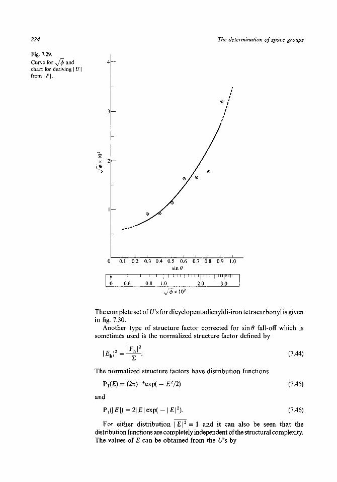
224 The determination of space groups
Fig. 7.29.
Curve for y/4> andchart for deriving | U \f rom|F | .
o
0 0.1 0.2 0.3 0.4 0.5 0.6 0.7 0.8 0.9 1.0sin0
0.6 0.8 1.0
i i I i i i i | i 1 1 i i i i i [ | i
2.0 3.0
The complete set of £/'s for dicyclopentadienyldi-iron tetracarbonyl is givenin fig. 7.30.
Another type of structure factor corrected for sin 6 fall-off which issometimes used is the normalized structure factor defined by
I F I 2
I2 - ' h 'l (7.44)
The normalized structure factors have distribution functions
and
(7.45)
(7.46)
For either distribution \E\2 = 1 and it can also be seen that thedistribution functions are completely independent of the structural complexity.The values of E can be obtained from the L/'s by
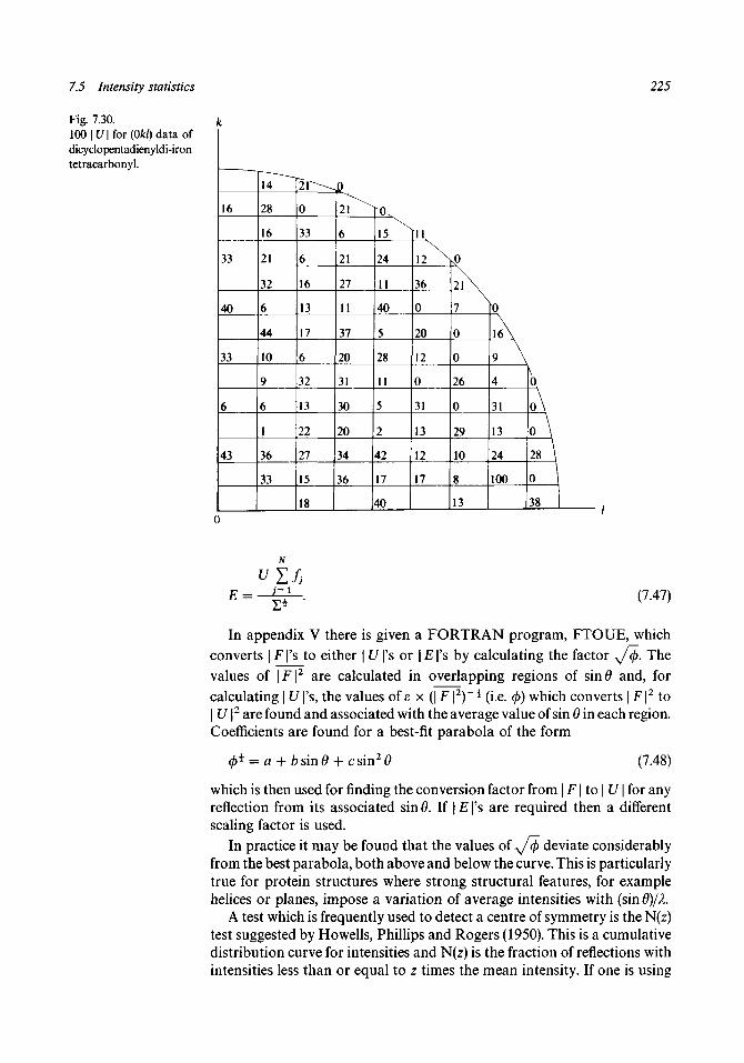
7.5 Intensity statistics 225
Fig. 7.30.100 | U | for (0/c/) data ofdicyclopentadienyldi-irontetracarbonyl.
k
.
16
33
40
33
6
43
I—-—^14
28
16
21
32
6
44
10
9
6
1
36
33
"21^^.
0
33
6
16
13
17
6
32
13
22
27
15
18
i>2 1 ^
6
21
27
11
37
20
31
30
20
34
36
ro.15
24
11
40
5
28
11
5
2
42
17
40
11
12 ^
36
0
20
12
0
31
13
12
17
K0
2l\
A0
0
26
0
29
10
8
13
to..\*\4
31
13
24
100
0
A•\"\0 |
38
(7.47)
In appendix V there is given a FORTRAN program, FTOUE, whichconverts | F |'s to either | U |'s or | E |'s by calculating the factor <v/$. Thevalues of \F\2 are calculated in overlapping regions of sin# and, forcalculating | U |'s, the values of £ x (| F | 2 )~* (i.e. (/>) which converts | F |2 to| U |2 are found and associated with the average value of sin 6 in each region.Coefficients are found for a best-fit parabola of the form
= a + b sin 9 + c sin2 6 (7.48)
which is then used for finding the conversion factor from | F | to | U | for anyreflection from its associated sin 6. If | E |'s are required then a differentscaling factor is used.
In practice it may be found that the values of y/ip deviate considerablyfrom the best parabola, both above and below the curve. This is particularlytrue for protein structures where strong structural features, for examplehelices or planes, impose a variation of average intensities with (sin 0)1 L
A test which is frequently used to detect a centre of symmetry is the N(z)test suggested by Howells, Phillips and Rogers (1950). This is a cumulativedistribution curve for intensities and N(z) is the fraction of reflections withintensities less than or equal to z times the mean intensity. If one is using

226 The determination of space groups
data with a sin 6 fall-off then one must always compare an intensity with thelocal average to determine the appropriate z. However if one has | U |'s or| £/|2's available then for any reflection
\U\2
z = ^ - U (7.49)£
It is straightforward to derive the theoretical forms of N(z) from PT(£/)and Px(| U |). For PT((7), N(z) is the proportion of IPs with values between
and — y/zs thus
Ni(z) = I Prfl/Jdl/ = erf( / | j (7.50)
where
is the well-tabulated error function. Similarly
Nt(z) = Pjd 1/ |)d| 1/1 = 1 - exp( - z). (7.51)Jo
These two functions are tabulated in table 7.5 and shown graphically infig. 7.31.
For dicyclopentadienyldi-iron tetracarbonyl the values of | U | corres-ponding to various values of z and the numbers of reflections with \U\2 lessthan ze are also shown in table 7.5 and N(z) is also plotted in fig. 7.31. It isclear from this that the projection is centrosymmetric.
The general quality of Nx(z) and NT(z) can be seen in the distributionsPx(| F |) and PTCF) plotted in figs. 7.27 and 7.25 where, in particular, it will benoticed that the centric distribution has a higher proportion of small Ks. Itwas shown by Lipson and Woolfson (1952) and by Rogers and Wilson(1953) that other types of distribution could occur when there weremolecules with non-crystallographic centres of symmetry in the unit cell. Infig. 7.31 is shown the N(z) curve for a hypercentric distribution which occurswhen there are in a unit cell two centrosymmetric molecules related by acrystallographic centre of symmetry (fig. 7.32). It will be noticed that the dis-tribution has an even higher proportion of small intensities than the centricone. The form of the distribution has been given by Lipson and Woolfson;one important property which it has, as have all other distributions, is that| F |2 = Z, so that the procedure described for determining IPs is still valid.
The various distribution functions described in this section depend onrandomness of the atomic positions. When there is a very heavy atom in theunit cell, equivalent to a non-statistical aggregation of scattering power, orwhen atoms are in special positions (§8.1), the distributions can departmarkedly from those which have been described. In such cases testsinvolving the moments of the distributions can be used (Foster &Hargreaves, 1963a, 1963b; Pradhan, Ghosh & Nigam, 1985).

7.6 Detection of mirror planes and diad axes
Table 7.5.
227
z
0.00.10.20.30.4
0.50.60.70.80.91.0
Nx(z)
0.000.090.180.260.330.390.45
0.500.550.590.63
NT(z)
0.000.250.350.420.470.520.56
0.600.630.660.68
\u\0.000.07
0.103
0.127
0.146
0.164
0.179
0.194
0.207
0.220
0.23!
1.00
For Fe2
No.
0253037424750
50535959
85
:(CO)4(C5H5)2
, < | F | N(z)
0.000.290.350.440.490.550.59
0.590.620.690.69
Fig. 7.31.The cumulativedistribution curves forthe followingdistributions: acentric(equation (7.51)); centric(equation (7.50)); andhypercentric (fromsymmetry shown in fig.7.32).
N(z)
1.0 -
Hypercentricx Centric
Acentric
0 0.1 0.2 0.3 0.4 0.5 0.6 0.7 0.8 0.9 1.0
7.6 Detection of mirror planes and diad axes
The only common symmetry elements for which detection techniques usingdiffraction data have not been described are the diad axis and the mirrorplane. In fact one frequently needs to distinguish these two. For example,the space group of a monoclinic structure with no systematic absences isone of P2, Pm or P2/m. The last of these is centrosymmetric and cantherefore be isolated by an N(z) test but, if the test indicated a non-centrosymmetric structure, one would still be left with the choice of P2 or Pm.
It can be shown that when there is a mirror plane, perpendicular to the b

228
Fig. 7.32.Structure for whichcentrosymmetricalgroups are related by acentre of symmetry; thisgives rise to thehypercentricdistribution.
The determination of space groups
axis let us say, then the value of | F \h0l |2 is 2Z or twice the average value for
general reflection intensities. For a mirror plane atoms occur in pairs withcoordinates (x, y, z) and (x, y, z) and the structure factor equation become
Fhki = Z 2fj7 = 1
= Ahh iBhhl. (7.52)
Since Ahkl = Bhkl = 0 we have A\kl equal to the variance of Ahkl which, bythe central-limit theorem, gives
7 = 1
Zj} x cos2(27i/cy7)
Similarly B^kl = ^Z and hence
However for k = 0
(7.53)
2 x COS2{2TI(/ZX,. = 2 =
and
|2 _ B2hOl = 2 1 . (7.54)
Another, and easier, way of deducing this relationship is to see that thefc-axis projection will show complete overlap of pairs of atoms due to the

Problems to Chapter 7 229
mirror plane. Thus, in projection, there are \N double-weight atoms andthe effective value of Z, Zm, becomes
I 2 = 22. (7.55)
In a similar way the presence of a diad axis along b shows itself in that| FokO |2 is TL. Pairs of atoms are related with coordinates (x, y, z) and (x, y, z)so that projected on to the b axis they overlap at (0, y, 0). Since, in general,there are fewer reflections involved this test for a diad axis is normally lessreliable than that for a mirror plane.
In order to apply these tests all the observed data must be on the samerelative scale and the method of achieving this is described in § 9.2. It is alsonecessary to compare the values of | F |2 for similar narrow ranges of sin 9and not for all the data together, since 2 will not have the same average overthe whole three-dimensional reciprocal lattice as it has for a one- or two-dimensional projection.
Problems to Chapter 7
7.1 What systematic absences are given by the following symmetry elements?(a) /-centred lattice,(b) n-glide plane perpendicular to b,(c) 3X axis.
7.2 Identify the space groups given by the following sets of systematicabsences:(a) Primitive monoclinic lattice:
0/cO only present for k = 2n,hOl only present for / = In.
(b) Primitive orthorhombic lattice:Okl only present for k + / = 2n,hOl only present for h = In,hOO only present for h = 2n,0/cO only present for k = 2n,00/ only present for / = In.
7.3 In table 7.6 are given the (hOl) and (Okl) data for m-toluidinedihydrochloride (Fowweather & Hargreaves, 1950). By comparingintensities with the local averages, determine N(z) for each projectionand determine whether they are centrosymmetrical or non-centrosym-metrical. The data are given in order of sin 6 and hence may be taken inoverlapping groups of consecutive items.
7.4 Using the output file generated in the solution of Problem 3.4, use theprogram FTOUE to find the normalized structure factors (| E |'s) for the(hOl) reflections of the phenylethylammonium salt of fosfomycin. Plotthe values of /^ found by averaging in sin 9 regions and compare withthe curve given by equation (7.48). You may request output of thevalues of a, b and c (equation (7.48)) when running FTOUE.

^.-H
^H
^^
CS
JfN
)^^
-,
osO o
o c
oo vo
3 Oo
fN
fN
O
fN ~*
o o
CO fN
CN *•*
CO SO
O O
so
CN
Oo
fNfN
r^ r^ *"
o o o
ON
»/O
OsoOo
SO
fN
r-o
fNot—.
o
fN
CO
O
so
SO
O
OO
fN
ON O
O O
CNO
sor-o
OO OO
fN '—i
fN so
o o
ON r~
fN fN
~H CO
o o
o
CN
O
SO
CN
O
ON
C
N
OO
<
^-t O
—
i CN
so O
N
so OO
rn -T
<N(N
O
'•~ co" ©
<N
'
*—i
CN
O
CO
r}- CNIO
-H
T
f SO
> o
o o
o o
o o
o o
o o
o o" o
o
o" o
o* o
©" o
o" ©" ©" o o
o ©" o
©" o" ©"
o" o o" o" o" o" o"
rsf O*
"^ v
^ \^ |r*~T
ITJ^ "o o~o o
g o
g g
o^g g o^o^g g
o^o^o^o^g o-o^ISO
|co so
ISO
ITJ-
so ISO
IVJ CO
ISO so
"t I'—
> <O
^^
so <
I^
^ f^
f^ ^
^ f^
f^ f^
f*
f^ ^
^ f"
f^
f"
^
en" o"
; o o
o o
o
gg
g g
gg
gg
CO
ON
ON
O
OO
^
oo »/~
>O
TH (N
«
O co co O
'
^^
^c
oc
os
ou
oc
no
or
ro
cN
cN
o<
^T
tOOOOOOOOOOOOO-OOO
H
« H
«
O
H «
O
H
-^ fS
I(N
(N
O H
IN
(N

8 The determination of crystal structures
8.1 Trial-and-error methods
The object of a crystal-structure determination is to locate the atomicpositions within the unit cell and thus completely to define the wholestructure. Sometimes there are special features in the diffraction pattern, thespace group or the suspected chemical configuration of the material underinvestigation which enable a guess to be made of the crystal structure or atleast restrict it to a small number of possibilities. In the early days of thesubject, when methods of structure determination were poorly developed,only the simpler types of structure could be tackled and trial-and-errormethods based on such special features were commonly used. That is not tosay that such techniques are now outmoded - no crystallographer wouldignore the information from special features if it was available, but he doesnot rely on such information as much as hitherto.
One type of situation which is of great importance and is always sought bythe crystallographer is when space-group considerations lead to the fixing orrestricting of the positions of atoms or whole groups of atoms. If acentrosymmetric unit cell has only one atom of a particular species (or an oddnumber) then that atom (or one of them) must be at a centre of symmetry. In acase with an odd number of atoms in a cell with a diad axis one of the atomswould have to lie on the diad axis. Similarly, in some situations, an SO4 groupmay have to be symmetrically arranged on a triad axis as shown in fig. 8.1. It isalso possible to gain stereochemical information from space-grouprequirements so that a molecule may be found necessarily to have a centre ofsymmetry or a diad axis of symmetry within itself.
An interesting example of a structure determination using this sort ofinformation is provided by the hydrocarbon fluorene, a molecule of whichis shown in fig. 8.2. This was solved by Brown and Bortner (1954) whoseX-ray data showed the crystal system to be orthorhombic, of space groupPna21 or Pnam with four molecules per unit cell. The unit-cell dimensionswere a = 8.50, b = 5.71 and c = 19.00 A. Subsidiary evidence showed thatthe space group was probably Pnam for which in general there are eightsymmetry-related positions. The only way in which four fluorene moleculescan be accommodated in the cell is if the molecule itself has a mirror planewhich coincides with the crystallographic mirror plane. This could meaneither that the molecule is precisely planar and lies completely in the mirrorplane or that the line AB in fig. 8.2 is a mirror plane for the molecule. Thelatter alternative was considered the more likely and, if the molecular shapewas assumed to be known - approximately at any rate - then the crystalstructure could be defined in terms of three parameters. These could be the
231

232
Fig. 8.1.An SO4 group arrangedon a triad axis.
The determination of crystal structures
Fig. 8.2.An outline of the carbonatoms of fluorene.
x and y coordinates of the point A and the angle made by the line AB withthe y axis. For the a ox b axis projections there are only two parameters.Structure factors were calculated for various positions of the modelmolecule and reasonable agreement of calculated and observed (hOI) and(O/cZ) structure factors was found for the point A at position (0.353, 0.431,0.250) with AB making an angle 30.5° with the y axis.
As a measure of agreement between observed and calculated structurefactors crystallographers use a quantity called the reliability index orresidual defined by
(8.1)
The Fo's and Fc's are the observed and calculated structure factorsrespectively and, of course, for them to be comparable the Fc's must includethe temperature factor. The way that one can determine the temperaturefactor from the observed data is described in § 9.2.

8.2 The Patterson function 233
Once a trial structure has been found which is close enough to the truestructure to give a low value of R then one can refine the structure by theroutine procedures which are described in chapter 9. The whole crystal-structure problem consists of getting the first trial structure; once thecrystallographer has his foot in the door, so to speak, the crystal structure isall but solved.
If there are a few very strong reflections with high unitary structurefactors then these alone can reveal the structure, particularly if one hassome initial idea of the stereochemistry of the substance under investigation.For a centrosymmetric structure, if a particular | Uh | is very large, then theatoms will tend to have coordinates r such that cos(27th*r) is either near +1for each of them or near — 1. One can try various combinations of signs forthe few structure factors and, in two dimensions, lines can be drawncorresponding to cos(27th*r) = ± 1 depending on which sign is being tried.In fig. S3(a) there is shown a diagram given by Dunitz (1949) demonstratinghow six strong reflections revealed the position of the molecule in the fo-axisprojection of 1,2,3,4-tetraphenylcyclobutane. The sets of lines correspondingto cos{2n(hx + lz)} = ± 1 are shown, the sign taken in each case beingindicated in the diagram. To show how well this indicated the correctposition, the final electron-density map is shown in fig. 8.3(fc). Anotherexample in which information was gained from only one very strong re-flection is shown in fig. 8.3(c) where it can be seen that in the fo-axisprojection of para-nitroaniline (Abrahams & Robertson, 1948), all theatoms lie along the direction of the (202) planes, where the (202) reflection isthe one which is very strong.
When the structure is a molecular one then the shape of the unit cell andthe restrictions on location imposed by symmetry elements may enable atrial structure to be found from packing considerations alone. The separatemolecules may be linked by hydrogen bonds or may have to be separatedby van der Waals distances. It can occasionally be very profitable to playabout with wire models of the unit cell and of the molecules. A computercan also be used systematically to explore various methods of packing toachieve sensible intermolecular distances and structure-factor agreement(Milledge, 1962).
A word of warning should be given about pseudo-symmetry arising as aresult of statistical disorder. This occurs when the structure consists of'unitcells' in which the atoms are arranged in two or more possible ways andwhere the arrangement from cell to cell varies randomly. Such a statistical-disorder situation is illustrated in two dimensions in fig. 8.4. The intensitiesof the Bragg peaks will correspond very closely to those from a 50:50 mixedstructure and there will be an apparent centre of symmetry. However onewould know from packing considerations that the two arrangements ofatoms could not occur simultaneously in one cell and this would also berevealed by the electron-density peaks which would be half the normal height.
8.2 The Patterson function
We have seen that the lack of knowledge of the phases of structure factorsprevents us from directly computing an electron-density map and so

( + J401
Fig. 8.3.{a) The six strong reflections which showed the 6-axis projection of 1,2,3,4-tetraphenylcyclobutane.(b) The 6-axis projected electron-density map for 1,2,3,4-tetraphenylcyclobutane (both {a) and (b) from Dunitz, 1949).(c) The /?-axis projection of p-nitroaniline showing the molecule lying along the (202) direction (from Abrahams & Robertson, 1948).
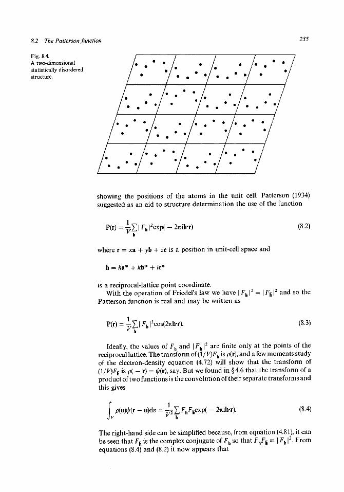
8.2 The Patterson Junction 235
Fig. 8.4.A two-dimensionalstatistically disorderedstructure.
showing the positions of the atoms in the unit cell. Patterson (1934)suggested as an aid to structure determination the use of the function
(8.2)
where r = xa + yb + zc is a position in unit-cell space and
h = ha* + /eb* + Zc*
is a reciprocal-lattice point coordinate.With the operation of Friedel's law we have | Fh \
2 = | Ffi |2 and so the
Patterson function is real and may be written as
1= -£|Fh|2cos(27ih-r).
V(8.3)
Ideally, the values of Fh and \Fh\2 are finite only at the points of the
reciprocal lattice. The transform of (l/F)Fh is p(r), and a few moments studyof the electron-density equation (4.72) will show that the transform of(1 /F)^ is p( - r) = I//(Y), say. But we found in §4.6 that the transform of aproduct of two functions is the convolution of their separate transforms andthis gives
p(i#(r - u)dt> = -r^Iv v h
~ 27iih-r). (8.4)
The right-hand side can be simplified because, from equation (4.81), it canbe seen that FH is the complex conjugate of Fh so that FhFH = | Fh |
2. Fromequations (8.4) and (8.2) it now appears that
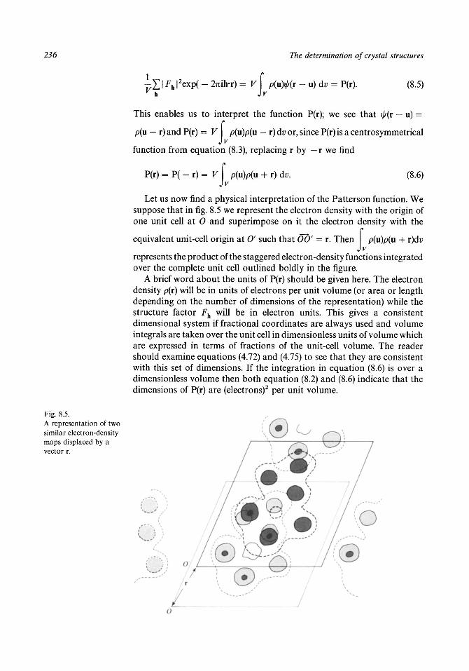
236
l ' e x P( - 2™h*r) = V I P(u)<A(r - u) di; = P(r).Jv
The determination of crystal structures
(8.5)
This enables us to interpret the function P(r); we see that ^(r — u) =
p(u — r) and P(r) = V p(u)p(u — r) dt? or, since P(r) is a centrosymmetricalJv
function from equation (8.3), replacing r by — r we find
P(r) = P( - r) = V\ p(u)p(u + r) dv.)v
(8.6)
Let us now find a physical interpretation of the Patterson function. Wesuppose that in fig. 8.5 we represent the electron density with the origin ofone unit cell at 0 and superimpose on it the electron density with the
equivalent unit-cell origin at O' such that 00' = r. Then p(u)p(u + r)duJv
represents the product of the staggered electron-density functions integratedover the complete unit cell outlined boldly in the figure.
A brief word about the units of P(r) should be given here. The electrondensity p(r) will be in units of electrons per unit volume (or area or lengthdepending on the number of dimensions of the representation) while thestructure factor Fh will be in electron units. This gives a consistentdimensional system if fractional coordinates are always used and volumeintegrals are taken over the unit cell in dimensionless units of volume whichare expressed in terms of fractions of the unit-cell volume. The readershould examine equations (4.72) and (4.75) to see that they are consistentwith this set of dimensions. If the integration in equation (8.6) is over adimensionless volume then both equation (8.2) and (8.6) indicate that thedimensions of P(r) are (electrons)2 per unit volume.
Fig. 8.5.A representation of twosimilar electron-densitymaps displaced by avector r.
1 (£),-

8.2 The Patterson function 237
What should the Patterson function P(r) show? Clearly it will be large ifstrong regions of electron density overlap in the displaced electron-densitymaps illustrated in fig. 8.5. In fact this is equivalent to saying that the valueof P(r) will be large if strong regions of electron density are separated by avector r in the unit cell. If there are several strong regions of electron densityseparated by the vector r the P(r) will show the total effect of this and willconsequently have a large value.
A well-resolved electron-density map shows regions of isolated electrondensity symmetrically disposed about the atomic centres. The contributionto the Patterson function of two atoms separated by a vector r will be adiffuse peak centred on r. In fig. 8.6(a) there are seen two atomic peaks of aone-dimensional electron-density map. When two such maps are overlappedwith a displacement r the value of P(r), as given by equation (8.6), dependson the product of the p's over the range for which they are non-zero. Thiswill be the integrated product for the shaded region in fig. 8.6(fc). Anexamination of this figure should make it clear that the maximumintegrated product will occur when the atomic centres exactly overlap andthat the width of a Patterson peak will be wider than that of anelectron-density peak.
The Patterson function will be a superposition of peaks derived from allthe pairs of atoms in the unit cell; if there was no overlap of Patterson peaks,or the overlap was slight, then the function P(r) would show the positions ofall the interatomic vectors in the cell. In fact the resolution of Pattersonmaps is usually rather poor and this is what should be expected. The Npeaks in an electron-density map, which will be well resolved, give rise toN(N — 1) vectors (ignoring the null vectors of an atomic position to itself)and the corresponding Patterson peaks are more diffuse than the electron-density peaks.
Thus if there is a set of atoms in positions r,- (j = 1 to N) they will give riseto a set of Patterson peaks at positions rt — r, for i = 1 to N and; = 1 to N.The N null vectors give a large peak at the origin, which can be seen fromequation (8.3), since
(8.7)
Fig. 8.6.(a) Two peaks ofelectron density.(b) Overlap of peakswhen twoelectron-density mapsare displaced by a vector
(a)
(M

238 The determination of crystal structures
The other vectors occur in centrosymmetric pairs r, — r,- and r,. — i\, againin conformity with the centrosymmetric nature of P(r) as shown byequation (8.3).
In the event that the structure is centrosymmetrical there is a systematicoverlap of some peaks to give double-weight peaks. For atoms withcoordinates ri9 —rt, xj and — r,. the interatomic vectors, apart from the nullvectors, are
r i ~~ (~~ r i ) r i — rj r i ~ ( ~ Tj)
r'j-h rj-i-rj r) - ( - r)-r,-r,. -r,-(-r,.) -Tj-ij
or, to summarize, single peaks at + 2rf, ± 2r;. and double peaks at ± (r • — r7)and ±(rt + r^).
Despite the overcrowded nature of Patterson maps useful informationcan frequently be derived from them and, indeed, quite complex crystalstructures can be solved from an interpretation of the Patterson function.Some common situations which occur and give rise to recognizablePatterson-map features will now be considered.
(i) Peaks due to heavy atoms
If there are a few atoms (perhaps only two) which have a higher atomicnumber than the remainder then the peaks due to these may well stand outin the ruck of minor peaks and give clear interatomic vectors. The totalPatterson density associated with a vector between two atoms of atomicnumbers Z{ and Z} is equal to Z{Z-, thus if a structure contains carbonatoms (Z = 6) and chlorine atoms (Z = 17) the types of peaks present andtheir weights are
C—C weight 36C—Cl weight 102
Cl—Cl weight 289.
In fig. 8.7(a) there is shown the fo-axis Patterson projection for 2-amino-4,6-dichloropyrimidine (Clews & Cochran, 1948). The space group is P2Jawith a = 16.45, b = 3.84, c = 10.28 A and p = 108°. Due to the a-glideplane the fc-axis projected cell shows two equivalent parts so that a simplercell with a' = \a and d = c can be considered. This simple cell, oftwo-dimensional space group p2, will contain two molecules which musttherefore be related by the twofold axis (the same as a centre of symmetry intwo dimensions) and each molecule is expected to look like that shown infig. 8.7(fc). Thus there should be four chlorine atoms in the simple cell withcoordinates + (xl9 zx) and ± (x2, z2) and hence one should expect single-weightpeaks at ±(2x1,2z1) and ±(2x2,2z2) and double-weight peaks at±(xx — x2,z1 — z2)and ±(xx + x29zx + z2). The two heaviest peaks of thePatterson map are those marked C and D which have heights of 326 and323 units, respectively. In terms of the cell with sides d and c the coordinates

{a)
Scale of Angstrom units
yCl
(b)
a/2 1 0 1
Fig. 8.7.(a) The fr-axis Patterson projection for 2-amino-4,6-dichloropynmidine.(b) A molecule of 2-amino-4,6-dichloropyrimidine. (Parts (a) and (b) from Clews & Cochran, 1948.)(c) The electron-density map for the /?-axis projection of 2-amino-4,6-dichloropyrimidine.
Scale of Angstrom units
(c)

240 The determination of crystal structures
of these peaks are (0.228,0.321) and (0.665,0.015). If it is assumed that theyare the two types of double-weight Cl—Cl peaks then we have
xx -h x2 = 0.288, zx + z2 = 0.321,x1-x2 = 0.665, z1-z2 = 0.015,
giving
(x1,z1) = (0.477,0.168)
and
(x2,z2) = ( -0.188,0.153).
For these positions we should expect to find two single-weight Cl—Clpeaks at (2xx, 2zx) and (2x2,2z2). From the above coordinates these would be
(2x^22^ = (0.954,0.336)
and
(2x2,2z2) = ( - 0.376,0.306) = (0.624,0.306).
Substantial peaks are found in these positions shown as B and A in fig.8.7(fl). Once the chlorine atoms had been located, the determination of thecomplete structure was a routine matter (see § 8.4). The final electron-densitymap for this projection appears in fig. 8.7(c).
(ii) Overlap of parallel vectors
Very often the arrangements of atoms in a crystal structure have a greatdeal of symmetry which is unrelated to the crystal symmetry but isconcerned with stereochemical factors. For example the structure maycontain benzene rings or linked rings as in anthracene (fig. 8.8). In fig. 8.8there is shown a selection of vectors which occur repeatedly in theanthracene molecule. Even though a single carbon-carbon vector mightnot be strong enough to be seen in a Patterson map the superposition ofseveral of them may well stand out.
In fig. 8.9(a) there is shown the arrangement of the molecules of4,6-dimethyl-2-hydroxypyrimidine(Pitt, 1948) projected down the a axis.The vector AB occurs repeatedly and the Patterson projection, given in fig.8.9(6), shows this vector marked by an X.
(Hi) Space-group-dependent vectors
It has been seen that a centre of symmetry gives an exact overlap of pairs ofPatterson peaks. Other types of symmetry element or space group can givevectors in special positions. For example, the two-dimensional space group
Fig. 8.8.The carbon atoms ofthe anthracene moleculeand some of theinteratomic vectorswhich occur repeatedly.
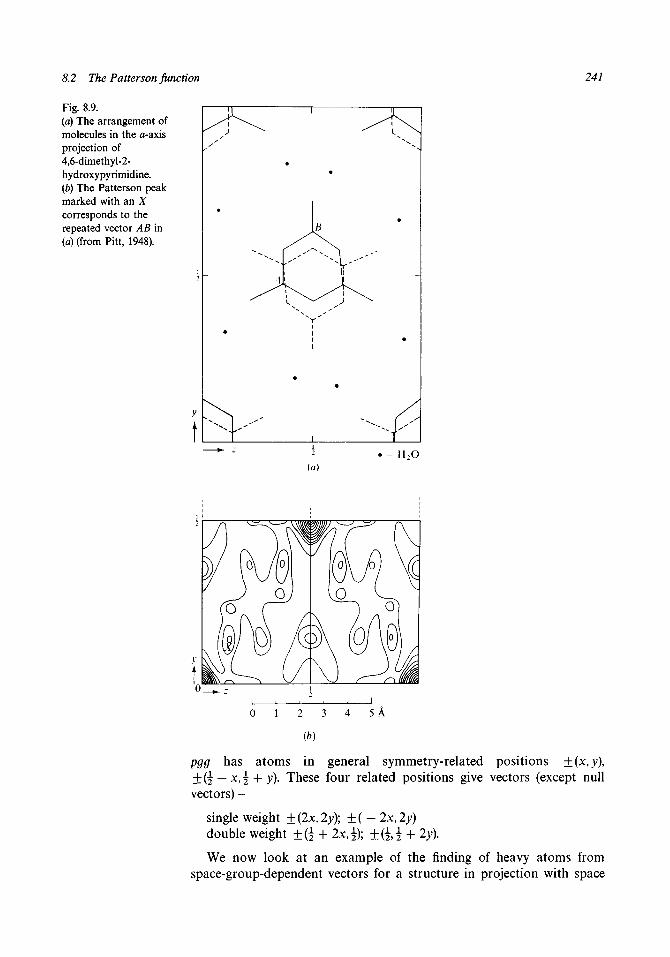
8.2 The Patterson function 241
Fig. 8.9.(a) The arrangement ofmolecules in the a-axisprojection of4,6-dimethyl-2-hydroxypyrimidine.{b) The Patterson peakmarked with an Xcorresponds to therepeated vector AB in(a) (from Pitt, 1948).
• = H2O(a)
(b)
pgg has atoms in general symmetry-related positions ±(x,y),±(i ~ x>i + y)- These four related positions give vectors (except nullvectors) -
single weight ±(2x,2y); ±( - 2x,2y)double weight ±(i + ±( i i + 2y).We now look at an example of the finding of heavy atoms from
space-group-dependent vectors for a structure in projection with space

242 The determination of crystal structures
Fig. 8.10.(a) The two-dimensionalspace group pmg(p2mg\(b) The artificialstructure C4H4N2C12.The mirror and glideplanes are indicated mand g, respectively.
group pmg (fig. 8.10(a)). The structure is an artificial one, (C2H2NC1)2,shown in fig. 8.10(fr), which we shall be using to illustrate various methods ofsolving structures. The molecule has a mirror plane which sits on thecrystallographic mirror plane m perpendicular to x. There is also a glideplane g perpendicular to y and these two symmetry elements generate atwofold axis - which gives a centre of symmetry in projection. The positionsof the atoms in one asymmetric unit of the unit cell are: Cx (0.175,0.083),C2 (0.125,0.333), N (0.175,0.583), Cl (0.100,0.833) and we also havea = 10 A and b = 6 A. The complete set of structure factors, calculated withthe program STRUCFAC for Cu Ka radiation (X = 1.542 A), are given intable 8.1 and the program FOUR2 uses the magnitudes to generate thePatterson map shown in fig. 8.11. [Chlorine contributions to the structurefactors are listed in table 8.2. These are discussed further in §8.3.]
Since chlorine (Z = 17) is much heavier than the other atoms the Cl—Clvectors should be clear in the Patterson map. For this space group thecoordinates of symmetry-related atoms are: (x, y); (\ — x, y); (x, y); (j + x, y)giving rise to single-weight vectors (2x, 2y\ (\ + 2x, 0) and the double-weightvector (2% 2y). The Patterson map has space group pmm and other vectorsare generated by the mirror planes. From knowledge of the structure, thedouble-weight vector is found at A, the highest non-origin peak in fig. 8.11,and the two single-weight vectors at positions B and C. The vector is not on
pmg No. 7
O©
©©
0
plmg
O
0
mm Rectangular
oOrigin at 2
(a)
(b)

8.2 The Patterson function 243
Fig. 8.11.The Patterson functionfor C4H4N2C12.
FACTOR CONVERTING TO DENSITY/UNIT AREAOUTPUT WITH Y HORIZONTAL AND ORIGIN
IS 1.5705TOP LEFT
0
0 100
9
10
11
12
13
14
15
16
17
18
21
22
23
24
25
26
29
30
31
5 8 ^ 3 7 ^ / 1 3 . 16 . 18 . 17 . 17 . 1 2 . 12 .
l o t " 12 . 14 . 1 3 . 2 1 . 30^; 2 2 . 9 . 1 2 .
11 14 . 12 . 8. 17 . 27 . 19 . 9 . 1 1 .
20
10
14
9
12
11
10
58 -"
14 14 17
10 11 12 13
0.1
10. 7. 9. 14 . 14 . 1 1 . 10 .
16 . 10 .
D12. 14. 20. 27.^ l^< 26,. 15
6. "2712. 15 . 2 1 . 3 0 / 37. 36 . 18.
™ 20. 2 3 . 26. 26"! ""23,* 19 . 2 1 .
. 2 3 . 15 . 12. 13 . 13 . 15 . 24.I
' 3 3 ^ 1 8 . 13 . 1 1 . 1 1 . 12. 15 . 18 .
15 . 10. 15 . 12. 7 . 9. 10 . 9.
1 1 . 12. 12. 7. 7. 10. 1 1 . 1 1 .
17. 19. 10. 9. 13 . 1 1 . 1 3 . 20.
18. 2 1 . 16. 15 . 14. 9. 14. 23 .
13 . 18 . 25 . 2 1 . 16. A^^3#6.>"(22.
12. 17. 31'.} 25. 20 . $6.
13 . 18. 25 . 2 1 . 16. 2 8 . ^ 3 6 . ^ 2 .
18 . 2 1 . 16. 15 . 14. 9. 14 . 23 .
17 . 19 . 10 . 9. 1 3 . 1 1 . 1 3 . 20.
25.XN34.
16. 15 .
1 1 . 8.
9. 1 1 .
1 1 . 16.
1 1 . 13 .
13 . 12.
25 . 26 .
3 0 / ^ 3 1 .\ ^
19. 18~.
10 . 1 1 .
1 1 . 1 1 .
17 . 10 .
19 . 14 .
15 . 1 8 .
1 1 . 17 .
1 5 . 1 8 .
19 . 14 .
1 7 . 10 .
z ^ -
2J5 < 1 2 .
16 . 12 .
1 1 . 1 1 .
9. 8.
1 1 . 10 .
1 1 . 1 5 .
1 3 . 1 8 .
2 5 . 2 1 .
30\ 24 .
' l 9 . 1 8 .
10 . 9 .
1 1 . 1 1 .
1 7 . 20 .
19 . 2 3 .
1 5 . 2 2 .
1 1 . 24 .
1 5 . 2 2 .
1 9 . 2 3 .
1 7 . 2 0 .
14 15 16
14 . 7 . iq 1 4
36.
17. 17 . 18 .
2 2 . 30-* 2 1 .
19 . 27 . 17.
1 1 . 14 . 14.
14. 1 1 . 1 3 .
30 . 21- 20 .
3^37:Vor
2 3 . " 26- r"26 .
1 3 . 1 3 . 12 .
12 . 1 1 . 1 1 .
9 . 7 . 12.
10 . 7 . 7 .
1 1 . 1 3 . 9.
9. 14 . 15 .
"28V. 16 . 2 1 .
0. 2 5 .
2 8 f 16 . 2 1 .
9. 14 . 15 .
1 1 . 1 3 . 9 .
16 . 1 3 .
1 3 . 14 .
8. 12.
9. 7.
1 1 . 8.
14. 12 .
2 1 . 15 .
2 3 . 20 .
15 . 2 3 .
1 3 . 18 .
15 . 10 .
10 . 19 .
16 . 2 1 .
2 5 . 18 .
31r» 17 .
25 . 18 .
16. 2 1 .
10. 19 .
12 . 10
14 . 11
10. 12
8. 9
1 3 . 14
12 . 10
20 . 20
3 6 / 44I
33\. 44\
15 . ^
1 1 . 11
17. 11
18. 12
13 . 14
12. 15
1 3 . 14
18 . 12
17 . 11
12. 12. 1 1 . 11
15 . 10 . 15 . 12. 7 . 9. 10 . 9. 10 . 1 1 . 10. 9.
33\ 18. 13 . 1 1 . 1 1 . 12. 15 . 18 . 19. 18 . 19. 18.
161 2 3 . 15 . 12. 1 3 . 13 . 1 5 . 24 . 3 0 / 3 1 . 30} 24.
2*0. 20. 23 . 26. 2 6 . ^ 2 3 . 19 . 2 1 . 25 . ?6T "25 . 2 1 .
12. 15 . 2 1 . 3 0 / 3 7 . 36. ^21. 18. 13 . 12. 13 . 18.
13 . 12. 14. 20. 2 7 > - 3 0 f ' 2 6 . 15 . 1 1 . 13 . 1 1 . 15.
8. 8. 1 1 . 13 . 1 1 . 14. 16 . 10. 1 1 . 16. 1 1 . 10.
10. 7. 9. 14. 14. 1 1 . 10 . 8. 9. 1 1 . 9. 8.
14. 12. 8. 17. 27. 19. 9. 1 1 . 1 1 . 8. 1 1 . 11 .
12. 14. 13 . 2 1 . 30/>.% 22 . 9 . 12 . 16. 15 . 16 . 12
. 16 . 18 . 17 . 17 . 1 2 . 12 . 25 . / 34~-25^ . 12.
I S I S 7 14 14 1? 77 47 77 >1 9
10 .
1 5 .
1 5 .
19 .
2 7 .
26 .
16 .
10 .
9 .
9.
1 2 .
9 . 7 . 12 . 15 . 10 .
12 . 1 1 . 1 1 . 1 3 . 18 .
1 3 . 1 3 . 12 . 1 5 . 2 3 .
2 3 . 2S. 26 . 2 3 . 20 .
36*. 37 . 30V 2 1 . 15 .
30S-27«?'2O. 14 . 12.
14 . 1 1 . 1 3 . 1 1 . 8.
1 1 . 14 . 14 . 9. 7.
19 . 27 . 17. 8. 12.
22 . 3 0M 2 1 . 1 3 . 14.
17 . 17 . 18 . 16 . 1 3 .
1 5 . 22
33<'*44
3 6V 44
20. !<f.
12 . 10
1 3 . 14
8. 9
10 . 12
14 . 11
12 . 10
the centre of peak B because of other vectors nearby. However, the specialpeaks along y = 0 and x = \ at A and C are sufficient to determine theposition of the chlorine atoms and peak B can then just be used asconfirmation.
The vectors at the special positions A and C in fig. 8.11 are space-group-dependent vectors and these generally occur when a symmetry elementinvolving a translation is present. For example, if the symmetry element 2X
is present along the b direction then atoms will be related in pairs withcoordinates (x,y,z) and (x,^ + y,z). The vector between such a pair ofatoms is (2x, \, 2z) and hence the section of the three-dimensional Pattersonmap y = \ should show all the vectors of this type. There may, of course, beother peaks in this section due to the accidental occurrence of vectors with acomponent y = \, but a high proportion of the peaks should be associatedwith the systematic peaks which show the structure projected down the b
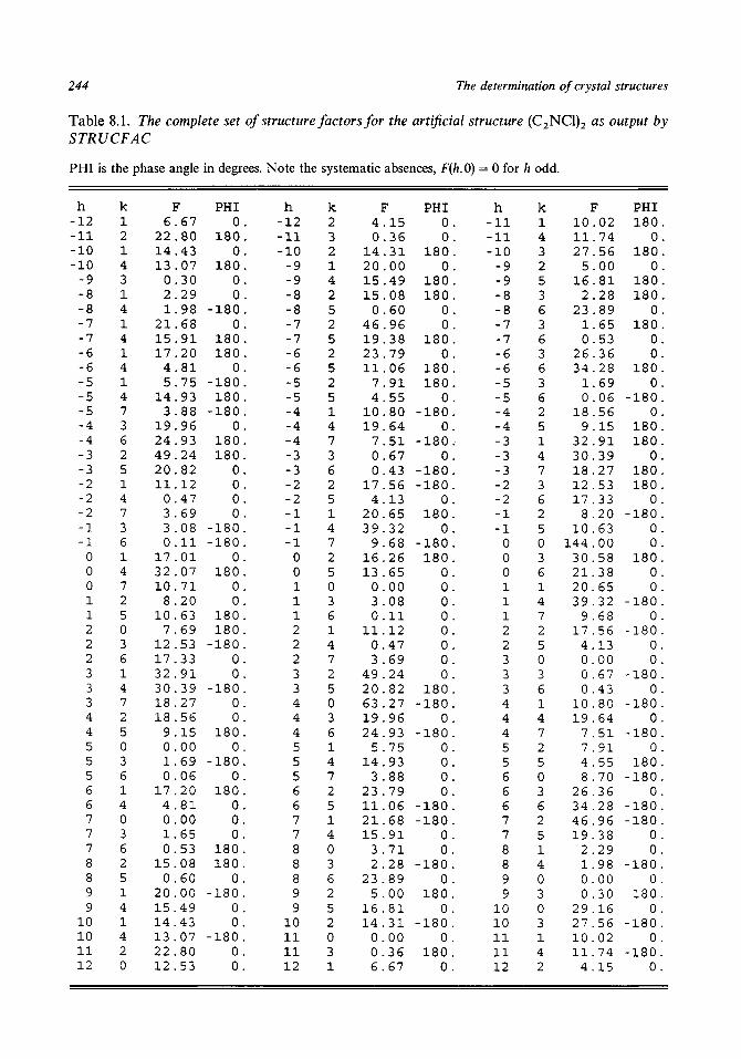
244 The determination of crystal structures
Table 8.1. The complete set of structure factors for the artificial structure (C2NC1)2 as output bySTRUCFAC
PHI is the phase angle in degrees. Note the systematic absences, F(h, 0) = 0 for h odd.
h- 1 2- 1 1- 1 0- 1 0
- 9- 8- 8- 7- 7-6-6- 5- 5- 5- 4- 4-3-3- 2- 2- 2- 1- 1
0001122233344555667778899
10101 112
k1214314141414736251473614725036147250361403625141420
F6 . 6 7
22.8014.4313.07
0.302 .291.98
21.6815.9117.20
4.815.75
14.933.88
19.9624.934 9 . 2 42 0 . 8 21 1 . 1 2
0 . 4 73.693.080.11
17.0132.0710.71
8.2010.63
7.6912.5317.3332.9130.3918.2718.56
9.150.001.690.06
17.204.810.001.650.53
15.080 . 6 0
20.0015.4914 .4313.0722.8012.53
PHI0 .
180.0 .
180.0 .0 .
-180.0 .
180.180.
0 .
-180.180.
-180.0 .
180.180.
0 .0 .0 .0 .
-180.-180.
0 .180.
0 .0 .
180.180.
-180.0 .0 .
-180.0 .0 .
180.0 .
-180.0 .
180.0 .0 .0 .
180.180.
0 .-180.
0 .0 .
-180.0 .0 .
h- 1 2- 1 1- 1 0
- 9- 9- 8- 8- 7- 7- 6- 6- 5- 5- 4- 4- 4- 3- 3- 2- 2- 1- 1- 1
0011122233444555667788899
1 01 11 112
k2321425252525147362514725036147250361472514036252031
F4.150.36
14.312 0 . 0 015.4915.08
0.6046.9619.3823.7911.06
7.914.55
10.8019.64
7.510.670.43
17.564 .13
20 .6539.32
9.6816.2613 .65
0.003.080 .11
11.120.473 . 6 9
49 . 2420 .8263 .2719.9624 .93
5.7514 .93
3.8823 .7911.0621.6815.91
3.712.28
2 3 . 8 95.00
16.8114 .31
0 . 0 00 . 3 66.67
PHI0 .0 .
180.0 .
180.180.
0 .0 .
180.0 .
180.180.
0 .-180.
0 .-180.
0 .-180.-180.
0 .180.
0 .-180.
180.0 .0 .0 .0 .0 .0 .0 .0 .
180.-180.
0 .-180.
0 .0 .0 .0 .
-180.-180.
0 .0 .
-180.0 .
180.0 .
-180.0 .
180.0 .
h- 1 1- 1 1- 1 0
- 9- 9- 8- 8- 7- 7- 6- 6- 5- 5- 4- 4- 3- 3- 3- 2- 2- 1- 1
0001112233344455666778899
1 01 01 11 11 2
k1432536363636251473625036147250361472503625140303142
F10.0211.7427.56
5.0016.81
2 . 2 82 3 . 8 9
1.650.53
26.3634.28
1.690.06
18.569.15
32 .9130.3918.2712.5317.33
8.2010.63
144.0030.5821.3820.6539.32
9.6817.56
4 .130 . 0 00.670.43
10.8019.64
7 .517 .914.558.70
26.3634.2846.9619.38
2 . 2 91.980.000.30
29.1627.5610.0211.74
4.15
PHI180.
0 .180.
0 .180.180.
0 .180.
0 .0 .
180.0 .
-180.0 .
180.180.
0 .180.180.
0 .-180.
0 .0 .
180.0 .0 .
-180.0 .
-180.0 .0 .
-180.0 .
-180.0 .
-180.0 .
180.-180.
0 .-180.-180.
0 .0 .
-180.0 .
180.0 .
-180.0 .
-180.0 .

8.2 The Patterson function
Table 8.2. Chlorine contributions to the structure factors o/(C2H2NCl)2
245
PHI is the phase angle in degrees. Comparison with table 8.1 shows that the indications of sign given bychlorine are mostly correct.
h-12-11-10-10-9-8-8-7-7-6-6-5-5-5-4-4-3-3-2-2-2-1-10001122233344555667778899
10101112
k1214314141414736251473614725036147250361403625141420
F4.07
13.8014 .4313.070.114.914.35
27.9624.4314.8712.150.000.000.00
29.3422.7337.1725.098.935.264.030.160.21
31.3317.4413.1326.4615.9318.9512.548.92
43.2627.8322.0116.8912.380.000.000.00
14.8712.150.000.190.314.824.26
15.3914.0814 .4313.0713.808.21
PHI0.
180.0.
180.-180.
0.-180.
0.180.180.
0.0.0.0.0.
180.180.
0.0.
180.0.0.
-180.0.
180.0.0.
180.0.
-180.0.0.
-180.0.0.
180.0.0.0.
180.0.0.0.
180.180.
0.-180.
0.0.
-180.0.0.
h-12-11-10-9-9-8-8-7-7-6-6-5-5-4-4-4-3-3-2-2-1-1-10011122233444555667788899
10111112
k2321425252525147362514725036147250361472514036252031
40
14151444
2622141100
1813100074
3117132616000854
3725382922000
14112724997
151314004
F.04.10.31.39.08.82.26.87.88.18.85.00.00.57.02.29.23.34.61.90.39.99.81.78.08.00.16.21.93.26.03.17.09.83.34.73.00.00.00.18.85.96.43.98.21.87.03.26.31.00.10.07
PHI-180.
0.180.
0.180.180.
0.0.
180.0.
-180.0.0.
-180.0.
-180.0.
-180.-180.
0.180.
0.-180.180.
0.0.
-180.0.0.
180.0.0.
-180.-180.
0.-180.
0.0.0.0.
-180.-180.
0.0.
-180.0.
-180.0.
-180.0.
180.0.
h-11-11-10-9-9-8-8-7-7-6-6-5-5-4-4-3-3-3-2-2-1-10001112233344455666778899
1010111112
k1432536363636251473625036147250361472503625140303142
F14 .0812.9927.5615.0313.269.217.870.190.31
26.3721.810.000.00
16.8912.3843.2627.8322.0112.548.92
26.4615.9368.0042.4929.1631.3917.9913.817.614.900.000.230.34
18.5713.0210.290.000.00
30.5526.3721.8126.8722.884.914.350.000.11
29.1627.5614.0812.994.04
PHI180.
0.180.
0.180.180.
0.180.
0.0.
180.0.0.0.
180.180.
0.180.180.
0.180.
0.0.
180.0.0.
-180.0.
-180.0.0.
-180.0.
-180.0.
-180.0.0.
-180.0.
-180.-180.
0.0.
-180.0.0.0.
-180.0.
-180.-180.

246 The determination of crystal structures
axis at double scale. A section of the Patterson function which showsspace-group-dependent vectors is called a Patterson-Harker section (Harker,1936). An example of a Patterson-Harker section is given in fig. 8.12; thiswas used to solve the structure of para-chlor-idoxy benzene (Archer, 1948).The X-ray measurements gave the space group as P2Ja with a = 14.4,b = 6.50, c = 8.11 A and p = 98.5° and four molecules of C1C6H4IO2 perunit cell. The symmetry gives related coordinates ±(x,y,z) and±( i + x>\ ~ y>z) a n d the vectors between related atoms, apart from nullvectors, are:
single weight ±(2x,2y,2z); ±(2x,-2y,2z)double weight +&£ + 2y,0); ±{\ + 2x,£,2z).
The two heavy peaks in fig. 8.12 are the iodine-iodine vectors correspondingto ± ( i + 2x,\,2z) and hence the iodine position may be derived.
It should be noted that the symmetry of the Patterson function need notbe the same as that of the structural group. The effects of space-groupsymmetry which lead to relationships between the phases of equivalentreflections, are lost in the Patterson function for which \F\2 is used as acoefficient. For all orthorhombic structures one has
hkl I2 = \F-m\2 = \Fh-kl\2 = \Fhkl\
2 = \Fm\2 = \2 = \Fhn\2 = \F-h-kl\2
and the Patterson function of all primitive orthorhombic space groups isPmmm. It can be shown (Buerger, 1950a) that for the 230 space groups thereare only 24 possible Patterson symmetries.
A very powerful technique for making use of Patterson maps is by the useof superposition methods. It was shown by Wrinch (1939) that if thecomplete set of vectors between atoms was available it would be possible torecover the original atomic positions. To see how this can be done there isshown in fig. 8.13(a) a set of five points and in (b) the vector set derived from
Fig. 8.12.The Patterson-Harkersection y = ^ forp-chlor-idoxy benzene(from Archer, 1948).
1 0 1 2 3 ALnlnJ 1 1 I 1 I 1

8.2 The Patterson function
Fig. 8.13.to Anon-centrosymmetric setof points.(b) The vector set.(c) Superposition on asingle-weight vector.For one vector set:
^ origin peak,« single peak,| double peak.For second set: #
(] origin peak,a single peak,Q double peak.
247
(a)
®
®
®
®
D I
(c)
these points. If two of the vector sets are now superimposed with a relativedisplacement equal to that of one of the single vectors then a number ofpoints exactly overlap. These are shown in (c) and they show the form of theoriginal set of points plus the centrosymmetrically related set connectedwith dashed lines. On the other hand, if the original unit is centrosymmetricas in fig. 8.14(a) giving the vector set (b) and if the overlap is made on asingle-weight peak then a single image of the set of points is produced.
It will be appreciated that this method depends on having available thevector set and this is not what one usually has from a Patterson function.The Patterson peaks are spread out and overlap, and errors in the observeddata can lead to random fluctuations which are as big as some of the smallerpeaks. Incidentally it should be noticed that if the displacement of twovector maps corresponds to a double-weight vector, as in fig. 8.14(d), thentwo images of the original set of points result. Similarly superposition withan rc-fold vector displacement gives n distinct images.
If the relative positions of more than two points of the original set are

248
Fig. 8.14.(a) A centrosymmetricset of points.(b) The vector set.(c) Superposition on asingle-weight vector.(d) Superposition on adouble-weight vector(symbols as in fig. 8.13).
The determination of crystal structures
(b)
(c)
id)
known then the image of the set of points can be recovered by multiplesuperposition. This type of procedure is very necessary when one is using areal Patterson function; firstly, it is usually difficult to find a single-weightpeak and, secondly, there will always be a number of chance peaks whichwill confuse the image obtained from the overlap function. There are

8.3 The heavy-atom method 249
various functions of the overlapped Patterson maps which can be taken. Ifthe displacement of the two map origins is R then one can find the productfunction P(r)P(r + R) or the sum function P(r) + P(r + R). A functionproposed by Buerger (1950b) is the minimum function, M{P(r), P(r + R)},which means the least of the two quantities P(r) and P(r + R). If r and r + Rcorrespond to the positions of peaks of interest then each of the peaksshould at least have a single weight but might be heavier because of theaccidental overlapping of peaks. By taking the minimum function onereduces the amount of spurious information in the result. When the relativepositions of a number of atoms are known the use of the minimum functioncan lead to the solution of quite complicated crystal structures.
The quality of Patterson functions can be improved by various sharpeningprocedures. Ideally one would like the Patterson map corresponding topoint atoms but if one tries to achieve this by using \U\2 instead of | F |2 thenthe termination of the Fourier series leads to considerable diffraction ripplearound the peaks. The negative regions thus introduced may reduce oreliminate other peaks. However to take the observed \F\2 will probablylead to very diffuse peaks giving considerable peak overlap. In fact if onemodifies the |JF|2 'S by any smooth function of s ( = 2sin0/,l) then theindividual peaks retain their spherical symmetry. A 'rule-of-thumb' whichgives reasonable results is so to modify the \F\2 that the average value of themodified | F \2 for the region near the edge of the sphere of reflection is about0.1 times the average of | F |2 near the centre of the sphere. The modificationcan be made with an analytical expression, such as exp(Ks2), or by ahand-drawn function on graph paper - it is not a very critical operation.With judicious sharpening one can pick out useful vectors which wouldotherwise be lost. Oversharpening, on the other hand, leads to theappearance of greater resolution but the extra peaks can be of diffraction-rippleorigin and some of them can be quite spurious.
8.3 The heavy-atom method
When a structure contains a large number of light atoms and a few heavyatoms the structure can frequently be solved in a straightforward way. Letus consider a centrosymmetric structure containing in each unit cell n heavyatoms whose positions can be located through the use of the Pattersonfunction. If the contribution of the heavy atoms to the structure factor ofindex h is Ch then we have
N-nFh = ch + Z /)cos(27ihT</) = Ch + Kh, say, (8.8)
where N is the total number of atoms in the unit cell. Sometimes thecontribution of the heavy atoms can dominate to the extent that most of theF s will have the same signs as the C's. Either a Fourier synthesis can becalculated with the signs of the C's completely accepted or discretion can beexercised and the sign only accepted if the magnitude of C is sufficiently high.
A standard technique of solving a stereochemical problem is to prepare aheavy-atom derivative of the substance in question. In selecting the heavy

250 The determination of crystal structures
atom a careful balance has to be struck. If the heavy atom is too light it willbe a poor determiner of signs and the structure will not be soluble. On theother hand, the contribution of too heavy an atom will so dominate theintensities that the errors in intensity measurement may become comparableto the contribution of the lighter atoms. A rule-of-thumb which works wellif there are a number nL of almost-equal light atoms and a number nH ofheavy atoms is to have
I/2 = I/2 (8-9)heavy atoms light atoms
which, from equations (7.29) and (7.32), indicates that the average contributionsof the light atoms and heavy atoms to an intensity should be equal.
The principle of the heavy-atom method can be illustrated with thesynthetic structure (C2H2NC1)2 shown earlier in fig. 8.10(b). The position ofthe chlorine atom could be determined from the Patterson function (fig.8.11) and the chlorine atom forms a substantial part of the total scatteringpower. The left- and right-hand sides of equation (8.9), ignoring thehydrogen atoms, are 289 and 121, respectively. The program STRUCFACwas used to calculate structure factors from the chlorine positions aloneand these are shown in table 8.2 (p. 245). Of the 156 structure factors thereare 14 for which the chlorine contribution is zero (excluding 6 structurefactors which are systematically zero) so that no sign indication is given. Ofthe remaining 136 structure factors all but 8 have their signs indicatedcorrectly by the chlorine contribution and 4 of these 8 have very smallstructure amplitudes. The program HEAVY listed in appendix VI, enablesthe output file from STRUCFAC to be modified and this has been used tomake the structure amplitudes zero for the 20 reflections for which there areno sign indications and to change the signs (phases) of the 8 incorrectlyindicated by the chlorine contribution. The modified data file was theninput to FOUR2 to give fig. 8.15, a Fourier map which shows clearly thepositions of the light atoms.
In this example all the signs of the structure factors were taken as those ofthe chlorine contributions but, in fact, it is possible to determine theprobability that the sign of the structure factor is correctly given by theheavy-atom contribution. From equation (8.8) it can be deduced that if Fh
and Ch have the same sign then
l K k l = l l ^ h l - i q j l (8.10a)
whereas if Fh and Ch have opposite signs then
\Kh\ = \Fh\ + \Ch\. (8.10b)
From equation (7.22) it can be seen that, from structure-factor statisticsalone and not taking account of any other information, the probabilitydistribution of Kh is given by
P(K) = (27il')"iexp( - K2/2I') (8.11)

8.3 The heavy-atom method 251
Fig. 8.15.Fourier map forC4H4N2C12 with signsgiven by the chlorineatoms. The light atomsare in the positionsoutlined by a singlecontour.
FACTOR CONVERTING TO DENSITY/UNIT AREA IS 0.1955OUTPUT WITH Y HORIZONTAL AND ORIGIN TOP LEFT
10 11 12 13 14 15 16 17 18 19 20
3
9
7
9
11
- 3
- 2
8
- 2
- 3
11
9
7
9
3
- 9
3
9
7
9
11
- 3
- 2
8
- 2
- 3
1 1
9
7
9
3
- 1
- 2
5
4
- 2
12
19
9
4
9
19
12
- 2
4
5
- 2
1
6
- 2
- 7
- 2
6
2
- 4
- 3
- 4
2
6
- 2
- 7
- 2
6
4 .
4 .
. 3 .
. - 3 .
3
3
8
5
. 1 7 . 10
/ 2 ; > l S
. -3 .
. 9.
,J7~
. - 3 .
. 3 .
4 .
. 4 .
. 13 .
0 .
. - 2 .
. 9.
. 2 .
. -12 .
. 2 .
. 9.
. - 2 .
. 15 v
. 2{.\
. 0.. -4 .
i n
7
1
V
5
8
3
3
12
-6
-4
-1
4
- 1 0
4
-1
-4
- 6
9
. - 1 .
. 0.
. 2 .
. -4 .
. 1.
. - 4 .
• " 2 .
. 8.
. - 2 .
. -4 .
. -4 .
. 2 .
. 0.
. - 1 .
. 7.
. - 2 .
. 6.
. - 5 .
. 6.
. 1.
. -4 .
. - 2 .
7
1 .
4 .
5 .
0 .
6.
6.
- 2 .
- 3 .
- 2 .
6 .
0 .
5 .
4 .
1 .
9 .
1.
9 .
3 .
- 3 .
3 .
9.
2 .
V?'
1 .
. 7.
3 .
2 .
14 .
1 8 .
7 .
- 1 .
0.
4 .
0 .
- 1 .
7.
18.
14 .
2 .
3 .
5 .
1.
2 .0.
2.
1.
- 4 .
1 .
- 4 .
1 .
11 .
2 .
0 .
2 .
1 .
5 .
0 .
1 5 .
(25 .
8."*
- 5 .
1 .
7 .
1 .
- 5 .
2'5~
x5^«
0 .
5 .
- 3 .
-4 .7 .
10.
8.
5 .
0 .
5 .
0 .
5.
14.
8 .
1 0 .
7 .
- 4 .
7
5 .
2 .
5 .
1 3 .
s
12 .
7 .
0.- 6 .
0 .
7 .
12.
- 5 .
2 .
5 .
- 3 .
1.
3 .- 4 .
- 2 .
1 0 .
- 2 .
1 0 .
- 3 .
- 2 .
0 .
2 .
3 .
4 .
0.
- 3 .
0 .
4 .
3 .
2 .
0 .
- 2 .
- 3 .
-4 .
9 .
6.0.
4 .
23 i
9 .
- 3 .
9 .
t *19s.-^XP/.
-2.
- 4 .
3 .
1 .
4 .
0 .
6 .
9 .
1 .
1 .
2 .
5 .
7 .
3 .
1 .
3 .
4 .
3 .
1 .
3 .
7 .
5 .
2 .
1 .
- 7 .
2 .
5 .
7 .
1 .
3 .
4 .
3 .
1 .
3 .
7 .
5 .
2 .
1 .
Q .
9 .
6 .
0 .
4 .
17.
9.
- 3 .
9 .
2 3 /
4 .
0 .
6 .
9 .
-4 .
- 2 .
0.
2 .
4 .
0 .
- 3 .
0 .
4 .
3 .
2 .
0 .
- 2 .
- 3 .
1
1
3
- 4
- 2
. -4
7
. 10
. 8
,19 . 14
27.S; 5
To. 0
- 2
10
-27-
A2-2
- 4
3
1
- 3
2
5
13
7
0
- 6
0
7
12
13
5
2
5
?
. 5
. 0
*\ 5/
. 8
. 10
7
- 4
- 3
0
15/"*125
V.
- 5
1
7
. 1
. -5
. 8
.,'25
As. 0
. 5
?
1 .
. 2 .
0 .
. 2 .
. 11 .
1.
. -4 .
. 1.
. -4 .
1 .
. 2 .
. 0.
2 .
. 1.
. 5.
. 2.
"" \
. - 1 .
. 0.
4 .
. 0.
. - 1 .
7 .
" l 8 .
.-f4.
. 2 .
. 3 .
1 .
- 1 .
7 .
2 .
2 .
9 .
3 .
- 3 .
3 .
9 .
2 .
7 .
- 1 .
1 .
9 .
4 .
5.
0.
6.
6.
- 2 .
-3 .
- 2 .
6.
6.
0 .
5 .
4 .
1 .
7
- 2
26
lift'
1 .
6 .
- 5 .
6 .
1 .
2 6 ^
- 2 .
7 .
0 .
2 .
- 4 .
1.
-4 .
- 2 .
8 .
- 2 .
-4 .
1.
- 4 .
2
0 .
-1 .
7 .
- 6
- 1 .
4 .
-10 .
4 .
- 1 .
^2}
- 6 .
1 2 .
3 .
8.
5.
10.
5.
1 .
7 .
1 .
5.
10.
5 .
8 .
3 .
3 .
9
- 4
A" -2.
9.
2.
- 1 2 .
2 .
9 .
J2/7)
- 4 .
13 .
4 .
3 .
- 3 .
1 7 .
2*7.
- 3 .
9 .
27 .
1 7 -
- 3 .
3 .
4 .
4 .
i n
6
-2.
V7-' - 2 .
6.
2.
-4 .
- 3 .
-4 .
2 .
6 .
t
- 2 .
6 .
1.
- 2 .5.
4 .
- 2 .
12.
/
4 .
9 .
- 2 .
4 .
5 .
- 2 .
g
7
q
11
-2
8
- 2
- 3
11
97
9
3
- 9
3
97
9
11
-3- 2
8
- 2
-3
1 1
9
7
9
3
-1 .
13
14
15
16
17
18
19
20
21
22
23
24
25
26
27
28
29
30
31
32
where Z' = £ /? . The probability that Fh and Ch have the same sign, P+,j= 1
will be related to the probability that they will have opposite signs, P_, by
P+_exp{-( |Fh[- |CJ)2 /2E'}T) ( / I T7 I 1 I /"> I \ 2 / ^ W V V * /
The expression (8.12) uses the distribution (8.11) to determine the relativeprobability of having the two values of | X h | given by equation (8.10).Expression (8.12) can be simplified to
(8.13)

252 The determination of crystal structures
and if we use the relationship
P + + P_ = 1 (8.14)
then we obtain
P+=Hitanh(|Fh||Ch|/r). (8.15)
Woolfson (1956) showed that a Fourier synthesis can be calculated withweighted Fs which gives the greatest signal-to-noise ratio in showing thelight atom. The Fourier coefficients used for the synthesis are
| F h | x ( 2 P + - l ) x ( s i g n o f C h ) .
The synthesis with modified coefficients gives a clearer density map thanis obtained by accepting all signs from the heavy-atom contribution or anyarbitrary scheme of accepting or not accepting the heavy-atom sign. For theexample we have used here the advantage would be hard to detect becauseperfect data are being used and the heavy-atom contribution is relativelylarge. However if there was one chlorine atom in the presence of, say, 30carbon atoms then the left- and right-hand sides of equation (8.9) would be289 and 1080, respectively. The contribution of chlorine would be much lessreliable in this case and a map with properly weighted coefficients would bemuch easier to interpret.
Sometimes the first map obtained by the heavy-atom method does notgive all the light atoms but rather a fragment of the remainder of thestructure. In this case the atoms which are clearly indicated in the map canbe added to the heavy atoms and the new combination of atoms in knownpositions will give more reliable sign indications. A new map may thenreveal further atoms and the process can be repeated until the structure iscompletely determined. There are cases where, for a light-atom structuresome fragment of the structure can be found, for example by matchingvectors from some symmetric part of a structure with the peaks of aPatterson map. The heavy-atom method can then be used to try to find theremainder of the structure - although the term 'heavy atom' applied to themethod is somewhat inappropriate in such a situation.
The heavy-atom method can also be of value for solving non-centrosym-metric structures. However if there is only one heavy atom then this may bearbitrarily placed at the origin and all the phases are indicated as zero. Thiswill give rise to a Fourier synthesis which has a false centre of symmetry andit may be difficult to pick out the peaks corresponding to the structure. Ifthere are two equal heavy atoms then the situation is similar since the centreof the pair may be taken as origin and all the phases will be 0 or it.
When there is a non-centrosymmetric heavy-atom group which can belocated by Patterson methods then the phase from this group can be used asa first phase for a Fourier synthesis. Sim (1957, 1959, 1960) has made astatistical analysis of the errors in the phase angles obtained from the heavyatoms alone and has also found the weighting scheme for structureamplitudes which gives the best Fourier synthesis - in the sense of havingthe highest signal-to-noise ratio. The map calculated is

8.3 The heavy-atom method 253
p'(r) = £ W(h)F(h)cos{27ihT - #1)}.h
(8.16)
The weight imposed on the structure amplitude is
W(h) = I1(X)/I0(X) (8.17)
where 7X and / 0 are modified Bessel functions and X = 2 | F(h) 11 C(h) | /E'.The form of I^Xyi^X) as a function of X is shown in fig. 8.16.
Fig. 8.16. I\(X)The Sim weighting I0(X)curve. i Q _
Fig. 8.17.The synthetic structureC3H5N2ONa2.
0.5 -
An illustration of the use of Sim weighting is given by application to thesynthetic structure C3H5N2ONa2, space group pg with a = 8 A, b = 6 A,illustrated in fig. 8.17. The coordinates of atoms in one asymmetric unit are:Na (0.937,0.250), Na (0.437,0.583), 0(0.063,0.667), N (0.156,0.417),N (0.219,0.958), C (0.125,0.167), C (0.375,0.125), C (0.344,0.375).

254 The determination of crystal structures
Fig. 8.18.Fourier map forC3H5N2ONa2 withphases from the sodiumatoms and Sim weights.
The sodium atoms are regarded as 'heavy' and the left- and right-hand sidesof equation (8.9) are, excluding hydrogen, 242 and 270, respectively. In thiscase the heavy atoms are not so dominant as in the previous syntheticstructure (C2H2NC1)2, and tables 8.3 and 8.4 show the structure factors forCu Ka radiation (X = 1.542 A) for the complete structure and the contributionsof the sodium atoms, respectively. It will be seen that the sodium atoms tendto give reasonable phase estimates, mostly within 60° or so, but with somenotable exceptions. The program HEAVY was used to produce an input filefor FOUR2 which had Sim-weighted Fourier amplitudes and the phasesfrom the sodium contributions. The resultant map is shown in fig. 8.18; thesodium atoms appear clearly, because they have been the source of thephases, but the other atoms appear less clearly and some spurious densitycan also be seen. However with stereochemical knowledge of the moleculethe map can be interpreted to lead to a complete solution of the structure.
If only a fragment of the non-heavy-atom structure can be found from aSim-weighted map then the iterative procedure described for centrosymmetricstructures can be used. The use of Sim-weighted Fourier syntheses is animportant procedure in X-ray crystallography for going from a knowledgeof a partial structure to a complete structure determination.
FACTOR CONVERTING TO DENSITY/UNIT AREA IS 0.1231OUTPUT WITH Y HORIZONTAL AND ORIGIN TOP LEFT
10 11 12 13 14 15 16 17 18 19 20
0
1
2
3
4
5
6
7
8
9
10
1 1
12
13
14
15
16
17
18
19
20
2 1
22
23
24
3
-2
0
15
23
20
12
1
14
10
5
7
- 1 9
i s '
1V3
- 5
10
6
8
13
5
2
7
11
3
5 .
4 .
/
l l )
5 .
" 16.
1 2 .
*8 .^
2 .
5 . ,
~dr(\ 7 5 \N S ^
9 ^
4 .
8 .
9 .
1 2 .
7 .
3 .
6 .
8 .
4
- 3
4
2
4
17
7
16
19
v l l
1
2 1 '
5?92
- 1
8
4
- 1
3
7
10
8
. 6
. 4
. 12V
. 3
. 12
. 2
. 16
• # '
. 12""" —
7
? - 8
H. -7
. 4
. 3
. -3
. -6
. -5
f"l4
\ l 9
. 6
X". 17
. 3~
. 14
. 4
. 5
.^ -3
. J' - i
. -4
. -4
. 3
. 6
. -5
' ^
0 .
1 6 .
1 6 .
" T.1 6 .
3 .
1 .
4 .
- 1 .
5 .
- 1 .
v 8 .
/' 9 .
8 .
6 .
4 . ,1
6. ^
8 .
0 .
,.15*»
VIOO.
5 .
8 .
1 5 .
"~2*".
5 .
1 .
^ 9 .
1 4 .
3 .
10/15.
1 0 J
1 3 7
1 4 .
4 .
3 .
-4 .
8 .
5 .
0 .
6 .
,14.
8 .
6 .
Na
2 3 .
2 4 .
1 3 .
- 2 .
- 2 .
- 2 .
0
- 4
18
) l 2
19
16
0 .
5 .
0 .
1 1 ? t 5 .
8 .
6 .
6 .
1 1 .
5 .
1 1 /
- 5 .
* 1 .
3 .
1 5 , .
1 6 .
1 3 .
7 .
— —4 .
- 1 .
4 .
8 .
7 .
11 .
7 .
"1 N 2.
* 1 3 . Is-12./ 13.
/ 9 .
{ 4 .
C l \
0 .
- 3 .
3 .
- 1 3 .
1.
- 4 .
" l o . .
1 7 .
\19."
•20.
9 ^
- 2 .
2 .
8 .
6 .
"VI.
- 5 .
13 '' '(
\
-19 r
7 .
5 .
• . V
1 4 .
1 .
'f2T2 0 .
2 3 .
<
0 .
- 2 .
8 .
6 .
3 .
7 .
1 2 .
9 .
8 .
4 .
9 V
* "5.-
2 .
8 .
1 2 .
1 6 .
57"
6 .
\ 7 .\
34 .
5 .
8
10
7
3
- 1
4
8 .
- 1 .
1 .
l l T
1 9 .
1 6 .
"-77
1 7 .
4 .
2 .
4 .
- 3 .
4 .
' 14 >
V-1T- 6 .
- 3 .
3 .
4 .
-7 .
N - 5 .
Na ;V )
7 .
- 1 2 .«s
2 4 .
1 6 .
— 2T
12 .
3 .
1Z."/(16.V
4 ^
6 .
\M>- 5 .
6 .
3 .
- 4 .
- 4 .
- 1 .
O.0
V,12 . i
5 .
- 1 .\
j9'.
4 .
14 .
3 .
— ~"
2 4 .
14 .
6 .
^ 9 7 _
0 .
8 .
6 .
4 .
6 .
8 .
9 .
8 .
- 1 .
5 .
- 1 .
4 .
1 .
3 .
1 6 .
8
1 6 .
1 6 .
9-7
0 .
6 .
8 .
< 1 4 .
0 .
5 .
8 .
- 4 .
3 .
4 .
101i
1 0 ^
2 .
1 5 .
1 1 .
""* 6L
5 .
^ 7
h/-5
. 4 .
. - 1 .
. 4 .
V N
5
^ £1 1
'7
6
8
1 1V
- 2
- 2 .
- 2 .
2 4 .
2 3 .
1 5 .
1 4 .
-*>
1 .
5 .
. 7.
.^i-3-r
1 3 .
^ 1 6 .
3 .
) 5.
0 . -
5 .
0 .
1 7 .
1 6 /
1 9 . \
; 1 2 -
1 8 .
-4 .
0 .
2
- 2
9
-r-i 2 1
19
9
17
1 0 .
- 4
1
13
3
- 3
0
4 .
k 9.
1 2 ,
1 3 .
1 3 .
7 .
8 .
_2
' > &
N 3
x20. 12
• l ^
. 14"
5
7
- 1 9
1 8 '
{3
- 5
^ 0
6
8
13
\ 5
/ 2
7
1 1

8.4 Isomorphous replacement 255
8.4 Isomorphous replacement
Very often it is possible to have chemically similar materials in which one ormore atoms or groups in one compound are replaced by one or moresimilar atoms or groups in the other. Sometimes the substitution can befairly straightforward - one halogen atom for another or one alkali metalfor another - but can be less simple. For example, in fig. 8.19 there areshown the molecular forms of 2-amino-4-methyl-6-chloropyrimidine and 2-amino-4,6-dichloropyrimidine (Clews & Cochran, 1948) which differ in thatthe methyl group of the first is replaced by a chlorine atom in the second.
The crystals of the two materials look rather similar (long needles) andboth have four molecules in a monoclinic unit cell of space group P2Ja.The cell dimensions of the two structures are:
P
methylchloro
16.43 A16.45 A
4.00 A3.85 A
10.31 A10.28 A
109°108°
An examination of the X-ray data reveals that the diffraction patterns arestrikingly similar in appearance and it is clear that, in terms of crystalstructure, the atoms must be similarly arranged except that in one case amethyl group is replaced by chlorine.
Two crystal structures bearing this sort of relationship to each other aretermed isomorphous and from the differences in their diffraction patterns itis often possible to obtain a complete structure determination.
Let us take the case where we have two isomorphous structures whichdiffer in having n atoms of type A in one replaced by atoms of type B in theother. Then the structure factors of vector index h for the two compoundscan be written as
Fig. 8.19.The molecular forms ofthe isomorphouscompounds2-amino-4-methyl-6-chloropyrimidine and2-amino-4,6-dichloropyrimidine.
H
H—NL
2-amino-4-methyl-6-chloropyrimidine
H
H—N.
L 2-amino-4,6-dichloropyrimidine

256 The determination of prystal structures
Table 8.3. Structure factors for the synthetic non-centrosymmetric structure C3H5N2ONa2
PHI is the phase angle in degrees.
h- 1 0
- 9- 8- 7- 7- 6- 6- 5- 5- 4- 4- 3- 3- 3-2-2- 1- 1
00011122333444556677889
10
k122142525251473625036147250361472514030310
F4.53
11.836.65
14.0211.4117.8210.2114.61
5.766.12
11.5130.08
3.4910.9518.01
7.3628.7215.37
124.000.00
13.574.93
28.275.24
32.243.032.978.194.15
14.7611.9510.3314.61
5.7614.15
8.238.716.84
14.955.96
12.0816.02
PHI1 .1 .
-46.126.135.-69.115.
0 .179.-45 .
9 3 .132.
7 5 .- 4 1 .-10.161.
-167.-147.
0 .0 .
-164.-130.
-53 .4 9 .
125.-134.-180.-169.
4 5 .1 9 .1 6 .
-100.0 .
- 1 .4 8 .
-149.-180.
110.-180.-125.
168.180.
h- 1 0
- 9- 8- 7- 7- 6- 6- 5- 5- 4- 4- 3- 3- 2- 2- 2- 1- 1
00011222333445556677889
10
k233253636362514736147250361472503625141421
F3.036.695.96
13.384.62
15.135.30
14.637.16
26.371.71
15.8711.0516.01
9.634.578.974.500.00
12.510.00
28.7215.3717.2318.01
7.3630.08
3.4910.95
6.1211.51
2.2814.63
7.1617.8210.2114.0211.41
4.868.10
11.834.53
PHI-20.
4 1 .5 5 .2 2 .
-73 .-34.
4 8 .-140.-128.
-14.-108.
174.-153.-159.
7 7 .2 4 .
-35 .- 4 .
0 .-132.
0 .-167.
3 3 .0 .
170.161.-48.
7 5 .139.-45 .-87.
0 .4 0 .
-128.-69.-65 .-54.135.-99.
-139.1 .
-179.
h- 9- 8- 8- 7- 6- 6- 5- 5- 4- 4- 4- 3- 3- 2- 2- 1- 1- 1
00111222334445566677899
10
k114314141473625147250361472503614036252032
F12.08
4.868.106.84
14.158.23
36.835.30
14.7611.9510.33
8.194.15
32.243.034.93
28.275.24
19.660.00
17.828.974.50
16.019.634.57
15.8711.0516.6826.37
1.7136.83
5.3014.9815.13
5.3013.38
4.626.650.596.693.03
PHI-12.
8 1 .-139.
-70.-132.-149.
170.138.
-161.1 6 .8 0 .1 1 .4 5 .
125.4 6 .5 0 .
-53 .-131.
105.0 .0 .
145.-4 .2 1 .7 7 .
-156.174.
2 7 .-180.
166.-108.
-10.138.180.146.
4 8 .2 2 .
107.-46.
-180.-139.
-20.

8.4 Isomorphous replacement
Table 8.4. Contributions to the structure factors of the Na atoms of the syntheticnon-centrosymmetric structure C3H5N2ONa2
PHI is the phase angle in degrees.
257
h- 1 0
- 9- 8- 7- 7- 6- 6- 5- 5- 4- 4- 3- 3- 3- 2- 2- 1- 1
00011122333444556677889
1 0
k122142525251473625036147250361472514030310
F4 . 6 4
1 1 . 0 98.016 . 1 5
1 2 . 2 77 . 6 65 . 1 18.43
1 3 . 0 10 . 1 78 . 8 0
2 6 . 5 47 . 3 9
1 0 . 5 72 0 . 4 61 1 . 6 22 7 . 7 4
6.964 4 . 0 0
0 . 0 01 7 . 1 61 2 . 9 52 0 . 1 8
4 . 6 61 1 . 5 1
7 . 0 90 . 0 00 . 0 80 . 0 4
14 . 8 70 . 1 36.388 . 4 3
1 3 . 0 17 . 9 16 . 2 00 . 0 00 . 0 2
1 7 . 1 50 . 3 75 . 1 68 . 8 1
PHI6 0 .3 0 .
-60.150.150.-60.120.
3 0 .-150.
-60.120.150.-30.-30.
0 .180.
-150.-150.
0 .0 .
180.-30.-30.150.120.-60 .
0 .-90 .-90 .
6 0 .-120.-120.
3 0 .3 0 .6 0 .
-120.0 .
-90.-180.
0 .150.180.
h- 1 0
- 9- 8- 7- 7- 6- 6- 5- 5- 4- 4- 3- 3- 2- 2- 2- 1- 1
00011222333445556677889
1 0
k233253636362514736147250361472503625141421
F4.190 . 0 20 . 3 7
1 5 . 0 04 . 2 4
1 3 . 4 39 . 2 70.060 .03
2 4 . 5 00 . 1 99 . 8 7
1 5 . 3 71 2 . 9 3
8.624 . 9 40.040.100 .00
1 2 . 9 20 . 0 0
2 7 . 7 46 . 9 6
2 6 . 4 82 0 . 4 61 1 . 6 22 6 . 5 4
7 . 3 91 0 . 5 7
0 . 1 78.800 .000 .060 .037 . 6 65 . 1 16 . 1 5
1 2 . 2 70 . 2 16.83
11.094.64
PHI-60.-90.180.
3 0 .-150.
0 .0 .
9 0 .9 0 .
0 .0 .
-150.-150.-120.
6 0 .6 0 .9 0 .
-90 .0 .
6 0 .0 .
-150.3 0 .
0 .180.180.-30.-30.150.-60.-60.
0 .-90 .
9 0 .-60.-60.-30.150.
-120.-120.
3 0 .- 1 2 0 .
h- 9- 8- 8- 7- 6- 6- 5- 5- 4- 4- 4- 3- 3- 2- 2- 1- 1- 1
00111222334445566677899
1 0
k114314141473625147250361472503614036252032
F5 . 1 60 . 2 16.830.027 . 9 16 . 2 0
2 0 . 8 36 .55
1 4 . 8 70 . 1 36 . 3 80 .080 . 0 4
1 1 . 5 17.09
12.9520.18
4 . 6 61 7 . 6 0
0 . 0 00 . 0 00 . 0 40 . 1 0
1 2 . 9 38.624 . 9 49 . 8 7
1 5 . 3 70 .38
2 4 . 5 00 .19
2 0 . 8 36 .55
1 6 . 7 81 3 . 4 3
9 . 2 71 5 . 0 0
4 . 2 48 . 0 10 .000.024.19
PHI-30.
6 0 .-120.
9 0 .-120.-120.
150.150.
-120.-120.
6 0 .9 0 .
-90.120.120.150.-30.-30.120.
0 .0 .
-90.-90.
6 0 .6 0 .
-120.-150.
3 0 .-180.
180.0 .
-30.150.180.180.
0 .3 0 .3 0 .
-60.0 .
9 0 .-60.

258 The determination of crystal structures
(h)A = Kh +fA t exp(27iih-r7.)7 = 1
and
(FJB = Kh +fB £ exp(27iihT,.), (8.18)
where Kh is the contribution of the atoms common to both structures andthe summation is over the positions of isomorphously-exchangeable atoms.If this summation is written as Ch we have
(Fh)A = Kh +fACh
and
(Ft)B = Kh+fBCh. (8.19)
For centrosymmetric structures these equations can lead directly tophase information. The values offA,fB, \ (Fh)A | and | (Fh)B | will be known; ifthe value of Ch is known as, for example, when the isomorphously-replaceableatoms are in special positions, then the signs of the F s may be found.
Let us consider
| (Fh)A | = 92, | (Fh)B | = 7 8 , / , = 12 , / , = 20, Ch=-2.
The only reasonable solution of equations (8.19), allowing for some errorsof measurement, is
(Fh)A = + 92, (Fh)B = + 78, Kh = + 117.
The signs of (Fh)A and (Fh)B will both be established as positive in thisexample. Another set of values might be
\(Fh)A\ = 8, \(Fh)B\ = 10 , / , = 12 , / , = 20, Ch = - 2.
Since, from equations (8.15), we have
(8.20)
and the value of the right-hand side is +16, the only reasonable values forthe structure factors are (Fh)A = + 8 and (Fh)B = — 10.
The situation where the F's have opposite signs is quite rare if theisomorphously-replaced (abbreviated to i-r) atoms are not too powerfulscatterers. It is possible with careful measurements to record structurefactors with sufficient accuracy to measure the changes of scattering due toreplacements of Na by K (ZB -ZA = 8), Cl by Br (ZB - ZA = 18) or O by S(ZB — ZA = 8). Clearly it is important that the two sets of data should bereasonably well scaled together.
Let us now consider the situation for a centrosymmetric structure whenwe do not know the sign or magnitude of Ch. From equation (8.20) it can beseen that (Fh)A — (Fh)B ( = ^h) is the structure factor for scatterers ofscattering factors/, — fB at the positions of the i-r atoms. If we accept thatonly rarely will a sign change occur then we know the magnitude of \jjh butnot its sign. However a Fourier synthesis with \jj^ as coefficients will give aPatterson map of the difference of the two structures which should show

8.4 Isomorphous replacement 259
peaks only at positions corresponding to vectors between the i-r atoms. Ifthis simple Patterson map can be interpreted then the positions of the i-ratoms will be found and the signs of the structure factors can be determined.
This process can be followed by using the data from the artificialtwo-dimensional structure (C2H2NC1)2 shown earlier in fig. 8.10(b) togetherwith data for the isomorphous structure (C2H2NF)2, the structure factorsfor which are given in table 8.5. A comparison of tables 8.1 and 8.5 showsthat only 18 of the 156 structure-factor signs are different. In appendix VIIthere is given the computer program ISOFILE which takes output filesfrom STRUCFAC for two isomorphous compounds and prepares an inputfile for the Fourier synthesis program FOUR2 with Fourier coefficients ofmagnitude (| FA \ — \ FB \ )2 with zero phase. This has been used for thepresent pair of isomorphous compounds and the difference Pattersonfunction is shown in fig. 8.20. There are three independent vectors indicated
Fig. 8.20.Difference Pattersonfunction for theisomorphous structures(C2H2NC12)2 and(C2H2NF2)2.
OUTPUT WITH Y HORIZONTAL AND ORIGIN
0 1 2 3 4 5 6 7
0 100
9 10 11 12 13 14 15 16 17 18 19 20
2
3
4
5
6
7
8
9
10
11
12
13
14
15
16
17
18
19
20
21
22
23
24
25
26
27
28
29
30
31
L / 7
- 2 .
11 .
3 .
-4 .
7 .
1 .
1 .
-2 .
7 .
9 .
0 .
- 2 .
3 .
3 .
2 .
A ' 2.
2 .
9 .
3 .
0 .
2 .
0 .
3 .
9 .
2 .
1 .
^ 2 l \
^ 2 3 . '
1 .
1 .
7 .
-4 .
3 .
1 1 .
- 2 .
- 1 .
5 .
6 .
0 .
- 1 .
2 .
- 1 .
0 .
6 .
5 .
- 1 .
- 2 .
1 .
2 .
3 .
3 .
- 2 .
0 .
9 .
7 .
- 2 .
-6
7
1 2 .
1 2 .
2 .
0 .
2 .
0 .
5 .
1 0 .
3 .
3 .
8 .
3 .
- 1 .
1.
3 .
3 .
3 .
1.
- 1 .
3 .
8 .
3 .
3 .
1 0 .
5 .
0 .
2 .
0 .
2 .
1 2 .
1 2 .
7
X .
5 .
1 .
2 .
6 .
4 .
- 1 .
2 .
6 .
3 .
2 .
1 .
- 3 .
1 .
8 .
2 .
- 4 .
2 .
8 .
1 .
- 3 .
1 .
2 .
3 .
6 .
2 .
- 1 .
4 .
6 .
2 .
1 .
5 .
7
- 2 .
2 .
9 .
4 .
- 3 .
1 .
4 .
1 .
1.
0.
- 5 .
- 1 .
6 .
4 .
- 2 .
- 3 .
- 2 .
4 .
6 .
- 1 .
- 5 .
0 .
1 .
1 .
4 .
1 .
- 3 .
4 .
9 .
2 .
- 2 .
- 1 .
3
5
8
- 1
- 1
16
18
3
2
4
- 2
2
5
- 3
14
4- 3
5
2
- 2
4
2
3
18
16
- 1
- 1
8
5
3
-1
. - 1 .
. 0.
. 2 .
. 2 .
. 7.
. , 2 2 -
•W. 2 .
. - 1 .
. 3 .
. -4 .
. 0.
. 5.
. 0.
, .24- ,
• (£^ 2 4 v
. 0.
. 5 .
. 0.
. - 4 .
. 3 .
. - 1 .
• 2 .
. , 2 0 .
.U,
. 7.
. 2 .
. 2 .
. 0.
. - 1 .
- 1 .
2 .
3 .
1 .
- 1 .
\ 4 .j' 6.
1 .
2 .
3 .
-2 .
2 .
8 .
2 .
\ 4
>7^ 4 .
2 .
8 .
2 .
- 2 .
3 .
2 .
1 .
6 .
/ 4 .
- 1 .
1 .
3 .
2 .
- 1 .
-7
- 1 .
3 .
2 .
- 1 .
- 1 .
- 2 .
0 .
4 .
4 .
0.
0 .
3 .
6 .
5 .
1 .
0 .
1 .
5 .
6 .
3 .
0 .
0 .
4 .
4 .
0 .
- 2 .
- 1 .
- 1 .
2 .
3 .
- 1 .
- 9
- 5 .
- 2 .
- 1 .
0 .
6 .
5 .
3 .
6 .
3 .
- 4 .
- 1 .
2 .
3 .
9 .
1 3 .
1 3 .
1 3 .
9 .
3 .
2 .
- 1 .
-4 .
3 .
6 .
3 .
5 .
6 .
0 .
- 1 .
- 2 .
- 5 .
-a
- 1 .
3 .
2 .
- 1 .
- 1 .
- 2 .
0 .
4 .
4 .
0.
0 .
3 .
6 .
5 .
1 .
0 .
1 .
5 .
6 .
3 .
0 .
0 .
4 .
4 .
0 .
- 2 .
- 1 .
- 1 .
2 .
3 .
- 1 .
- 7
- 1 .
2 .
3 .
1 .
- 1 .
4 .
6 .
1.
2 .
3 .
- 2 .
2 .
8 .
2 .
4 .
12 .
4 .
2 .
8 .
2 .
- 2 .
3 .
2 .
1.
6 .
4 .
-1 .
1 .
3 .
2 .
- 1 .
- 3
- 1
- 1 .
0 .
2 .
2 .
7 .
22T
20 v
2 .
- 1 .
3 .
- 4 .
0 .
5 .
0 .
24 -
'4 9T
0 .
5 .
0 .
-4 .
3 .
- 1 .
2 .
2(V2 2 .
7 .
2 .
2 .
0 .
- 1 .
- 1 .
3 .
5 .
8 .
- 1 .
- 1 .
-16V
y .3 .
2 .
4 .
- 2 .
2 .
5 .
- 3 .
- 14 .N
- 3 .
5 .
2 .
- 2 .
4 .
2 .
3 .
. ,18.
l ) .
- 1 .
- 1 .
8 .
5 .
3 .
<j
-1 .
- 2 .
2 .
9 .
4 .
- 3 .
1 .
4 .
1 .
1.
0.
- 5 .
- 1 .
6 .
4 .
-2 .
' - 3 .
' - 2 .
4 .
6 .
- 1 .
- 5 .
0 .
1 .
1 .
4 .
1 .
- 3 .
4 .
9 .
2 .
- 2 .
- 1 ,
5 .
1
2 .
6 .
4 .
- 1 .
2 .
6 .
3 .
2 .
1 .
- 3 .
1 .
8 .
2 .
-4 .
2 .
8 .
1 .
- 3 .
1 .
2 .
3 .
6 .
2 .
- 1 .
4 .
6 .
2 .
1 .
5 .
7
1 2 .
1 2 .
2 .
0 .
2 .
0 .
5 .
1 0 .
3 .
3 .
8 .
3 .
- 1 .
1 .
3 .
3 .
3 .
1 .
-1 .
3 .
8 .
3 .
3 .
10 .
5 .
0 .
2 .
0 .
2 .
1 2 .
1 2 .
1
- 2
7
9
0 .
- 2 .
3 .
3 .
2 .
1.
- 2 .
- 1 .
5 .
6 .
0 .
- 1 .
2 .
- 1 .
0 .
6 .
5 .
- 1 .
- 2 .
1.
2 .
3 .
3 .
- 2 .
0 .
9 .
7 .
- 2 .
r
u1 9 V
- 2 .
1 1 .
3 .
-4 .
7 .
1 .
1 .
2V
1 .
2 .
9 .
3 .
0 .
2 .
0 .
3 .
9 .
2 .
1 .
21 / /
2 \
1.
1 .
7 .
- 4 .
3 .
1 1 .
- 2 .
I V
1"Y
TV
V-2"
9
2
- 7
7
0
6
Vlt1
7
3
1
3
1
3
7
1
11
'Is,( 4
" " 6
0
7
- 7
2
9
-2

260 The determination of crystal structures
Table 8.5. The complete set of structure factors for the artificial structure (C2H2NF)2 as output bySTRUCFAC
PHI is the phase angle in degrees. This structure and (C2H2NC1)2 are isomorphous. Compare the structurefactors with those given in table 8.1 and note that 18 of the 156 structure factors have different signs.
h-12-11-10-10-9-8-8-7-7-6-6-5-5-5-4-4-3-3-2-2-2-1-10001122233344555667778899
10101112
k1214314141414736251473614725036147250361403625141420
F4.01
13.935.644.550.360.360.717.681.40
10.202.105.75
14.933.886.00
10.6932.776.647.063.061.073.150.022.56
23.652.223.651.90
16.396.85
11.8813.5216.333.91
10.961.980.001.690.06
10.202.100.001.550.32
12.392.15
11.156.525.644.55
13 .937.18
PHI0.
180.0.
-180.0.
180.0.0.
180.180.
-180.-180.180.
-180.0.
180.180.
0.0.0.0.
-180.0.0.
180.0.
-180.180.
-180.-180.
0.0.
-180.0.0.
180.0.
-180.0.
180.-180.
0.0.
180.180.
-180.-180.
0.0.
-180.0.0.
h-12-11-10-9-9-8-8-7-7-6-6-5-5-4-4-4-3-3-2-2-1-1-10011122233444555667788899
10111112
k2321425252525147362514725036147250361472514036252031
F6.810.305.43
11.156.52
12.392.15
32.914.98
16.853.807.914.552.58
12.820.740.560.22
14.181.416.23
30.590.754.234.870.003.150.027.063.061.07
32.776.64
46.096.00
10.695.75
14.933.88
16.853.807.681.401.623.11
18.673.898.125.430.000.3 04.01
PHI0.0.
-180.0.
180.180.
-180.0.
180.0.
180.180.
0.-180.
0.-180.
0.-180.-180.
0.180.
0.-180.180.
0.0.0.
180.0.0.0.0.
180.-180.
0.-180.
0.0.0.0.
180.-180.
0.180.
0.0.0.0.
-180.0.
180.0.
h-11-11-10-9-9-8-8-7-7-6-6-5-5-4-4-3-3-3-2-2_ ~\-10001112233344455666778899
1010111112
k1432536363636251473625036147250361472503625140303142
F1.073.11
10.023.898.123.11
18.671.550.32
12.5020.191.690.06
10.961.98
13.5216.333.916.85
11.883.651.90
112.0011.583.746.23
30.590.75
14.181.410.000.560.222.58
12.820.747.914.555.52
12.5020.1932 .914.980.360.710.000.36
11.5110.021.073.116.81
PHI180.
0.180.
-180.180.
0.0.
180.0.0.
180.0.
-180.0.
180.180.
0.180.180.
0.0.0.0.
180.0.0.
-180.0.
-180.0.0.
-180.0.
-180.0.
-180.0.
180.0.0,
-180.-180.
0.180.
0.0.
180.0.
-180.0,
180.0.

8.4 Isomorphous replacement 261
in the map which for the space group pmg are at (2x, 2y), (\ + 2x, 0) anddouble-weighted ( , 2y). It will be left as an exercise for the reader to confirmthat the three vectors have the required relationship and that the peaksindicate correctly the position of the Cl (or F) atoms in the structure. Oncethe positions of the i-r atoms have been located then it is possible to findprobable signs for the structure factors in the way indicated previously. Ifthe i-r atoms in one or other of the isomorphs form a sufficiently highproportion of the total scattering power of the structure then the heavy-atommethod described in § 8.3 can be used to complete the structure determination.
For non-centrosymmetric structures it is not possible precisely to definethe phases of the structure factors. If there is a single i-r atom then one canarbitrarily choose this as an origin for the unit cell and, from equation (8.19),the corresponding structure factors for the two isomorphs appear as
(Fh)A =fA + Kh
and
(Fh)B=fB + Kw (8.21)
These equations can be expressed in the form of the diagrams given in fig.8.21(a). The quantities which are known in these diagrams are/^ and/B andalso | (Fh)A | and | (Fh)B |. If the two diagrams are drawn together, as in (b\with PQ coincident with P'Q\ the appearance of the joint diagram suggestsa method of determining the phases. From a point P one draws two linesPO and PO' equal in length XofA and/B. With centres O and O' one draws thearcs of circles of radius | (Fh)A | and | (Fh)B |, respectively. These intersect at Qand define the complete diagram. However the solution is not unique forthe arcs also cross at R and so there is an ambiguity of phase - in this casethe magnitude of the phase is determined but not its sign.
What are determined unambiguously are the real parts of the structurefactors (Fh)A and (Fh)B. If one computes a Fourier synthesis as for acentrosymmetric structure with these real parts as coefficients then oneobtains an image of the structure with the addition of a centre of symmetry.The Fourier map has twice as many peaks as atoms and for each pair ofcentrosymmetrically related peaks one must be selected and the otherrejected. From a knowledge of the stereochemistry of the material aconsistent set of peaks can often be selected and the structure thus solved.This process is made more difficult by the overlap of peaks in the map andalso by false peaks due to experimental error. If the difference betweenI (^h)^ I a n d I (F\)B I is small compared with Kh then the arcs of circlesintersect at a very acute angle and the error in the phase due to errors in theexperimental determination of structure factors may be very high.
If instead of one i-r atom there are several which are all replaced whengoing from one structure to the other then the situation is somewhatdifferent. If the difference of weight of the i-r atoms is considerable then aFourier summation with coefficients | (Fh)A |2 — | (Fh)B |2 will contain peakscorresponding to vectors between the i-r atoms of weight ZA — Z\ andother peaks due to vectors between the i-r atoms and other atoms of weight(ZA — ZB)Zj. The peaks due to vectors between the non i-r atoms will notappear in this difference Patterson function. Thus if the i-r atoms are

262
Fig. 8.21.(a) The components ofFA and FB due to asingle isomorphousatom and the remainderof the structure.{b) Construction todetermine magnitude ofphase angles.
The determination of crystal structures
Q
[a)
(b)
oxygen and sulphur in the two compounds and the remaining atoms arecarbon then the weights of these peaks are
Z2A-Z2
B = 256 - 64 = 192
and
(ZA - ZB)Zj = 8 x 6 = 48.
If the Patterson function of the sulphur compound is computed there will beS—S peaks of weight 256, S—C peaks of weight 96, and there will also be anumber of C—C peaks of weight 36. The superiority of the differencePatterson for picking out vectors between the i-r atoms should be evidentfrom these figures. Once the configuration of the i-r atoms has been

8.4 Isomorphous replacement 263
determined, and an origin specified with respect to this group of atoms, thenthe contribution of these atoms, XA anc* XB> c a n t>e determined. The phases ofthese contributions with respect to the origin, 0 r are identical and theresolution of the structure factors into the contributions of the i-r and noni-r atoms is shown in fig. 8.22(a). The method of producing a diagram fordetermining phases is shown in fig. 8.22(fe) and follows closely the principleused in fig. 8.21; in this case the ambiguity of phase is not simply just one ofsign and the real part of the structure factor is not determined.
Since the positions of the i-r atoms are assumed known then completingthe structure determination consists of finding the remaining atoms, withcontribution Kh as shown in fig. 8.22. From fig. 8.22(5) the phase of Kh isseen to be either (f>x h 4- A0h or cj)xh — A0h. The angle A0h is found as follows:
(i) From the triangle O'OQ
c o s , =
(ii) from the triangle O'PQ
(iii) from the triangle O'PQ again
(8.22)
(8.23)
c o s A</>h = (8.24)
Fig. 8.22.(a) The components ofFA and FB due to agroup of isomorphously-replaceable atoms andthe remainder of thestructure.(b) Construction todetermine the phaseangles showing the phaseambiguity.

264 The determination of crystal structures
Bokhoven, Schoone & Bijvoet (1951) and others have recommendeddealing with the single-isomorphous-replacement (SIR) ambiguity by thecalculation of a synthesis in which both possible phases are used. In ourparticular case it would involve calculating
<5(r) = p Z I *h I {cos(27ih-r - (j>xM - A</>h) + cos(27th-r - <j>xM + A0h)}
(8.25a)
= ^ Z I ^h I c°s A0h cos(27ih-r - 0Zfh). (8.25b)v h
One of the two terms for each h in equation (8.25a) will be correct. Thecorrect terms will form an image of the structure without the i-r atoms andthe incorrect terms will give a random background noise. It is often possibleto recognize the correct structure from such a map. In the form of equation(8.25b) it is seen that the terms of the Fourier summation have phasescorresponding to the heavy-atom contributions and structure amplitudesweighted according to the values of A0h. If A0h is small, so that the twopossible phases are not very different, then the structure amplitude ismodified very little. On the other hand, if A0h = it/2, so that the twopossible phases differ by n then the corresponding term is eliminated.
We shall look at how this works in practice by means of a simulation.The structures we shall use are the one shown earlier in fig. 8.17,C3H5N2ONa2, and the supposedly isomorphous structure, C3H5N2OA12.Structure factors are calculated for both of these using STRUCFAC andthese files are used by ISOFILE, which has a non-centrosymmetric optionand produces an output file with amplitudes |FA 1 | 2 — | F N a | 2 and zerophase. This is used with FOUR2 to give the difference Patterson shown infig. 8.23. With two independent 'difference-i-r atoms' and space group pgthere are four i-r atoms in the unit cell with coordinates (xl5 y x), ( — xl5 \ + y x),(x2,y2) and ( — x 2 , i 4- y2) and four independent non-null vectors (2xl9j),( 2 x 2 , £ ) , (x1-x2, y l - y 2 ) a n d (x1+x29^ + y 1 - y 2 ) . T h e c o o r d i n a t e s(x^yj = (0.937,0.250) and (x29y2) = (0.437,0.583) give the Patterson peaksin fig. 8.23 at A (0.874,0.500), A (0.874,0.500), B (0.500,0.667) andC (0.374,0.167). If the coordinates were not known and the map had to beinterpreted then the overlap of two peaks would create an extra interpreta-tional problem but in view of the fact that there are only three significantindependent non-origin peaks and no other peak on the line y = \ theproblem could easily be solved.
The next stage in the simulation is to use the data files giving the sets ofstructure factors FAh and FB h together with files from STRUCFAC giving%Ah, XB,h a n d ^xM t 0 Pr°duce a tape suitable for input to FOUR2 withstructure amplitudes | Kh \ cos A(/>h and phases 4>x h so that the summation(8.25) can be made. This is done by the program ISOCOEFF which is givenin appendix VIII. The output file from ISOCOEFF, used as an input file forFOUR2, gives the Fourier summation shown in fig. 8.24. This shows all thenon-i-r atoms although, because of the noise in the map, their positions areslightly displaced from peaks and there are also two significant spuriouspeaks, marked Sp, in the map. However, from this map the complete
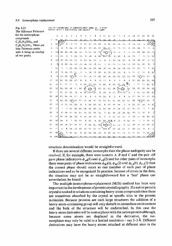
8.4 Isomorphous replacement 265
Fig. 8.23.The difference Pattersonfor the isomorphouscompoundsC3H5N2ONa2 andC3H5N2OA12. There arefour Patterson peakswith A being an overlapof two peaks.
FACTOR CONVERTING TO DENSITY/UNIT AREA IS 1.5705OUTPUT WITH Y HORIZONTAL AND ORIGIN TOP LEFT
0
1
2
3
4
5
6
7
8
9
10
11
12
13
15
16
17
18
19
20
21
22
23
24
0
100
43
-1
13
12
12
9
12
13
8
10
11
12
11
10
8
13
12
9
12
12
13
-1
43
100
1
2
16
14
15
8
7
9
11
13
11
11
11
13
11
9
7
8
15
14
16
2
2
Tl
< 4.
. 9.
. 14.
. 9.
. 16.
. 10.
. 7.
. 14.
. 22.
. 21.
. 13.
. 13.
. 13.
. 21.
. 22.
. 14.
. 7.
. 10.
. 16.
. 9.
. 14 .
. 9.
4 .
\\n
3
1 4
12.
14 .
10.
7 .
14.
11.
13.
23.
24.
12.
15.
12.
24.
3O23.
13.
11.
14.
7 .
10.
14 .
12.
14
4
12
11.
13 .
14.
15.
14.
10.
10.
c'17.
5.
11.
5.
17 .
26.
13.
10.
10.
14 .
15.
14.
13.
11.
1?
5
8
8.
10.
11 .
11.
9.
12.
12.
4 .
13.
8.
4 .
16.
4.
8.
13.
4.
12.
12.
9.
11.
11.
10.
8.
a,
6
10
12.
13.
9.
9.
10.
14 .
16.
9.
12.
8.
20.
2 0 ^
8 .
12.
9.
16.
14 .
10.
9.
9.
13.
12.
in
7
7
11 .
15.
11.
13.
16.
13.
14.
14.
14.
9.
27.
•27'
9 .
14.
14.
14.
13.
16.
13.
11.
15.
11.
"7
8
12 .
13.
11.
6.
12.
15.
16.
15.
12.
5.
13 .
28.
13 .
5 .
12.
15.
16.
15.
12.
6.
11.
13.
12.
1
9
1 8
10.
21.
10
1 4
6.
?A*33'' 54T
15
6.
11.
14.
10.
10.
8.
8.
13.
8.
8 .
10.
10.
14.
11.
6.
15.
-29:
6.
7 .
10.
6.
10.
13.
12.
15.
12.
13 .
10.
6.
10.
7 .
6.
11
1 8
10.
-21-
" 1 5 .
6.
11.
14.
10.
10.
8.
8.
13 .
8.
8 .
10.
10.
14 .
11.
6.
29^15 A
21.^29r
10.
18 ,
6.
-14^
)33N«
• 21*.
10.
18 •
12
15
12 .
13.
11.
6.
12 .
15.
16.
15.
12.
5.
13 .
28.
13 .
5 .
12.
15.
16.
15.
12 .
6.
11.
13 .
12.
13
7
11 .
15.
11.
13 .
16.
13 .
14 .
14.
14.
9.
27.
^50 .
N.
27r
9 .
14.
14 .
14 .
13 .
16.
13.
11.
15.
11.
14
10
12 .
13 .
9.
9.
10 .
14.
16.
9.
12.
8.
• 20 r
8 .
12 .
9 .
16 .
14.
10.
9.
9 .
13 .
12.
in
15
8
8.
10.
11.
11 .
9.
12 .
12.
4.
13 .
8.
B,16.
•* 4.
8 .
13 .
4 .
12 .
12 .
9.
11.
11 .
10.
8.
8-v
16
1 7
11.
13.
14.
15.
14.
10.
10.
13 .
26.
17.
5.
11.
5.
17.
26.
13.
10.
10.
14 .
15.
14 .
13 .
11 .
1?
17
1 4
12.
14 .
10.
7 .
14 .
11.
13.
23 .
24.
12.
15.
12 .
3 3<
23.
13 .
11.
14 .
7 .
10.
14.
12.
14
18
1 7,
4.
9.
14.
9.
16.
10.
7 .
14 .
»22.
21.
13.
13 .
13 .
»22.
14.
7.
10.
16.
9.
14 .
9.
4 .
•n
19
AI2.
16.
14.
15.
8.
7 .
9.
11.
13.
11.
11.
11.
11.
9.
7 .
8.
15.
14.
16.
2.
2 2 >
20
i no
-l
• 13
12
12
9
12
13
8
10
11
12
11
8
13
12
9
12
12
13
-1
*43"
structure determination would be straightforward.If there are several different isomorphs then the phase ambiguity can be
resolved. If, for example, there were isomers A, B and C and the pair ABgave phase indications (j)AB(l) and (j)AB(2) and for other pairs of isomorphsthere were pairs of phase indications (j)BC(^\ <t>BcQ) anc* <I>CAW> <t>cd?) ^ e n
the correct phase should occur as one member of each pair of phaseindications and so be recognized. In practice, because of errors in the data,the situation may not be so straightforward but a 'best' phase cannevertheless be found.
The multiple-isomorphous-replacement (MIR) method has been veryimportant in the development of protein crystallography. If a native proteincrystal is soaked in solutions containing heavy-atom compounds then theseare sometimes absorbed by the crystal at specific sites in the proteinmolecules. Because proteins are such large structures the addition of aheavy-atom-containing group will only disturb its immediate environmentand the bulk of the structure will be undisturbed. In this case theheavy-atom derivative will be isomorphous with the native protein although,because some atoms are displaced in the derivative, the iso-morphism may only be valid to a limited resolution - say 2-3 A. Differentderivatives may have the heavy atoms attached at different sites in the

266 The determination of crystal structures
Fig. 8.24.A Fourier summation,derived from theheavy-atom positions inC3H5N2ONa2 andC3H5N2OA12, whichshows the positions ofthe light atoms. Spuriouspeaks are marked Sp.
FACTOR CONVERTING TO DENSITY/UNIT AREA IS 0.0483OUTPUT WITH Y HORIZONTAL AND ORIGIN TOP LEFT
17
18
19
20
21
22
23
24
9 10 11 12 13 14 15 16 17 18 19 20
8 13
9 7
10 9
11 12
12 -18
13 5
14 6
15 11
16 0
3
13
0
15
9
1 5 .
4 .
• 6.\
/ 1 6 .
9 .
16.
11.
3
1 0 .
- 8 .
1.
- 2 .
7 .
8 .
6 .
7.
2.
7.
2 .
4 .
- 1 .
-7
1 2 .
5 .
c20.
8.
1 8 .
3 .
it4 .
1 .
27 . /I
2 2 :\
3 .
2 .
1 .
- 6 .
4 .
4 .
3 .
26.^
2O.\
l n
3 .
34 .
\ V
2 0 .
- 5 .
2 .
14.^-
3 . 6
*" •«41,<--34
y"^6 7* 7
2 0 .
8 .
5 .
1 7 .
•69\^58.\ ^ _ >
- 1 .
6 .
-2.
7 .
0.
——^
1 .
7 .
- 4 .
3 .
0 .
1 3 . 9.
Z56v
* ir"
1 6
5
" 1 1
1
14
- 6
\ 6
ll 3
1
5
3
-3
1
5
2
-. 12
2
7 1 0
. 7
. 21
. 18
. 16
12
. 8
. 12
. -23
. 3
. 5
. 4
. 6
. 2
. 12
. 6
. 7
. 10
. 0
. 1
. 9.
. 2C ^I
. 21)\
. 12.
• &
. 10 .
1.
. - 1 6 . -
. 15 .
4 .
. 15 .
. 25. ' v
. 3 .
. 12.
. 3 .
. - 1 .
9 .
7 .
. 8.
- 1 .
r r
8
- ! 2
2 5 — 13
7 2 \
i .
3 .
1 2 .
3 .
- 3 .
2 0 -
3 0 \
1 4 .
1 .
8 .
N16
*18
3
9
20
1
9
^59
24
\
3
1
. 1 4 .
\ 9.
< 0.
. 1 3 .
. 3 .
. 0.
11
. 6.
. 5 .
. - 1 8 .
. 12.
. 9.
J\ 7
' 8.
• 3 1 /
. 1 1 .
4 .
- 1
2
6
2
7
6
8
7
- 2
1
- 8
1 0
3
1 1
16
9
16
6
4
1 5
. 20 O 4<~~55-s 14
26 i (JX\ ) I. 2 6 .
. 3 .
4 .
4 .
. - 6 .
. 1 .
. 2 .
3
. 22 .
Sp '
. 4 .
• v. 3 .
. 18 .
. 8 .
. 20 .
. 27 .
. 5 .
. 12 .
10
S 1 3 ^
0.
7.
- 2 .
6 .
- 1 .
2.
*—*v
20.
3 .
ni.
3 .
18
- 9
0
3
- 4
7
1
10
2 .
5 .
1 .
- 3 .
3 .
5 .
1
- 1 7 "
5 .
- 2 2 .
-V.20.
- 6 .
4 1 .- • • s
~*3*"
/ ' 6 .
- 6 .
1 4 .
1 .
\l4.
1 1 .
5 .
16.
7.
34.
6.
7 .
1 .
0 .
10.
7 .
6.
1 2 .
2 .
6.
4
5 .
3 .
- 2 3 .
1 2 .
8 .
1 2 .
1 6 .
18.,
21 \
7 .
10.
0 .
2 .
12.
3
8
7
9
-1
3
12
3
Sp
4 .
1 5 .
-16.
1 .
1 0 .
3 9 '
/ J-
1 2 .
21(
20 V
1 2 .
9.
-2
8
1
. 1
3
3 0 / 7 ^
2 3 ^
2 0
€- 3 .
3 .
-12 .
3 .
1 .
" 3 ^
7 2 )
^ 8 -
259 .
1 .
- 20 .
9 .
3 .
1 0 .
La.
26. 13 .
4s.
- 1 .
-1
8 .
4
1 1
^.21
" 8
>3
/ 7
9
12
- 1 8
5
6
1 1
0
3
13
0
1 9
7
14
protein; each derivative gives two possible values for the phase of theprotein but with several different derivatives a unique 'best' phase for theprotein can usually be found.
A general approach to combining information from MIR experiments,considered in the form of a number of SIR experiments, from each of whichthere is a phase ambiguity, was suggested by Blow and Crick (1959). Byconsidering the probable errors of measurement each experiment gives aprobability curve for the phase looking something like that in fig. 8.25. Thepeaks of the map correspond to the ambiguity and the spread around eachof the peaks is related to the probable errors of measurement. For veryprecise measurements the two peaks become sharp and narrow; if themeasurements are very poor then the probability may vary little over thewhole 2TI range. Again, if the A0 associated with the ambiguity is small thenthe two peaks may coalesce to give a unimodal distribution. Curves fromfour different experiments and the product of the four curves are shown infig. 8.26. It will be seen that, although each individual experiment gives arather diffuse curve the overall probability curve can define the phase quitewell.
A complete review of methods dealing with multiple isomorphousreplacement (MIR) has been given by Woolfson and Fan (1995).

8.5 The application of anomalous scattering 267
Fig. 8.25.A Blow and Crickprobability curve for aphase fromsingle-isomorphous-replacement (SIR) data.
P(0(h))
Fig. 8.26.(a-d) Crick and Blowprobability curves fromdifferent pairs ofisomorphs multipliedtogether to give (e) aunimodal probability
P(0) (a)
8.5 The application of anomalous scattering
In §6.6 anomalous scattering was described as a phenomenon whichinfluences the intensities of X-ray reflections and causes a breakdown ofFriedel's law so that \Fh\ / I F_h |. We shall now see how to exploit thisdifference to solve crystal structures.
In fig. 8.27(a) there is shown the way that Fh may be decomposed into the
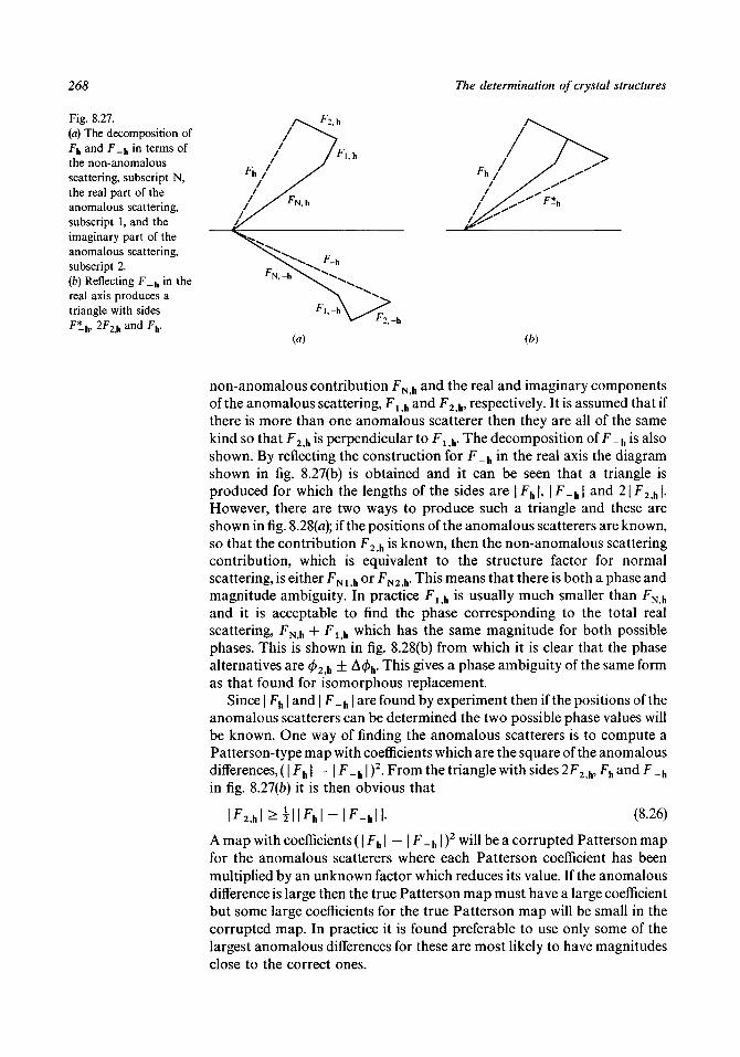
268 The determination of crystal structures
Fig. 8.27.(a) The decomposition ofFh and F _ h in terms ofthe non-anomalousscattering, subscript N,the real part of theanomalous scattering,subscript 1, and theimaginary part of theanomalous scattering,subscript 2.(b) Reflecting F _ h in thereal axis produces atriangle with sidesF*_h, 2F2,h and Fh.
N,h
(a) (b)
non-anomalous contribution FN h and the real and imaginary componentsof the anomalous scattering, Flh and F2 h, respectively. It is assumed that ifthere is more than one anomalous scatterer then they are all of the samekind so that F2h is perpendicular to Flh. The decomposition of F_h is alsoshown. By reflecting the construction for F_h in the real axis the diagramshown in fig. 8.27(b) is obtained and it can be seen that a triangle isproduced for which the lengths of the sides are | Fh|, \F_h\ and 21F2 h|.However, there are two ways to produce such a triangle and these areshown in fig. 8.28(<z); if the positions of the anomalous scatterers are known,so that the contribution F2h is known, then the non-anomalous scatteringcontribution, which is equivalent to the structure factor for normalscattering, is either F N 1 h or FN2fh. This means that there is both a phase andmagnitude ambiguity. In practice Flh is usually much smaller than FN h
and it is acceptable to find the phase corresponding to the total realscattering, FN h + Flh which has the same magnitude for both possiblephases. This is shown in fig. 8.28(b) from which it is clear that the phasealternatives are </>2 h ± A(/>h. This gives a phase ambiguity of the same formas that found for isomorphous replacement.
Since | Fh | and \F_h\ are found by experiment then if the positions of theanomalous scatterers can be determined the two possible phase values willbe known. One way of finding the anomalous scatterers is to compute aPatterson-type map with coefficients which are the square of the anomalousdifferences, (| Fh \ — \ F_h \ )2. From the triangle with sides 2F2 h, Fh and F_h
in fig. 8.27(b) it is then obvious that
\ F 2 M \ > ± \ \ F h \ - \ F _ h \ \ . (8.26)
A map with coefficients (| jFh | — | F_ h | )2 will be a corrupted Patterson map
for the anomalous scatterers where each Patterson coefficient has beenmultiplied by an unknown factor which reduces its value. If the anomalousdifference is large then the true Patterson map must have a large coefficientbut some large coefficients for the true Patterson map will be small in thecorrupted map. In practice it is found preferable to use only some of thelargest anomalous differences for these are most likely to have magnitudesclose to the correct ones.

8.5 The application of anomalous scattering 269
Fig. 8.28.(a) If the positions ofthe anomalousscatterers are known, sothat F2,h ^s known inboth magnitude andphase then finding thenormal structure factorFNj, gives an ambiguityboth in magnitude andphase.(b) Finding the totalreal scattering givesonly a phase ambiguity. \Fh\
(b)
We now illustrate this process using the synthetic structure C3H5N2ONa2,shown earlier in fig. 8.17 where the Na atoms are the anomalous scatterers.Table 8.6 shows the structure factors calculated for Fe Kax radiation(A = 1.936 A) for which, for Na,/X = 0.186 and/2 = 0.196. This table wasproduced by STRUCFAC which contains a facility for including anomalousscattering. The anomalous components of the scattering factor are, in fact,very small and normally, in a real case, the anomalous scatterers would beheavier elements with the wavelength tuned to give large anomalous effects.For example, if Co Kax radiation (X = 1.789 A) was used with Fe as theanomalous scatterer then/j = — 3.331 and/2 = 0.490. However, since weare dealing with idealised calculated structure factors we can use the verysmall differences in | Fh | and | F_h | seen in table 8.6 for our illustration.
The output file from STRUCFAC was used as the input file forANOFILE, given in appendix IX. This gives an output data file which canbe input to FOUR2 to give the required anomalous-difference Pattersonmap, which is shown in fig. 8.29. Only one-quarter of the largest anomalousdifferences are used, the remainder being made equal to zero by ANOFILE.Ideally the map should show only the vectors linking the anomalousscatterers but, since the coefficients of the map are not those of a truePatterson function the map obtained is somewhat corrupted. Comparingfig. 8.29 with fig. 8.23 we can see that peaks A, B and C appear but B and Care slightly displaced and that there are also smaller false peaks present. It ispossible to interpret fig. 8.29 although the coordinates found will be slightlydifferent from the true coordinates. It should be noted that the X-raywavelength used here for anomalous scattering, chosen to give reasonablevalues of/t and/2, also gives lower resolution for fig. 8.29 than for fig. 8.23,for which Cu Ka radiation (X = 1.542 A) was used.
Having determined the positions of the anomalous scatterers, thequantities F2h for different h can be calculated so defining the phasealternatives for each reflection and then a double synthesis can becalculated as given in equation (8.25). Another interesting way of resolving

270 The determination of crystal structures
Table 8.6. Structure factors for the non-centro symmetric structure C3H5N2ONa2 with anomalousscattering by the sodium atoms
PHI is the phase angle in degrees. The anomalous components of the scattering factor are/j =0.186 and/ 2 = 0.196.
h- 8
7- 7
6-6
6- 5
5- 4
4- 4
4_ 2
3- 3
2- 2
2- 2
1- 1
1- 1
000001
- 11
- 12
- 22
- 22
- 33
- 33
- 44
- 44
- 55
- 56
- 66
- 67
- 78
- 8
k1
- 13
- 13
- 42
- 31
- 24
- 52
- 35
- 13
- 46
- 13
- 4602
-35
- 61
-24
- 50
- 13
- 4602
- 3502
- 3502
- 30
- 13
- 41
- 201
F4.87
14.336.84
14.4615.27
8.6114.7014.6314.80
6.1211.9512.0215.92
8.1911.6416.3918.44
9.817.715.158.97
29.054.50
124.7519.92
0.000.00
14.104.64
29.4828.5915.6117.7616.3918.44
9.817.712.97
15.928.19
11.6416.69
6.1227.2911.68
2.2814.7014.6315.5314.4615.27
8.6114.1314.0715.71
4 R7
PHI8 1 .
-125 .- 7 0 .133.- 3 1 .150.
1 .140.
-158.4 5 .1 6 .
- 9 2 .175.- 1 1 .
-150 .159.
- 8 .- 7 5 .166.-53 .-35.
5 3 .-4 .
0 .106.
0 .0 .
168.-128.
168.- 5 1 .-32.
2 .- 2 1 .172.- 7 5 .166.
-180 .175.169.
3 0 .-180 .
-45.-165.
-84.0 .1 .
- 4 0 .-178 .
-47 .149 .150.- 5 3 .- 2 0 .
-177.9 9 .
h8
- 77
- 66
- 55
- 54
- 44
- 33
- 33
-22
-22
- 11
- 1100001
- 11
- 11
-22
-22
-23
- 33
- 34
- 44
- 45
- 55
- 66
- 67
- 77
- 8
k- 1
2- 3
2- 3
1-2
4- 1
3- 4
1- 2
4- 5
2- 3
5- 6
2- 3
5- 6
1-2
4- 5
0- 1
3- 4
602
- 35
- 61
-24
- 51
-24
- 51
-2402
- 30
- 130
F4.87
13.916.84
18.0415.8637.6014.97
5.5115.3026.9211.9430.4716.22
3.6811.7032.5318.632.868.04
29.128.97
15.644.490.00
20.1212.23
0.0017.82
5.158.97
29.054.50
17.7632.5318.63
2.868.04
30.4716.22
3.6811.7014.80
6.1211.9512.0237.6014.97
5.5015.5318.0415.86
8.7114.33
6.8415.71
PHI- 8 1 .
2 5 .7 0 .
-68.3 5 .
171.1 .
141.161.- 1 2 .- 1 6 .134.
-174.7 0 .
156.125.
1 1 .5 3 .
-159.-166.
3 5 .-146.
4 .0 .
-104.-134.
0 .0 .
127.145.
5 3 .- 4 .
2 .125.
-169.-127.-159.
-46.-174 .
7 0 .-24.
2 2 .4 5 .1 6 .8 8 .- 9 .
1 .141.
-178.-68.
-145.-180.
5 5 .110.
-177 .
h- 7
7- 6
6- 6
5- 5
5- 4
4- 4
3- 3
3- 2
2- 2
2- 1
1- 1
100000
- 11
- 11
- 12
- 22
- 23
- 33
- 34
- 44
- 45
- 55
- 56
- 66
- 77
- 78
k1
- 21
- 24
- 13
- 42
- 35
- 13
- 41
- 24
- 51
- 24
- 50
- 13
- 4602
- 35
- 61
- 24
- 50
- 13
- 40
- 13
- 40
- 13
- 41
- 2402
- 31
F14.1314.0714.3518.12
8.3437.1814.63
5 .616.12
27.2911.6830.85
8.183.19
16.0432.48
9.973.374 .64
29.4828.5915.61
124.750 . 0 00 . 0 0
12.0714.5217.8229.12
8.9715.64
4.4916.0432.48
9.973.372.97
30.858.183.19
16.6915.302 6 . 9 211.94
2 . 2 837.1814.63
5 .6114.3518.12
8.348.71
13 .916.844.87
PHI127.-20.
-131 .6 9 .
-147.-169.-140.-136 .
-45 .1 5 .9 6 .
-131 .1 1 .
- 72 .-158.-124 .
7 8 .-49 .
5 2 .168.- 5 1 .148.
0 .0 .0 .
131.-162 .
0 .-166.-145 .
3 4 .4 .
2 2 .-124 .
7 8 .131.
-180 .4 9 .
-169 .- 7 2 .
-180 .-19 .168.-16 .
0 .1 1 .4 0 .
-136 .4 9 .6 9 .
-147.-180 .
2 5 .-110.
-99 .

8.5 The application of anomalous scattering 271
Fig. 8.29.Theanomalous-differencePatterson map forC3H5N2ONa2.
FACTOR CONVERTING TO DENSITY/UNIT AREA IS 0.0009OUTPUT WITH Y HORIZONTAL AND ORIGIN TOP LEFT
9 10 11 12 13 14 15 16 17 18 19 20
0
1
2
3
4
5
6
7
8
9
10
11
12
13
14
15
16
17
18
19
20
21
22
23
24
100.
63
3
-12
5
5
-6
0
4
-15
-31
-18
-4
-18
-31
-15
4
0
-6
5
5
-12
3
63
100
-14 .
5.
11.
4.
0.
-3.
-17.
-27 .
-21.
-14.
-21.
-27.
-17.
-3.
0.
4.
11.
5.
-14.
-7.
-10.
-9.
3.
2Q,
1.
-14.
-11.
-5 .
-12.
-19.
-12.
-5.
-11.
-14 .
1.
20.
20.
3.
-9.
-10.
C
-1.
11.
1.
-6.
xll.
•18.
-4.
-18.
4.
r
V8.
-8.
8.
2 *4*
-18.
-4.
N18.
1'11.-6.
1.
11.
-1.
17.
20.
-2.
-19.
-11.
0.
-9.
-13.
7.
"2*1N
~ 4.
-10.
4.
"~1.
-13.
-9.
0.
-11.
-19.
-2.
20.
17.
7.
-1.
-9.
-13.
-11.
-4 .
3.
5.
1.
-7
-15.
-18.
-15.
-7.
1.
5.
3.
-4.
-11.
-13.
-9.
-1.
7.
-13.
-20.
-3.
13.
7.
2.
17.
24'
3.
-15
-3.
10.
-3.
-15.
3.
24T
17"!"
2.
7 .
13.
-3.
-20.
-13.
-23.
-21.
4.
20.
3.
-12.
3.
ye.3.
-1
-1.
3.
•J.6.
3.
-12.
3.
20.
4.
-21.
-23.
-23
-6
7
2
-17
-27
-16
-4
1
q
42
" ^
"i1
-4
-16
-27
-17
2
7
-6
-23
.-15
. 18
. 17
. -6
.-15
. -6
. -2
. 0
. 8
11
V./-I
. 11
. 8
. 0
. -2
. -6
.-15
. -6
. 17
. 18
.-15
.-10.
.,'22.
\ 26.
. -4.
. -5.
. 14.
. 16.
. 10.
. 16.
12
.-19.
.-40.
.-19.
. 12.
. 16.
. 10.
. 16.
. 14.
. -5.
. -4.
-15.
^ 1 8 .
17/.
-6.
-15.
-6.
-2.
0.
8.
11
-1.
-10.
-1.
11.
8.
0.
-2.
-6.
-15.
-6.
.,2<f>17.
!,32.
.-10.
if.r15.
-23.
-6.
7.
2.
-17.
-27.
-16.
-4.
1.
9
-23 .
-21.
4.
20.
3.
-12.
3.
16.
3.
-1
30*""29N
k9"
1.
-4.
-16.
-27.
-17.
2.
7 .
-6.
-23.
V-21' ^1.
3.
16.
3.
-12.
3.
20.
4 .
-21.
-23.
-13.
-20.
-3.
13. -
7. -
2.
17.
€'3.
-15
A--15.
3.
24->
lV
2.
7
-1
-9
13
11
-4
3
5
1
-7
15
18
15
-7
1
5
3
-4
7. -11
13.-
-3.
-20.
-13.
13
-9
-1
7
. 17.
. 20.
. -2.
.-19.
.-11.
. 0.
. -9.
.-13.
7 .
21'\
. 4.
.-10.
4 .
. 21/
V. 7.. -13.
. -9.
. 0.
. -11.
.-19.
. - 2 .
. 20.
17.
9
-1
11
1
-6
11
18
-4
-18
4
"~ "8
-8
8
23-
"4
-18
-4.
18.
11.
-6.
1.
11.
-1.
-7 .
-10
-9.
3.
20,.
i<L1.
-14.
-11.
1 -5
-12.
-19.
-12.
' -5.
-11.
-14.
1.
20-
io_
3.
-9.
-10.
-7.
'4-7.
-14.
5.
^ 1 1 .
1J 4.
0.
-3.
-17.
-27 .
-21.
-14.
-21.
-27.
-17.
-3.
0.
N 4-
Al.5.
-14.
-7 .
\*—
-12
5
5
-6
0
4
-15
-31
-18
-4
-18
-31
-15
4
0
-6
5
5
-12
3
the phase ambiguity for one-wavelength anomalous scattering (OAS) byusing anomalous differences will now be described.
Let us write the scattering factor of an atom as
where the imaginary component is non-zero only for an anomalousscatterer and is the f2 of equation (6.80) and the real component for ananomalous scatterer, (fj)R, differs slightly from the non-anomalous valueand is the/0 +/ i of equation (6.80).
The structure factor of index h can now be written as
N N
Fh = Z (/j)*exP(27lih#r/) + J Z A/} exp(27tihT;).
The complex conjugate of Fh is given by
n = I (/;)*exP( - - i I A/) exp( -
(8.27)
(8.28)
The form of the second summation follows from the result that the complexconjugate of iei0 ( = i cos 0 — sin (/>) is — i cos 0 — sin 0 which can be

272 The determination of crystal structures
written as — ie"i<iP.From equations (8.27) and (8.28) we find
N
(/))i?exP(27lih#ri) + * Z A/} exp^Trih-r,.)
r N N -i
x Z (fj)R™P( ~ 27tih-r,.) - i £ Afj exp( - 27iih-r,.) . (8.29)
Similarly we find that
r N N • iI F.h |
2 = | ^ I (/^exrf - 27uh-r,.) + i £ 4/) exP( " ^ ^ Jx [ £ (/^exp(27iih-rj) - i £ Afj exp(27iih-ri)]. (8.30)
U = l 7=1 J
By combining equations (8.29) and (8.30) one obtains
l^hl2 + l^-hl2 = 2 Z Z WRWR + A/fcA/)}cos{27ih-(r, - r )} (8.31)
and
\f |2 _ | p_ |2 _ 2 V V M / / / ) (/.) — Af(f) } sin{27ih#(r — r-)}.
(8.32a)
If in equation (8.31) we write (^c)h = \{ \ Fh \2 + | F_h |2} then it is clear
that (i/ c)h is the hth Fourier coefficient of a function which has peaks atrk — Tj. These peaks will have Fourier transforms which, at the point inreciprocal space corresponding to the index h, have values (fk)R(fj)R + AfkAfj.This peak will be like a normal Patterson peak except that when one orboth of the atoms is an anomalous scatterer the peak is very slightlymodified in weight and form. The Fourier synthesis with V~l(\j/\ asFourier coefficients gives a function Pc (u) which will thus be similar to anormal Patterson synthesis obtained with non-anomalous scattering dataexcept at points corresponding to the vectors involving anomalous scatterers.
Equation (8.32a) is the basis of a much more interesting function firstdiscussed by Okaya, Saito and Pepinsky (1955). It simplifies our considerationof this function if it is assumed that there is only one anomalous scatterer inthe unit cell, i.e. the one for which; = 1. Equation (8.32a) then becomes
N
I ^h I2 ~ I F-h I2 = 2 Z Afi(fk)R sin{27ih-(rfc - r j } . (8.32b)
If we write (ij/s\ = \Fh\2 - \F _h\
2 then (i^s)h = - 0As)-h-l t should nowbe clear that (^s)h is the Fourier coefficient of an odd function Ps(u) whichwill have a peak corresponding to the transform of Afx(fk)R at (xk — r x) and apeak corresponding to the transform of — Afx{fk)R at —(rk — r1). Thefunction Ps(u) is given by
). (8.33)

8.5 The application of anomalous scattering 273
Fig. 8.30.The synthetic structure
This function will have peaks from an anomalous scatterer, say atom m, toany other atom, say atom n, of weight approximately proportional to AfmZn
and peaks from atom n to an anomalous scatterer, atom m, of weight-AfmZn. The significance of this anti-centrosymmetric function is that itnot only gives a pattern of peaks, positive and negative, which can be usedto solve the structure but the absolute direction from an anomalousscatterer to other atoms is clearly indicated. Thus if the positive directionsof the axes with respect to the crystal are defined and the record of thereflection of index h is distinguished from that of index — h then the absoluteconfiguration of the crystal structure can be determined. When a molecularstructure exists in enantiomorphic forms then, if it contains an atom forwhich a suitable wavelength can be found to give anomalous scattering, theabsolute configuration of the enantiomers can be determined. Withoutanomalous scattering the diffraction patterns of the two forms are identicaland they cannot be distinguished.
To illustrate the principle of the Ps(u) function there is shown in fig. 8.30 ahypothetical structure in space group pi with the sulphur atom acting asthe anomalous scatterer. Anomalous structure factors were calculatedusing STRUCFAC and the output was used as input for PSCOEFF(appendix X). This program produces an output file with amplitudes andphases which, used as input for FOUR2 gives a Ps-function map. The map,reproduced in fig. 8.31, shows positive peaks from the anomalous scattererto other atoms and negative peaks in the reverse directions. Because twocarbon atoms are nearly centrosymmetrically disposed about the sulphuratom the positive and negative peaks related to these two atoms partiallycancel each other - although the peaks can still be clearly seen.
Synchrotron sources of X-rays (§ 5.8) can give radiation tuned to aparticular wavelength and increasingly this is being used to make anomalousscattering measurements for a given structure at several different wavelengths.The anomalous scatterers have values offx and/2 which depend on theX-ray wavelength and if the wavelengths used are tuned to be close to anabsorption edge for the anomalous scatterer then there will be largechanges in the anomalous components of the scattering factor (see fig. 6.17).Many-wavelength anomalous scattering (MAS) overcomes the phaseambiguity of OAS (Woolfson and Fan, 1995).
Anomalous scattering can also be used to resolve the ambiguity of phase

274 The determination of crystal structures
Fig. 8.31.The Ps-function mapfor C5H9S. Positivecontours are drawnwith solid lines andnegative contours withdashed lines.
FACTOR CONVERTING TO DENSITY/UNIT AREA IS 1.1507OUTPUT WITH X HORIZONTAL AND ORIGIN BOTTOM LEFT
0
20 0
19 -10
18 -4
17 -12
16 -51
15 -76
14 -50
13 -5
12 10
11 3
10 0
9 -3
8 -10
9 10 11 12 13 14 15 16 17
>fl. 1fi
- 2 .
- 1 1 .
- 1 2 .
- 2 5 .
- 3 4 .
- 1 6 .
6 .
- 1 .
- 2 3 .
- 2 8 .
- 1 8 .
- 1 1 .
1 4 .
^66""
v^„>
1 9 .
4 .
18.
1 7
-11
-13
- 7
- 1 5
-27
-16
- 2
- 2 7
- 2 5
- 1
3 2
2 6
- 8
- 1 6
- 2
- 2 2
-74 £78
-atei- 1 8
1
) 7°
9
- 2
7
'<-5~7
- 6
5
- 4
- 2
2
- 2
- 3
- 3
. - 1 5 . - V 5 9 > - 6 1 .
. 2T*
. - 2 1
. - 1 2
. - 1
s;27
*-48
?M. 14
. 20
. 5
. -1
. -3
. -4
. 0
. -2
- W .
1 2 .
- 2 7 .
-eeZ-g's.
717.
- 1 0 .
4 .
- 1 4 .
-22>-4St%30\
0 .
- 6 .
- 6 .
5 .
8 .
6 .
5 .
_3 #
- 1 5 .
- 1 2 .
- 7 .
-7 .
- 1 .
- 6 .
- 4 .
- 3 .
- 3 .
2 .
0 .
- 1 2 .
- 1 7 .
- 8 .
- 2 .
1 .
0 .
6 .
4 .
- 2 .
6 .
2 0 .
1 6 .
2 .
4 .
1 8 .
- 2 .
- 1 1 .
- 3 .
- 3 .
-18.
7 2 4-- 8 .
5 .
1 .
- 4 .
- 2 .
- 5 .
- 1 3 .
- 5 .
1 7 .
2 1 .
7 .
4 .
-2
-17
- 2 4
- 1 3
-7
-16
- 2 1
- 9
1
- 5
- 1 6
- 1 7
- 1 7
- 2 3
- 2 1
- 6
4
- 1
- 4
- 5 .
- 1 6 .
- 1 6 .
2 .
12.
3 .
- 5 .
6 .
1 3 .
0 .
- 1 3 .
- 6 .
5 .
- 3 .
- 1 2 .
- 2 .
1 6 .
1 6 .
5 .
4
1
- 4
6
21
23
17
17
16
5
- 1
9
2 1
16
7
13
2 4
17
2
- 4 .
-7 .
- 2 1 .
- 1 7 .
5 .
13 .
5 .
2 .
4 .
- 1 .
- 5 .
8 .
2 4 .
1 8 .
3 .
3 .
1 1 .
2 .
- 1 8 .
- 4 .
- 2 .
- 1 6 .
- 2 0 .
- 6 .
2 .
- 4 .
- 6 .
0 .
- 1 .
2 .
30 .
1 4 .
-4 .
1 0 .
1 7 .
- 1 .
8.
17.
1 2 .
0.
- 2 .
3 .
3 .
4 .
6 .
1 .
7 .
91^.
2 7 T
- 1 2 .
1 9 .
ii
i.
12.
1 5 .
3 .
- 5 .
- 6 .
- 8 .
- 5 .
6 .
6 .
0 .
- 5 1 .
- 1 4 !
2.
0.
4 .
3 .
1.
- 5 .
- 2 0 .
- 1 4 .
2 4 .
48 .1
2 7 .
1 .
\ 1 2 .
/21.
-21.
Sl 5.
J).
3 .
3 .
2 .
- 2 .
2 .
4 .
- 5 .
6 .
-7 . -
2 .
- 9 . -
- 4 1 . -
-50<1\ V
-26 . v -
- 1 . -
1 8 .
5 7 ^ 5 ^
rfnnOsN
2 2 .
2 .
1 6 .
8 .
- 2 6 .
'-'32.
1 .
2 5 .
<11 .
2 .
1 6 .
2 7 .
1 5 .
7 .
13 .
11 .
18 .
-4 .
1 9 .
72*
\
11 .
1 8 .
\
Li
- 6
16
3 4
2 5
12
1 1
2
-10
-4
- 1 2
~ 5 >
/
10
3
0
- 3
- 1 0
5
50,
i12
4
10
n
which results from the use of a single pair of isomorphous compounds. If thesimplest case of a single i-r atom is taken then the phase ambiguity is shownin fig. 8.32. When X-rays are used for which the i-r atom Z scattersanomalously, a component Afz is added to the scattering factor (ignoringthe change in the real part) and the new structure factor is shown in fig. 8.32as OQ or OR depending on whether it was originally OQ or OR. Since OQand OR' will have different magnitudes it will be possible to distinguishwhich of the phases is the correct one.
Another way of combining SIR and OAS is by the probability curvemethod illustrated earlier in fig. 8.26. Although the atomic positions for bothisomorphous replacement and anomalous scattering are the same, thecentral phases of the phase ambiguities, 0xh and (/>2?h, will differ by it/2 so thatthe multiplication of the probability curves will not give a symmetrical result.
8.6 Inequality relationships
In 1948, Harker and Kasper showed that inequality relationships existedbetween the structure factors and that these relationships could occasionallylead to definite information about the phases of structure factors. To derivethese relationships, the Cauchy inequality can be used. This is
N
I K-I (8.34)
where a} and b} can be real or complex quantities.

8.6 Inequality relationships 275
Fig. 8.32.The resolution of thephase ambiguity fromisomorphousreplacement withanomalous scattering.
We shall apply this inequality to derive relationships between unitarystructure factors. The assumption will be made that the unitary scatteringfactors, the n's remain constant over reciprocal space. If the structurecontains atoms of equal weight, or nearly so, this assumption will bejustified; if there are heavy atoms present then, since their scattering factorsfall off more slowly with sin 6 than do those of light atoms, the assumption isnot really valid.
Consider the unitary structure factor
h = X nj exp(27tih-r;). (8.35)
Taking a^ = y/rij and bj = ^Jnj exp(27iihTJ) then from Cauchy's inequalitywe find
(8.36)
Since
|exp(27iihT;)| =
and
N
Tj) + i sin(27ih*r7-) | =
inequality (8.36) gives
(8.37)

276 The determination of crystal structures
This is a fairly obvious inequality and not a useful one, since by the veryway in which Uh is defined it must be true. However more useful results areobtained as soon as we take account of the presence of symmetry elements.
Thus for a centre of symmetry we have
Uh = £ n,.cos(27ih-r,.). (8.38)7 = 1
Putting cij = y/rij and bj = v/^cos(27ih-rJ) we find
ul < I nj x I ";cos2(27ih-r,.). (8.39)7 = 1 7 = 1
Now
N N N
£ njCOS2(2nh'Tj) = \ £ nj + \ £ n</cos(27c2hT</.)7 = 1 7 = 1 7 = 1
so that
^ h ^ l + ^ h ) . (8.40)
This inequality can be used to give the sign of £/2h; if it is written in the form
^2h >2Ul-l (8.41)
this can be seen a little more easily. If | Uh \ and | t/2ll I are both sufficientlylarge then one can show that (72h must be positive. Thus if | Uh \ = 0.6 and| £/2h| = 0.5 then, since from inequality (8.41)
U2h ^ - 0.28,
it is clear that U2h must be positive since the negative sign for Ulh wouldcontravene the inequality.
Let us now see what inequalities result from having a twofold axis.Atoms will occur in pairs with coordinates (x, y, z) and ( — x,y, —z) and theunitary-structure-factor equation appears as
Um = £ nj exp(27ii/c^)cos{2Ti(/i^ + Izj)}. (8.42)7 = 1
For dj = y/rij exp(2nikyj) and bj = y/njCOs{2n(hXj + Izj)} this gives
\Uhkl\2^^l + U2h<oai). (8.43)
This inequality can be very useful. The fo-axis projection is centrosymmetricand it is possible to determine the sign of a large structure factor V2K02l ifany of the structure factors Uhkl has a sufficiently high magnitude.
If, together with the twofold axis, there is a centre of symmetry then theunitary-structure-factor equation has the form
N
Uhkl = Z ";cos(27tfcy;)cos{27t(/zx; + IZJ)}. (8.44)7 = 1
This can lead to two different inequality relationships depending on the
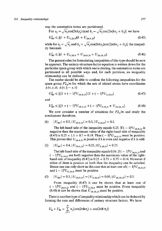
8.6 Inequality relationships 277
way the summation terms are partitioned.
For aj = y/njCOs(2jikyj) (and bj = y/rij cos{2Ti(hXj + Izj)} we have
U2hkl < *(1 + l / 0 , 2 W X l + t/2*.o.2i) (8-45)
while for a,. = ^/n^ and fey = ^/rijCOs(2nkyj)cos{2n(hXj + /z,)} the inequal-ity becomes
U2hkl ^ i ( l + £/0,2*,0 + l/2*.O.2I + ^ 2/,,2*,2/)- (8-46)
The general rules for formulating inequalities of this type should be nowbe apparent. The unitary-structure-factor equation is written down for theparticular space group with which one is dealing, the summation terms arepartitioned in all possible ways and, for each partition, an inequalityrelationship can be deduced.
The reader should be able to confirm the following inequalities for thespace group Pljm for which the sets of related atoms have coordinates±(x,y,z), ±(x,±-y,z):
U2hkl < i{l + ( - 1)*£/2*,O,2/}{1 + ( - l?U0f2ht0} (8.47)
and
UL < i U + ( " l)**Vo,2I + ( " l)*t/o,2*,o + U2ht2kai}. (8.48)
We now consider a number of situations for P2Jm and study theconclusions therefrom.
(1) | Uhkl | = 0.5, | U2Mt2l | = 0.3, | UoaM | = 0.1.
The left-hand side of the inequality equals 0.25. If ( — l)kU2h02l *s
negative then the maximum value of the right-hand side of inequality(8.47) is 0.25 x 1.1 x 0.7 = 0.19. Thus ( - l)kU2htOf2l must be positive.This proves that V2h02l is positive if k is even and negative if k is odd.
(2) | Uhkl | = 0.4, | U2hMl | = 0.25, | UoaKO | = 0.25.
The left-hand side of the inequality equals 0.16. If ( — l)kU2hiOt2l and( — i)kUOt2ktO are both negative then the maximum value of the right-hand side of inequality (8.47) is 0.25 x 0.75 x 0.75 = 0.14. However ifeither of them is positive or both then the inequality can be satisfied.Hence one can only show in this case that at least one of ( — l)kU2h0 2l
and ( - l)*l/o,2fcfo m u s t be positive.
(3) | Uhkl | = 0.5, | t / 2 M t 2 I | = | U0Mt01 = 0.05, | U2K2K2l | = 0.3.
From inequality (8.47) it can be shown that at least one of( — l)kU2h0 2l and ( — l)k£/o,2fc,o must be positive. From inequality(8.48) it can be shown that U2K2k2l must be positive.
There is another type of inequality relationship which can be deduced byforming the sum and differences of unitary structure factors. We have
N
Uh + UW= ^ ny{cos(27ih-ri) + cos(27ih/-rJ-)}
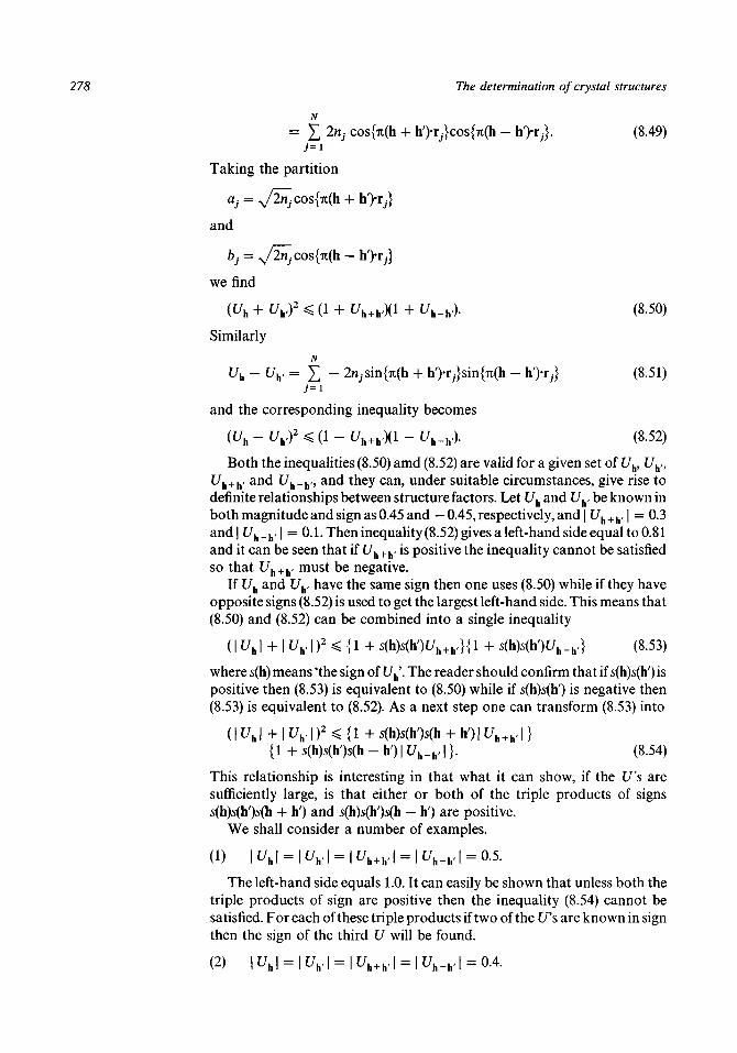
278 The determination of crystal structures
N
= £ 2nj cos{7i(h + hO-rJcosfrfli - h')-r,.}. (8.49)
Taking the partition
aj =
and
we find
(Uh + l/h.)2 < (1 + Uh+h'Xl + ^h-h)- (8-50)
Similarly
^h " t/h' = I " 2njSin{7i(h + h')-r,.}sin{7t(h - h')-r,.} (8.51)
and the corresponding inequality becomes
(Uh - Uh,)2 < (1 - l/h+h,)(l - (7h_h,). (8.52)
Both the inequalities (8.50) amd (8.52) are valid for a given set of l/h, Uw,^h+ir anc* ^h-h ' an<^ e y can> u nder suitable circumstances, give rise todefinite relationships between structure factors. Let Uh and Uw be known inboth magnitude and sign as 0.45 and —0.45, respectively, and | Uh+W \ = 0.3and | Uh_h, | =0 .1 . Then inequality (8.52) gives a left-hand side equal to 0.81and it can be seen that if Uh+h, is positive the inequality cannot be satisfiedso that Uh+W must be negative.
If Uh and Uw have the same sign then one uses (8.50) while if they haveopposite signs (8.52) is used to get the largest left-hand side. This means that(8.50) and (8.52) can be combined into a single inequality
(I ^hI + I Uw | )2 ^ {1 + s(h)5(h')t/h+h,}{l + s(h)s(h')£/h_h,} (8.53)
where s(h) means 'the sign of Uh\ The reader should confirm that if s(h)s(h') ispositive then (8.53) is equivalent to (8.50) while if s(h)s(h') is negative then(8.53) is equivalent to (8.52). As a next step one can transform (8.53) into
( I ^ h I + I Uh. | )2 ^ {1 + 5(h)5(h>(h + h') | l/h + h, | }
h')|L/h-h^|}. (8.54)
This relationship is interesting in that what it can show, if the U's aresufficiently large, is that either or both of the triple products of signss(h)s(h')s(h + h') and s(h)s(h')s(h - h') are positive.
We shall consider a number of examples.
(1) \Uh\ = \Uh,\ = \Uh+h,\ = \Uh_h,\ = 0.5.
The left-hand side equals 1.0. It can easily be shown that unless both thetriple products of sign are positive then the inequality (8.54) cannot besatisfied. For each of these triple products if two of the t/'s are known in signthen the sign of the third U will be found.
(2) |L/h| = |L/h,| = | t / h + h , | = |L/h_h,| = 0.4.

8.6 Inequality relationships 279
The left-hand side equals 0.64. At least one of the triple products must bepositive otherwise the inequality cannot be satisfied.
The left-hand side equals 0.36. The inequality is satisfied even if both thetriple products are negative and no conclusions can be drawn.
In fact inequality (8.54) does not completely replace (8.50) and (8.52) asthe following example will show. We consider the situation
I Uh | = 0.6, \Uh. | = 0, | Uh+W | = | Uh_w | = 0.45.
For either (8.50) or (8.52) the left-hand side has value 0.36. Let us assumethat Uh+h, and Uh_w are both positive; from (8.52) we have the right-handside equal to
(1 - 0.45X1 - 0.45) = 0.3025
and since this is less than the left-hand side the assumption cannot be valid.Similarly if one assumes that Uh+h, and Uh_w are both negative then the useof inequality (8.50) shows that the assumption is invalid. The only validassumption is that Uh+W and Uh_w have opposite signs when either of theinequalities gives the valid conclusion
0.36 ^ (1 + 0.45)(l - 0.45).
We shall demonstrate the application of inequality relationships by thesolution of the c-axis projection of tetraethyl diphosphine disulphide(Dutta and Woolfson, 1961).
Before we do this, however, we should acquaint ourselves with a useful pieceof information - that the signs of a number of structure factors may bechosen arbitrarily. The reason for this is the existence of a number ofnon-equivalent centres of symmetry which may be chosen as origin. As theorigin is moved from one centre of symmetry to another so the signs of thestructure factors will change but they change in such a way that all themembers of one parity group change together. A parity group is a set ofstructure factors whose three indices are odd or even in the same way.Suppose we take one centre of symmetry C as the point (0,0,0) and onestructure factor from each parity group each of which, with respect to thisorigin, is positive. Then as the origin is moved to other centres of symmetrythe signs of the structure factors will change. For example if a structurefactor with respect to C as origin can be written as
N
C^Jooo = Z fjcos{2n(hxj + kyj + Izj)} (8.55)
then with respect to an origin at (£, 0,0) it will beN
DF/iJioo = Z fjCOs[2n{(h(Xj - i) + kyj + Jz,.}]
or
[F ]i =( — \)h[F ] (8.56)

280 The determination of crystal structures
Table 8.7. hkl parity
Origin eee oee eoe eeo ooe oeo eoo ooo
(0,0,0) + + + + + + + +
(0,0, i)(U0)
(111\
The complete pattern of changing signs is shown in table 8.7.The eee group does not change its sign with change of origin and these
structure factors are therefore called structure invariants. If three groups aretaken, such as oee, eoe and ooe, where adding the parity of the indices giveseee, then the product of three such structure factors (called linearlydependent) is also a structure invariant. The reader may check that theproducts of signs in these three columns is always positive. On the otherhand, if one takes three linearly independent reflections from three differentparity groups and not including eee then all eight (23) combinations of signsoccur at one or other of the origins. With three-dimensional data we arethus enabled to select three such reflections and arbitrarily to fix their signs(as positive, say) and this amounts to fixing the origin of the cell. In twodimensions there are four origins available and one may arbitrarily selectthe signs of two reflections taken from different parity groups of oe, eo and oo.
The | U | data for tetraethyl diphosphine disulphide is given in fig. 8.33.The two-dimensional space group is p2 implying only a centre of symmetry.First one can look for pairs of large | U |'s of indices of form Uh and U2h tosee whether inequality (8.41) can be applied. We find
From inequality (8.41) we must have l/4 $ greater than —0.37 and hence,from its magnitude, l/4 $ must be positive. Similarly U82 can also be shownto be positive. The logical nature of these sign determinations should benoted; the two U's can be shown to be positive and they must therefore bestructure invariants otherwise their signs would change with change of origin.
At this point two origin-fixing signs may be chosen. It is clearly advisableto choose large | U |'s and two which satisfy the rules for selection are U3 ~n
and (76 7 which are both taken as positive.Further progress can now be made with inequality (8.54). To use this
inequality it is necessary to select four indices of form h, h', h + h' and h — h'.This may conveniently be done by preparing a transparent replica (t-r) offig. 8.33. If the origin of the t-r is placed over Uh of the figure then under theUw and U _w of the t-r are seen Uh+h, and Uh_h>. The reader should make at-r of fig. 8.33 and try finding sets of four indices in this way.

8.6 Inequality relationships 281
0
0
0
0
0
0
0
21
42
17
0
0
0
0
62
53
49
14
0
0
0
42
45
0
46
35
0
10
12
53
35
0
65
0
0
0
23
48
10
49
69
49
0
0
86
42
0
0
33
39
30
0
26
0
0
0
61
0
0
963
70
41
20
6
0
42
33
18
34
44
85
45
0
45
36
0
14
41
52
21
16
0
0
34
91
0
0
13
15
38
17
57
61
0
0
43
58
51
0
0
20
70
56
0
16
42
13
17
0
75
73
0
0
0
0
54
65
55
6
30
30
14
8
28
42
28
0
0
0
0
26
0
14
0
33
X33
0
14
0
26
0
0
0
0
28
42
28
8
14
30
30
6
55
65
54
0
0
0
0
73
75
0
17
13
42
16
0
56
70
20
0
0
51
58
43
0
0
61
57
17
38
15
13
0
0
91
34
0
0
16
21
52
41
14
0
36
45
0
45
85
44
34
18
33
42
0
6
20
41
70
63
0
0
0
61
0
0
0
26
0
30
39
33
0
0
42
86
0
0
49
69
49
10
48
23
0
0
0
65
0
35
53
12
10
0
35
46
0
45
42
0
0
0
14
49
53
62
0
0
0
0
17
42
21
0
0
0
0
0
0
0
Fig. 8.33.The values of \00\Uhk0\for tetraethyldiphosphine disulphide.
A few sign determinations follow:
h h' h + h'
l / 4 s = 0.45\U3O\ = 0.57
t/3 0 = 0.57 1/7 g I = 0.65
h - h'Uo-1 =
^| I / 5 t 5 | =
Conclusion5(3,0) = + 15(7,6) = + 15(5,5)= + 1
The last relationship is interesting in that one of the E/'s is outside theobserved region. However it is known for this as for all other l/'s thatI UI < 1 and it can be shown that U5t5 must be positive no matter what isthe value of Ullt$.
It will be noticed that progress so far has only enabled signs to bedetermined as positive since all the initial signs were positive. When all thesigns for a structure are positive then a Fourier synthesis gives a very largepeak at the origin. If it is known that there is no atom at the origin then wemust expect the progress in determining new signs to break down at somestage. This situation cannot be avoided by choosing one or more origin-fixingsigns as negative; this will merely give a sign-development pattern where alarge peak will build up at a non-origin centre of symmetry.
Once progress in sign determination is baulked by an inability to relatefresh signs to ones already determined then it is possible to introduce signsymbols. If the sign of U^ is indicated as p then one may find:
h h' h + h' h - h' ConclusionU4-7 = 0.S5p U3-7 = 0m l / 7 l 4 | = ? I U10\ = 0.30 5(1,0) = p
< - 7 = 0.85p U6'ri = 0.86 I l / 1 0 t l 4 | = ? I l/2f0| = 0.42 5(2,0) = p

282 The determination of crystal structures
Whenever progress stops then another symbol can be introduced.At the end of the sign-determining process one should have determined
the signs of a number of the largest l/'s in terms of a few sign symbols. If thenumber of symbols is n then there are 2" possible sets of signs and, if Fouriersyntheses are calculated for all these, one might recognize the correctstructure in one of them.
For tetraethyl diphosphine disulphide most of the large unitary structurefactors were found in terms of two symbols p and q. In fact it was possible todetermine both p and q by the use of inequalities (8.50) and (8.52) which, aswe have seen, can show that s(h + h')s(h — h') = — 1. Thus
h h' h + h' h — h' Conclusion^ 7 3 = 0 I U2 0 | = 0.42 U9 5 = 0.62pq U5 5 = OJOq pq2 = p = - 1^2,2 = 0 I U5]i\ = 0.63 U7[-6 = 0.65 l/3*2 = 0.38<? q = - 1.
The Fourier synthesis based on the inequality-derived signs is shown in fig.8.34 and it can be seen that this shows the form of the molecule quite well.
This structure was solved by the use of the simple basic inequalities forPI- (8.41), (8.50), (8.52) and (8.54). For space groups with more symmetryother inequalities may be used but it is found in practice that it is with thesimple inequalities that most progress is made.
In general, inequality relationships can only be used with the simpleststructures. If there are N equal atoms per centrosymmetric unit cell then theL/'s will have a normal distribution with variance N~* and mean zero. Onlyone in twenty structure factors should have a magnitude greater than twotimes the standard deviation, or 2N~ % and three in a thousand should begreater in magnitude than 3N " *. For N = 36 this means that very few | U |'s(about 0.3%) will be greater than 0.5 and one needs to have a fair number ofI U |'s this large in order for inequalities to be effective. For N > 40 or so it isextremely unlikely that the use of inequality relationships alone will enablethe structure to be solved.
8.7 Sign relationships
From inequality (8.54) it can be shown that if the corresponding | U |'s are allsufficiently large then
Fig. 8.34.The electron-densitymap withinequality-determinedsigns for tetraethyldiphosphine disulphide(from Dutta &Woolfson, 1961).
b sin a
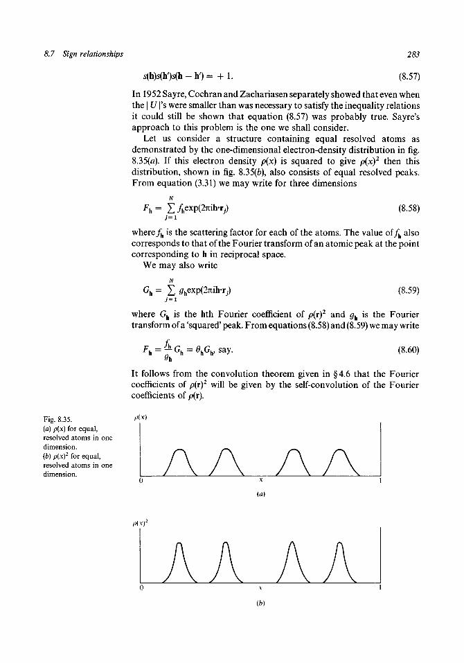
8.7 Sign relationships 283
s(h)s(h>(h - 1 0 = + 1. (8.57)
In 1952 Sayre, Cochran and Zachariasen separately showed that even whenthe | U |'s were smaller than was necessary to satisfy the inequality relationsit could still be shown that equation (8.57) was probably true. Sayre'sapproach to this problem is the one we shall consider.
Let us consider a structure containing equal resolved atoms asdemonstrated by the one-dimensional electron-density distribution in fig.8.35(a). If this electron density p(x) is squared to give p(x)2 then thisdistribution, shown in fig. 8.35(fc), also consists of equal resolved peaks.From equation (3.31) we may write for three dimensions
Fh= Z /hexP(27lih'r;) (8.58)
where/h is the scattering factor for each of the atoms. The value of/h alsocorresponds to that of the Fourier transform of an atomic peak at the pointcorresponding to h in reciprocal space.
We may also write
Gh = (8.59)
where Gh is the hth Fourier coefficient of p(r)2 and gh is the Fouriertransform of a 'squared' peak. From equations (8.58) and (8.59) we may write
say. (8.60)
It follows from the convolution theorem given in §4.6 that the Fouriercoefficients of p(r)2 will be given by the self-convolution of the Fouriercoefficients of p(r).
Fig. 8.35.(a) p(x) for equal,resolved atoms in onedimension.(b) p(x)2 for equal,resolved atoms in onedimension.
x
(a)
Pix)2
x
(b)

284 The determination of crystal structures
From equation (4.72) it can be seen that the Fourier coefficients of p(r)are (l/K)Fh and similarly the Fourier coefficients of ph(r)
2 will be (l/V)Gh.Hence, from the convolution theorem
Lr -VLF LFV
Uh~ Ly^W i/^h-h'v h
and, using equation (8.60), we find
This equation, known as Sayre's equation, applies to any equal-atomstructure whether centrosymmetrical or not. It will apply to one- ortwo-dimensional data if the atoms are resolved in the appropriate projectionand then /, the length, or A, the area, of projection will replace Kin equation(8.61).
Sayre illustrated the application of equation (8.61) with a centrosymmetricalone-dimensional model structure. This had atoms at ±0.113, ±0.234,±0.361 and ±0.438 in a cell of length 20 A. The electron density in theatoms was taken as
p(u) = e-2*»2 (8.62)
where u is the distance from the centre of the atom, and this gives ascattering factor
The squared density was
p(u)2 = Q-^u2 (8.64)
with a Fourier transform
gs = ^~^\ (8.65)
The reciprocal-lattice distance s is related to the structure-factor index h by
s = - (8.66)a
so that
y ^ V ( ^ Y (8.67)
Structure factors were calculated for the structure and the two sides ofequation (8.61) were then compared. The results are shown in table 8.8.
The agreement of the two sides of the equation is excellent; anydisagreement is due to the termination of the Fourier series and to slightoverlap of the electron density between atoms.
Sayre actually used his equation to solve a crystal structure but generallythis is not feasible. What can be seen from these equations is that if Fh is

8.7 Sign relationships 285
Table 8.8.
h
0123456789
10111213
F
5.66-1.00-0 .41-0.48-1.28
0.35-1.78-0 .54
1.412.80
-1.290.48
-0.64-0.52
5.66-1.00-0.41-0.48-1.27
0.35-1.78-0.54
1.412.79
-1.300.47
-0.62-0.52
h
14151617181920212223242526
F
0.38-1.81
0.770.720.38
-0.05-0.07-0.10-0.03-0.17-0.37
0.360.03
o , l F h F h h
a h,
0.37-1.78
0.760.720.38
-0.07-0.05-0 .10-0.03-0.16-0.36
0.350.03
large then any large products on the right-hand side of equation (8.61) arelikely to have the same sign as Fh or
s(h)s(h')s(h - h') « 1 (8.68)
where « means 'probably equals'. Cochran and Zachariasen also arrived atthis probability relationship although by different lines of reasoning.
The probability that equation (8.68) is true was worked out for theequal-atom case by Woolfson (1954). We write the unitary structure factoras the sum of independent terms
N/2uh = Z 2nicos(27ih-rJ.)
j= i
N/2
= £ 2nJcos(27ih/-ri)cos{27i(h-h/)TJ.}
N/2
- X 2nisin(27ih/TJ.)sin{27i(h - h ^
This can be written as
N/2 N/2
^h = I "j + Z Pj
where
and
pj = 2rijsin(2Txh/-r7.)sin{27i(h - h')-r,.}.
(8.69)
(8.70)
(8.71a)
(8.71b)

286 The determination of crystal structures
The central-limit theorem tells us that the probability distribution of Uh
is normal with a mean
N/2 N/2
^h = I OLJ + £ pj (8.72)
7 = 1 7 = 1
and a variance from equation (7.18)
N/2 N/2
<= I (*,2-00+ KPj-TA (8-73)7 = 1 7 = 1
Now
a,. = 2n/cos(2iih'-r/)cos{27t(h - h')* .}
= 2n/cos(27th'-r/) x cos{27i(h - h')-r,.} (8.74)
taking the product of the averages is valid since the two quantities areindependent.
When the atoms are equal rij = N'1 and
N/2 N2n/{cos 27thT/.) = 2rij x — x (cos 2jth-r/)
2
= cos(27ih-rj) = Uh. (8.75)
Hence
^ = 2N-'UWU^. (8.76)
We also have
Pj = 2n/sin(27th'T,.) x sin{27i(h - h')-r,.} = 0 (8.77)
since the values of sin(2iihTJ.) are equally probably positive and negativeand not constrained by the value of Uh - as long as | Uh | is not exceptionallylarge.
This gives, from equations (8.72) and (8.76),
N/2uh = Z 2AT1L/h>Uh_w = Uh Uh_h,. (8.78)
7 = 1
As long as Uh>Uh_h, is not too large we can write
N/2 N/2h Z—i j /-^ • j
7 = 1 7 = 1
N/2
= X 4n2 cos2(27ihr-rj) x cos2{2ii(h7 = 1
N/2
X 4n2 sin2(27ih-rJ.) x sin2{27i(h - h')-^.}. (8.79)7 = 1
If we take sin2(27ihTJ) = cos2(27ihTJ) = \ then we find for equal atoms
o2h = N-\ (8.80)

8.7 Sign relationships 287
Thus for a particular pair of unitary structure factors Uw and Uh_w thedistribution of the values of Uh is
= (2TCAT *) exp{ - ±N(Uh - Uh.Uh_h.)2}. (8.81)
However we know the value of | t/h | and the value of Uh is eithers(h>(h - h') | l/h | or -s(h')s(h - h') | Uh' |. The probability of it having eachof these values is proportional to the ordinate of the distribution (8.81).These two values correspond to s(h)s(h')s(h — h') being positive and negative,respectively; if we denote the probabilities by P+(h,h') and P_(h,h') then
P+(h,h) _ exp{ -±N(\Uh\ ~ 1 E W - r I ) 2 } 2Nl v v u
^UMO " exp{-| iV(|l /h | + | l / h ^ h _ J ) 2 } " CXP(2iV' U>U> U
(8.82)
Since we must have P+(h,h') + P_(h,h') = 1 we can find
P+(h,h') = i + $tznh(N\UhUh.Uk-h.\). (8.83)More accurate probability expressions, and ones which apply to
structures with non-equal atoms, have been given by Cochran andWoolfson (1955), Bertaut (1955) and Klug (1958).
In table 8.9 there are shown some typical values of P+(h, h') for N = 20,
40 and 80 and for a range of values of 0 = (| UhUh,Uh_w | )*.The probabilities given by equation (8.83) tend to be somewhat lower
than those given by the more precise theories although the expressiondoes become more accurate as N increases. The expression also givesP+(h,h')# 1 in some situations where inequalities apply. However, inpractice, one is not normally interested in the exact probabilities when oneis using expression (8.68), the triple-product sign relationship (t.p.s.r.).
These relationships were first used by Zachariasen (1952) in solving thestructure of metaboric acid. By inequality relationships he was able to findthe signs of forty structure factors in terms of five sign symbols. NextZachariasen extended the sign information and found relationships betweenthe symbols by the use of
(8.84)
where the summation was taken for all products of structure factors for
Table 8.9.
U N = 20 40 80
0.00.10.20.30.40.5
0.5000.5100.5790.7570.9280.993
0.5000.5200.6540.8960.9941.000
0.5000.5400.7820.9871.0001.000

288 The determination of crystal structures
which signs or sign symbols were known. This relationship is anapproximation to the more accurate relationship
(8.85)
which has an associated probability
) (8-86)
where P+(h) is the probability that Uh is positive. It will be noticed that if thesummation is negative then P+(h) < \.
In a typical application of equation (8.84) it might be found that theseparate products in the summation were aaaaababab. This would betaken as an indication that s(h) = a and b = 4- 1. If other indications gaveb = + 1 it could soon be accepted with some confidence.
As an example we consider the determination of signs for the c-axisprojection of Roussin's red ethyl ester (Thomas, Robertson & Cox, 1958).The structure has two molecules of (NO)4Fe2S2(C2H5)2 per unit cell andhas space group P2Ja with a = 7.81, b = 12.67, c = 7.01 A and /? =111°24/. The c-axis projection has the two-dimensional space group pggand the table of | U |'s is shown in fig. 8.36.
We should note that, for this space group, equivalent reflections inneighbouring quadrants have signs related by
s(h,k) = (- l)h+ks(h,k). (8.87)
The two origin-fixing reflections are chosen by taking
S(7,3) = 5(5,8)= + 1 .
The first few stages of sign determination by inequalities give:
h h' h + h' h - h' Conclusion
^7,3 ^5,8 IUl2.nl 1^2.3 I 5 ( 2 , 5 ) ^ - 5 ( 2 , 5 )= 0.78 = 0.58 = ? = 0.24 = + 1
U 7 f l l / 7.i | f / 1 4 t 0 l I U0.21 *(0,2) = + 1= 0.74a = 0.14a =1 =0.26
U7,3 U0,2 | I / 7 f 5 | l/7fl 5(7,5) = + 1= 0.78 = 0.26 = 0.57 = 0.74a and a = + 1
U5,8 | l / 2 i 3 | t/7,5 | l / 3 f l l | 5(2,3) = -5 (2 ,3 )= 0.58 = 0.27 = 0.57 = 0 = 4 - 1
Inequalities can be applied, with the introduction of more sign symbols,until virtually all the larger l/'s have their signs determined. In fig. 8.36 thereis shown a stage where 23 signs are determined in terms of four symbols.One can easily go further and find explicitly what all the symbols representbut the process has been stopped here to demonstrate the application of thet.p.s.r.
All the signs and symbols in fig. 8.36 should be marked on a transparent
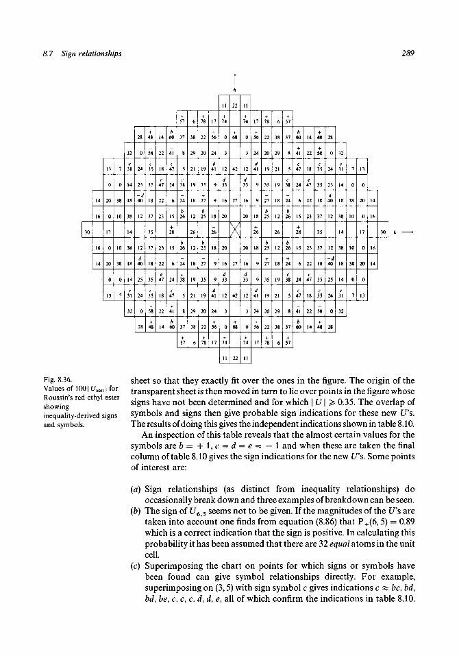
8.7 Sign relationships 289
30
14
16
16
14
13
0
20
0
17
0
20
0
13
7
0
38
10
10
38
0
7
32
e31
14
18
38
14
38
18
14
e •31
32
28
0
24
25
-d40
12
12
d40
25
24
0
28
48
58
35
35
18
37
35
37
18
35
35
+58
+48
14
22
18
e47
22
23
23
22
e47
18
22
14
b60
41
c47
24
6
15
+28
15
6
24
c47
+41
b60
57
37
8
5
38
+24
b26
b26
_24
c38
5
8
37
+57
6
38
29
21
19
18
12
26
12
18
19
21
29
38
6
78
22
20
19
35
+27
b25
b25
_27
35
19
20
22
+78
17
-f56
24
d41
9
9
18
+26
18
9
9
d41
24
+56
17
11
74
0
3
12
d33
16
20
20
16
d33
12
3
0
+74
11
22
+68
42
27
X27
42
+68
22
11
74
0
3
12
d33
16
20
20
16
d33
12
3
0
+74
11
17
+56
24
d41
9
9
18
+26
18
9
9
d41
24
56
17
78
22
20
19
35
_
27
b25
b25
+27
35
19
20
22
+78
6
38
29
21
19
18
12
26
12
18
19
21
29
38
6
57
37
8
5
c38
_
24
b26
b26
+24
c38
5
8
37
+57
b60
+41
c47
24
6
15
+28
15
6
24
c47
41
b60
14
22
18
e47
22
23
23
22
e47
18
22
14
+48
+58
c35
35
18
37
35
37
18
35
c35
58
+48
28
0
24
25
d40
12
12
-d40
25
24
0
28
32
e31
14
18
38
14
38
18
14
e31
32
7
0
38
10
10
38
0
7
13
0
20
0
17
0
20
0
14
16
16
14
30
Fig- 8.36. sheet so that they exactly fit over the ones in the figure. The origin of theValues of 1001 Uhk01 for transparent sheet is then moved in turn to lie over points in the figure whoseRoussin's red ethyl ester signs have not been determined and for which | U | ^ 0.35. The overlap ofshowinginequality-derived signs symbols and signs then give probable sign indications for these new U's.and symbols. The results of doing this gives the independent indications shown in table 8.10.
An inspection of this table reveals that the almost certain values for thesymbols are b = + 1 , c = d = e = — 1 and when these are taken the finalcolumn of table 8.10 gives the sign indications for the new (7's. Some pointsof interest are:
(a) Sign relationships (as distinct from inequality relationships) dooccasionally break down and three examples of breakdown can be seen.
(b) The sign of U6t5 seems not to be given. If the magnitudes of the l/'s aretaken into account one finds from equation (8.86) that P+(6,5) = 0.89which is a correct indication that the sign is positive. In calculating thisprobability it has been assumed that there are 32 equal atoms in the unitcell.
(c) Superimposing the chart on points for which signs or symbols havebeen found can give symbol relationships directly. For example,superimposing on (3,5) with sign symbol c gives indications c « be, bd,bd, be, c, c, c, d, d, e, all of which confirm the indications in table 8.10.
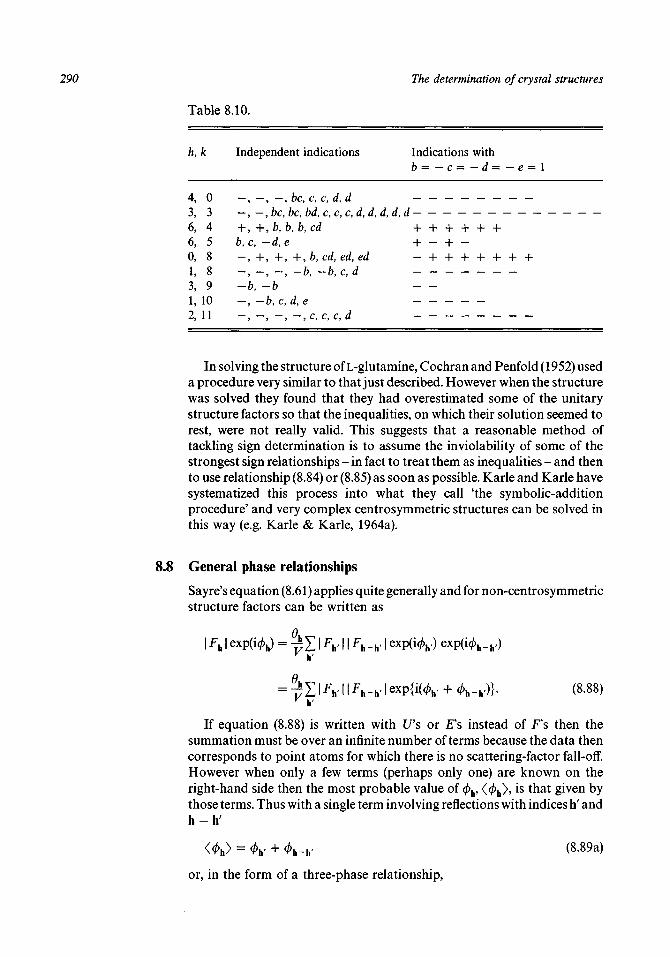
290 The determination of crystal structures
Table 8.10.
h, k Independent indications Indications withb = — c = — d — — e — \
4, 0 - , - , - , be, c, c, d, d3, 3 - , - , be, be, bd,c,c,c,d,d,d,d,d •
6,6,0,1,3,1,2,
45889
1011
+ ,+,b,bb, c, —d,e— + +_ 9 —9 — 9
-b, -b '
—, —b,c,(_ _ _ _ _ _
,b,cd
+ ,b,cd,
-b, -b,
d,e—, c, c, c
edc,
,d
edd
+ + + + + ++ - + -_ _ j _ _l_ _l_ _l_ _l__ _ _ _ _ _ _ _ _
— —_ _ _ _ __ _ _ _ _ _
In solving the structure of L-glutamine, Cochran and Penfold (1952) useda procedure very similar to that just described. However when the structurewas solved they found that they had overestimated some of the unitarystructure factors so that the inequalities, on which their solution seemed torest, were not really valid. This suggests that a reasonable method oftackling sign determination is to assume the inviolability of some of thestrongest sign relationships - in fact to treat them as inequalities - and thento use relationship (8.84) or (8.85) as soon as possible. Karle and Karle havesystematized this process into what they call 'the symbolic-additionprocedure' and very complex centrosymmetric structures can be solved inthis way (e.g. Karle & Karle, 1964a).
8.8 General phase relationships
Sayre's equation (8.61) applies quite generally and for non-centrosymmetricstructure factors can be written as
I *h I exp(i0h) = ^Y | Fh. 11 Fh_h, | exp(i</>h,) exp(i</>h_h,)
+ </>h-h')}- (8-88)v h'
If equation (8.88) is written with IPs or £'s instead of F s then thesummation must be over an infinite number of terms because the data thencorresponds to point atoms for which there is no scattering-factor fall-off.However when only a few terms (perhaps only one) are known on theright-hand side then the most probable value of 0h, <</>h>, is that given bythose terms. Thus with a single term involving reflections with indices h' andh-h'
<A> = K + h-w (8-89a)or, in the form of a three-phase relationship,

8.8 General phase relationships 291
h ~ <t>h'- <t>h-h' ~ ° (modulo 2n) (8.89b)
which means that the combination of three phases has a distribution about0 or some multiple of 2n.
If there are a number of pairs of phases which, on the right-hand side ofequation (8.89a), all contribute to an estimate of </>h then the probable valueof tan 0h may be found from
<tan 0h> = ± . (8.90a)
Equation (8.90a) with £'s (see equation (7.44)) instead of U's was first givenby Karle and Hauptman (1956). This equation is referred to as the tangentformula and it has played a very important role in the development of directmethods of solving crystal structures. Another form of the tangent formula,which has a better theoretical basis, is
</>h_h,)<tan 0h> = X = h
where
*(h,h) = 2AT*|£h£h,£h_h,|. (8.90c)
If the atoms in the structure are not all equal then N, the number of atoms inthe unit cell, is replaced by a more complicated expression but normally itsvalue will not be very different from N.
The actual value of 0h will in general be different from the most probablevalue given by equation (8.89a) but the larger the value of ?c(h, h') for thatrelationship the smaller the difference one is likely to get. The general formof the probability distribution of c/>h has been given by Cochran (1955) and isshown in fig. 8.37. It is of the form
P ( I <t> - l/ 0 is the modified Bessel function which also appears in equation (8.17). Thelarger is jc(h, h') the smaller is the variance of the distribution and the morelikely it is that the estimated value from equation (8.89) will be close to thetrue value. If equation (8.90) is used to estimate 0h then the same probabilityrelationship is valid except that jc(h, h') is replaced by ah where
h = T\ + B\. (8.92)
Karle and Karle (1964b) solved the structure of L-arginine dihydrate, thefirst non-centrosymmetric structure to be solved by direct methods. Theyused what they called the symbolic addition method in which unknownphases are represented by letter symbols, much as was done for signs in the
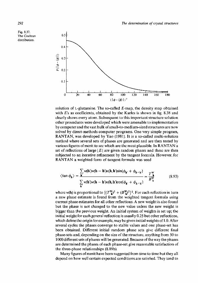
292 The determination of crystal structures
Fig. 8.37.The Cochrandistribution.
0.5 -
0.4
0.3
cu 0.2
0.1
1 i20 40 60 80 100 120 140 160 180
solution of L-glutamine. The so-called £-map, the density map obtainedwith £'s as coefficients, obtained by the Karles is shown in fig. 8.38 andclearly shows every atom. Subsequent to this important structure solutionother procedures were developed which were amenable to implementationby computer and the vast bulk of small-to-medium-sized structures are nowsolved by direct-methods computer programs. One very simple program,RANTAN, was developed by Yao (1981). It is a so-called multi-solutionmethod where several sets of phases are generated and are then tested byvarious figures of merit to see which are the most plausible. In RANTAN aset of reflections of large | E | are given random phases and these are thensubjected to an iterative refinement by the tangent formula. However, forRANTAN a weighted form of tangent formula was used
<tan0h>=Jil- h>(h,h')sin(0h,
= ^ (8-93)
-h>(h,h')cos(</>h. + <Ah_h.)
where w(h) is proportional to {(7^)2 + (B™h)2}*. For each reflection in turn
a new phase estimate is found from the weighted tangent formula usingcurrent phase estimates for all other reflections. A new weight is also foundbut the phase is not changed to the new value unless the new weight isbigger than the previous weight. An initial system of weights is set up; theinitial weight for each general reflection is usually 0.25 but other reflections,which define the origin for example, may be given initial weights of 1.0. Afterseveral cycles the phases converge to stable values and one phase-set hasbeen obtained. Different initial random phase sets give different finalphase-sets and, depending on the size of the structure, anything from 50 to1000 different sets of phases will be generated. Because of the way the phasesare determined the phases of each phase-set give reasonable satisfaction ofthe three-phase relationships (8.89b).
Many figures of merit have been suggested from time to time but they alldepend on how well certain expected conditions are satisfied. They tend to

8.8 General phase relationships 293
Fig. 8.38.The a-axis projection ofa three-dimensionalelectron-density map forL-arginine dihydrate with400 phases determinedby phase relationships(from Karle & Karle,1964b).
O(2)
N(5)
A N
C(4) \J^-
H2O(2)o
C(7)
(a)
N(9)
CIS) /
H2O(1)
N(12)
#
4^010)
Nil 1)
be rather complicated but a very simple figure of merit, not now used, is
(8.94)
where the h's are for all large | Eh | and all large | E |'s are used in evaluatingthe a's - which is just a measure of how well the three-phase relationshipsare satisfied. Another simple figure of merit is
Z = 2 > k (8.95)k
where, in this case, the values of | Ek | are small but the large | E |'s go into thesummations which give the a's. This figure of merit can best be understoodin terms of Sayre's equation (8.61) which can also be written in terms of £'s.The values of a are just proportional to the magnitude of the right-hand sideof equation (8.61) so this figure of merit is simply saying that if | E | is smallfor normal density then it is expected to be small for squared density.
We can illustrate the application of direct methods with MINDIR(appendix XI), a simple two-dimensional form of RANTAN which can beapplied to structures with any two-dimensional space group. From Sayre'sequation it is evident that the phase obtained from equation (8.93) is justthat from squaring the density of a map with coefficients w(h)£(h). The stepsin MINDIR are:
(1) A file is read in giving h, k and | E(h, k) | values in a form given by theoutput of FTOUE.
(2) A subset of large | E |'s is found for which | E \ > 1.0.(3) Random phases are generated for the subset of reflections and weights
of 0.25 are allocated.(4) A map is calculated with magnitudes of coefficients w(h) | £(h) | and
current phase estimates.

294 The determination of crystal structures
(5) The map is squared and Fourier-transformed to give Fourier coefficientsG(h).
(6) For each reflection a new weight is calculated. If this is greater than theprevious weight then the new phase and weight are accepted.
(7) If there have been less than 16 cycles of refinement or if the meanchange in phase is greater than 2° then go back to (4). Otherwise go onto (8).
(8) A final cycle of calculating a map, squaring and Fourier-transformingthe map is carried out and the final weights and phases are acceptedunconditionally.
(9) Return to (3) and repeat until a chosen number of phase-sets has beengenerated.
(10) For each phase-set calculate A, as given by equation (8.94), for all| E |'s > 1.3 and Z, as given by equation (8.95), for all | E |'s < 0.5. Thesefigures of merit are scaled to have a maximum value of 1000 andoutput for each phase-set. Also output is a combined figure of merit,CFOM, defined as
CFOM = AA ~ i4|"in + Z™* ~ Z . (8.96)
A A / /max mm max min
The subscripts refer to the maximum and minimum values of A and Zfor all the phase-sets generated and CFOM would have a value of 2.0 ifit had the greatest value of A and the least value of Z and a value of zeroif it had the least value of A and the greatest value of Z.
(11) MINDIR automatically outputs the map for the largest value ofCFOM. If this does not reveal the structure then MINDIR can be runagain using a switch which simply finds any other designated phase-setfrom a file and then computes and outputs the map without re-runningthe complete program.
Structure factors were calculated with STRUCFAC for the artificialstructure, with space group pg, shown earlier in fig. 8.17 and the output filefrom this was used with FTOUE to give a set of | E |'s. This was used as inputfor MINDIR which generated 50 phase-sets and gave the list of figures ofmerit shown in table 8.11. Solution 17 had the highest value of CFOM,1.330, followed by solution 43 with a value 1.321. The program automaticallyproduced a map for solution 17 which is shown in fig. 8.39. The followingpoints will be noted. The sodium atoms appear clearly but overweightcompared with other peaks in the map. This is a common feature ofsolutions produced with the tangent formula because, as we have seen withMINDIR, the application of the tangent formula is tantamount to squaringthe electron-density, which tends to increase density differences and makesheavier atoms appear stronger than they should be. The correct positions ofthe light atoms all fall on positive density although two do not fall withincontoured regions; in addition there is a considerable amount of spuriousdensity. All these features are seen in the results from the large andcomplicated direct-methods computer packages which are commonly used,but to a lesser extent. Finding new phases in series, one at a time, by thetangent formula, rather than by squaring the map and producing large

8.8 General phase relationships
Table 8.11. Figures of merit from MINDIRfor the structure C3H5N2ONa2
295
The values of A and Z are as given in equations (8.94) and (8.95). Solution 17 has the highest combinedfigure of merit, CFOM.
THE SEED USEDSOLN
13579
1113151719212325272931333537394143454749
A997.3970.2963.7488.91000.0258.6983.7889.4628.0980.7399.9263.8707.6998.5996.1928.6996.2734.0426.8404.7950.2705.8925.7499.4952.6
IS 9000Z948.1872.8889.4369.91000.0152.6942.1656.2314.1940.8264.4238.9426.7941.0984.1761.7985.3725.5400.9257.2854.0399.6785.3349.8847.0
CFOM1.0511.1021.0781.1281.0001.1161.0431.2441.3301.0421.1451.0311.2951.0601.0131.1751.0111.0111.0311.1581.1011.3211.1471.1591.111
SOLN2468
101214161820222426283032343638404244464850
A311.035.3
925.0300.5991.4926.5991.2516.0766.5996.0988.2990.9239.5404.6264.541.480.1
555.3243.6408.7986.4730.3931.0851.7277.3
Z198.341.5
817.3177.5971.7716.8964.7336.2517.3972.5955.9966.5112.9152.5268.744 .764.0
410.1136.4285.6928.6479.9796.9648.5339.3
CFOM1.1221.0001.1131.1331.0211.2191.0281.1911.2621.0251.0341.0251.1371.2671.0011.0031.0231.1551.1171.1321.0601.2631.1401.2130.940
numbers of new phases in parallel, dampens the squaring effect. Again, inthree dimensions the ratio of the number of data employed to the number ofatomic positions to be determined is much greater than in two dimensionsand gives better resolution of the structure; it should be noted that 400reflections in three dimensions have gone into the £-map given in fig. 8.38.Nevertheless the general principles of direct methods are well illustrated byMINDIR.
A characteristic of direct methods when applied to non-centrosymmetricstructures, as with almost all other methods, is that the structure obtainedmay be the true structure or its enantiomorph. If, for example, thepositions of all atoms are changed from (x, y) to (x, y) then the magnitudesof the structure factors are unchanged. For that reason, when solving anunknown non-centrosymmetric crystal structure when only the experimental| F |'s are available, either form could be found by the structure-solvingmethod. Organic molecules very often occur in either a right-handed orleft-handed form represented by the prefixes D (dextro) or L (laevo). Thetwo forms are related to each other as a left hand is to a right hand and twomolecular structures of different chirality may be arranged so as to be

296 The determination of crystal structures
Fig. 8.39.The direct-methodssolution ofC3H5N2ONa2 from theprogram MINDIR.(Solution 17 from table8.11 with ,4 = 628.0,Z = 314.1 andCFOM = 1.330.)
SOLUTION NUMBER 17 A, Z, CFOM =OUTPUT WITH Y HORIZONTAL AND ORIGIN
628.0 314.1 1 . 330TOP LEFT
10 11 12 13 14 15 16 17
0
1
2
3
4
5
6
7
8
9
10
1 1
12
13
14
15
16
17
18
19
20
21
22
23
24
25
26
27
28
29
30
31
32
- 3 2
-13
7
- 2 0
- 2 7
0
1 5
2 1
24
7'
- 9
- 5
- 7
- 1 2
- 6
- 5
- 7
1
- 2
- 7
10
19
2
- 1 1
- 1 5
- 1 8
- 3
9
- 6
4
32
7
-32
- 1 1
14
27
6
- 3
2
- 2
vN
14
5
- 1 3
- 1 1
4
- 1 2
- 2 8
- 2
14
- 2
- 3
8
4
3
10
1 1
2 3
( 3 3
s
-11
-3
-6
- 1 1
- q
;-23V. ^ 2 8 ^ - 8
. 10
. 3
. 0
. -5
. 2
7
! i
. 7
. 10
.-10
.-10
. 5
.-20
.-42
. -9
. 10
.-20
.-26
-3
. 5
1 1
22
. 13
N
. 27
>. 17
. - 1 6
-29
. - 2 1
-7,
. -15
. -9
1
. 12
• 2J
i ?
. -3
7
. 8
. 9
. 3
. -3
?> 5
. 1 8 W 4
. -5
. 2
. 11
. -12
. -13
. 15
. -1
. -27
. -5
. 8
. -14
. -5
. 20
7
. -4
. 7
. -3
. -18
•1 0
' ' 16
. 6
. -5
. -9
. -1
. 18r
• 2 l
. -2
. 9
. 2
. -3
. 2
. -4
. 3
. 6
. -1
. 6
. 12
. 1
. -5
. -6
. -7
~ 3 -
. - 1 4 .
.^22 ,
. - 1 9 .
. - 1 2 .
. - 8 .
v 2 0 - 2 1-
V 3 9
. "V
. -6
.a?.
. 3 .
. 2 3 ^ 1 3 .
. 30
. 5
. -7
.-10
.-13
. -8
. -8
^ 1 1 .
. - 1 .
. - 3 .
. - 9 .
. - 9 .
. 3 .
. 4 .
i ?
c- 1 1 S
- 1 5 .
6 .
5 .
- 2 .
2 .
- 1 .
- 8 .
- 2 0 .
- 2 9 .
~~ c^ 5
- 1
2
- 1 3
- 2 3
- 6
4
2
2
- 4
) 5
-IS.
- 1 4 .
0 .
- 5 .
0 .
A3 .' 7 .
- 3 .
- 1 6 .
- 3 1 .
-10.^
f-X
4 .
1.
2 .
- 1 4
- 4
4
- 1 0
- 2 0
-23
-17
1
2
- 8
. 2 4
fsOV 3 3
-16
-28
- 1 8
. -1
. 16
. 8
. -7
. -1
. -6
. -13
. -3
. 2
. 6
. 13
. 2
. -15
. -24
. -15
. 2
. -2
. - 1 1
2
7
. -4
N
* *32
r ' l 4
. 4
. 17
. 7
26
Na
.-19
. 11
. 12
. -1
. -2
.-12
.-18
. -5
. -4
. 13
. 5
.-16
- 2 7
.-10
. 17
. 12
.-12
. -9
. 1
. -5
. -3
•1 " 3
' - 1 4
. 9
32
. 7 .
V 32".
*v 4 •
. 9.
. - 3 .
. - 18 .
. - 1 5 .
. - 1 1 .
. 2.
. 19T
. -7 .
. - 2 .
. 1.
. -7 .
. - 5 .
. - 6 .
. - 12 .
. - 7 .
. - 5 .
. - 9 .
7 .
- 6 .
) " 3 .
- 1 1 .
vio.
X 2 3 <
1 1 .
1 0 .
3 /
- 3 .
- 2 .
1 4 .
- 2 .
- 2 8 .
- 1 2 .
4 .
- 1 1 .
- 1 3 .
5 .
1 4 .
, 2 0 ,r \
. 24 ( 19/.
• 2L. 15 .
. 0.
. - 2 7 .
. - 2 0 .
; 1
r-'i3.
A.-2.
2.
- 3 .
6 .
{
14 >
3
- 2 1 .
- 2 9 .
- 1 6 .
J7
122.
1 1 .
5 .
- 3 .
- 2 6 .
- 2 0 . -
1 0 .
- 9 .
- 4 2 . -
- 2 0 .
5 .
- 1 0 . -
- 1 0 . -
10.
7 .
1 .
7 .
2 .
- 5 .
0 .
3 .
1 0 . -
-9
-5
6
16
—er
1 8
- 3
7
- 4
7
20
- 5
14
8
- 5
27
- 1
1 5
13
12
11
2
- 5
1 8
t27
\12
1
- 9
15
-8
- 5
. -8
. -8
. -13
. -10
. 5
• Y• i\. -6
. 9
.' 39i\^—
. -4
. 2
. - 3 .
. 2 .
• t}\'3
4
3
- 9
- 9
- 3
- 1
V1
' 1 3
3
^ 2 2
(7Z
- 8
- 1 2
- 1 9
. "NaT
. - 2 .
. 18\
. - 1 .
. 4 .
) 5
. - 3 .
. 3 .
. 9.
. 8.
. 7 .
. - 3 .
- 1 4
1 °^ 3
- 7
- 6
- 5
1
12
6
-1
6
3
1 ?
. 2 .
1 .
. 4 .
^ 2 ^
.-id\
. - 3 1 .
. -16.
. - 3 .
^ \ 7 "
. /o.
/ l 4 .
(.-16.
y4l)
. - 2 9 .
. - 2 0 .
. - 8 .
. - 1 .
. 2 .
. - 2 .
. 5 .
. 6.
. - 1 5 .
. - 1 1 .
}ij
- 1 8 .
- 2 8 .
c
if.- 8 .
2 .
1.
- 1 7 .
^ 3 .
- 1 0 .
4 .
-4 .
- 1 4 .
\ ~ 2 '
' 5 .
- 5 .
-4 .
2 .
2 .
4 .
- 6 .
- 2 3 .
- 1 3 .
2 .
- 1 .
w
7
17
4
JL4
- 4
7
2
- 1 1
2
- 1 5
- 2 4
- 1 5
2
13
6
- 3
2
-3
-13
- 6
- 1
- 7
8
16
- 1
" 2 0
I
. 12.
. "9.
. -14 .
\.1 - 3 ./
\ " 3
. 1.
. -9
. -1Z.
. 1 2 .
. 17.
. -10 .
. - 2 7 .
. - 16 .
. 5.
. 13.
. -4 .
. -16 .
. - 6 .
. - 5 .
. - 1 8 .
. - 12 .
. - 2 .
. - 1 .
. 12.
. 11 .
. - 1 9 .
x - 1 3 .
-13
j 7
- 2 0
- 2 7
0
15
2 \
7
- 5
- 7
- 1 2
- 6
- 5
- 7
1
- 2
- 7
10
19
2
- 1 1
- 1 5
- 1 8
- 3
9
- 6
4
32
7
related by either a centre of symmetry or a mirror plane. In fig. 8.40 twoenantiomorphic structures are illustrated; in this case the molecules in thetwo enantiomorphs are related by a mirror plane. The solution shown infig. 8.39 has a change both of origin and enantiomorph compared to thestructure shown in fig. 8.17.
The exception to the rule that either enantiomorph may be found in thestructure solution is when anomalous scattering is used. If for oneenantiomorph | F(h) | > | F(h) | then for the other | F(h) | < | F(h) | and so thesolution may be found for the correct form of the crystal.

8.9 A general survey of methods
Fig. 8.40.An illustration ofenantiomorphicstructures in twodimensions.
297
8.9 A general survey of methods
The range of methods available to the crystallographer represents aformidable armoury, even for tackling structures of very great complexity.The examples given in this chapter have tended to be organic, orpseudo-organic, structures. This is partly because the majority of structuressolved are of this type and also because, as molecular structures, they areclearer for demonstration purposes. On the other hand, metallic alloys andminerals are often three-dimensional framework-like structures and frequentlythey involve arrangements of atoms in special positions.
The methods which have had the greatest impact on structuralcrystallography are the heavy-atom method and that of isomorphousreplacement which, applied to proteins and other macromolecular structures,have led to tremendous advances in the subjects of biochemistry andbiophysics. However the widescale availability of synchrotron radiation ischanging the pattern in macromolecular crystallography so that the use ofanomalous scattering should increase, perhaps to the point where it maybecome the method of choice. Many native proteins contain atoms suitablefor anomalous-scattering experiments, for example, iron, calcium or evensulphur, and anomalous differences can be relied upon to the resolutionlimits of the data - unlike isomorphous replacement where the addition of aheavy-atom-containing group somewhat distorts the structure so thatisomorphism breaks down at higher resolutions.
For most small-to-medium structures - up to 150 or so non-hydrogenatoms in the asymmetric unit - direct methods are usually used becausethey are so automatic. Indeed, where high resolution (~ 1 A) data of goodquality are available it has been shown that small proteins with up to 500 orso atoms in the asymmetric unit can also be solved by direct methods. Theoldest of the systematic approaches, the Patterson method, still has an

298 The determination of crystal structures
important role to play, for example it can be used to locate heavy atoms asthe first stage of solving a complex structure. There are also available verypowerful image-seeking Patterson methods which often succeed whendirect methods have failed, as sometimes they do.
Problems to Chapter 8
8.1 The c-axis Patterson projection of the structure of cuprous chlorideazo-methane complex (Cu2Cl2C2H2N2) is shown in fig. 8.41. The spacegroup is P\ with one molecule per unit cell. Solve the crystal structureas completely as possible.
8.2 A two-dimensional structure of space group p2, with a = 10, b = 5 Aand y = 98° has the following content of one asymmetric unit:S (0.150,0.300), C (0.175,0.600), C (0.075,0.750),C (0.375,0.350), C (0.325,0.600), C (0.350,0.850).(i) Calculate structure factors with STRUCF AC for X-ray wavelength
k = 1.542 A and temperature factor B = 2.0 A ~2.(ii) Calculate a Patterson function with FOUR2 and find the position
of the S atom.(iii) Calculate the contribution of the S atoms with STRUCFAC.(iv) Use the program HEAVY to produce a data file, SF.DAT with the
phases given by S and structure amplitudes with centrosymmetricheavy-atom weights,
(v) Calculate a Fourier synthesis with program FOUR2 and data fileSF.DAT to find the remaining atoms.
8.3 A structure which is isomorphous with that described in Problem 8.2has sulphur replaced by oxygen.(i) Calculate structure factors for this crystal, again for X = 1.542 A
and temperature factor B = 2.0 A"2, putting the result in data fileSF2.DAT.
(ii) Run program ISOFILE to give coefficients for a differencePatterson in an output file SF.DAT.
(iii) Run FOUR2 with SF.DAT to give a difference Patterson andlocate the i-r atom.
8.4 A two-dimensional structure, space group pi with a = 8, b = 5 A andy = 95°, has atoms with the following coordinates:S (0.563,0.300), S (0.375,0.200), S (0.125,0.600),C (0.313,0.500), C (0.469,0.750), C (0.656,0.650),C (0.813,0.800), C (0.875,0.500).An isomorphous compound exists with oxygen replacing sulphur,
(i) Calculate the structure factors for the sulphur compound forX = 1.542 A with temperature factor B = 2.0 A" 2 using STRUC-FAC and place the results in file SF1.DAT.
(ii) Similarly calculate structure factors for the oxygen compoundand place in file SF2.DAT.
(iii) Use ISOFILE to find the coefficients of the difference Pattersonand place them in data file SF.DAT.
(iv) Use FOUR2 to calculate the difference Patterson. Confirm that

Problems to Chapter 8 299
Fig. 8.41.The c-axis Pattersonprojection ofCu2Cl2C2H2N2 (seeProblem 8.1).
0 0.1 0.2 0.3 0.4 0.5 0.6 0.7 0.8 0.9 0
\ \ \ \ \ \ \ \ \ \ \0 0.1 0.2 0.3 0.4 0.5 0.6 0.7 0.8 0.9 0
this can be interpreted as vectors from the three i-r atoms,(v) Calculate structure factors for the sulphur atoms alone and place
in data file SFIRA.DAT.(vi) Calculate structure factors for the oxygen atoms alone and place
in data file SFIRB.DAT.(vii) Use the program ISOCOEFF with the data files SF1.DAT,
SF2.DAT, SFIRA.DAT and SFIRB.DAT to generate the Fouriercoefficients of a map which should show the carbon atoms,
(viii) Use FOUR2 with the output file from ISOCOEFF and find thecarbon positions.
1.5 Data is taken for the structure described in Problem 8.4 with themodification that the second sulphur atom is replaced by carbon. FeKax radiation (2. = 1.936 A) is used giving anomalous scattering fromthe remaining two sulphur atoms with/x = 0.385 and/2 = 0.846.(i) Calculate structure factors with STRUCFAC including the
anomalous contributions from sulphur,(ii) Use the data file from STRUCFAC as the input file to ANOFILE
to generate anomalous difference coefficients,(iii) Use the output file from ANOFILE as input to FOUR2 to
generate an anomalous-difference Patterson map.(iv) Interpret the map to show that it is consistent with the peak
between the sulphur atoms.1.6 A two-dimensional structure, space group pi with a = 9.0, b = 6.0 A
and y = 98°, has atoms with the following coordinates:Hg (0.333,0.167), 0(0.167,0.250), 0(0.500,0.292),O (0.778,0.500), N (0.472,0.833), C (0.111,0.500),C (0.500,0.500), C (0.389,0.667), C (0.639,0.625),C (0.611,0.833).(i) Calculate structure factors for k= 1.542 A using STRUCFAC

300 The determination of crystal structures
with anomalous scattering for the mercury atom for whichfx = - 5.1 and/2 = 8.9.
(ii) Use the output file from STRUCFAC as input to PSCOEFF togenerate Fourier coefficients for a Ps-function map.
(iii) With the output file of PSCOEFF as input to FOUR2 calculate aPs function and find the positions of all atoms relative to themercury position.
8.7 The a-axis projection of dicyclopentadienyldi-iron tetracarbonyl (Mills,1958) has two-dimensional space group pgg. The values of 1001 U \ arelisted in table 8.12. By the use of inequality and sign relationshipsdetermine signs for the large l/'s. (Note: for this space group
Pom = ("~ 1) Foki-)8.8 A two-dimensional structure, space group p2 with a = 9.0, b = 6.0 A
and y = 100°, has atoms with the following coordinates:0(0.389,0.792), C (0.278, 0.167), C (0.389,0.333),C (0.306,0.583), C (0.167,0.583), C (0.139,0.333).(i) Calculate structure factors with STRUCFAC.
(ii) Use FTOUE to produce a data file with £'s.(iii) Use the E data file with MINDIR to find a direct-methods solution
of the structure.
Table i
k I
2 0
4 0
6 0
8 0
10 0
12 0
12345678910111213
o :i :2 :3 :
LLLLLIII
)II)
$.12.
100| C/|
43633403316333616910446322116281418152722
k
4567891011121312345678910111213
/
22222222223333333333333
100| t/|
13326171316633021363420303120371127216210
k
012345678910111212345678910
44444444444445555555555
100| U\
4017422511285401124150171213310122003612
k
110123456789123456701234
/
56666666666777777788888
1001 £/|
1113810290260072110024133149163802800

9 Accuracy and refinement processes
9.1 The determination of unit-cell parameters
When a crystal structure is solved and refined the solution appears as a setof fractional coordinates from which can be determined bond lengths andangles, van der Waals distances, etc. However the accuracy with whichthese quantities can be determined will depend not only on the accuracy ofthe atomic coordinates but also on the accuracy of determination of theunit-cell parameters.
By the measurement of layer-line spacings or from Weissenbergphotographs one can usually measure cell edges to about 1 % and angleswith an error of about \°. The order of accuracy of cell dimension requiredto match that of coordinate determination is about one part in a thousandor perhaps a little better. This would correspond to less than 0.002 A in abond of length 1.500 A and rarely is this order of accuracy really required.
For some other purposes more accurate unit-cell parameters may berequired - for example for measurement of thermal expansion coefficientsof crystalline materials or for investigating small changes in cell parameterswith changes of composition of the material.
There has been a great deal of work in this field and it would be difficultto mention it all. What will be done is to select an example of each of themain types of method to illustrate the ranges of techniques and accuracywhich are available.
The basic idea behind all the methods is to measure the Bragg angle for anumber of reflections. This is related to the reciprocal-lattice constants asfollows. From equation (3.29) we have
6 = h2a*2 + k2b*2 + /2c*2
S =A.
+ 2hla*c* cos jS* + 2klb*c* cos a*. (9.1)
Equation (9.1) takes on special forms for the various crystal systems. Oncethe reciprocal-space quantities have been found they can be transformedinto crystal-space quantities by the relationships in table 3.1.
In a method proposed by Farquhar and Lipson (1946) a single-crystalphotograph is taken with a camera arranged as in fig. 9A(a). The collimatorpasses through a hole in the film so that reflections for 6 close to 90° arerecorded near the centre of the film - not at the edge as is usually thesituation. By oscillating an orthorhombic crystal about an a axis in such away that the centre of the oscillation range has the c axis pointing at thecollimator one will record equivalent reflections (0/c/) and (Ofe/) on the zero
301

302 Accuracy and refinement processes
Fig. 9.1.(a) The arrangement ofthe film in theFarquhar and Lipsoncamera.(b) A symmetricaloscillation diagram forthe Farquhar andLipson technique.(c) The appearance ofthe zero layer of thefilm. The collimatorpasses through thecentral hole andhigh-angle reflectionsare near the centre ofthe film.
Collimator
I II M O I I II II I
(c)
layer symmetrically disposed about the centre of the film. The indexingchart for a photograph produced in this way is shown in fig. 9A(b) and thezero layer on the straightened-out film is represented in fig. 9.1(c). The valueof 9 for a particular reflection is found by measuring the distance x betweenequivalent reflections. If the camera radius is R then it is clear from fig. 9.1 (a)that
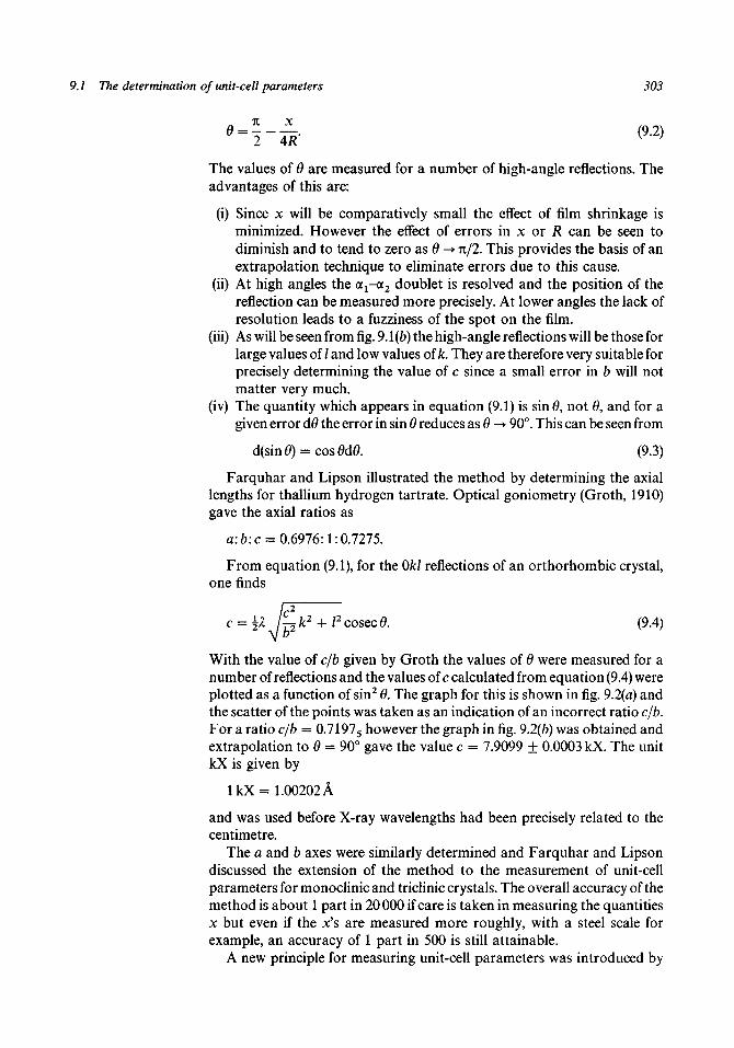
9.1 The determination of unit-cell parameters 303
The values of 9 are measured for a number of high-angle reflections. Theadvantages of this are:
(i) Since x will be comparatively small the effect of film shrinkage isminimized. However the effect of errors in x or R can be seen todiminish and to tend to zero as 9 -• n/2. This provides the basis of anextrapolation technique to eliminate errors due to this cause.
(ii) At high angles the ax-a2 doublet is resolved and the position of thereflection can be measured more precisely. At lower angles the lack ofresolution leads to a fuzziness of the spot on the film.
(iii) As will be seen from fig. 9.1(b) the high-angle reflections will be those forlarge values of / and low values of k. They are therefore very suitable forprecisely determining the value of c since a small error in b will notmatter very much.
(iv) The quantity which appears in equation (9.1) is sin 9, not 9, and for agiven error dO the error in sin 9 reduces as 9 -> 90°. This can be seen from
d(sin0) = cos0d0. (9.3)
Farquhar and Lipson illustrated the method by determining the axiallengths for thallium hydrogen tartrate. Optical goniometry (Groth, 1910)gave the axial ratios as
a:b\c = 0.6976:1:0.7275.
From equation (9.1), for the Okl reflections of an orthorhombic crystal,one finds
—k2 + /2cosec0. (9.4)
With the value of c/b given by Groth the values of 9 were measured for anumber of reflections and the values of c calculated from equation (9.4) wereplotted as a function of sin2 9. The graph for this is shown in fig. 9.2(a) andthe scatter of the points was taken as an indication of an incorrect ratio c/b.For a ratio c/b = 0.71975 however the graph in fig. 9.2(b) was obtained andextrapolation to 9 = 90° gave the value c = 7.9099 ± 0.0003 kX. The unitkX is given by
lkX = 1.00202 A
and was used before X-ray wavelengths had been precisely related to thecentimetre.
The a and b axes were similarly determined and Farquhar and Lipsondiscussed the extension of the method to the measurement of unit-cellparameters for monoclinic and triclinic crystals. The overall accuracy of themethod is about 1 part in 20 000 if care is taken in measuring the quantitiesx but even if the x's are measured more roughly, with a steel scale forexample, an accuracy of 1 part in 500 is still attainable.
A new principle for measuring unit-cell parameters was introduced by

304 Accuracy and refinement processes
Fig. 9.2.(a) A Farquhar andLipson graph for anincorrect axial ratio.(b) The improvement ofthe extrapolation whenthe axial ratio iscorrected (fromFarquhar & Lipson,1946).
X
7.92
7.91
7.90
7.89
0310o
o0210
059
CD
049
c/h = 0.7275
1
068o
o
1
* - 7.9099 kX
c/b = 0.71975
1.00 0.90
sin20
(a)
0.80 1.00 0.90
sin20
(b)
0.80
Weiss et a\. (1948). This involved the measurement of the angle between twopositions of a crystal when it gives the same reflection on opposite sides ofthe incident beam. In fig. 9.3 the normal to the reflecting planes isperpendicular to the rotation axis and, for the two positions in which thereflection occurs, the normals are along ON and ON'. It should be clearfrom the figure that the angle turned through by the crystal, NON', equals26. The technique used by Weiss et a\. was first to locate the crystal positionfor the desired reflection to within 5° by taking 5° oscillation pictures. Thecrystal was then moved by steps of \° within this range to locate the positioneven more closely and finally intensities for a fixed exposure were recordedat steps of 3' with a very finely collimated beam of X-rays to find theposition of maximum reflection. For crystals which reflect over 15' of arc,due to the finite size of the crystal and its mosaic structure, the position ofmaximum reflection could be found to within +1 ' .
By measurement of (M)0), (0/c0) and (00/) reflections the values of a*, b*and c* could be found directly. In fig. 9.4 the position of the reflecting planesis shown for the two positions of a (hOO) reflection. It should be clear fromthis figure that when the crystal is half-way between these two positions thea* axis lies along the direction of the incident beam. Thus if the crystal isbeing rotated about the c axis and (hOO) and (0/c0) reflections are recordedthen it is possible to deduce y*, the angle between the a* and fo* axes. One isthus able to measure all the reciprocal-cell parameters and thereby deducethe real-cell parameters. As used by Weiss et al. with angles measured on thegoniometer circle of the oscillation camera the method gave an accuracy ofabout one part in 104. This method was also used by Bond (1960) who useda counter to record the diffracted beam. The apparatus was accuratelymade and a finely collimated incident beam of X-rays was used. Corrections

9.1 The determination of unit-cell parameters 305
Fig. 9.3.The two reflectingpositions with normalsalong ON and ON'.
Incidentbeam
Reflected beamfor position 2
Reflected beamfor position 1
Position 2 Position 1
Fig. 9.4.Location of the a* axisfrom the two positionswhich give an (M)0)reflection.
Reflected beamposition 2
Unit cell in position 1
Unit cell in position 2
Position 1
Reflected beamposition 1
were made for the various errors that could occur and the temperature ofthe crystal was kept constant. Bond claimed an accuracy of about one partin 106. An automated instrument on similar principles has been built byBaker et al. (1966) who have measured lattice parameter changes due toradiation damage and also coefficients of thermal expansion. The accuracyclaimed is one part in 107.
A method proposed by Main and Woolfson (1963) is useful in that it usesinformation from Weissenberg photographs, which are usually availableanyway, and gives an accuracy of better than 1 part in 103. The method restson the fact that sin 6 can be determined for high-angle reflections from theseparation oia1-a2 doublets.

306 Accuracy and refinement processes
We write Bragg's law for Ka2 radiation as
sin0 = ^ (9.5)
and for the slightly different wavelength of Kax radiation
A0) = ^ - ± ^ . (9.6)
Subtracting and using the approximation sin A6 = ^A0andcos^A0 = 1we have
A0(cot 6 - |A0) = A2/1 (9.7)
For a zero-layer Weissenberg photograph
2A0 = t/r (9.8)
where t is the separation of the doublet on the film perpendicular to thecamera axis and r is the radius of the camera. From equations (9.7) and (9.8)we find
from which sin0 may be found. Although t cannot be measured veryaccurately, perhaps with an error of 3% or so for a 1 mm separation, thevalue of sin 6 is determined much more accurately. For Cu Ka radiationand a camera diameter of 57.3 mm the relationship between sin 6 and t isshown in fig. 9.5.
To determine the lattice parameters, doublet separations are measuredon zero-layer photographs so that more doublets are measured than thereare parameters to be determined. Putting s = 2 sin 6/1 and differentiatingequation (9.1) we find
sds = (h2a* + hlc* cos p* + hkb* cos y*)da*+ (k2b* + kha*cosy* + klc* cos a*)dfo*+ (l2c* + Ikb* cos a* + lha* cos jS*)dc*- /c/fc*c*sina*da* - lhc*a* sin P*dp* - Wca*fo*siny*dy*. (9.10)
Approximate values of the reciprocal-cell parameters will be known andthey can be used to evaluate the coefficients on the right-hand side. On theleft-hand side one makes s equal to the measured value and ds = s — sc
where sc is obtained from equation (9.1) by using the approximate latticeparameters. This process yields a set of linear equations in the quantitiesda*, dft*, dc*, da*, d/J* and dy*. Since there are more equations thanunknowns one can find a least-squares solution (see § 9.4). The quantitiesa* + da*, etc., are better approximations to the reciprocal-lattice para-meters and can be used for the next cycle of refinement.
The measurements on the films can be made very quickly with atravelling microscope and the parameter-refinement process is carried outby a standard computer program.

9.2 The scaling of observed data 307
Fig. 9.5.The relationshipbetween sin 6 and theseparation of the aj-areflections in aWeissenbergphotograph.
0.998
0.995
0.990
0.985
0.980
t (mm)
An extension of this technique so that measurements on higher-layerphotographs can be utilized has been given by Alcock and Sheldrick (1967).
The methods mentioned in this section are only a small selection of thoseavailable. A number of papers from a conference on The PrecisionDetermination of Lattice Parameters' at Stockholm in 1959 will be found inAda Cryst. (1960) 13, 818-50.
9.2 The scaling of observed data
The first problem of the crystallographer in collecting diffraction data is tomake sure that it is all on the same relative scale. With diffractometers, forexample, the running conditions of the X-ray tube can be strictly stabilizedand the number of counts in a given time will then be a measure of the

308 Accuracy and refinement processes
Fig. 9.6.Arranging three packs ofthree films to cover anintensity range 105:1.
intensity. By re-measuring one particular reflection from time to time onecan be sure that the scale of one's measurements is remaining steady.
Although collection of data by film methods has largely been supersededby diffractometer (§ 5.7) or image-plate methods (§ 5.9) they are still used insome laboratories and may make a comeback by the resurgence of the Lauemethod (§5.10). Normally, when collecting data on film, the diffractionspots on different films must be related to each other by empirical processes.Even if one considers a single layer of data taken with a Weissenbergcamera there are several numerical relationships to be established. Thetotal intensity range of the spots may well be 100000:1; a film whichshowed the weakest spot would be too over-exposed to measure thestrongest, which would be too dense, and a film which gave the strongestspot at a convenient intensity would not show the weakest. The greatestrange of intensity which can be comfortably measured on one film is about100:1 (two units of density). In general when a Weissenberg photograph istaken a pack of films is placed in the film holder - very often three films butoccasionally up to five. These films will differ from each other in intensitydue to the absorption of the film itself, a factor of three or so being the usualattenuation in going from one film to the one below. By comparing theintensities of spots in the conveniently measurable range one can quiteeasily deduce a film-to-film scaling factor. A scheme for taking threeseparate photographs using a pack of three films at a time is shown in fig.9.6. This will comfortably cover the range 100000:1 or even greater andprovide enough common measurable reflections in successive films to givewell-determined film-to-film ratios.
When three-dimensional data are being collected then it is necessary tomeasure the data in layers taken about two different axes. The commonreflections in intersecting layers will then provide the means of putting thedata all on the same scale.
Once the data have been put on the same relative scale then variouscorrections can be made to them - for example for spot shape (§ 5.6); the Lpfactor (§ 6.1); and absorption factor A (§ 6.2). If the measured intensity of the(hkl) reflection is denoted by Ihkl then we have
= K | (Fhkl)r |2exp( - IB sin2 0/P) (9.11)
where K is some scale factor, (Fm)r is the structure factor corresponding toscattering factors for atoms at rest and the exponential term is theDebye-Waller factor (§ 6.5). It is implicitly assumed in equation (9.11) thatthe temperature factor B is the same for each atom and is isotropic.
In order to determine the values of K and B we can make use of the resultin § 7.5 which is that
10 io2
Intensity
103 104 105 106
Film pack 1
Film pack 2
Film pack 3

9.3 Fourier refinement 309
<|J \ I 2 >= £ / ? = £. (9.12)
In equation (9.12) the structure factor has been denoted as that for atoms atrest and the scattering factors will therefore be those tabulated for rest atoms.
If we consider together a number of observed intensities all within anarrow range of sin 9 then we may write from equations (9.11) and (9.12)
</,> = K(\Fr\2}Qxp(-2Bsin2e/l2)
- IB sin2 9/X2) (9.13)
where </0> is the average of the intensities in the sin 9 range and Z0 is thevalue of Z for the particular mean value of 9. From equation (9.13) we find
Thus if the data are divided into ranges of sin 9 and ln«/0>/Z0) is plottedagainst sin2 9/X2 one should obtain a straight line whose slope is —2B andwhose intercept on one axis is In K. Such a procedure was first suggested byWilson (1942) and the graph is known as a Wilson plot.
In fig. 9.1(a) is shown a reciprocal-lattice net for the fr-axis projection ofsalicylic acid (Cochran, 1951) with intensities corrected for Lp andabsorption factors. The net shows one asymmetric unit of the reciprocal-latticelayer k = 0 and arcs of radius sin0/>l = 0.1, 0.2, etc., are drawn.
Since the space group is P2Ja the (hOl) reflections only occur for h even.The value of { J ^ ) f°r ^ e reflections which are not systematically absent istwice the average for a general reflection; this has been allowed for by takingE0 = 2Le while </#> is the average for the observable reflections. In table 9.1there are derived the values of \n((Ie}/?,'d) for four ranges of sin2 6/A2. It isassumed in this table that <sin2 9/A2} is the average for the extremities of therange and the value of T,'0 is that computed for s = 2<sin2 9/A2}*.
The values of ln«/0>/iy are plotted in fig. 9.1(b) and a straight linethrough three of the points is shown. The innermost point has been ignored;the number of reflections in the corresponding annular region is small butin any case Wilson gives reasons for not using data for low values of sin 9/X.
From the graph one finds B = 2.3 and K = 0.33. The values should beapproximately B = 4.0 and K = 0.40, and the errors from this method ofscaling are seen to be comparatively large. However, initially, one needsonly a rough scale to set about the task of structure determination. Once thestructure has been solved the observed data can be scaled to thosecalculated and the differences in the observed and calculated data then givea measure of the accuracy of the atomic parameters.
9.3 Fourier refinement
We have seen in chapter 8 that there are a large number of ways to solve acrystal structure. Basically these methods give information of one of twotypes - either a trial structure or a phase-set for the structure factors.
Let us imagine that a structure has been solved by a method that leads to
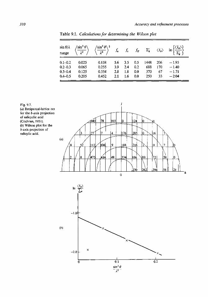
310 Accuracy and refinement processes
Table 9.1. Calculations for determining the Wilson plot
sinfl/A /sin20\ /sin20\±
\Y~ / \1T /range \Y~ / / fo fu In Ve>
0.1-0.2 0.025 0.158 5.6 3.5 0.5 1448 206 -1.950.2-0.3 0.065 0.255 3.9 2.4 0.2 688 170 -1.400.3-0.4 0.125 0.354 2.8 1.8 0.0 370 67 -1.710.4-0.5 0.205 0.452 2.1 1.6 0.0 250 33 -2.04
Fig. 9.7.(a) Reciprocal-lattice netfor the 6-axis projectionof salicyclic acid(Cochran, 1951).(b) Wilson plot for thefr-axis projection ofsalicylic acid. A
(a)
A
t
8
2/
3
52
8
/1140
/
/
27'
112
475
/
I
78
^*
1
104
414
p-—
103
4
9
49
f
0
176
188
334
124
285
216
1 6 6 \
?3C
0
0
10
262
No
\
16
\
0
72
\29^
\
\
\7\
7
\58
56
\0
A21 1
ln IT
-1.0
-2.0
0.1
sin2*
IF
0.2

9.3 Fourier refinement 311
a trial set of atomic positions - for example by an examination of aPatterson function. In order to test the plausibility of the structure onewould calculate structure factors and compare them with those deducedfrom the experimental data. To put the observed structure factors, the F0's,on an absolute scale they could be multiplied by the factor K~* deducedfrom a Wilson plot (§ 9.2) while the calculated structure factors, the Fc's,should include a temperature-factor term exp( — B sin2 6112) where B isalso given by the Wilson plot. In fact, once a trial structure has beenobtained it is customary to determine the multiplying factor which puts theobserved structure factors on an absolute scale as
where the summation is over all the structure factors for which Fc is found.The agreement between the observed and calculated structure factors is
expressed by R, the reliability index, as given in equation (8.1). Thesignificance of the value of R depends on whether or not the structure has acentre of symmetry. If observed structure factors are compared withstructure factors calculated for a structure with the correct number and typeof atoms in randomly incorrect positions the most probable values of Rwould be 0.586 for a non-centrosymmetric structure and 0.828 for acentrosymmetric structure (Wilson, 1950). We can take as a rough rule thata value of R less than 0.40 for a centrosymmetric structure or less than 0.30for a non-centrosymmetric structure would indicate a satisfactory, or atleast plausible, first trial structure.
Once an acceptable set of calculated structure factors is available a cyclicprocess of refinement can be initiated. An electron-density map is calculatedwith the magnitudes of the observed structure factors and the phases fromthe calculated structure factors, i.e.
Pr = } l I (po\ I exp{ - 2TU1IT + i</>h}. (9.16a)h
If the structure is centrosymmetric this will appear as
Pr = "pZ 5(h) I (fo\ I cos(27ih-r) (9.16b)h
where s(h) is the sign of the calculated structure factor.This electron-density map will indicate positions for the atomic centres
which will be displaced somewhat from those originally inserted and thenew atomic positions should be a better estimate of the true atomicpositions. From the new positions another set of Fc's can be calculated andthis will give a lower value of R. After a number of cycles of this process thesolution will converge and, typically, one will be left with an R somewherebetween 0.02 and 0.10 depending to some extent on the complexity of thestructure and also on the accuracy with which the data were collected. Thesituation with a centrosymmetric structure is that the refinement process isterminated when the signs of the calculated structure factors are the samefor two successive cycles; with non-centrosymmetric structure factors, onthe other hand, the phases change continuously and when to terminate the

312 Accuracy and refinement processes
refinement process is a matter of judgement. It should be stressed that foreffective refinement the problem should be greatly over-determined - that isto say, that there should be many more items of data than there areparameters to be refined.
It has been assumed above that one began with a trial structure but thesame process is valid if one starts with a trial phase-set instead. The Fouriersynthesis with the trial phases - perhaps only for some subset of the data -may give a rough but adequate picture of the structure from which a trial setof coordinates may be found and refinement initiated.
What are the underlying causes of error in this process? There will ofcourse be errors in the measurements of the Fo's but, in addition to this,there is also an error due to series termination, i.e. the limitation in theamount of data being collected. The errors in the F0's will lead to an error inthe electron density and we can estimate the extent of this.
Let pr be the calculated electron density, p'r be the electron density forerror-free data, (Fo\ the observed structure factor of index h, and F^ theerror-free structure factor. We may now write
1(9.17)
In fig. 9.8 (Fo)h and F^ are depicted on an Argand diagram. If in thecompletely refined structure the phase angles <\>^ and 0h are not verydifferent then it is clear that
where
(9.18a)
(9.18b)
Fig. 9.8.The observed structurefactor (Fo)h with theerror-free structure factorFh on an Arganddiagram.
Imaginary axis

9.3 Fourier refinement 313
Combining equations (9.17) and (9.18)
rh |exp(-27tihT + i£h). (9.19)h
From an application of the central-limit theorem (§ 7.5) we can find that theprobability distribution of Apr will be normal with a zero mean and a variance
W 2- (9.20)h
In deriving equation (9.20) the result was used that
|exp(ia)| = 1.
If the standard deviation of pT from p'x averaged over the whole cell is o(p) then
Mp)}2 = (Apr)2 (9.21)
or
a{p) = —o{F) (9.22)
where M is the total number of terms in the summation and a(F) is thestandard deviation of the errors in Fo which are assumed to be uncorrelatedwith the magnitude of Fo. When X is the wavelength of the X-radiation beingused then the explorable volume of reciprocal space is |n(2/>i)3 and, sincethe volume of a reciprocal unit cell is V~1, we find M = (32TI/3)F>1~3. Thisgives
^(p) = J—HL {2(j(F). (9.23)
Another assumption which could be made about the errors of measurementis that |AF| 2 is proportional to |F O | 2 . From this assumption one wouldhave from equations (9.20) and (9.21) that
(9.24)
where Q2 is the constant of proportionality linking | AF|2 with | Fo \2 and
P(0) is the value at the origin of the Patterson function. For atoms which arenot too heavy and for an average temperature factor one finds that
N
P(0)=^0.8 Z Zj. (9.25)
We can now make some order-of-magnitude assessment of a(p). Forexample with V = 500 A 3 , 1 = 1.54 A and a(F)=^ 1 electron we find fromequation (9.23) that <7(p)=^0.14eA~3. If the structure contains 40 carbonatoms (Z = 6) and Q = 0.10, that is to say that the average error in

314 Accuracy and refinement processes
Fig. 9.9.The shift in a peakmaximum due to thegradient of the error inelectron density.
measuring a structure factor is of the order of 10% of its magnitude, we finda(p)^ 0.15^ A"3.
The actual errors of electron density would be of interest if one waslooking for evidence of a redistribution of electron density in someparticular chemical bonding situation. However in normal circumstanceswhat one is concerned with are the atomic coordinates, and a uniformraising or lowering of the electron density in the neighbourhood of anatomic peak would not affect the precision with which this could bedetermined. What will affect the peak position will be the gradient of Ap inthe vicinity of the atomic centre. This can be seen in the one-dimensionalexample in fig. 9.9 which shows p and p + Ap in the vicinity of a maximumof p which represents the atomic position. If the maximum is displaced adistance AX from the true atomic centre, taken as the coordinate origin,then one has for a maximum of p + Ap
] = °JX=AA:
or
=0.
(9.26)
,9.27)
The slope of Ap may be assumed constant over a small range so that
In addition, from Taylor's theorem
Now the curvature of p, Cx, is given by the well-known result
c d2p/dx2
{l+(dp/dx)2p
and at the atomic centre where (dp/dx)x = 0 = 0 this gives
(9-28)
(9.29)
(9.30)
(9.31)

9.3 Fourier refinement 315
From this we find
^ 0 Go
( 9 3 2 )
The general three-dimensional result corresponding to equation (9.32)replaces differentiation by partial differentiation thus
One can find a good estimate of Co by assuming that the atomic peakchanges position but not shape so that Co is the curvature at the centre ofthe 'perfect' electron-density distribution. Hence the error in coordinate willdepend on the slope produced by the electron-density errors at the atomiccentres and one can make an assessment of the magnitude of this on astatistical basis.
If we write equation (9.19) in terms of the individual Cartesian coordinateswe have
*Px.,.z = p i l l I AFm I exp{ - 2ra(/tx + ky + Iz) + iZM} (9.34)V h k I
which gives
= G'o = p E Z E - 2™h I AF*i IexpG&H). (9.35)V h k I
The origin of the unit cell has been placed arbitrarily at the centre of theatom of interest. From equation (9.35) we can deduce that G'o should have anormal probability distribution with zero mean and with standard deviation
9-JT
G{G0) = —{Mh2fo(F) (9.36)
where o(F\ the standard deviation of the errors in the Fo's, is assumed not tobe correlated with | Fo | and M is the number of terms in the summation. Infig. 9.10 there is shown the limiting sphere with the various layers ofconstant h. A few moments study of this should convince the reader that(/i2/ max) is ^ e mean-square distance in a sphere of unit radius from adiametral plane, where /imax is the 'index' (perhaps non-integral) correspondingto sinfl = 1. This ratio may easily be found to be equal to 0.2 so that
V2 = 0.2/JLX (9.37a)
and, since /imax = 2a/A then
h? = 0 . 8 ^ . (9.37b)
Thus, with the value of M found previously, we obtain
(9.38)

316 Accuracy and refinement processes
Fig. 9.10.Layers of constant hwithin the limitingsphere.
= 3
h = 2
I
h = 2
h= - 3
where it should be noted that the units of G'o are rate of change of electrondensity per unit increase of fractional coordinate. To change this to rate ofchange of electron density per unit distance along the x direction, Go, wemust divide by the cell edge a. Hence
= 32.6 VX-(9.39)
A representation of the electron density near the centre of an atom whichis often found useful is
- p r 2 ) (9.40)
where p is typically about 4 A 2 for an atom of moderate weight with anaverage temperature factor. In equation (9.40), r is the distance from theatomic centre; the curvature at the centre can be found by differentiatingtwice with respect to r and then making r = 0. This gives
(9.41)
The standard deviation of the error of coordinate may be obtained fromequation (9.32) and is
(9.42)
(9.43a)
which, from equations (9.39) and (9.41) gives
a{AX)_iHr«W'Y.Zp \pj \VX
o(F)

9.4 Least-squares refinement 317
or, with p = 4A~2,
J (9.43b)
Thus with V= 500 A3, X = 1.54 A, Z = 6 and a(F) = 1 electron thenA
It can be shown that for a projection of area 91 the standard deviation ofa coordinate error is
2n2 , .v , .— G(F) (9.44)Z
where the two-dimensional electron density is given by
The effect of series termination is rather less easy to deal with. Effectively,it is as though the scattering factors for the atoms sharply terminate at5 = 2/A and this means that the computed electron density for an atom,instead of smoothly decreasing with increasing distance from the atomiccentre, will have diffraction ripples. These will be particularly disturbinground a heavy or even moderately heavy atom (sulphur for example) andthe error induced in the coordinates of a neighbouring atom can be greaterthan that due to errors in measurement of the | Fo |'s.
9.4 Least-squares refinement
Let us imagine for now that we have an error-free set of | Fo |'s and an almostcorrect set of atomic coordinates and temperature factors. For simplicity ofour discussion we shall assume that the structure is centrosymmetric andthe temperature factors are isotropic. The calculated structure factors willbe given by
N/2 / s :n2 gx(FXki = I 2/)exp I - Bj-jf-J cos{2n(hxj + ky, + Iz.)}. (9.45)
The correct parameters for the ; th atom can be expressed as
(Bj + ABp xj + Ax,, yj + Ayp zj + Azj)
and hence we can write
N/2 f sin2 01
= I 2/Jexpj - (Bj + A^-^ jcos^ lMx; + Ax,) + k(yj + Ayj)
+ l(zj + Azj)}l (9.46)
As long as the errors in the parameters are small this enables us to write
(F0\u ~ (Fe)m = AFhkl (9.47)
and

318 Accuracy and refinement processes
(9.48)
An equation of type (9.48) can be produced for each reflection and, ingeneral, there will be many more equations than parameters. Thus for spacegroup PT with 40 atoms in the unit cell and hence 160 parameters therecould be 2000 or more independent reflections.
The equations are linear in the corrections to be made to the parametersand, ideally, if a subset of these equations was taken such that the number ofequations equalled the number of parameters then the correct parameterscould be found and recalculated values of the Fc's would then equal the F0's.However in practice the |F J ' s are not error-free, and so one finds aleast-squares solution of the complete set of equations (9.48). This solutionis the one such that when the parameters are changed to Bj + ABp Xj + Axp
etc., the quantity
h ( ^ ) h } 2 (9-49)h
is a minimum, where (F'c\ is the revised calculated structure factor. FromTaylor's theorem we find, ignoring second-order small quantities, that
N/2
and hence
(F„)„ - (F'X = AFh - "£ (J^ABJ + ...). (9.51)
Hence Rs is the sum for all the equations of the squares of the differencesbetween the left-hand sides and right-hand sides of equations (9.48) whenthe solution is inserted and it is the minimization of this quantity which isusually implied by the term 'least-squares solution'.
It is possible to weight the equations according to the expected reliabilityof the quantity AF. If the measured | Fo | is expected to have a large randomerror then the value of AF may well be dominated by this and the AF maynot be very useful in indicating the changes to be made in the atomicparameters. Errors of measurement tend to be related to the actual value of| Fo | and many weighting schemes have been proposed based on the valueof | Fo |. One such scheme proposed by Hughes (1941) takes co = constantfor | Fo | < Fl im and co oc 1/| Fo |
2 for \FO\> Flim where Flim is some chosenupper limit of | F J for a constant weight. Another weighting schemesuggested by Cruickshank et al. (1961) is co = (a + | Fo | + c\ Fo | 2 )~x wherea^=2Fmin and c —2/Fmax, where Fmin and Fmax are the minimum andmaximum observed intensities.
When a reasonable set of weights has been found, each equation ismultiplied throughout by the appropriate weight and a least-squaressolution of the modified set of equations is then sought in the usual way.The quantity which is being minimized in this case is

9.4 Least-squares refinement 319
(9.52)
A brief description will be given of the standard process for finding aleast-squares solution of a set of equations. In general there will be mequations for n unknowns xx x2,..., xn where m> n and these can be written as
a21x1 + a22x2 + •
«ml*l + am2*2 +
+ a2nxn = b2
(9.53)
A description of these equations is most neatly given in the terminologyof matrix algebra. Thus equation (9.53) can be written
(9.54)
where A is the (m x n) matrix
al2---ax
aml am2'"amn
and x and b are the column vectors
and
The first step in the solution is to reduce the equations (9.53) to a normalset of equations. The first equation of the normal set is obtained bymultiplying each equation by its coefficient of xx and then adding togetherthe modified equations. This is illustrated below:
a\1x1 alxal2x2a\1xl + a21a22x2
alxalnxn = axlbx
a21a2nxn = a21b2
C m
\ Zl l s = l
n
Z \ Z flsi
flSr
(9.55)= Z
s = l
If this process is repeated by multiplying by the coefficients of x2, x3, etc., inturn there is obtained a set of n equations, of which equation (9.55) is onemember, in the n unknown x's. The solution of this normal set of equationsis the required least-squares solution of the original set.

320 Accuracy and refinement processes
In matrix-algebra terminology the normal set of equations is obtained as
AAx = Jib (9.56)
where A is the transpose of A and is the (n x m) matrix
A =
a2l'"aml
a22'"am2
a\n a2n'"amn
(9.57)
This gives as the solution vector for the x's
1Ab (9.58)
where (AA)~l is the inverse matrix of A A.In practice the crystallographer need not get deeply involved in the
mathematical complexities of refinement by the least-squares method.Excellent standard computer programs are available which make therefinement process quite automatic once the data are provided. A fairlycomplete account of least-squares refinement methods can be found inComputing Methods in Crystallography edited by Rollett (1965).
The technique of least-squares refinement can be used for non-centrosymmetric structures and other types of parameter can also berefined. These latter include a scale factor for the | Fo |'s, the coefficients foranisotropic temperature factors and even the scattering factors themselvesif it is felt that the quality of the observed data justifies this.
From the final value of Rsw the standard errors of the final parameterscan be estimated. Further details of this are given in Computing Methods inCrystallography.
9.5 The parameter-shift method
The methods of refinement so far discussed occasionally run into trouble inunfavourable circumstances. If a projection is being refined and there issome overlap of atoms then Fourier methods are difficult to apply becauseof the interference of the overlapped atoms with each other. Again,least-squares methods are also difficult to apply in such circumstances and,indeed, even in three dimensions where overlap is no problem therefinement process will not work if the trial coordinates are not very close tothe correct positions.
A very successful method of refinement, which works well even under thedifficult circumstances described above, is the parameter-shift method ofBhuiya and Stanley (1963). Let us say that the structure can be described interms of n parameters whose initial values ul9 u2,...,un give a value of residual

9.5 The parameter-shift method 321
Fig. 9.11.The residual R as afunction of parametershift showing theparameter at a falseminimum.
In the parameter-shift method the first parameter is varied in steps of Aut
from ux — kAux to ux + kAux and the 2/c -f 1 values of R are calculated foreach value. The steps can be quite large; typically in the initial stages ofrefinement one would have k — 5 and Aux — 0.02 A. The first parameter isshifted to the value which gives the lowest residual and the other parametersare treated in turn in the same way. It should be noted that the 2/c + 1 valuesof R are worked out by exact calculation and not by
R(u1 + kAul9u2,..., un) = R(uuu2, ...,dR—kAul9cu1
(9.60)
which would not be valid for the large shifts which might be used.The advantage of this method is that it can move atoms away from false
positions which give a local minimum of R. This is shown in fig. 9.11; theparameter-shift method would move the parameter to N, at the end of therange of investigation, whereas with the least-squares method it would beunlikely that the parameter would climb out of the local minimum.
Once the complete set of parameters has been shifted in the first cycle onebegins again with uv As the residual is reduced so the steps Au are alsoreduced since the parameter space must be explored more closely as thecorrect values are approached.
An example given by Stanley (1964) was the c-axis projection ofnaphthocinnoline. This has space group pgg and contains sixteen carbonatoms and two nitrogen atoms in the asymmetric unit. The initial value of Rwas 0.37 and it was decided just to refine the coordinates for the first cycle.The values of k and Aw were 5 and 0.02 A for both x and y and the progressof the first refinement cycle is shown in table 9.2. The refinement was veryrapid and all the atoms were displaced to the extreme end of their permittedrange for at least one of the coordinates. It turned out when the refinementwas complete that the root-mean-square displacement of the atoms fromtheir initial positions was 0.5 Al When least-squares refinement was tried onthis projection it reduced R from 0.37 to 0.33 in two cycles and then couldrefine no further.
The parameter-shift method is very fast in application and the time takenby the computer is proportional to the product of the number of parameters
N
- 2 - 1

322 Accuracy and refinement processes
Table 9.2.
Atom no.
123456789101112131415161718
|Ax|(A)
0.100.100.060.100.100.100.100.100.080.060.100.100.080.080.100.100.100.10
|Ay|(A)
0.100.100.100.100.100.020.100.100.100.100.100.100.100.100.100.100.100.10
R
0.36510.35930.35490.34970.34490.34250.33760.33230.32770.32330.31850.31380.30910.30450.29940.29470.28980.2850
and the number of reflections. The least-squares method, on the other hand,which involves eventually the inversion of a matrix of order n, the number ofparameters, takes a time proportional to n3. Because of this, in the earlystages of least-squares refinement, where one often uses approximatemethods of solving the normal equations, it could be argued that theparameter-shift method should be used instead.
Problems to Chapter 9
9.1 An oscillation photograph of an orthorhombic crystal is taken on acamera modified in the way described by Farquhar and Lipson (1946).The diameter of the camera is 57.3 mm and the crystal is oscillatedabout the c axis. The ratio a:b determined by optical goniometry is0.7500. If the radiation used is Cu K04 (1 = 1.5418 A) and the distancesbetween equivalent reflections on the film are as given in table 9.3,determine a and b.
9.2 A monoclinic crystal is mounted so as to rotate about the unique b axisand a beam of Cu Ka radiation is directed on to the crystal normal tothe rotation axis. If the angles between reflecting positions on oppositesides of the incident beam for various reflections for Kax radiation wereas given in table 9.4, find a, c and p.
9.3 There are given in table 9.5 observed (hkO) intensities, corrected for Lpand absorption factors, of salicyclic acid (Cochran, 1953). The spacegroup is P2Jc with a = 11.52, b = 11.21, c = 4.92A and ji = 91°. Theunit cell contains four molecules of C7O3H6. Use a Wilson plot to put

Problems to Chapter 9 323
Table 9.3.
h
111166
Table 9.4.
h
345000034
k
123456
/c
000000000
/
000000
/
000456745
Distance (mm)
51.0946.8338.8324.5050.1832.20
Angle
64° 31'90° 46'
125° 42'61° 9'78° 56'99° 24'
125°41'129° 4'85° 15'
the data on an absolute scale and also determine an overall temperaturefactor.
9.4 (i) Estimate the root-mean-square error of electron density when dataare taken from a crystal with Cu Ka radiation (X = 1.54 A), the unitcell has volume 300 A3 and the root-mean-square error of theobserved structure amplitudes is 0.5 electrons and is not correlatedwith the magnitude of | Fo |.
(ii) Under the conditions of part (i) what would be the root-mean-squareerror in the x coordinate (in A) for a carbon atom when theelectron density near the maximum is given by equation (9.40) with/7 = 3.6A"2?
9.5 (i) Calculate structure factors with STRUCFAC for the syntheticstructure C3H5N2ONa2, the coordinates for which are given in§ 8.3. Take the temperature factor B = 2.0 A ~ 2 and X-ray wavelengthX = 1.542 A. This gives simulated observed structure amplitudes,
(ii) Approximate coordinates are available as follows:Na (0.950,0.275), Na (0.480,0.600), 0(0.000,0.650),N (0.200, 0.400), N (0.200, 0.000), C (0.100,0.200),C (0.400, 0.150), C (0.350,0.400).
Calculate structure factors for these coordinates with the sameB and X as in (i). This gives calculated structure amplitudes and phases.

324 Accuracy and refinement processes
Table
h
0
1
2
k
246810121412345678910111213140123456789101112
9.5.
/
1422466324110
52911214837
2256702196601
2111140
4131943
12247422501038
h
2
3
4
5
k
131412345678910111213140123456789101112131234
/
501
4072328226943102193411
260356391761263272616900
134322107
h
5
6
7
k
561891011121301234567891011121312345678910
/
12621516118201
30067124211910231841041019213440619222303
h
1
8
9
10
k
1112012345678910111212345678910110123456
/
015824311761927711700006358697311000220118981817
h
10
11
12
13
12
k
1891012345678901234567812345601234
/
1142110101913091121041281047203053321
(iii) A program CALOBS is available (appendix XII) which combinesthe observed structure factors and calculated phases in an outputfile suitable for input to FOUR2 and also gives a reliability index.Use this program with the output from (i) and (ii).
(iv) Using the output file from CALOBS as input to FOUR2 calculatea map.
(v) Contour the map and find new estimates of the coordinates,(vi) Calculate structure factors for the new coordinates,(vii) Using CALOBS find the new residual.

Physical constants and tables
Among the basic units used by the SI system are the following:
lengthmasstimecurrent
metre mkilogramme kgsecondampere
sA
Some other units derived from these
forceenergypowerelectricelectric
chargepotential
newtonjoulewattcoulombvolt
NJW
• C
V
are:
= kgms"2
= Nm^ J s " 1
= As= WA"1
electric capacitance farad F =
Acceptable multiples or sub-multiples can be used which differ from thebasic unit in steps of 103. Thus the millimetre (mm) is an acceptable unit.
Field E due to charge q at distance r is given by
4nsor2
where e0 is the permittivity of free space.The force on a charge q in a field E is given by
F = qE.
The electric-field amplitude £ in a beam of electromagnetic radiation ofintensity / is given by
cs0
Some useful physical constants:
electron charge 1.602 x 10"19 Celectron mass 9.110 x 10" 31 kgatomic mass unit 1.660 x 10"27kgproton mass 1.675 x 10"27kgAvogadro's number 6.022 x 10²³mol~1
Boltzmann's constant 1.381 x 10"23JK"1
Planck's constant 6.626 x 10"34Jselectron volt 1.602 x 10"19Jspeed of light 2.998 x 10⁸ m s ~ *permittivity of free space 8.854 x 10"12 F m ~ *
325

Scattering-factor table
sinOLi N O Na Al Cl Fe Br Hg
0.00.10.20.30.40.50.60.70.80.91.0
1.0000.8110.4810.2510.1300.0710.0400.0240.0150.0100.007
3.0002.2151.7411.5121.2691.0320.8230.6500.5130.4040.320
6.0005.1263.5812.5021.9501.6851.5361.4261.3221.2181.114
7.0006.2034.6003.2412.3971.9441.6981.5501.4441.3501.263
8.0007.2505.6344.0943.0102.3381.9441.7141.5661.4621.374
11.009.768.346.895.474.293.402.762.312.001.78
13.0011.239.167.886.775.694.713.883.212.712.32
15.0013.1710.348.597.546.675.835.024.283.643.11
16.0014.3311.218.997.837.056.315.564.824.153.56
17.0015.3312.009.448.077.296.645.965.274.604.00
26.0023.6820.0916.7713.8411.479.718.477.606.996.51
35.0032.4327.7023.8220.8418.2715.9113.7811.9310.419.19
80.0075.4867.1459.3152.6547.0442.3138.2234.6431.4328.59
10 x Mass absorption coefficients fi/p(m2kg *)
AgKpAgKaMoKpMoKaCuKpCuKaCoKpCoKaFeKpFeKaCrKpCrKa
0.49700.56080.63230.71071.39221.54181.62081.79021.75651.93732.08482.2909
H
0.3660.3710.3760.3800.4210.4350.4430.4640.4590.4830.5070.545
Li
0.1770.1870.2000.2170.5710.7160.801.030.981.251.521.96
C
0.3330.4000.4950.6253.444.605.317.076.698.90
11.014.5
N
0.4330.5440.7000.9165.607.528.70
11.611.014.618.223.9
O
0.5700.7400.981.318.52
11.513.317.816.822.427.836.6
Na
1.221.672.323.21
22.330.134.846.544.058.672.595.3
Al
1.902.653.715.16
36.248.656.274.870.993.9
116152
P
2.854.015.647.89
55.274.185.5
114108142175229
S
3.444.846.829.55
66.589.1
103136129170209272
Cl
4.095.778.14
11.479.0
106122161152200246318
Fe
14.019.727.738.5
238308349
52.850.066.482.2
108
Br
30.842.758.879.874.499.6
115152144190234305
Hg
47.164.787.9
117166216245312298377446547
The mass absorption coefficients in SI units (m2 kg l) are one-tenth of the tabulated values. The values come from the International Tables for X-ray Crystallographyand are in units (cm2g~I).

Appendices
The FORTRAN® listings given in these appendices relate to programsdescribed and illustrated in the text and used for the solutions to examples.They are heavily interrelated, in that the output files from some of thembecome the input files for others. Readers are advised to examine the listingsbefore use as they are well provided with COMMENT, C, statements whichdescribe the workings of the programs. In addition, when running theprograms users are guided by screen output and these should be carefullyfollowed. In particular, it is important that data-file names should becorrectly given and in all programs it is possible to designate the names ofthe input files if the default values are invalid.
These files can be downloaded free of charge from -http://www.cup.cam.ac.Uk/onlinepubs/412714/412714top.html
327

328 Appendices
Appendix IPROGRAM STRUCFAC
C THIS CALCULATES STRUCTURE FACTORS FOR ALL THE 17 PLANE GROUPS.C IT WILL DO SO BOTH FOR NORMAL AND FOR ANOMALOUS SCATTERING.C THE INITIAL PART OF THE PROGRAM REQUIRES THE INPUT OF THEC FOLLOWING INFORMATION:C X-RAY WAVELENGTH - XLAMC CELL DIMENSIONS AND ANGLE - A# B, GAMMAC NOTE THAT OTHER PROJECTIONS CAN BE USED IN WHICH CASEC A, B, GAMMA MAY, FOR EXAMPLE, BE REPLACED BY A, C, BETA SOC THE INSTRUCTIONS GIVEN BY THE PROGRAM WILL HAVE TO BEC INTERPRETED ACCORDINGLY.C PLANE GROUP - PGC CONTENTS OF THE CELL IN THE FORM OF:C TYPES OF ATOMS - ATYPE(I)C NUMBER OF ATOMS OF EACH TYPE IN THE ASYMMETRIC UNIT - NATOM(I)C THEIR COORDINATES - X, YC WHETHER OR NOT THIS TYPE OF ATOM SCATTERS ANOMALOUSLYC IF SO THE VALUES OF F' AND F".C THE MAXIMUM NUMBER OF ATOMS IN THE UNIT CELL IS LIMITED TO 100 BYC THE DIMENSION OF THE ARRAYS X & Y. THE NUMBER OF DIFFERENT TYPESC OF ATOM IS LIMITED TO 20 BY THE DIMENSIONS OF IBEG, IEND, FP ANDC FPP AND THE MAXIMUM NUMBER OF REFLECTIONS FOR WHICH STRUCTUREC FACTORS ARE CALCULATED IS LIMITED TO 1000 BY THE DIMENSIONS OFC THE ARRAYS HT, KT, F & PHI.
DIMENSION EQP(17,72),X(100),Y(100)fF(1000),PHI(1000),FP(20)+FPP(20),NAU(17),MTYPE(13)/NATOM(20),IBEG(20),IEND(20),+HT(1000),KT(1000)INTEGER HMAX,H,HTCHARACTER PGG*(*) , PGM, ATOM* (*) , ASYMB*3 , Q*4 , FNAME*10PARAMETER (PGG='pl p2 pm pg cm pmm pmg pgg cmm p4 p4m p4g p3+ p3mlp31mp6 p6m ')PARAMETER (ATOM='H LI C N O F NA AL P S CL FE BR HG END')
C THE FOLLOWING DATA STATEMENTS GIVE FOR ALL THE 17 PLANE GROUPSC THE NUMBER OF ASYMMETRIC UNITS IN THE CELL AND CONSTANTS FORC CALCULATING THE POSITIONS OF ATOMS EQUIVALENT TO (X, Y) IN THEC FORM (C*X+D*Y+E, F*X+G*Y+H).
DATA NAU(l),(EQP(1,I),1=1,6)71,1,0,0,0,1,0/DATA NAU(2),(EQP(2,I),1=1,12)72,1,0,0,0,1,0,-1,0,0,0,-1,0/DATA NAU(3),(EQP(3,I),1=1,12)/2,1,0,0,0,1,0,-1,0,0,0,1,0/DATA NAU(4),(EQP(4,I),1=1,12)/2,1,0,0,0,1,0,-1,0,0,0,1,0.5/DATA NAU(5),(EQP(5,I),1=1,24)/4,1,0,0,0,1,0,-1,0,0,0,1,0,+1,0,0.5,0,1,0.5,-1,0,0.5,0,1,0.5/DATA NAU(6),(EQP(6,I),1=1,24)/4,1,0,0,0,1,0,-1,0,0,0,1,0,+-1,0,0,0,-1,0,1,0,0,0,-1,0/DATA NAU(7),(EQP(7,I),1=1,24)/4,1,0,0,0,1,0,-1,0,0,0,-1,0,+1,0,0.5,0,-1,0,-1,0,0.5,0,1,0/DATA NAU(8),(EQP(8,I),1=1,24)/4,1,0,0,0,1,0,-1,0,0,0,-1,0,+1,0,0.5,0,-1,0.5,-1,0,0.5,0,1,0.5/DATA NAU(9),(EQP(9,I),1=1,48)/8,1,0,0,0,1,0,-1,0,0,0,1,0,+-1,0,0,0,-1,0,1,0,0,0,-1,0,1,0,0.5,0,1,0.5,-1,0,0.5,0,1,0.5,+-1,0,0.5,0,-1,0.5,1,0,0.5,0,-1,0.5/DATA NAU(10),(EQP(10,I), 1 = 1, 24)/4, 1, 0, 0, 0,1, 0,-1,0,0,0,-1,0,+0,1,0,-1,0,0,0,-1,0,1,0,0/DATA NAU(ll),(EQP(11,I),1=1,48)/8,1,0,0,0,1,0,-1,0,0,0,-1,0,+0,1,0,-1,0,0,0,-1,0,1,0,0,-1,0,0,0,1,0,1,0,0,0,-1,0,+0,-1,0,-1,0,0,0,1,0,1,0,0/DATA NAU(12),(EQP(12,I),1=1,48)/8,1,0,0,0,1,0,0,1,0,-1,0,0,+-1,0,0.5,0,1,0.5,0,-1,0.5,-1,0,0.5,-1,0,0,0,-1,0,0,-1,0,1,0,0,+1,0,0.5,0,-1,0.5,0,1,0.5,1,0,0.5/DATA NAU(13),(EQP(13,I),1=1,18)/3,1,0,0,0,1,0,0,-1,0,1,-1,0,+-1,1,0,-1,0,0/DATA NAU(14),(EQP(14,I),1=1,36)/6,1,0,0,0,1,0,0,-1,0,1,-1,0,+-1,1,0,-1,0,0,0,-1,0,-1,0,0,1,0,0,1,-1,0,-1,1,0,0,1,0/
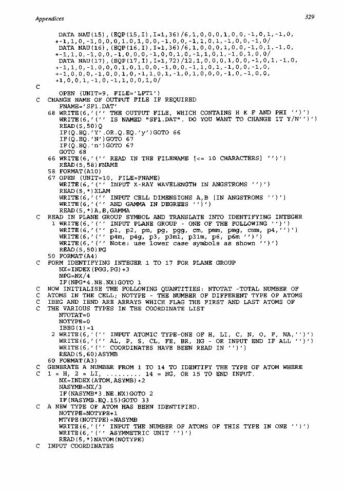
Appendices *29
DATA NAU(15), (EQP(15,I),1 = 1,36)/6,1,0,0,0,1,0,0,-1,0,1,-1,0,+-1,1,0,-1,0,0,0,1,0,1,0,0,-1,0,0,-1,1,0,1,-1,0,0,-1,0/DATA NAU(16),(EQP(16,I),1=1,36)/6,1,0,0,0,1,0,0,-1,0,1,-1,0,+-1,1,0,-1,0,0,-1,0,0,0,-1,0,0,1,0,-1,1,0,1,-1,0,1,0,0/DATA NAU(17),(EQP(17,I),1=1,72)/12,1,0,0,0,1,0,0,-1,0,1,-1,0,+-1,1,0,-1,0,0,0,1,0,1,0,0,-1,0,0,-1,1,0,1,-1,0,0,-1,0,+-1,0,0,0,-1,0,0,1,0,-1,1,0,1,-1,0,1,0,0,0,-1,0,-1,0,0,+1,0,0,1,-1,0,-1,1,0,0,1,0/
cOPEN (UNIT=9, FILE='LPT1')
C CHANGE NAME OF OUTPUT FILE IF REQUIREDFNAME='SF1.DAT'
68 WRITE(6,'(" THE OUTPUT FILE, WHICH CONTAINS H K F AND PHI '')')WRITE(6,/(// IS NAMED "SF1.DAT". DO YOU WANT TO CHANGE IT Y/N'')')READ(5,50)QIF(Q.EQ.'Y'.OR.Q.EQ.'y')GOTO 66IF(Q.EQ.'N')GOTO 67IF(Q.EQ.'n')GOTO 67GOTO 68
66 WRITE(6,'('' READ IN THE FILENAME [<= 10 CHARACTERS] '')')READ(5,58)FNAME
58 FORMAT(A10)67 OPEN (UNIT=10, FILE=FNAME)
WRITE(6,'('' INPUT X-RAY WAVELENGTH IN ANGSTROMS '')')READ(5,*)XLAMWRITE(6,' (" INPUT CELL DIMENSIONS A,B [IN ANGSTROMS '')')WRITE(6, ' (' ' AND GAMMA IN DEGREES ' ')')READ(5,*)A,B,GAMMA
C READ IN PLANE GROUP SYMBOL AND TRANSLATE INTO IDENTIFYING INTEGER1 WRITE(6,'(" INPUT PLANE GROUP - ONE OF THE FOLLOWING '')')VIRITE{6,' {' ' pi, p2, pm, pg, pgg, cm, pmm, pmg, cmm, p4,'')')WRITE(6,'(" p4m, p4g, p3, p3ml, p31m, p6, p6m '')')WRITE(6,'(// Note: use lower case symbols as shown '')')READ (5, 50) PG
50 FORMAT(A4)C FORM IDENTIFYING INTEGER 1 TO 17 FOR PLANE GROUP
NX=INDEX(PGG,PG)+3NPG=NX/4IF(NPG*4.NE.NX)GOTO 1
C NOW INITIALISE THE FOLLOWING QUANTITIES: NTOTAT -TOTAL NUMBER OFC ATOMS IN THE CELL; NOTYPE - THE NUMBER OF DIFFERENT TYPE OF ATOMSC IBEG AND IEND ARE ARRAYS WHICH FLAG THE FIRST AND LAST ATOMS OFC THE VARIOUS TYPES IN THE COORDINATE LIST
NTOTAT=0NOTYPE=0IBEG(1)=1
2 WRITE(6,'('' INPUT ATOMIC TYPE-ONE OF H, LI, C, N, O, F, NA,'')')WRITE(6,'(" AL, P, S, CL, FE, BR, HG - OR INPUT END IF ALL ")')WRITE(6, ' (' ' COORDINATES HAVE BEEN READ IN " ) ')READ(5,60)ASYMB
60 FORMAT(A3)C GENERATE A NUMBER FROM 1 TO 14 TO IDENTIFY THE TYPE OF ATOM WHEREC 1 = H, 2 = LI, 14 = HG, OR 15 TO END INPUT.
NX=INDEX (ATOM, ASYMB) +2NASYMB=NX/3IF(NASYMB*3.NE.NX)GOTO 2IF(NASYMB.EQ.15)GOTO 33
C A NEW TYPE OF ATOM HAS BEEN IDENTIFIED.NOTYPE=NOTYPE+1MTYPE(NOTYPE)=NASYMBWRITE(6,'(" INPUT THE NUMBER OF ATOMS OF THIS TYPE IN ONE '')')WRITE(6, ' ( " ASYMMETRIC UNIT ' ') ')READ(5,*)NATOM(NOTYPE)
C INPUT COORDINATES

330 Appendices
WRITE(6,' (' ' INPUT COORDINATES X, Y - ONE ATOM PER LINE '')')WRITE(6,'('' IF YOU ENTER A COORDINATE INCORRECTLY THERE ")')WRITE(6,'(" IS AN OPPORTUNITY LATER TO CORRECT IT '')')DO 5 I=1/NATOM(NOTYPE)READ(5,*)XX,YY
C GENERATE COORDINATES OF ALL SYMMETRY RELATED ATOMSDO 5 J=1,NAU(NPG)NTOTAT=NTOTAT+1X(NTOTAT)=EQP(NPG,6*J-5)*XX+EQP(NPG,6*J-4)*YY+EQP(NPG,6*J-3)Y(NTOTAT) =EQP(NPG, 6*J-2)*XX+EQP(NPG, 6*J-1) *YY+EQP(NPG, 6*J)
5 CONTINUEIEND(NOTYPE)=NTOTATIBEG(NOTYPE+1)=NTOTAT+1
C IF THIS ATOMIC TYPE IS AN ANOMALOUS SCATTERER THEN THE REAL ANDC IMAGINARY PARTS OF THE ANOMALOUS COMPONENT OF THE SCATTERINGC FACTOR MUST BE GIVEN
16 WRITE(6,'('' IS THIS TYPE AN ANOMALOUS SCATTERER? Y/N'')')READ(5,50)QIF(Q.EQ.'Y '.OR.Q.EQ.'y ')GOTO 6IF(Q.EQ.'N ')GOTO 2IF(Q.EQ.'n ')GOTO 2GOTO 16
6 WRITE(6,'(" INPUT REAL AND IMAGINARY PART OF A.S FACTOR'')')READ(5,*)FP(NOTYPE), FPP(NOTYPE)GOTO 2
C AT THIS STAGE ALL ATOMIC COORDINATES HAVE BEEN INPUTC IN CASE OF ERROR THEY MAY NOW BE DISPAYED WITH A POSSIBILITYC OF CHANGING ANY INCORRECT ONE
33 WRITE(6,'('' DO YOU WANT TO INSPECT THE COORDINATES? Y/N ")')READ(5/50)QIF(Q.EQ.'Y'.OR.Q.EQ.'y')GOTO 80IF(Q.EQ.'N')GOTO 3IF(Q.EQ.'n')GOTO 3GOTO 33
80 DO 90 1=1,NTOTAT,NAU(NPG)WRITE(6/200)X(I)#Y(I)
200 FORMAT(2F8.4)70 WRITE(6/'(" DO YOU WANT TO CHANGE THIS? Y/N'')')
READ(5,50)QIF(Q.EQ.'Y'.OR.Q.EQ.'y')GOTO 71IF(Q.EQ.'N')GOTO 90IF(Q.EQ.'n')GOTO 90GOTO 70
71 WRITE(6,'('' INPUT REPLACEMENT X,Y '')')READ (5 , * ) XX, YYDO 72 J=1,NAU(NPG)X(I+J-l)=EQP(NPG,6*J-5)*XX+EQP(NPG,6*J-4)*YY+EQP(NPG,6*J-3)
72 Y(I+J-1)=EQP(NPG,6*J-2)*XX+EQP(NPG,6*J-1)*YY+EQP(NPG,6*J)90 CONTINUE3 WRITE(6/'('
/ INPUT TEMPERATURE FACTOR. IF ONE IS NOT '')')WRITE(6,'('' REQUIRED THEN INPUT 0 '')')READ(5,*)BTEMP
C PROVIDE A TEST QUANTITY FOR THE PRESENCE OF ANOMALOUS SCATTERINGTESTAS=0DO 7 1=1,NOTYPE
7 TESTAS=TESTAS+FP(I)**2+FPP(I)**2C ALL INPUT IS NOW COMPLETE. NOW STRUCTURE FACTORS ARE CALCULATEDC TO THE LIMIT OF RESOLUTION GIVEN BY THE X-RAY WAVELENGTH.C NORMALLY A COMPLETE SEMICIRCLE OF STRUCTURE FACTORS WILL BEC CALCULATED ALTHOUGH THE ASYMMETRIC UNIT OF RECIPROCAL SPACEC MAY BE SMALLER THAN THIS. CALCULATIONS ARE FOR ALL INDEPENDENTC REFLECTIONS WITH k >= 0. IF ANOMALOUS SCATTERING IS PRESENT THENC THE COMPLETE CIRCLE IS CALCULATED. FIRST CALCULATE MAXIMUM INDICES.
HMAX=INT(2.0*A/XLAM)

Appendices 331
KMAX=INT(2.O*B/XLAM)C C01, CO2 AND CO3 ARE USED FOR CALCULATING SIN(THETA)/LAMBDA
COl=0.25/A/ACO2=0.25/B/BCO3=0.5/A/B*COS(GAMMA*0.0174533)
C SLIM IS THE LIMITING VALUE OF (SIN(THETA)/LAMBDA)**2 AND NOREFC RECORDS THE TOTAL NUMBER OF REFLECTIONS.
SLIM=1/XLAM/XLAMNOREF=0DO 10 H=-HMAX,HMAXDO 10 K=0,KMAXIF(K.EQ.0.AND.H.LT.0)GOTO 10
C NOW CALCULATE (SIN(THETA)/LAMBDA)**2 AND CHECK THAT < SLIMSL2=CO1*H*H+CO2*K*K-CO3*H*KIF(SL2.GT.SLIM)GOTO 10SL=SQRT(SL2)
C NOW THE STRUCTURE FACTOR IS CALCULATED. IF THERE IS ANOMALOUSC SCATTERING THEN BOTH F(h k 1) AND F(-h -k -1) ARE CALCULATED.
SUMA=0SUMB=0SMAASP=0SMAASM=0SMBASP=0SMBASM=0DO 15 I=1,NOTYPE
C CALL SUBROUTINE TO DERIVE SCATTERING FACTOR [SCF] FOR ATOMC OF TYPE I FOR SIN(THETA)/LAMBDA = SL
CALL SCAT(MTYPE(I)fSLfSCF)PSUMA=0PSUMB=0
C CALCULATE CONTRIBUTIONS TO REAL AND IMAGINARY PARTS OF THEC STRUCTURE FACTOR OF ATOMS OF TYPE I
DO 26 J=IBEG(I),IEND(I)Z=6.2 831853*(H*X(J)+K*Y(J))PSUMA=PSUMA+COS(Z)
26 PSUMB=PSUMB+SIN(Z)SUMA=SUMA+SCF*PSUMASUMB=SUMB+SCF*PSUMB
C TEST FOR PRESENCE OF ANOMALOUS SCATTERINGIF(TESTAS.LT.1.0E-12)GOTO 15
C TEST FOR ATOM TYPE I AS ANOMALOUS SCATTERERIF(FP(I)**2+FPP(I)**2.LT.1.0E-12)GOTO 15SMAASP=SMAASP+PSUMA*FP(I)-PSUMB*FPP(I)SMAASM=SMAASM+PSUMA*FP(I)+PSUMB*FPP(I)SMBASP=SMBASP+PSUMB*FP(I)+PSUMA*FPP(I)SMBASM=SMBASM-PSUMB*FP(I)+PSUMA*FPP(I)
15 CONTINUENOREF=NOREF+1HT(NOREF)=HKT(NOREF)=KBTFAC=1.0IF(BTEMP.GT.1.0E-12)BTFAC=EXP(-BTEMP*SL2)F(NOREF)=SQRT((SUMA+SMAASP)**2 +(SUMB+SMBASP)**2)*BTFACPHI(NOREF)=ATAN2(SUMB+SMBASP,SUMA+SMAASP)*57.2958IF(F(NOREF).LT.1.0E-4)PHI(NOREF)=0IF(TESTAS.LT.1.0E-12)GOTO 10NOREF=NOREF+1HT(NOREF)=-HKT(NOREF)=-KF(NOREF)=SQRT((SUMA+SMAASM)**2 +(-SUMB+SMBASM)**2)*BTFACPHI(NOREF)=ATAN2(-SUMB+SMBASM,SUMA+SMAASM)*57.2958IF(F(NOREF).LT.1.OE-4)PHI(NOREF)=0
10 CONTINUEWRITE(10,*)NOREF,(HT(I),KT(I),F(I),PHI(I),1=1,NOREF)

332 Appendices
WRITE(9,700)700 FORMAT(3(24H h k F PHI ))
WRITE(9,100)(HT(I),KT(I),F(I),PHI(I),I=1,NOREF)100 FORMAT(3(16,14,F8.2,F6.0))
STOPEND
SUBROUTINE SCAT(I,SL,SCF)C THERE NOW FOLLOW THE SCATTERING FACTORS FROM INTERNATIONAL TABLESC FOR ATOMS H, LI, C, N, O, NA, AL, P, S, CL, FE, BR AND HG ATC INTERVALS OF 0.1 FOR SIN(THETA)/LAMBDA. PARABOLIC INTERPOLATION ISC USED TO OBTAIN THE SCATTERING FACTOR FOR SIN(THETA)/LAMBDA = SL.
DIMENSION SF(14,0:10)DATA (SF(1,I),1=0,10)/I.000,0.811,0.481,0.251,0.130,0.071,+0.040,0.024,0.015,0.010,0.007/DATA (SF(2,I),1=0,10)/3.000,2.215,1.741,1.521,1.269,1.032,+0.823,0.650,0.513,0.404,0.320/DATA (SF(3,I),1=0,10)/6.000,5.126,3.581,2.502,1.950,1.685,+1.53 6,1.42 6,1.322,1.218,1.114/DATA (SF(4,I),1=0,10)/7.000,6.203,4.600,3.241,2.397,1.944,+1.698,1.550,1.444,1.350,1.263/DATA (SF(5,I),1=0,10)/8.000,7.250,5.634,4.094,3.010,2.338,+1.944,1.714,1.566,1.462,1.374/DATA (SF(6,I),1=0,10)/9.000,8.293,6.691,5.044,3.760,2.878,+2.312,1.958,1.735,1.587,1.481/DATA (SF(7,I),1=0,10)/ll.00,9.76,8.34,6.89,5.47,4.29,3.40,+2.76,2.31,2.00,1.78/DATA (SF(8,I),1=0,10)/13.00,11.23,9.16,7.88,6.72,5.69,4.71,+3.88,3.21,2.71,2.32/DATA (SF(9,I),1=0,10)/l5.00,13.17,10.34,8.59,7.54,6.67,5.83,+5.02,4.28,3.64,3.11/DATA (SF(10,I),1=0,10)/l6.00,14.33,11.21,8.99,7.83,7.05,6.31,+5.56,4.82,4.15,3.56/DATA (SF(11,I),1=0,10)/l7.00,15.33,12.00,9.44,8.07,7.29,6.64,+5.96,5.27,4.60,4.00/DATA (SF(12,I),1=0,10)/26.00,23.68,20.09,16.77,13.84,11.47,+9.71,8.47,7.60,6.99,6.51/DATA (SF(13,I),1=0,10)/35.00,32.43,27.70,23.82,20.84,18.27,+15.91,13.78,11.93,10.41,9.19/DATA (SF(14,I),1=0,10)/80.00,75.48,67.14,59.31,52.65,47.04,+42.31,38.22,34.64,31.43,28.59/J=INT(SL/0.1)IF(J.EQ.IO)J=9IF(J.EQ.O)J=lA=(SF(I,J+1)+SF(I,J-l)-2*SF(I,J))/0.02B=(SF(I,J+l)-SF(I,J-l))/0.2SCF=A*(SL-0.1*J)**2+B*(SL-0.1*J)+SF(I,J)RETURNEND
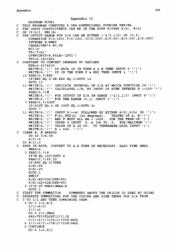
Appendices 333
Appendix IIPROGRAM FOUR1
C THIS PROGRAM COMPUTES A ONE-DIMENSIONAL FOURIER SERIES.C THE INPUT COEFFICIENTS CAN BE IN THE FORM EITHER A(h), B(h)C OR |F(h)|, PHI(h).C THE OUTPUT RANGE FOR X/A CAN BE EITHER (-1/2,1/2) OR (0,1).
DIMENSION X(0:100) ,Y(0:100) ,IC(0:200) ,A(0:50) ,B(0:50) ,Z (0:200)INTEGER H,HMAXCHARACTER*4 NC,FXNC='n'FX='f(x)'OPEN(UNIT=9,FILE='LPT1' )TPI=6.2831853
C CONSTANT TO CONVERT DEGREES TO RADIANSDTR=0.0174533WRITE(6,'(" IF DATA IS IN FORM A & B THEN INPUT 0 '')')WRITE(6,'('' IF IN THE FORM F & PHI THEN INPUT 1 '')')
13 READ (5,*) KEYIF(KEY.EQ.0.OR.KEY.EQ.l)GOTO 12GOTO 13
12 WRITE(6,'(" INDICATE INTERVAL OF X/A AT WHICH FUNCTION IS'7)7)WRITE(6,'('' CALCULATED,1/N, BY INPUT OF EVEN INTEGER N <=200//)/)READ(5,*)NWRITE(6, ' (" FOR OUTPUT OF X/A IN RANGE (-1/2,1/2) INPUT 0'')')WRITE(6, ' (' ' FOR THE RANGE (0,1) INPUT 1'')')
7 READ (5, *) IOUTIF(IOUT.EQ.0.OR.IOUT.EQ.1)GOTO 11GOTO 7
11 WRITE(6,/('/ INPUT h(+ve) FOLLOWED BY EITHER A(h),B(h) OR '')')WRITE(6,'(" F(h),PHI(h) [in degrees]. VALUES OF A, B'')')WRITE(6,/(// AND F MUST ALL BE < 1000. FOR THE TERM OF'')')WRITE(6,'(" INDEX 0 INPUT 0, A [OR F] , 0. THE MAXIMUM'')')WRITE(6, ' (' ' VALUE OF h IS 50. TO TERMINATE DATA INPUT' ') ')WRITE (6, ' (' ' H = 100. ")')
C CLEAR A, B ARRAYSDO 50 1=0,50A(I)=0
50 B(I)=0C READ IN DATA. CONVERT TO A,B FORM IF NECESSARY. ALSO FIND HMAX.
HMAX=03 READ(5,*)HIF(H.EQ.100)GOTO 4READ(5,*)XX,YYIF(KEY.EQ.0)THENA(H)=XXB(H)=YYGOTO 2ENDIFA(H)=XX*COS(DTR*YY)B(H)=XX*SIN(DTR*YY)
2 IF(H.GT.HMAX)HMAX=HGOTO 3
C START THE SUMMATION. SYMMETRY ABOUT THE ORIGIN IS USED BY DOINGC SEPARATE SUMMATIONS FOR THE COSINE AND SINE TERMS FOR X/A FROMC 0 TO 1/2 AND THEN COMBINING THEM.
4 DO 5 1=0,N/2X(I)=A(0)Y(I)=0DO 6 J=1,HMAXARG=TPI*FLOAT(J*I)/NX(I)=X(I)+2*A(J)*COS(ARG)
6 Y(I)=Y(I)+2*B(J)*SIN(ARG)5 CONTINUEDO 8 1=0,N/2

334 Appendices
IF(IOUT.EQ.0)THENIC(I)=I-N/2Z(I)=X(N/2-I)-
Z(N-l)=X(N/2-I)+Y(N/2-I)GOTO 8ENDIF
IC(N-I)=N-IZ(N-I)=X(I)-
8 CONTINUECALCULATION COMPLETE. OUTPUT STAGE BEGINS.
WRITE(9,100)N100 F0RMAT(41H THE COORDINATES ARE X/A = n/N WHERE N = ,13)
WRITE(9,' (' ' '')')WRITE(9,150)NC,FX,NC,FX,NC,FX,NC,FX
150 FORMAT(4(6X,A4,IX,A4))WRITE(9,2 00)(IC(I),Z(I),1=0,N)
200 FORMAT(4(18,F7.2))STOPEND
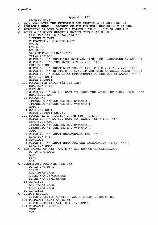
Appendices 335
Appendix IIIPROGRAM SIMP1
C THIS EVALUATES THE INTEGRALS FOR FINDING A(h) AND B(h) BYC SIMPSON'S RULE. BECAUSE OF THE PERIODIC NATURE OF f(x) THEC SUMMATION IS DONE OVER THE POINTS 0 TO N-l (NOT N) AND THEC POINT 0 IS GIVEN WEIGHT 2 RATHER THAN 1 AS USUAL.
REAL F(0:199)fA(0:50)fB(0:50)INTEGER H,HMAXCHARACTER*4 HC,AC,BC#ANS*1HC='h'AC='A(h)'BC='B(h)'OPEN(UNIT=9,FILE='LPT1')TPI=6.2831853WRITE(6,' (' ' INPUT THE INTERVAL, l/N, FOR QUADRATURE AS AN'')')WRITE(6,'('' EVEN INTEGER N <= 200 '')')READ(5,*)NNWRITE(6,'('' INPUT N VALUES OF f(x) FOR x = 0 TO 1-l/N '')')WRITE(6,'('' IN STEPS OF l/N. IF YOU MAKE AN ERROR THERE '')')WRITE(6,'(" WILL BE AN OPPORTUNITY TO CORRECT IT LATER. '')')DO 1 I=0/NN-lWRITE(6,100)I
100 FORMAT(11H INPUT f{X[,I3,lH])READ(5,*)F (I)
1 CONTINUE3 WRITE(6,'('' DO YOU WANT TO CHECK THE VALUES OF f(x)? Y/N ")')READ(5,25)ANS
25 FORMAT(Al)IF(ANS.EQ.'N'.OR.ANS.EQ.'n')GOTO 2IF(ANS.EQ.'Y'.OR.ANS.EQ.'y')GOTO 4GOTO 3
4 DO 5 I=0,NN-lWRITE(6,200)I,NN,F(I)
200 FORMAT(4H X =,14,1H/,13,7H f(x) =,F6.2)7 WRITE(6, ' (' ' DO YOU WANT TO CHANGE THIS? Y/N " ) ')READ(5,25)ANSIF(ANS.EQ.'N'.OR.ANS.EQ.'n')GOTO 5IF(ANS.EQ.'Y'.OR.ANS.EQ.'y')GOTO 6GOTO 7
6 WRITE(6,' ('' INPUT REPLACEMENT f(x) '')')READ(5f*)F(I)
5 CONTINUE2 WRITE(6,'('' INPUT HMAX FOR THE CALCULATION [<=50] '')')READ(5,*)HMAX
C THE VALUES OF A(h) AND B(h) ARE NOW TO BE CALCULATEDDO 10 H=0,HMAXAA=0BB=0W=4
C SUMMATIONS FOR A(h) AND B(h)DO 12 J=07NN-lW=6-WARG=TPI*H*J/NNAA=AA+W*F(J)*COS(ARG)BB=BB+W*F(J)*SIN(ARG)
12 CONTINUEA(H)=AA/3.0/NNB(H)=BB/3.0/NN
10 CONTINUEC OUTPUT RESULTS
150 F0RMAT(4 (4X^4^4, 3X,A4) )WRITE(9,250)(I#A(I),B(I),1=0,HMAX)
250 FORMAT(4(15,2F7.2))STOP

336 Appendices
Appendix IVPROGRAM FOUR2
C FOUR2 CALCULATES A TWO-DIMENSIONAL PROJECTED ELECTRON DENSITY MAPC FROM STRUCTURE FACTORS INPUT FROM THE OUTPUT FILE OF STRUCFAC.C THE DENSITY IS SCALED TO A MAXIMUM VALUE OF 100 AND THE SCALINGC FACTOR TO CONVERT TO ELECTRONS/ANGSTROM**2 IS GIVEN. TO TAKEC ACCOUNT OF THE LIMITED WIDTH OF PRINTER PAPER THE OUTPUT IS INC SECTIONS WHICH HAVE TO BE JOINED SIDEWAYS. FOR ECONOMY THEC OUTPUT IS ON AN ORTHOGONAL GRID AND THE SCALING WILL NOT BEC ACCURATE ALONG THE AXES. THE VALUES OF HMAX AND HMIN MUST BEC <= 15 AND THE MINIMUM GRID SPACING IS 1/60.C THERE IS A PATTERSON FUNCTION OPTION IN WHICH CASE THE SCALINGC FACTOR IS ELECTRONS**2/ANGSTROM**2.
DIMENSION A(-15:15,0:15), B(-15115,0:15),AC(0:15,0:30),+AS(0:15,0:30),BC(0:15,0:30),BS(0:15,0:30),CSX(0:60),+CSY(0:60),RO(0:60,0:60),LIST(0:60),HH(500),KK(500),+F(500),PHI(500)INTEGER H,HHCHARACTER ANS*1,FNAME*10,DIR*1,BT*6DATA NPAGE/15/OPEN(UNIT=9,FILE='LPT1')TPI=6.2831853
C CONSTANT FOR CONVERTING DEGREES TO RADIANSDTR=0.0174533
C CLEAR A AND B ARRAYSDO 1 H=-15,15DO 1 K=0,15A(H,K)=0B(H,K)=0
1 CONTINUEFNAME=/SF1.DAT/
4 WRITE(6,' (' ' IT IS ASSUMED THAT THE INPUT DATA FILE IS NAMED'')')WRITE(6,' (' ' SF1.DAT. DO YOU WISH TO CHANGE THE NAME? Y/N'')')READ(5,50)ANS
50 FORMAT(Al)IF(ANS.EQ.'N'.OR.ANS.EQ.'n')GOTO 2IF(ANS.EQ.'Y'.OR.ANS.EQ.'y')GOTO 3GOTO 4
3 WRITE(6,'(" READ IN FILENAME [<= 10 CHARACTERS] '')')READ(5,55)FNAME
55 FORMAT(A10)2 OPEN(UNIT=10,FILE=FNAME)HMAX=0KMAX=0
C INPUT THE CELL DIMENSIONS A & B AND THE CELL ANGLE GAMMA.WRITE(6,'('' INPUT CELL DIMENSIONS A,B AND GAMMA (degrees)'')')WRITE(6,' (' ' MAKE SURE THAT THEY ARE CONSISTENT WITH THE '')')WRITE(6,'('' X,Y COORDINATES USED IN PROGRAM STRUCFAC. '')')READ(5,*)AA,BB,GAMMAAREA=AA*BB*SIN(DTR*GAMMA)READ(10,*)NOREF,(HH(I),KK(I),F(I),PHI(I),I=1,NOREF)
95 WRITE(6,'('' DO YOU WANT THE PATTERSON OPTION? Y/N '')')WRITE(6,'('' REMEMBER - IF THE INPUT TAPE IS FROM PROGRAM'')')WRITE(6,'('' ISOFILE THEN YOU SHOULD INPUT N '')')READ(5,50)ANSIF(ANS.EQ.'Y'.OR.ANS.EQ.'y')GOTO 93IF(ANS.EQ.'N'.OR.ANS.EQ.'n')GOTO 94GOTO 95
93 DO 96 I=1,NOREFF(I)=F(I)*F(I)PHI(I)=0
96 CONTINUE94 DO 77 I=1,NOREF
IF(ABS(HH(I)).GT.HMAX)HMAX=ABS(HH(I))
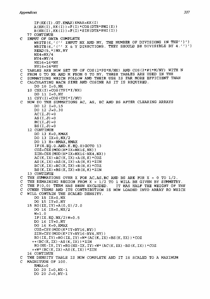
Appendices 337
IF(KK(I).GT.KMAX)KMAX=KK(I)A(HH(I),KK(I))=F(I)*COS(DTR*PHI(I))B(HH(I),KK(I))=F(I)*SIN(DTR*PHI(I))
77 CONTINUEC INPUT OF DATA COMPLETE
WRITE(6,' (" INPUT NX AND NY, THE NUMBER OF DIVISIONS IN THE'')')WRITE(6,'('' X Sc Y DIRECTIONS. THEY SHOULD BE DIVISIBLE BY 4.'')')READ (5,*) NX, NYNX4=NX/4NY4=NY/4NX16=16*NXNY16=16*NY
C TABLES ARE NOW SET UP OF COS(2*PI*N/NX) AND COS(2*PI*M/NY) WITH NC FROM 0 TO NX AND M FROM 0 TO NY. THESE TABLES ARE USED IN THEC SUMMATIONS WHICH FOLLOW AND THEIR USE IS FAR MORE EFFICIENT THANC CALCULATING EACH SINE AND COSINE AS IT IS REQUIRED.
DO 10 1=0,NX10 CSX(I)=COS(TPI*l/NX)
DO 11 1=0,NY11 CSY(I)=COS(TPI*I/NY)
C NOW DO THE SUMMATIONS AC, AS, BC AND BS AFTER CLEARING ARRAYSDO 12 1=0,15DO 12 J=0,30AC(I,J)=0AS(I,J)=0BC(I, J)=0BS(I, J)=0
12 CONTINUEDO 13 K=0,KMAXDO 13 IX=0,NX/2DO 13 H=-HMAX,HMAXIF(H.EQ.0.AND.K.EQ.0)GOTO 13COZ=CSX(MOD(H*IX+NX16,NX))ZIN=CSX(MOD(H*IX+NX16-NX4,NX))AC (K, IX) =AC (K, IX) +A (H, K) *COZAS (K, IX) =AS (K, IX) +A(H,K) *ZINBC (K, IX) =BC (K, IX) +B (H, K) *COZBS (K, IX) =BS (K, IX) +B(H,K) *ZIN
13 CONTINUEC THE SUMMATIONS OVER X FOR AC,AS,BC AND BS ARE FOR X = 0 TO 1/2.C THE REMAINING REGION FROM X = 1/2 TO 1 WILL BE GIVEN BY SYMMETRY.C THE F(0,0) TERM HAS BEEN EXCLUDED. IT HAS HALF THE WEIGHT OF THEC OTHER TERMS AND ITS CONTRIBUTION IS NOW LOADED INTO ARRAY RO WHICHC WILL CONTAIN THE SCALED DENSITY.
DO 15 IX=0,NXDO 15 IY=0,NY
15 RO(IX,IY)=A(0,0)/2.0DO 16 IX=0,NX/2W=1.0IF(IX.EQ.NX/2)W=0.5DO 16 IY=0,NYDO 16 K=0,KMAXCOZ=CSY(MOD(K*IY+NY16,NY))ZIN=CSY(MOD(K*IY+NY16-NY4,NY))RO(IX,IY)=RO(IX,IY)+W*(AC(K,IX)+BS(K,IX))*COZ+ +(BC(K,IX)-AS(K,IX))*ZINRO(NX-IX,IY)=RO(NX-IX,IY)+W*(AC(K,IX)-BS(K,IX)) *COZ++W*(BC(K,IX)+AS(K,IX))*ZIN
16 CONTINUEC THE DENSITY TABLE IS NOW COMPLETE AND IT IS SCALED TO A MAXIMUMC MAGNITUDE OF 100.
RMAX=0DO 20 I=0,NX-lDO 20 J=0,NY-l

Appendices
IF(ABS(RO(I, J) ) .GT.RMAX)RMAX=ABS(RO(I, J) )2 0 CONTINUE
FAC=100/RMAXDO 21 1=0,NXDO 21 J=0,NYRO(I,J)=FAC*RO(I,J)
21 CONTINUEC CALCULATE FACTOR WHICH GIVES PROJECTED DENSITY FROM PRINTED VALUES
CAF=1/FAC/AREAC OUTPUT THE FACTOR
WRITE(9,700)CAF700 FORMAT(42H FACTOR CONVERTING TO DENSITY/UNIT AREA IS,F8.4)
DO 66 1=0,60LIST(I)=I
66 CONTINUEC FIND A CONVENIENT ORIENTATION FOR THE OUTPUT WHICH IS THAT WITHC THE LEAST NUMBER OF DIVISIONS ACROSS THE PAGE.
DIR='X'BT='BOTTOM'M=NX/NPAGE+1L=0IF(NY.LT.NX)THENDIR='Y'BT=' TOP'M=NY/NPAGE+1L=lENDIFWRITE(9,100)DIR,BT
100 FORMAT(13H OUTPUT WITH ,A1,23H HORIZONTAL AND ORIGIN ,A6,5H LEFT)IF(L.EQ.1)GOTO 30
C THE MAP IS PRINTED IN SECTIONS WHICH MUST BE JOINED AT SIDE EDGES.C THE NUMBER OF GRIDPOINTS ACROSS THE PAGE IS NPAGE WHICH IS SET ATC 15. FOR OTHER AVAILABLE PAGE WIDTHS THIS CAN BE ALTERED BY THEC DATA STATEMENT NEAR THE BEGINNING OF THE PROGRAM.
DO 25 N0=l,MWRITE(9,'('' '')')WRITE(9,'('' '')')Nl=(N0-l)*NPAGEN2=NPAGE*N0IF(N0.EQ.M)N2=NXWRITE(9,150)(LIST(I),I=N1,N2)
150 FORMAT(5X,2114)WRITE(9, ' (' ' " ) ')DO 25 IY=NY,0,-1WRITE(9,200)IY,(RO(IX,IY),IX=N1,N2)
200 FORMAT(I4,2X,21F4.0)WRITE(9,'('' '')')
25 CONTINUEGOTO 45
30 DO 26 N0=l,MWRITE(9,'('' '')')WRITE(9,'('' '')')Nl=(N0-l)*NPAGEN2=NPAGE*N0IF(N0.EQ.M)N2=NYWRITE(9,150)(LIST(I),I=N1,N2)WRITE(9,'('' '')')DO 2 6 IX=0,NXWRITE(9,200)IX,(RO(IX,IY),IY=N1,N2)WRITE(9,'('' '')')
2 6 CONTINUE45 STOP
END

Appendices 339
Appendix VPROGRAM FTOUE
C THIS PROGRAM ACCEPTS THE OUTPUT FROM STRUCFAC AND CONVERTS THEC F's INTO EITHER U'S OR E'S. THE F'S ARE FIRST SORTED INTO GROUPSC OF ROUGHLY 40 IN ORDER OF INCREASING VALUE OF SIN(THETA). FORC EACH GROUP A CONVERSION FACTOR IS FOUND WHICH WILL, FOR U'S, MAKEC <|U**2|>= SIGMA(f**2)/(SIGMA(f))**2 OR, FOR E'S MAKE <|E**2|> = 1.C THESE FACTORS ARE THEORETICALLY WHAT IS REQUIRED TO CONVERT F**2 TOC U**2 OR E**2 AT <SIN(THETA)> FOR EACH GROUP. A BEST FIT OF THEC KIND " FACTOR = C(1)+C(2)*S+C(3)*S**2 " [s = SIN(THETA)] IS FOUNDC TO FIT THE CONVERSION FACTORS AND <SIN(THETA)> FOR EACH GROUP.C THE QUADRATIC FORMULA IS THEN USED WITH THE S FOR EACH REFLECTIONC TO CONVERT THE VALUE OF F TO U OR E. THESE ARE THEN PLACED IN AC FILE UE.DAT FOR SUBSEQUENT USE.
REAL F(1000),THETLIST(100),F2LIST(100),AVSUMF2(30),AVTHET(30),+EPS(30),C(3),UE(1000)INTEGER ISYMB(13),NATOM(13),HT(1000),KT(1000),NUMLIST(100),
+IEND(0:30)CHARACTER Q*4,FNAME*10,ASYMB*3,CU*1,ATOM*(*)PARAMETER (ATOM='H LI C N 0 NA AL P S CL FE BR HG END')OPEN(UNIT=9,FILE='LPT1')FNAME='UE.DAT'WRITE(6,'('' THE OUTPUT FILE WHICH CONTAINS H,K,U (or E) IS'')')WRITE(6,'('' NAMED UE.DAT. DO YOU WANT TO CHANGE IT? (Y/N)'')')
3 READ(5,50)QIF(Q.EQ.'Y'.OR.Q.EQ.'y')GOTO 1IF(Q.EQ.'N'.OR.Q.EQ.'n')GOTO 2GOTO 3
1 WRITE(6,'('' READ IN THE FILENAME [<= 10 CHARACTERS] '')')READ(5,75)FNAME
50 FORMAT(A4)75 FORMAT(A10)2 OPEN(UNIT=10,FILE=FNAME)
C INPUT THE UNIT CELL DATAWRITE(6,'('' INPUT CELL DIMENSIONS A, B [IN ANGSTROMS] AND'')')WRITE(6, ' (' ' GAMMA IN DEGREES. " ) ')READ(5,*)A,B,GAMMA
C NOW CALCULATE FACTORS WHICH WILL BE USED LATER TO FIND VALUESC OF SIN[THETA]/LAMDA
COl=0.25/A/ACO2=0.25/B/BCO3=0.5/A/B*COS(GAMMA*0.0174533)WRITE(6,'('' INPUT THE RADIATION WAVELENGTH IN ANGSTROMS'')')READ(5,*)XLAM
C DECIDE WHETHER TO OUTPUT U'S OR E'S.WRITE(6,'('' DO YOU WANT U OR E? (U/E) '')')READ(5,50)QIF(Q.EQ.'U'.OR.Q.EQ.'u')THENIUE = 1GOTO 4ENDIFIF(Q.EQ.'E'.OR.Q.EQ.'e')THENIUE=2GOTO 4ENDIF
C INPUT THE ATOMIC CONTENTS OF THE WHOLE UNIT CELL4 WRITE(6,'('' THE CONTENTS OF THE WHOLE UNIT CELL [NOT JUST'')')
WRITE(6,'('' ONE ASYMMETRIC UNIT] IS INPUT IN THE FORM X1,N1")')WRITE(6,'('' X2,N2,ETC WHERE XI IS THE TYPE OF ATOM, WHICH '')')WRITE(6, ' (' ' MUST BE ONE OF H,LI,C,N,O,NA,AL,P,S,CL,FE,BR,HG, " ) ')WRITE(6,'('' AND Nl IS THE TOTAL NUMBER OF THAT TYPE. '')')WRITE(6,'('' '')')ITOT=0
6 WRITE(6,'('' INPUT ATOMIC TYPE'')')

340 Appendices
WRITE(6,'('' IF ALL ATOMS HAVE BEEN INPUT THEN INPUT END'')')READ(5,100)ASYMB
100 FORMAT(A3)NX=INDEX(ATOM,ASYMB)+2NASYMB=NX/3IF(NASYMB*3.NE.NX)GOTO 6IF(NASYMB.EQ.14)GOTO 7ITOT=ITOT+1ISYMB(ITOT)=NASYMBWRITE(6,'('' INPUT NUMBER OF ATOMS OF THIS TYPE IN WHOLE CELL'')')READ(5,*)NATOM(ITOT)GOTO 6
C THE DATA FROM STRUCFAC CAN NOW BE READ IN7 FNAME='SF1.DAT'
10 WRITE(6,'('' THE OUTPUT FILE FROM STRUCFAC IS ASSUMED TO BE'')')WRITE(6/
/(// NAMED SF1.DAT. DO YOU WANT TO CHANGE THIS? (Y/N)'')')READ(5,50)QIF(Q.EQ.'Y' .OR.Q.EQ.'y')GOTO 8IF(Q.EQ.'N'.OR.Q.EQ.'n')GOTO 9GOTO 10
8 WRITE(6, ' (" INPUT THE FILE NAME YOU WANT [<= 10 CHARACTERS] " ) ')READ (5, 75) FNAME
9 OPEN(UNIT=11/FILE=FNAME)READ(11,*)NOREF,(HT(I),KT(I),F(I),DUMMY,1=1,NOREF)
C EACH REFLECTION IS READ IN AND VALUES OF NUMBER OF REFLECTIONSC SIGMA(F**2) AND SIGMA(SIN[THETA]) ARE FOUND FOR SIN[THETA] RANGESC OF 0.01. REFLECTIONS WITH SIN[THETA] LESS THAN O.O5 ARE EXCLUDEDC SINCE THEY DISTURB THE STATISTICS. FIRST ALL ARRAYS ARE CLEARED
DO 66 1=1,100THETLIST(I)=0F2LIST(I)=0NUMLIST(I)=0
66 CONTINUEDO 20 1=1,NOREFSTHET=XLAM*SQRT(CO1*HT(I)**2+CO2*KT(I)**2-CO3*HT(I)*KT(I))IF(STHET.LT.0.05)GOTO 20ITG=INT(100*STHET)+lIF(ITG.GT.IOO)ITG=100THETLIST(ITG)=THETLIST(ITG)+STHETF2LIST(ITG)=F2LIST(ITG)+F(I) **2NUMLIST(ITG)=NUMLIST(ITG)+ 1
2 0 CONTINUEC NOW FIND GROUPS OF 40 OR SO FOR FINDING AVERAGESC THESE GROUPS WILL SLIGHTLY OVERLAP
DO 21 1=1,30IEND(I)=0
21 CONTINUEIEND(0)=lIX = 1IN=1
31 SUM=0DO 30 I=IN,100SUM=SUM+NUMLIST(I)IF(SUM.GE.40)THENIEND(IX)=IIX=IX+1IN=IIF(IN.EQ.100)GOTO 30GOTO 31ENDIF
3 0 CONTINUEC IF THE FINAL GROUP HAS MORE THAN 2 0 MEMBERS THEN IT IS ACCEPTEDC OTHERWISE IT IS ADDED TO THE PREVIOUS GROUP
IF(SUM.LT.20)IX=IX-1

Appendices 341
IEND(IX)=100C THE TOTAL NUMBER OF GROUPS IS IX. THE BEGINNINGS AND ENDS OF THEC GROUPS ARE IEND(O) TO IEND(l), IEND(l) TO IEND(2)C ...., IEND(IX-l) TO IEND(IX). NOW THERE ARE CALCULATED THE AVERAGEC F**2 IN EACH GROUP AND <SIN[THETA]>.
DO 40 1=1,IXSUMF2=0SUMTHET=0NSUM=0DO 41 J=IEND(I-1),IEND(I)SUMF2=SUMF2+F2LIST(J)SUMTHET=SUMTHET+THETLIST(J)NSUM=NSUM+NUMLIST(J)
41 CONTINUEAVSUMF2(I)=SUMF2/NSUMAVTHET(I)=SUMTHET/NSUM
40 CONTINUEC NOW CALCULATE CONVERSION FACTORS FOR CALCULATION OF U OR E
DO 60 1=1,IXSTLAM=AVTHET(I)/XLAMIF(IUE.EQ.2)THENFACTOR=SQRT(1.0/AVSUMF2(I))GOTO 62ENDIFSUM1=OSUM2=0DO 61 J=l,ITOTIA=ISYMB(ITOT)CALL SCAT(IA,STLAM,SCF)SUMl=SUMl+NATOM(J)*SCFSUM2=SUM2+NATOM(J)*SCF*SCF
61 CONTINUEFACTOR=SQRT(SUM2/AVSUMF2(I))/SUMl
62 EPS(I)=FACTOR60 CONTINUE
C A BEST PARABOLIC FIT IS NOW TO BE FOUND TO GIVE EPS AS A FUNCTIONC OF SIN[THETA]/LAMDA [=s].
CALL PARAFIT(AVTHET,EPS,IX,C)C C(l)+C(2)*s+C(3)*s*S GIVES THE CONVERSION FACTOR FROM F TO U OR EC THE PROPER VALUE OF E(0,0) OR U(0,0) IS KNOWN AND IS NOW CALCULATED
94 WRITE(6,'('' DO YOU WANT TO OUTPUT THE VALUES OF a, b AND c '')')WRITE(6,'('' GIVEN IN EQUATION 2.48? Y/N '')')READ(5,50)QIF(Q.EQ.'Y'.OR.Q.EQ.'y')THENIABC=1GOTO 93ENDIFIF(Q.EQ.'N'.OR.Q.EQ.'n')THENIABC=0GOTO 93ENDIFGOTO 94
93 IF(IUE.EQ.1)THENZ = 1.0GOTO 89ENDIFSUM1=OSUM2=0DO 87 1=1,ITOTNN=ISYMB(I)CALL SCATFAC(NN,0.0,SCF)SUM1=SUM1+NATOM(I)*SCFSUM2=SUM2+NATOM(I)*SCF**2
87 CONTINUE
542 Appendices
Z=SUM1/SQRT(SUM2)C FIND E(0)
89 DO 90 I=1,NOREFIF(HT(I).EQ.O.AND.KT(I).EQ.0)THENUE(I)=ZGOTO 90ENDIF
90 CONTINUEDO 91 I=1,NOREFIF(HT(I).EQ.O.AND.KT(I).EQ.0)GOTO 91STHET=XLAM*SQRT(CO1*HT(I)**2+CO2*KT(I)**2-CO3*HT(I)*KT(I))CONV=C(1)+C(2)*STHET+C(3)*STHET**2UE(I)=CONV*F(I)
C CHECK THAT THE CALCULATED E IS NOT BIGGER THAN E(0) WHICH CANC HAPPEN FOR A LARGE STRUCTURE FACTOR TAKING INTO ACCOUNT THEC INACCURACIES IN SCALING.
IF(UE(I).GT.0.95*Z)UE(I)=0.95*Z91 CONTINUE
C ALL F's HAVE NOW BEEN CONVERTED TO U OR E. THEY ARE NOW WRITTEN ONC A FILE FOR FUTURE USE.
WRITE(10,*)IUE,NOREF,(HT(I),KT(I),UE(I),I=1/NOREF)C THE VALUES OF a, b AND c ARE WRITTEN IF REQUESTED
IF(IABC.EQ.0)GOTO 95WRITE(9,500)C
500 FORMAT(5H a = ,E9.3,5H b = ,E9.3,5H c = ,E9.3)95 CU='U'
IF(IUE.EQ.2)CU='E'WRITE(9,200)CU
200 FORMAT(11H VALUES OF ,A1)WRITE(9,300)CU,CU,CU
300 FORMAT(3(16H H K ,A1,3X))WRITE(9,400)(HT(I),KT(I),UE(I),I=1,NOREF)
400 FORMAT(3(5X,I3,I5,F7.3))STOPEND
SUBROUTINE SCATFAC(I,SL,SCF)C THERE NOW FOLLOW THE SCATTERING FACTORS FROM INTERNATIONAL TABLESC FOR ATOMS H, LI, C, N, O, NA, AL, P, S, CL, FE, BR AND HG ATC INTERVALS OF 0.1 FOR SIN(THETA)/LAMBDA. PARABOLIC INTERPOLATION ISC USED TO OBTAIN THE SCATTERING FACTOR FOR SIN(THETA)/LAMBDA = SL.
DIMENSION SF(13,0:10)DATA (SF(1,I),1=0,10)/1.000,0.811,0.481,0.251,0.130,0.071,+0.040,0.024,0.015,0.010,0.007/DATA (SF(2,I),1=0,10)/3.000,2.215,1.741,1.521,1.269,1.032,+0.823,0.650,0.513,0.404,0.32 0/DATA (SF(3,I),1=0,10)/6.000,5.126,3.581,2.502,1.950,1.685,+1.53 6,1.426,1.322,1.218,1.114/DATA (SF(4,I),1=0,10)/7.000,6.203,4.600,3.241,2.3 97,1.944,+1.698,1.550,1.444,1.350,1.263/DATA (SF(5,I),1=0,10)/8.000,7.250,5.634,4.094,3.010,2.338,+1.944,1.714,1.566,1.462,1.374/DATA (SF(6,I),1=0,10)/ll.00,9.76,8.34,6.89,5.47,4.29,3.40,+2.76,2.31,2.00,1.78/DATA (SF(7,I),1=0,10)/l3.00,11.23,9.16,7.88,6.72,5.69,4.71,+3.88,3.21,2.71,2.32/DATA (SF(8,I),1=0,10)/15.00,13.17,10.34,8.59,7.54,6.67,5.83,+5.02,4.28,3.64,3.11/DATA (SF(9,I),1=0,10)/16.00,14.33,11.21,8.99,7.83,7.05,6.31,+5.56,4.82,4.15,3.56/DATA (SF(10,I),1=0,10)/l7.00,15.33,12.00,9.44,8.07,7.29,6.64,+5.96,5.27,4.60,4.00/DATA (SF(11,I),1=0,10)/26.00,23.68,20.09,16.77,13.84,11.47,+9.71,8.47,7.60,6.99,6.51/

Appendices 343
DATA (SF(12/I),1=0,10)735.00,32.43,27.70,23.82,20.84,18.27,+15.91,13.78,11.93,10.41,9.19/DATA (SF(13,I),1=0,10)780.00,75.48,67.14,59.31,52.65,47.04,+42.31,3 8.22,34.64,31.43,2 8.59/J=INT(SL/0.1)IF(J.EQ.IO)J=9IF(J.EQ.O)J=lA=(SF(I,J+1)+SF(I,J-l)-2*SF(I,J) )/0.02B=(SF(I,J+l)-SF(I,J-l))/0.2SCF=A*(SL-0.1*J)**2+E*(SL-0.1*J)+SF(I,J)RETURNEND
SUBROUTINE PARAFIT (X, Y, NDATA, C)C THIS SUBROUTINE FINDS THE COEFFICIENTS C(l), C(2), C(3) TO GIVEC THE BEST FIT OF Y(I) =C(1)+C(2)*X(I)+C(3)*X (I)**2 TO A SET OFC POINTS X(I),Y(I), 1=1 TO NDATA. IT USES THE SUBROUTINE GAUSSJC WHICH IS DERIVED FROM "NUMERICAL RECIPES" BY W.H.Press,C B.P.Flannery, S.A.Teukolsky & W.T.Vetterling, PUBLISHED BYC Cambridge University Press, 1986.
DIMENSION X(NDATA),Y(NDATA),C(3),A(3,3),B(3),FUN(3)DO 1 J=l,3DO 2 K=l,3A(J,K)=0.
2 CONTINUEB(J)=0.
1 CONTINUEDO 3 1=1,NDATAFUN(1)=1FUN(2)=X(I)FUN(3)=X(I) *X(I)DO 4 J=l,3DO 5 K=1,JA(J,K)=A(J,K)+FUN(K)*FUN(J)
5 CONTINUEB(J)=B(J)+Y(I)*FUN(J)
4 CONTINUE3 CONTINUEDO 6 J=l,3DO 7 K=1,JA(K, J) =A(J,K)
7 CONTINUE6 CONTINUECALL GAUSSJ(A,3,3,B,1,1)DO 8 1=1,3C(I)=B(I)
8 CONTINUERETURNEND
SUBROUTINE GAUSSJ(A,N,NP,B,M,MP)PARAMETER (NMAX=50)DIMENSION A(NP,NP),B(NP,MP),IPIV(NMAX),INDXR(NMAX),INDXC(NMAX)DO 11 J=1,NIPIV(J)=0
11 CONTINUEDO 22 1=1,NBIG=0.DO 13 J=1,NIF(IPIV(J).NE.1)THENDO 12 K=1,NIF (IPIV(K).EQ.O) THENIF (ABS(A(J,K)).GE.BIGJTHENBIG=ABS(A(J,K))

344 Appendices
IROW=JICOL=KENDIFELSE IF (IPIV(K).GT.l) THENPAUSE 'Singular matrix'ENDIF
12 CONTINUEENDIF
13 CONTINUEIPIV(ICOL)=IPIV(ICOL)+1IF (IROW.NE.ICOL) THENDO 14 L=1,NDUM=A(IROW/L)A(IROW/L)=A(ICOL/L)A(ICOL/L)=DUM
14 CONTINUEDO 15 L=1,MDUM=B(IROW/L)B(IROW,L)=B(ICOL,L)B(ICOL,L)=DUM
15 CONTINUEENDIFINDXR(I)=IROWINDXC(I)=ICOLIF (A(ICOL,ICOL).EQ.O.) PAUSE 'Singular matrix.'PIVINV=1./A(ICOL,ICOL)A(ICOL,ICOL)=1.DO 16 L=1,NA(ICOL/L)=A(ICOL/L)*PIVINV
16 CONTINUEDO 17 L=1,MB(ICOL,L)=B(ICOL,L)*PIVINV
17 CONTINUEDO 21 LL=1,NIF(LL.NE.ICOL)THENDUM=A(LL,ICOL)A(LL,ICOL)=0.DO 18 L=1,NA(LL,L)=A(LL,L)-A(ICOL,L)*DUM
18 CONTINUEDO 19 L=1,MB(LL,L)=B(LL,L)-B(ICOL,L)*DUM
19 CONTINUEENDIF
21 CONTINUE22 CONTINUE
DO 24 L=N,1,-1IF(INDXR(L).NE.INDXC(L))THENDO 23 K=1,NDUM=A(K,INDXR(L))A(K,INDXR(L))=A(K,INDXC(L))A(K,INDXC(L))=DUM
23 CONTINUEENDIF
24 CONTINUERETURNEND
SUBROUTINE SCAT(I,SL,SCF)C THERE NOW FOLLOW THE SCATTERING FACTORS FROM INTERNATIONAL TABLESC FOR ATOMS H, LI, C, N, 0, NA, AL, P, S, CL, FE, BR AND HG ATC INTERVALS OF 0.1 FOR SIN(THETA)/LAMBDA. PARABOLIC INTERPOLATION ISC USED TO OBTAIN THE SCATTERING FACTOR FOR SIN(THETA)/LAMBDA = SL.
DIMENSION SF(13,0:10)

Appendices 345
DATA (SF(1,I),1=0,10)/I.000,0.811,0.481,0.251,0.130,0.071,+0.040,0.024,0.015,0.010,0.007/DATA (SF(2,I),1=0,10)/3.000,2.215,1.741,1.521,1.269,1.032,+0.823,0.650,0.513,0.404,0.320/DATA (SF(3,I),1=0,10)/6.000,5.126,3.581,2.502,1.950,1.685,+1.536,1.426,1.322,1.218,1.114/DATA (SF(4,I),1=0,10)/7.000,6.203,4.600,3.241,2.397,1.944,+1.698,1.550,1.444,1.350,1.263/DATA (SF(5,I),1=0,10)/8.000,7.250,5.634,4.094,3.010,2.338,+1.944,1.714,1.566,1.462,1.3 74/DATA (SF(6,I),1=0,10)/ll.00,9.76,8.34,6.89,5.47,4.29,3.40,+2.76,2.31,2.00,1.78/DATA (SF(7,I),1=0,10)/l3.00,11.23,9.16,7.88,6.72,5.69,4.71,+3.88,3.21,2.71,2.32/DATA (SF(8,I),1=0,10)/l5.00,13.17,10.34,8.59,7.54,6.67,5.83,+5.02,4.28,3.64,3.11/DATA (SF(9,I),1=0,10)/l6.00,14.33,11.21,8.99,7.83,7.05,6.31,+5.56,4.82,4.15,3.56/DATA (SF(10,I),1=0,10)/l7.00,15.33,12.00,9.44,8.07,7.29,6.64,+5.96,5.27,4.60,4.00/DATA (SF(11,I),1=0,10)/26.00,23.68,20.09,16.77,13.84,11.47,+9.71,8.47,7.60,6.99,6.51/DATA (SF(12,I),1=0,10)/35.00,32.43,27.70,23.82,20.84,18.27,+15.91,13.78,11.93f10.41,9.19/DATA (SF(13,I),1=0,10)/80.00,75.48,67.14,59.31,52.65,47.04,+42.31,3 8.22,34.64,31.43,2 8.59/J=INT(SL/0.1)IF(J.EQ.IO)J=9IF(J.EQ.O)J=lA=(SF(I,J+1)+SF(I,J-l)-2*SF(I,J))/0.02B=(SF(I,J+l)-SF(I,J-l))/0.2SCF=A*(SL-0.1*J)**2+B*(SL-0.1*J)+SF(I,J)RETURNEND
346 Appendices
Appendix VIPROGRAM HEAVY
C THIS PROGRAM ALLOWS A SIMULATION OF A HEAVY-ATOM-METHOD SOLUTIONC OF EITHER A CENTROSYMMETRIC OR NON-CENTROSYMMETRIC STRUCTURE.C DATA FILES ARE READ IN [SF1.DAT & SF2.DAT OR OTHER CHOSEN NAMES]C CONTAINING THE OUTPUT FROM "STRUCFAC" FOR THE WHOLE STRUCTURE ANDC FOR THE HEAVY ATOMS RESPECTIVELY. THE OUTPUT FILE, SUITABLE FORC INPUT TO "FOUR2", HAS THE PHASE OF THE HEAVY ATOM CONTRIBUTION ANDC MAGNITUDE OF THE WHOLE STRUCTURE MODIFIED BY EITHER THE SIM WEIGHTC FOR A NON-CENTROSYMMETRIC STRUCTURE OR THAT GIVEN BY WOOLFSON FORC A CENTROSYMMETRIC STRUCTURE.C THERE IS ALSO AN OPTION FOR ACCEPTING THE HEAVY ATOM PHASE WITHOUTC WEIGHTING THE MAGNITUDE.
REAL Fl(1000) ,F2(1000) ,PHI(1000)INTEGER H(1000)fK(1000)/NATOM(14),MTYPE(14)CHARACTER FNAME*10,ANS*1,ATYPE*3,ATOM*(*)PARAMETER (ATOM='H LI C N O F NA AL P S CL FE BR HG END')FNAME='SF1.DAT'
3 WRITE(6,' (' ' IT IS ASSUMED THAT THE FILE CONTAINING THE DATA'')')WRITE(6/'('
/ FOR THE WHOLE STRUCTURE IS CALLED SF1.DAT. DO '')')WRITE (6, ' ( " YOU WANT TO CHANGE IT? Y/N " ) ' )READ(5,50)ANS
50 FORMAT(Al)IF(ANS.EQ.'N'.OR.ANS.EQ.'n')GOTO 1IF(ANS.EQ.'Y'.OR.ANS.EQ.'y')GOTO 2GOTO 3
2 WRITE(6,'(" READ IN THE REQUIRED FILE NAME '')')READ(5/100)FNAME
1 OPEN(UNIT=10,FILE=FNAME)FNAME='SF2.DAT'
6 WRITE(6,'(" IT IS ASSUMED THAT THE FILE CONTAINING THE DATA'')')WRITE(6,'('' FOR THE HEAVY ATOM STRUCTURE IS CALLED SF2.DAT.'')')WRITE(6,'('' DO YOU WANT TO CHANGE IT? Y/N '')')READ(5,50)ANSIF(ANS.EQ.'N'.OR.ANS.EQ.'n')GOTO 4IF(ANS.EQ.'Y'.OR.ANS.EQ.'y')GOTO 5GOTO 6
5 WRITE(6/'(" READ IN THE REQUIRED FILE NAME ")')READ(5,100)FNAME
4 OPEN(UNIT=11/FILE=FNAME)FNAME='SF.DAT'
9 WRITE(6/'(" IT IS ASSUMED THAT THE FILE CONTAINING OUTPUT'')')WRITE(6,'('' DATA FOR INPUT TO FOUR2 IS CALLED SF.DAT. DO '')')WRITE (6, ' ( " YOU WANT TO CHANGE IT? Y/N ")')READ(5,50)ANSIF(ANS.EQ.'N'.OR.ANS.EQ.'n')GOTO 7IF(ANS.EQ.'Y'.OR.ANS.EQ.'y')GOTO 8GOTO 9
8 WRITE(6/'(// READ IN THE REQUIRED FILE NAME '')')
READ(5/100)FNAME100 FORMAT(A10)7 OPEN(UNIT=12/FILE=FNAME)
46 WRITE(6,'('' DO YOU WANT TO TAKE THE STRUCTURE AMPLITUDE'')')WRITE(6,'('' WITHOUT WEIGHT? Y/N '')')READ(5,50)ANSIF(ANS.EQ.'N'.OR.ANS.EQ.'n')GOTO 12IF(ANS.EQ.'Y'.OR.ANS.EQ.'y')THENKEY=1GOTO 13ENDIFGOTO 46
12 WRITE(6/'('/ INPUT C FOR A CENTROSYMMETRIC STRUCTURE ")')
WRITE(6,'('' OR N FOR A NON-CENTROSYMMETRIC STRUCTURE '')')READ(5,50)ANS
Appendices 347
IF(ANS.EQ.'C.OR.ANS.EQ.'c')GOTO 10IF(ANS.EQ.'N'.OR.ANS.EQ.'n')GOTO 11GOTO 12
10 KEY=2GOTO 13
11 KEY=313 READ(10,*)NOREF, (H (I) , K (I) , Fl (I) , PHI(I) , I = 1,NOREF)
READ(11,*)NOREF, (H (I) , K (I) , F2 (I) ,PHI(I) /I = 1/NOREF)WRITE(6,'('' INPUT CELL DIMENSIONS A, B IN ANGSTROMS '')')WRITE(6,'('' AND GAMMA IN DEGREES '')')READ (5, *) A, B, GAMMA
C CO1, CO2 AND CO3 ARE USED FOR CALCULATING SIN(THETA)/LAMBDAC01=0.25/A/ACO2=0.25/B/BCO3=0.5/A/B*COS(GAMMA*0.0174533)WRITE(6,'(''THERE ARE NOW INPUT THE TYPES AND NUMBERS '')')WRITE(6, ' (' 'OF ATOMS WHOSE COORDINATES ARE NOT KNOWN. ' ' ) ' )WRITE(6,'(''NOTE-THE NUMBERS ARE FOR THE WHOLE UNIT CELL!")')NOTYPE=0
30 WRITE(6,'('' INPUT ATOMIC TYPE - ONE OF H, LI, C, N, 0, F,'')')WRITE(6,'('' NA, AL, P, S, CL, FE, BR; HG OR END IF ALL '')')WRITE(6, ' ( " ATOMS HAVE BEEN READ IN ' ') ')READ(5,150)ATYPE
150 FORMAT(A3)C GENERATE A NUMBER FROM 1 TO 14 TO IDENTIFY THE TYPE OF ATOMC OR 15 IF ALL ATOMS HAVE BEEN READ IN
NX=INDEX(ATOM,ATYPE)+2NASYMB=NX/3IF(NASYMB*3.NE.NX)GOTO 30IF(NASYMB.EQ.15)GOTO 40NOTYPE=NOTYPE+1MTYPE(NOTYPE)=NASYMBWRITE(6,' (" INPUT THE NUMBER OF THIS TYPE OF ATOM IN THE'')')WRITE(6,'('' WHOLE UNIT CELL '')')READ(5 , * )NATOM(NOTYPE)GOTO 30
40 DO 31 I=1/NOREFC CALCULATE THE VALUE OF (SIN(THETA)/LAMBDA)
SL=SQRT(H(I)*H(I)*CO1+K(I)*K(I)*CO2-H(I)*K(I)*CO3)SIG=0DO 32 J=l,NOTYPECALL SCAT(MTYPE(J),SL,SCF)SIG=SIG+NATOM(J)*SCF*SCF
32 CONTINUEX=2*F1(I)*F2(I)/SIGGOTO(33,34,35)KEY
C THIS GIVES UNWEIGHTED STRUCTURE AMPLITUDE UNLESS THE HEAVY ATOMC CONTRIBUTION IS ZERO WHEN THE TERM IS REMOVED FROM THE SYNTHESIS.
33 FACTOR=1IF(F2(I).LT.1.0E-6)FACTOR=0GOTO 3 6
C THIS GIVES THE WEIGHT GIVEN BY WOOLFSON34 FACTOR=EXP(X)
FACTOR=FACTOR/(1.0+FACTOR)GOTO 36
C THERE FOLLOWS A CALCULATION OF THE SIM WEIGHT. IF X>6 THEN ITC IS EFFECTIVELY 1. FOR SMALLER VALUES OF X A POLYNOMIALC APPROXIMATION IS USED.
35 IF(X.GT.6.0)THENFACTOR=1GOTO 3 6ENDIFFACTOR=0.5658*X-0.1304*X*X+0.0106*X*X*X
36 F1(I)=F1(I)*FACTOR

348 Appendices
31 CONTINUEWRITE(12,*)NOREF,(H(I),K(I),Fl(I),PHI(I),I=1,NOREF)STOPEND
SUBROUTINE SCAT(I,SL,SCF)C THERE NOW FOLLOW THE SCATTERING FACTORS FROM INTERNATIONAL TABLESC FOR ATOMS H, LI, C, N, 0, NA, AL, P, S, CL, FE, BR AND HG ATC INTERVALS OF 0.1 FOR SIN(THETA)/LAMBDA. PARABOLIC INTERPOLATION ISC USED TO OBTAIN THE SCATTERING FACTOR FOR SIN(THETA)/LAMBDA = SL.
DIMENSION SF(14,0:10)DATA (SF(1,I),1=0,10)/I.000,0.811,0.481,0.251,0.13 0,0.071,+0.040,0.024,0.015,0.010,0.007/DATA (SF(2,I),1=0,10)/3.000,2.215,1.741,1.521,1.269,1.032,+0.823,0.650,0.513,0.404,0.320/DATA (SF(3,I),1=0,10)/6.000,5.126,3.581,2.502,1.950,1.685,+1.536,1.426,1.322,1.218,1.114/DATA (SF(4,I),1=0,10)/7.000,6.203,4.600,3.241,2.3 97,1.944,+1.698,1.550,1.444,1.350,1.263/DATA (SF(5,I),1=0,10)/8.000,7.250,5.634,4.094,3.010,2.338,+1.944,1.714,1.566,1.462,1.374/DATA (SF(6,I),1=0,10)/9.000,8.293,6.691,5.044,3.760,2.878,+2.312,1.958,1.735,1.587,1.481/DATA (SF(7,I),1=0,10)/ll.00,9.76,8.34,6.89,5.47,4.29,3.40,+2.76,2.31,2.00,1.78/DATA (SF(8,I),1=0,10)/l3.00,11.23,9.16,7.88,6.72,5.69,4.71,+3.88,3.21,2.71,2.32/DATA (SF(9,I) ,1 = 0,10)/15.00,13.17,10.34, 8.59 ,7.54,6.67,5.83,+5.02,4.28,3.64,3.11/*DATA (SF(10,I),1=0,10)/16.00,14.33,11.21,8.99,7.83,7.05,6.31,+5.56,4.82,4.15,3.56/DATA (SF(11,I),1=0,10)/l7.00,15.33,12.00,9.44,8.07,7.29,6.64,+5.96,5.27,4.60,4.00/DATA (SF(12,I),1=0,10)/26.00,23.68,20.09,16.77,13.84,11.47,+9.71,8.47,7.60,6.99,6.51/DATA (SF(13,I) ,1 = 0,10)/35.00,32.43,27.70,23.82,20.84,18.27,+15.91,13.78,11.93,10.41,9.19/DATA (SF(14,I),1=0,10)/80.00,75.48,67.14,59.31,52.65,47.04,+42.31,38.22,34.64,31.43,2 8.59/J=INT(SL/0.1)IF(J.EQ.IO)J=9IF(J.EQ.O)J=lA=(SF(I,J+1)+SF(I,J-l)-2*SF(I,J))/0.02B=(SF(I,J+l)-SF(I,J-l))/0.2SCF=A*(SL-0.1*J)**2+B*(SL-0.1*J)+SF(I,J)RETURNEND

Appendices 349
CCCCCCCC
Appendix VIIPROGRAM ISOFILE
THIS PROGRAM TAKES DATA FILES FROM STRUCFAC FOR TWO ISOMORPHOUSCOMPOUNDS. THEY ARE COMBINED TO GIVE AN INPUT TAPE FOR FOUR2TO GIVE A DIFFERENCE PATTERSON MAP. IF THE STRUCTURE IS
FB|)**2;**2. IN BOTH
CENTROSYMMETRIC THEN THE COEFFICIENTS ARE (|FA| -IF NON-CENTROSYMMETRIC THEN THEY ARE |FA|**2 - |FBCASES THE PHASE IS PUT AT ZERO. BECAUSE THE COEFFICIENTS AREALREADY IN PATTERSON FORM FOUR2 SHOULD BE USED IN NORMAL MODE -NOT IN PATTERSON MODE.
REAL FTAB(1000,2),PHI(1000)INTEGER HTAB(1000,2),KTAB(1000,2)CHARACTER FNAME*10,FNAMEl*10,FNAME2*10,ANS*1OPEN(UNIT=9,FILE='LPT1')WRITE(6,'(" READ IN THE NAME OF THE FIRST DATA FILE ")')WRITE(6,/(// [<= 10 CHARACTERS] ")')READ(5,5O)FNAME1OPEN(UNIT=10,FILE=FNAME1)WRITE(6,'('' READ IN THE NAME OF THE SECOND DATA FILE '')')WRITE(6,'(// [,=10 CHARACTERS] '')')READ(5,50)FNAME2OPEN(UNIT=11,FILE=FNAME2)
50 FORMAT(A10)FNAME='SF1.DAT/
1 WRITE (6,' ("IT IS ASSUMED THAT THE OUTPUT DATA FILE IS NAMED")')WRITE (6, ' ("SF1.DAT. DO YOU WANT TO CHANGE THIS? Y/N ")')READ(5,100)ANS
100 FORMAT(Al)IF(ANS.EQ.'N'.OR.ANS.EQ.'n')GOTO 2IF(ANS.EQ.'Y'.OR.ANS.EQ.'y')GOTO 3GOTO 1
3 WRITE(6, ' (" READ IN FILENAME [<= 10 CHARACTERS] " ) ')READ(5,50)FNAME
2 OPEN(UNIT=12,FILE=FNAME)READ(10,*)NOREF,(HTAB(1,1),KTAB(1,1),FTAB(1,1),DUMMY,1=1,NOREF)READ(11,*)NOREF,(HTAB(1,2),KTAB(1,2),FTAB(1,2),DUMMY,1=1,NOREF)
7 WRITE(6, ' (" INPUT C FOR A CENTROSYMMETRIC STRUCTURE OR N " ) ')WRITE(6, ' ( " FOR A NON-CENTROSYMMETRIC STRUCTURE " ) ')READ(5,100)ANSIF(ANS.EQ.'C.OR.ANS.EQ.'c')GOTO 5IF(ANS.EQ.'N'.OR.ANS.EQ.'n')GOTO 6GOTO 7
5 KEY=1GOTO 8
6 KEY=2C THE OUTPUT TAPE WILL NOW BE PRODUCED. HOWEVER, A CHECK WILL BEC MADE THAT THE INDICES ON THE TWO INPUT TAPES CORRESPOND. IF NOTC THEN THE PROGRAM IS TERMINATED WITH AN ERROR MESSAGE.
8 DO 9 1=1,NOREFGOTO(10,11)KEY
10 FTAB(I,1)=(FTAB(1,1)-FTAB(I,2))**2GOTO 12
11 FTAB(I,1)=FTAB(I,1)**2-FTAB(I,2)**212 IF(HTAB(I,1).NE.HTAB(I,2))GOTO 99
IF(KTAB(I,1).NE.KTAB(I,2))GOTO 99PHI(I)=0
9 CONTINUEWRITE(12,*)NOREF,(HTAB(1,1),KTAB(1,1),FTAB(1,1),PHI(I),1=1,NOREF)
THE INDICES ON THE TWO INPUT TAPES DO NOT AGREE")')THE PROGRAM IS ABORTED. CHECK PRINTOUTS OF ")')INPUT FILES '')')
99
101
GOTO 101WRITE(6,'WRITE(6,'WRITE(6,'STOPEND
("("("

350 Appendices
Appendix VIIIPROGRAM ISOCOEFF
C THIS PROGRAM CALCULATES THE FOURIER COEFFICIENTS AND PHASES FORC A DOUBLE FOURIER SUMMATION GIVEN THAT THE POSITIONS OF I-R ATOMSC AND THE STRUCTURE AMPLITUDES FOR THE TWO ISOMORPHOUS STRUCTURESC ARE KNOWN. THE SIMULATION REQUIRES:C (i) STRUCFAC OUTPUT FILE FOR STRUCTURE AC (ii) STRUCFAC OUTPUT FILE FOR STRUCTURE BC (iii) STRUCFAC OUTPUT FILE FOR I-R ATOMS AC (iv) STRUCFAC OUTPUT FILE FOR I-R ATOMS BC THE OUTPUT FILE WILL BE SUITABLE AS AN INPUT FILE FOR FOUR2, THEC PRINT-OUT OF WHICH WILL BE THE DOUBLE FOURIER SUMMATION.
REAL FA (1000) ,FB(1000) ,FIRA(IOOO) ,FIRB(IOOO) , PHI (1000)INTEGER H(1000),K(1000)CHARACTER ANS * 3,FNAME *10
C SET NAME OF INPUT FILE FOR STRUCTURE AFNAME=/SF1.DAT/
3 WRITE(6,'(" IT IS ASSUMED THAT THE STRUCTURE FACTOR '')')WRITE(6,'('' INFORMATION FOR STRUCTURE A IS IN FILE SF1.DAT.'')')WRITE(6,' (' ' DO YOU WANT TO CHANGE THIS? Y/N '')')READ(5,50)ANS
50 FORMAT(A3)IF(ANS.EQ.'N'.OR.ANS.EQ.'n')GOTO 1IF(ANS.EQ.'Y'.OR.ANS.EQ.'y')GOTO 2GOTO 3
2 WRITE(6,'(''READ IN NAME OF FILE [<= 10 CHARACTERS] '')')READ(5,100)FNAME
100 FORMAT(A10)1 OPEN(UNIT=10/FILE=FNAME)
C SET NAME OF INPUT FILE FOR STRUCTURE BFNAME='SF2.DAT'
13 WRITE(6/'('/ IT IS ASSUMED THAT THE STRUCTURE FACTOR '')')
WRITE(6/'('' INFORMATION FOR STRUCTURE B IS IN FILE SF2.DAT.'')')WRITE(6,'('' DO YOU WANT TO CHANGE THIS? Y/N '')')READ (5, 50) ANSIF(ANS.EQ.'N'.OR.ANS.EQ.'n')GOTO 11IF(ANS.EQ.'Y'.OR.ANS.EQ.'y')GOTO 12GOTO 13
12 WRITE(6,'(''READ IN NAME OF FILE [<= 10 CHARACTERS] '')')READ (5,100)FNAME
11 OPEN(UNIT=11/FILE=FNAME)C SET NAME OF INPUT FILE FOR I-R ATOMS A
FNAME='SFIRA.DAT'23 WRITE(6/'('
/ IT IS ASSUMED THAT THE STRUCTURE FACTOR '')')WRITE(6/'('' INFORMATION FOR I-R ATOMS A IS IN FILE '')')WRITE(6/'('' SFIRA.DAT. DO YOU WANT TO CHANGE THIS? Y/N '')')READ(5,50)ANSIF(ANS.EQ.'N'.OR.ANS.EQ.'n')GOTO 21IF(ANS.EQ.'Y'.OR.ANS.EQ.'y')GOTO 22GOTO 23
22 WRITE(6,'(''READ IN NAME OF FILE [<= 10 CHARACTERS] '')')READ(5,100)FNAME
21 OPEN(UNIT=12/FILE=FNAME)C SET NAMES OF INPUT FILE FOR I-R ATOMS B
FNAME='SFIRB.DAT'33 WRITE(6/'('
/ IT IS ASSUMED THAT THE STRUCTURE FACTOR '')')WRITE(6/'('
/ INFORMATION FOR I-R ATOMS B IS IN FILE '')')WRITE(6/'('
/ SFIRB.DAT. DO YOU WANT TO CHANGE THIS? Y/N '')')READ(5,50)ANSIF(ANS.EQ.'N'.OR.ANS.EQ.'n')GOTO 31IF(ANS.EQ.'Y'.OR.ANS.EQ.'y')GOTO 32GOTO 3 3
32 WRITE(6,'(''READ IN NAME OF FILE [<= 10 CHARACTERS] '')')READ(5,100)FNAME

Appendices 351
31 0PEN(UNIT=13/FILE=FNAME)SET NAME OF OUTPUT FILE
FNAME='SDF.DAT'43 WRITE(6,'('' IT IS ASSUMED THAT THE OUTPUT FILE FOR THE '')')
WRITE(6,'('' DOUBLE FOURIER SUMMATION WILL BE IN SDF.DAT. '')')WRITE(6,' ('' DO YOU WANT TO CHANGE THIS? Y/N '')')READ(5/50)ANSIF(ANS.EQ.'N'.OR.ANS.EQ.'n')GOTO 41IF(ANS.EQ.'Y'.OR.ANS.EQ.'y')GOTO 42GOTO 43
42 WRITE(6,'(''READ IN NAME OF FILE [<= 10 CHARACTERS] ")')READ(5,100)FNAME
41 OPEN(UNIT=14,FILE = FNAME)READ IN ALL DATA FROM INPUT FILES
READ(10,*)NOREF, (H (I) , K (I) , FA (I) ,PHI(I)READ(H,*)NOREF, (H (I) , K (I) , FB (I) ,PHI(I)READ(12,*)NOREF,READ(13;*)NOREF,
CALCULATE VALUES OF K*COS(DELTA PHI)DO 10 I=1,NOREF
APPLY EQUATION (8.22)CPSI=((FIRB(I)-FIRA(I))**2+FB(I)**2-FA(I)**2)/2.0/FB(I)+/(FIRB(I)-FIRA(I))
CHECK FOR COS(PSI) WITHIN PROPER LIMITS. IF NOT BRING TO LIMITIF(ABS(CPSI).GT.1.0)CPSI=SIGN(1.0,CPSI)
APPLY EQUATION (8.23)XK=SQRT(FB(I)**2+FIRB(I)**2-2.0*FB(I)*FIRB(I)*CPSI)
APPLY EQUATION (8.24) TO FIND COS(DELTA PHI)CDPHI=(FB(I)**2-XK**2-FIRB(I)**2)/2.0/XK/FIRB(I)FA(I)=XK*CDPHI
10 CONTINUEWRITE OUTPUT FILE
WRITE(14,*)NOREF,(H(I),K(I),FA(I),PHI(I)/I=1/NOREF)STOPEND
= 1/NOREF)= 1/NOREF)/I = 1/NOREF)
#PHI(I) /I = 1/NOREF)

352 Appendices
Appendix IXPROGRAM ANOFILE
C THIS PROGRAM TAKES THE OUTPUT FILE FROM STRUCFAC FOR ANOMALOUSC SCATTERING AND GIVES AN OUTPUT FILE WITH FOURIER AMPLITUDESC (|F(H)|-|F(-H)|). THIS CAN BE USED AS INPUT TO FOUR2 TOC CALCULATE A PATTERSON FOR LOCATING THE ANOMALOUS SCATTERERS.
REAL F(1000),PHI(1000)INTEGER H(1000),K(1000)CHARACTER ANS*1, FNAME*10
C GIVE THE NAME OF THE INPUT DATA FILE.FNAME='SF1.DAT'
3 WRITE(6,'('' THE INPUT FILE IS ASSUMED TO BE SF1.DAT '')')WRITE(6, ' ( " DO YOU WANT TO CHANGE THIS? Y/N ' ')')READ(5,50)ANS
50 FORMAT(Al)IF(ANS.EQ.'N'.OR.ANS.EQ.'n')GOTO 1IF(ANS.EQ.fY'.OR.ANS.EQ.'y')GOTO 2GOTO 3
2 WRITE(6,'(" READ IN THE FILE NAME [<= 10 CHARACTERS] ")')READ(5,100)FNAME
100 FORMAT(A10)1 OPEN(UNIT=10,FILE=FNAME)FNAME='SANO.DAT'
13 WRITE(6,'(" THE OUPUT FILE IS ASSUMED TO BE SANO.DAT ")')WRITE(6, ' (' ' DO YOU WANT TO CHANGE THIS? Y/N ' ') ')READ(5,50)ANSIF(ANS.EQ.'N'.OR.ANS.EQ.'n')GOTO 11IF(ANS.EQ.'Y'.OR.ANS.EQ.'y')GOTO 12GOTO 13
12 WRITE(6,'(" READ IN THE FILE NAME [<= 10 CHARACTERS] ")')READ(5/100)FNAME
11 OPEN(UNIT=11/FILE=FNAME)C MODIFY ARRAY F TO CONTAIN ANOMALOUS DIFFERENCE. SINCE THEC REFLECTIONS ARE IN ADJACENT PAIRS WITH INDICES h AND -h THEC OUTPUT FILE HAS ONLY ONE HALF THE NUMBER OF REFLECTIONS ANDC THE STRUCTURE AMPLITUDES ARE THE DIFFERENCES OF NEIGHBOURINGC F VALUES ON THE INPUT FILE.
READ(10,*)NOREF, (H(I),K(I),F(I),PHI(I),1=1,NOREF)DO 10 1=1,NOREF-1,2F(I)=ABS(F(I)-F(I+1))
10 CONTINUEC IDENTIFY ABOUT 25% OF THE LARGEST ANOMALOUS DIFFERENCES ANDC PUT THE REMAINDER EQUAL TO ZERO IN OUTPUT FILE
DIFMAX=0DO 20 I=l/NOREF-l/2IF(F(I).GT.DIFMAX)DIFMAX=F(I)
20 CONTINUEDO 30 1=1,19XLIM=(1.0-0.05*1)*DIFMAXNUM=0DO 31 J=1/NOREF-1,2IF(F(J).GT.XLIM)NUM=NUM+1
31 CONTINUEIF(FLOAT(NUM)/FLOAT(NOREF).GT.0.125)GOTO 35
30 CONTINUE35 DO 36 I=1,NOREF-1,2
IF(F(I).LT.XLIM)F(I)=036 CONTINUE
C READ IN TO FILE FOR INPUT TO FOUR2NOREF2=NOREF/2WRITE(11,*)NOREF2,(H(I),K(I),F(I)#PHI(I),1=1,NOREF-1, 2)STOPEND

Appendices 353
Appendix XPROGRAM PSCOEFF
C THIS PROGRAM TAKES THE OUTPUT FILE FROM STRUCFAC FOR ANOMALOUSC SCATTERING AND GIVES AN OUTPUT FILE WHICH, USED AS AN INPUT FILEC FOR FOUR2, GIVES A PS-FUNCTION MAP.
REAL F(1000),PHI(1000)INTEGER H(1000)fK(1000)CHARACTER ANS*1, FNAME*10
C GIVE THE NAME OF THE INPUT DATA FILE.FNAME='SF1.DAT'
3 WRITE(6,'C' THE INPUT FILE IS ASSUMED TO BE SF1.DAT '')')WRITE (6, ' (' ' DO YOU WANT TO CHANGE THIS? Y/N ")')READ(5/50)ANS
50 FORMAT(Al)IF(ANS.EQ.'N'.OR.ANS.EQ.'n')GOTO 1IF(ANS.EQ.'Y'.OR.ANS.EQ.'y')GOTO 2GOTO 3
2 WRITE(6,'('' READ IN THE FILE NAME [<= 10 CHARACTERS] '')')READ(5,100)FNAME
100 FORMAT(A10)1 OPEN(UNIT=10/FILE=FNAME)FNAME='PSF.DAT'
13 WRITE(6,'(" THE OUPUT FILE IS ASSUMED TO BE PSF.DAT '')')WRITE(6,'(" DO YOU WANT TO CHANGE THIS? Y/N '')')READ(5,50)ANSIF(ANS.EQ.'N'.OR.ANS.EQ.'n')GOTO 11IF(ANS.EQ.'Y'.OR.ANS.EQ.'y')GOTO 12GOTO 13
12 WRITE(6,'(" READ IN THE FILE NAME [<= 10 CHARACTERS] '')')READ (5, 100)FNAME
11 OPEN(UNIT=11/FILE=FNAME)C MODIFY ARRAY F TO CONTAIN ANOMALOUS INTENSITY DIFFERENCEC MAGNITUDES AND ARRAY PHI TO CONTAIN PI/2 OR -PI/2 DEPENDINGC ON WHETHER |F(h)|**2-|F(-h)|**2 IS POSITIVE OR NEGATIVE.C THIS WILL GIVE THE PS-FUNCTION. SINCE THE REFLECTIONS AREC IN ADJACENT PAIRS WITH INDICES h AND -h THE OUTPUT FILE HASC ONLY ONE HALF THE NUMBER OF REFLECTIONS ON THE INPUT FILE.
READ(10,*)NOREF,(H(I),K(I),F(I),PHI(I)/I=1/NOREF)DO 10 I=1,NOREF-1,2X=(F(I)**2-F(I+1)**2)F(I)=X*XPHI(I)=90.0*SIGN(1.0/X)
10 CONTINUEC READ IN TO FILE FOR INPUT TO FOUR2
NOREF2=NOREF/2WRITE(11,*)NOREF2,(H(I),K(I)fF(I),PHI(I),1=1,NOREF-1, 2)STOPEND

354 Appendices
Appendix XIPROGRAM MINDIR
c
C USER PLEASE NOTEC THIS PROGRAM CONTAINS A RANDOM NUMBER GENERATOR WHICH USESC INTEGERS. SOME COMPILERS HAVE DEFAULT INTEGERS WITH ONLYC 16 BITS WHICH IS NOT SUFFICIENT. HOWEVER, IN THAT CASE THEREC WILL ALWAYS BE A COMPILER OPTION WHICH GIVES LONG INTEGERSC AND THIS SHOULD BE USED.C
C THIS PROGRAM GIVES A SIMULATION OF A DIRECT-METHODS SOLUTIONC FOR EITHER A CENTROSYMMETRIC OR A NON-CENTROSYMMETRIC STRUCTURE.C IT FINDS A NUMBER OF SETS OF PHASES WHICH SATISFY THE TANGENTC FORMULA, THEN APPLIES SIMPLE FIGURE-OF-MERIT TESTS AND THENC COMPUTES THE E-MAP WITH THE HIGHEST COMBINED FIGURE OF MERIT.C IF THIS DOES NOT GIVE A SOLUTION THEN IT SUBSEQUENTLY COMPUTESC AND PRINTS E-MAPS FOR ANY PHASE SET SELECTED BY THE USER.C THE STEPS IN THE PROCESS ARE:C (1) GENERATE RANDOM PHASES FOR ALL REFLECTIONS AND GIVEC INITIAL WEIGHTS 0.25.C (2) CALCULATE A DENSITY MAP, WITH WEIGHTS AND SQUARE.C (3) FOURIER TRANSFORM THE SQUARED MAP AND FIND NEW PHASESC AND WEIGHTS. ACCEPT NEW PHASE AND WEIGHT ONLY IF NEWQ WEIGHT IS GREATER THAN PREVIOUS WEIGHT.C (4) COMPARE WITH PREVIOUS PHASES. IF MEAN CHANGE IS LESSC THAN 2 DEGREES OR IF THIS IS SIXTEENTH REFINEMENT CYCLEC THEN GOTO (5). OTHERWISE RETURN TO (2).C (5) RETURN TO (1) UNLESS NUMBER OF TRIALS EQUALS NTRIAL.C (6) DO ONE LAST CYCLE ACCEPTING NEW PHASES REGARDLESS OFC WEIGHTS.C (7) OUTPUT FIGURES OF MERIT INCLUDING COMBINED FOM.C (8) THE MAP FOR THE BEST FOM IS OUTPUT.C (9) THEREAFTER USER REQUESTS E-MAP FOR DESIGNATED PHASE SETS.C THE INITIAL INPUT IS AN OUTPUT FILE FROM FTOUE WITH E'S.
REAL RO(0:60,0:60)fE(1000),PHI(1000)fFP(1000)fPHIP(IOOO),+CFOM(500),A(500),Z(500),WAIT(1000),EP(1000),WATE(1000)INTEGER H(1000),K(1000),HMAX,LIST(0:60)CHARACTER ANS*3,FNAME*10,DIR*1,BT*6CHARACTER PGG*(*),PG*4PARAMETER (PGG='pl p2 pm pg cm pmm pmg pgg cmm p4 p4m p4g p3+ p3mlp31mp6 p6m ')COMMON RO,E,PHI,H,K,NX,NY,HMAX,KMAX,NOREF,WAITDATA NPAGE,NTRIAL/15,50/OPEN(UNIT=9,FILE='LPT1')PI=4.0*ATAN(1.0)CV=PI/18O.OVC=1/CVMARK=0
80 WRITE(6,'(" IF YOU ARE RUNNING THE PROGRAM FROM THE7')')WRITE(6, ' ('' BEGINNING THEN INPUT "B1" ') ')WRITE(6,'('' IF YOU WANT TO PRINT A MAP FROM A PREVIOUS'')')WRITE(6,'('' RUN THEN INPUT "P" '')')READ(5,50)ANSIF(ANS.EQ.'B'.OR.ANS.EQ.'b')GOTO 79IF(ANS.EQ.'P'.OR.ANS.EQ.'p')THENMARK=1GOTO 78ENDIFGOTO 80
78 WRITE (6,' (" READ IN THE NUMBER OF THE PHASE SET FROM THE")')WRITE(6, ' (" PREVIOUS RUN YOU WISH TO PRINT " ) ')READ(5,*)IBESTGOTO 76
C ENTER SPACE GROUP AND CELL DATA

Appendices 355
79 WRITE(6,'('' INPUT X-RAY WAVELENGTH IN ANGSTROMS '')')READ(5,*)XLAMWRITE(6,' (' ' INPUT CELL DIMENSIONS A,B [IN ANGSTROMS '')')WRITE(6, ' ( " AND GAMMA IN DEGREES ' ' ) ' )READ(5,*)AC,BC,GAMMA
C READ IN PLANE GROUP SYMBOL AND TRANSLATE INTO IDENTIFYING INTEGER107 WRITE(6,'('' INPUT PLANE GROUP - ONE OF THE FOLLOWING ' ' ) ' )
WRITE(6,'C' pi, p2, pm, pg, pgg, cm, pmm, pmg, cmm, p4,'')')WRITE(6,'C' p4m, p4g, p3, p3ml, p31m, p6, p6m ")')WRITE(6,'C' Note: use lower case symbols as shown '')')READ (5, 51) PG
51 FORMAT(A4)C FORM IDENTIFYING INTEGER 1 TO 17 FOR PLANE GROUP
NSG=INDEX(PGG,PG)+3NPG=NSG/4IF(NPG*4.NE.NSG)GOTO 107WRITE(6,' (' ' READ IN NUMBER OF ATOMS IN THE UNIT CELL'')')READ(5,*)NATOMFAC=2.0/SQRT(FLOAT(NATOM))FNAME='UE.DAT'
3 WRITE(6,'(''IT IS ASSUMED THAT THE INPUT FILE FROM FTOUE'')')WRITE(6,'(''IS NAMED UE.DAT. DO YOU WANT TO CHANGE IT? Y/N'')')READ(5,50)ANS
50 FORMAT(A3)IF(ANS.EQ.'N'.OR.ANS.EQ.'n')GOTO 1IF(ANS.EQ.'Y'.OR.ANS.EQ.'y')GOTO 2GOTO 3
2 WRITE(6,'(''INPUT THE REQUIRED NAME.'')')READ(5,100)FNAME
100 FORMAT(A10)1 OPEN(UNIT=10,FILE=FNAME)
76 FNAME='DIRECT.DAT'103 WRITE (6, ' ("IT IS ASSUMED THAT THE PROGRAM OUTPUT FILE IS'')')
WRITE(6,'(''NAMED DIRECT.DAT. DO YOU WANT TO CHANGE IT? Y/N'')')READ(5,50)ANSIF(ANS.EQ.'N'.OR.ANS.EQ.'n')GOTO 101IF(ANS.EQ.'Y'.OR.ANS.EQ.'y')GOTO 102GOTO 103
102 WRITE(6, ' ( " INPUT THE REQUIRED NAME.'')')READ(5,100)FNAME
101 OPEN(UNIT=11/FILE=FNAME)REWIND(11)IF(MARK.EQ.l)GOTO 177READ(10,*)IUE,NOREF,(H(I),K(I),E(I),I=1,NOREF)IF(IUE.EQ.1)THENWRITE(6,'(''U VALUES HAVE BEEN INPUT INSTEAD OF E'')')STOPENDIF
C END OF DATA INPUT.C STORE ALL VALUES OF E IN EP AND SELECT SUBSET OF LARGE E'SC ALSO LOCATE POSITION OF E(0)
EMAX=0DO 129 I=1,NOREFEP(I)=E(I)IF(E(I).GT.EMAX)THENEMAX=E(I)M0 = IENDIFIF(E(I).LT.l.O)E(I)=0
12 9 CONTINUEE(M0)=0.5*E(M0)
C CALCULATE THE INTERVALS FOR E-MAPHMAX=0KMAX=0

356 Appendices
DO 5 I=1/NOREFIF(ABS(H(I)).GT.HMAX)HMAX=ABS(H(I))IF(ABS(K(I)).GT.KMAX)KMAX=ABS(K(I))
5 CONTINUEIF(HMAX.GT.15)HMAX=15IF(KMAX.GT.15)KMAX=15NX=4*HMAXNY=4*KMAX
C ALLOCATE RANDOM PHASES. A SEED IS REQUIRED FOR THE RANDOMC NUMBER GENERATOR.
WRITE(6,' ('' INPUT A SEED FOR THE RANDOM NUMBER GENERATOR'')')WRITE(6,'C' AS AN INTEGER BETWEEN 0 AND 10,000'')')READ(5,*)IDUMISEED=IDUMIDUM=-IDUM
C NTRIAL SETS OF PHASES WILL BE GENERATEDDO 10 ITRIAL=1,NTRIALIEND=0
C GENERATE INITIAL SET OF RANDOM PHASESCALL RANFAZ(NPG/H/K/NOREF/PHI/IDUM,MO)
C INITIALISE WEIGHTS TO 0.25DO 555 I=1,NOREFWAIT(I)=0.25
555 CONTINUEICYCLE=0
70 CALL EMAPC THE E-MAP HAS BEEN CALCULATED. IT IS NOW SQUARED.
DO 12 1=0,NXDO 12 J=0,NYRO(I,J)=RO(I,J)**2
12 CONTINUECALL FTMAP(FP,PHIP)
C THE STRUCTURE AMPLITUDES OF THE SQUARED MAP ARE IN ARRAY FPC AND THE PHASES IN ARRAY PHIP. CALCULATE WEIGHTS FOR THEC NEW PHASE ESTIMATES. FIRST A FACTOR MUST BE FOUND WHICHC CONVERTS COEFFICIENTS FP TO THOSE OF SQUARED DENSITY.C NOW CALCULATE NEXT PHASES UNLESS IT IS FINAL CYCLE
SUM=0DO 536 I=1,NOREFSUM=SUM+(WAIT(I)*E(I))**2
53 6 CONTINUESCALE=SUM/FP(MO)DO 537 I=1,NOREFFP(I)=SCALE*FP(I)
53 7 CONTINUERF=4.0
C ADJUST THE CONSTANT RF UNTIL AT LEAST ONE PHASE IS CHANGED.C HOWEVER, RF HAS A MINIMUM VALUE OF 2.5571 INEW=0
DO 538 I=1,NOREFWATE(I)=FAC*E(I)*FP(I)/RFIF(WATE(I).GT.1.0)WATE(I)=1.0IF(WATE(I).GT.WAIT(I))INEW=INEW+1
538 CONTINUEIF(INEW.EQ.0.AND.RF.GT.2.51)THENRF=RF-0.5GOTO 571ENDIF
C PHASES CHANGED IF WATE > WAIT. FOR FINAL CYCLE ALL WEIGHTS ANDC PHASES ARE CHANGED.
DO 667 I=1,NOREFIF(IEND.EQ.1)THENWAIT(I)=WATE(I)GOTO 667

Appendices 357
ENDIFIF(WATE(I).GT.WAIT(I).OR.WATE(I).GT.0.999999)THENWAIT(I)=WATE(I)ELSEPHIP(I)=PHI(I)ENDIF
667 CONTINUEIF(IEND.EQ.1)GOTO 115
C CHECK THAT THERE HAVE BEEN AT LEAST FIVE CYCLESIF(ICYCLE.LE.5)THENDO 159 I=1,NOREFPHI(I)=PHIP(I)
159 CONTINUEGOTO 370ENDIF
C CHECK FOR CONDITION THAT EITHER THERE HAVE BEEN 16 CYCLESC OF REFINEMENT OR THAT MEAN PHASE SHIFT IS LESS THAN 2 DEGREE
SUM=0.0DO 13 I=1,NOREFDEL=ABS(PHI(I)-PHIP(I))IF(DEL.GT.180.0)DEL=360.0-DELSUM=SUM+DELPHI(I)=PHIP(I)
13 CONTINUEIF(SUM/NOREF.LE.2.0)GOTO 60
370 ICYCLE=ICYCLE+1IF(ICYCLE.EQ.16)GOTO 60GOTO 70
C NOW DO A FINAL CYCLE WHERE ALL THE WEIGHTS AND PHASES ARE CHANGED.60 IEND=1
GOTO 70C CALCULATE THE FIGURES OF MERIT FOR THIS TRIAL.
115 A(ITRIAL)=0.0Z(ITRIAL)=0DO 637 I=1,NOREFIF(E(I).GT.1.3)A(ITRIAL)=A(ITRIAL)+ FP(I)*WAIT(I)IF(EP(I).LT.0.5)Z(ITRIAL)=Z(ITRIAL)+ FP(I)
637 CONTINUEC WRITE THE SOLUTION ON AN OUTPUT TAPE.
WRITE (11, *)NOREF, (H(I),K(I),E(I) , WAIT (I) ,PHI(I) , I = 1,NOREF)10 CONTINUE
C ALL SETS OF PHASES HAVE NOW BEEN GENERATED TOGETHER WITH FOMS.C NORMALIZE THE FOMS TO MAXIMUM OF 1000
AMAX=0ZMAX=0AMIN=1.0E8ZMIN=1.0E8DO 737 I=1,NTRIAL
.GT.AMAX)AMAX=A(I)
.GT.ZMAX)ZMAX=Z(I)
.LT.AMIN)AMIN=A(I)
.LT.ZMIN)ZMIN=Z(I)737 CONTINUE
DO 837 I=1,NTRIALA(I)=1000.0*A(I)/AMAXZ(I) =1000.0*Z(I)/ZMAX
83 7 CONTINUEAMIN=1000.0*AMIN/AMAXZMIN=1000.0*ZMIN/ZMAX
CALCULATE COMBINED FIGURE OF MERITDO 937 I=1/NTRIALCFOM(I)=(A(I)-AMIN)/(1000.0-AMIN)+(1000.0-Z(I))/(1000.0-ZMIN)
93 7 CONTINUEWRITE(9,231)ISEED

358 Appendices
231 FORMAT(17H THE SEED USED IS,17)WRITE(9,200)
200 FORMAT(2(28H SOLN A Z CF0M,4X))WRITE(9,300)(I,A(I),Z(I),CFOM(I),I=1,NTRIAL)
300 FORMAT(2(I6f2F8.1,F6.3,4X))WRITE(9,'('' '')')WRITE (9, ' (' ' ' ' ) ')CBEST=0DO 65 I=1/NTRIALIF(CFOM(I).GT.CBEST)THENCBEST=CFOM(I)IBEST=IENDIF
65 CONTINUE177 REWIND(11)
DO 66 I=1/IBESTREAD(11,*)NOREF,(H(II),K(II);E(II),WAIT(II),PHI(II),II=1,NOREF)
66 CONTINUEDO 715 I=1,NOREFIF(ABS(H(I)).GT.HMAX)HMAX=ABS(H(I))IF(ABS(K(I)).GT.KMAX)KMAX=ABS(K(I))
715 CONTINUEIF(HMAX.GT.15)HMAX=15IF(KMAX.GT.15)KMAX=15NX=4*INT(0.75*HMAX+0.5)NY=4*INT(0.75*KMAX+0.5)CALL EMAP
C SCALE THE E-MAP READY FOR OUTPUTROMAX=0DO 67 1=0,NXDO 67 J=0,NYIF(ABS(RO(I,J)).GT.ROMAX)ROMAX=ABS(RO(I,J))
67 CONTINUEDO 68 1=0,NXDO 68 J=0,NYRO(I,J)=RO(I,J)*100.0/ROMAX
68 CONTINUEDO 166 1=0,60LIST(I)=I
166 CONTINUEC OUTPUT BEST OR CHOSEN MAPC FIND A CONVENIENT ORIENTATION FOR THE OUTPUT WHICH IS THAT WITHC THE LEAST NUMBER OF DIVISIONS ACROSS THE PAGE.
DIR=/X/
BT='BOTTOM'M=NX/NPAGE+1L=0IF(NY.LT.NX)THENDIR='Y'BT=' TOP'M=NY/NPAGE+1L=lENDIFDO 444 IL=1,6
444 WRITE(9, ' (' ' ' ' ) ' )IF(MARK.EQ.1)THENWRITE(9,651)IBESTGOTO 652ENDIF
651 FORMAT(16H SOLUTION NUMBER,14)WRITE(9,650)IBEST,A(IBEST),Z(IBEST),CFOM(IBEST)
650 FORMAT(16H SOLUTION NUMBER,14,3X,14H A, Z, CFOM = ,2F8.1,F9.3)652 WRITE(9,500)DIR,BT500 FORMAT(13H OUTPUT WITH ,A1,23H HORIZONTAL AND ORIGIN ,A6,5H LEFT)

Appendices 359
IF(L.EQ.1)GOTO 30C THE MAP IS PRINTED IN SECTIONS WHICH MUST BE JOINED AT SIDE EDGES.C THE NUMBER OF GRIDPOINTS ACROSS THE PAGE IS NPAGE WHICH IS SET ATC 15. FOR OTHER AVAILABLE PAGE WIDTHS THIS CAN BE ALTERED BY THEC DATA STATEMENT NEAR THE BEGINNING OF THE PROGRAM.
DO 25 N0=l,MWRITE(9,'('' '')')WRITE (9,.' (" ")')N1=(NO-1)*NPAGEN2=NPAGE*N0IF(N0.EQ.M)N2=NXWRITE(9,150)(LIST(I),I=N1,N2)
150 FORMAT(5X,2114)WRITE (9, ' (' ' ' ' ) ' )DO 25 IY=NY/0/-1WRITE(9;200)IY,(RO(IX,IY),IX=N1/N2)
600 FORMAT(I4,2X,21F4.0)WRITE(9, ' (' ' " ) ')
25 CONTINUEGOTO 45
30 DO 26 N0=l,MWRITE(9,' (' ' '')')WRITE(9,'('' '')')Nl=(N0-1)*NPAGEN2=NPAGE*N0IF(N0.EQ.M)N2=NYWRITE(9,150)(LIST(I),I=N1,N2)WRITE(9,' (" '')')DO 26 IX=0/NXWRITE(9,600)IX,(RO(IX,IY),IY=N1,N2)WRITE (9, ' (" ")')
26 CONTINUE45 STOP
END
SUBROUTINE EMAPC EMAP CALCULATES A TWO-DIMENSIONAL E-MAP FROM THE OUTPUT OFC DIRECT WITH PHASE CHANGES CONTROLLED BY WEIGHTS. VALUES OFC HMAX AND HMIN MUST BE <= 15 AND THE MINIMUM GRID SPACING IS 1/60.
DIMENSION A(-15:15f0:15)#B(-15:15,0:15),AC(0:15f0:30),+AS(0:15,0:30),BC(0:15,0:30),BS(0:15,0:30),CSX(0:60),+CSY(0:60),RO(0:60,0:60),H(1000),K(1000),WAIT(1000),+E(1000),PHI(1000)INTEGER H,HMAX,HHCOMMON RO, E, PHI, H,K,NX, NY, HMAX, KMAX^OREF, WAITTPI=6.2831853
C CONSTANT FOR CONVERTING DEGREES TO RADIANSDTR=0.0174533
C CLEAR A AND B ARRAYSDO 1 HH=-15/15DO 1 KK=0,15A(HH,KK)=0B(HH,KK)=0
1 CONTINUEDO 77 I=1;NOREFA(H(I),K(I))=E(I)*WAIT(I)*COS(DTR*PHI(I))B(H(I),K(I))=E(I)*WAIT(I)*SIN(DTR*PHI(I))
77 CONTINUENX4=NX/4

360 Appendices
NY4=NY/4NX16=16*NXNY16=16*NY
C TABLES ARE NOW SET UP OF COS(2*PI*N/NX) AND COS(2*PI*M/NY) WITH NC FROM 0 TO NX AND M FROM 0 TO NY. THESE TABLES ARE USED IN THEC SUMMATIONS WHICH FOLLOW AND THEIR USE IS FAR MORE EFFICIENT THANC CALCULATING EACH SINE AND COSINE AS IT IS REQUIRED.
DO 10 1=0,NX10 CSX(I)=COS(TPI*I/NX)
DO 11 1=0,NY11 CSY(I)=COS(TPI*I/NY)
C NOW DO THE SUMMATIONS AC, AS, BC AND BS AFTER CLEARING ARRAYSDO 12 1=0,15DO 12 J=0,30AC(I,J)=0AS (I,J)=0BC(I,J)=0BS(I, J)=0
12 CONTINUEDO 13 KK=0,KMAXDO 13 IX=0,NX/2DO 13 HH=-HMAX,HMAXIF(HH.EQ.0.AND.KK.EQ.0)GOTO 13COZ=CSX(MOD(HH*IX+NX16,NX))ZIN=CSX(MOD(HH*IX+NX16-NX4,NX))AC(KK,IX)=AC(KK/IX)+A(HH,KK)*COZAS (KK, IX) =AS (KK, IX) +A (HH, KK) *ZINBC(KK,IX)=BC(KK,IX)+B(HH,KK)*COZBS(KK, IX) =BS(KK,IX)+B(HH,KK)*ZIN
13 CONTINUEC THE SUMMATIONS OVER X FOR AC,AS,BC AND BS ARE FOR X = 0 TO 1/2.C THE REMAINING REGION FROM X = 1/2 TO 1 WILL BE GIVEN BY SYMMETRY.C THE E(0,0) TERM HAS BEEN EXCLUDED. IT HAS HALF THE WEIGHT OF THEC OTHER TERMS AND ITS CONTRIBUTION IS NOW LOADED INTO ARRAY RO WHICHC WILL CONTAIN THE E-MAP.
DO 15 IX=0,NXDO 15 IY=0,NY
15 RO(IX,IY)=A(0,0)/2.0DO 16 IX=0,NX/2W=1.0IF(IX.EQ.NX/2)W=0.5DO 16 IY=0,NYDO 16 KK=0,KMAXCOZ=CSY(MOD(KK*IY+NY16,NY))ZIN=CSY(MOD(KK*IY+NY16-NY4,NY))RO(IX,IY)=RO(IX,IY)+W*(AC(KK,IX)+BS(KK,IX))*COZ+ +W*(BC(KK,IX)-AS(KK,IX))*ZINRO(NX-IX,IY)=RO(NX-IX,IY)+W*(AC(KK,IX)-BS(KK,IX))*COZ++W*(BC(KK,IX)+AS(KK,IX))*ZIN
16 CONTINUEC THE DENSITY TABLE IS NOW COMPLETE.
RETURNEND
SUBROUTINE FTMAP(FP,PHIP)C THIS CALCULATES THE FOURIER TRANSFORM OF THE SQUARED E-MAP - G(h).C NO ATTEMPT IS MADE TO SCALE THE AMPLITUDES
REAL RO(0:60,0:60),E(1000),PHI(1000),PHIP(1000)fFP(1000),+CSX(0:60),CSY(0:60),A(1:60,0:15),B(1:60,0:15),AF(-15:15,0:15),+BF(-15:15,0:15),WAIT(1000)INTEGER H(1000),HH,HMAX,K(1000)COMMON RO,E,PHI,H,K,NX,NY,HMAX,KMAX,NOREF,WAITNX16=16*NX

Appendices 361
NX4=NX/4NY16=16*NYNY4=NY/4TPI=8.0*ATAN(1.0)CONV=360.0/TPI
C SET UP COSINE TABLES FOR USE IN SUMMATIONSDO 1 1=0,NX
1 CSX(I)=COS(TPI*I/NX)DO 2 1=0,NY
2 CSY(I)=COS(TPI*I/NY)C SUMMATION OVER THE Y DIRECTION FOR PARTICULAR K AND X VALUESC FIRST CLEAR ARRAYS
DO 11 IX=1,NXDO 11 KK=0,KMAXA(IX,KK)=0B(IX,KK)=0
11 CONTINUEDO 12 IX=1,NXDO 12 KK=0/KMAXDO 12 IY=1,NYCOZ=CSY(MOD(KK*IY+NY16,NY))ZIN=CSY(MOD(KK*IY+NY16-NY4,NY))A(IX,KK)=A(IX/KK)+RO(IX,IY)*COZB(IX, KK)=B(IX,KK)+RO(IX,IY)*ZIN
12 CONTINUEC NOW FOR EACH H AND K DO THE SUMMATIONS OVER XC FIRST CLEAR ARRAYS
DO 14 HH=-HMAX,HMAXDO 14 KK=0,KMAXAF(HH/KK)=0BF(HH/KK)=0
14 CONTINUEDO 15 HH=-HMAX,HMAXDO 15 KK=0,KMAXDO 16 IX=1,NXCOZ=CSX(MOD(HH*IX+NX16,NX))ZIN=CSX(MOD(HH*IX+NX16-NX4,NX))AF(HH,KK)=AF(HH,KK)+A(IX, KK)*COZ-B(IX,KK)*ZINBF(HH,KK)=BF(HH,KK)+A(IX,KK)*ZIN+B(IX,KK)*COZ
16 CONTINUEFF=SQRT(AF(HH/KK)**2+BF(HH,KK)**2)PHIF=ATAN2 (BF(HH/KK) FCHH^K) )AF(HH,KK)=FFBF(HH,KK)=PHIF*CONV
15 CONTINUEC TRANSFER MAGNITUDES AND PHASES TO ARRAYS FP AND PHIP
DO 20 I=1,NOREFFP(I)=AF(H(I);PHIP(I)=BF(H(I);
20 CONTINUERETURNEND
SUBROUTINE RANFAZ(NPG,H,K,NOREF,PHI,IDUM,M0)REAL PHI(1000)INTEGER H(1000),K(1000),KEY(1000)
RANDOM PHASES ARE ALLOCATED TO ALL REFLECTIONS. SYMMETRY-RELATED

Appendices
C REFLECTIONS ARE ALLOCATED PHASES WITH THE PROPER RELATIONSHIPS.C THE PROGRAM CAN BE APPLIED TO ALL 17 TWO-DIMENSIONAL SPACEC GROUPS.
PI=4.0*ATAN(1.0)GOTO (1,2,3,4,6,6,7,8,6,10,11,11,13,14,14,13,14)NPG
1 DO 101 I=1,NOREFXX=RAN2(IDUM)PHI(I)=360.00*XX
101 CONTINUEGOTO 500
2 DO 102 I=1,NOREFXX=RAN2(IDUM)PHI(I)=0IF(XX.GT.0.5)PHI(I)=180
102 CONTINUEGOTO 500
3 DO 103 I=1,NOREFKEY(I)=0
103 CONTINUEDO 203 I=1,NOREFIF(KEY(I) .EQ.DGOTO 203XX=RAN2(IDUM)IF(K(I).EQ.0)GOTO 303PHI(I)=360.0*XXGOTO 403
303 PHI(I)=0IF(XX.GT.0.5)PHI(I)=180
403 DO 503 J=I+1,NOREFIF (KEY (J) .EQ.DGOTO 503IF(H(J).EQ.-H(I).AND.K(J).EQ.K(I))GOTO 603GOTO 503
603 KEY(J)=1PHI(J)=PHI(I)
503 CONTINUE203 CONTINUE
GOTO 5004 DO 104 I=1/NOREFKEY(I)=0
104 CONTINUEDO 204 I=1/NOREFIF(KEY(I) .EQ.DGOTO 204XX=RAN2(IDUM)IF(K(I).EQ.0)GOTO 304PHI(I)=360.0*XXGOTO 404
304 PHI(I)=0IF(XX.GT.0.5)PHI(I)=180
404 DO 504 J=I+1,NOREFIF (KEY (J) .EQ.DGOTO 504IF(H(J).EQ.-H(I).AND.K(J).EQ.K(I))GOTO 604GOTO 504
604 KEY(J)=1PHI (J)=PHI(D +(1.0-1.0* (-1.0)**K(D)*90.0
504 CONTINUE204 CONTINUE
GOTO 5006 DO 106 I=1,NOREFKEY(I)=0
106 CONTINUEDO 206 I=1,NOREFIF(KEY(D .EQ.DGOTO 206XX=RAN2(IDUM)PHI(I)=0IF(XX.GT.0.5)PHI(I)=180.0
Appendices 363
DO 306 J=I+1,NOREFIF (KEY (J) .EQ.DGOTO 306IF(H(J).EQ.-H(I).AND.K(J).EQ.K(I))GOTO 406GOTO 306
406 KEY(J)=1PHI(J)=PHI(I)
306 CONTINUE206 CONTINUE
GOTO 5007 DO 107 I=1/NOREFKEY(I)=0
107 CONTINUEDO 207 I=1/NOREFIF(KEY(I) .EQ.DGOTO 207XX=RAN2(IDUM)PHI(I)=0IF(XX.GT.0.5)PHI(I)=180.0DO 307 J=I+1,NOREFIF (KEY (J) .EQ.DGOTO 307IF(H(J).EQ.-H(I).AND.K(J).EQ.K(I))GOTO 407GOTO 3 07
407 KEY(J)=1PHI(J)=PHI(I)+(1.0-1.0*(-1.0)**H(I))*90.0
307 CONTINUE207 CONTINUE
GOTO 5008 DO 108 I=1,NOREFKEY(I)=0
108 CONTINUEDO 208 1=1,208IF(KEY(I) .EQ.DGOTO 208XX=RAN2 (IDUM)PHI(I)=0IF(XX.GT.0.5)PHI(I)=180.0DO 308 J=I+1/NOREFIF (KEY (J) .EQ.DGOTO 308IF(H(J).EQ.-H(I).AND.K(J).EQ.K(I))GOTO 408GOTO 308
408 KEY(J)=1PHI(J)=PHI(I)+(1.0-1.0*(-1.0)**(H(I)+K(I)))*90.0
3 08 CONTINUE2 08 CONTINUE
GOTO 50010 DO 110 I=1,NOREF
KEY(I)=0110 CONTINUE
DO 210 1 = 1, 210IF(KEY(I) .EQ.DGOTO 210XX=RAN2(IDUM)PHI(I)=0IF(XX.GT.0.5)PHI(I)=180.0DO 310 J=I+1;NOREFIF (KEY (J) .EQ.DGOTO 310IF(H(J).EQ.-K(I).AND.K(J).EQ.H(I))GOTO 410IF(H(J).EQ.K(I).AND.K(J).EQ.-H(I))GOTO 410GOTO 310
410 KEY(J)=1PHI(J)=PHI(I)
310 CONTINUE210 CONTINUE
GOTO 50011 DO 111 I=1,NOREF
KEY(I)=0111 CONTINUE

364 Appendices
DO 211 I=1/NOREFIF(KEY(I) .EQ.DGOTO 211XX=RAN2 (IDUM)PHI(I)=0IF(XX.GT.0.5)PHI(I)=180.0DO 311 J=I+1/NOREFIF (KEY (J) .EQ.DGOTO 311IF(H(J).EQ.K(I).AND.K(J).EQ.H(I))GOTO 511
-K(I).AND.K(J).EQ.-H(I))GOTO 511,-H(I).AND.K(J).EQ.K(I))GOTO 411-K(I).AND.K(J).EQ.H(I))GOTO 411
.EQ.
.EQ.
.EQ.
.EQ.K(I).AND.K(J).EQ.-H(I))GOTO 411
IF(H(J)IF(H(J)IF(H(J)IF(H(J)GOTO 311
511 KEY(J)=1PHI(J)=PHI(I)GOTO 311
411 KEY(J)=1PHI(J)=PHI(I)+(1.0-1.0*(-1.0)**(H(I)+K(I)))*90.0
311 CONTINUE211 CONTINUE
GOTO 50013 DO 113 I=1/NOREF
KEY(I)=0113 CONTINUE
DO 213 I=1,NOREFIF(KEY(I) .EQ.DGOTO 213XX=RAN2(IDUM)IF(NPG.EQ.13)PHI(I)=XX*3 60.0IF(NPG.EQ.16)PHI(I)=0IF(NPG.EQ.16.AND.XX.GT.0.5)PHI(I)=180.0DO 313 J=I+1,NOREFIF (KEY (J) .EQ.DGOTO 313IF(H(J).EQ.K(I).AND.K(J).EQ.-H(I)-K(I))GOTO 413IF(H(J).EQ.-K(I).AND.K(J).EQ.H(I)+K(I))GOTO 513IF(H(J).EQ.-H(I)-K(I).AND.K(J).EQ.H(I))GOTO 413IF(H(J).EQ.H(I)+K(I).AND.K(J).EQ.-H(I))GOTO 513GOTO 313
413 PHI(J)=PHI(I)GOTO 313
513 PHI(J)=360.0-PHI(I)313 CONTINUE213 CONTINUE
GOTO 50014 DO 114 I=1/NOREF
KEY(I)=0114 CONTINUE
DO 214 I=1/NOREFIF(KEY(I) .EQ.DGOTO 214XX=RAN2(IDUM)PHI(I)=XX*360.0IF(NPG.EQ.19)PHI(I)=0IF(NPG.EQ.19.AND.XX.GT.0.5)PHI(I)=180.0DO 314 J=I+1/NOREFIF(H(J).EQ.-K(I).AND.K(J).EQ.-H(I))GOTO 414IF(H(J).EQ.K(I).AND.K(J).EQ.H(I))GOTO 514IF(H(J).EQ.K(I).AND.K(J).EQ.-H(I)-K(I))GOTO 614IF(H(J).EQ.-K(I).AND.K(J).EQ.H(I)+K(I))GOTO 714IF(H(J).EQ.H(I)+K(I).AND.K(J).EQ.-K(I))GOTO 414IF(H(J).EQ.-H(I)-K(I).AND.K(J).EQ.K(I))GOTO 514IF(H(J).EQ.H(I).AND.K(J).EQ.-H(I)-K(I))GOTO 514IF(H(J).EQ.-H(I).AND.K(J).EQ.H(I)+K(I))GOTO 414IF(H(J).EQ.H(I)+K(I).AND.K(J).EQ.-H(I))GOTO 714IF(H(J).EQ.-H(I)-K(I).AND.K(J).EQ.H(I))GOTO 614GOTO 314

Appendices 365
414 PHI(J)=PHI(I)IF(NPG.EQ.15)PHI(J)=360 -PHI (I)GOTO 314
514 PHI(J)=360.0-PHI(I)IF(NPG.EQ.15)PHI(J)=PHI(I)GOTO 314
614 PHI(J)=PHI(I)GOTO 314
714 PHI(J)=PHI(I)314 CONTINUE214 CONTINUE500 PHI(MO)=0
RETURNEND
C THE FOLLOWING FUNCTION ROUTINE WHICH GENERATES RANDOM NUMBERS INC THE RANGE 0.0 TO 1.0 COMES FROM "NUMERICAL RECIPES" BY W.H.PRESS,C B.P.FLANNERY, S.A.TEUKOLSKY AND W.T.VETTERLING, CAMBRIDGEC UNIVERSITY PRESS, 1986.
FUNCTION RAN2(IDUM)PARAMETER (M=714025,IA=1366,IC=150889,RM=1.0/M)DIMENSION IR(97)DATA IFF/0/IF(IDUM.LT.0.OR.IFF.EQ.0)THENIFF=1IDUM=MOD(IC-IDUM,M)DO 1 J=l,97IDUM=MOD(IA*IDUM+IC,M)IR(J)=IDUM
1 CONTINUEIDUM=MOD(IA*IDUM+IC,M)ENDIFIY=IDUMJ=l +(97*IY)/MIF(J.GT.9 7.OR.J.LT.1)PAUS EIY=IR(J)RAN2=IY*RMIDUM=MOD(IA*IDUM+IC,M)IR(J)=IDUMRETURNEND

366 Appendices
Appendix XIIPROGRAM CALOBS
C THIS PROGRAM COMBINES OUTPUT FILES THE FIRST OF WHICH IS INC THE FORM GIVEN BY STRUCFAC AND HAS "OBSERVED" F'S AND THE SECONDC OF WHICH HAS "CALCULATED" F's AND PHI'S FROM AN APPROXIMATEC STRUCTURE. THE OUTPUT FILE COMBINES THE OBSERVED F's WITH THEC CALCULATED PHI'S AND IS SUITABLE FOR INPUT TO FOUR2. THISC PROGRAM ENABLES THE FOURIER REFINEMENT OF STRUCTURES.C THE PROGRAM ALSO OUTPUTS THE RESIDUAL FOR THE CALCULATED F's.
REAL Fl(lOOO)/PHI2(1000),F2(1000)INTEGER H(1000),K(1000)CHARACTER ANS *1,FNAME *10OPEN(UNIT=9,FILE='LPT1')FNAME='SF1.DAT'
3 WRITE(6,'('' IT IS ASSUMED THAT THE FIRST FILE CONTAINING'')')WRITE(6,'(''THE F[OBS] IS SF1.DAT. DO YOU WANT TO CHANGE '')')WRITE (6, ' (' 'THIS? Y/N '')')READ (5 , 50) ANS
50 FORMAT(Al)IF(ANS.EQ.'N'.OR.ANS.EQ.'n')GOTO 1IF(ANS.EQ.'Y'.OR.ANS.EQ.'y')GOTO 2GOTO 3
2 WRITE(6,'(''READ IN THE FILE NAME [<= 10 CHARACTERS]. '')')READ(5,100)FNAME
100 FORMAT(A10)1 OPEN(UNIT=10/FILE=FNAME)
READ(10,*)NOREF, (H (I) , K (I) , Fl (I) , FI, 1 = 1, NOREF)FNAME='SF2.DAT'
13 WRITE(6,'('' IT IS ASSUMED THAT THE SECOND FILE CONTAINING'')')WRITE(6,'(''F[CALC] AND PHI[CALC] IS SF2.DAT. DO YOU WANT '')')WRITE(6,'(''TO CHANGE THIS? Y/N '')')READ(5,50)ANSIF(ANS.EQ.'N'.OR.ANS.EQ.'n')GOTO 11IF(ANS.EQ.'Y'.OR.ANS.EQ.'y')GOTO 12GOTO 13
12 WRITE(6,'(''READ IN THE FILE NAME [<= 10 CHARACTERS]. '')')READ(5,100)FNAME
11 OPEN(UNIT=11/FILE=FNAME)READ(11,*)NOREF,(H(I),K(I),F2(I),PHI2(I),1=1,NOREF)FNAME='COMB.DAT'
23 WRITE(6,'('' IT IS ASSUMED THAT THE OUTPUT FILE CONTAINING'')')WRITE(6,'('' F[OBS] AND PHI[CALC] IS COMB.DAT. DO YOU '')')WRITE(6,'('' WANT TO CHANGE THIS? Y/N '')')READ (5, 50) ANSIF(ANS.EQ.'N'.OR.ANS.EQ.'n')GOTO 21IF(ANS.EQ.'Y'.OR.ANS.EQ.'y')GOTO 22GOTO 23
22 WRITE(6,'(''READ IN THE FILE NAME [<= 10 CHARACTERS]. '')')READ(5,100)FNAME
21 OPEN(UNIT=12,FILE=FNAME)WRITE(12,*)NOREF,(H(I),K(I),Fl(I),PHI2(I),1=1,NOREF)
C NOW CALCULATE AND OUTPUT THE RESIDUALSUMDIF=0SUM=0DO 40 1=1,NOREFSUMDIF=SUMDIF+ABS(F1(I)-F2(I))SUM=SUM+F1(I)
40 CONTINUERESID=SUMDIF/SUMWRITE(9,300)RESID
300 FORMAT(39H THE RESIDUAL FOR THE INPUT F[CALC] IS ,F6.3)STOPEND

Solutions to Problems
The solutions are given with outline derivations where appropriate. Ifgraphical processes are used then precise numerical agreement should notbe expected.
Chapter 1
1.1 If unit vectors 1, j , £ are taken along the edges of the cube then the unitnormal to the plane with Miller indices (hkl) is
n = (hi + k] + fc)/(h2 + k2 + l2f.
The angle a between two planes is given by
cos a = A1*n2.
(a) 90°. (b) 26°34/. (c) 54° 44'. (d) 19° 28'.1.2 (a) Orthorhombic Pmml.
(b) Monoclinic, Pljc.(c) Tetragonal, PA.
1.3 The diagrams, as shown in the International Tables for X-rayCrystallography, are given in fig. 1-1, overleaf.
Chapter 2
2.1 (a) With the centre of the group as origin the atomic coordinates are±32/2 and ±92/2. The amplitude, as a fraction of that from fourscatterers at the origin, is
^{cos(27ir1's) + cos(2inr2's)}
where rx = 32/2, r2 = 92/2, s = 2 sin 0/2 and the angle between rand s is 6. This gives the amplitudes and intensities listed in table II-1.
Table II-1.
26 Amplitude Intensity
0 or 180°20 or 160°40 or 140°60 or 120°80 or 100°
1.0000.9830.8760.2480.948
1.0000.9660.7670.0620.899
367

368 Solutions to Problems
Fig. 1-1.Solution to Problem 1.3.
o
oooo
o0
oo
o
o
oOrigin on g
(a)
O0 O0
©p
°00O0°
Origin at 4mm
(b) With one end of the group as origin the amplitude of scatteringcompared with that of a single scatterer at the origin is
1 + exp(27tiiys) + exp(2Ttir2-s) + exp(27iir3-s) = A 4- i£,
say, where r± = 3/1, r2 = 61 and r3 = 91. The phase angle required,(/>, is given by tan 0 = B/A, the quadrant of </> being such that thesigns of B and A are the signs of sin (/> and cos (/>. This gives
29 0 or 180° 20° or 160° 40° or 140° 60° or 120° 80° or 100°0 0° 14° 321° 323° 335°
2.2 For an origin at the centre of the cube the scatterers have coordinates
±(\1MM\ ±(RR -&\ ±(& -&Rand ±(& " R "i4Theunit vectors in the direction of the incident and scattered beams areSo = 3"±(1,1,1), Sx = (1,0,0), S2 = ( - 1,0,0), so that
s, = : = A ( l _ 3 - * _ 3 - * , _ 3 - * )
and
From this it may be found that the ratio of the scattered intensity to thatfor a single scatterer is the same in both directions and equals 0.012.
2.3 A 2 kV electron has energy 3.2 x 10"16 joule. Equating this to \mv2 theelectron velocity is found to be approximately v = 2.7 x 10⁷ m s~ *. If
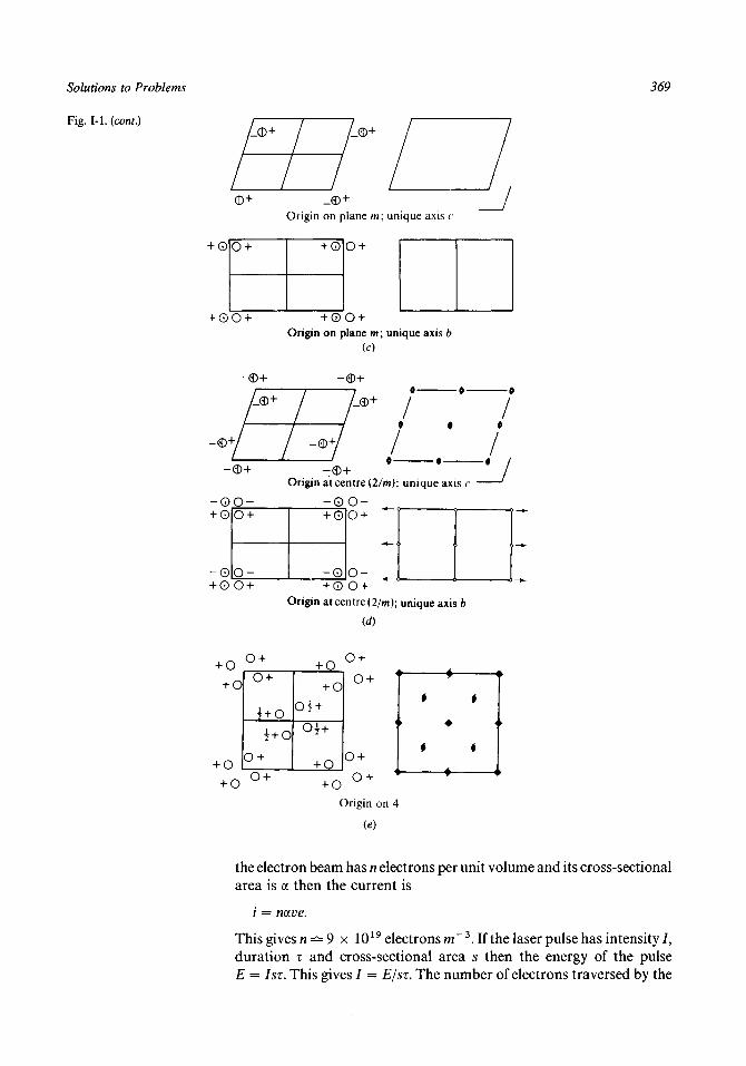
Solutions to Problems
Fig. 1-1. (cont.)
369
/_©+
0 + _0+Origin on plane m; unique axis c
- 0 +
- 0 O -
+ 0 O + +0O+Origin on plane m; unique axis b
(c)
-0-1- - ® +
_ / - 0 + / /
-W / /-0+ -0+
Origin at centre (2/m); unique axis c
-0O- -0O-+ 0
O O -+ 0 O+ + O O +
Origin at centre (2/m); unique axis b
id)
+ o+ o
+ O
+ Q0+
i+o
0 +
+ 001+
OH
+ 0
0 +
0 +
Origin on 4
the electron beam has n electrons per unit volume and its cross-sectionalarea is a then the current is
1 = nave.
This gives n 9 x 10¹⁹ electrons m 3. If the laser pulse has intensity /,duration x and cross-sectional area s then the energy of the pulseE = 1ST. This gives / = E/ST. The number of electrons traversed by the
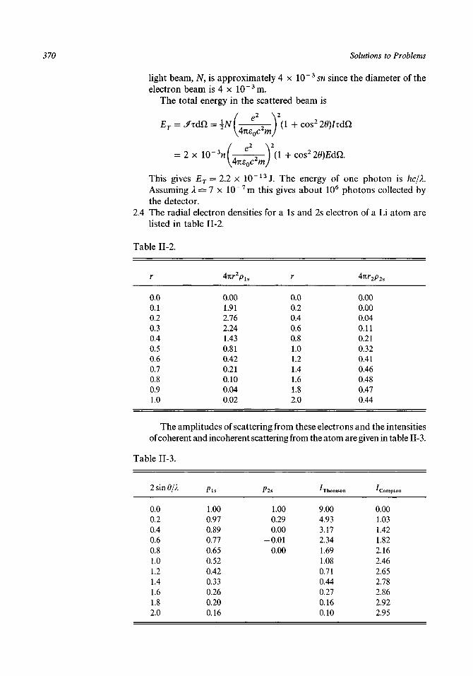
370 Solutions to Problems
light beam, JV, is approximately 4 x 10 ~3 sn since the diameter of theelectron beam is 4 x 10" 3m.
The total energy in the scattered beam is
/ e2 VET = ,/tdQ = iN[ =- (1 + cos2 20)/idQ
\4ns0c2mJ
( e2 V= 2 x 10"3n r-\ (1 + cos220)£dQ.
This gives ET = 2.2 x 10~13J. The energy of one photon is hc/LAssuming 2 ^ 7 x 10~7m this gives about 106 photons collected bythe detector.
2.4 The radial electron densities for a Is and 2s electron of a Li atom arelisted in table II-2.
Table II-2.
r
0.00.10.20.30.40.50.60.70.80.91.0
4nr2pls
0.001.912.762.241.430.810.420.210.100.040.02
r
0.00.20.40.60.81.01.21.41.61.82.0
4™2p2s
0.000.000.040.110.210.320.410.460.480.470.44
The amplitudes of scattering from these electrons and the intensitiesof coherent and incoherent scattering from the atom are given in table II-3.
Table II-3.
2sin0/;i
0.00.20.40.60.81.01.21.41.61.82.0
Pis
1.000.970.890.770.650.520.420.330.260.200.16
Pis
1.000.290.00
-0.010.00
^Thomson
9.004.933.172.341.691.080.710.440.270.160.10
''Compton
0.001.031.421.822.162.462.652.782.862.922.95

Solutions to Problems 371
Chapter 3
3.1 The values of K6 and K\ are given in table III-l.
Table III-l.
a*s
0.000.050.100.150.200.250.300.350.400.450.50
K6
6.005.173.080.68
-1.00-1.41-0.73
0.351.000.820.00
Kl
36.0026.769.470.461.002.000.530.121.000.670.00
a*s
0.500.550.600.650.700.750.800.850.900.951.00
K6
0.00-0.82-1.00-0.35
0.731.411.00
-0.68-3.08-5.17-6.00
0.000.671.000.120.532.001.000.469.47
26.7636.00
3.2 The orders of diffraction h and angles il/a are given in table III-2.
Table III-2.
h
0- 1- 2_ 3- 4
<Aa
30° 00'48° 14'62° 13'74° 34'86° 13'
h
-5- 6- 7- 8- 9
97° 42'109° 31'122° 16'137° 14'159° 04'
3.3 (i) a* = 0.231, fc* = 0.115, c* = 0.067 A" 1 , a* = p* = 90°, y* = 60°.(ii) V= 650A3, F* = 1.54 x 10" 3 A" 3 .
(iii) d321 = 1.20 A.(iv) 29= 80° 4'.
3.4 In table III-3 there is presented a selection of the output of STRUCFAC.If your solution agrees with this then the remainder will certainly becorrect.
3.5 In table III-4 there is presented the complete output of STRUCFAC.Notice the relationships between the structure factor magnitudes andphases of reflections with indices (h k 0) and (h k 0).
3.6 From V = abc(l — cos2 a — cos2 /? — cos2 y + 2 cosa cos /? cosy)* thevolume of the cell is 2.636 x 10~28m3. The mass of one molecule is1.3974 x 10~25 kg and for a density of 1.2 x 10³ kg m " 3 the number ofmolecules would be N = 2.26. The probable value of N is 2 and thisgives a density for the crystal of 1.061 x 10³kgm"3.
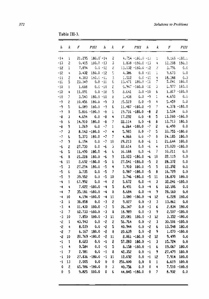
372 Solutions to Problems
Table III-3.
h
-14-13-12-12-11-11-10-10-10-9-9-9-8-8-8-7-7-7-6-6-6-6-5-5-5-4-4-4-4-3-3-3-3-2-2-2-2-1-1-1-1-100
k
I214
L.
5147/
253369369258
11369147
10147
10147
10147
101325
F
21.2950.4157.8943.4324.333
23.3491.688
11.0913.540
10.4566.0895.8164.694
14.9101.2698.1435.3736.194
27.73011.49021.2282.692
27.2943.735
39.95267.992
7.02235.1814.194
38.85811.43012.7337.850
43.9438.0396.167
20.7698.6230.5842.981
27.8362.005
65.9869.825
PHI
180.0'180.0
0.0.180.0
180.00.00.00.0
180.0180.0180.0
-180.00.0
180.00.0
-180.0180.0
0.00.0
180.0180.0
-180.0180.0
0.00.00.0
-180.0-180.0-180.0
0.0180.0
-180.0180.0
0.00.0
180.0-180.0
0.00.00.0
-180.00.0
-180.0160.0
h
-14-13
-12_ i ••
-11-10-10-10-9-9-8-8-8-7-7-7-7-6-6-6-5-5-5-5-4-4-4-4-3-3-3-3-2-2-2-2-1-1-1-1000
k
a
32c.•-'
I25
36147147
10369147
10253
11258
11258
11256
11036
F
4.7541.858
13.1324.3861.512
13.4710.9478.6411.438
15.51911.48719.71617.29222.1146.2645.9854.363
29.21322.61416.18815.02327.5417.9100.9873.7465.6728.4918.6643.0809.027
26.34716.98922.06156.76440.94420.6392.861
57.2638.158
42.35212.692
256.00040.75644.845
PHI
-idO.O-180.0-180.0
0.00.0
180.0-180.0
0.00.00.0
-180.0-180.0
0.00.0
-180.00.00.00.00.00.0
-180.0-180.0180.0
-180.0-180.0
0.00.00.0
-180.00.00.00.0
180.00.00.00.0
-180.0160.0
-180.00.00.00.00.0
-180.0
h
-13-13-12-11-11-11-10-10-9-9-9-8-6-6-7-7-7-6-6-6-6-5-5-5-5-4-4-4-4-3-3-3-3-2-2-2-2-1-1-1-1000
k
i
43-
4736*47258258147
10256
11369
12369
12369
12369
12147
F
•5.160IE.EOS3.7%9.673
18.3885.2416.9771.8174.6935.4594.3783.534
13.28013.7136.490
33.75524.16521.64419.03910.21122.11926.37212.39216.72918.67032.24112.10628.1606.228
13.8612.8342.5073.352
30.50113.5481.0709.499
15.72419.06727.4797.9146.6197.5108.932
PHI
130.00.00.00.0
180.0180.0
-180.00.00.0
-180.00.0
-180.0180.0
0.0-180.0180.0160.0
-180.00.00.00.00.00.0
180.0-160.0
0.00.0
180.00.0
180.0-180.0-180.0-180.0180.0
-180.00.00.0
160.0160.0180.0160.0
-180.00.0

Solutions to Problems 373
Table III-4.
h
-14-13-IE-11-11-10-10-9-9-8-8-7-7-6-6-5-5-5-4-4-3-3-2-2_p
-1-1000112223334455566
k
12
142536363625147362514736147250361472503614
F
8202371
121413,12.3,
16,16,22,26,16,3,
22,2,
11,7,
12,20.46.1.
11.20.2.0.
17.0.
32.10.8.
25.9.
36.10.7.
22.21.42.
.346
.798
.391
.637
.827
.396
.056
.173
.231
.908
.496
.864
.874
.051
.262
.741
.221
.623
.902
.417
.182
.126
.287,958,642,323,869000
,205000,605934745002941146889102562Oil964
14.1622.032
12.2.
094822
PHI
17614
-El96
-148149,-64,
-153,144,34.
155,-33.160.-57.
-175.-8.
171.23.
121.-41.-70.120.77.
126.-99.
-173.-52.
15.-30.80.
150.-107.-180.-113.
30.150.134.-55.11.
-54.180.
-132.-30.-63.
.8
.2
.1
.6
.4
.47
.9
.9
.6
.9
.6
.3
.6
.2,6.7,5,4,1,5,4,4,9,80,129910017121990607
-139.7
h
-14-13-IE-11- i l-10-9-9-8-8-7-7-7-6-6-5-5-4-4-4-3-3-2-2-1-1-1001112223344455566
k
E33Ec
3*41414736251473625147250361472503614725
F
81311E
IS18,17,12,7,
14,22,20.12.9.9.
30.9.
35.19.6.
10.16.17.10.70.11.12.41.0.
30.20.2.
46.1.
11.12.20.62.11.7.3.
22.2.
.490
.324
.713
.091
.392
.524
.533
.658
.344,641.071.837.379,729,732,278,933,422,099,762,644,045,364,499,661046394643000799323869287958642182126284902417741221623
26.05116. 262
PHI
-36,35.
-155,-149,-24.
-138.-37.-31.113.-8.
-177.-7.43.12.
117.-15.127.-3.
145.-86.
44.-17.
11.19.-9.
-43.-125.
.7
.0,6.7,0,4,1,4,8,6,9067472144341533
150.259.70.7.
-52.-102.126.80.
-70.-59.180.-58.-41.171.171.
0016925606147
-156.5-57.
4.68
h
-13-IE-IE-11-io-io
•~9
-9-8-8-7-7-6-6-6-5-5-4-4-3-3-3-2-2-1-10001112233344455666
k
1143
1
E5E5E5147362514736250361472503614725036
F
9.78618.70611.097S.866
19.4586.7636.1616.13b
4i.b77i0.32512.2997.357
IE.0942.622
18.30014.1622.032
22.562El .Oi l
36.14610.8897.102
25.0029.941
32.60510.934
256.0000.000
24.65570.66111.04612.39317.36410.49913.29910.64416.04535.42219.0996.762
30.2789.933
34.3229.7299.732
PHI
165.3-40.1
-139.8179.6
-154.3-40.3130.9E3.5
170.5-16.4
-162.3-117.8116.3
-139.720.047.4
-30.011.9
125.1-29.9134.2124.966.930.7
150.173.00.0
104.6-118.8170.5-43.354.711.4
-160.90.0
-135.6-17.3176.8145.193.6
-15.4-52.3
-180.0-167.4117.7

374 Solutions to Problems
Table III-4. {continued)
h
6776
a899
1010111112121314
k
7250362514141421
F
18.30012.2997.357
14.1873.908
16.4968.1816.136
19.4586.7637.6371.827
18.70611.09720.7988.346
PHI
-160.0-162.3
62.20.0
-145.4155.9130.9
-156.525.1
-40.3-83.4
-148.4139.9
-139.814.2-3.2
h
77788999
1010111112131314
k
0361403625252032
F
25.76616.86422.8747.344
14.64116.82213.17312.23112.39614.0562.091
18.39223.39122.03613.3248.490
PHI
180.0146.4160.3-66.6-8.80.0
26.1144.9149.4115.3
-149.8155.3-21.1180.0
-144.3-36.9
h
7778899
1010111112121314
k
147251403030310
F
22.07120.83712.37941.67710.32517.53312.65814.96818.52425.3878.8688.978
11.7139.786
10.056
PHI
2.4-7.9
-137.0170.5163.6142.6-31.1
-180.042.00.0
-0.4180.025.0
-14.10.0
Chapter 4
4.1 The output from SIMPl should be as follows:
h04
A '2 0 .- 0 .
( h )0 515
B(h)0. 000. 31
h15
A (h)0.27
- 0 . 02
B(h)6. 97
- 0 . 20
h2
A- 0
( h ). 76
B<- 1 .
h )17
h3
A (h)0. 62
B0
( h ). 17
4.2 The output from FOURl is as follows. This may be compared with thetable given in fig. 4.21.
THE COORDINATES ARE X/G
nO4a121620
19.9731. 4030. 119. 359. 2219. 97
n1591317
n/N WHERE N = 20
f (x)23. 3734. 4722. 457. 2510. 71
n26101418
f (x)26. 5737. 0916. 497. 0413. 26
n371 11519
f (x )29. 0936. OO12.528.0716.57
4.3 (i) F(S) =4n2s2
— fccos(2Tisa)] + k}.
(ii)

Solutions to Problems 375
4.4 -\>x c(x) = O
—i ^ x ^ I c(x) = — {1 + sin(27ix)}2TI
1 ^ , x sin(27ix)i ^ * -y- ^ * J2. /)/ Y |4 ^ - ^ 4 ^v^/ —
71
| < x < H c(x) = — {sin(27ix) - 1}.
. o o
4.5 (2u)-* exp{ - fa - 2)2}exp(27iix5)dx
- 2n2s2 + 47iis) exp{ - fa - 2 - 27iis)2}dxJ — oo
= exp( — 2n2s2 + 4TUS).
Fourier transform of g(x) = exp( — 2n2s2).Fourier transform of h(x) = exp(47tis).Hence Fourier transform of g(x)*h(x) = exp( — 2R2S2 + 47ii5).
-J 00 00 00
4.6 p{x,y,z) = - X X Z o)Wk2FllWcos(27cftx)cos(27cfcy)cos(27i/z)
where
coM/ = 8 if none of h, k, I is zero= 4 if one of h, k, I is zero= 2 if two of h, k, I are zero= 1 for h = k = I = 0.
The range of summation is 0 — \ for x, y and z.4.7 Part of the projected density is shown in fig. 4.20. If this region is found
in the map then the map is almost certainly correct.
Chapter 5
5.1 This problem can be solved graphically. It will be found that if areciprocal-lattice net is rotated over a diametral section of the sphere ofreflection then one must rotate the net 54° between the (907) and (702)reflections.
5.2 (a) 6.3, 13.5, 24.0 mm.(b) The layer lines indicate a = 9.91, 9.97, 10.01 A, respectively.
5.3 Fig. V-l shows the fit of the reciprocal lattice on to the arcs within theallowed regions of reciprocal space. The reflections which are observedare indicated. The reflections too weak to be observed have indices(420), (340) and (410).
5.4 Fig. V-2 shows two reciprocal-lattice points, (hk) inside circle and (h'k1)outside.
For a point inside the circle, the angle through which the crystalmust be rotated is ij/ = (n/2) — 6 + (j) and the intersection will be withthe lower section of the circle.

376 Solutions to Problems
For a point outside the circle, the intersection can be with either theupper section or the lower section - the angle of rotation in the twocases being, respectively,
= ^ + 0 - 0' or 0 + 0 - 1
and
A reflection will be produced if 0 ^ \j/ ^ 180°. With the y coordinate onthe upper section taken as positive and on the lower section taken asnegative the (x,y) coordinates on the film are as listed in table V-1.
Table
h
11111
TTTTTTTTTT
V-1.
k
165432T01234567
x(mm)
61687480856164267727169666155
y(mm) /
65 15140312316959162331405165
i k
L 1L 6I 5L 4I 3L 2L 1L 0t TL 2L 3L 4[ 5L 6[ 7
x(mm)
35292521191823537688510162229
y(mm)
-65-51-40-31-23-16-9-5-9-16-23-31-40-51-65
5.5 From equation (5.24) the critical wavelength in angstroms is given by
_ 18.64
'"BE2
where B is in tesla and E in GeV. Inserting the given values Xc = 1.883 A.From equation (5.23) the vertical divergence of the beam is given by
me2
E
where E is the energy of the electron beam. This gives
?JL 9.108 x 10"3 1 x ( 3 x 10⁸)2
3 x 109 x 1.602 x 10~19 = 1.706 x 10 " 4 radians
= 35".

Solutions to Problems 377
Fig. V-l.Diagram for solution5.3.
(100)
(100)
,(460)
(440)
Fig. V-2.Diagram for solution5.4.
Incidentbeam
/ ^ ^
/ Direction
/ o f
/ rotation
1 ^
b
1(h'k')
Aa
Section ofsphere ofreflection
5.6 Let the intensities of the (231) and (462) reflections be lx and /2,respectively. The (462) reflection corresponds to the shorter wavelengthso that
/ ! + / 2 = 262and
i + 0.3/2 = 106.

378 Solutions to Problems
Solving the simultaneous equations gives
I, = 91.33; I2 = 170.67.
Chapter 6
6.1 3.56 x 108.6.2 4720 m" 1 .6.3 The reflecting planes make an angle 45° with the cell edges and
6 = 21.3° for the (240) reflection. The crystal can be divided into tenregions as shown in fig. VI-1. The details of the calculation are given intable VI-1.
Table VI-1.
Point x (mm) x' (mm) x + x' (mm) • x') exp{ - t x')}
123456789
10
0.820.820.820.820.500.270.270.270.270.27
0.220.620.620.620.620.220.661.091.531.85
1.041.441.441.441.120.490.931.361.802.12
5.207.207.207.205.602.454.656.809.00
10.60
0.005 520.000750.000750.000750.003 700.086300.009 560.001110.000120.00002
0.108 58
A = 0.108 58 = 0.0109.
Fig. VI-1.Division of the crystalfor the absorptioncalculation.
6\
\ \
\ \ \ \ \ \
Direction ofreflecting
plane
i I I 1 i i i i1 mm

Solutions to Problems 379
6.4 In table VI-2 there is presented a selection of the output of STRUCFAC.If your solution agrees with this then the remainder will certainly becorrect. Compare this solution with that of Problem 3.4 and notice thatthe effect of the temperature factor becomes more pronounced forreflections with higher Bragg angles.
Table
h
-14-13-12-12-11-11-10-10-10-9-9-9-8-8-8-7-7-7-6-6-6-6-5-5-5-4-4-4-4-3-3-3-3-2-2-2-2-1-1-1-1-100
VI-2.
k
l21425147258369369258
11369147
10147
10147
10147
101325
F
6.7450.1453.3701.1912.0288.4800.9285.0411.1686.1272.8471.9072.8727.0310.4055.4662.8032.206
21.2837.2169.5820.767
21.3232.30617.11861.0125.472
20.9201.672
36.3719.3698.0293.346
42.4226.8524.0789.3598.4900.5122.04413.1140.57064.1148.207
PHI
180.0180.0
0.0180.0180.0
0.00.00.0
180.0180.0180.0-180.0
0.0180.0
0.0-180.0180.0
0.00.0
180.0180.0-180.0180.0
0.00.00.0
-180.0-180.0-180.0
0.0180.0-180.0180.0
0.00.0
180.0-180.0
0.00.00.0
-180.00.0
-180.0180.0
h
-14-13-12-12-11-11-10-10-10- 9-9-8-8-8-7-7-7-7-6-6-6-5-5-5-5-4-4-4-4-3-3-3-3-2-2-2-2-1-1-1-1000
k
23253625836147147
10369147
10258
11258
11258
11258
11036
F
1.4180.5975.3081.3800.6544.3850.4963.5810.4158.5574.84213.3539.8409.2904.6293.7482.2698.902
16.4699.2385.902
23.4275.7960.5471.3814.9266.1354.5851.0448.201
20.07510.6618.025
53.33432.53312.1841.102
55.0416.684
25.9955.127
256.00038.20134.612
PHI
-180.0-180.0-180.0
0.00.0
180.0-180.0
0.00.00.0
-180.0-180.0
0.00.0
-180.00.00.00.00.00.0
-180.0-180.0180.0-180.0-180.0
0.00.00.0
-180.00.00.00.0
180.00.00.00.0
-180.0180.0-180.0
0.00.00.00.0
-180.0
h
-13-13-12-11-11-11-10-10-9-9-9-8-8-8-7-7-7-6-6-6-6-5-5-5-5-4-4-4-4-3-3-3-3-2-2-2-2-1-1-1-1000
k
l4314736147258258147
10258
11369
12369
12369
12369
12147
F
3 .3873 .6401.4324.7137.3441.5073.4280.6772.8802.7921.6392.2916.9295.0584.60419.4319.925
17.25712.9685.2207.455
23.2968.3948.2135.898
26.7177.992
13.0111.769
12 .0471.9781.2351.024
27.4949.8910.5563.08514.53514.39314.8832.7026.5726.6946.278
PHI
-180.0180.0
0.00.00.0
180.0180.0-180.0
0.00.0
-180.00.0
-180.0180.0
0.0-180.0180.0180.0-180.0
0.00.00.00.00.0
180.0-180.0
0.00.0
180.00.0
180.0-180.0-180.0-180.0180.0-180.0
0.00.0
180.0180.0180.0180.0-180.0
0.0

380 Solutions to Problems
Table VI-3.
6.5 Part of the output of STRUCFAC is shown in table VI-3. Neighbouringpairs of structure factors form Friedel pairs (hkO) and (hkO). Withoutanomalous scattering these would have equal amplitudes and oppositephases. Note the breakdown of this condition.
PHI PHI PHI
12111010-99
-98
-88
-77
-77
-66
-66
-55
-55
-54-44-44-33
-33
-32
-22
-22
-11
-11
_ -\10000001
1-11
-21
-24-13
-41
-24
-51
-24-51
-24
-57
-13
-46-72
-35
-68
-13
-46-71
-24-57
-81
-24
-57-80
13.92113.75413.48015.66023.47316.33411.27827.56421.77716.50820.58218.99920.55314.19320.87220.90416.94515.50526.21226.50421.92014.70911.88920.93722.60626.11614.08315.32021.85824.70528.65719.55215.04529.03424.69016.99622.45913.81518.17929.40625.29716.77614.98713.07937.80832.51420.09123.39320.01314.10447.659
-81.0-124.5
23.7-86.3
-112.949.5
145.4-82.5-90.4-11.7-57.3-43.7
-131.341.7
-175.287.292.5
-175.640.0
-136.3-33.3-57.0
-122.3109.394 .7
-166.318.2
-89.8-151.5
48.6127.2123.659.87.5
174.183 .094.6
-171.3-123.8
37.9140.2134.863.0
-119.9125.7
-175.6-3.4
-82.9-71.8-4.7
-169.7
12-1110
-109-99
-88
-87
-77
-76
-66
-65
-55
-55
-44-44-33-33-33
-22
-22-21
-11
-110000000
-1
-12
-13
-13
-42
-35
-13
-46
-13
-46
-13
-46
-72-35-61-24-57-82-35-68
-13
-46
-70
-13-46-790
13.76713.52412.59411.99722.53818.53811.12817.72221.99111.54521.39617.08220.57310.67020.83415.85317.07013.22826.62521.10021.52114.16611.60329.00922.55525.81113.45923.09222.85916.85329.19615.93314.57619.53425.15918.11822.41616.81217.84318.82025.20119.90114.35471.05536.18426.74020.47123.01119.29912.52449.379
93.0-125.4-11.4
-164.8119.863.1
-130.5-172.598.093.265.0
124.7139.443.9
-176.78.5
-82.6-78.4-33.7
-125.041.0141.1136.5-7.6
-87.3-71.0-6.3
146.7158.527.3
-121.5-43.8-48.6100.1-167.5-22.0-87.1-90.6133.046.9
-133.6-42.5-51.9
1.2-121.9-69.011.6
-175.680.0
105.2172.5
-1111
-1010-99-88
-88
-77
-77
-66
-66
-55
-55
-44
-44-43-33-33
-22
-22
-22
-11
-11
-100000001
1-22
-32
-31
-24-52
-35
-62
-35
-62
-35
-61
-24
-57
-13
-46
-71
-24-57
-82-35-6802-35-68-91
13.529 136.713.352 137.915.743 96.911.577 178.816.367 -39.217.849 -54.127.336 88.617.582 -178.017.338 21.211.751 -78.819.155 52.417.837 -115.414.651 -30.311.116 -28.721.248 -79.315.691 2.115.554 -173.612.962 91.226.728 142.520.793 133.015.582 67.614.159 -129.220.160 -101.529.536 13.225.581 172.625.014 77.415.587 100.622.681 -139.524.695 -41.817.956 -18.420.332 -115.516.137 54.228.797 -1.819.239 -91.517.592 -73.519.402 30.013.682 -176.517.095 100.529.910 -32.318.951 -38.017.041 -124.919.988 50.912.636 132.871.055 1.232.420 -179.325.838 75.023.215 90.122.974 -177.114.634 16.112.093 -91.749.924 -36.9

Solutions to Problems 381
Chapter 7
7.1 (a) Fhkl = 0 for h + k + I = In + 1.(b) Fhol = 0 for h + I = In + 1.(c) For 3l axis along ft, JFOkO = 0 for h ^ 3n.
7.2 (a) P21/c. (ft) Pna2v
7.3 For each projection the reflections are taken in groups of twenty andthe intensities are compared with the average within the group. Thisgives the results shown in table VII-1.
This indicates that the (hOl) projection is centrosymmetric and the(0/c/) projection is non-centrosymmetric.
Table VII-1.
(hOl) data (0/c/) dataN(Z) N(Z)
0.10.20.30.40.50.60.70.80.91.0
0.200.330.400.470.500.600.630.650.680.70
0.130.200.280.350.400.430.480.500.560.62
7.4 The first part of the output is given as table VII-2. If your results agreewith this then you may assume that the remainder is correct.
Table VII-2.
a = 0.423E-01VALUES OF E
H- 1 4- 1 4- 1 4- 1 3- 1 3- 1 3- 1 2- 1 2- 1 2- 1 1- 1 1- 1 1- 1 1- 1 0- 1 0- 1 0- 1 0
- 9- 9- 9
K147258258147
10258
1 1369
b = 0
E1 .2431 .0280 . 8 0 30 . 0 3 30 .1180 . 7 9 30 .8120 .3670 .9880 . 5 1 11 .2190 . 4 3 10 . 0 0 30 .0380 .5980 .0640 .8230 .9980 . 8 5 10 .837
.701E-02
H- 1 4- 1 4- 1 4- 1 3- 1 3- 1 3- 1 2- 1 2- 1 2- 1 1- 1 1- 1 1- 1 1- 1 0- 1 0- 1 0
- 9- 9- 9- 9
c = 0
K258369369258
1 1369147
10
.648E-02
E0 .3030 .3230 .3130 .1242 . 3 6 71 .0990 .2740 .4940 .0350 .2591.7170 .0730 . 2 2 10 .3900 . 1 5 10 .6750 .2380 . 3 2 10 .3650 .506
H- 1 4- 1 4- 1 3- 1 3- 1 3- 1 2- 1 2- 1 2- 1 2- IX- 1 1- 1 1- 1 0- 1 0- 1 0- 1 0
- 9- 9- 9- 9
K36147147
10369147
10258
1 1
E1 .1231 .7300 .5230 .8450 .4580 .4390 .2340 .6520 .5050 .1401 . 0 1 10 . 7 6 00 . 0 7 80 .7660 .2721 .8100 . 5 6 30 .4140 . 5 1 10 .105

382 Solutions to Problems
Chapter 8
8.1 Let the coordinates of Cu atom be x, y, and of Cl atom be x', / . Atomicno. of Cu = 29 and of Cl = 17. Thus there are the following peaks:
single weight Cu—Cu at 2x,2y of weight 841single weight Cl—Cl at 2x', 2 / of weight 289double weight Cu—Cl at x + x',y + / of weight 986double weight Cu—Cl at x - x\y — y' of weight 986.
Examination of the Patterson function gives
x = 0.074 y = 0.193x' = 0.249 / = 0.146.
Superposition methods can be used to locate the two other atoms. Theyare at
x = 0.05
and
x = 0.27
y = 0.60
y = 0.67
for
for
N
C.
Check that these give vectors with the other atoms which are consistentwith the Patterson.
8.2 The Patterson map is shown in fig. VIII-1 and it will be seen that thereare two major peaks other than the origin peak. Peak B gives the S—Svector (2x, 2y) at (0.3,0.6). Where there are alternative peaks it may benecessary to try both to see which one gives a plausible solution. Thefinal Sim map is shown in fig. VIII-2.
8.3 The difference Patterson map is shown in fig. VIII-3 and clearly showsthe S—S (or O—O) vector.
8.4 The vectors between the sulphur atoms are at ±(0.188,0.100),±(0.438,0.700) and ±(0.250,0.600). These can be clearly seen in thedifference Patterson map which is given in fig. VIII-4. The final mapgiving the carbon positions is shown in fig. VIII-5.
8.5 The anomalous-difference Patterson map is shown in fig. VIII-6. Thehighest non-origin peak corresponds to the S—S vector.
8.6 The Ps-function map is given in fig. VIII-7. It would be difficult tointerpret it completely for the positions of the light atoms but severalcould be approximately located. The two atoms not on peaks areapproximately centrosymmetrically arranged about the mercury atomso their densities partially cancel each other.
8.7 The complete set of signs for this projection is given in table VIII-1.Other solutions are possible which represent transformation to
other centres of symmetry as origin. If the reflections are divided intofour groups (k even, / even); (k even, / odd); (k odd, / even); and (k odd, /odd), then multiplying complete groups by the signs given belowcorresponds to transforming to the three other origins:
(even, even) + + +(odd, even) — + —(even, odd) + — —(odd, odd) +
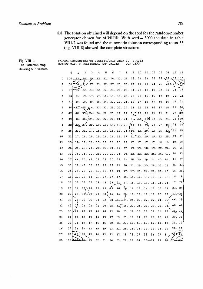
Solutions to Problems 383
8.8 The solution obtained will depend on the seed for the random-numbergenerator chosen for MINDIR. With seed = 3000 the data in tableVIII-2 was found and the automatic solution corresponding to set 33(fig. VIII-8) showed the complete structure.
Fig. VIII-1.The Patterson mapshowing S-S vectors.
FACTOR CONVERTING TO DENSITY/UNIT AREA IS 3.4333OUTPUT WITH Y HORIZONTAL AND ORIGIN TOP LEFT
Q
1
2
3
4
5
6
7
8
9
10
11
12
13
14
15
16
17
18
19
20
21
22
23
24
25
26
27
28
0
100
66
27
22
21
30
42
39
28
25
21
19
26
33
37
33
26
19
21
25
28
39
42
30
21
22
27
66
100
1
21.
20.
48.
46.
23.
17.
18.
26.
36.
44.
38.
26.
19.
25.
31.
28.
28.
2;7.
/L.19.
21.
24.
-46."
2
J>19
18
•^5
N
3
/ 27.
. 21.
. 17.
. 20.
A4-35 N 24.
\
36
21
16
17
25
38
51
43
26
19.
25.
3V
26.
21.
18.
16.
19.
23.
/24.
20.
17.
16.
16.
21.
32.
42.
36.
22.
18.
22.
^26.
.'27.
25.
21.
17.
15.
17.
22.
25.
4
31.
22 .
17.
25.
32.
26.
22.
19.
15 .
15.
15.
20.
28.
31.
25.
19.
17.
19.
22.
23.
23.
21.
16.
14.
16.
19.
24.
5
32.
22 .
18.
26.
33.
28.
22.
19.
14.
14.
17.
22.
30.
29.
22.
18.
17.
19.
29.
22.
20.
18.
15.
15 .
19.
22.
6
27.
21.
17.
21.
25.
25.
22.
19.
15.
14 .
16.
21.
29.
30.
22.
19.
17.
23.y
,43.
44.
2"8._
25.
22.
17.
20.
23.
22.
7
23
?1
18
19
22.
22.
21.
19.
16.
15.
15.
17.
23.
25.
22.
19.
17.
21.
40.
44.
3L.31'""
28.
19.
25.
31.
27.
8
28.
28.
23.
21.
27.
28.
24.
28.
24.
17.
15.
17.
20.
22.
20.
17.
15.
17.
2k.t/
27.
21.
23.
28.
28.
9
27
31
25.
19.
28.
3l:/ '44.(\40.
10
22.
23 .
20.
17.
22.
-28^
44.
43.
21^23^
17.
19.
22.
25.
23.
17.
15.
15.
16.
19.
21.
22.
22.
19.
18.
21.
23.
17.
19.
22.
30.
29.
21.
16.
14.
15.
19.
22.
25.
25.
21.
17.
21.
27.
11
22.
19 .
15.
15.
18.
20.
2B
30»y.19.
17 .
18.
22.
29.
30.
22.
17.
14.
14.
19.
22.
28.
33.
26.
18.
22.
32.
12
24.
1 9
16.
14.
16.
21.
23.
23.
22.
19.
17.
19.
25.
31.
28.
20.
15.
15.
15.
19.
22.
26.
32.
25.
17 .
22.
31.
13
25.
22 .
17 .
15.
17.
21.
25.
27.
26.
22.
18.
22 .
36.
42.
32.
21.
16.
16.
17.
20.
24.
24.
24.
20.
17.
21.
27.
14 15
28X46
23 .
19.
16.
18.
21.
26.
3 2 O
25.
19.
26.
43.
51.
38.
25.
17.
16.
21.
27.
36'.
351.
25.
18.
19.
22.
31.^s
24
21
19
22
27
28
25
19
26
38
44
36
26
18
17
23
J2
46
48
20
21
26
I
16
i no
S ^
2?
. 22
. 21
• 30<r
. /42•
1139\
. 25
. 21
. 19
. 26
. 33
. 37
. 33
. 26
. 19
. 21
. 25
.-28
. 39
. 42
. 21
. 22
. 27
<66
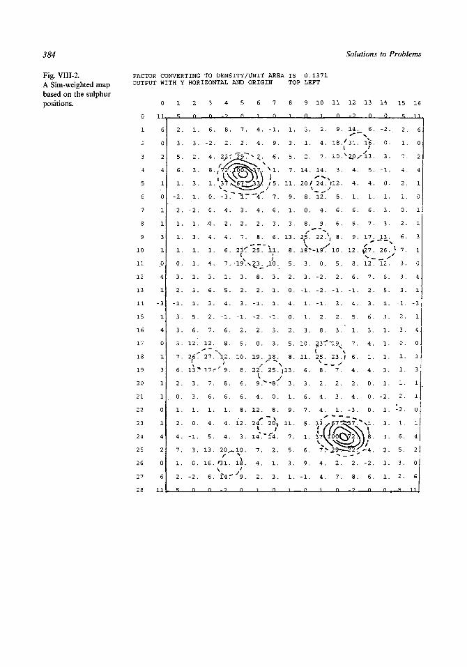
384 Solutions to Problems
Fig. VIII-2.A Sim-weighted mapbased on the sulphurpositions.
FACTOR CONVERTING TO DENSITY/UNIT AREA IS 0.1371OUTPUT WITH Y HORIZONTAL AND ORIGIN TOP LEFT
0
1
2
3
4
5
6
7
8
9
10
11
12
13
14
15
16
17
18
19
20
21
22
23
24
25
26
27
28
0
11
6
0
2
4
1
0
1
1.
3
1
0
4
1
-3
1
4
0
1
3
1
1
0
1
4
2
0
6
11
10 11 12
n
13 14
n. n.
15 16
2
3.
5.
6.
1.
-2
2.
1.
1.
1.
0.
3.
2
-1
3.
3
3 .
7.
6.
2.
o.
1.
2.
4 .
7.
1.
2.
q
1
3.
2.
3.
3.
1
-2.
1.
3.
1.
1.
1.
3 .
1
5.
6
12 .
¥•13:*
3 .
3 .
1.
0.
-1.
3.
0.
-2.
n
-2.
-4.
8.
1.
o
0.
0.
4.
1.
4 .
3.
6
2.
7
12.
8
2
2?
(12
-•3,
4
2
4
6
7
1
s
4
-1
8
*27.\.2
17r
7.
6.
1.
4.
5.
13.
16.
6.
n
' 9
8
6
1
4
4
20
Ol
*4
_ 9
7
. 2
,-29
.v67
. 3
. 2
. 7
I
. 3
2
3
. -1
2
. 5
. 10
. 8
. 6
. 6
. 8
. 12
. 3
.— 10
• ^
n
4
4.
\ ^
^ v
4
4.
. 2.
. 8.
< *25.
A 2 3 .
. 8.
2 .
-1
. -2.
-2
. 0.
. 19.
. 9.s
4.
. 12.
. 24"I
. 14\"
7 .
4.
. 2.
i
-1
9
6
^1
7
6
3
6
11
yo3
1
1
-1
3
•* •>
25
•-8
0
8
/
2
1
3
n
1
. 3.
. 5.
7.
. 11.
9
1.
. 3.
. 13.
. 8.
. 5.
. 2.
0.
4
. 0.
2
. 5.
. 8.
. ,13.
f 3.
1.
. 9.
\ 11-
7.
. 5.
. 3.
. 1.
i
3 .
1.
2.
14.
20/
8
0.
8.
13.
3.
-1.
1
1.
3
10.
11.
6.
3.
6.
7.
5.
1.
6.
9.
-1.
n
2
4
7
14
24
9
. 18
. 10
. 3
j
12 8
4
9
22
-19-
0
-2
-2
-1
2
8
I25
8
2
4
4
)!iV74
4
. 6
. 6
* J
''lO
. 5
. 2
. -1
3
. 2
3
-19
. 23
7
2
. 3
. 1
. 2
. 7
n
/
\
\.1
1 4
31.
2,0,
4.
4.
1
6.
8.
9.
12.
8.
6.
-1
4
5.
1
7.
6.
4 .
2 .
4.
-3.
2.
8.
-?
l).
^ 1 3 .
5.
4.
1
6.
7.
17.
127.
12*7
7.
2
3
6.
3
4.
1.
4.
0.
0.
0.
"Nl.
I-2.
6.
n
-2 .
0.
3.
-1.
0.
1.
3.
3.
26.
"12.
6.
5.
1
3.
1
1.
1.
3.
1.
-2.
1.
ro
ro
CN
3.
1.
n
2 .
1.
7 .
4 .
2 .
1.
0 .
2.
6.
t 7.
3.
3 .
3
-1
2 .
3 .
0.
1.
1.
1.
2 .
-2.
1.
6.
5.
3.
2.
6
0
2
4
1
0
1
1
3
1
0
4
1
-3
1
4
0,
1.
3
1
1
0
1
4,
2]
0
6
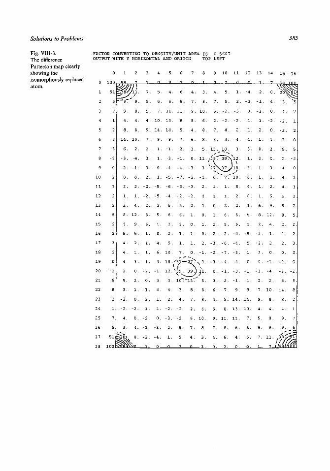
Solutions to Problems 385
Fig. VIII-3.The differencePatterson map clearlyshowing theisomorphously replacedatom.
FACTOR CONVERTING TO DENSITY/UNIT AREA IS 0.5607OUTPUT WITH Y HORIZONTAL AND ORIGIN TOP LEFT
0
1
2
3
4
5
6
7
8
9
10
11
12
13
14
15
16
17
18
19
20
21
22
23
24
25
26
27
28
0
100
51
5
7
1
2
8
5
-2
0
2
3
2
2
5
2
2
3
2
0
-2
5
8
2
1
7
5
51
100
1
—97
9.
4 .
8.
14.
6.
-3.
-2.
0.
2
1.
2
8.
5.
5.
4.
4.
4 .
2
5.
3.
-2.
-2.
4
3.
$20%
2
7)/*>A/." 9.
8.
4.
8.
10.
2.
-4.
-1.
0
?
1.
4 .
12.
9.
5.
2 .
1.
3.
0
2.
1.
0.
-2.
0
4.
o
3
1
7.
9.
5.
4.
9.
7.
2.
-3.
0.
2
-2 .
-2.
2 .
8.
6.
1.
1.
1.
1.
-2 .
0.
1.
2.
1.
-2 .
-1.
-2 .
1
4
n
5.
6.
7.
10.
14.
9.
1.
-1.
0.
1.
-5.
-5.
2 .
5.
1.
0.
4.
6.
3.
-1.
3.
4.
1.
1.
0.
-3.
-4 .
n
5
n
4
6
11
13
14
9
-1
-3
-4
-S
-6
-4
8
2
2
5
10
18
1 ?
3
4
2
-2
_^
2
1
6
. 6.
. 8.
. 11.
. 8.
. 5.
. 7.
. 2.
. -1.
. -4 .
-7
. -6 .
. -2.
5
. 6.
. 2.
. 1.
. 1.
7.
(f. V39.
. 3.
. 4.
. -2.
. -2 .
. 5.
5.
7
n
4.
7.
9.
5 .
4 .
6.
3.
0.
-3 .
-?
-2 .
?
1.
0 .
1.
1.
0.
2^>
13".
8.
7.
2.
7.
4
n
8
1
3.
8.
10.
6.
8.
8.
5.
11.
3.
-1
2
0.
1
0.
1.
0.
2.
-1.
N 3 .
1V1
5 .
8.
8.
6.
10
8.
3
1
9
n
4 .
7 .
6.
2 .
7.
8.
13.
fto
1
1.
o
1.
2.
-2.
-3.
-2.
-3 .
o
3 .
6.
4.
5.
9
7 .
4
o
10
5.
5.
-2.
-2.
4 .
3 .
10.
T?>>
" 7*"
1.
1.
2
6 .
5.
-2.
-6.
-7 .
-4.
-1
2 .
7.
5.
8.
11.
8.
11
n
I.
2.
-3.
-2.
2.
4.
3.
^12.
)l8.
10
S
2 .
?
8.
5 .
-4 .
-6.
-5.
-4 .
_^
-1.
9.
14 .
13.
11.
6.
4 .
0
12
n
-4.
-3.
0.
1.
1.
4 .
3.
-1.
3 .
6
4 .
0 .
1
5 .
2.
-5.
-5.
1.
0 .
-1.
1.
9.
14.
10.
7.
6.
5.
0
13
1
-2.
-1.
-2.
1.
2.
1.
0.
-2.
1.
1
1.
1 .
6
8.
2.
-2.
-2.
2 .
0.
-3 .
2.
7 .
9.
4 .
5 .
9.
7.
1
14
7
0 .
4.
0.
-2 .
0.
1.
2.
0.
3 .
1
?
5.
9
12 .
4.
1.
2.
0.
-1.
-4 .
2.
10.
8.
4 .
8
9.
11
7
15
\ ^
3.
4 .
-2.
-2.
3.
5.
2 .
4 .
4 .
4 .
5.
5
8.
2 .
1.
2 .
0.
-2.
-3 .
6.
14.
8.
4 .
9 .
9.
3*8^
16
innit**5
7
1
2
8
5
-2
0
2
3
2.
2 .
5.
2 .
2 .
3.
2.
0.
-2 ,
5.
8.
2,
1.
7 .
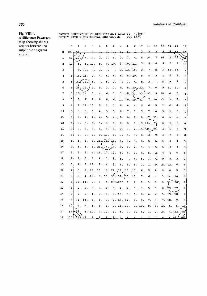
386 Solutions to Problems
Fig. VIII-4.A difference Pattersonmap showing the sixvectors between thesulphur (or oxygen)atoms.
FACTOR CONVERTING TO DENSITY/UNIT AREA ISOUTPUT WITH Y HORIZONTAL AND ORIGIN TOP
o
1
2
3
4
5
6
7
8
9
10
1 1
12
13
14
15
16
17
18
19
20
2 1
22
23
24
25
26
27
28
0
1 0 0
59
10
7
8
6
6
3
7
6
1
5
4
5
8
5
4
5
1
6
7
3
6
6
8
7
10
59
100
1
M
9 .
1 8 .
21/'t
1 0 .
5 .
6 .
3 .
5 .
3 .
3 .
9 .
8 .
6 .
5 .
2 .
4 .
6 .
6 .
1 1 .
9 .
9 .
1 1 .
4 .
"VV
2
U.5 .
1 0 .
1 5 .
"2*9 "
3 1 .
1 4 .
8 .
12 .
8 .
4 .
3 .
3 .
7 .
6 .
5 .
5 .
6 .
6 .
3 .
4 .
1 1 .
9.
6.
1 1 .
7 .
3 .
3
q
1 0 .
1 2 .
7 .
3 .
* g
/ 9 .
3 .
9 .
1 5 .
9 .
4 .
6 .
5 .
3 .
4 .
6 .
4 .
6 .
1 2 .
1 3 .
1 0 .
9 .
5 .
1 .
3 .
8 .
1 0 .
9
4
^
2
5
3
4
7
5
4
8
9
4
2
5
6
9
2 1
2 3
1 1
6
9
1 0
9
6
7
8
5
4
7
5
-\
. 3
. 8
7
. 6
5
. 3
. 6
. 5
1
. 3
. 5
4
. 5
. 13
•/ 31
I\ 3 4
. 17
7
. 6
7
. 10
7
. 2
. 6
7
. 8
. 10
6
. 6.
. 10.
7 .
. 6.
3
. 2 .
. 7.
. 6.
. 3 .
. 5 .
4 .
4 .
. 6.
. 6.
^ 1 5 .
. 19 .
. 10.
. 5 .
. 9.
. 2 1 .
. 3 3 .
. 23>
. 5 .
. 5 .
. 8 .
7 .
. 6 .
7
1
3 .
3 .
2 .
6 .
7 .
8 .
1 2 .
1 1 .
8 .
6 .
0 .
2 .
7 .
3 .
4 .
9 .
8 .
5 .
6 .
^19^.
3 2 .
-20 1
4 .
1 0 .
1 6 .
1 1 .
4 .
1
8
6
7 .
1 0 .
1 2 .
8 .
2 .
8 .
1 5 .
1 0 .
6 .
7 .
6 .
6 .
7 .
5 .
7 .
6 .
6 .
7 .
6 .
1 0 .
\ s .
8 .
2 .
8 .
1 2 .
1 0 .
7 .
4 . 5 5 5 7LEFT
9
4 .
1 1 .
1 6 .
1 0 .
4
3 2 .
1 9 .
6 .
5 .
8 .
9 .
4 .
3 .
7 .
2 .
0 .
6 .
8 .
1 1 .
12 .
8 .
7 .
6 .
2 .
3 .
3 .
1 ,
10
?
6
7
8
5
5
- 2 3 >
3 3
9
5
10
19
1 5
6
6
4
4
5
3
6
7
2
3
6
7
10
6
1 1
3
. 1 0 .
. 8 .
7 .
. 6 .
2 .
7 .
Vo./
7 .. 6 .
7 .
. 1 7 .
. / 3 4 .
. N31.
. 1 3 .
. 5 .
4 .
. 5 .
. 3 .
1 .
5 .
6 .
. 3 .
. 5 .
. 6 .
7 .
. 8 .
. 3 .
12
7 .
4 .
5 .
8 .
7 .
6 .
9 .
1 0 .
9 .
6 .
1 1 .
^ 2 1 .
9 .
6 .
5 .
2 .
4 .
9 .
8 .
4 .
5 .
7 .
4 .
3 .
5 .
Lo
to
1 3
9 .
1 0 .
8.
3 .
1 .
5
9 .
1 0 .
1 3 .
12 .
6 .
4 .
6 .
4 .
3 .
5 .
6 .
4 .
9 .
1 5 .
9 .
3 .
9 .
8 .
3 .
7 .
1 2 .
1 0 .
1 4
3
7
1 1
6 .
9
1 1 .
4 .
3 .
6 .
6 .
5 .
5 .
6 .
7 .
3 .
3 .
4 .
8 .
1 2 .
8 .
1 4 .
L1 5 .
1 0 .
5 .
4 .
15 '
4 .
1 1 .
9 .
9 .
1 1 .
6 .
6 .
4 .
2 .
5 .
6 .
8 .
9 .
3 .
3 .
5 .
3 .
6 .
5 .
1 0 .
76>
2 7 . /S
1 8 .
9 .
5 .
1 6
sa.
10
7
8
6
3
7
6
1
5
4
5
8
5
4
5
1
6
7
3
6
6
8
7
10
i s i f i n n

Solutions to Problems 387
Fig. VIII-5.Map showing thecarbon atoms withphases from sulphuratom positions asdeduced from fig.VIII-4.
FACTOR CONVERTING TO DENSITY/UNIT AREA IS 0.0392OUTPUT WITH Y HORIZONTAL AND ORIGIN TOP LEFT
o1
2
3
4
5
6
7
8
9
10
11
12
13
14
15
16
17
18
19
20
21
22
23
24
25
26
27
28
9
11
2
-3
3
4
-2
-7
0
21
34
26
16
16
16
10 11 12 13 14 15 16
-5
21
37.
24.
19.
15.
9.
16.
16.
4.
2.
3.
2.
4.
2.
-2.
2.
4.
8.
8.
9.
16.
12.
13.
31.
32.
9.
-5.
7.
•\->
13.
12.
12.
9.
13.
34.
34.
13.
8.
7.
-3.
-7.
-4.
5.
8.
6.
3.
-5.
-7.
6.
13 .
22.
45.
48.
26.
14.
12.
11
6.
10.
10.
8.
11.
22.
18.
7.
10.
10.
-4.
-12.
-11.
-13.
-1.
0.
7.
9.
0.
-4.
-1.
8.
25.
28.
16.
7.
2.
n
21.
9.
7.
21.
22.
4.
-9.
-2.
6.
-3.
-13.
-9.
-5.
-22.
-1.
3.
8.
11.
6.
6.
10.
5.
4.
13.
15.
2.
-1.
1 i
9.
-3.
-6.
15.
28.
13.
1.
9.
14.
1.
-10.
-7.
-3.
-11.
-9.
-1.
14.
17.
2.
-4.
12.
19.
9.
10.
18.
10.
0.
-7.
-3.
-1.
0.
11.
13.
4.
2.
6.
14.
23.
25.
19.
9.
-15.
-25.
-9.
13.
8.
-11.
0.
28.
29.
8.
-2.
3.
8.
n
-l.
2.
4.
-2 .
1.
4.
12.
33.
38.
22.
13.
12.
6.
-7.
-13.
-20.
-18.
-5.
10.
13.
14.
29.
42.
36.
14.
-1.
4.
0.
-3.
-7.
1.
8.
3.
15.
58T
3.
-2.
-6.
-2 .
-2.
-4.
2.
N 15.
31. 15.
-8.
-8.
-5.
-14.
-11.
2.
0.
-11.
-13.
-4.
6.
10.
5.
13.
18.
13.
6.
7.
9.
14.
1.
-23.
-16.
8.
24. 14.
52.-N22.
10.
-17.
-9
.30.
11.
-12 .
_7
-2.
-3.
11.
16.
-2.
-1.
19.
9.
-3.
9.
12.
3.
-3.
-8.
6.
15.
24.
-14 .
-2.
23 .
40.
17.
-3.
12.
16.
14 .
25.
21.
25.
36.
18.
-6.
5.
21.
56-T 43 .
59/
5.
-21.
3.
13.
-3.
-3.
12 .
14.
14.
-15.
-7.
3.
0.
9.
29.
24.
-4
0.
12.
9.
13 .
8.
-9.
-5.
6.
13.
16.
13.
3
9
-11
-20
-8
0
20
37
30
12
-2.
^1-45.
-4.
-17.
0.
8.
7 .
2.
12.
35.
41.1
22.
10.
24.
23 .
7 11
-10.
-10.
7.
17.
16.
7.
19.
/ 5 3 T
39*.
-2.
1.
17.
4
. -6.
. 2.
-5.
-6.
3.
4.
19.
41.
35.
19.
17.
20.
10.
-10.
-10.
1.
8.
19.
26.
18.
12 .
26.
25.
13.
9.
9.
-d
15.
18.
6.
3 .
8.
3.
1.
16.
18.
7 .
12.
28.
25.
10 .
-2.
0.
10.
22.
23 .
21.
24.
16.
- 2 .
2.
18.
14.
0.
1
39
30
14
4
2
6
6
9
11
2
-3
3
4
-2
-7
0
21
34.
26
16
16 J
16
9
3
0
-8
-5
91

388 Solutions to Problems
Fig. VIII-6.Theanomalous-differencePatterson map.
FACTOR CONVERTING TO DENSITY/UNIT AREA IS 0.0065OUTPUT WITH Y HORIZONTAL AND ORIGIN TOP LEFT
o
1
2
3
4
5
6
7
8
9
10
11
12
13
14
15
16
17
18
19
20
21
22
23
24
25
26
27
28
0
100
72
23
-1
-3
-10
-16
-2
19
23
16
15
9
-12
-24
-12
9
15
16
23
19
-2
-16
-10
-3
-1
23
72
100
1
k-16.
-12.
-lb .
-27.
-18.
16.*• * • « ;
37.
\?o.16?
4.
-14.
-33.
-30.
-11.
-3.
-8.
\ -4.
f 9.
12 .
5.
4.
8.
5.
-ios
2
h-10
-15
2.
7.
-16.
-30.
-7.
•>o.
18.
" -3.
-14.
-20.
-32.
-36.
-21.
-8.
-12.
-14.
1.
17.
16.
7 .
3.
-4.
-15.
ft
3
-13.
-9.
1.
«*4.
7.
-28.
-29.
-5 .
1.
-12.
-14.
0.
5.
-3 .
-3.
5.
2.
-8 .
-4.
11.
14 .
3.
-3.
-2.
-10.
-21.
4
-20.
-15.
-2.
34.
-11.
-24.
-11.
-2.
-9.
-5.
24T
k\ \38.\V
18."
10.
7.
-6.
-12.
-1.
9.
5.
3.
13.
19.
5.
5
-35.
-36.
-24.
-7.
11.\
?A12.
2.
2 .
-1.
-15.
-17.
^ 3 K
^22^.
2.
-2.
-10.
-20.
-15.
1.
10.
11.
20,I
31.
19.
6
-43
-45
-32
-19
-7
9
2r2*4\
14
-4
-28
-39
; 1 8
^ -
37.
0.
-4.
-6.
-20.
-26.
-11.
7 .
12.
-12.i
17./
10.
7
-29.
-30.
-15.
-7.
-10.
-6.
- 12 .\
25 .
18 .
-2 .
-23.
-34.
-25.
* 0.
20,1y
'11 .
6.
5 .
6.
-8.
-26.
-22 .
0.
11.
6.
2.
0.
8
-10
-10
2
7
-6
-?O
-11
) 10
16
6
-3
-4
-4
-4
-4
-4
-3
6
16
10
-11
-20
-6
7
2
-10
-10
9
0
. 2
. 6
. 11
0
. -22
.-26
. -8
6
. 5
. 6
. 17
. 20
. 0
.-25
.-34
.-23
. -2
. 18
. 25i
. 12
. -6
.-10
. -7
.-15
.-30
.-29
10
. 10
. 17
. 12
. 12
7
. -11
.-26
. -20
. -6
. -4
. 0
. 20,
&
.\b
.-18
.'-39
.-28
. -4
. 14
. ^23
. 9
. -7
.-19
.-32
.-45
.-43
11
. 19
. 3f
12
- 1 4
5.
V9.
. 2<)J 13.
. 11
. 10
1
.-15.
. -20.
. -10 .
. -2.
. 2.
,/-22T
t. i-r..-17.
.-15.
. -1.
. 2.
N 2 .
./12.
. 20.
. 11.
. -7.
.-24.
.-36.
.-35.
3.
5.
9.
-1.
-12 .
-6 .
7.
10.
^38.
-5 .
-9.
-2.
-11.
-24.
-11.
,2T?
19\
-2.
-15.
-20.
13
- 91
-21.
-10 .
-2.
-3.
3 .
14.
11.
-4 .
-8 .
2.
5.
-3.
V3.
1
/o.-14 .
-12.
1.
-5.
-29.
-28.
J-34.
1.
-9.
-13.
-91
14
q
-11
-15
-4
3
7
16
17.
1.
-14 .
-12.
-8.
-21.
-36.
-32.
-20.
-14.
-3.
18.
20.
-7.
-30.
-16.
N>7.j/
-15.
-10.
7.
q
15
•Si10.
5.
8.
4.
5.
12 .
9 .
-4 .
-8.
-3.
-11.
-30.
-33.
-14 .
4 .
16.
/o?',37.
%lfe>
-18.
-27.
-15.
-12.
-16.
1//
16
inn
-l
-3
-10
-16
-2
19
2 /
16
15
9
-12
-24
-12
9
15
23
-19-
-2
-16
-10
-3
-1
rnn

Solutions to Problems 389
Fig. VIII-7.The Ps-function mapshowing itsantisymmetric form.
FACTOR CONVERTING TO DENSITY/UNIT AREA IS 243.8131OUTPUT WITH Y HORIZONTAL AND ORIGIN TOP LEFT
0
1
2
3
4
5
6
7
8
9
10
11
12
13
14
15
16
17
18
19
20
21
22
23
24
25
26
27
28
0
0
-1
-2
-5
-14
-19
-12
3
15
16
5
-8
-12
-8
0
8
12
8
-5
-16
-15
-3
12
19
14
5
2
1
0
1
1
2.
10.
23.
32.
28.
16.
10.
15.
18.
11.
-1 .
-8.
-5.
5.
10.
13.
11.
0.
-12.
-15.
-1.
28.
2
5.
19.
44.
6*7 ./
169.
23.
16.
19.
18.
9.
1.
1.
9.
10.
11.
9.
1 .
-9.
-14.
-4.
25."" N56.
/.A
50, 62 .30.
13.
5.
42.
20.
7.
3
1
6.
24
52<
&
4
n
7
25
5
-1
7 .
. 25.
-52-7-51-
79
89
37.
21.
20.
23.
21.
16.
12.
15.
9.
7 .
3.
-4 .
-11.
-16.
-12.
7.
\32.
/43.
34.
19.
6.
48
28
22
28
37
40
33
28
8
2
-4
-11
-18
-20
-17
-9
0
7
10
9
3
-^.
. 84.
. 75.
. 37.
. 27.
. 34.
1
\• 5 3 v
. 11.
. - 4 .
.-12.
. -21.
.-27.
. -25.
. -17.
. -14.
. -23 .
.-28.
.-21.
. -9.
. -3.
6
-1
8
25
"50
~T?
83
75
60
46
37
43
"6J.
89
83N
"578
-6
-20
-29
-36
-31
-15
-11
-31
-53
-49
-28
-11
7
. 14
. 27
...47.
T-68.
. &
. 63.
\
T,—72:
. -5.
.-24.
.-35.
. -41.
. -35.
.-16.
. X.
.-30.
.-59.
.-64.
.-43 .
.-18.
8
24.
35.
44 .
56.
V/61.
62.
67.
65.
60.
^65.
\79.
""Ve.-6.
-28.
-39.
-43 .
-37.
-21.
-11.
-25.
-52.
-64.
-52.
-25.
9
4
36
48
46
V41
45
4 7s
10
n
41
58>
I52
39
32
33
\56. '44
N
68. 58
62
54
13
-13
-35
-47
-50
-44
-31
-20
-26
-43
-58.
-58.
-35.
57
1 44
'28
13
/ 0
-13.
-28.
-44
-57.
-63
-58.
-44 .
-33.
-32.
-39.
-52.
-58.
-41.
-4
35
^ 5 8
58.
47.
26.
20.
31.
X44.\
50\
47 .
35.
13 .
-13 .
-51.
-46.
-51.
-54.
-62.
-71.
-68.
-56.
-47.
-45.
-44.
-46.
-48.
-36.
-4
25.
-1
18.
5 2 ^ 43^.
64.
25.
11.
21.
37.
43.
39.
28.
6.
-26.
-89.
-79.
-78.
-65.
-60.
-65.
-67.
-62.
-61.
-62.
-56.
-44 .
-35.
-24.
64.
59.
30.
8.
16.
35.
41.
35.
24.
5.
-26.
-97.
-97.
-72 .
-52.
-51.
-58.
-63.
-71.
-77 .
-68.
-47.
-27.
-14.
i
11.
28.
49.
Xs31.
11.
15.
36.
29.
20.
6.
-18.
-83.
-89.
-94.
-69.
-43.
-37.
-46.
-60.
-75.
-83.
-74.
-50.
-25.
-8.
15
1
3
9
21
)28
23
14
17
25
27
21
12
4
-11
-53
-62.
-70.
-55.
-34.
-27.
-37.
-55.
-75.
-84.
-75.
-51.
-25.
-7.
1
16
n
-3
-9
-10
-7
0
9
17
20
18
11
4
-2
-8
-28
-33
-40
-37
-28
-22
-28
-48
-74
-89
-79
-52
-25
-7
0
17
-1
. -6.
. -19
. -34.
. -43 .
. -32.
-7 .
. 12 .
. 16.
. 11.
4 .
. -3 .
. - 7 .
. -9.
. -15.
. -12 .
. -16.
. -21.
. -23 .
. -20.
. -21.
.-37.
. -67.
.-89.
. -81.
. -52 .
. -24.
. -6.
-1
18
-7
-20
-42
-62
-56
-25
4
14
9
-1
-9
-11
-10
-9
-1
-1
-9
-18
-19
-16
-23
-46
-69
-67
-44
-19
-5
19
- i
. -5.
. -13.
. -30.
. -50.
. -52.
.-28.
1 .
. 15.
. 12.
. 0.
. -11.
. -13.
. -10.
. -5.
. 5.
. 8.
1.
. -11 .
.-18.
. -15.
.-10.
. -16.
. -28.
. -32 .
. -23 .
. -10.
-1
20
n
-l
-2
-5
-14
-19
-12
3
15
16
5
-8
-12
-8
0
8
12
8
-5
-16
-15
-3
12
19
14
5
2
1

390 Solutions to Problems
Fig . V I I I - 8 . SOLUTION NUMBER 33 A
An automatic structure 0 U T P U T W I T H Y H 0 R I Z 0 ™ L
s o l u t i o n f r o m 0 1 2 3 4
MINDIR.0 - 2 7 _ - 7 1 « ^ - A
1
2
3
4
5
6
7
8
9
10
11
12
13
14
15
16
17
18
19
20
2 1
22
23
24
25
26
27
28
29
30
3 1
32
- 9
6
13
26
1 1
-13
5
20
1
-4
13
10
- 1 2
- 2 3
- 1 0
2
- 1 0
- 2 3
- 1 2
10
13
- 4
1
2 0
5
- 1 3
1 1
26
13
6
- 9
- 2 3
- 2 0 .
-15 .
- 9 .
6 .
4 .
- 9 .
10 .
14 .
- 3 .
—a*
3 .
8 .
- 8 .
- 2 6 .
- 1 7 .
5 .
1 .
- 1 7
1 .
4 9 /
149 .\
0.
7 .
\
- 3 .
- 4 .
1 .
1 2 .
1 0 .
7 .
1 2 .
- 3 .
1 .
- 3 .
- 2 0 .
- 1 7 .
7 .
- 1 .
- 4 .
7 .
- 9 .
- 2 7 .
- 5 .
1 9 .
5 .
- 2 .
(7?
2 3 *
- 1 6 .
~ 5 \
^Z- 6 .
- 3 .
- 6 .
2 .
1R
7 .
9 ,
1 3 .
-7 .
10 .
- 2 .
- 2 4 .
8 .
f1 0 .
4 .
. 8.
- 1 0 .
- 1 6 .
- 1 0 .
- 1 3 .
- 1 4 .
- 9 .
- 1 8 .
8 .
1 6 .
- 1 .
- 1 1
- 2 0
"13
"28
-6
8
23
5
3
5?V^54"~23
- 5
- 5
- 4
- 1 1
- 2 3
- ? R
- 4
6
- 2 2
- i n
37
2 8
- 1 0
- 1 0
1
1
- 1
- 4
- 4
, z,AND
5
4
. 0.
4
\
^ 5
N
. -5.
. 2.
. -5.
:/,.
N -2.t
; - 8 .
. - 6 .
. - 1 0 .
. - 1 5 .
. - 9 .
. - 2 .
. - 3 .
. - 1 1 .
. 5 .
. 30 .
10
- 5
. 33 .
. 33 .
. - 8 .
<i• $
. - 1 1 .
. - 1 2 .
4
CFOM =ORIGIN
6 7
-4 .
10
3 2 .
7 .
- 1 1 .
"5^ 2 2 .
11 .
19 .
- 1 2 .
- 1 0 .
2 .
- 1 4 .
- 2 2 .
- 8 .
1 .
-2 .
- 1 0 .
- 8 .
- 2
- 6
- 2 .
- 9 .
- 3 6 .
. - ^
PS
- 9 .
- 1 4
-1 9
- 5
- 8
- 1 0
-9
-4
13
-5
- 2
13
- 1 6
- 3 8
- 1 8
- 5
- 3
4
-8
- ? 1
- 1 4
- 6
- 2
- 6
- 9
- 1 2
- 4
832.9 268.0TOP LEFT
8 9 10 11
. -6
- 6
. -15
. -18
. -7
^ 0
%
. -10
. -13
. -13
. -16
. -12
. 2
. -9
. -28
. - 1 1
. -4
. -18
. 0
. 19
- 3
- 1 7
. -13
. -12
. 3
. 11
. -6
. -11
. 0
. -3
- 9
. -9
3
. 0
. -11
. 5
. 20
. -9
. -33
. -12
4
. 2
7
. 2 .
. -10
. -7
. -8
. -9
. -7
. -24
. -28
. -3
1
- 9
. -5
. -18
. -37
. -27
. -13
. -8
7
. 11
-fi
- 3
- 3
- 7
- 2 3
- 3 0
-3
17
2
-3
5
-4
-4
2
- 1 1
- 1 3
- 4
- 1 3
- 1 1
2
- 4
- 4
5
- 3
2
17
- 3
- 3 0
- 2 3
- 7
- 3
- 3
-"*
1 1 .
7
- 8 .
- 1 3 .
- 2 7 .
- 3 7 .
- 1 8 .
-5 .
- 9 .
1 .
- 3 .
- 2 8 .
- 2 4 .
- 7 .
- 9 .
- 8 .
- 7 .
- 1 0 .
2 .
7 .
2 .
4
- 1 2
- 3 3 .
- 9 .
2 0 .
5 .
- 1 1 .
0 .
3 .
- 9 .
-fi.
12
- 3
n
- 1 1
- 6
1 1
3
-12
-13
-17
-3
19
0
- 1 8
- 4
- 1 1
- 2 8
- 9
2
-1 ?
- 1 6
- 1 3
-1 3
-1 n
- 1 0
- 7
0
- 7
- 1 8
- 1 5
- 6
- 6
- 9
1.666
13
. - 1 2 .
3
. 28 .
. 1 3 .
. - 9 .
. - 6 .
. - 2 .
. - 6 .
. - 1 4 .
. - 2 1 .
. - 8 .
. 4 .
. - 3 .
. - 5 .
. - 1 8 .
. - 3 8 .
. - 1 6 .
. 13 .
. -2 .
. - 5 .
. 13 .
- 4
- 9
. 4 4 f
i. 35^
. - 1 0 .
. - 8 .
. - 5 .
. - 1 9 .
. - 1 4 .
- 4
14
- 9 .
1 1
it- 3 6 .
- 9 .
- 2 .
- 6 .
- 2 .
- 8 .
- 1 0 .
- 2 .
1 .
- 8 .
- 2 2 .
- 1 4 .
2 .
- 1 0 .
- 1 2 .
1 9 .
1 1
- 2 2
^6<
- 1 1 .
7 .
3 2 .
1 0 .
- 4 .
15
- 1 2 .
- 1 1
5^3>
- 8 .
3 3 .
33 .
- 5 .
10.
30.
5 .
- 1 1 .
- 3 .
- 2 .
- 9 .
- 1 5 .
- 1 0 .
- 6 .
- 8 .
- 2 .
3 .
-6 .
- 5 .
- 5 .
- 8 .
5 .
1 1 .
4 .
0 .
,. 4 .
16
- 4
- 1
V \
-10
28
37
-10
-22
6
-4 .
-28.
-23 .
-11 .
- 4 .
- 5 .
- 5
2 3
54/
3 *
3
5
2 3
8
- 6
28
53 /
17
c,
- 1
16
8
- 1 8
26
2
-9
9
11
-3
-14
- 1 3
- 1 0
- 1 6
- 1 0
8
4
10
8
- 2 4
- 2
10
_ 7
13
18
1 3
. 2.
- 6
. - 3 .
. - 6 .
19
1 2 .
1 _
-4 .
- 3 .
. 42*.-10.
%. - 16 .
. 23.
' \ f /
. \ »
. -2.
. 5.
. 19.
. -5.
. - 2 7 .
. - 9 .
7 .
. - 4 .
) \
7 .
. -17 .
. - 2 0 .
. - 3 .
. 1 .
. - 1 0 .
13N,48
- 2 0
- 1 1
- 4
9
7
• / « .
. 7.
. 10.
I B
i7 .
0 .
4*9 >\ 1
Ur1.
1 7 .
1 .
5 .
-17.
-26.
- 8 .
R
3 .
- 8 .
-3 .
14 .
1 0 .
- 9 .
4 .
2 1 .
6 .
- 9 .
- 1 5 .
-20 .
_-,
20
- 9
13
26
1 1
•513
20
1
10
- 1 2
- 2 3
- 1 0
2
- 1 0
- 2 3
- 1 2
10
13
- 4
1
20
5
- 1 3
1 1
26
13
6
- 9
- 2 3

Solutions to Problems 391
Table VIII-1.
sign / sign / sign / sign
1012
123456789
101112130123
000000
4567891011121312345678910111213
22222222223333333333333
+———+
—+u+——_—+—++++++u
012345678910111212345678910
44444444444445555555555
110123456789123456701234
+
+
u = unobserved.
Table VII-2.
THE SEED USEDSOLN
135791113151719212325272931333537394143454749
A6 7 0 . 3617 .7563 .7779 .4573 .6889 .67 2 2 . 15 3 8 . 66 9 8 . 0527 .2
1000 .0916 .2588 .6887 .85 9 8 . 1614 .2832 .97 0 7 . 8846 .7610 .27 1 5 . 1805 .91000.0655.3706.7
ISZ
296544358491286650454316416284
10008213556594643932683496514094435281000475381
3000CFOM
.7 1.315
.2 0.880
.9 1.026
.1 1.263
.2 1.144
.4 1.259
.8 1.201
.6 1.035
.8 1.206
.3 1.057
.0 1.
.2 1.
.3 1.
000080079
.0 1.245
.4 0.950077666
.4 1.
.0 1.
.1 1.317
.3 1.176048204
.6 1.263
.0 1.000
.9 1.045
.6 1.271
1..3 1..3 1.
SOLN2468
101214161820222426283032343638404244464850
A646.9748,8608.7693.2759.8758.9754.8730.9640.0800.3543.3479.71000.0565.3770.3698.5810.1659.9784.5711.3800.8634.9664.3524.3668.3
Z370.3348.6428.2450.5543.2601.1440.1367.7513.5597.2319.1394.21000.0411.5608.2557.7513.1411.6571.9356.1505.2421.3258.9481.8549.7
CFOM1.1711.3961.0201.1521.1551.0751.2841.3360.9641.1601.0410.8171.0000.9591.0871.0171.2921.1401.1631.3141.2851.0791.3550.7850.970

392 Solutions to Problems
Chapter 9
9.1 The calculation using equations (9.2) and (9.4) gives the resultspresented in table IX-1.
Table IX-1.
h k
1 17 27 37 46 56 6
e
64° 27'66° 35'70° 35'77° 45'64° 55'73° 54'
sin20
0.81400.84210.88950.95600.82030.9231
a(A)
6.0136.0126.0086.0056.0206.016
A plot of the determined values of a against sin2 6 shows considerablescatter, in particular the last two points give values which are far toohigh. A best straight line for the other points gives a = 6.002 ± 0.001 A.Try the calculation again with a/b = 0.747.
9.2 In the (hOl) layer of the reciprocal lattice we have
s2 = 4S11^ ° = h2a*2 + l2c*2 + 2hla*c*cosP*.A
From the (300), (400) and (500) reflections one finds an average valueof a* = 0.23091 A" 1 and the next four reflections similarly givec* = 0.16496A"1. The final reflections give cos/?* from
O5k (4 sin2 8/A2) - h2a*2 - l2c*2
and the mean value of cos /?* is 0.499 97 which gives /?* = 60° 0'. For amonoclinic lattice P = 180° - j8* = 120° 0'. We now find
a ^ ^ s i n j S ) " 1 = 5.001 A
and
9.3 The data is plotted on a reciprocal-lattice net and is divided intoregions of sin 6/1 enabling table IX-2 to be constructed.Plotting ln«/>/Z) indicates that the innermost point does not fit thegeneral trend. A straight line as close as possible to the other points gives
K = 0.30 and B = 2.6 A"2.
9.4 (i) 0.0874eA"3, (ii) 0.0060A.

Solutions to Problems 393
Table IX-2.
sin0
A
0.1-0.20.2-0.30.3-0.40.4-0.50.5-0.6
/sin20\
\ * 10.0250.0650.1250.2050.305
/sin2 0\ *
\ * 10.1580.255
0.3530.4520.552
28/c2
4812351298572
12/O2
4832651438150
I
964500272166122
</>
99.180.6
59.314.77.0
l n -2
- 2 . 2 8-1 .83-1.52-2.46-2.84
9.5 CALOBS gives a reliability index of 0.401 for the original estimatedcoordinates and the map shown in fig. IX-1. Revised coordinatesestimated from the map are:Na (0.943,0.255), Na (0.475,0.605), O (0.014,0.690),N (0.196,0.390), C (0.114,0.200), C (0.391,0.155),C (0.333,0.390).
Fig. IX-1.The map obtained asthe first stage in aFourier refinementprocedure.
FACTOROUTPUT
1
2
3
4
5
6
7
8
9
10
1 1
12
13
14
15
16
17
18
19
20
21
22
2 3
24
25
26
27
2 8
CONVERTING TO DENSITY/UNIT AREA I SWITH Y HORIZONTAL AND ORIGIN TOP
0 1 2 3 4 5 6 7 8
3
2
5
18
4 9
4 9
8
- 6
7
8
6
4
- 1
5
9
- 1
- 7
4
15
10
5
9
3
- 2
5
7
6
8
2 .
3 .
9 .
- " o " .
0 .
1 2 .
4 .
- 2 .
- 2 .
1 1 ^
\ \ \
5 > ,
9 .
1 7 .
1 3 .
7 .
5 .
- 1 .
- 5 .
- 1 .
2 .
9. /1? /
•s16.
8.
12.
1 1 .
1 6 .
1 1 .
3 .
1 7 .
2 3 .
1 1 .
8 .
5 .
2 1 .
?*=•
9 2 .
5 3 .
1 5 .
1 6 .
1 1 .
1.
-2 .
5 .
8 .
3.
3.
^ 3 \
\16.1 1 .
5 .
7 .
2 2 .
2 0 .
s21./
\23.s
29x1 3 .
4 .
6 .
1 7 .
1 1 .
5 .
2 4 * l ) .
.11.
4 .
7 .
9 .
-2 .
-7 .
6 .
1 6 .
1 2 .
^V
V- 6 .
\ 7.
)v0 .
- 8 .
- 1 .
1 0 .
0.
-4.
7 .
1 5 .
/ S 7 \
4 0
1.\15.
\19/
1 9 .
1 2 .
8 .
1 5 .
9 .
- 1 .
1 .
- 2 .
-7 .
- 1 .
1 .
1 .
- 2 .
- 8 .
- 1 .
7 .
- 1 .
- 1 .
4 .
1 0 .
- 12 .
- 1 1 .
- 1 .
8.
- 8 .
- 8 .
-3 .
9.
20 ' 29 .
1 8 >
7 .
8 .
1 2 .
8 .
2 .
- 5 .
- 4 .
2 .
5 .
5 .
2 .
- 6 .
- 2 .
8 .
9.
10.
2 .
- 3 .
s 3 0 .
i i ?
1 0 .
- 8 .
- 1 0 .
- 1 .
^21_._
2CL
22<
9 .
- 5 .
- 6 .
- 5 .
1 3 .
1 4 .
7 .
- 5 .
- 3 .
8 .
1 5 .
15 .
1 .
- 1 0 .
,.48-^7^,9.^ . A \LtK)r-94>\38.
' 7
2 7 .
12*.
0 .
- 1 .
- 1 0 . -
1 3 .
1 4 .
9 .
5 .
4 .
3 .
6 .
1 1 .
4 .
- 1 .
4 .
\ 1 0 .
1 2 .
' q
0.1016LEFT
9 10
0.
- 2 .
5 .
15.
14".
1 6 .
2 4 N
1 5 .
3 .
- 1 .
- 1 .
1 3 .
2 .
8 .
1 0 .
1 2 .
1 0 .
- 1 .
7 .
32-
30 .
1 2 .
7.
7 .
1 0 .
9
6.
7 .
5 .
- 2 .
* 3 .
' 9.
5 .
1 0 .
1 5 .
4 .
- 7 .
- 1 .
9 .
5 .
- 1 .
4 .
6 .
8 .
7 .
- 6 .
1 1
9.
2 .
- 1 .
- 5 .
- 1 .
5 .
7 .
13 .
1 7 .
9 .
5 .
if/%
-2.
-2.
4 .
1 2 .
0 .
8. 0.
49^o'>
49. 35.
" 1 8 .
5 .
2 .
3 .
8
_15<
9.
3 .
2 .
12
12
H-3 .
3 .
8.
5 .
- 2 .
1 .
1 1 .
1 6 .
1 5 .
1
5 .
8 .
1 1 .
2 3 .
1 7 .
3 .
1 1 .\
16 ./
1 1 .
12 .
8.
1 6 .
13
3 ^
12 .
16.
6 .
- 7 .
- 2 .
9 .
7 .
4 .
1 4 .
N 38 .
is1 5 .
2 4 .
15-r
2 0 .
2 2 .
7 .
5 .
1 1 .
1 6 .
21/ .
/, 3 0 .
14
\ " .
4 9 .
\ \
1 5 .
7 .
-4 .
0 .
1 0 .
- 1 .
- 8 .
0 .
> • •
b.- 6 .
8 .
\6.i
- 7 5 .
1 1 .
1 7 .
6 .
4 .
1 3 .
,2f.
2 9 .
2 1 A
46' 40-*.
15 16
^ 1 ^ . 9 4 ^
s ior
4 .
- 1 .
-1 .
7 .
- 1 .
- 8 .
- 2 .
1 .
1 .
- 1 .
-7 .
- 2 .
1 .
- 1 .
9 .
1 5 .
8.
12.
1 9 .
15'.
/ I .f- 4 .
3 : 7"
r^2 .
1 0 .
9 .
8 .
- 2 .
- 6 .
2 .
5 .
5 .
2 .
-4 .
- 5 .
2 .
8 .
1 2 .
8 .
7 .
18 7
20{
8 .
- 1 .
- 1 1 .
-12 .
17
1 •}
^ 9 -
- 1 0 .
1 .
1 5 .
1 5 .
8 .
- 3 .
- 5 .
7 .
14 .
1 3 .
- 5 .
- 6 .
- 5 .
9 .
2 2 <
22v1 0 .
18
10
4.
- 1 .
4 .
11 .
6 .
3 .
4 .
5 .
9 .
1 4 .
1 3 .
- 1 0 .
- 1 .
0 .
1 2 .
*27~
3 1 .
19
10.
7.
1 2 .
3 / ° '3*2.
7?
- 1 .
1 0 .
1 2 .
1 0 .
8 .
2 .
- 1 3 .
- 1 .
- 1 .
3 .
2 4 j
^ 0 ^ - 1 ^
1 1 . 21*-
2 9 .
- 3 .
- 8 .
- 8 .
1 -\
3 ^
M -t
19r-15.
- 1 .
-10.
- 8 .
5 .
- 2 .
0 .
q
20
2
18
( ^
- 8 -
- 6
7
8
6
4
- 1
5
9
- 1
- 7
4
15
10
5
^ 9
/ 3
- 2
5
7
6
A,

394 Solutions to Problems
Structure factors calculated with these new estimates gave a reliabilityindex of 0.360. It should be noted that the origin is free to move alongthe y direction in this space group and that as the refinement proceedsthere may be a gradual drift of y coordinates towards higher or lowervalues. However, this does not prevent the refinement from taking place.

References
Abrahams, S.C. & Robertson, J.M. (1948), Acta Cryst. 1, 252.Alcock, N.W. & Sheldrick, G.M. (1967), Acta Cryst 23, 35.Archer, E. M. (1948), Ada Cryst. 1, 64.Baker, T. W., George, J.D., Bellamy, B. A. & Causer, R. (1966), Nature 210, 720.Beevers, C.A. & Lipson, H.S. (1934), Phil. Mag. 17, 825-6.Bertaut, E.F. (1955), Ada Cryst. 8, 544.Bhuiya, A.K. & Stanley, E. (1963), Ada Cryst. 16, 981.Blow, D. M. & Crick, F. H. C. (1959), Ada Cryst. 12, 794.Bokhoven, C, Schoone, J.C. & Bijvoet, J.M. (1951), Ada Cryst. 4, 275.Bond, W.L. (1960), Ada Cryst. 13, 814.Bragg, W. L. (1913), Proc. Camb. Phil. Soc. 17, 43.Bragg, W.L, James, R. W. & Bosanquet, C.H. (1921), Phil. Mag. 41, 309.Brown, G. M. & Bortner, M. H. (1954), Ada Cryst. 7, 139.Buerger, M. J. (1950a), Ada Cryst. 3, 465.Buerger, M. J. (1950b), Proc. Nat. Acad. Sci. 36, 376.Clews, C.J.B. & Cochran, W. (1948), Ada Cryst. 1, 4.Cochran, W. (1951), Ada Cryst. 4, 376.Cochran, W. (1952), Ada Cryst. 5, 65.Cochran, W. (1953), Ada Cryst. 6, 260.Cochran, W. (1955), Ada Cryst. 8, 473.Cochran, W. & Penfold, B. R. (1952), Ada Cryst. 5, 644.Cochran, W. & Woolfson, M. M. (1955), Ada Cryst. 8, 1.Cruickshank, D.W.J, Pilling, D.E, Bujosa, A, Lovell, F.M. & Truter, M.R.
(1961), Computing Methods and the Phase Problem in X-ray Crystal Analysis.Oxford: Pergamon.
de Jong, W.F. & Bouman, J. (1938), Z. Krist. 98, 456.Dunitz, J.D. (1949), Ada Cryst. 2, 1.Dutta, S.N. & Woolfson, M.M. (1961), Ada Cryst. 14, 178.Farquhar, M.C.M. & Lipson, H. (1946), Proc. Phys. Soc. Lond. 58, 200.Fiocco, G. & Thompson, E. (1963), Phys. Rev. Letters 10, 89.Foster, F. & Hargreaves, A. (1963a), Acta Cryst. 16, 1124.Foster, F. & Hargreaves, A. (1963b), Acta Cryst. 16, 1133.Fowweather, F. & Hargreaves, A. (1950), Acta Cryst. 3, 81.Friedrich, W, Knipping, P. & von Laue, M. (1912) Interferenz-Ersceinungen bei
Rontgenstrahlen. Sitsungsberichte der Kgl. Bayerischen Akademie der Wissen-schaften zu Miinchen, pp. 303-22.
Groth, P. (1910), Chemische Kristallographie. Leipzig: Engelmann.Harker, D. (1936), J. Chem. Phys. 4, 381.Harker, D. & Kasper, J. S. (1948), Acta Cryst. 1, 70.Honl, H. (1933), Ann. Phys. (Leipzig) 18, 625-57.Howells, E.R, Phillips, D.C. & Rogers, D. (1950), Acta Cryst. 3, 210.Hughes, E.W. (1941), J. Am. Chem. Soc. 63, 1737.
395

396 References
International Tables for X-ray Crystallography, Vols. I, II, III. Birmingham: TheKynoch Press.
International Tables for Crystallography, Vol. A, Space-Group Symmetry. Dordrecht:Reidel.
International Tables for Crystallography, Vol. B, Reciprocal Space. Dordrecht: Reidel.International Tables for Crystallography, Vol. C, Mathematical, Physical and
Chemical Tables. Dordrecht: Reidel.Karle, I. L. & Karle, J. (1964a), Acta Cryst. 17, 1356.Karle, I. L. & Karle, J. (1964b), Acta Cryst. 17, 835.Karle, J. & Hauptmann, H. (1956), Acta Cryst. 9, 635.Klug, A. (1958), Acta Cryst. 11, 515.Lipson, H. & Woolfson, M.M. (1952), Acta Cryst. 6, 439.Main, P. & Woolfson, M.M. (1963), Acta Cryst. 16, 731.Milledge, H. J. (1962), Proc. Roy. Soc. A, 267, 566.Mills, O.S. (1958), Acta Cryst. 11, 620.Nakanishi, H. & Sarada, Y. (1978), Acta Cryst. B34, 332.Okaya, Y., Saito, Y. & Pepinsky, R. (1955), Phys. Rev. 98, 1857.Patterson, A.L. (1934), Phys. Rev. 46, 372.Perales, A. & Garcia-Blanco, S. (1978), Acta Cryst. B34, 238.Pitt, G. J. (1948), Acta Cryst. 1, 168.Powder Diffraction File, (Ed. W. L. Berry) Joint Committee on Powder Diffraction
Standards (JCPDS), 1601 Park Lane, Swarthmore, PA 19081, U.S.A.Pradhan, D., Ghosh, S. & Nigam, G.D. (1985), Structure and Statistics in
Crystallography, (Ed. A. J. C. Wilson). Guilderland, New York: Adenine Press.Reitveld, H.M. (1967), Acta Cryst. 22, 151.Renninger, M. (1937), Z. Krist. 97, 107.Rogers, D. & Wilson, A. J.C. (1953), Acta Cryst. 6, 439.Rollett, J. S. (1965) Computing Methods in Crystallography. Oxford: Pergamon.Sayre, D. (1952), Acta Cryst. 5, 60.Sim, G. A. (1957), Acta Cryst. 10, 536.Sim, G. A. (1959), Acta Cryst. 12, 813.Sim, G. A. (I960), Acta Cryst. 13, 511.Stanley, E. (1964), Acta Cryst. 17, 1028.Thomas, J.T., Robertson, J.H. & Cox, E.G. (1958), Acta Cryst. 11, 599.Weiss, O., Cochran, W. & Cole, W.F. (1948), Acta Cryst. 1, 83.Wilson, A.J.C. (1942), Nature, 150, 152.Wilson, A.J.C. (1949), Acta Cryst. 2, 318.Wilson, A.J.C. (1950), Acta Cryst. 3, 397.Woolfson, M. M. (1954), Acta Cryst. 7, 61.Woolfson, M. M. (1956), Acta Cryst. 9, 804.Woolfson, M.M. (1958), Acta Cryst. 11, 393.Woolfson, M.M. & Fan, H.-F. (1995), Physical and Non-Physical Methods of
Solving Crystal Structures. Cambridge: Cambridge University Press.Wooster, W. A. (1938), Crystal Physics. Cambridge: Cambridge University Press.Wrinch, D. M. (1939), Phil. Mag. 27, 98.Yao, J.-X. (1981), Acta Cryst. A37, 642.Zachariasen, W. H. (1952), Acta Cryst. 5, 68.Zachariasen, W.H. (1967), Acta Cryst. 23, 558.

Bibliography
The books given in the list below, many of them specialist texts, between them covera much wider range of material and go to much greater depth than does thisintroductory textbook. They represent a selection of a very large number of books inthe field. A comprehensive list is given in the Crystallographic Book List edited byHelen D. Megaw and published in 1965 by the International Union of CrystallographyCommission on Crystallographic Teaching. An update, produced by Dr J. H.Robertson, appears in the Journal of Applied Crystallography (1982) 15, 640-76.
Arndt, U.W. & Willis, B.T.M. Single Crystal Diffractometry. Cambridge: UniversityPress, 1966.
AzarorT, L.V., Kaplow, R., Kato, N., Weiss, R.J., Wilson, A.J.C. & Young, R.A.X-ray Diffraction. New York: McGraw-Hill, 1974.
Bacon, G.E. Neutron Diffraction. Oxford: University Press, 1962.Brown, PJ . & Forsyth, J.B. The Crystal Structure of Solids. London: Edward
Arnold, 1973.Buerger, M.J. X-ray Crystallography. New York: Wiley, 1958.Cracknell, A.P. Crystals and their Structures. Oxford: Pergamon, 1969.Glusker, J.P. & Trueblood, K.N. Crystal Structure Analysis: A Primer. Oxford:
University Press, 1985.Guinier, A. (translated by Lorrain, P. & Lorrain, D.S.) X-ray Diffraction in Crystals,
Imperfect Crystals and Amorphous Bodies. San Francisco: Freeman, 1963.Henry, N.F.M., Lipson, H. & Wooster, W.A. The Interpretation of X-ray Diffraction
Photographs. London: Macmillan, 1960.James, R.W. X-ray Crystallography. London: Methuen, 1948.James, R.W. The Optical Principles of the Diffraction of X-rays (The Crystalline
State, Vol. 2). London: Bell, 1965.Ladd, M.F.C. & Palmer, R.A. Structure Determination by X-ray Crystallography.
New York: Plenum, 1978.Lipson, H. & Cochran, W. The Determination of Crystal Structures (The Crystalline
State, Vol. 3). London: Bell, 1966.Lonsdale, K. Crystals and X-rays. London: Bell, 1948.McKie, D. & McKie, C. Essentials of Crystallography. Oxford: Blackwell, 1986.Pepinsky, R., Robertson, J.M. & Speakman, J.C. (Eds.) Computing Methods and the
Phase Problem in X-ray Crystal Analysis: Glasgow. Oxford: Pergamon, 1961.Phillips, F.C. An Introduction to Crystallography. London: Longmans, 1971.Ramachandran, G.N. & Srinivasan, R. Fourier Methods in Crystallography. New
York: Wiley, 1970.Ramaseshan, S. & Abrahams, S.C. (Eds.) Anomalous Scattering. Copenhagen:
Munksgaard, 1975.Rollet, J.S. Computing Methods in Crystallography. Oxford: Pergamon, 1965Schenk, H., Wilson, A.J.C. & Parthasarathy, S. (Eds.) Direct Methods, Macromolecular
Crystallography and Crystallographic Statistics. Singapore: World Scientific, 1987.Stout, G.H. & Jensen, L.H. X-ray Structure Determination. New York: Macmillan,
1968.
397

398 Bibliography
Taylor, C.A. & Lipson, H. Optical Transformations. London: Bell, 1964.Wilson, A.J.C. X-ray Optics. London: Methuen, 1962.Wilson, A.J.C. (Ed.) Structure & Statistics in Crystallography. Guilderland, New
York: Adenine, 1985.Woolfson, M.M. Direct Methods in Crystallography. Oxford: University Press, 1961.Woolfson, M.M. & Fan Hai-fu. Physical and Non-Physical Methods of Solving
Crystal Structures. Cambridge: University Press, 1995.

Index
Abrahams, S. C. 233absorption edges 166absorption of X-rays 162 et seq.
calculations of 164for sphere and cylinder 165
acentric intensity distribution 219Alcock, N.W. 307alum 12-amino-4,6-dichloropyrimidine 2552-amino-4-methyl-6-
chloropyrimidine 255ANOFILE 269,352anomalous scattering 179 et seq.
and Friedel's law 185and solution of crystal structures
267 et seq.anthracene 240arbitrary signs, rules for selection
279Archer, E. M. 246L-arginine dihydrate 293Arndt, U.W. 143atomic absorption coefficient 165atomic scattering factor 46atomic vibrations 175axial ratios, determination of 13
Baker, T.W. 305beam trap 113Beever-Lipson strips 81bending magnetsBertaut, E. F. 287Bhuiya, A. K. 320biaxial crystals 205 et seq.Bijvoet, J. M. 264Blow, D. M. 266body-centred lattice 20Bokhoven, C. 264Bond, W.L. 304Bortner, M.H. 231Bosanquet, C. H. 174Bouman, J. 133Bragg, W.L. 174Bragg's law 67 et seq., 136Bravais lattices \1 et seq.Brown, G.M. 231Buerger, M.J. 130, 135,246,249
calcite 8, 200CALOBS 323, 366Cauchy inequality 274cell dimensions from layer lines 119central-limit theorem 215, 286
centre of symmetry 21, 23, 67 190detection of intensity statistics 215
et seq.centric intensity distribution 219characteristic radiation 144characteristic temperature 179cleavage 1, 8Clews, C.J.B. 255Cochran, W. 255, 283, 285, 287, 290,
291, 309Cochran distribution 291coherence of Thomson scattering 39combined figure of merit 294Compton scattering 42 et seq.
relation to Thomson scattering 43from atoms 46
cones of diffraction 54, 56, 58continuous white radiation 144convolution 94 et seq.coordinate errors
from errors in data 331 et seq.from series termination 317
counterGeiger-Muller 140scintillation 141standard errors of measurement
142Cox, E.G. 288Crick, F.H.C. 266Cruickshank, D. W. J. 153, 318crystal
classes 9, 30faces, formation of 13faces, normals to 2habit 1optics 196 et seq.symmetry 7systems 7
crystal monochromator 149cube, symmetry elements of 8cubic system 10
optics of 197, 205cuprous chloride azo-methane
complex 298
dead-timeof Geiger-Muller counter 140of scintillation counter 141
Debye theory for temperature factor179
Debye-Waller factor 178deconvolution of powder lines 116delta function 45, 90
densitometers 139density of film 138density-exposure relationships for
film 138dextro-rotation 193diad axis 6
detection from intensities 227diad screw axis from systematic
absences 211dicyclopentadienyldi-iron
tetracarbonyl 220, 223, 300difference Patterson function 285diffraction
conditions for 58, 108 et seq.from a crystal 58, 99from linear array 50 et seq.from three-dimensional array 57
et seq.from two-dimensional array 56
et seq.relationship to Fourier transform
92ripples from series termination
317diffractometers 140 et seq.4,6-dimethyl-2-hydroxypyrimidine
240Dirac (5-function 45, 90disordered structures 233divergence of X-ray beam 137double refraction 200Dunitz, J. D. 233Dutta, S.N. 279
electromagnetic radiation 32, 38electron density
contours 103equation 99 et seq.grid spacing for 105in projection 103
electron, radius of 39electrons in atoms 43 et seq.enantiomorph and phase
relationships 297enantiomorphic relationships in unit
cell 25, 194energy in diffracted beam 156 et seq.energy states of electrons in atoms
46equi-inclination method for
Weissenbeg camera 130errors in electron-density maps 312
et seq.
399

400 Index
Ewald sphere (sphere of reflection)111
extraordinary rays and waves 201
Hargreaves, A. 226,229Harker, D. 246, 274Harker-Kasper inequalities 274
et seq.face-centred lattices 20
detection by systematic absences210
facets 1, 7Fan, H-f, 266Farquhar, M.C.M. 303,322figures of merit 293film packs 308films
density-exposure relationship of138
double coated 135fog level 138
filters for X-rays 168Fiocco, G. 41fluorene 231Foster, F. 226FOUR1 81,333FOUR2 104, 336Fourier refinement 309 et seq.Fourier series
determination of coefficients 78form of 76, 79in two and three dimensions 83
et seq.numerical examples 79 et seq.periodic nature of 82
four-circle diffractometer 141Fourier transform
calculation of 88 et seq.convolution 94 et seq.definition of 87of crystal 156,157of Dirac ^-function 91of Gaussian function 90of point lattice 92of product of functions 97relationship with diffraction 92
et seq.Fowweather, F. 229frequency doubling in crystals 195
et seq.Friedel's law 73, 115, 186, 210, 235,
267Friedrich 68FTOUE 225,339
Garcia-Blanco, S. 74Gaussian function 90Geiger-Muller counter 140Ghosh, S. 226glide planes 212
detection by systematic absences212
L-glutamine 292goniometer head 119goniometers, optical 6grid spacing for electron-density
maps 105Groth 303
Hartree self-consistent field method46
Hauptman, H. 291Hauy 8HEAVY 254,346heavy-atom method 249 et seq.
for non-centrosymmetricalstructures 252
Helliwell, J. R. 153hexad axis 6hexagonal system 10, 197, 205Honl 185Howells, E.R. 225Hughes, E.W. 318Huygens' construction 197hypercentric intensity distribution
226
/-centred lattice 20image-plate systems 150imperfect crystals 164incoherent scattering 42, 46, 48indices of reflection 65, 70, 73inequality relationships 274 et seq.,
287integrated reflection 156integrating method for intensity
measurement 139intensity
of diffracted beam 67of radiation 32photographic measurement of 137statistics 215 et seq.wedges 135
intensifying screen 135International Tables for
Crystallography 23International Tables for X-ray
Crystallography 254 et seq.inverse-square law 33inversion axes
in crystals 6in unit cell 23
ISOCOEFF 264,350ISOFILE 259, 349isomorphous replacement 255 et seq.
and phase ambiguity 261, 264and anomalous scattering 274
James, R.W. 174
Karle, I. L. 290, 292Karle,J. 290,291,292Kasper, J. S. 274Klug, A. 287Knipping 68kx unit 303
laevo-rotation 193laser 41lattice
Bravais 17space 16 et seq.
Laueequations 58, 70, 119group 210method 151 et seq.photograh 208
layer lines from oscillation camera119
layer-line screens 126least-squares refinement 311 et seq.
weighting schemes for 318limiting sphere 112linear absorption coefficient 163
calculation for compounds 167linearly dependent structure factors
280Lipson, H. 226, 303, 322Lorentz factor 161Lp factor 161
Main, P. 305mass absorption coefficient 167matrix notation 319metaboric acid 287microscope, use for crystal optics
201 et seq.Miller indices 15 et seq., 70, 117Milledge, H.J. 233Mills, O. S. 220, 300MINDIR 293,354minimum function 249mirror planes in a crystal 12
in a unit cell 21, 22detection in cell from intensities
227moment tests for symmetry elements
226monoclinic system 9, 11, 205, 207mosaic crystal 163, 173, 174multiple isomorphous replacement
(MIR) 265
N(z) test 225 et seq.Nigam, G. D. 226non-centrosymmetrical structure,
detection by intensity statistics219 et seq.
normalized structure factor 224
octahedron 1, 8Okaya, Y. 272optic axis 198 et seq.optical activity 193 et seq.optical goniometers 6, 31ordinary rays and waves 201origin-fixing signs 279, 280orthorhombic system 11, 205, 207oscillation camera 118 et seq.
effect of mis-setting 121indexing of photographs 122setting of crystals 121
Pc(u) function 272Ps(u) function 272

Index 401
para-chlor-idoxy benzene 246parameter-shift method 320 et seq.para-mtroanilinG 233Patterson, A. L. 235Patterson function 233 et seq..
and space-group dependentvectors 240
dimensions of 236for centrosymmetric function 238peaks between heavy atoms 238peaks between parallel groups
240peak shapes 237sharpening of 249symmetry of 246
Patterson-Harker section 246Penfold, B. R. 290Pepinsky, R. 272Perales, A. 74phase problem 103phase of structure factor 66, 102phase relationships 290 et seq.phase shift, scattering 33phase-vector diagram 36, 37, 53, 66phase velocity 205phenylammonium salt of fosfomycin
74, 229Phillips, D.C. 244 225photographic measurement of
intensities 135 er seq.piezoelectric effect 190 et seq.
detection of 191Pitt, G.J. 240planes of relection 68point group 11, 20, 31polarization factor 161potassium dihydrogen phosphate
195powder camera 112 et seq.Powder Diffraction File (PDF) 118powder diffractometer 115 et seq.Pradham, D. 226precession camera 130 et seq.primary extinction 169 et seq.primitive lattice 17probability curves for MIR 266progressive-wave, equation of 33PSCOEFF 273, 353pseudo-symmetry 233pyroelectric effect 192 et seq.
detection of 193
quartz 2, 193quenching of Geiger-Muller counter
140
racemic mixture 195radiation damping 182RANTAN 292ray axes 205ray-velocity surface 197, 205Rayleigh scattering 32reciprocal lattice 59 et seq.
and indices of reflection 60weighted 73
reciprocity law for film 138reflecting power of crystal 156refractive index 196reliability index (residual) 232Renninger reflections 241 et seq.residual (reliability index) 232
for randomly incorrect structures311
for trial structures 311rhombohedral lattice 17rhombohedron 8Rietvelt, H.M. 117Rietveld refinement 117Robertson, J.H. 288Robertson, J. M. 233Rogers, D. 225, 226rotating anode X-ray source 145rotation axes
in crystals 6in unit cells 23
Roussin's red ethyl ester 288
Saito, Y. 272Sayre, D. 283,285Sayre's equation 284, 290salicyclic acid 309scaling of data 307 et seq.scattering angle 33scattering factor 46scattering from centrosymmetric
distribution 44scattering from general distribution
36scattering length 33scattering of X-rays by atoms 43
et seq.scattering phase shift 33, 34, 39, 170,
179scattering power 40scattering, total by electron 40scattering vector 35, 44, 58, 108, 180Schoone, J.C. 264scintillation counter 141screw axes 23, 28sealed hot-cathode X-ray tube 143secondary extinction 173 et seq.series termination errors 317Sheldrick, G. M. 307sign relationships 283 et seq.
breakdown of 289probability of 285 et seq.
Sim,G.R. 252SIMP1 82, 335Simpson's rule 82Sim weighting 253Slater's wave functions 46space groups 23 et seq.space lattices 16 et seq.spacing of reflecting planes 69 et seq.sphere of reflection 111, 158standard errors of counter
measurements 142Stanley, E. 320statistical disorder 233stereographic projection 32 et seq.
stereo-images 104STRUCFAC 73, 328structure factor 65, 72, 99
phase angle of 66structure invariants 280superposition methods 246symbolic addition method 292symmetry elements in crystal 4
et seq.in unit cell 20 et seq.table of 24
symmetry information fromphotographs 208 et seq.
synchrotron radiation 145 et seq.pulsed form 146polarization 146power spectrum 146vertical spread of beam 146
synchrotron sources 145 et seq.systematic absences 210 et seq.
tangent formula 291, 292temperature factor 175 et seq.
determination from observed data308 et seq.
tetrad axis 6, 13tetraethyl diphosphine disulphide
279tetragonal system 10, 197, 205tetrahedral bonding of carbon 194tetrahedron 81,2,3,4-tetraphenylcyclobutane 233thallium hydrogen tartrate 303Thomas, J.T. 288Thomas-Fermi method 46Thompson, E. 41Thomson scattering 37 et seq., 181
experimental measurement of 41relationship to Compton
scattering 46m-toluidene dihydrochloride 229,
230transpose of matrix 320triad axis 6trial-and-error methods 231triclinic system 9, 10, 205, 207trigonal system 10, 11, 197, 205triple-product sign relationship 278,
285
undulator 147uniaxial crystals 197, 205
identification of 200unit cell 12 et seq.
symmetry of 20 et seq.unit-cell parameters, determination
of 301unitary structure factor 222 et seq.
van der Waals 301vibrations of atoms 175volume
of reciprocal-lattice cell 62of unit cell 62
von Laue 67

402 Index
wave front 197wave function 43wave-particle duality 43wave surface 197, 205weighted reciprocal latticeweighting Fourier coefficients 252,
253weighting scheme for least-squares
refinement 318Weiss, O. 303Weissenberg camera 125 et seq.
equi-inclination method 130
extension and contraction of spots137
layer-line screens 126Weissenberg photographs 126 et seq.
coordinates of reflections in 126et seq.
wiggler 147Willis, B.T.M. 143Wilson, A. J.C. 215,226,309Wilson plot 309,322Wilson statistics 251 et seq.Woolfson, M. M. 226, 252, 266, 279,
285, 287, 305Wrinch, D. M. 246
X-ray photographs, symmetry from208 et seq.
X-ray sources 143 et seq.xylose 103
Yao, J-X. 292
Zachariasen, W. H. 172 283, 285,287