An Introduction to. Web resources R home page: R Archive:
76
An Introduction to
-
Upload
georgina-oconnor -
Category
Documents
-
view
230 -
download
2
Transcript of An Introduction to. Web resources R home page: R Archive:
An Introduction to
Web resources
• R home page: http://www.r-project.org/
• R Archive: http://cran.r-project.org/
• R FAQ (frequently asked questions about R): http://cran.r-project.org/doc/FAQ/R-FAQ.html
• R manuals: http://cran.r-project.org/manuals.html
The R environment• R command window (console) or
Graphical User Interface (GUI)
– Used for entering commands, data manipulations, analyses, graphing
– Output: results of analyses, queries, etc. are written here
– Toggle through previous commands by using the up and down arrow keys
The R environment
• The R workspace
– Current working environment
– Comprised primarily of variables, datasets, functions
The R environment
• R scripts– A text file containing commands that you
would enter on the command line of R
– To place a comment in a R script, use a hash mark (#) at the beginning of the line
Some tips for getting started in R
1. Create a new folder on your hard drive for your current R session
2. Open R and set the working directory to that folder
3. Save the workspace with a descriptive name and date
4. Open a new script and save the script with a descriptive name and date
Executing simple commands
• The assignment operator <-• x <- 5 assigns the value of 5 to the variable x
• y <- 2*x assigns the value of 2 times x (10 in this case) to the variable y
• r <- 4
• area.circle <- pi*r^2
• NOTE: R is case-sensitive (y ≠ Y)
●
R object types
• Vector
• Matrix
• Array
• Data frame
• Function
• List
Vectors and arrays
• Vector: a one-dimensional array, all elements of a vector must be of the same type (numerical, character, etc)
• Matrix: a two-dimensional array with rows and columns
• Array: as a matrix, but of arbitrary dimension
Entering data into R
• Vectors:• The “c” command
– combine or concatenate data
• Data can be character or numeric
v1 <- c(12, 5, 6, 8, 24)
v2 <- c("Yellow perch", "Largemouth bass", "Rainbow trout", "Lake whitefish“)
Entering data into R
• Vectors:• Sequences of numbers
c()seq()
years<-c(1990:2007)
x<-seq(0, 200, length=100)
x<-seq(0,100,10)

Entering data into R
• Arrays:
array()
matrix()
m1<-array(1:20, dim=c(4,5))
m2<-matrix(1:20, ncol=5, nrow=4)
Entering data into R
• Arrays:
• Combine vectors as columns or rows
cbind()
rbind()
Matrix1 <- cbind(v1, v2)
Matrix2 <- rbind(v1, v2)
Data frames
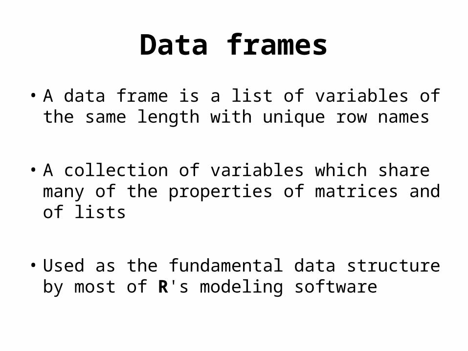
• A data frame is a list of variables of the same length with unique row names
• A collection of variables which share many of the properties of matrices and of lists
• Used as the fundamental data structure by most of R's modeling software
Data frames
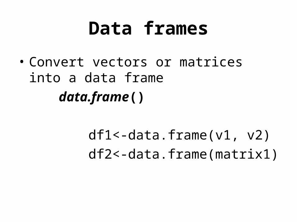
• Convert vectors or matrices into a data frame
data.frame()
df1<-data.frame(v1, v2)
df2<-data.frame(matrix1)
Data frames
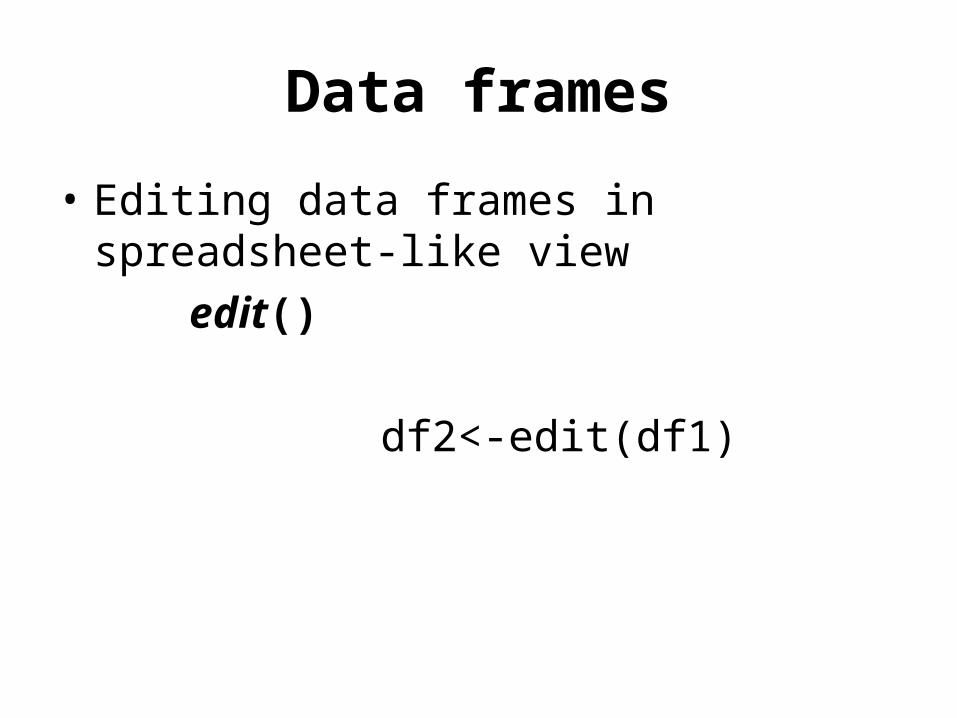
• Editing data frames in spreadsheet-like view
edit()
df2<-edit(df1)
• Let’s go to R and enter some vectors, arrays, and data frames
Script : QFC R short course R object types_1_vectors and arrays.R
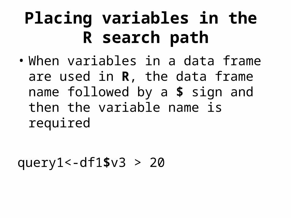
Placing variables in the R search path
• When variables in a data frame are used in R, the data frame name followed by a $ sign and then the variable name is required
query1<-df1$v3 > 20
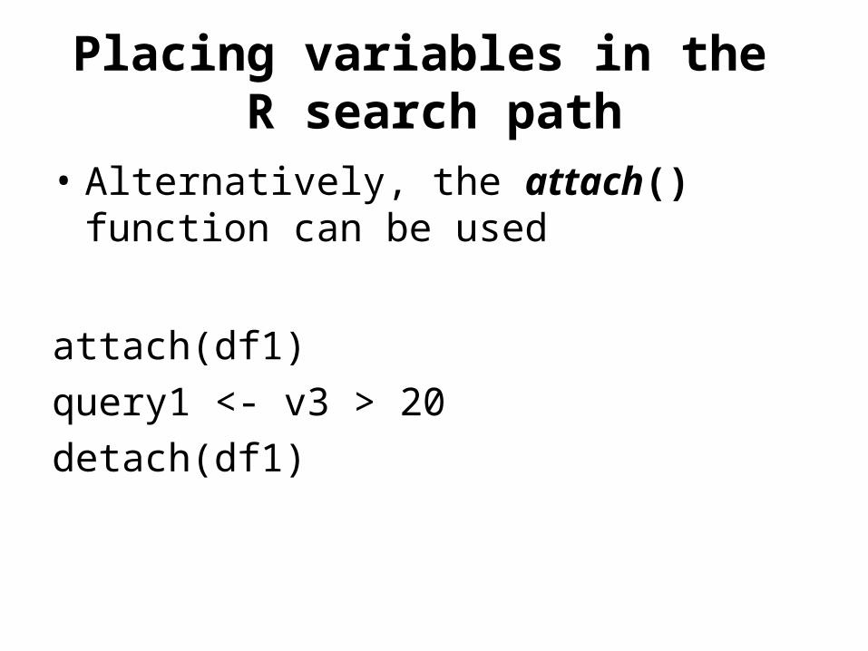
Placing variables in the R search path
• Alternatively, the attach() function can be used
attach(df1)
query1 <- v3 > 20
detach(df1)
Accessing data from an array, vector, or data frame
• Subscripts are used to extract data from objects in R
• Subscripts appear in square brackets and reference rows and columns, respectively
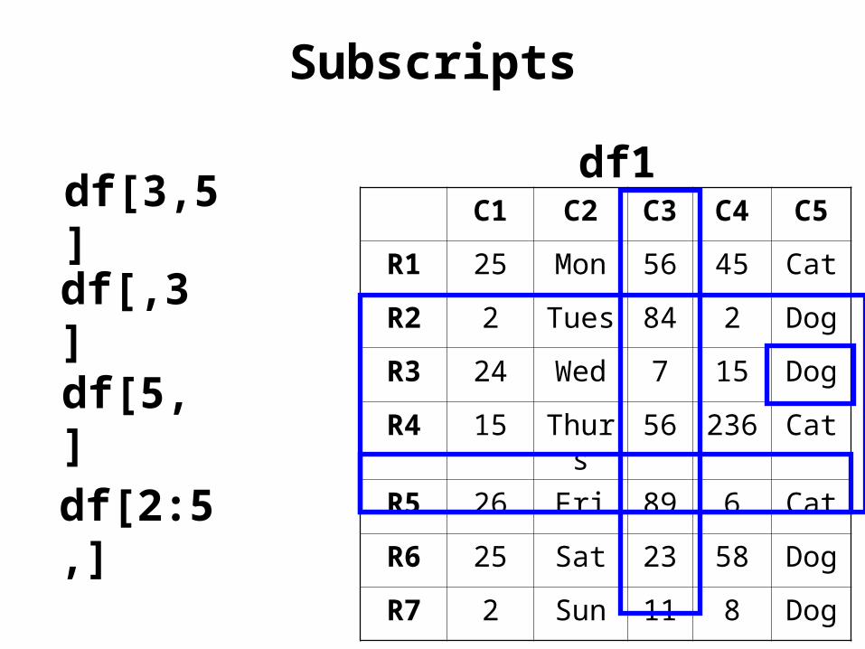
Subscripts
C1 C2 C3 C4 C5
R1 25 Mon 56 45 Cat
R2 2 Tues 84 2 Dog
R3 24 Wed 7 15 Dog
R4 15 Thurs 56 236 Cat
R5 26 Fri 89 6 Cat
R6 25 Sat 23 58 Dog
R7 2 Sun 11 8 Dog
df1df[3,5]
df[,3]
df[5,]
df[2:5,]
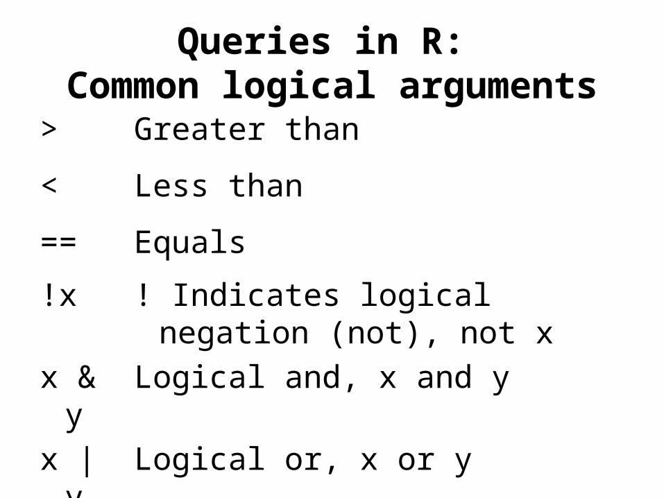
Queries in R: Common logical arguments
> Greater than
< Less than
== Equals
!x ! Indicates logical negation (not), not x
x & y Logical and, x and y
x | y Logical or, x or y
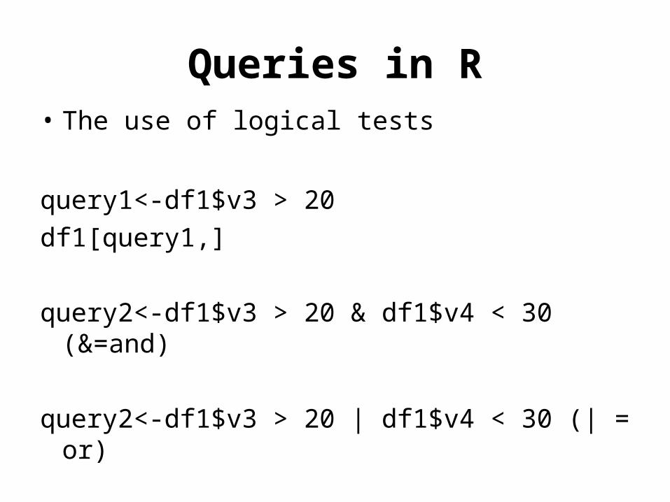
Queries in R• The use of logical tests
query1<-df1$v3 > 20
df1[query1,]
query2<-df1$v3 > 20 & df1$v4 < 30 (&=and)
query2<-df1$v3 > 20 | df1$v4 < 30 (| = or)

Queries in R
Script : QFC R short course R object types_2_query arrays data frames.R

Exercise 1
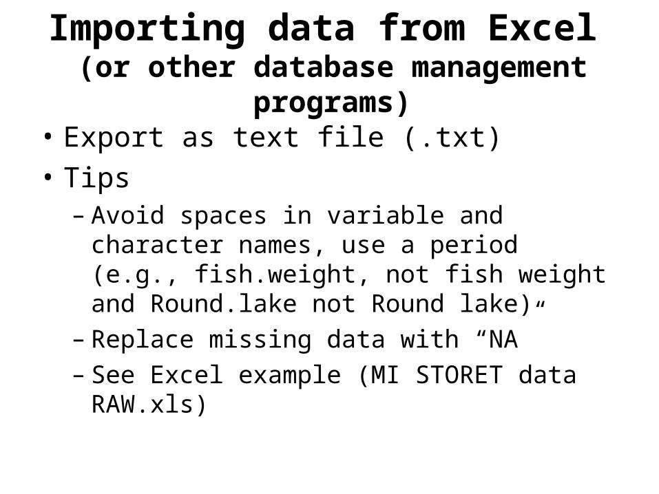
Importing data from Excel (or other database management programs)
• Export as text file (.txt)
• Tips– Avoid spaces in variable and character
names, use a period (e.g., fish.weight, not fish weight and Round.lake not Round lake)
– Replace missing data with “NA”– See Excel example (MI STORET data
RAW.xls)
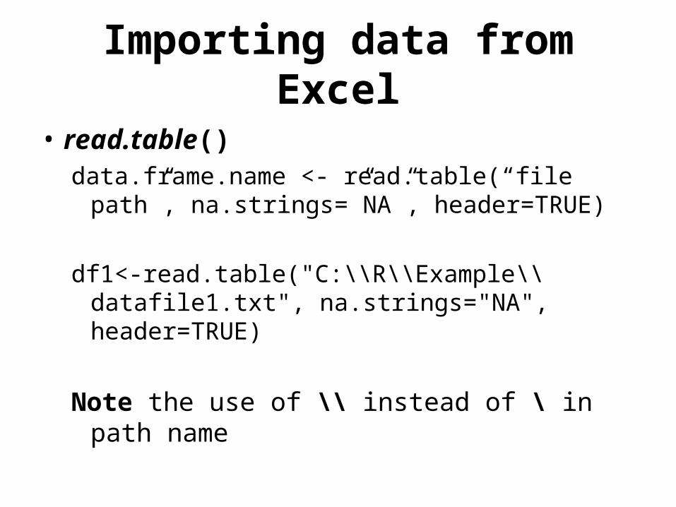
Importing data from Excel
• read.table()data.frame.name <- read.table(“file path”,
na.strings=”NA”, header=TRUE)
df1<-read.table("C:\\R\\Example\\datafile1.txt", na.strings="NA", header=TRUE)
Note the use of \\ instead of \ in path name

Importing data from Excel
• If your working directory is set, R will automatically look for the data text file there.
• So, the read.table syntax can be simplified by excluding the file path name:
• read.table(“data.txt”, na.strings=“NA”, header=T)
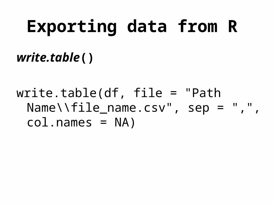
Exporting data from R
write.table()
write.table(df, file = "Path Name\\file_name.csv", sep = ",", col.names = NA)
Introduction to R functions
• R has many built-in functions and many more that can be downloaded from CRAN sites (Comprehensive R Archive Network)
• User-defined functions can also be created

The R base package
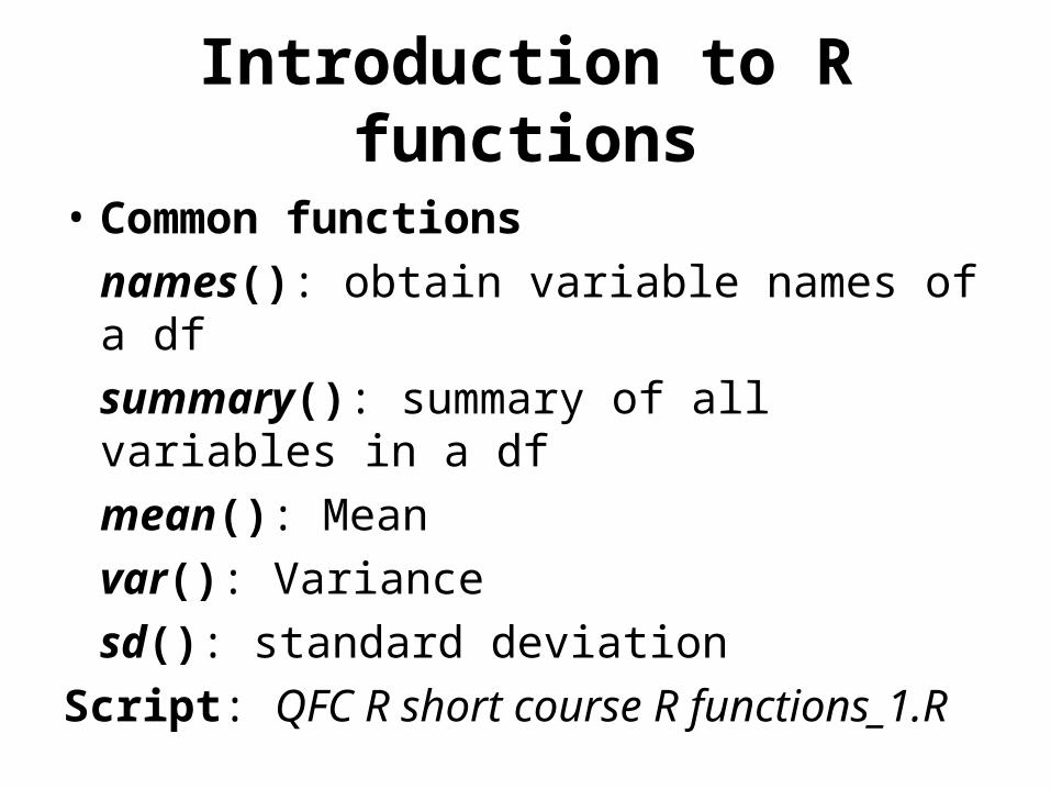
Introduction to R functions
• Common functions
names(): obtain variable names of a df
summary(): summary of all variables in a df
mean(): Mean
var(): Variance
sd(): standard deviation
Script: QFC R short course R functions_1.R
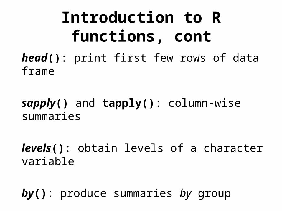
Introduction to R functions, cont
head(): print first few rows of data frame
sapply() and tapply(): column-wise summaries
levels(): obtain levels of a character variable
by(): produce summaries by group
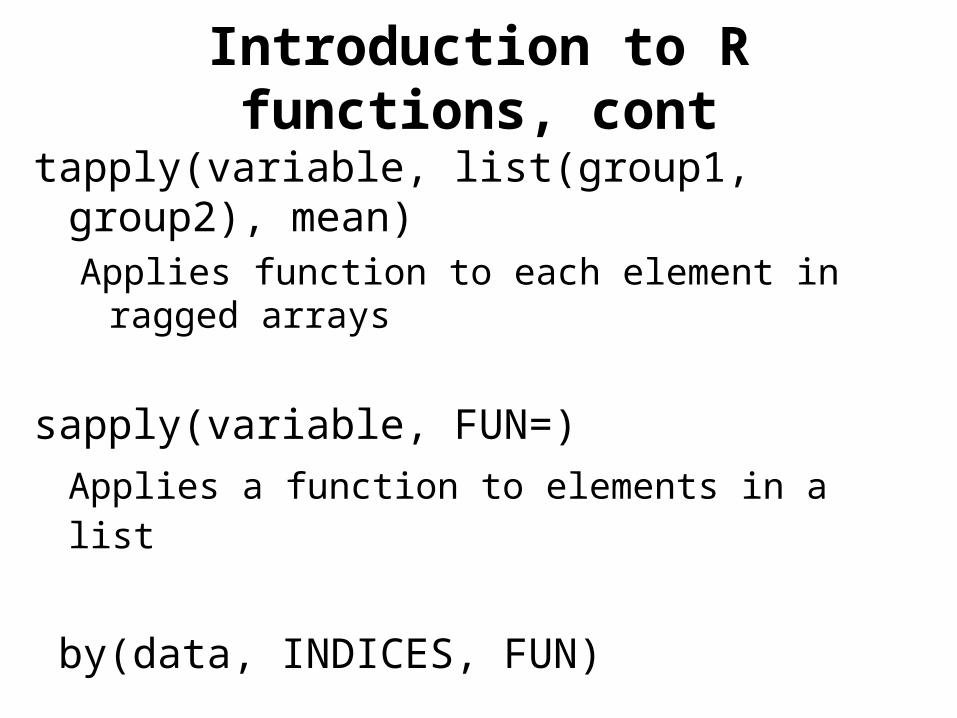
Introduction to R functions, cont
tapply(variable, list(group1, group2), mean)Applies function to each element in ragged arrays
sapply(variable, FUN=)
Applies a function to elements in a list
by(data, INDICES, FUN)
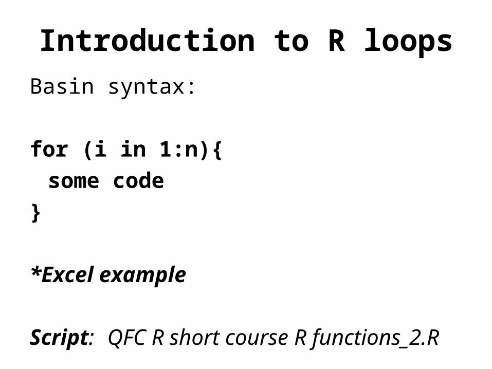
Introduction to R loops
Basin syntax:
for (i in 1:n){
some code
}
*Excel example
Script: QFC R short course R functions_2.R
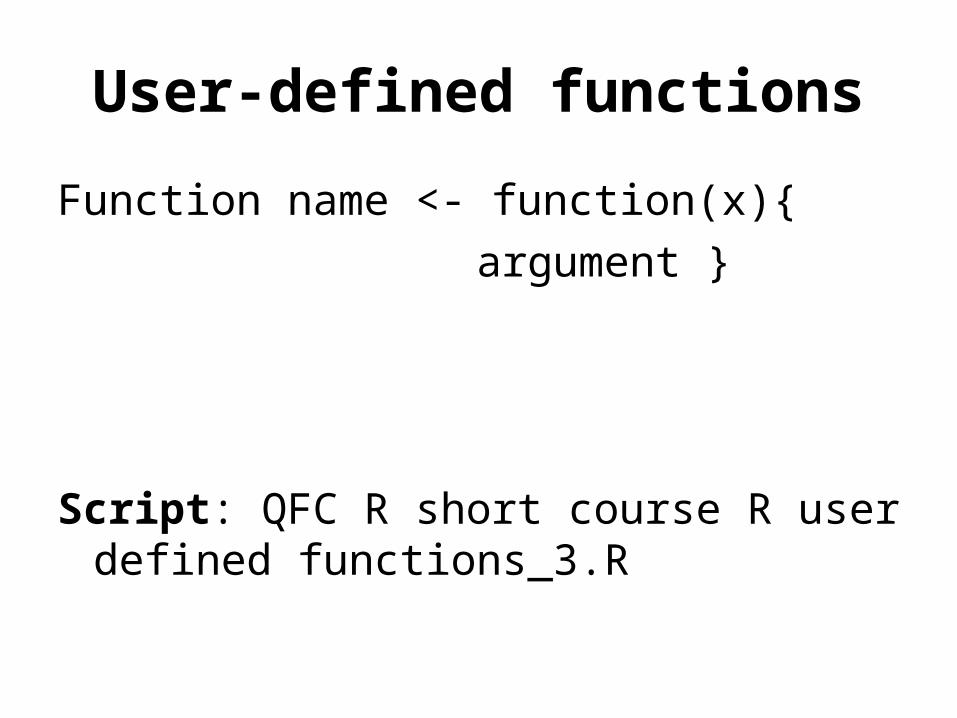
User-defined functions
Function name <- function(x){
argument }
Script: QFC R short course R user defined functions_3.R

Exercise 2 (Part 1)
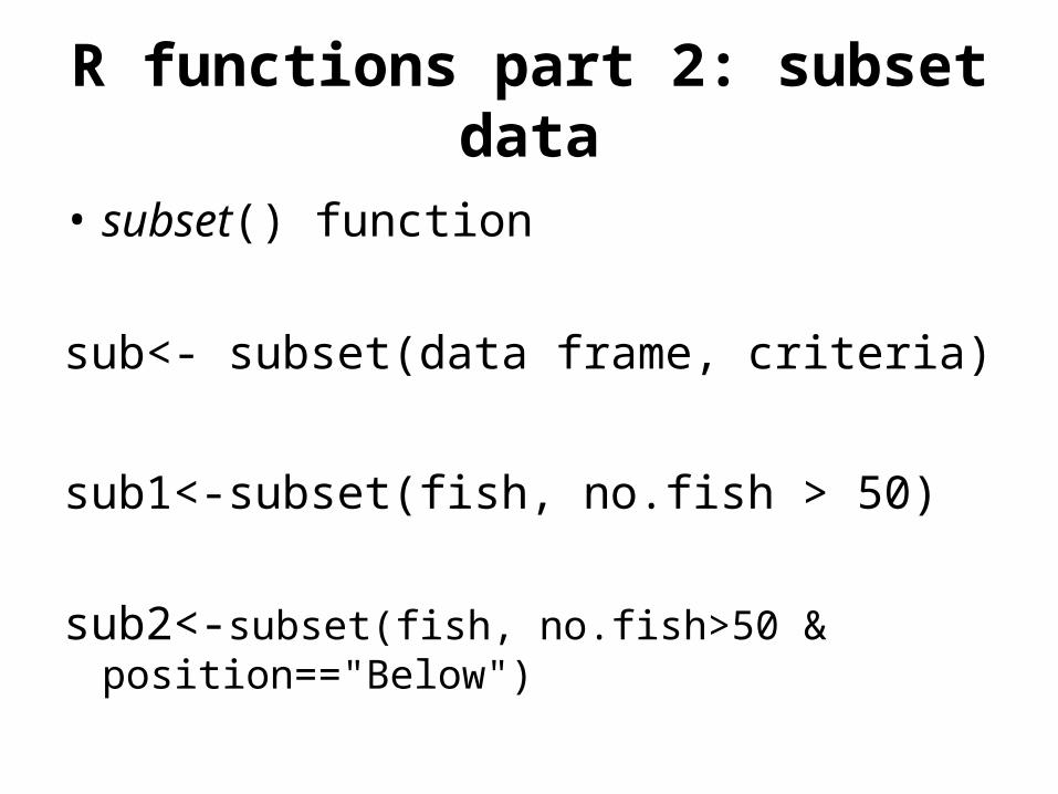
R functions part 2: subset data
• subset() function
sub<- subset(data frame, criteria)
sub1<-subset(fish, no.fish > 50)
sub2<-subset(fish, no.fish>50 & position=="Below")
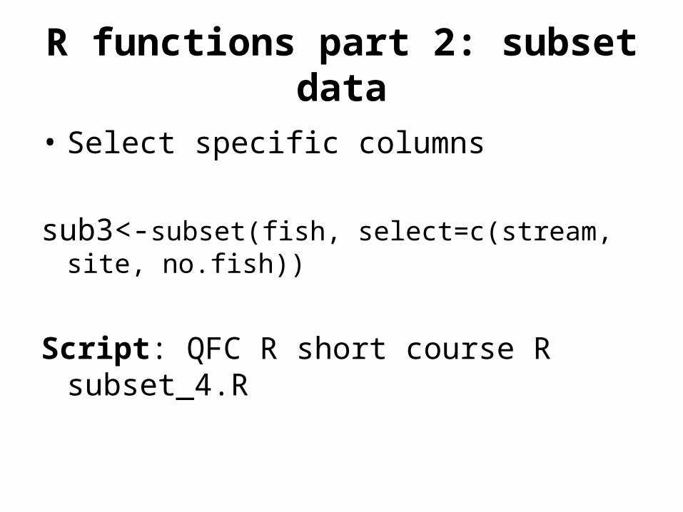
R functions part 2: subset data
• Select specific columns
sub3<-subset(fish, select=c(stream, site, no.fish))
Script: QFC R short course R subset_4.R
Exercise 2 (Part 2)
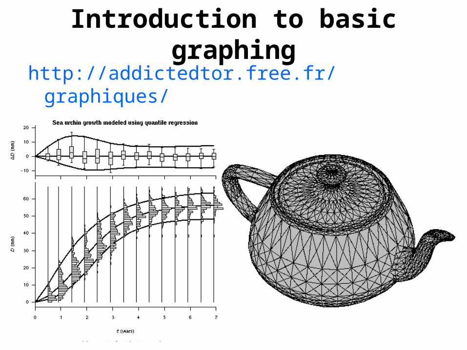
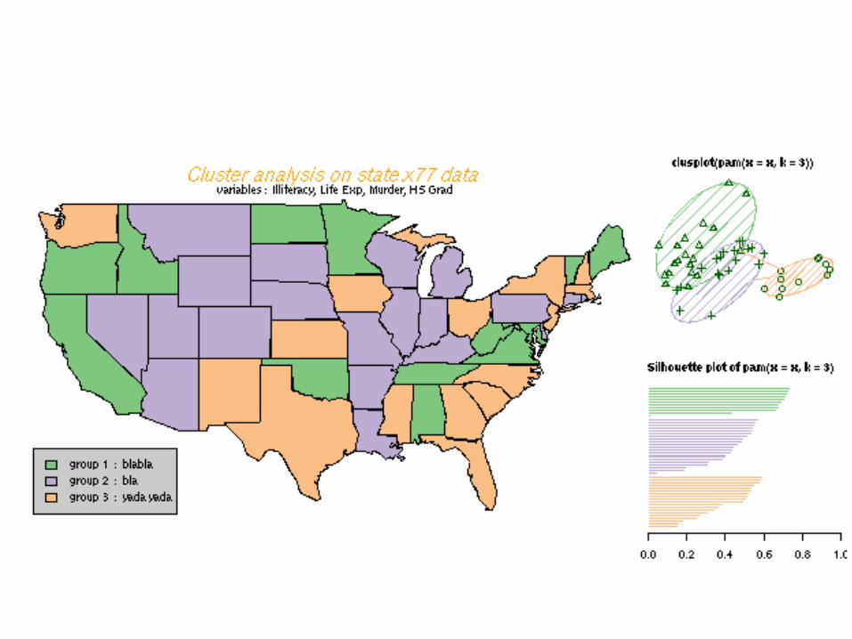
Introduction to basic graphing
http://addictedtor.free.fr/graphiques/
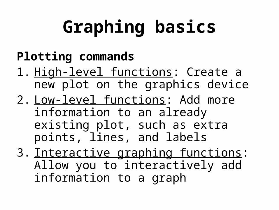
Graphing basics
Plotting commands1. High-level functions: Create a new plot
on the graphics device2. Low-level functions: Add more
information to an already existing plot, such as extra points, lines, and labels
3. Interactive graphing functions: Allow you to interactively add information to a graph

Common high-level functions
• plot(): A generic function that produces a type of plot that is dependent on the type of the first arguement
• hist(): Creates a histogram of frequencies
• barplot(): Creates a histogram of values
• boxplot(): Creates a boxplot
• pairs(): Creates a scatter plot matrix
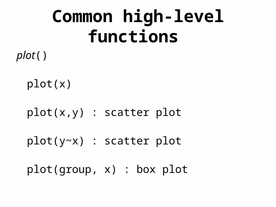
Common high-level functions
plot()
plot(x)
plot(x,y) : scatter plot
plot(y~x) : scatter plot
plot(group, x) : box plot
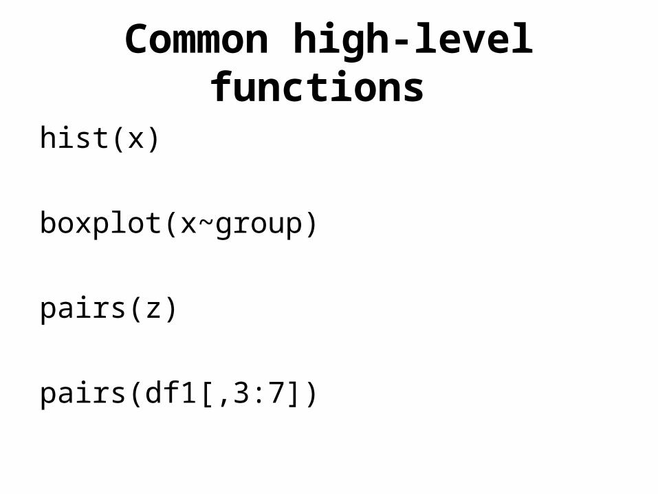
Common high-level functions
hist(x)
boxplot(x~group)
pairs(z)
pairs(df1[,3:7])
Common high-level functions
Script:
QFC R course Graphing Basics_1.R

Exercise 3

END OF DAY 1
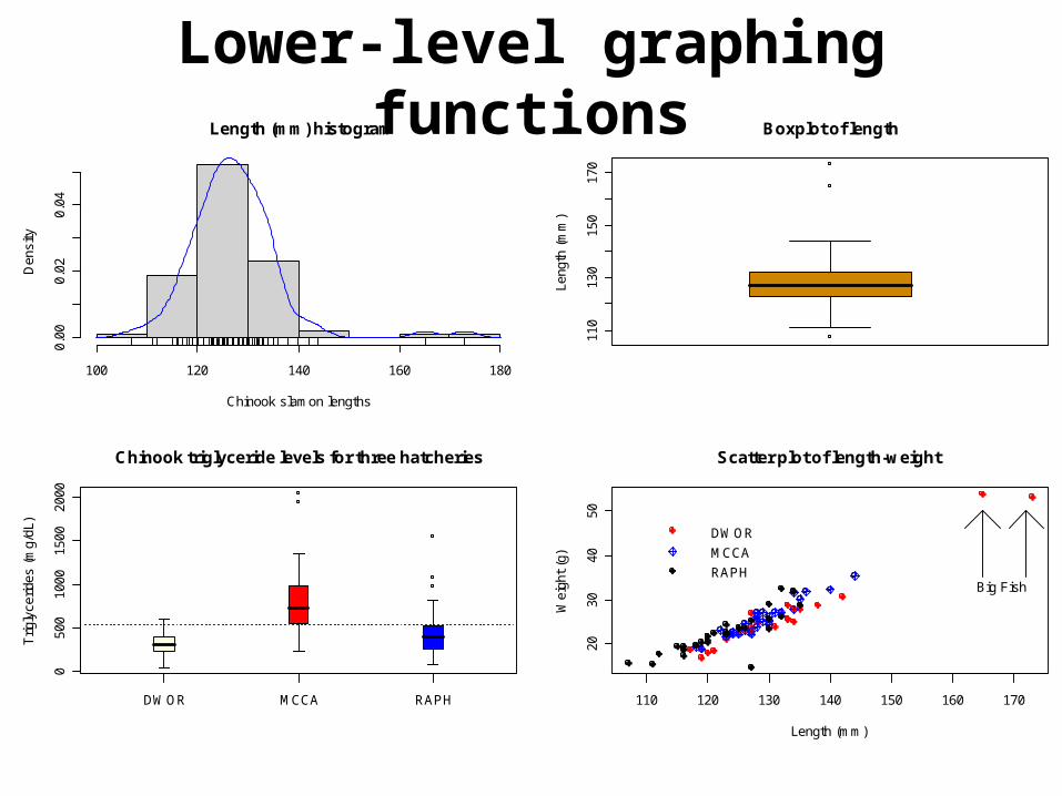
Lower-level graphing functionsLength (mm) histogram
Chinook slamon lengths
Den
sity
100 120 140 160 180
0.00
0.02
0.04
110
130
150
170
Boxplot of length
Leng
th (
mm
)
DWOR MCCA RAPH
050
010
0015
0020
00
Chinook triglyceride levels for three hatcheries
Trig
lyce
rides
(m
g/dL
)
110 120 130 140 150 160 170
2030
4050
Scatter plot of length-weight
Length (mm)
Wei
ght
(g)
DWOR
MCCA
RAPHBig Fish
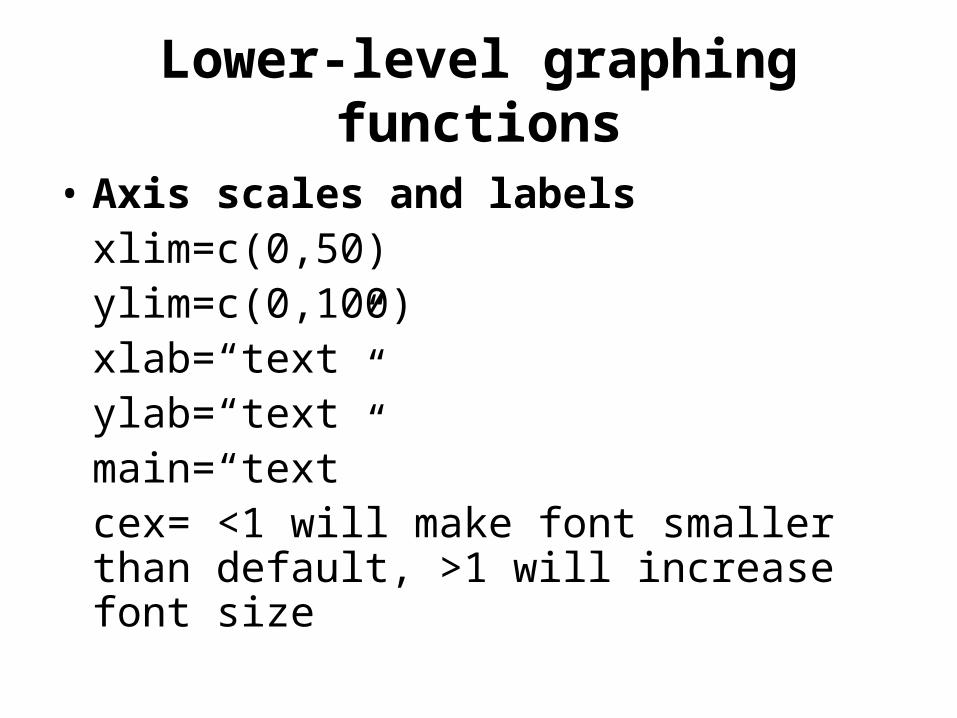
Lower-level graphing functions
• Axis scales and labelsxlim=c(0,50)ylim=c(0,100)xlab=“text”ylab=“text”main=“text”cex= <1 will make font smaller than default, >1 will increase font size
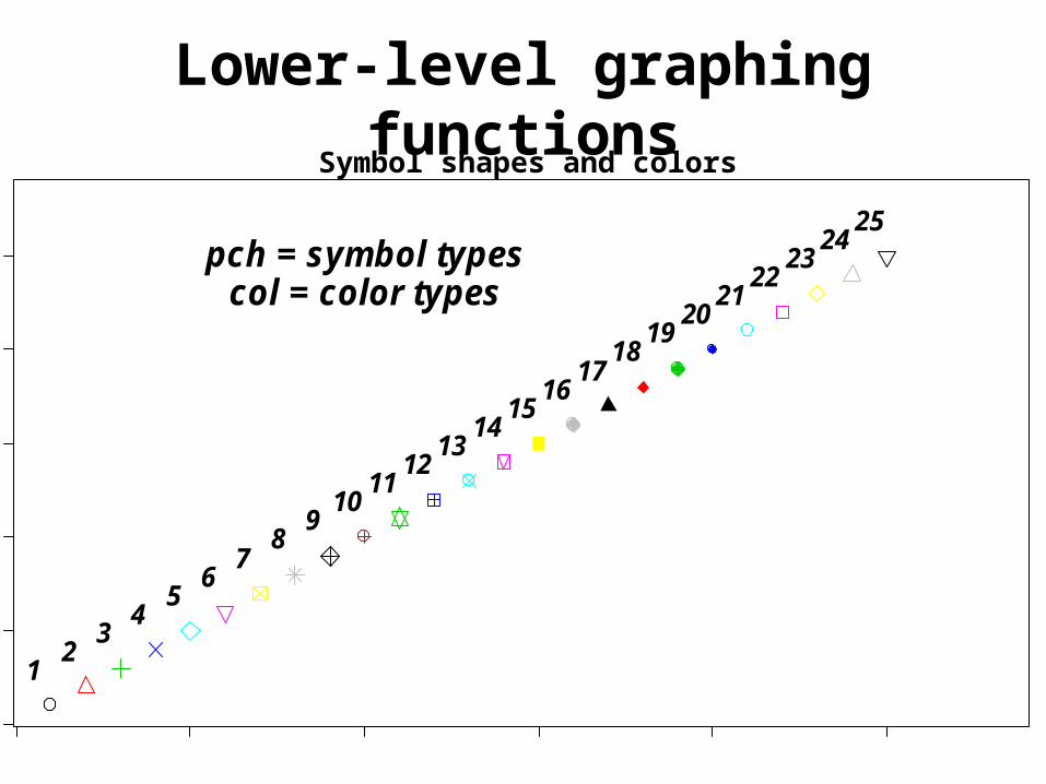
Lower-level graphing functions
0 5 10 15 20 25
05
1015
2025 pch = symbol types
col = color types
12
34
56
78
910
1112
1314
1516
1718
1920
2122
2324
25
Symbol shapes and colors
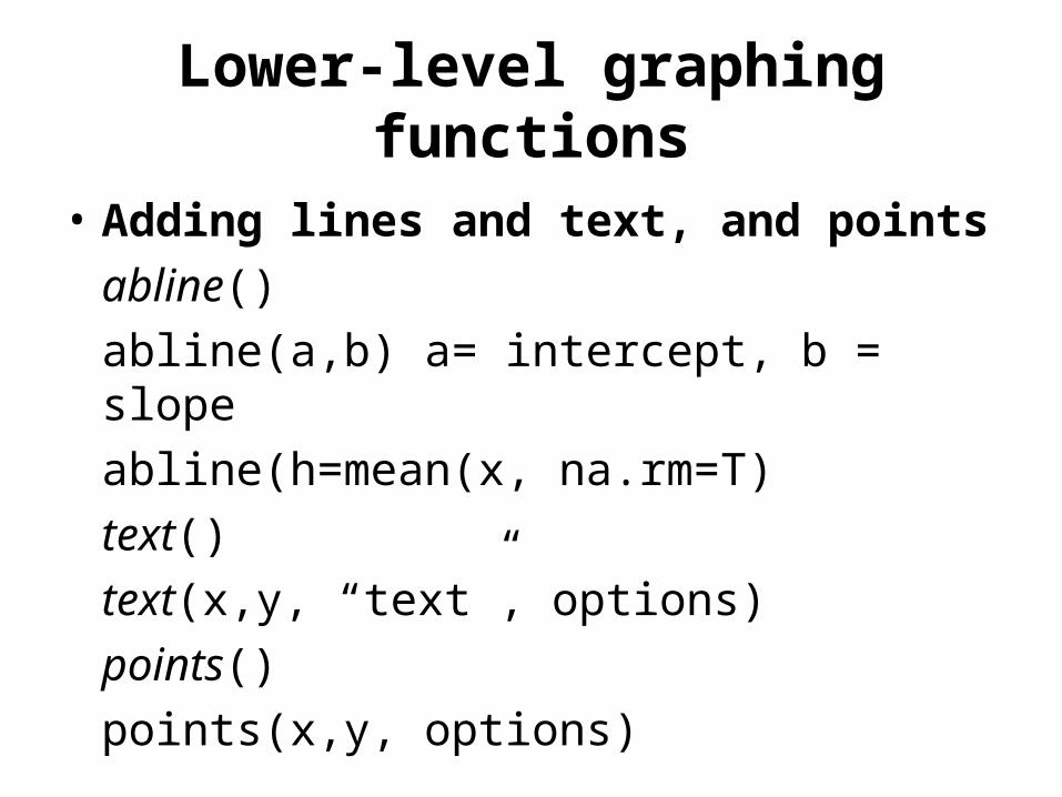
Lower-level graphing functions
• Adding lines and text, and points
abline()
abline(a,b) a= intercept, b = slope
abline(h=mean(x, na.rm=T)
text()
text(x,y, “text”, options)
points()
points(x,y, options)
Lower-level graphing functions
Scripts:
QFC R course Graphing Basics_2.R
QFC R course Graphing Basics_3.R

Exercise 4
Introduction to statistical analyses
• R provides many functions for statistical analyses– Descriptive– Univariate– Multivariate– Mixed models– Spatial– Bayesian
Introduction to statistical analyses
•Descriptive statistics
Correlations: cor()
cor(df1[,2:6])
t-tests: t.test()
t.test(y~group)
Script:
QFC R short course correlations and t-test.R
Basic model structure in R
response variable ~ predictor variable(s)
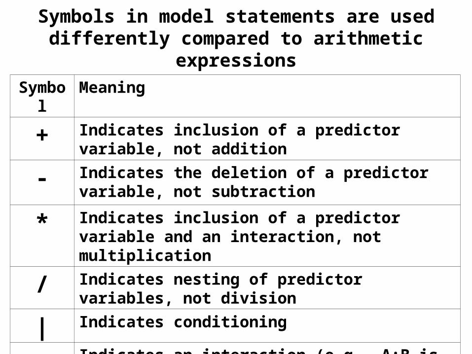
Symbols in model statements are used differently compared to arithmetic expressions
Symbol Meaning
+ Indicates inclusion of a predictor variable, not addition
- Indicates the deletion of a predictor variable, not subtraction
* Indicates inclusion of a predictor variable and an interaction, not multiplication
/ Indicates nesting of predictor variables, not division
| Indicates conditioning
: Indicates an interaction (e.g., A:B is a two-way interaction between A and B)
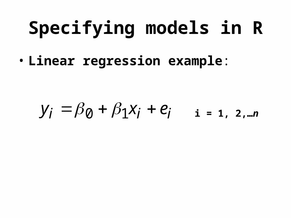
Specifying models in R
• Linear regression example:
iii exy 10 i = 1, 2,…n
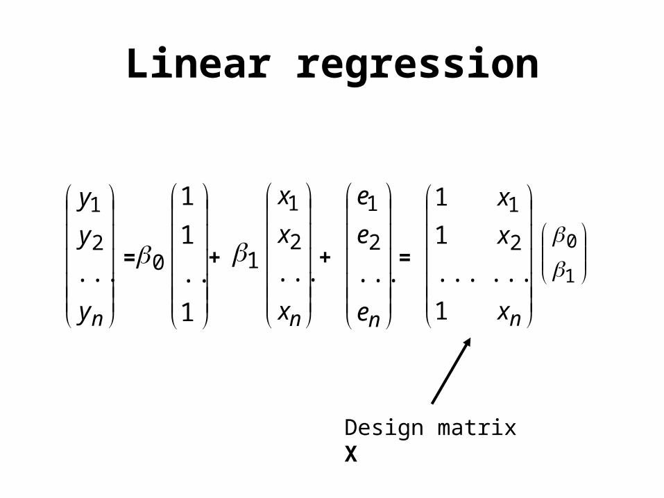
Linear regression
ny
y
y
...2
1
= 0
1
...
1
1
+ 1
nx
x
x
...2
1
+
ne
e
e
...2
1
=
nx
x
x
1
......
1
1
2
1
1
0
Design matrix X
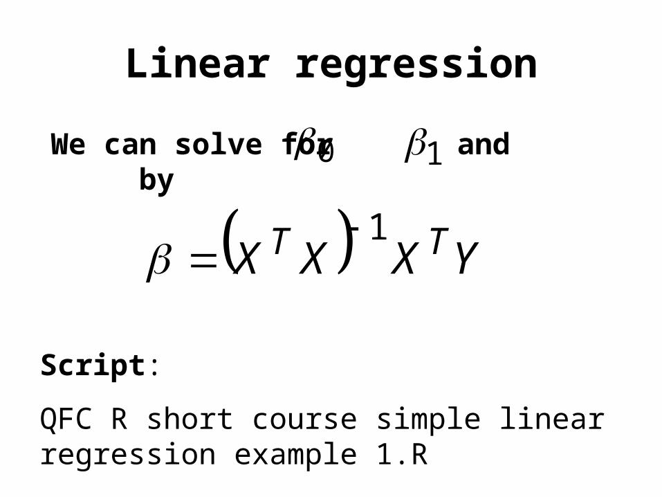
Linear regression
YXXX TT 1
We can solve for and by0 1
Script:
QFC R short course simple linear regression example 1.R
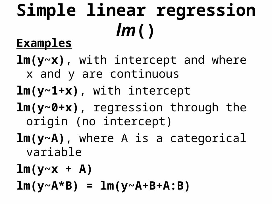
Simple linear regression lm()Examples
lm(y~x), with intercept and where x and y are continuous
lm(y~1+x), with intercept
lm(y~0+x), regression through the origin (no intercept)
lm(y~A), where A is a categorical variable
lm(y~x + A)
lm(y~A*B) = lm(y~A+B+A:B)
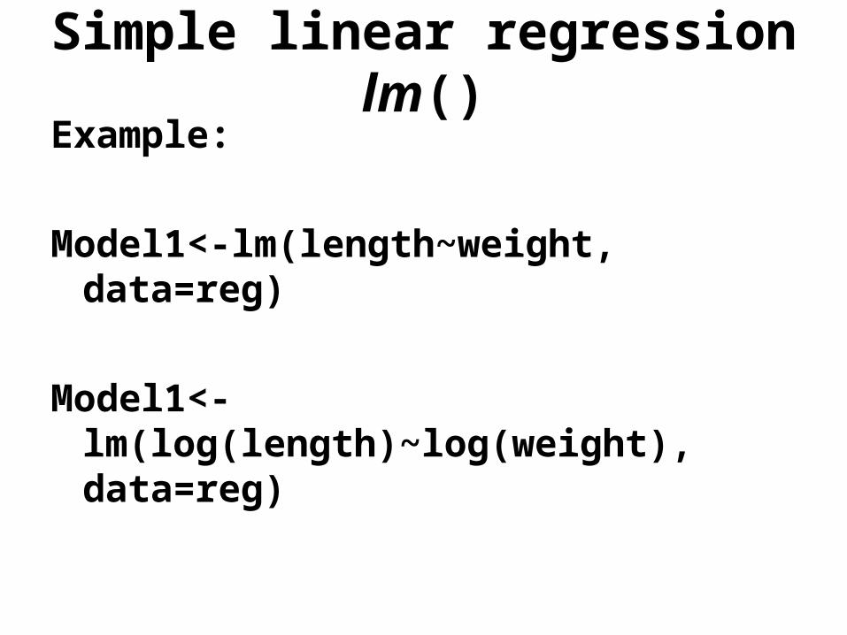
Simple linear regression lm()Example:
Model1<-lm(length~weight, data=reg)
Model1<-lm(log(length)~log(weight), data=reg)
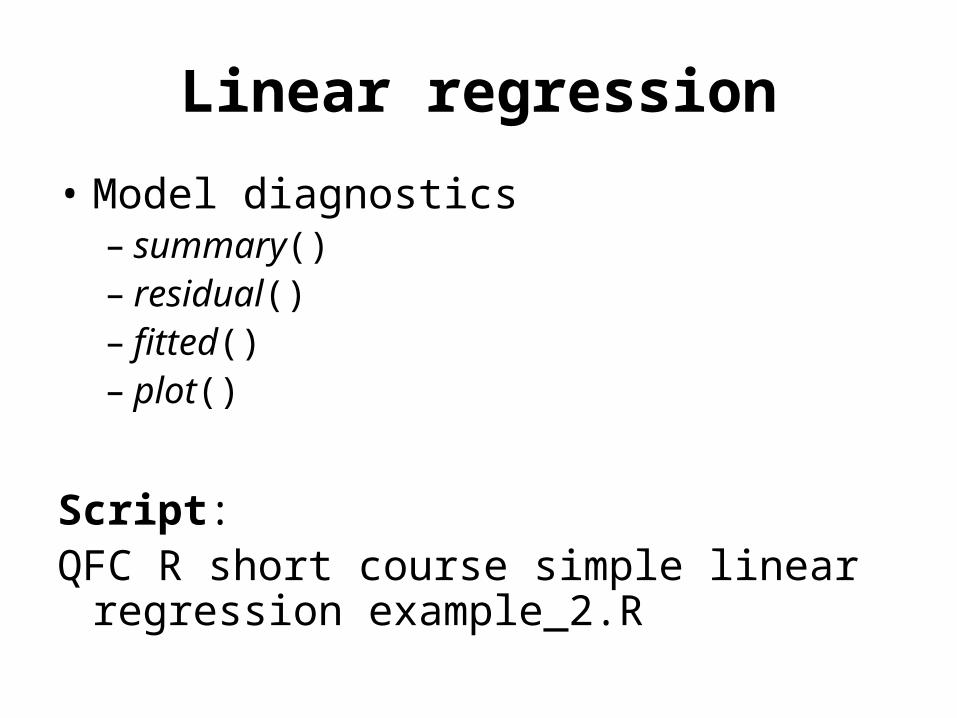
Linear regression
• Model diagnostics– summary()– residual()– fitted()– plot()
Script:QFC R short course simple linear regression
example_2.R
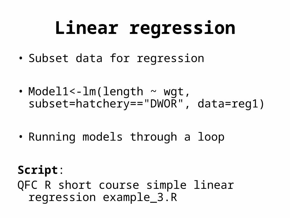
Linear regression
• Subset data for regression
• Model1<-lm(length ~ wgt, subset=hatchery=="DWOR", data=reg1)
• Running models through a loop
Script:QFC R short course simple linear regression
example_3.R
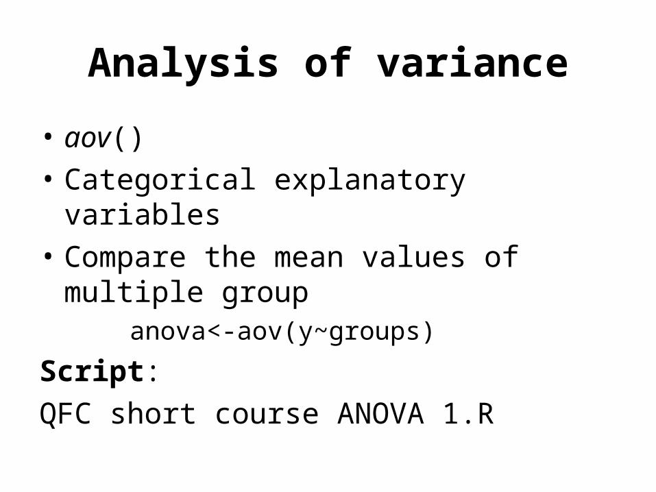
Analysis of variance
• aov()
• Categorical explanatory variables
• Compare the mean values of multiple group
anova<-aov(y~groups)
Script:
QFC short course ANOVA 1.R
Exercise 5
Nonlinear regression
• Estimating parameters is more tricky compared to linear regression models
• Iterative search procedure required
• Must provide starting values of parameters
• Convergence issues
Nonlinear regression
Differences in R between linear and nonlinear regression
1.For nonlinear regression models the user must specify the exact equation as part of the model statement
2.The user must specify initial guesses as to the value of the parameters that are being estimated
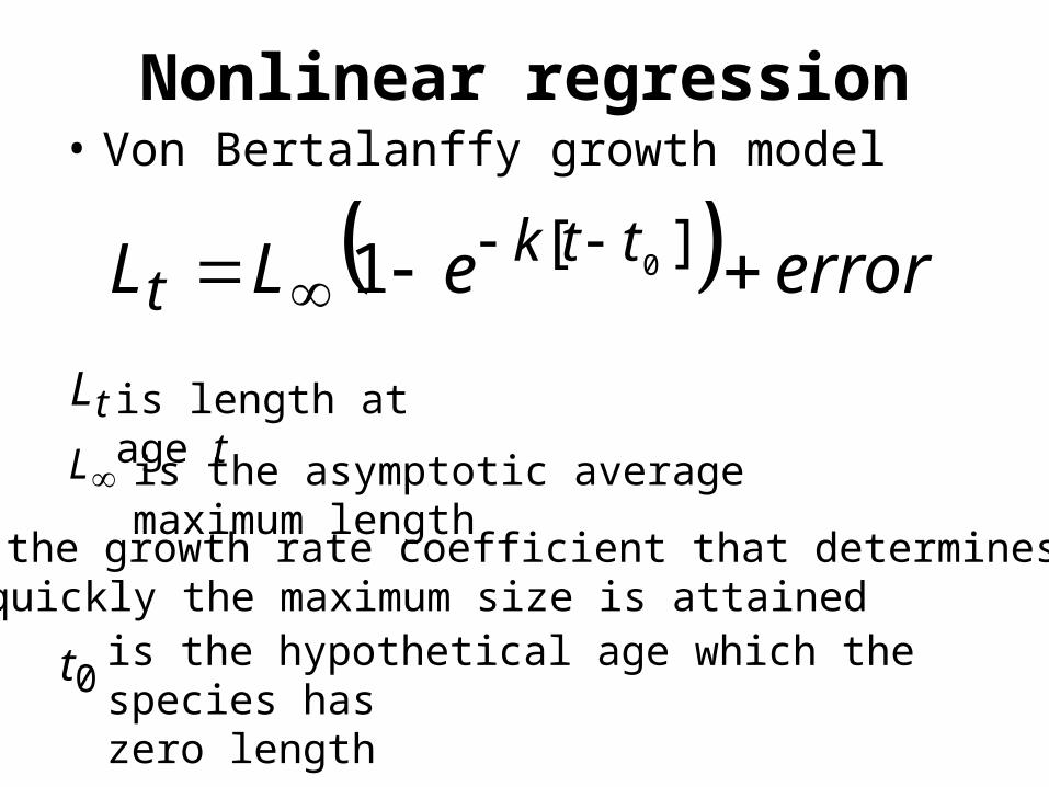
Nonlinear regression• Von Bertalanffy growth model
erroreLL ttkt
][ 01
tL is length at age t
L is the asymptotic average maximum length
k is the growth rate coefficient that determines how quickly the maximum size is attained
0t is the hypothetical age which the species has zero length
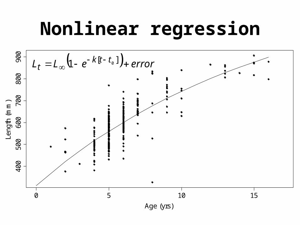
Nonlinear regression
0 5 10 15
400
500
600
700
800
900
Age (yrs)
Leng
th (
mm
)
erroreLL ttkt
][ 01
Nonlinear regression
nls()
Least-squares estimates of the parameters of a nonlinear model
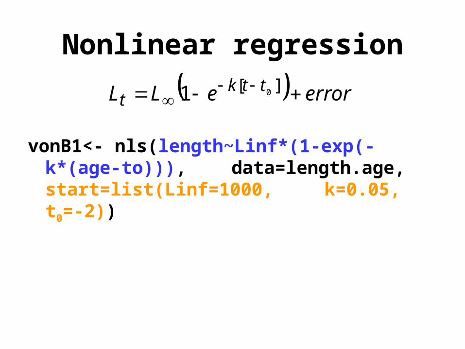
Nonlinear regression
vonB1<- nls(length~Linf*(1-exp(-k*(age-to))), data=length.age, start=list(Linf=1000, k=0.05, t0=-2))
erroreLL ttkt
][ 01

Nonlinear regressionGraphing fitted lines:1. Generate a sequence of numbers that cover
the range of the x-axis
2. Generate predicted values for the sequence of x-values
3. Plot original data
4. Overlay predicted values
Nonlinear regression
Script:
QFC R course Von Bertalanffy Nonlinear regression.R
Exercise 6