An introduction to the theory of interferometry EuroSummer School Observation and data reduction...
64
An introduction to the theory of interferometry EuroSummer School Observation and data reduction with the Very Large Telescope Interferometer Goutelas, France June 4-16, 2006 C.A.Haniff Astrophysics Group, Department of Physics, University of Cambridge, UK 5 th June 2006
-
Upload
briana-wilson -
Category
Documents
-
view
216 -
download
0
Transcript of An introduction to the theory of interferometry EuroSummer School Observation and data reduction...
An introduction to the theory of interferometry
EuroSummer School
Observation and data reduction with the Very Large Telescope Interferometer
Goutelas, FranceJune 4-16, 2006
C.A.Haniff
Astrophysics Group, Department of Physics,University of Cambridge, UK
5th June 2006
VLTI EuroSummer School 25th June 2006C.A.Haniff – The theory of interferometry
PreamblePreamble
• Learning interferometry is like learning any new skill (e.g. walking):– You have to want to learn.– You start by crawling, then you walk, then you run.– Having fancy shoes doesn’t help at the start.– You don’t have to know how shoes are made.– At some stage you will need to learn where to walk to.
• This is a school:– You should assume nothing, as I will!– We have a lot to cover – this will not be easy.– Knowing what questions to ask is what is important.– Please ask, again and again if necessary.
• I’m not here to “sell” interferometry, I’m here to help you understand it.
VLTI EuroSummer School 35th June 2006C.A.Haniff – The theory of interferometry
OutlineOutline
• Image formation with conventional telescopes– The diffraction limit– Incoherent imaging equation– Fourier decomposition
• Coherence functions– Temporal coherence– Spatial coherence
• Interferometric measurements– Fringe parameters– The van-Cittert Zernike theorem
• Imaging with interferometers– Rules of thumb– Interferometric images– Sensitivity

VLTI EuroSummer School 45th June 2006C.A.Haniff – The theory of interferometry
OutlineOutline
• Image formation with conventional telescopes– The diffraction limit– Incoherent imaging equation– Fourier decomposition
• Coherence functions– Temporal coherence– Spatial coherence
• Interferometric measurements– Fringe parameters– The van-Cittert Zernike theorem
• Imaging with interferometers– Rules of thumb– Interferometric images– Sensitivity

VLTI EuroSummer School 55th June 2006C.A.Haniff – The theory of interferometry
Terminology and rationaleTerminology and rationale
• High spatial resolution: the ability to recover information on small angular scales:– Positions.– Basic information - scale sizes, morphology, etc.– Detailed image structure.
• Bandpasses:– Optical 0.3-1.0 m.– Near-infrared 1.0-2.2 m.– Thermal-infrared 3.5-20.0 m.
• What limits our ability to investigate sources at high spatial resolution?– The wave nature of light.– The Earth’s atmosphere.

VLTI EuroSummer School 65th June 2006C.A.Haniff – The theory of interferometry
What do we observe?What do we observe?
• Consider a perfect telescope in space observing an unresolved point source:
– This produces an Airy pattern witha characteristic width: 1.22Din its focal plane.
is the approximate angular widthof the image, called the “angularresolution”.
is the wavelength at which theobservation is made.
– D is the diameter of the telescopeaperture, assumed circular here.

VLTI EuroSummer School 75th June 2006C.A.Haniff – The theory of interferometry
How does this impact imaging?How does this impact imaging?
• Image formation (under incoherent & isoplanatic conditions):
– Each point in the source produces a displaced Airy pattern. The superposition of these limits the detail visible in the final image.
• But what causes the Airy pattern?
– Interference between parts of the wavefront that originate from different regions of the aperture.
– In this case, the relative amplitude and phase of the field at each part of the aperture are what matter.
VLTI EuroSummer School 85th June 2006C.A.Haniff – The theory of interferometry
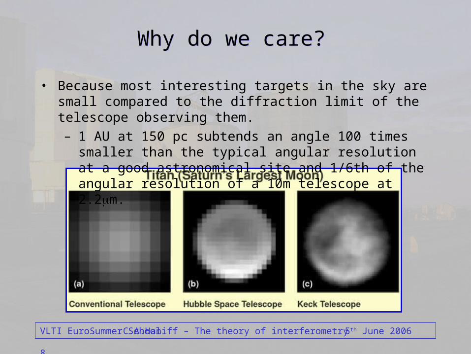
Why do we care? Why do we care?
• Because most interesting targets in the sky are small compared to the diffraction limit of the telescope observing them.
– 1 AU at 150 pc subtends an angle 100 times smaller than the typical angular resolution at a good astronomical site and 1/6th of the angular resolution of a 10m telescope at 2.2m.
VLTI EuroSummer School 95th June 2006C.A.Haniff – The theory of interferometry
Image formation with conventional telescopesImage formation with conventional telescopes
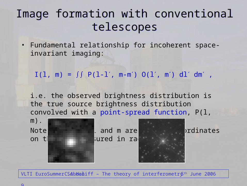
• Fundamental relationship for incoherent space-invariant imaging:
I(l, m) = P(l-l, m-m) O(l, m) dl dm ,
i.e. the observed brightness distribution is the true source brightness distribution convolved with a point-spread function, P(l, m).
Note that here l and m are angular coordinates on the sky, measured in radians.
VLTI EuroSummer School 105th June 2006C.A.Haniff – The theory of interferometry
An alternative representationAn alternative representation
• This convolutional relationship, which typifies the behaviour of linear space-invariant (isoplanatic) systems, can be written alternatively, by taking the Fourier transform of each side of the equation, to give:
I(u, v) = T(u, v) O(u, v) ,
where italic functions refer to the Fourier transforms of their roman counterparts, and u and v are now spatial frequencies measured in radians-1.
• Importantly, the essential properties of the imaging system are encapsulated in a complex multiplicative transfer function, T(u, v).
• Note that this is nothing more than the Fourier transform of the PSF.
VLTI EuroSummer School 115th June 2006C.A.Haniff – The theory of interferometry
The Transfer functionThe Transfer function
• In general the transfer function is obtained from the auto-correlation of the complex pupil function:
T(u, v) = P(x, y) P(x+u, y+v) dx dy ,
where x and y denote co-ordinates in the pupil.
• A number of key features of this formalism are worth noting:– For each spatial frequency, u, there is a physical baseline, B, in the
pupil, of length u.
– In the absence of aberrations P(x, y) is equal to 1 where the aperture is transmitting and 0 otherwise.
– For a circularly symmetric aperture, the transfer function can be written as a function of a single co-ordinate: T(f), with f2 = u2 + v2.

VLTI EuroSummer School 125th June 2006C.A.Haniff – The theory of interferometry
The example of a circular apertureThe example of a circular aperture
• T(f) falls smoothly tozero at fmax = D/.
• The PSF is the familiarAiry pattern.
• The full-width at half-maximum of this is atapproximately 0.9 /D.

VLTI EuroSummer School 135th June 2006C.A.Haniff – The theory of interferometry
What should we learn from all this?What should we learn from all this?
• Decomposition of an image into a series of spatially separated compact PSFs.
• The equivalence of this to a superposition of non-localized sinusoids.
• The description of an image in terms of its Fourier components.
• The action of an incoherent imaging system as a filter for the true spatial Fourier spectrum of the source.
• The association of each Fourier component (or spatial frequency) with a distinct physical baseline in the aperture that samples the light.
• The form of the point-spread function as arising from the relative sampling (and hence weighting given to) the different spatial frequencies (and hence baselines) measured by the pupil of the imaging system.

VLTI EuroSummer School 145th June 2006C.A.Haniff – The theory of interferometry
OutlineOutline
• Image formation with conventional telescopes– The diffraction limit– Incoherent imaging equation– Fourier decomposition
• Coherence functions– Temporal coherence– Spatial coherence
• Interferometric measurements– Fringe parameters– The van-Cittert Zernike theorem
• Imaging with interferometers– Rules of thumb– Interferometric images– Sensitivity

VLTI EuroSummer School 155th June 2006C.A.Haniff – The theory of interferometry
Coherence functionsCoherence functions
• In the context of interferometric imaging it is sometimes useful to consider the spatio-temporal correlations of the field arising from an astronomical source:
• This means interrogating the electric field producedby the source at some locations and looking atthe correlations between these measured fields.
• The reason for doing this is that the spectral andspatial properties of the source can, in principle,be recovered from these measurements withoutusing any other apparatus.
This is imaging without a telescope!

VLTI EuroSummer School 165th June 2006C.A.Haniff – The theory of interferometry
The temporal and spatial coherence functionsThe temporal and spatial coherence functions
• Measure electric field from a distant sourceat two locations r1 and r2 at times t1 and t2.
• Each field is composed of contributionsfrom each element of the source.
• We define the spatio-temporal coherence functionas V(r1, t1, r2, t2) = E(r1, t1) E(r2, t2).
• We are interested in two special cases:
– t1 = t2 : spatial coherence function.
– r1 = r2 : temporal coherence function.

VLTI EuroSummer School 175th June 2006C.A.Haniff – The theory of interferometry
– The coherence function does not depend on r1.
– It is a function of a time delay, = t1t2.
– It quantifies the extent to which the fields alonga given wave train are correlated.
– It is related to the quantity that alaboratory Michelson interferometermeasures.
The temporal coherence functionThe temporal coherence function
• For astronomical sources, this coherence function can be written as:
E(r1, t1) E(r1, t2) = V(t1t2) = V() .
• In this case we should note that:

VLTI EuroSummer School 185th June 2006C.A.Haniff – The theory of interferometry
Use of the temporal coherence functionUse of the temporal coherence function
• The importance of the temporal coherence function arises from an important result in physics, the Wiener-Khintchine theorem.
• This says that the normalized value of the temporal coherence function V() is equal to the normalized Fourier transform of the spectral energy distribution, B(), of the source:
V() = B() ei d B()d .– A broad spectral energy distribution leads to a coherence function
that decays rapidly since and are reciprocal coordinates.
– We can define a coherence time: coh 1/, with = /2 the spectral bandwidth of the radiation.
Measurements of V() allow recovery of the source spectrum.

VLTI EuroSummer School 195th June 2006C.A.Haniff – The theory of interferometry
The spatial coherence functionThe spatial coherence function
• For astronomical sources, this coherence function can be written as:
E(r1, t1) E(r2, t1) = V(r1r2) = V() .
• In this case we see that:– This coherence function does not depend on t1.
– It is a function of a vector separation, = r1r2.
– It quantifies the correlations between differentspatial locations on a wavefront.
– It corresponds to the quantity that a Young’sslit experiment investigates (on axis).

VLTI EuroSummer School 205th June 2006C.A.Haniff – The theory of interferometry
Use of the spatial coherence functionUse of the spatial coherence function
• The importance of the spatial coherence function arises from another important result in physics, the van Cittert-Zernike theorem.
• This states that, for incoherent sources in the far-field, the normalized value of the spatial coherence function V() is equal to the normalized Fourier transform of the brightness distribution in the sky, I():
V() = I() ei 2/ () d I() d ,
or in slightly different notation:
V(u, v) = I(l, m) ei2(ul + vm) dl dm I(l, m) dl dm ,
where u and v are the components of the baseline measured in wavelengths, and l and m are angular coordinates on the sky.

VLTI EuroSummer School 215th June 2006C.A.Haniff – The theory of interferometry
What should we draw from all this? What should we draw from all this?
• Measurements of these coherence functions allow us to interrogate a source without using a conventional imaging telescope or spectrometer.
• This in turn relies upon access to measurements of time-averaged products of field quantities like E(r1) E(r2) .
• The relationships between the source parameters and the coherence functions are Fourier transforms. Hence these are:– Linear.
– Invertible.
– Complex.
• We note the mathematical equivalence of the spatial coherence function V(=0, ) and the Fourier decomposition of an image we referred to earlier.
VLTI EuroSummer School 225th June 2006C.A.Haniff – The theory of interferometry
Linking these first two sections of our lectureLinking these first two sections of our lecture
• Here is how we can put this all together:
– We can describe a source in the sky as a superposition of co-sinusoids, each of which corresponds to a given spatial frequency.
– Measurements of the coherence function are in fact measurements of the strength of each of these Fourier components.
– Interferometers are merely devices to measure the coherence function.
– Two telescopes with a projected separation B will measure the value of the Fourier transform of the source brightness distribution at a spatial frequency u = B/.
– Telescopes do all of this for you for a range of baselines at once for free!

VLTI EuroSummer School 235th June 2006C.A.Haniff – The theory of interferometry
OutlineOutline
• Image formation with conventional telescopes– The diffraction limit– Incoherent imaging equation– Fourier decomposition
• Coherence functions– Temporal coherence– Spatial coherence
• Interferometric measurements– Fringe parameters– The van-Cittert Zernike theorem
• Imaging with interferometers– Rules of thumb– Interferometric images– Sensitivity
VLTI EuroSummer School 245th June 2006C.A.Haniff – The theory of interferometry
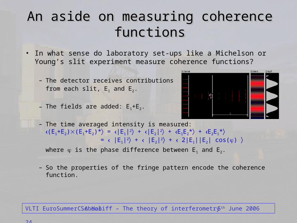
– The detector receives contributionsfrom each slit, E1 and E2.
– The fields are added: E1+E2.
– The time averaged intensity is measured:(E1+E2)(E1+E2)* = |E1|2 + |E2|2 + E1E2* + E2E1*
= |E1|2 + |E2|2 + 2|E1||E2| cos()
where is the phase difference between E1 and E2.
– So the properties of the fringe pattern encode the coherence function.
An aside on measuring coherence functionsAn aside on measuring coherence functionsAn aside on measuring coherence functionsAn aside on measuring coherence functions
• In what sense do laboratory set-ups like a Michelson or Young’s slit experiment measure coherence functions?

VLTI EuroSummer School 255th June 2006C.A.Haniff – The theory of interferometry
Measurements of fringesMeasurements of fringes
• From an interferometric point of view the key features of any interference fringe are its modulation and its location with respect to some reference point.
• In particular we can identify:
[ImaxImin]
[Imax+Imin]V =
– The fringe visibility:
– The fringe phase:• The location of the white-
light fringe as measured fromsome reference (radians).
These measure the amplitude and phase of the complex coherence function, respectively.

VLTI EuroSummer School 265th June 2006C.A.Haniff – The theory of interferometry
A two element interferometer - functionA two element interferometer - function
• Sampling of the radiation (froma distant point source).
• Transport to a common location.
• Compensation for thegeometric delay.
• Combination ofthe beams.
• Detection of theresulting output.
VLTI EuroSummer School 275th June 2006C.A.Haniff – The theory of interferometry
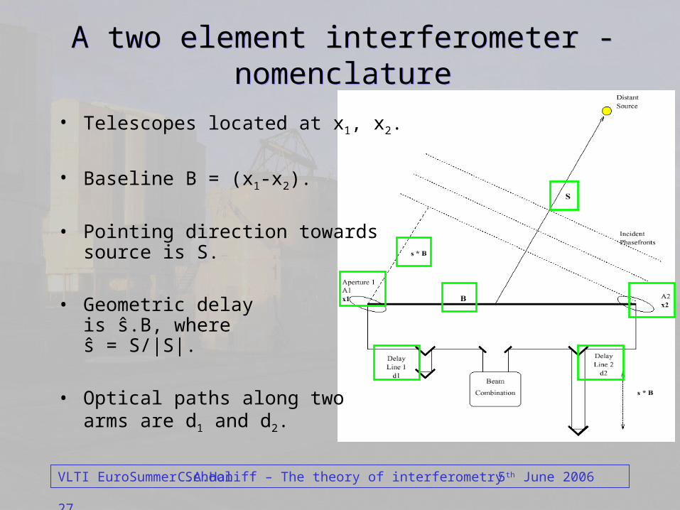
A two element interferometer - nomenclatureA two element interferometer - nomenclature
• Telescopes located at x1, x2.
• Baseline B = (x1-x2).
• Pointing direction towardssource is S.
• Geometric delayis ŝ.B, whereŝ = S/|S|.
• Optical paths along twoarms are d1 and d2.
VLTI EuroSummer School 285th June 2006C.A.Haniff – The theory of interferometry
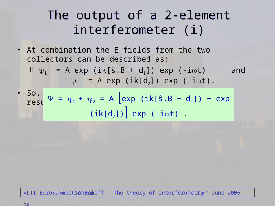
The output of a 2-element interferometer (i)The output of a 2-element interferometer (i)
• At combination the E fields from the two collectors can be described as: 1 = A exp (ik[ŝ.B + d1]) exp (-it) and 2 = A exp
(ik[d2]) exp (-it).
• So, summing these at the detector we get a resultant:
= 1 + 2 = A exp (ik[ŝ.B + d1]) + exp (ik[d2]) exp (-it) .

VLTI EuroSummer School 295th June 2006C.A.Haniff – The theory of interferometry
The output of a 2-element interferometer (i)The output of a 2-element interferometer (i)
• At combination the E fields from the two collectors can be described as: 1 = A exp (ik[ŝ.B + d1]) exp (-it) and 2 = A exp
(ik[d2]) exp (-it).
• So, summing these at the detector we get a resultant:
• Hence the time averaged intensity, *, will be given by:
Note, here D = [ŝ.B + d1 - d2]. This is a function of the path lengths, d1 and d2, the pointing direction (i.e. where the target is) and the baseline.
= 1 + 2 = A exp (ik[ŝ.B + d1]) + exp (ik[d2]) exp (-it) .
* [exp (ik[ŝ.B + d1]) + exp (ik[d2])] [exp (-ik[ŝ.B + d1]) + exp (-ik[d2])]
2 + 2 cos ( k [ŝ.B + d1 - d2] ) 2 + 2 cos (kD)

VLTI EuroSummer School 305th June 2006C.A.Haniff – The theory of interferometry
The output of a 2-element interferometer (ii)The output of a 2-element interferometer (ii)
• The output varies co-sinusiodally with D.
• Adjacent fringe peaksare separated byd1 or 2 = or(ŝ.B) = .
Detected power, P = * 2 + 2 cos (k [ŝ.B + d1 - d2]) 2 + 2 cos (kD), where D = [ŝ.B + d1 - d2]

VLTI EuroSummer School 315th June 2006C.A.Haniff – The theory of interferometry
Extension to polychromatic lightExtension to polychromatic light
• We can integrate the previous result over a range of wavelengths:
– E.g for a uniform bandpass of 0 /2 (i.e. 0 /2) we obtain:
2/
2/
2/
2/
0
0
0
0
)]/2cos(1[2
)]cos(22[
d D
d kDP

VLTI EuroSummer School 325th June 2006C.A.Haniff – The theory of interferometry
Extension to polychromatic lightExtension to polychromatic light
• We can integrate the previous result over a range of wavelengths:
– E.g for a uniform bandpass of 0 /2 (i.e. 0 /2) we obtain:
So, the fringes are modulated with an envelope with a characteristic width equal to the coherence length, coh = 2
0/.
2/
2/
2/
2/
0
0
0
0
)]/2cos(1[2
)]cos(22[
d D
d kDP
DkD
D
DkD
D
coh
coh0
00
2
02
cos /
/sin 1
cos/
/sin 1

VLTI EuroSummer School 335th June 2006C.A.Haniff – The theory of interferometry
Heuristic operation of an interferometerHeuristic operation of an interferometer
• Each unresolved element of the image produces its own fringe pattern.
• These have unit visibility and a phase that is associated with the location of the element in the sky.

VLTI EuroSummer School 345th June 2006C.A.Haniff – The theory of interferometry
Heuristic operation of an interferometerHeuristic operation of an interferometer
• The observed fringe pattern from a distributed source is just the intensity superposition of these individual fringe pattern.
• This relies upon the individual elements of the source being “spatially incoherent”.

VLTI EuroSummer School 355th June 2006C.A.Haniff – The theory of interferometry
Heuristic operation of an interferometerHeuristic operation of an interferometer
• The observed fringe pattern from a distributed source is just the intensity superposition of these individual fringe pattern.
• This relies upon the individual elements of the source being “spatially incoherent”.
VLTI EuroSummer School 365th June 2006C.A.Haniff – The theory of interferometry
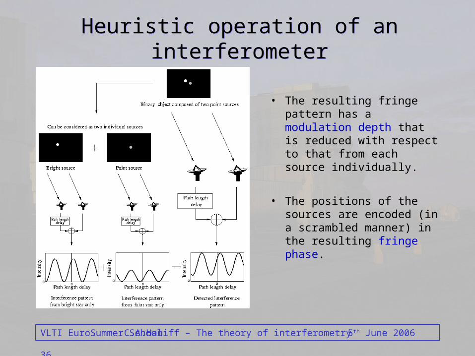
Heuristic operation of an interferometerHeuristic operation of an interferometer
• The resulting fringe pattern has a modulation depth that is reduced with respect to that from each source individually.
• The positions of the sources are encoded (in a scrambled manner) in the resulting fringe phase.

VLTI EuroSummer School 375th June 2006C.A.Haniff – The theory of interferometry
A mathematical interlude A mathematical interlude
• Consider looking at an incoherent source whose brightness on the sky is described by I(ŝ). This can be written as I(ŝ0+s), where ŝ0 is a vector in the pointing direction, and s is a vector perpendicular to this.
• The detected power will be given by:s s0
s
' ).(cos1 )(
)..(cos1 )(
)].([cos1 )(
).(cos1 )(
cos1 )(),(
210
210
21
0
dBsksI
dddBsBsksI
dddBssksI
dddBsksI
dkDsIBsP

VLTI EuroSummer School 385th June 2006C.A.Haniff – The theory of interferometry
Heading towards the van Cittert-Zernike theoremHeading towards the van Cittert-Zernike theorem
• Consider now adding a small path delay, , to one arm of the interferometer. The detected power will become:
' ).(sin)(sin
' ).(cos)(cos ' )(
' ).(cos1 )(),,( 0
dBsksIk
dBsksIkdsI
dBsksIBsP

VLTI EuroSummer School 395th June 2006C.A.Haniff – The theory of interferometry
Heading towards the van Cittert-Zernike theoremHeading towards the van Cittert-Zernike theorem
• Consider now adding a small path delay, , to one arm of the interferometer. The detected power will become:
• We now define something called the complex visibility V(k,B):
so that we can now write the interferometer output as:
' ).(sin)(sin
' ).(cos)(cos ' )(
' ).(cos1 )(),,( 0
dBsksIk
dBsksIkdsI
dBsksIBsP
]Im[sin ]Re[cos' )(),,(
, ' ].exp[)(),(
0 VkVkdsIBsP
dBsiksIBkV
]exp[ Re ),,( 0 ikVIBsP total
VLTI EuroSummer School 405th June 2006C.A.Haniff – The theory of interferometry
What is this V that we introduced?What is this V that we introduced?
• Lets assume ŝ0 = (0,0,1) and s is (,,0), with and small angles measured in radians.
wvu
ddvuiI
ddBBikI
dBsiksIBkV
yx
)](2exp[(
)](exp[(
' ].exp[)(),(

VLTI EuroSummer School 415th June 2006C.A.Haniff – The theory of interferometry
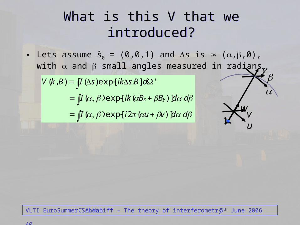
What is this V that we introduced?What is this V that we introduced?
• Lets assume ŝ0 = (0,0,1) and s is (,,0), with and small angles measured in radians.
– Here, u (= Bx/) and v (= By/) are the projections of the baseline onto a plane perpendicular to the pointing direction.
– These co-ordinates have units of rad-1 and are the spatial frequencies associated with the physical baselines.
So, the complex quantity V we introduced is the Fourier Transform of the source brightness distribution.
wvu
ddvuiI
ddBBikI
dBsiksIBkV
yx
)](2exp[(
)](exp[(
' ].exp[)(),(
VLTI EuroSummer School 425th June 2006C.A.Haniff – The theory of interferometry
The bottom lineThe bottom line
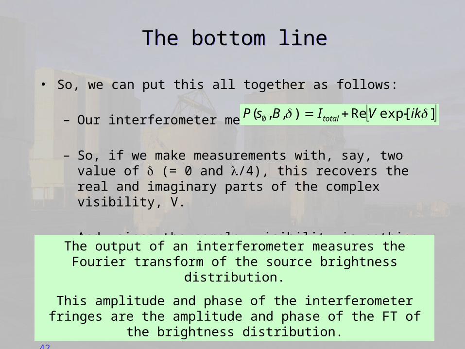
• So, we can put this all together as follows:
– Our interferometer measures:
– So, if we make measurements with, say, two value of (= 0 and /4), this recovers the real and imaginary parts of the complex visibility, V.
– And, since the complex visibility is nothing more than the Fourier transform of the brightness distribution, we have our final results:
]exp[Re ),,( 0 ikVIBsP total
The output of an interferometer measures the Fourier transform of the source brightness distribution.
This amplitude and phase of the interferometer fringes are the amplitude and phase of the FT of the brightness distribution.

VLTI EuroSummer School 435th June 2006C.A.Haniff – The theory of interferometry
TimeoutTimeout
• Image formation with conventional telescopes– The diffraction limit– Incoherent imaging equation– Fourier decomposition
• Coherence functions– Temporal coherence– Spatial coherence
• Interferometric measurements– Fringe parameters– The van-Cittert Zernike theorem
• Imaging with interferometers– Rules of thumb– Interferometric images– Sensitivity

VLTI EuroSummer School 445th June 2006C.A.Haniff – The theory of interferometry
A reality checkA reality check
• How is all this related to the VLTI?
• Telescopes sample the fields at r1 and r2.
• Optical train delivers the radiation to a laboratory.
• Delay lines assure that we measure when t1=t2.
• The instruments mix the beams and detect the fringes.
VLTI EuroSummer School 455th June 2006C.A.Haniff – The theory of interferometry
OutlineOutline
• Image formation with conventional telescopes– The diffraction limit– Incoherent imaging equation– Fourier decomposition
• Coherence functions– Temporal coherence– Spatial coherence
• Interferometric measurements– Fringe parameters– The van-Cittert Zernike theorem
• Imaging with interferometers– Rules of thumb– Interferometric images– Sensitivity
VLTI EuroSummer School 465th June 2006C.A.Haniff – The theory of interferometry
Imaging with interferometersImaging with interferometers
• Physical basis is the van Cittert-Zernike theorem:
– Fourier transform of the brightness distribution is the coherence,
or visibility function, V(u, v) = V(Bx/, By/).
• So in principle the strategy is straightforward:– Measure V for as many values of B as possible.– Perform an inverse Fourier transform image of the source.
• But we need to consider the following topics:– Typical visibility functions - what do they look like?– How complete do the measurement of V(u, v) have to be?– What is the nature of the images that can be recovered?
[Note that all of this will assume the absence of a turbulent atmosphere.]

VLTI EuroSummer School 475th June 2006C.A.Haniff – The theory of interferometry
Simple 1-d sources (i)Simple 1-d sources (i)
V(u) = I(l) ei2(ul) dl I(l) dl
Point source of strength A1 and located at angle l1 relative to the optical axis.
V(u) = A1(l-l1) ei2(ul) dl A1(l-l1)dl
= ei2(ul1)
– The visibility amplitude is unity u.
– The visibility phase varies linearly with u(= B/).
– Sources such as this are easy to observe (the fringes have high contrast),
but are of little interest for imaging purposes.

VLTI EuroSummer School 485th June 2006C.A.Haniff – The theory of interferometry
Simple sources (ii)Simple sources (ii)A double source comprising point sources of strength A1 and A2 located at
angles 0 and l2 relative to the optical axis.
V(u) = [A1(l) + A2(l-l2)] ei2(ul) dl [A1(l) + A2(l-l2)] dl
= [A1+A2ei2(ul2)] [A1+A2]
– The visibility amplitude and phaseoscillate as functions of u.
– To identify this as a binary, baselinesfrom 0 /l2 are required.
– If the ratio of component fluxes is large the modulation of the visibility becomes increasingly difficult to measure.

VLTI EuroSummer School 495th June 2006C.A.Haniff – The theory of interferometry
– The visibility amplitude falls rapidlyas ur increases.
– To identify this as a disc requiresbaselines from 0 / at least.
– Information on scales smaller than the disc diameter correspond to values of ur where V << 1, and is hence difficult to measure.
Simple sources (iii)Simple sources (iii)A uniform on-axis disc source of diameter .
V(ur) /2 J0(2ur) d
= 2J1(ur) (ur)

VLTI EuroSummer School 505th June 2006C.A.Haniff – The theory of interferometry
What can we learn from this?What can we learn from this?
• Distinguishing between different types of sources => measuring fringes for many different baseline lengths.
• The spatial properties of the image are encoded in the different changes in fringe contrast and phase seen as the baseline is altered.
• Point-like targets => fringes that have high contrast, and so are easy to measure.
• Resolved targets => fringes that are difficult to measure.
Understanding the expected values of V is key to designing a useful interferometer.
VLTI EuroSummer School 515th June 2006C.A.Haniff – The theory of interferometry
Imaging with interferometersImaging with interferometers
• In this final section we briefly introduce the essential features of interferometric imaging and touch on the following ideas:
– How the properties of the FT allow for inversion of the interferometer data.
– How the image recovered in this way is related to the true sky brightness distribution.
– How the recovered image can be used to infer the true sky brightness distribution.
– Rules of thumb that you should be aware of.
Note that, for simplicity here, we will assume perfect measurements of the visibility function.
• You will learn later how the effects of noise and the atmosphere are dealt with.
VLTI EuroSummer School 525th June 2006C.A.Haniff – The theory of interferometry
Image reconstructionImage reconstruction
• We start with the fundamental relationship between the visibility function and the normalized sky brightness:
Inorm(l, m) = V(u, v) e+i2(ul + vm) du dv
• In practice what we measure is a sampled version of V(u, v), so the image we have access to is to the so-called “dirty map”:
Idirty(l, m) = S(u, v) V(u, v) e+i2(ul + vm) du dv
= Bdirty(l, m) * Inorm(l, m) ,
where Bdirty(l,m) is the Fourier transform of the sampling distribution, or dirty-
beam.
• The dirty-beam is the interferometer PSF. While it is generally far less attractive than an Airy pattern, it’s shape is completely determined by the samples of the visibility function that are measured.
VLTI EuroSummer School 535th June 2006C.A.Haniff – The theory of interferometry
Deconvolution in interferometryDeconvolution in interferometry
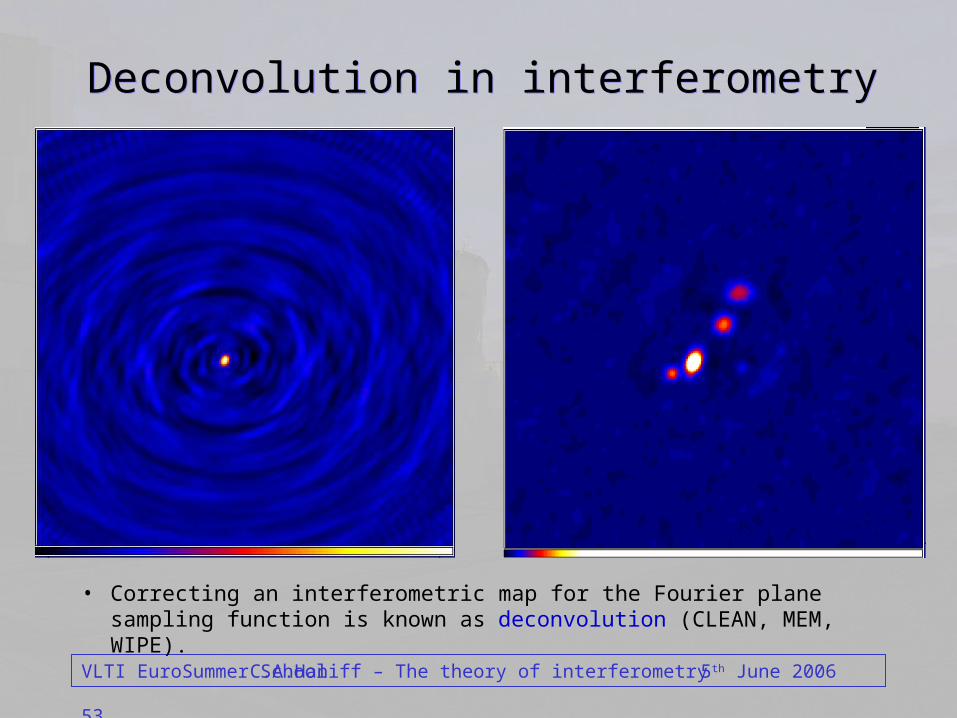
• Correcting an interferometric map for the Fourier plane sampling function is known as deconvolution (CLEAN, MEM, WIPE).

VLTI EuroSummer School 545th June 2006C.A.Haniff – The theory of interferometry
Important rules of thumbImportant rules of thumb
• The number of visibility data number of filled pixels in the recovered image:
– N(N-1)/2 number of reconfigurations number of filled pixels.
• The distribution of samples should be as uniform as possible:– To aid the deconvolution process.
• The range of interferometer baselines, i.e. Bmax/Bmin, will govern the range of spatial scales in the map.
• There is no need to sample the visibility function too finely:
– For a source of maximum extent max, sampling very much finer than u 1/max is unnecessary.

VLTI EuroSummer School 555th June 2006C.A.Haniff – The theory of interferometry
How well is the Fourier plane sampled?How well is the Fourier plane sampled?
• The UV plane shows the vector separations between the interferometer telescopes projected onto a plane perpendicular to the line of sight to the source.
• The figure to the right shows this for anhypothetical 24-element “Keto” array.
• The telescope locations are denoted by the stars,and the baselines (276 in total) by the dots.
• Broadly speaking this gives “uniform” sampling,save for a clustering of baselines near to the origin.
• The main shortcoming is the central hole near the origin.
VLTI EuroSummer School 565th June 2006C.A.Haniff – The theory of interferometry
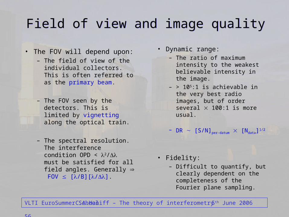
Field of view and image qualityField of view and image quality
• The FOV will depend upon:– The field of view of the
individual collectors. This is often referred to as the primary beam.
– The FOV seen by the detectors. This is limited by vignetting along the optical train.
– The spectral resolution. The interference condition OPD < 2/ must be satisfied for all field angles. Generally FOV [/B][/].
• Dynamic range:– The ratio of maximum intensity
to the weakest believable intensity in the image.
– > 105:1 is achievable in the very best radio images, but of order several 100:1 is more usual.
– DR [S/N]per-datum [Ndata]1/2
• Fidelity:– Difficult to quantify, but clearly
dependent on the completeness of the Fourier plane sampling.

VLTI EuroSummer School 575th June 2006C.A.Haniff – The theory of interferometry
Conventional vs. interferometric imagingConventional vs. interferometric imaging
• Optical HST (left) and 330Mhz VLA (right) images of the Crab Nebula and the Orion nebula. Note the differences in the:
– Range of spatial scales in each image.
– The range of intensities in each image.
– The field of view as measured in resolution elements.

VLTI EuroSummer School 585th June 2006C.A.Haniff – The theory of interferometry
SensitivitySensitivity
• What does this actually mean in an optical/infrared interferometric context?
The “source” has to be bright enough to:
– Allow stabilisation of the interferometric path lengths in real time.
– Allow a reasonable signal-to-noise for the fringe parameters to be build up over some total convenient integration time. This will be measured in minutes.
– Once this achieved, the faintest features in the interferometric map will be governed by the dynamic range achievable:
• This in turn depends on the S/N and number of visibility data.
VLTI EuroSummer School 595th June 2006C.A.Haniff – The theory of interferometry
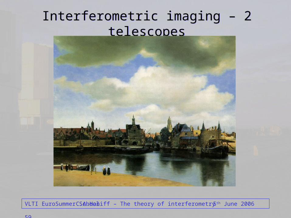
Interferometric imaging – 2 telescopesInterferometric imaging – 2 telescopes

VLTI EuroSummer School 605th June 2006C.A.Haniff – The theory of interferometry
Interferometric imaging – 2 telescopesInterferometric imaging – 2 telescopes
VLTI EuroSummer School 615th June 2006C.A.Haniff – The theory of interferometry
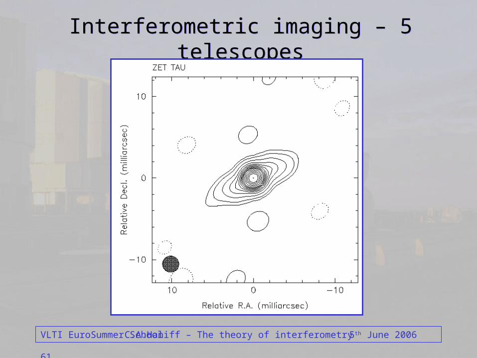
Interferometric imaging – 5 telescopesInterferometric imaging – 5 telescopes

VLTI EuroSummer School 625th June 2006C.A.Haniff – The theory of interferometry
Interferometric imaging – 21 telescopesInterferometric imaging – 21 telescopes

VLTI EuroSummer School 635th June 2006C.A.Haniff – The theory of interferometry
Interferometric imaging resumeInterferometric imaging resume
• 2 telescopes: simple parametric model fitting.
• 5 telescopes: rudimentary imaging of astronomical sources.
• 21 telescopes: imaging of complex astrophysical phenomena.

VLTI EuroSummer School 645th June 2006C.A.Haniff – The theory of interferometry
SummarySummary
• Image formation with conventional telescopes:– Fourier decomposition, spatial frequencies, physical baselines.
• Coherence functions:– Spatial & temporal: these embody the spatial & spectral content of the
source.
– Fundamental relationships are Fourier transforms.
• Interferometric measurements:– Fringe amplitude and phase are what is important.
– Ability to measure these depends on signal strength & fringe modulation.
• Imaging with interferometers:– Rules of thumb and differences with respect to what we are used to.
– Expectations based on 50 years of radio/optical/infrared experience.