An introduction to Symanzik's O(a) improvement programme

An introduction to Symanzik’s O(a) improvementprogramme

Stefan Sint

Trinity College Dublin

STRONGnet Summer School 2011

Bielefeld, 14 June 2011

Stefan Sint An introduction to Symanzik’s O(a) improvement programme 1 / 27

Contents

1 Non-perturbative definition of QCD

2 Renormalisation of QCD with Wilson quarks

3 Symanzik’s effective continuum theory

4 Symanzik O(a) improvement

5 Non-perturbative determination of improvement coefficients

6 Some results

7 A warning from 2 dimensions

8 Conclusions


Non-perturbative definition of QCD (1)

To define QCD as a QFT it is not enough to write down its classicalLagrangian:

LQCD(x) =1

2g2tr {Fµν(x)Fµν(x)}+

Nf∑i=1

ψi (x) (D/+ mi )ψi (x)

One needs to define the functional integral:

Introduce a Euclidean space-time lattice and discretise the continuumaction such that the doubling problem is solved

Consider a finite space-time volume ⇒ the functional integralbecomes a finite dimensional ordinary or Grassmann integral, i.e.mathematically well defined!

Take the infinite volume limit L→∞Take the continuum limit a→ 0



In massive theories the infinite volume limit is reached withexponential corrections ⇒ not a major problem in practice.

Continuum limit: existence only established order by order inperturbation theory & only for selected lattice regularisations:

lattice QCD with Wilson quarks [Reisz ’89 ]lattice QCD with overlap/Neuberger quarks [Reisz, Rothe ’99 ]not (yet ?) for lattice QCD with staggered quarks [cf. Giedt ’06 ]

From asymptotic freedom expect

g20 = g2

0 (a)a→0∼ −1

2b0 ln a, b0 = 11N

3 −23Nf



Working hypothesis: the perturbative picture is essentially correct:

The continuum limit of lattice QCD exists and is obtained by takingg0 → 0

Hence, QCD is asymptotically free, naive dimensional analysis applies:non-perturbative renormalisation of QCD is based on the very samecounterterm structure as in perturbation theory!

Absence of analytical methods: try to take the continuum limitnumerically, i.e. by numerical simulations of lattice QCD atdecreasing values of g0.

Typical current ranges for a:

a = 0.04− 0.1 fm

i.e. at most a variation by a factor 2-3!


Renormalisation of QCD

The basic parameters of QCD are g0 and mi , i = u, d , s, c , b, t.

To renormalise QCD one must impose a corresponding number ofrenormalisation conditions

We only consider gauge invariant observables ⇒ no need to considerfield renormalisations for quark, gluon or ghost fields or therenormalisation of the gauge parameter.

All physical information (particle masses and energies, particleinteractions) is contained in the (Euclidean) correlation functions ofgauge invariant composite, local fields φi (x)

〈φ1(x1) · · ·φn(xn)〉

a priori each field φi requires renormalisation, and thus furtherrenormalisation conditions.


Counterterm structure in lattice QCD with Wilson quarks

The action S = Sf + Sg is given by

Sf = a4∑x

ψ(x) (DW + m0)ψ(x), Sg = 1g2

0

∑µ,ν

tr {1− Pµν(x)}

DW = 12

{(∇µ +∇∗µ

)γµ − a∇∗µ∇µ

}Symmetries: U(Nf)V (mass degenerate quarks), P,C ,T and O(4,ZZ)

⇒ Renormalized parameters:

g2R = Zgg2

0 , mR = Zm (m0 −mcr) , amcr = amcr(g0).

In general: Z = Z (g0, aµ, am0);

Quark mass independent renormalisation schemes: Z = Z (g0, aµ)

Simple non-singlet composite fields, e.g. Pa = ψγ512τ

aψ renormalisemultiplicatively, Pa

R = ZP(g0, aµ, am0)Pa


Symanzik’s effective continuum theory (1) [Symanzik ’79 ]

goal: render the a-dependence of lattice correlation functions explicit.⇒ structural insight into the nature of cutoff effects

at scales far below the cutoff a−1, the lattice theory is effectivelycontinuum-like and can be represented by an effective continuumtheory, with action

Seff = S0 + aS1 + a2S2 + . . . , S0 = ScontQCD

Sk =

∫d4x Lk(x)

Lk(x): linear combination of fields

with canonical dimension 4 + kwhich share all the symmetries with the lattice action


Symanzik’s effective continuum theory (2)

The first term L1 can be parametrized by:

L1 = c(1)1 ψσµνFµνψ+c

(2)1 ψD2ψ+c

(3)1 mψD/ψ+c

(4)1 m2ψψ+c

(5)1 m tr {FµνFµν}

The same procedure applies to composite fields:

φeff(x) = φ0 + aφ1 + a2φ2 . . .

for instance: φ(x) = Pa(x):

Paeff = ψγ5

12τ

aψ + c(1)P mψγ5

12τ

aψ + c(2)P

(ψD/←γ5

12τ

aψ − ψγ512τ

aD/ψ)

Consider renormalised, connected lattice n-point functions of amultiplicatively renormalisable field φ

Gn(x1, . . . , xn) = Znφ 〈φ(x1) · · ·φ(xn)〉latcon



Effective field theory description:

Gn(x1, . . . , xn) = 〈φ0(x1) . . . φ0(xn)〉con

+ a

∫d4y 〈φ0(x1) . . . φ0(xn)L1(y)〉con

+ an∑

k=1

〈φ0(x1) . . . φ1(xk) . . . φ0(xn)〉con + O(a2)

〈· · · 〉 is defined w.r.t. continuum theory with S0

the a-dependence is now explicit, up to logarithms, which are hiddenin the coefficients c1,i andIn perturbation theory one expects to l-loop order the asymptoticexpansion:

P(a) ∼ P(0) +∞∑

n=1

l∑k=0

g2k0 pnkan(ln a)k

where e.g. P(a) = Gn at fixed arguments.Stefan Sint An introduction to Symanzik’s O(a) improvement programme 10 / 27


Conclusions from Symanzik’s analysis:

Asymptotically, cutoff effects are powers in a, modified by logarithms;

In contrast to Wilson quarks, only even powers of a are expected for

4-dim. bosonic theories (pure gauge theories, scalar field theories)4-dim. fermionic theories which retain a remnant axial symmetry(overlap, Domain Wall Quarks, staggered quarks, Wilson quarks with atwisted mass term,...)

In QCD simulations a is typically varied by a factor 2

⇒ logarithms vary too slowly to be resolved; linear or quadratic fits (in aresp. a2) are used in practice.


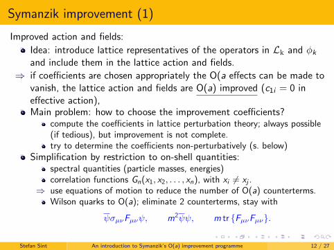
Symanzik improvement (1)

Improved action and fields:

Idea: introduce lattice representatives of the operators in Lk and φk

and include them in the lattice action and fields.

⇒ if coefficients are chosen appropriately the O(a effects can be made tovanish, the lattice action and fields are O(a) improved (c1i = 0 ineffective action),Main problem: how to choose the improvement coefficients?

compute the coefficients in lattice perturbation theory; always possible(if tedious), but improvement is not complete.try to determine the coefficients non-perturbatively (s. below)

Simplification by restriction to on-shell quantities:spectral quantities (particle masses, energies)correlation functions Gn(x1, x2, . . . , xn), with xi 6= xj .

⇒ use equations of motion to reduce the number of O(a) counterterms.Wilson quarks to O(a); eliminate 2 counterterms, stay with

ψσµνFµνψ, m2ψψ, m tr {FµνFµν}.


Symanzik improvement (2)

1 On-shell O(a) improved lattice QCD actionThe last two terms are equivalent to a rescaling of the bare mass andcoupling (mq = m0 −mcr):

g20 = g2

0 (1 + bg (g0)amq), mq = mq(1 + bm(g0)amq)

The only new structure is the Sheikholeslami-Wohlert or clover term

SWilson → SWilson + i4acsw(g2

0 )a4∑

x

ψ(x)σµν Fµν(x)ψ(x)

2 On-shell O(a) improved axial current and density:

(AR)aµ = ZA(g0

2)(1 + bA(g0)amq){

Aaµ + cA(g0)∂µP

a}

(PR)a = ZP(g02, aµ)(1 + bP(g0)amq)Pa


Determination of improvement coefficients

In principle determine O(a) improvement coefficients non-perturbatively asfunctions of g2

0 by imposing (i = 1, 2, . . .)

Pi (a; csw, cA, . . .) = Pi (0), ⇒ csw(g20 ), cA(g2

0 ) . . .

problem: requires knowledge of the very continuum results Pi (0)which O(a) improvement should help to obtain!

can be done in perturbation theory

Observation: O(a) counterterms with Wilson fermions arise due toexplicit breaking of chiral symmetry!

⇒ can be determined by imposing chiral symmetry relations at finitelattice spacing (i.e. fixed g0).


Improvement conditions from chiral symmetry

In QFT symmetries are expressed by Ward identities

introduce axial field variations:

δaA(θ)ψ(x) = iγ512τ

aθ(x)ψ(x), δaA(θ)ψ(x) = ψ(x)iγ512τ

aθ(x)

with θ(x) = 1 if x ∈ R and = 0 otherwise (R = space-time region)

Derive continuum Ward identities by assuming that the functionalintegral can be treated like an ordinary integral:

〈δaA(θ)O〉 = 〈OδaA(θ)S〉,

δaA(θ)S = −i

∫d4xθ(x)

(∂µA

aµ(x)− 2mPa(x)

)Aaµ(x) = ψ(x)γµγ5

12τ

aψ(x), Pa(x) = ψ(x)γ512τ

aψ(x)


Simplest chiral Ward identity: the PCAC relation

Choose fields O = Oext located outside region R, then shrink R to apoint x :

0 = 〈OextδaA(θ)S〉 = −i

⟨Oext

(∂µA

aµ(x)− 2mPa(x)

)⟩,

Rewritten in terms of the PCAC mass:

m =〈Oext∂µA

aµ(x)〉

2〈OextPa(x)〉

NOTE: chiral symmetry implies that the PCAC mass must beindependent of

the choice of Oext,the point x orany other parameters such as the space-time volume or shape!


Non-perturbative determination of csw

There are 2 improvement coefficients in the massless theory (csw, cA),the remaining ones (bg , bm, bA, bP) come with amq.

All counterterms are absent in chirally symmetric regularisations⇒ turn this around: impose chiral symmetry to determine csw, cA

non-perturbatively:define bare PCAC quark masses from SF correlation functions(i.e. choice of Oext etc.):

mR =ZA(1 + bAamq)

ZP(1 + bPamq)m, m =

∂0fA(x0) + cAa∂∗0∂0fP(x0)

fP(x0)

At fixed g0 and amq ≈ 0 define 3 bare PCAC masses m1,2,3 (e.g. byvarying the gauge boundary conditions) and impose

m1(csw, cA) = m2(csw, cA), m1(csw, cA) = m3(csw, cA)⇒ csw, cA

SF b.c.’s ⇒ high sensitivity to csw & simulations near chiral limit


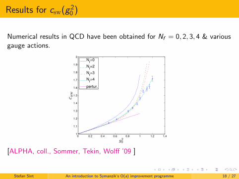
Results for csw(g 20 )

Numerical results in QCD have been obtained for Nf = 0, 2, 3, 4 & variousgauge actions.

0 0.2 0.4 0.6 0.8 1 1.2 1.41

1.1

1.2

1.3

1.4

1.5

1.6

1.7

1.8

1.9

2

g20

c sw

Nf=0

Nf=2

Nf=3

Nf=4

pertur.

[ALPHA, coll., Sommer, Tekin, Wolff ’09 ]


Effect of on-shell O(a) improvement

Before and after O(a) improvement (PCAC masses from SF correlationfunctions, 83 × 16 lattice)


Quenched result for the charm quark mass [ALPHA ’02 ]

The RGI charm quark mass can be defined in various waysstarting from the subtracted bare quark mass mq,c = m0,c −mcr

starting from the average strange-charm PCAC mass msc

starting from the PCAC mass mcc for a hypothetical mass degeneratedoublet of quarks.

Tune the bare charm quark masses to match the Ds meson mass

Obtain the corresponding O(a) improved RGI masses:

r0Mc |msc = ZM

{2r0msc

[1 + (bA − bP)1

2(amq,c + amq,s)]

− r0ms [1 + (bA − bP)amq,s)]},

r0Mc |mc = ZM r0mc [1 + (bA − bP)amq,c] ,

r0Mc |mq,c = ZMZr0mq,c [1 + bmamq,c] .

N.B.: all O(a) counterterms are known non-perturbatively in thequenched case!


Continuum extrapolation of the quenched RGI charmquark mass

Continuum extrapolation:

r0Mc = A + B(a2/r20 )

r0 = 0.5 fm

Mc = 1.654(45) GeV

mMSc (mc) = 1.301(34) GeV


Continuum extrapolation of FDsin quenched QCD

[Heitger, Juttner ’08 ]

0 0.01 0.02 0.030.5

0.55

0.6

0.65

0.7this work cA by ALPHA [20]

Ali-Khan et al. [2]this work cA by LANL [21]

(a/r0)2

r 0F

Ds

0 0.01 0.02 0.030.91

1.11.21.31.4

0 0.01 0.02 0.030.25

0.3

0.35

Warning: if a is not small enough the continuum extrapolations can bemisguided!


The 2d O(N) sigma model: a test laboratory for QCD?

S =1

g20

∑x ,µ

(∂µS)2, S = (S1, . . . ,SN) S2 = 1

like QCD the model has a mass gap and is asymptotically free

many analytical tools: large N expansion, Bethe ansatz, form factorbootstrap;

some exact results available in continuum limit!

efficient numerical simulations due to cluster algorithms.

⇒ very precise data over a wide range of lattice spacing (a can be variedby 1-2 orders of magnitude).

Symanzik: expect O(a2) effects, up to logarithms!


A sobering result:

Numerical study of renormalised finite volume coupling to high precision(N = 3) [Hasenfratz, Niedermayer ’00, Hasenbusch et al. ’01, Balog,Niedermayer, Weisz ’09 ]

0 0.05 0.1a/L

0

0.01

0.02

0.03

0.04

δΣ(2

,u0,a

/L)

O(3), STO(3), D(1/3)O(3), D(-1/4)

Cutoff effects seem to be almost linear in a!Is this just an unfortunate case?


A closer look:

[Balog, Niedermayer, Weisz ’09 ] cutoff effects ×L2/a2:

1.8 1.9 2 2.1β

eff

0

5

10

15

20

δ∆(2

,u0,a

/L)*

(L/a

)2

1.5 1.6 1.7 1.8 1.9β

eff

0

2

4

6

8

δ∆(2

,u0,a

/L)*

(L/a

)2

Cuprit: terms like a2 ln3(a2) conspire to fake a linear behaviour in a overwide range! However, can be understood within Symanzik’s effectivetheory!


O(a2) effects in lattice QCD

L2 contains a host of dimension 6 operators (4-quark operators!)[Sheikholeslami-Wohlert ’86 ]

⇒ complete elimination of O(a2) effects in lattice QCD a la Symanzik isunpractical!

Pure gauge theories: O(a2) terms can be eliminated by adding moreextended Wilson loops to the Wilson plaquette action [Luscher, Weisz’84 ]; in QCD this is sometimes done for other reasons than O(a2)improvement.

O(a) improvement for Wilson quarks gets complicated

if quarks are not mass-degeneratefor 4-quark operators due to proliferation of O(a) counterterms.

⇒ introduce “twisted mass terms” [Frezzotti, Grassi, S. Weisz, ’01 ] andrely on “automatic O(a) improvement” [Frezzotti, Rossi ’03 ].


Conclusions

Symanzik’s analysis seems applicable beyond perturbation theory;cutoff effects are organized powers of a up to (slowly varying)logarithms

In lattice QCD numerical results seem to confirm expectations;

However, large powers of logarithms are a possibility (cf. O(3) model)and could be problematic!

While Symanzik’s effective theory allows to unveal this behaviour, thecalculations are tedious! [Balog, Niedermayer, Weisz ’09 ]

Improvement coefficients are difficult determine non-perturbatively,except where continuum symmetries are broken (e.g chiral symmetrywith Wilson quarks)

Perturbative determinations: automated perturbative methods orstochastic perturbation theory might enable two-loop results whichmay be sufficient in many cases.


An introduction to Symanzik's O(a) improvement programme

Documents

Transcript of An introduction to Symanzik's O(a) improvement programme