An Introduction to Multiple Time Series Analysis and the VARMAX … · 2000-01-01 · An...

1

SAS4306-2020

An Introduction to Multiple Time Series Analysis and the

VARMAX Procedure

Xilong Chen, SAS Institute Inc.

ABSTRACT

To understand the past, update the present, and forecast the future of a time series, you

must often use information from other time series. This is why simultaneously modeling

multiple time series plays a critical role in many fields. This paper shows how easy it is to

use the VARMAX procedure to estimate and interpret several popular and powerful

multivariate time series models, including the vector autoregressive (VAR) model, the

vector error correction model (VECM), and the multivariate GARCH model. Simple examples

illustrate Granger causality tests for identifying predictive causality, impulse response

analysis for finding the effect of shocks, cointegration and its importance in forecasting,

model selection for dealing with the trade-off between bias and variance, and volatility

forecasting for risk management and portfolio optimization.

INTRODUCTION

When you analyze a time series, the type of analysis you use usually depends on the nature

of the time series: When a time series’ current value depends on its past values, you might

use autoregression (AR). When current values in a vector of multiple time series depend on

their past values and even on each other’s current values, you might use vector

autoregression (VAR), which systemically captures the dynamics in multiple time series.

When long-run equilibrium exists between multiple nonstationary time series, you might use

a vector error correction model (VECM) to exploit both the long-run and short-run

relationships. When you need to forecast volatility, which is very important in risk

management and portfolio optimization, you might use an autoregressive conditional

heteroscedasticity (ARCH) or a generalized autoregressive conditional heteroscedasticity

(GARCH) model. These models are often used in modeling and forecasting volatility for both

univariate and multivariate cases.

The next three sections show examples of some of the models you can use. The first is a

simple VAR example that illustrates Granger causality tests for identifying predictive

causality, impulse response analysis for finding the effect of shocks, and model selection for

dealing with the trade-off between bias and variance. The second example shows how to

incorporate the concept of purchasing power parity (PPP) in a VECM and then how well it

leads to some good forecasts. The third example applies a multivariate dynamic conditional

correlation (DCC) GARCH model on Japanese and US stock market returns and then uses

the forecasted volatility in portfolio optimization to achieve a trading strategy that has a

better long-run return and return per risk unit than three other benchmark trading

strategies.

VECTOR AUTOREGRESSIVE MODEL

Since Sims1 (1980) introduced the VAR model into macroeconomic econometrics, it has

been widely used in forecasting and policy analysis. This section uses simulated data on

1 Christopher Sims and Thomas Sargent were awarded a Nobel Prize in 2011 “for their empirical research on cause and effect in the macroeconomy” (Nobel Media AB 2020b).

2

inflation, unemployment rate, and interest rate to discuss some basic concepts of using a

VAR model, namely Granger causality tests, impulse response functions, and model

selection. For a real-data example and further discussion of the advantages and

disadvantages of VAR models, see Stock and Watson (2001).

The following statements read the simulated data and plot three time series, which are

shown in Figure 1:

data simul1;

input date mmddyy10. inflation interestRate unemploymentRate;

format date yyq.;

datalines;

01/01/1950 10.0088 11.9544 5.28514

04/01/1950 11.3452 12.7174 5.45672

... more lines ...

07/01/1999 9.1981 11.6830 5.02263

10/01/1999 10.6646 13.0948 4.57442

;

proc sgplot data=simul1;

series x=date y=inflation / legendlabel="Inflation";

series x=date y=unemploymentRate / legendlabel="Unemployment Rate";

series x=date y=interestRate / legendlabel="Interest Rate";

yaxis label="Time Series"; xaxis label="Date";

run;

Figure 1. Plot of Three Time Series

It might be difficult to tell how these three time series affect each other from Figure 1. You

can use the VARMAX procedure to estimate a VAR model in order to find out whether a

relationship exists among these three time series.

3

MODEL SELECTION OF AR ORDER

How to select the AR order in a VAR model is the first important question for model

selection. You can use the MINIC= option in the VARMAX procedure to help you answer this

question, as in the following statements, which also use the DATA=(WHERE=) option to

base the VAR model on the data before 1998. (Using the data before 1998 to estimate the

model leaves the last eight quarters of data as out-of-sample data.)

proc varmax data=simul1(where=(date<'01JAN1998'd));

id date interval=quarter;

model inflation unemploymentRate interestRate /

minic=(type=aicc p=5 q=0);

run;

Notice that the P= option (which specifies the AR order) is not directly specified in the

MODEL statement. Instead, the MINIC= option in the MODEL statement includes the P=5

suboption, which requests that the information criterion specified in the TYPE= suboption be

calculated for orders 0 through 5. As shown in Figure 2, the AR 4 row corresponds to the

smallest AICC, which indicates that 4 should be the selected AR order. In the analysis in the

next section, P=4 is explicitly specified as an option in the MODEL statement.

Figure 2. Minimum Information Criterion Based on AICC

GRANGER CAUSALITY TESTS AND IMPULSE RESPONSE FUNCTIONS

The following statements perform the Granger causality tests and plot the impulse response

functions:

proc varmax data=simul1(where=(date<'01JAN1998'd)) plots=all;


model inflation unemploymentRate interestRate / p=4 lagmax=24;

causal group1=(inflation) group2=(unemploymentRate);

causal group1=(inflation) group2=(interestRate);

causal group1=(unemploymentRate) group2=(inflation);

causal group1=(unemploymentRate) group2=(interestRate);

causal group1=(interestRate) group2=(inflation);

causal group1=(interestRate) group2=(unemploymentRate);

run;

4

In the preceding statements, each of six CAUSAL statements checks the Granger causality

between two variables (that is, whether the variable listed in the GROUP2= option

contributes to the forecast variable listed in the GROUP1= option). The testing result is

shown in Figure 3. The p-values shown in the “Pr > ChiSq” column clearly indicate that

unemployment rate Granger-causes both inflation and interest rate at the 5% significance

level, but neither inflation nor interest rate Granger-causes unemployment rate at the 5%

significance level. From this view, unemployment rate can even be treated as an exogenous

variable and then moved to the right-hand side of the equation, which is beyond the scope

of this paper.

Figure 3. Granger Causality Tests

The PLOTS=ALL and LAGMAX=24 options in the preceding statements request all plots of

three types of impulse response functions (IRFs)—namely standard, accumulated, and

orthogonalized IRFs—in 24 lags. Figure 4 shows the impact of an inflation shock (impulse)

on three variables over time: inflation’s response decreases over time, unemployment rate

has almost no response, and interest rate’s response increases in the first three years and

then decreases at a very slow rate. Be cautious about these IRFs, which are based on

simulated data rather than on real data.

5

Figure 4. Impulse Response Functions

RESTRICTED VAR MODEL

Because the Granger causality tests show that past values of inflation and interest rate are

not likely to help forecast unemployment rate, a better model might be achieved by

restricting those parameters to be 0 in order to exclude them from the model. The restricted

VAR(4) model is estimated by using the RESTRICT statement, as follows:



model inflation unemploymentRate interestRate / p=4;

output out=o11 lead=8;

restrict ar(1:4,unemploymentRate,inflation)=0,

ar(1:4,unemploymentRate,interestRate)=0;

run;

As shown in Figure 5, although the restricted VAR(4) model has a smaller log likelihood than

the former VAR(4) model (in the section “Granger Causality Tests and Impulse Response

Functions”), the restricted VAR(4) model also has a smaller AICC than the former VAR(4)

model, which implies that the restricted VAR(4) is likely to be a better model for out-of-

sample forecasting.

6

Figure 5. Comparison between VAR (Left) and Restricted VAR (Right) Models

The following statements plot the eight-quarter out-of-sample forecasts and their

confidence intervals together with the actual values. The plot is shown in Figure 6.

data o12;

set o11(where=(date>='01JAN1998'd));

set simul1(where=(date>='01JAN1998'd));

id = 1; name = "Inflation ";

actual = inflation; forecast = for1;

lci = lci1; uci = uci1; output;

id = 2; name = "Unemployment Rate";

actual = unemploymentRate; forecast = for2;


id = 3; name = "Interest Rate ";

actual = interestRate; forecast = for3;


keep id name date actual forecast lci uci;

run;

proc sort data=o12; by id; run;

proc sgpanel data=o12;

panelby name / layout=rowlattice uniscale=column novarname sort=data;

band x=date upper=uci lower=lci / legendlabel="Confidence Interval";

series x=date y=forecast / legendlabel="Forecast";

scatter x=date y=actual / legendlabel="Actual Value";

rowaxis display=(nolabel);

colaxis label="Date" type=time interval=quarter;

run;

7

Figure 6. Out-of-Sample Forecasts of Three Time Series and Their Actual Values

VECTOR ERROR CORRECTION MODEL

When some nontrivial linear combination of two or more nonstationary time series leads to

a stationary time series, these nonstationary time series are called cointegrated. The

cointegration, sometimes also called common trends, is very important in modeling

nonstationary time series. Clive Granger was awarded a Nobel Prize in 2003 “for methods of

analyzing economic time series with common trends (cointegration)” (Nobel Media AB

2020a). The main tool for modeling cointegration is the vector error correction model

(VECM), which exploits both the long-run equilibrium and short-run relationships in the

nonstationary time series. One popular example is the relationship between exchange rates

and price indices (which are both nonstationary time series). According to the concept of

purchasing power parity (PPP), the ratio between exchange rate and price index should be a

constant at long-run equilibrium. In this section, simulated data mimic the exchange rate

between the British pound and the US dollar and the price index of the UK as a relative price

versus the US.

8

The following statements read the simulated data of the exchange rate and price index and

then generate their natural logarithm values for further modeling:

data simul2;

input xr p;

date=intnx('year', '01jan1950'd, _n_-1 ); format date year.;

lp = log(p); lx = log(xr);

datalines;

0.38972 62.941

0.38961 63.445

... more lines ...

0.59267 134.171

0.54500 144.752

;

The following statements estimate the VECM model on data before 2000 (which leaves eight

years of data from 2000 to 2007 as out-of-sample data):


id date interval=year;

model lp lx / p=2;

cointeg rank=1 ectrend normalize=lx;

output out=o21 lead=8;

run;

The estimation result of long-run parameters, as shown in Figure 7, indicates that the

difference between the logarithm of the exchange rate and the logarithm of the price index

are close to some constant, which confirms the economic theory.

Figure 7. Long-Run Parameter Estimates

9

The following statements plot the out-of-sample forecasts together with their actual values.

The plots are shown in Figure 8 and Figure 9.

data o22;

set o21(where=(date>='01JAN2000'd));

set simul2(where=(date>='01JAN2000'd));

run;

proc sgplot data=o22;

band x=date lower=lci1 upper=uci1 / legendlabel="Confidence Interval";

series x=date y=for1 / legendlabel="Forecast";

scatter x=date y=lp / legendlabel="Actual Value";

yaxis label="log(Price Index)"; xaxis label="Date";

run;


band x=date lower=lci2 upper=uci2 / legendlabel="Confidence Interval";

series x=date y=for2 / legendlabel="Forecast";

scatter x=date y=lx / legendlabel="Actual Value";

yaxis label="log(Exchange Rate)"; xaxis label="Date";

run;

As shown in Figure 8 and Figure 9, the forecasts are very good. For further discussion about

VECMs and their model selection, see Chen and Kechagias (2017).

Figure 8. Out-of-Sample Forecasts of Log Price Index and Their Actual Values

10

Figure 9. Out-of-Sample Forecasts of Log Exchange Rate and Their Actual Values

MULTIVARIATE GARCH MODEL

Time-varying volatility and volatility clustering, which are common in financial time series,

play an important role in risk management, portfolio optimization, and other fields. Robert

Engle was awarded a Nobel Prize in 2003 “for methods of analyzing economic time series

with time-varying volatility (ARCH)” (Nobel Media AB 2020a). The ARCH and GARCH models

have been widely used in volatility modeling and forecasting. This section models simulated

data for the Japanese and US stock market weekly returns by using a DCC-GARCH model,

and then uses the forecasted volatility in the portfolio optimization to generate a trading

strategy that is far better than three benchmark trading strategies.

The following statements read simulated data and plot the Japanese and US stock market

weekly returns in Figure 10:

data simul3;

input date mmddyy10. jpWeeklyReturn usWeeklyReturn;

format date mmddyy10.;

datalines;

01/13/1965 1.8863 1.4196

01/21/1965 -0.8785 0.7890

... more lines ...

12/17/2019 2.7634 1.8973

12/24/2019 -0.9835 0.9620

;


series x=date y=jpWeeklyReturn;

yaxis label="Japanese Stock Market Weekly Return"; xaxis label="Date";

run;

11


series x=date y=usWeeklyReturn;

yaxis label="US Stock Market Weekly Return";

xaxis label="Date";

run;

Figure 10. Japanese and US Stock Market Weekly Returns

In the VARMAX procedure, you can use the GARCH statement to specify a multivariate

GARCH model. The FORM=DCC option specifies the dynamic conditional correlation (DCC)

GARCH model. The SUBFORM=GJR option together with P=1 and Q=1 options specify the

GJR GARCH(1,1) model for each time series in order to address the asymmetric news

impact: negative and positive shocks of the same magnitude have different effects on future

volatility. The OUTHT= option specifies the output table for the forecasted volatility. The

TECH=TR option in the NLOPTIONS statement is used to specify the trust region

optimization algorithm, which leads to the correct estimation in this example.

ods output GARCHParameterEstimates = ogarchparm31 CovInnovation=ocov31;

proc varmax data=simul3;

model jpWeeklyReturn usWeeklyReturn;

garch form=dcc p=1 q=1 subform=gjr outht=oh31;

nloptions tech=tr;

run;

The GARCH model parameter estimation result (as shown in Figure 11) indicates that all

parameters are significant at the 5% significance level, which means that the conditional

correlation is likely to be time-varying (DCC vs. CCC) and that the news impact is

asymmetric (GJR GARCH vs. standard GARCH).

12

Figure 11. GARCH Model Parameter Estimates

The following statements plot the conditional correlation against time in Figure 12 and plot

the news impact curves for the Japanese and US stock markets in Figure 13:

data oh32; set oh31; set simul3; corr = h1_2 / sqrt(h1_1*h2_2); run;

proc sgplot data=oh32;

series x=date y=corr;

yaxis max=1 label="Correlation"; xaxis label="Date";

run;

proc iml;

use ogarchparm31; read all var {estimate} into garchParm; close;

use ocov31; read all into cov; close;

omega1 = garchParm[4]; alpha1 = garchParm[6]; gamma1 = garchParm[8];

beta1 = garchParm[10]; sigma1 = cov[1,1];

omega2 = garchParm[5]; alpha2 = garchParm[7]; gamma2 = garchParm[9];

beta2 = garchParm[11]; sigma2 = cov[2,2];

eps = (-100:100)`/10; h1=J(nrow(eps),1,0); h2=J(nrow(eps),1,0);

do i = 1 to nrow(eps);

if(eps[i]<0) then h1[i] = omega1 + beta1*sigma1

+ (alpha1+gamma1)*eps[i]*eps[i];

else h1[i] = omega1 + beta1*sigma1 + (alpha1)*eps[i]*eps[i];

if(eps[i]<0) then h2[i] = omega2 + beta2*sigma2

+ (alpha2+gamma2)*eps[i]*eps[i];

else h2[i] = omega2 + beta2*sigma2 + (alpha2)*eps[i]*eps[i];

end;

epsh = eps || h1 || h2;

cn = {'eps' 'jpH' 'usH'};

create o33 from epsh[colname=cn]; append from epsh; close;

quit;

13


styleattrs datacontrastcolors=(black blue);

scatter x=eps y=jpH / legendlabel="JP";

scatter x=eps y=usH / legendlabel="US";

refline 0 / axis=x lineattrs=(color=gray thickness=2);

refline 0 / axis=y lineattrs=(color=gray thickness=2);

yaxis label="Current Volatility" min=0;

xaxis label="Previous Return Shock";

run;

Figure 12. Dynamic Conditional Correlations between Japanese and US Stock Market Returns

14

Figure 13. News Impact Curves for Japanese and US Stock Markets

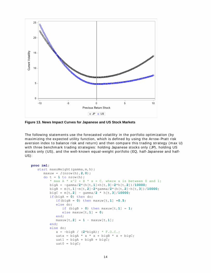
The following statements use the forecasted volatility in the portfolio optimization (by

maximizing the expected utility function, which is defined by using the Arrow-Pratt risk

aversion index to balance risk and return) and then compare this trading strategy (max U)

with three benchmark trading strategies: holding Japanese stocks only (JP), holding US

stocks only (US), and the well-known equal-weight portfolio (EQ, half-Japanese and half-

US):

proc iml;

start maxuWeight(gamma,m,h);

maxuw = J(nrow(h),2,0);

do t = 1 to nrow(h);

* max A * x^2 + B * x + C, where x is between 0 and 1;

bigA = -gamma/2*(h[t,1]+h[t,3]-2*h[t,2])/10000;

bigB = m[t,1]-m[t,2]-2*gamma/2*(h[t,2]-h[t,3])/10000;

bigC = m[t,2] - gamma/2 * h[t,3]/10000;

if(bigA = 0) then do;

if(bigB = 0) then maxuw[t,1] =0.5;

else do;

if (bigB > 0) then maxuw[t,1] = 1;

else maxuw[t,1] = 0;

end;

maxuw[t,2] = 1 - maxuw[t,1];

end;

else do;

x = -bigB / (2*bigA); * F.O.C.;

uatx = bigA * x * x + bigB * x + bigC;

uat1 = bigA + bigB + bigC;

uat0 = bigC;

15

if(x>=0 & x<=1) then do;

if(uatx>uat0 & uatx>uat1) then maxuw[t,1] = x;

else do;

if(uat1>uatx & uat1>uat0) then maxuw[t,1] = 1;


end;

end;

else do;

if(uat1>uat0) then maxuw[t,1] = 1;


end;

maxuw[t,2] = 1 - maxuw[t,1];

end;

end;

return(maxuw);

finish;

start excessReturn(p,w);

* assume that risk-free return is 0;

er = J(nrow(w),1,1);

do t = 1 to nrow(er);

if(t=1) then er[t] = p[t,]*w[t,]`-1;

else er[t] = w[t,1]*p[t,1]/p[t-1,1]+w[t,2]*p[t,2]/p[t-1,2]-1;

end;

return(er);

finish;

start wealth(er);

wealth = J(nrow(er),1,0);

do t=1 to nrow(wealth);

if(t=1) then wealth[t] = er[t]+1;

else wealth[t] = wealth[t-1] * (er[t]+1);

end;

return(wealth);

finish;

start stat(er,v);

AV = mean(er);

SD = std(er);

IR = AV/SD;

FW = v[nrow(v)];

APY = (exp(log(FW)/55)-1)*100;

return(AV || SD || IR || FW || APY);

finish;

* main program;

use oh32; read all into d; close;

h = d[,1:3]; date = d[,4]; r = d[,5:6];

* restore “stock prices”;

p = J(nrow(r),ncol(r),0);

do t = 1 to nrow(r);

do i = 1 to ncol(r);

if(t=1) then p[t,i] = exp(r[t,i]/100) * 1;

else p[t,i] = exp(r[t,i]/100) * p[t-1,i];

end;

end;

16

jpw = J(nrow(p),ncol(p),0); jpw[,1] = 1;

jper = excessReturn(p,jpw);

jpv = wealth(jper);

jpstat = stat(jper,jpv);

usw = J(nrow(p),ncol(p),0); usw[,2] = 1;

user = excessReturn(p,usw);

usv = wealth(user);

usstat = stat(user,usv);

eqw = J(nrow(p),ncol(p),1/ncol(p));

eqer = excessReturn(p,eqw);

eqv = wealth(eqer);

eqstat = stat(eqer,eqv);

* Maximize Expected Utility U(w) = m*w'-gamma*w'*H*w/2;

* signal m is the momentum factor (Jegadeesh and Titman 1993);

m = J(nrow(h),2,0);

do t = 1 to nrow(m);

if(t<=50) then m[t,] = mean(r[1:50,]/100);

else m[t,] = mean(r[t-50:t-5,]/100);

end;

gamma = 0.1; * Arrow-Pratt risk aversion index;

maxuw = maxuWeight(gamma,m,h);

maxuer = excessReturn(p,maxuw);

maxuv = wealth(maxuer);

maxustat = stat(maxuer,maxuv);

values = date || jpv || usv || eqv || maxuv;

cn = {'date' 'jp' 'us' 'eq' 'maxu'};

create values from values[colname=cn];

append from values;

close;

stats = (1:5)` || jpstat` || usstat` || eqstat` || maxustat`;

cn = {'type' 'jp' 'us' 'eq' 'maxu'};

create stats from stats[colname=cn];

append from stats;

close;

quit;

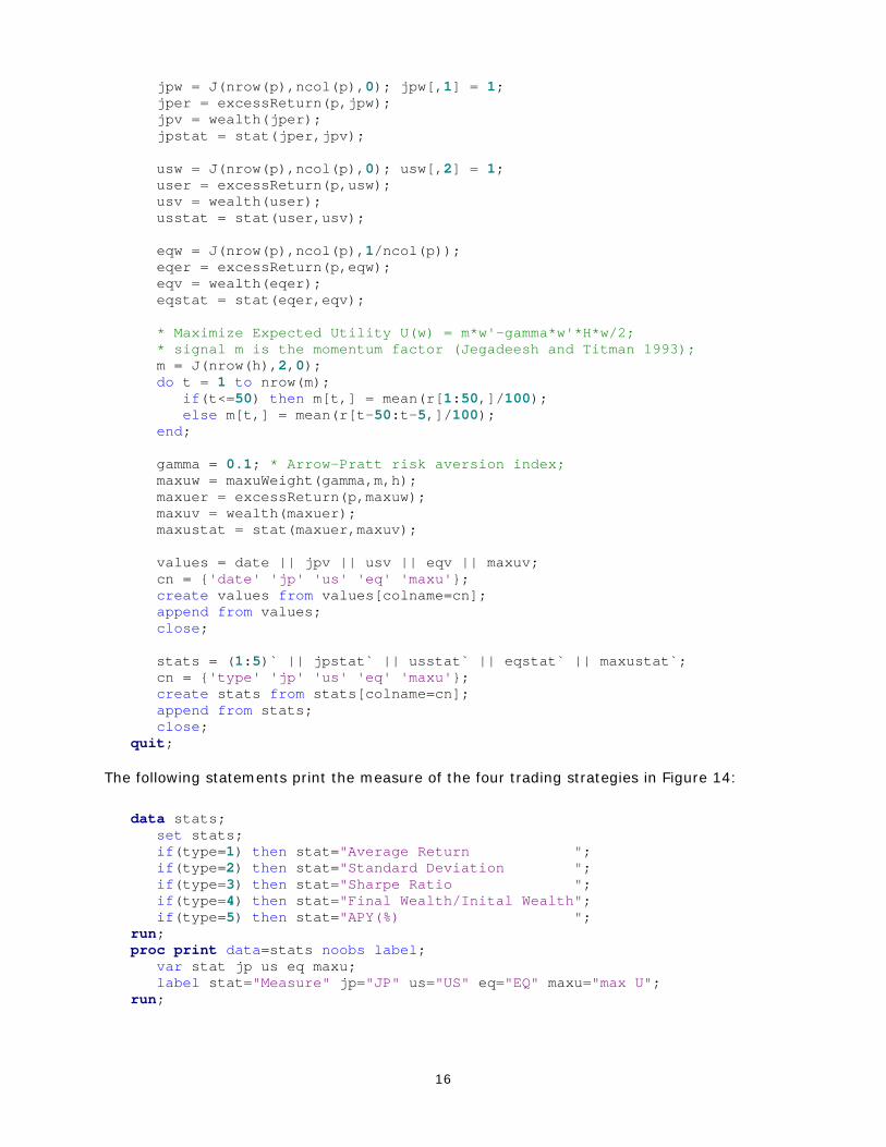
The following statements print the measure of the four trading strategies in Figure 14:

data stats;

set stats;

if(type=1) then stat="Average Return ";

if(type=2) then stat="Standard Deviation ";

if(type=3) then stat="Sharpe Ratio ";

if(type=4) then stat="Final Wealth/Inital Wealth";

if(type=5) then stat="APY(%) ";

run;

proc print data=stats noobs label;

var stat jp us eq maxu;

label stat="Measure" jp="JP" us="US" eq="EQ" maxu="max U";

run;

17

Figure 14. Measure of Four Trading Strategies

As shown in Figure 14, the max U strategy has both the best average return and the best

Sharpe ratio (an indicator of risk-adjusted return). Over 55 years, the final wealth that

results from using the max U strategy is about 60% more than the final wealth that results

from using the second-best strategy (US).

The following statements plot the wealth curve (or portfolio value) of each trading strategy

against time in Figure 15:

data values; set values; format date mmddyy10.; run;

proc sgplot data=values;

styleattrs datacontrastcolors=(black blue red green);

series x=date y=jp / legendlabel="JP";

series x=date y=us / legendlabel="US";

series x=date y=eq / legendlabel="EQ";

series x=date y=maxu / legendlabel="max U";

yaxis label="Wealth"; xaxis label="Date";

run;

18

Figure 15. Wealth Curves of the Four Trading Strategies

CONCLUSION

In this paper, three simple examples illustrate how easy it is to use the VARMAX procedure

to specify and estimate VAR, VECM, and multivariate GARCH models, and then how to infer

results and use them. For other multiple time series tools such as state space models

(SSMs) and hidden Markov models (HMMs), see the chapters “The SSM Procedure” in

SAS/ETS® 15.1: User’s Guide and “The HMM Procedure” in SAS® Econometrics 8.5:

Econometrics Procedures.

REFERENCES

Chen, Xilong, and Stefanos Kechagias. 2017. “Multivariate Time Series: Recent Additions to

the VARMAX Procedure.” Proceeding of the SAS Global Forum 2017 Conference. Cary, NC:

SAS Institute Inc. Available at https://support.sas.com/resources/papers/proceedings17/.

Jegadeesh, N., and S. Titman. 1993. “Returns to Buying Winners and Selling Losers:

Implications for Stock Market Efficiency.” The Journal of Finance 48(1):65–91.

Nobel Media AB. 2020a. “The Sveriges Riksbank Prize in Economic Science in Memory of

Alfred Nobel 2003.” NobelPrize.org. Accessed January 30, 2020.

https://www.nobelprize.org/prizes/economic-sciences/2003/summary/.

Nobel Media AB. 2020b. “The Sveriges Riksbank Prize in Economic Science in Memory of

Alfred Nobel 2011.” NobelPrize.org. Accessed January 30, 2020.

https://www.nobelprize.org/prizes/economic-sciences/2011/summary/.

Sims, C. A. 1980. “Macroeconomics and Reality.” Econometrica 48(1):1–48.

Stock, J. H., and M. W. Watson. 2001. “Vector Autoregressions.” Journal of Economic

Perspectives 15(4):101–115.

https://support.sas.com/resources/papers/proceedings17/

https://www.nobelprize.org/prizes/economic-sciences/2003/summary/

https://www.nobelprize.org/prizes/economic-sciences/2011/summary/

19

ACKNOWLEDGMENTS

The author would like to thank Jan Chvosta, Charles Sun, and Ji Shen for their valuable

comments and suggestions and Anne Baxter for her editorial review.

RECOMMENDED READING

• SAS/ETS 15.1: User’s Guide

• SAS Econometrics 8.5: Econometrics Procedures

• SAS Econometrics 8.5: Programming Guide

CONTACT INFORMATION

Your comments and questions are valued and encouraged. Contact the author at:

Xilong Chen

SAS Institute Inc.

[email protected]

SAS and all other SAS Institute Inc. product or service names are registered trademarks or

trademarks of SAS Institute Inc. in the USA and other countries. ® indicates USA

registration.

Other brand and product names are trademarks of their respective companies.

mailto:[email protected]

An Introduction to Multiple Time Series Analysis and the VARMAX … · 2000-01-01 · An...

Documents

Transcript of An Introduction to Multiple Time Series Analysis and the VARMAX … · 2000-01-01 · An...