An Introduction to Mechanism Design

Felix Munoz-Garcia

School of Economic Sciences

Washington State University1

1 Introduction

In this chapter, we consider situations in which some central authority wishes to implement a

decision that depends on the private information of a set of players. Here are two standard examples:

� A government agency may wish to choose the design of a public-works project (e.g., a bridge)based on preferences of its citizens. These preferences are, however, unobserved by the gov-

ernment as they are each citizen�s own private information.

� A monopolistic �rm may wish to identify the consumers�willingness to pay for the product

it produces with the goal of maximizing its pro�ts.

� A seller (auctioneer) selling an object (e.g., a painting) to a group of individuals, without

being able to observe their willingness to pay for the object.

Mechanism design is the study of what kinds of mechanisms the central authority (or themonopolist, or the seller, in the above examples) can devise in order to induce players (e.g., citi-

zens or consumers in the above examples) to reveal their private information (e.g., preferences for a

bridge, or willingness to pay for a product). For compactness, the central authority is often referred

to as the "mechanism designer".

2 Model: Mechanisms as Bayesian Games

Players: Each player i = f1; 2; :::; ng privately observes his type �i 2 �i which determines hispreferences over the public project (or his willingness to pay over the object for sale in an auction).

The pro�le of types for all n players, � = (�1; �2; : : : ; �n) ; is often referred to as the "state of

the world". State � is drawn randomly from the state space � � �1 � �2 � � � � � �n. The

draw of � is according to some prior distribution � (�) over �. While the speci�c draw �i is

player i�s private information, the distribution � (�) is common knowledge among all players. Manyapplications assume that every player i has quasilinear preferences, which eliminates wealth e¤ects.

In particular, a common utility function considers that player i�s utility is

vi (x; t; �i) = ui (x; �i) + ti

1 I appreciate the suggestions and comments of several students, specially Pak Choi.

1

where ui (x; �i) indicates player i�s utility from consuming x units of the good (e.g., public project

or good being sold at an auction) given his individual preference for such good, as captured by

parameter �i. Function ui(�) could be increasing (decreasing) in x 2 X when x represents a good

(bad, respectively), and made concave or convex in x depending on the application we seek to

study.2 Transfer ti is the amount of money given to (or taken away from) individual i: Such a

transfer can thus be positive, but can also be negative if money is taken away from individual i

(e.g., he pays ti to the central authority in order to fund the public project). An outcome would

be represented as y = (x; t1; � � � ; tN ), which describes, for instance, the amount of public projectto be provided, x, and the pro�le of transfers to each individual (which allows for some of them to

be positive, i.e., subsidies, while other can be negative, i.e., taxes).

Mechanism Designer: The mechanism designer has the objective of achieving an outcome

that depends on the types of players. For instance, the seller in an auction seeks to maximize

his revenue without being able to observe the valuations that each bidder has for the good; or a

government o¢ cial considering the construction of a bridge would like to maximize a social welfare

function without observing the preferences of his constituents for that bridge. Hence, most of our

subsequent discussion deals with the incentives that mechanism designers can provide to privately

informed agents (e.g., bidders or citizens in the above two examples) in order for them to voluntarily

reveal their private information.

We assume that the mechanism designer does not have a source of funds to pay the players.

That is, the monetary payments have to be self-�nanced, which implies thatPni=1 ti � 0. Hence,

whenPni=1 ti < 0; the mechanism designer keeps some of the money that he raises from players;

while if, instead,nPi=1ti = 0; all negative transfers collected from some players end up distributed to

other players, that is, the budget is balanced. Since, as de�ned above, an outcome is represented

as a vector y = (x; t1; � � � ; tN ), the set of outcomes is

Y =

((x; t1; � � � ; tN ) : x 2 X; ti 2 R for all i 2 N;

nXi=1

ti � 0)

In words, an outcome is an alternative x 2 X and a transfer pro�le (t1; t2:::; tn) such thatPni=1 ti � 0

holds. Finally, the mechanism designer�s objective is given by a choice rule

f (�) = (x (�) ; t1 (�) ; � � � ; tN (�)) ;

That is, for every pro�le of players�preferences � 2 �; the choice rule f(�) selects an alternativex(�) 2 X and a transfer pro�le (t1(�); t2(�); :::; tn(�)) satisfying

Pni=1 ti � 0:

2 In auction settings, x 2 X represents the assignment of the object for sale, thus becoming a vector x =(0; :::; 0; 1; 0; :::; 0) where 0 indicates that individual 1; ::; i � 1 did not receive the object for sale, as so did indi-viduals i+1; :::; N ; while a 1 indicates that individual i received the object. For this reason, in auctions x is referredto as an assignment or allocation of the object.

2

2.1 The Mechanism Game

Indirect revelation mechanism. An indirect revelation mechanism (IRM)

� = fS1; S2; : : : ; Sn; g (�)g

is a collection of n action sets S1; S2; : : : ; Sn and an outcome function g : S1 � S2 � � � � � Sn ! Y

that maps the actions chosen by the players into an outcome of the game: In this context, a pure

strategy for player i in the mechanism � is a function that maps his type �i 2 �i into an actionsi 2 Si, that is, si : �i ! Si: The payo¤s of the players are then given by vi (g (s) ; �i) ; which

depends on the outcome that emerges from the game g(s) when the action pro�le is s; and on

player i0s type �i (e.g., his preferences for a public project).

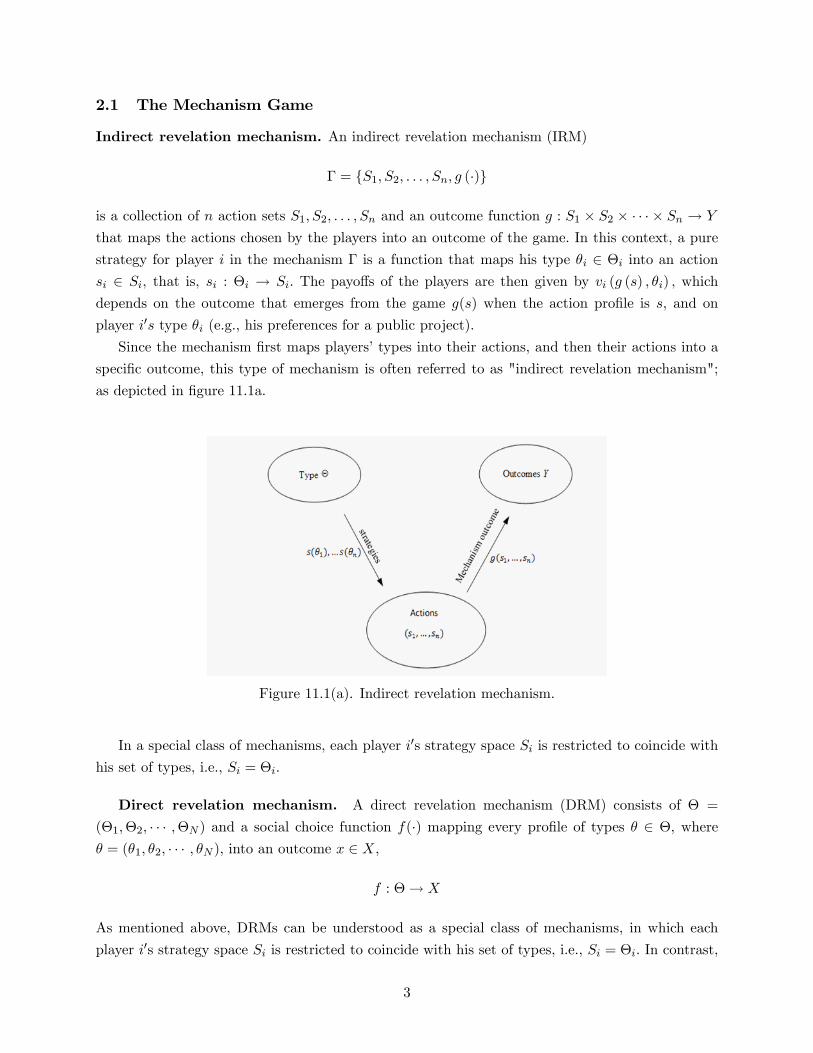
Since the mechanism �rst maps players�types into their actions, and then their actions into a

speci�c outcome, this type of mechanism is often referred to as "indirect revelation mechanism";

as depicted in �gure 11.1a.

Figure 11.1(a). Indirect revelation mechanism.

In a special class of mechanisms, each player i0s strategy space Si is restricted to coincide with

his set of types, i.e., Si = �i.

Direct revelation mechanism. A direct revelation mechanism (DRM) consists of � =

(�1;�2; � � � ;�N ) and a social choice function f(�) mapping every pro�le of types � 2 �, where� = (�1; �2; � � � ; �N ), into an outcome x 2 X,

f : �! X

As mentioned above, DRMs can be understood as a special class of mechanisms, in which each

player i0s strategy space Si is restricted to coincide with his set of types, i.e., Si = �i: In contrast,

3

IRMs require that, �rst, every player i chooses a strategy si 2 Si; such as a bid or a productionlevel, and then all players�strategies are mapped into an outcome. Figure 11.1b below depicts a

DRM, which could be understood as directly connecting the two unconnected balloons in the upper

part of �gure 11.1(a) rather than doing the "de-tour" of �rst mapping strategies into actions, and

then actions into outcomes.

Figure 11.1(b). Direct revelation mechanism

2.2 Examples of DRMs

The following examples explore a setting where a seller (agent 0) seeks to sell an indivisible object

to one of the two buyers (agents 1 and 2) so that the set of players is N = f0; 1; 2g. The set offeasible outcomes is

X = f(y0; y1; y2; t0; t1; t2) : yi 2 f0; 1g where2Xi=0

yi = 1 and ti 2 R 8i 2 Ng;

In words, the object is assigned to either the seller, y0 = 1, buyer 1, y1 = 1, or buyer 2, y2 = 1;

and a transfer ti is proposed to player i, if ti > 0, or a tax is imposed on him, if ti < 0. (At this

point, we do not require the mechanism to be budget balanced, which would imply that positive

and negative transfers o¤set each other at the aggregate level,P3i=1 ti = 0. We return to the budget

balance property in further sections.)

For an outcome x in the above set of feasible outcomes, i.e., x 2 X, every buyer�s utility is

ui(xi; �i) = �iyi + ti for all i = f1; 2g

where �i represents the buyer�s valuation for the object (which buyer i only enjoys if the object is

assigned to him, i.e., yi = 1); and ti is the positive (or negative) transfer he receives (or pays).

Example 1.1 - Direct revelation mechanism:Consider a setting in which the seller asks buyers 1 and 2 to simultaneously and independently

reveal their types (their valuation for the object), �1 and �2, and the seller assigns the object to

the agent with the highest revealed valuation �i. Without loss of generality, we assum that if there

is a tie, the object is assigned to buyer 1. More formally, for every pro�le of announced types,

4

� = (�1; �2), the assignment rule of this direct revelation mechanism is

y0(�) = 0

and

yi(�) =

(1 if �i � �j0 otherwise

where i = f1; 2g

and the transfer (or payment) rule is

ti(�) = ��i � yi(�) where i = f1; 2g

and

t0(�) = �[t1(�) + t2(�)] = �1 � y1(�) + �2 � y2(�)

In words, if player player i reports a larger valuation than his rival, �i � �j , he is assigned theobject, yi(�) = 1, paying a transfer equal to his reported valuation �i, i.e., ti(�) = ��i � 1 = ��i. Incontrast, his rival j does not receive the object, yj(�) = 0, thus entailing a zero transfer tj(�) = 0.

Finally, the seller receives the sum of the transfers, which in this setting is equivalent to the transfer

paid by the individual i who receives the object, that is, t0(�) = ti(�).

Example 1.2 - Direct revelation mechanism (variation of Example 1.1)Buyer 1 and 2 report �1 and �2 to the seller, the seller assigns the object to the buyer with the

highest announced report �i (that is, we use the same allocation rule yi(�) for i = f0; 1; 2g as inthe previous example), but the payment rule di¤ers:

ti(�) = ��j � yi(�)

and

t0(�) = �[t1(�) + t2(�)]

Intuitively, if player i reports a larger valuation than his rival, �i � �j , he is assigned the ob-ject, yi(�) = 1, but pays the second highest reported valuation, �j . A similar argument extends

to settings with N players, where ti(�) = �maxj 6=if�jg � yi(�), i.e., player i, if he is assigned theobject, pays a price equal to the highest competing reported valuation.

Example 1.3 - Procurement contractConsider a seller (0) and buyers 1 and 2, with the set of outcomes X being the same as that in

all previous examples, and the same utility function. However, the assignment rule is now reversed,

as the seller seeks to assign the service (e.g., public water management) to the �rm reporting the

lowest cost. That is, the assignment rule speci�es

y0(�) = 0

5

implying that the seller never keeps the object, and

yi(�) =

(1 if �i � �j0 otherwise

for every i = f1; 2g

That is, the procurement contract is assigned to the �rm announcing the lowest cost, �i � �j :Finally, the transfer rule coincides with that in Example 1.1 (if the winning agent is paid his costs)

or with that in Example 1.2 (if the winning agent is paid the cost of the losing �rm).

Example 2.1 - Funding a public projectA set of individuals N = f1; 2; � � � ; ng seek to build a bridge. Let k = 1 indicate that the bridge

is built, and k = 0 that it is not. The cost of the project is C > 0. Let ti be a transfer to agent

i, so �ti is a tax paid by agent i. The project is then built, k = 1, if total tax collection exceedsthe bridge�s total cost C � �

Pni=1 ti, but it is not build otherwise. (Alternatively, kC � �

Pni=1 ti

captures both the case in which the bridge is built and the case it is not.)

The set of outcomes, X, in this setting is then

X =

((k; t1; t2; � � � ; tn) : k 2 f0; 1g; ti 2 R; and kC � �

nXi=1

ti where i 2 N)

where, as usual in other sets of outcomes, speci�es the assignment rule k followed by transfer rule

to each agent i 2 N (which are allowed to be taxes since ti 2 R is not restricted to be positive).Utility function for every agent i is

ui(k; ti; �i) = k�i + ti

where �i can be interpreted as agent i�s valuation of the project. Note that agent i only enjoys

such a valuation if the bridge is built, k = 1, and that we allow for agent i to pay taxes if ti < 0.

Example 2.1.1 - Direct revelation mechanism in the public projectIn this case, the mechanism asks agents to directly report their types (i.e., their private valuation

for the bridge). In other words, the game restricts every player i�s strategy set to coincide with his

set of types, Si = �i. In this setting, the social choice function maps the reported (announced)

pro�le of types � � (�1; �2; � � � ; �n) into an assignment rule and a transfer rule. In particular, theassignment rule speci�es

k(�) =

(1 if

Pni=1 �i � C

0 otherwise

i.e., the project is built if and only if the aggregate reported valuation of all agents exceeds the

6

project�s cost. In addition, the transfer rule of this mechanism is

ti(�) = �C

nk(�)

i.e., if the project is built, k(�) = 1, then every agent i bears an equal share of its cost, Cn ; but if

the project is not built k(�) = 0; no agent has to pay anything, i.e., ti(�) = 0 for all agents i:

3 Implementation

3.1 Testing the implementability of SCF in direct revelation mechanism

Let us test the implementability of the scf described in Example 1.1 above. Suppose �1, �2 � U [0; 1]and i.i.d. In order to test if truthfully reporting his type �1 = �1; is a weakly dominant strategy

for player 1, let�s assume that player 2 truthfully reports his type, so his equilibrium strategy is

�2 � s�2(�2) = �2 and check for pro�table deviations for player 1. (Recall that this is the standardapproach to test whether a strategy pro�le is an equilibrium, where we �x the strategies of all N�1players and check if the remaining player has incentives to deviate from the proposed equilibrium

strategy.)

In particular, player 1 solves

max�1

(�1 � p) � probfwing = (�1 � �1) � probf�2 � �1g

where �1��1 represents the margin that player 1 keeps by under-reporting his valuation of the object(which helps him obtain the good at a lower price), while probf�2 � �1g denotes the probabilitythat player 1 wins the object because he reveals a larger valuation than player 2 to the seller.

Since �2 � U [0; 1], then probf�2 � �1g = F (�) = �1, which reduces player 1�s problem to

max�1

(�1 � �1) � �1 = �1�1 � �2

1

Taking FOCs with respect to �1 yields �1 � 2�1 = 0. Solving for �, we obtain an optimal

announcement of

�1 =�12

(An analogous argument applies to player 2: if player 1 truthfully reports his type, �1 = �1, then

player 2�s optimal report is �2 = �22 .) Hence, the SCF in Example 1.1 is not implementable as a

DRM since it doesn�t induce every player to truthfully report his type to the seller.

7

3.2 Incentive Compatibility

Therefore, player 1 shades his valuation in half, not truthfully reporting his type to the seller, so

�1 � s�1(�1) 6= �1. As suggested by Example 1.1, players may not have incentives to truthfully re-port their types in DRMs. This is, however, a desirable property that the mechanism designer will

try to guarantee in order to extract information from the agents. When a SCF induces privately

informed players to truthfully report their types in equilibrium, we refer to such SCF as �Incen-

tive Compatible�. We can, nonetheless, consider two types of incentive compatibilities depending

on whether truthtelling is an equilibrium in dominant strategies, or a Bayesian Nash Equilibrium

(BNE) of the incomplete information game.

Bayesian Incentive Compatibility, BIC: A SCF f(�) is BIC if the DRMD = ((�i)i2N ; f(�))has a BNE (s�1(�1); � � � ; s�n(�n)) in which s�i (�i) = �i for all �i 2 �i and all i 2 N .

That is, every player i �nds truthtelling optimal, given his beliefs about his opponents�types,

and given that all his opponents�strategies are �xed at truthtelling, s��i(��i) = ��i. More formally,

BIC entails that for every player i 2 N and every type �i 2 �i, and ��i 2 ��i,

E��i [ui(f(�i; ��i); �i)j�i] � E��i�ui(f(�

0i; ��i); �i)j�i

�for every misreport �0i 6= �i. This inequality just says that player i; prefers to truthfully report histype �i; yielding an outcome f(�i; ��i) than misreporting his type to be �0i 6= �i; which would yieldan outcome f(�0i; ��i): Importantly, player i prefers to truthfully reveal his type �i in expectation,

as he doesn�t observe the pro�le of types of his rivals ��i 2 ��i: As a consequence, the abovede�nition could allow player i to �nd truthtelling optimal for some values of his rivals�types ��i;

but not for others as long as in expectation he prefers to truthfully report his type �i: The following

version of incentive compatibility is more demanding , as it requires player i to �nd truthtelling

optimal regardless of the speci�c realization of this rivals�types ��i; and regardless of his rivals�

announcements. That is, we next focus on SCFs for which truthtelling becomes a dominant strategy

for every player i 2 N:

Dominant Strategy Incentive Compatibility, DSIC: A SCF f(�) is DSIC if the DRM

D = ((�i)i2N ; f(�)) has a dominant strategy equilibrium (s�1(�1); � � � ; s�n(�n)) in which s�i (�i) = �ifor all �i 2 �i and all i 2 N .

Therefore, every player i �nds truthtelling optimal regardless of his beliefs about his opponents�

types, and independently on his opponents�strategies in equilibrium, i.e., both when they truthfully

report their types, s��i(��i) = ��i, and when they do not, s��i(��i) 6= ��i. More formally, DSIC

entails that for every player i 2 N and every type he may have �i 2 �i,

ui(f(�i; s�i); �i) � ui(f(�0i; s�i); �i)

8

where s�i 2 S�i, for all �0i 6= �i. Then, DSIC is a more demanding property than BIC, in partic-ular, DSIC requires that players �nd truthtelling optimal regardless of the speci�c types of their

opponents and independently on their speci�c actions in equilibrium. In contrast, BIC asks for

truthtelling to be utility maximizing only in expectation and given that all other players are truth-

fully reporting their types. In addition, note that DSIC requires that player i �nds it optimal

to truthfully reveal his type �i both when his rivals choose equilibrium strategies, i.e., when they

truthfully report their types and thus s�i = ��i, but also when they don�t, i.e., when they misreport

their types, s�i 6= ��i.Finally, DSIC is often referred to as "strategy-proof" or "truthful", since players cannot �nd an

alternative strategy (misreporting their types) that would yield a larger payo¤.

4 Indirect Revelation Mechanism

An indirect revelation mechanism (IRM) allows strategy spaces to di¤er from a direct announce-

ment of types, i.e., Si 6= �i, or to coincide, Si = �i, for every player i 2 N . In that regard, a

DRM can then be interpreted as a special case of IRM whereby players�strategies are restricted

to coincide with their type space, i.e., when Si = �i we only allow players to report a type

(either truthfully or misreporting) but they cannot do anything else. In contrast, in an IRM

players can potentially choose from a richer strategy space. Once every player chooses his strat-

egy Si, and a pro�le of strategies emerges s = (s1; s2; :::; sn), the IRM maps such strategy pro�le

s � (s1; s2; � � � ; sn) into an outcome g(s). The equilibrium that arises in the IRM has every player i;

choosing a strategy as a function of privately observed type, s�i (�i); yielding an equilibrium strategy

pro�le s�(�) = (s�1(�1); � � � ; s�n(�n)) : Such strategy pro�le entails an equilibrium outcome g(s�(�)):

A natural question is whether the equilibrium oucome g(s�(�)) emerging from the IRM, whereby

everyplayer freely choose an action which ultimately gives rise to an outcome of the game. For

completeness, we explore this coincidence in outcomes (which is referred to as that the IRM im-

plements the planner�s SCF) �rst using dominant strategies and then using BNE (as for incentive

compatibility).

4.1 Implementation in Dominant Strategies

A mechanism M = ((Si)i2N ; g(�)) implements the SCF f(�) in dominant strategy equilibrium if

there is a weakly dominant strategy pro�le s�(�) = (s�i (�1); � � � ; s�n(�n)) of the Bayesian gameinduced by the mechanism M such that

g (s�(�)) = f(�) for all � 2 �

Example: Second-price auctions implement the SCF in Example 1.2 in weakly dominant strat-

9

egy equilibrium. In particular, the strategy set for every bidder i is his set of feasible bids, which

in the case of positive bids without the existence of a reservation prize simpli�es to Si = R+. Inthis context, we showed that every bidder i �nds that a bid of si(�i) = �i (bids coinciding with

his valuation) constitutes a weakly dominated strategy in the second-price auction, i.e., he would

choose it regardless of his opponents�valuations for the object and independently of their bidding

pro�le s�i. Hence, the object is assigned to the bidder submitting the highest bid, who pays a

price equal to the second highest bid. This outcome that coincides with the SCF in Example 1.2

whereby the social planner could observe all bidders�valuations, �.

4.2 Implementation in BNE

A mechanism M = ((Si)i2N ; g(�)) implements the SCF f(�) in BNEs if there is a BNE strategypro�le s�(�) = (s�i (�1); � � � ; s�n(�n)) of the Bayesian game induced by the mechanism M such that

g (s�(�)) = f(�) for all � 2 �

Example: Recall that the SCF of Example 1.3 is BIC, since for every �, the equilibrium strategy

satis�es truthtelling, i.e., s�i (�i) = �i for all i 2 N . In addition, we can use FPA as an IRM that

implements SCF of Example 1.3 in its BNE.

The above discussion suggests a connection between the outcomes of a DRM that induces

truthtelling and an IRM. In particular, we might wonder if, for a given SCF mapping pro�les of

types into socially desirable outcomes, we can design a clever game (a IRM) in which equilibrium

play would yield the exact same outcome as that identi�ed by the SCF. The answer is positive

(although we discuss some disadvantages later), and it is known in the literature as the �Revelation

Principle�. The next sections separately present it for the cases of BNE and dominant strategies.

Figure 11.2 depicts the revelation principle by combining left and right panels of �gure 11.1. In

the upper part of the �gure illustrates a direct revelation mechanism mapping types into outcomes

through a social choice function. The lower part, in contrast, takes an "indirect route" by �rst

allowing every player to map his own type into a strategy, i.e., si(�i) for every i 2 N; and thentaking the action pro�le and mapping into an outcome of the game. The question that the revelation

principle asks is then whether we can �nd game rules that provide players with the incentives to

choose strategies that ultimately lead to outcomes coinciding with those selected by a social choice

10

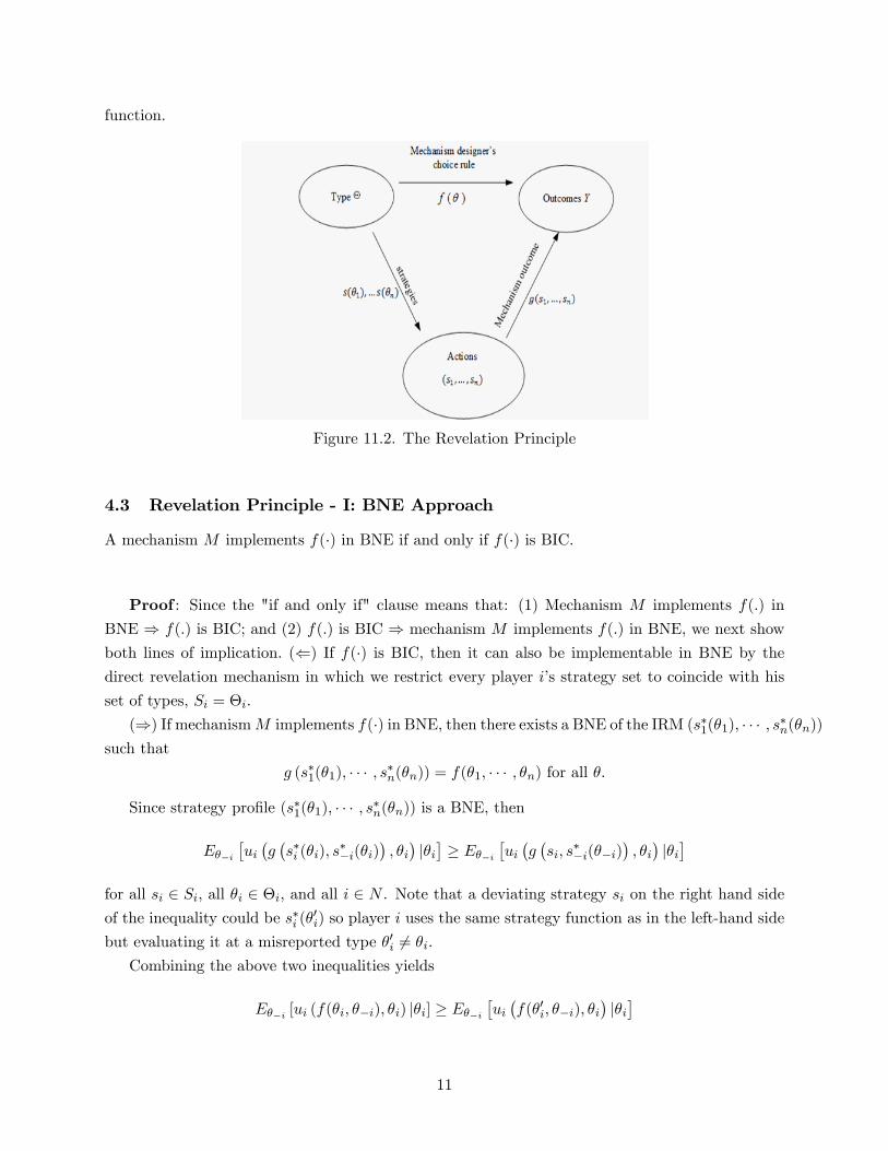
function.

Figure 11.2. The Revelation Principle

4.3 Revelation Principle - I: BNE Approach

A mechanism M implements f(�) in BNE if and only if f(�) is BIC.

Proof : Since the "if and only if" clause means that: (1) Mechanism M implements f(:) in

BNE ) f(:) is BIC; and (2) f(:) is BIC ) mechanism M implements f(:) in BNE, we next show

both lines of implication. (() If f(�) is BIC, then it can also be implementable in BNE by thedirect revelation mechanism in which we restrict every player i�s strategy set to coincide with his

set of types, Si = �i.

()) If mechanismM implements f(�) in BNE, then there exists a BNE of the IRM (s�1(�1); � � � ; s�n(�n))such that

g (s�1(�1); � � � ; s�n(�n)) = f(�1; � � � ; �n) for all �:

Since strategy pro�le (s�1(�1); � � � ; s�n(�n)) is a BNE, then

E��i�ui�g�s�i (�i); s

��i(�i)

�; �i�j�i�� E��i

�ui�g�si; s

��i(��i)

�; �i�j�i�

for all si 2 Si, all �i 2 �i, and all i 2 N . Note that a deviating strategy si on the right hand sideof the inequality could be s�i (�

0i) so player i uses the same strategy function as in the left-hand side

but evaluating it at a misreported type �0i 6= �i.Combining the above two inequalities yields

E��i [ui (f(�i; ��i); �i) j�i] � E��i�ui�f(�0i; ��i); �i

�j�i�

11

for all �0i 6= �i, all �i 2 �i, and all i 2 N , which is exactly the condition that we need for SCF f(�)to be BIC. (Q.E.D.)

4.4 Revelation Principle - II: DSIC Approach

A mechanism M implements f(�) in dominant strategy equilibrium if and only if f(�) is DSIC.

Proof : In this case we also need to show both directions of the "if and only if" clause. (()Identical as the �rst step of the above proof.

()) Similar to the previous proof, but we do not need that every player i takes expectationsof his opponents� types, and we don�t need him to �x his opponents� strategies in equilibrium,

s��i(��i), but instead he considers any strategy of his opponents, s�i(��i).

As a practice, let us develop the proof. If M implements f(�) in dominant strategy equilibrium(DSE), there exists a weakly dominant BNE, (s�1(�1); � � � ; s�n(�n)) such that

g (s�1(�1); � � � ; s�n(�n)) = f(�1; � � � ; �n) for all �:

Since strategy pro�le (s�1(�1); � � � ; s�n(�n)) is a dominant strategy equilibrium of the mechanism

M ,

ui (g (s�1(�1); s�i(��i))) � ui (g (si; s�i(��i)) ; �i)

for all si 2 Si, all �i 2 �i, all ��i 2 ��i, all s�i 2 S�i, and all i 2 N . In words, player i does nothave incentives to deviate, i.e., of choosing a strategy si = s�i (�i); for any type �i he may have, any

pro�le of types his opponents may have, ��i; and for any strategy pro�le they may choose s�i(��i):

Similarly as in the above proof, the deviating strategy si on the right-hand side of the inequality

could be s�i (�0i) whereby player i uses the same function as in the left-hand side but evaluated at a

misreported type �0i 6= �i.Combining the above conditions yields

ui (f(�i; ��i); �i) � ui�f(�0i; ��i); �i

�which exactly coincides with the condition that we need for the SCF to be DSIC. (Q.E.D.)

In summary, the revelation principle in its two versions tells use that

A mechanism M implements f(�) in BNE() f(�) is BIC

A mechanism M implements f(�) in DSE() f(�) is DSIC

Hence, if a mechanism is not BIC or DSIC, (i.e., telling the truth is not an equilibrium in the

12

DRM), then we cannot �nd a clever game or institutional setting (an IRM) that implements such

a SCF f(�). Alternatively, if a mechanism M is BIC, we can �nd an IRM that implements f(�) inBNE. Similarly, if a mechanism is DSIC, we can �nd an IRM that implements f(�) in DSE.

5 VCG mechanism

In most of the sections hereafter we consider the following quasilinear preferences

vi(k; �i) = ui(k; �i) + wi + ti

where k 2 K describes, as usual, the assignment rule (e.g. k = f0; 1g representing if a publicproject is implemented, k = 1; or not k = 0). In standard settings, �i 2 �i, wealth is strictlypositive, wi > 0, and ti > 0 denotes that player i receives a net transfer while ti < 0 indicates that

he pays to the system. In addition,Pi2N ti � 0 indicates budget balance. In particular, if such

condition holds with equality, we refer to it as �strong budget balance�, while otherwise we refer

to it as �weak budget balance�since it allows for the system to run a de�cit (or a surplus) at the

aggregate level.

5.1 Allocative e¢ ciency

We say that a SCF f(�) = (k(�); t1(�); � � � ; tn(�)) satis�es allocative e¢ ciency if, for every pro�leof types � 2 �, the allocation function k(�) satis�es

k(�) 2 argmaxk2K

Xi2N

ui(k; �i)

That is, k(�) allocates objects (or public projects) in order to maximize aggregate payo¤s for

each pro�le of types, �.3 The following examples test whether the allocation function k(�) in two

di¤erent SCF satis�es allocative e¢ ciency (AE).

Example 2.1 - Public project with an allocative e¢ cient SCFConsider a setting with two agents N = f1; 2g each with two types �i = f20; 60g for all

i = f1; 2g. Their utility function is

ui(k; �i) = k(�i � 25)

which indicates that if the project is not implemented, k = 0, agents�utilities are zero; but if it

is implemented, k = 1, both agents bear an equal cost of 25. Consider the following allocation

3Hence, allocative e¢ ciency is analog to Pareto e¢ ciency. However, since most mechanism design problems dealwith the allocation of property rights (e.g., auctions and procurement contracts) and the implementation of publicprojects, we normally use the concept of allocative e¢ ciency.

13

function

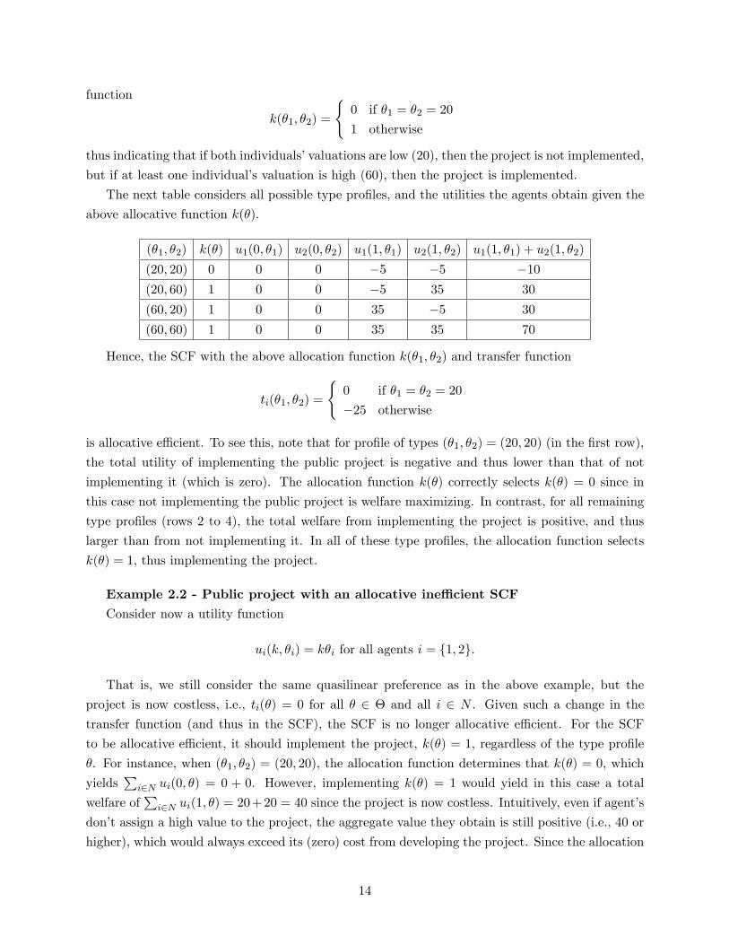
k(�1; �2) =

(0 if �1 = �2 = 20

1 otherwise

thus indicating that if both individuals�valuations are low (20), then the project is not implemented,

but if at least one individual�s valuation is high (60), then the project is implemented.

The next table considers all possible type pro�les, and the utilities the agents obtain given the

above allocative function k(�).

(�1; �2) k(�) u1(0; �1) u2(0; �2) u1(1; �1) u2(1; �2) u1(1; �1) + u2(1; �2)

(20; 20) 0 0 0 �5 �5 �10(20; 60) 1 0 0 �5 35 30

(60; 20) 1 0 0 35 �5 30

(60; 60) 1 0 0 35 35 70

Hence, the SCF with the above allocation function k(�1; �2) and transfer function

ti(�1; �2) =

(0 if �1 = �2 = 20

�25 otherwise

is allocative e¢ cient. To see this, note that for pro�le of types (�1; �2) = (20; 20) (in the �rst row),

the total utility of implementing the public project is negative and thus lower than that of not

implementing it (which is zero). The allocation function k(�) correctly selects k(�) = 0 since in

this case not implementing the public project is welfare maximizing. In contrast, for all remaining

type pro�les (rows 2 to 4), the total welfare from implementing the project is positive, and thus

larger than from not implementing it. In all of these type pro�les, the allocation function selects

k(�) = 1, thus implementing the project.

Example 2.2 - Public project with an allocative ine¢ cient SCFConsider now a utility function

ui(k; �i) = k�i for all agents i = f1; 2g:

That is, we still consider the same quasilinear preference as in the above example, but the

project is now costless, i.e., ti(�) = 0 for all � 2 � and all i 2 N . Given such a change in thetransfer function (and thus in the SCF), the SCF is no longer allocative e¢ cient. For the SCF

to be allocative e¢ cient, it should implement the project, k(�) = 1, regardless of the type pro�le

�. For instance, when (�1; �2) = (20; 20), the allocation function determines that k(�) = 0, which

yieldsPi2N ui(0; �) = 0 + 0. However, implementing k(�) = 1 would yield in this case a total

welfare ofPi2N ui(1; �) = 20+20 = 40 since the project is now costless. Intuitively, even if agent�s

don�t assign a high value to the project, the aggregate value they obtain is still positive (i.e., 40 or

higher), which would always exceed its (zero) cost from developing the project. Since the allocation

14

function k(�) described above does not implement the project when both individuals�valuations

are low, i.e., when (�1; �2) = (20; 20); we can conclude that allocation function k(�), and thus the

SCF, are not allocative e¢ cient.

5.2 Ex-post e¢ ciency and Quasilinear preferences

We say that a SCF f(�) is ex-post e¢ cient if, for every type pro�le � 2 �, the outcome chosen bythe SCF, f(�) = x; maximizes the sum of all agents�utilities. That is,X

i2Nui (f(�); �i) �

Xi2N

ui(x; �i); for all feasible outcomes x 2 X

We check that from an ex-post perspective: after observing all players�types in vector �. An

interesting property of ex-post e¢ ciency is that, under quasilinear preferences, it is equivalent to

saying that the SCF is allocative e¢ cient and budget balanced, as we show in Appendix 1.

6 Examples of common mechanisms

We next present some famous mechanisms extensively used in theoretical and applied literature. In

particular, we are interested in showing that the SCF they implement satis�es AE, i.e., we cannot

�nd alternative outcomes that could increase social surplus, and DSIC, i.e., agents �nd it optimal

to truthfully reveal their private information �i to the mechanism designer independently on what

their rivals do.

6.1 Groves Theorem

Let the SCF f(�) = (k(�); t1(�); � � � ; tn(�)) satisfy AE. Then f(�) satis�es DSIC if transfer functionscan be represented by

ti(�i; ��i) =Xj 6=i

uj (k(�); �j) + hi(��i)

where hi : �! R is an arbitrary function.

Intuitively, the transfer that player i receives depends on the utility that all other agents expe-

rience from the pro�le of announced types, i.e., the externality that player i�s announcement causes

on their well-being (as the allocation rule considers the entire pro�le of preferences �), plus a func-

tion hi(��i) which is independent on player i�s announcement. If player i changes his report from

15

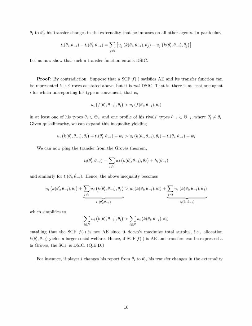
�i to �0i, his transfer changes in the externality that he imposes on all other agents. In particular,

ti(�i; ��i)� ti(�0i; ��i) =Xj 6=i

�uj (k(�i; ��i); �j)� uj

�k(�0i; ��i); �j

��Let us now show that such a transfer function entails DSIC.

Proof : By contradiction. Suppose that a SCF f(�) satis�es AE and its transfer function canbe represented à la Groves as stated above, but it is not DSIC. That is, there is at least one agent

i for which misreporting his type is convenient, that is,

ui�f(�0i; ��i); �i

�> ui (f(�i; ��i); �i)

in at least one of his types �i 2 �i, and one pro�le of his rivals�types ��i 2 ��i, where �0i 6= �i.Given quasilinearity, we can expand this inequality yielding

ui�k(�0i; ��i); �i

�+ ti(�

0i; ��i) + wi > ui (k(�i; ��i); �i) + ti(�i; ��i) + wi

We can now plug the transfer from the Groves theorem,

ti(�0i; ��i) =

Xj 6=i

uj�k(�0i; ��i); �j

�+ hi(��i)

and similarly for ti(�i; ��i). Hence, the above inequality becomes

ui�k(�0i; ��i); �i

�+Xj 6=i

uj�k(�0i; ��i); �j

�| {z }

ti(�0i;��i)

> ui (k(�i; ��i); �i) +Xj 6=i

uj (k(�i; ��i); �j)| {z }ti(�i;��i)

which simpli�es to Xi2N

ui�k(�0i; ��i); �i

�>Xi2N

ui (k(�i; ��i); �i)

entailing that the SCF f(�) is not AE since it doesn�t maximize total surplus, i.e., allocation

k(�0i; ��i) yields a larger social welfare. Hence, if SCF f(�) is AE and transfers can be expressed ala Groves, the SCF is DSIC. (Q.E.D.)

For instance, if player i changes his report from �i to �0i, his transfer changes in the externality

16

that he imposes on all other agents. In particular,24Xj 6=i

uj(k(�i; ��i); �j) + hi(��i)

35�24Xj 6=i

uj(k(�0i; ��i); �j) + hi(��i)

35=

Xj 6=i

uj(k(�i; ��i); �j)�Xj 6=i

uj(k(�0i; ��i); �j)

=Xj 6=i

�uj(k(�i; ��i); �j)� uj(k(�0i; ��i); �j)

�6.2 Clarke (Pivotal) mechanisms

This type of mechanisms constitute a special class of Groves mechanisms described above, in which

the function hi(��i) takes the form

hi(��i) = �Xj 6=i

uj (k�i(��i); �j) for all ��i 2 ��i; and for all i 2 N

where k�i(��i) denotes the allocation that the SCF selects when considering all agents j 6= i, i.e.,as if player i was absent.

Hence, the transfer becomes

ti(�) =Xj 6=i

uj (k(�); �j) + hi(��i)

=Xj 6=i

uj (k(�); �j)�Xj 6=i

uj (k�i(��i); �j)| {z }Clarke hi(��i) function

for all i 2 N

Intuitively, the �rst term represents the total value that all j 6= i agents obtain when the seller(mechanism designer) considers player i�s preferences when allocation k(�) is being determined.

The second term, in contrast, describes the total value that they obtain when the seller ignores

player i�s preferences, so the allocation becomes k(��i). Therefore, the di¤erence between both

terms captures the marginal contribution that player i�s preferences have on the mechanism�s allo-

cation. In this sense, the Clarke mechanism is pivotal, as every individual i plays a pivotal role in

determining the transfer that other players receive (or pay) by having player i participating in the

mechanism.

Example of VCG mechanism - IConsider 5 bidders participating in a second price auction (SPA), whose valuations

v1 = 20; v2 = 15; v3 = 12; v4 = 10; v5 = 6

Hence, submitting a bid equal to his valuation, bi(vi) = vi for all vi and all i 2 N; is a BNE of the

17

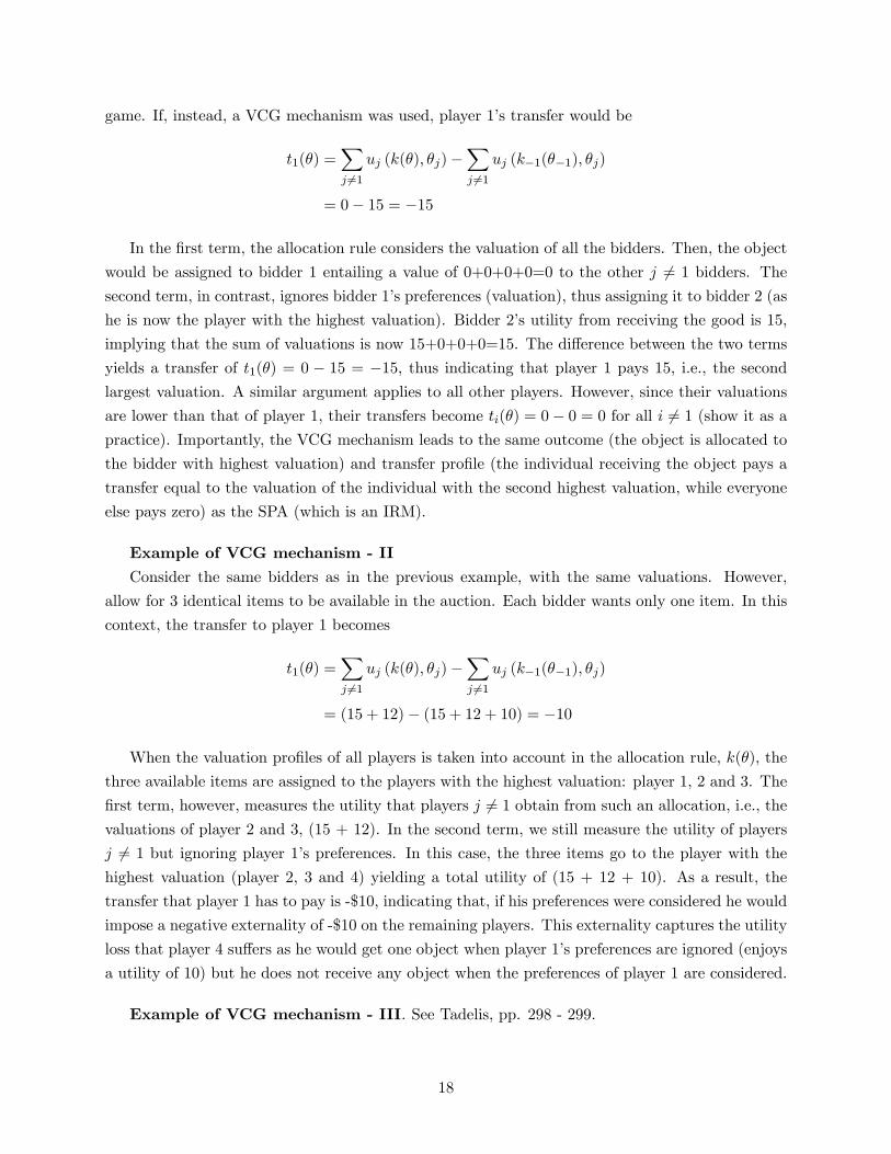
game. If, instead, a VCG mechanism was used, player 1�s transfer would be

t1(�) =Xj 6=1

uj (k(�); �j)�Xj 6=1

uj (k�1(��1); �j)

= 0� 15 = �15

In the �rst term, the allocation rule considers the valuation of all the bidders. Then, the object

would be assigned to bidder 1 entailing a value of 0+0+0+0=0 to the other j 6= 1 bidders. The

second term, in contrast, ignores bidder 1�s preferences (valuation), thus assigning it to bidder 2 (as

he is now the player with the highest valuation). Bidder 2�s utility from receiving the good is 15,

implying that the sum of valuations is now 15+0+0+0=15. The di¤erence between the two terms

yields a transfer of t1(�) = 0 � 15 = �15, thus indicating that player 1 pays 15, i.e., the secondlargest valuation. A similar argument applies to all other players. However, since their valuations

are lower than that of player 1, their transfers become ti(�) = 0� 0 = 0 for all i 6= 1 (show it as apractice). Importantly, the VCG mechanism leads to the same outcome (the object is allocated to

the bidder with highest valuation) and transfer pro�le (the individual receiving the object pays a

transfer equal to the valuation of the individual with the second highest valuation, while everyone

else pays zero) as the SPA (which is an IRM).

Example of VCG mechanism - IIConsider the same bidders as in the previous example, with the same valuations. However,

allow for 3 identical items to be available in the auction. Each bidder wants only one item. In this

context, the transfer to player 1 becomes

t1(�) =Xj 6=1

uj (k(�); �j)�Xj 6=1

uj (k�1(��1); �j)

= (15 + 12)� (15 + 12 + 10) = �10

When the valuation pro�les of all players is taken into account in the allocation rule, k(�); the

three available items are assigned to the players with the highest valuation: player 1, 2 and 3. The

�rst term, however, measures the utility that players j 6= 1 obtain from such an allocation, i.e., the

valuations of player 2 and 3, (15 + 12). In the second term, we still measure the utility of players

j 6= 1 but ignoring player 1�s preferences. In this case, the three items go to the player with the

highest valuation (player 2, 3 and 4) yielding a total utility of (15 + 12 + 10). As a result, the

transfer that player 1 has to pay is -$10, indicating that, if his preferences were considered he would

impose a negative externality of -$10 on the remaining players. This externality captures the utility

loss that player 4 su¤ers as he would get one object when player 1�s preferences are ignored (enjoys

a utility of 10) but he does not receive any object when the preferences of player 1 are considered.

Example of VCG mechanism - III. See Tadelis, pp. 298 - 299.

18

7 Groves mechanism and budget balance (technical)

Is the Groves mechanism budget balanced? Not necessarily. As the next result from Green and

La¤ont4 (1979) shows, if the set of possible types is su¢ ciently rich, no social choice function

satis�es DSIC and ex-post e¢ cient (which would require a k(�) function maximizing total surplus

and transfers being budget balanced,Pi2N ti (�) = 0.)

Green-La¤ont impossibility theorem. Suppose that for each agent i 2 N , that

F = fvi(�; �i) such that �i 2 �ig:

that is, every possible valuation function from k to R arises for some �i 2 �i: Then, there is noSCF that is DSIC and ex-post e¢ cient (EPE).

In other words, either agents have to overpay,Pi2N ti (�) < 0 for some �i, or have an ine¢ cient

project selection, i.e., a project for which we could �nd an alternative allocation k0 6= k (�) that

yields a larger total surplus.

Some good news: if the preferences of at least one agent are common knowledge (such as the

seller in an auction), then we can �nd SCFs that satisfy DSIC and EPE (and hence BB), as we

next show.

Budget balance of Groves mechanisms: If there is at least one agent whose preferencesare known (that is, his type set is a singleton) then it is possible to identify a function hi (�) in theGroves mechanism that yields BB, i.e.,

Pi2N ti (�) = 0.

Proof : Let agent 0�s preferences be known, �0 = f�0g. In this setting, EPE holds when wechoose transfer functions (t1 (�) ; :::; tN (�)) for the N agents whose preferences are unknown, as

long as they satisfy

t0 (�) = �Xi6=0

ti (�) for all �

That is, ifPi2N ti (�) < 0 then agent 0 receives the total transfers of all other N individuals,

and ifPi2N ti (�) > 0 agent 0 pays the de�cit in contributions by the N individuals. Intuitively,

agent 0 can be understood as the a government agency that absorbs surpluses or compensates for

de�cits. (Q.E.D.)

8 Participation constraints

Thus far we assumed that all agents participated in the mechanism, as if participation was com-

pulsory by some government agency. But what if their participation is voluntary? We then need

to add participation constraints (PC) to each agent with type �i.

4Green, J.R. and La¤ong, J. J. (1979). Incentives in Public Decision Making (Amsterdam: North-Holland).

19

We will next present di¤erent approaches to write the PC, depending on the information that

the agent knows when the PC constraint is de�ned:

� Before he knows his type (ex-ante stage);

� After knowing his type, but without observing his opponents type ��i (interim stage); and

� After knowing his type, and the announcements of all other individuals (ex-post stage)

Using ui (�i) to denote agent i�s reservation utility, the PC in the above three stages becomes

Ex-ante PC: E�[ui(g(�i; ��i); �i)] � E�i [ui(�i)]

Interim PC: E��i [ui(g(�i; ��i)j�i)] � ui(�i) for all �iEx-post PC: ui(g(�i; ��i); �i) � ui(�i) for all (�i; ��i)

At the ex-ante stage, individual i takes expectations of both his own type, �i; and his rivals�, ��i;

since he could not observe his own type yet. At the interim stage, he only takes the expectations

of his rivals�types, ��i; while at the ex-post stage he does not need to take expectations since all

the type pro�les � = (�i; ��i) have been revealed. As you can anticipate, for any SCF g (�)

Ex-post PC ) Interim PC ) Ex-ante PC

which occurs because the ex-post de�nition is more demanding (for all (�i; ��i) pairs) than the

interim de�nition (for all �i), and both are more demanding than the ex-ante de�nition. In the

following subsections we apply the above PC de�nitions to di¤erent settings, such as under a groves

mechanism, and under a Clarke mechanism, among others.

8.1 Participation constraints in the VCG mechanism

Example 1 - Public good projectConsider a society with two individuals N = f1; 2g. A public project is either implemented or

not, k = f0; 1g; and both individuals�private valuations for the project are drawn from �1 = �2 =

f20; 60g. Finally, the total cost of building the project is 50.In this setting, the set of feasible outcomes is

X = f(k; t1; t2) : k = f0; 1g; t1; t2 2 R; �(t1 + t2) � 50g

That is, allocation rules k = f0; 1g and transfer rules that guarantee total payments of $50.Consider the allocation function we considered in previous sections for this example (where the

20

project is implemented if at least the valuation of one individual is 60), which we reproduce below:

k� (�1; �2) =

(0 if �1 = �2 = 20

1 otherwise

and de�ne the same valuation function as in previous section

vi (k� (�1; �2) ; �i) = k

� (�1; �2)| {z }.&

1 0

� (�i � 25)| {z }margin

for all �1; �2

Recall from previous sections that such allocation rule is AE. From the Groves�theorem, we

know that if the transfer function is �à la Groves�then the resulting SCF satis�es DSIC. Let us now

check if, despite being DSIC, such SCF violates ex-post PC. In particular, assume that reservation

utility is ui (�i) = 0 for all �i and for all i 2 N . Hence, for ex-post PC, we need

ui (g (�i; ��i) ; �i) � 0 for all �1 2 �1; and all �2 2 �2

In the case that (�1; �2) = (20; 60), such condition requires

v1 (k� (20; 60) ; 20)| {z }

�5

+ t1 (20; 60) � 0

which reduces to �5 + t1 (20; 60) � 0, or t1 (20; 60) � 5. Now consider a di¤erent pro�le of types(�1; �2) = (60; 60). Since SCF is DSIC, we need truthtelling,

v1 (k� (60; 60) ; 60)| {z }

=35

+ t1 (60; 60)| {z }�5

� v1 (k� (20; 60) ; 20)| {z }

=35| {z }=)

+ t1 (20; 60)| {z }#�5

Intuitively, misreporting doesn�t a¤ect the probability of the public project being implemented,

nor player 1�s valuation for the public project. Hence, the project is infeasible since total transfers

fall short of the total cost,

t1 (20; 60) + t2 (60; 60) � 10 < 50 = total cost.

8.2 Participation constraints in Clarke mechanism

Clarke mechanisms satisfy ex-post PC if they satisfy the following properties:

1. Reservation utility is zero, ui (�i) = 0 for all �i 2 �i

2. The mechanism satis�es "choice set monotonicity": The set of feasible outcomes X weakly

grows in N . The intuition behind this assumption is that the choice set X becomes wider as

more agents enter the population.

21

3. The mechanism satis�es "no negative externality": Formally, the utility that player i obtains

a positive utility when his preferences �i are ignored, vi�k��i (��i) ; �i

�� 0 where allocation

k��i (��i) is AE for all �i 2 �i; all ��i 2 ��i; and all i 2 N . In words, player i obtains apositive value from the allocation that emerges when his preferences are ignored. Otherwise,

the preferences of all other agents would lead to an allocation k��i(��i) that imposes a negative

externality on player i.

Let us next show why the above three properties help guarantee that the Clarke Mechanism

satis�es ex-post PC.

Proof : Recall that, given the transfer function in the Clarke mechanism, the utility functionui (g(�); �) becomes

ui(g (�); �) = vi (k�(�); �) +

24Xj 6=i

vj (k�(�); �j)�

Xj 6=i

vj�k��i(��i); �j

�35| {z }

ti(�i;��i)

=Xj

vj (k�(�); �j)| {z }

the �rst two terms

in the above expression

�Xj 6=i

vj�k��i(��i); �j

�

From choice set monotonicity, the choice with agent i, k�(�), must generate the same or more

total value than the choice without him, k��i(��i). Hence, the above expression becomes (where we

only changed the �rst term in the right-hand side)

ui(g (�); �) �Xj

vj�k��i(��i); �j

��Xj 6=i

vj�k��i(��i); �j

�In addition, the right-hand side simpli�es to vi(k��i(��i); �i) since the �rst term in the right-hand

side of the above expression includes utility of agent i while the second term does not. Therefore,

the above expression reduces to

ui(g (�); �) � vi(k��i(��i); �i) � 0 = ui(�i)

where the �� 0" inequality originates from the "no negative externality" property. Hence, ui(g (�); �) �ui (�i) holds for all � 2 �, as required for the SCF to satisfy ex-post PC. (Q.E.D.)

Examples of ex-post mechanisms are the �rst price auction, and the second price auction (which,

as shown above, is a special case of Clarke mechanism). Check the ex-post e¢ ciency of these two

auction formats as a practice.

22

8.3 dAGVA (expected externality) mechanisms

From our previous discussion, mechanisms satisfying all three properties, DSIC+AE+BB, were

really di¢ cult to �nd. We could relax AE or BB, as in some previous examples, but why not relax

DSIC, replacing it with the milder requirement BIC? Recall that, intuitively, DSIC requires every

player i to �nd truthtelling optimal for all of his opponents�types and strategies, i.e., even if they

choose o¤ the equilibrium strategies. However, under BIC, every player i �nds truthtelling optimal

when his opponents�strategies are in equilibrium, and when he takes the expectation of his utility

over all possible types of his opponents. As a consequence, BIC can hold even if DSIC does not for

some values of ��i or some strategies s�i 2 S�i:This is the approach of d�Aspremont, Gerard-Varet and Arrow mechanism (dAGVA, for com-

pactness). Considering, for simplicity, a quasilinear environment where agents�types are i.i.d., the

dAGVA mechanism guarantees AE, BB and BIC.

dAGVA Theorem. Let a SCF be AE and types be i.i.d. This SCF is BIC if the transfer

function can be expressed as

ti (�i; ��i) = "i (�i) + hi (��i) for all ��i 2 ��i and all i 2 N

where

"i (�i) = E��i

266664Xj 6=i

vj�k��i(��i); �j

�| {z }

same as the �rst term in the transfer function of the Groves mechanism

377775| {z }

expectation of such a transfer over all possible pro�les of i�s opponents�types, ��i2��i

and where hi (��i) is the same arbitrary function as in the Groves mechanism.

Proof : We seek to prove that, if a SCF is AE, types are i.i.d and ti (�) has the above dAGVArepresentation, then the SCF is BIC, that is

E��i [ui (g (�i; ��i) ; �i) j�ij] � E��i�ui�g��0i; ��i

�; �i�j�ij�

for all �i 2 �i, all �0i 6= �i and every player i 2 N . First, note that the LHS of the above inequalitycan be rewritten in our quasilinear environment as

E��i [ui (g (�i; ��i) ; �i) j�ij] = E��i [vi (k� (�i; ��i) ; �i) + ti (�i; ��i) j�ij]

where we do not need to condition player i�s expectation on his type �i since types are i.i.d.

Substituting the dAGVA transfer function into ti (�i; ��i) (i.e., the last term at the right-hand

23

side) yields

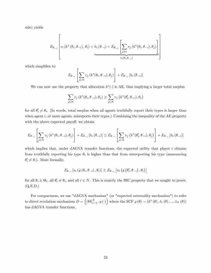
E��i

2666664vi (k� (�i; ��i) ; �i) + hi (��i) + E��i24Xj 6=i

vj (k�(�i; ��i); �j)

35| {z }

ti(�i;��i)

3777775which simpli�es to

E��i

24Xj2N

vj (k�(�i; ��i); �j)

35+ E��i [hi (��i)]We can now use the property that allocation k�(�) is AE, thus implying a larger total surplusX

j2Nvj (k

�(�i; ��i); �j) �Xj2N

vj�k�(�0i; ��i); �j

�for all �0i 6= �i. (In words, total surplus when all agents truthfully report their types is larger thanwhen agent i, or more agents, misreports their types.) Combining the inequality of the AE property

with the above expected payo¤, we obtain

E��i

24Xj2N

vj (k�(�i; ��i); �j)

35+ E��i [hi (��i)] � E��i24Xj2N

vj�k�(�0i; ��i); �j

�35+ E��i [hi (��i)]which implies that, under dAGVA transfer functions, the expected utility that player i obtains

from truthfully reporting his type �i is higher than that from misreporting his type (announcing

�0i 6= �i). More formally,

E��i [ui (g (�i; ��i) ; �i)] � E��i�ui�g��0i; ��i

�; �i��

for all �i 2 �i, all �0i 6= �i, and all i 2 N . This is exactly the BIC property that we sought to prove.(Q.E.D.)

For compactness, we use "dAGVA mechanism" (or "expected externality mechanism") to refer

to direct revelation mechanism D =�(�)Ni=1 ; g (�)

�where the SCF g (�) = (k� (�) ; t1 (�) ; :::; tN (�))

has dAGVA transfer functions.

24

8.3.1 dAGVA and Budget Balance

We can easily show that a proper choice of the hi (��i) function yields a dAGVA mechanism that

is strict BB, i.e.,Pi2N ti (�) = 0. In particular, consider a transfer

ti (�i; ��i) = E��i

24Xj 6=i

vj (k�(�i; ��i); �j)

35| {z }

"i(�i)

+

�� 1

N � 1

�Xj 6=i

"j (�j)| {z }hi(��i)

which can be rewritten as

ti (�i; ��i) = "i (�i)�1

N � 1Xj 6=i

"j (�j)

Summing over all i 2 N on both sides yields

Xi2N

ti (�i; ��i) =Xi2N

"i (�i)�1

N � 1Xi2N

Xj 6=i

"j (�j)| {z }Pi2N (N�1)"i(�i)

=Xi2N

"i (�i)�N � 1N � 1

Xi2N

"i (�i) = 0

Therefore, we obtain Xi2N

ti (�i; ��i) = 0

as required for strict BB. (Q.E.D.)

Example of dAGVA and strict BB. Consider a setting with three agents N = f1; 2; 3g.According to the above transfer function that guarantees strict BB, we have

ti (�i; ��i) = "i (�i)�1

2["j (�j) + "l (�l)] for every agent k 6= l 6= i

You can easily check that

3Xi=1

ti (�i; ��i) = "1 (�1)�1

2["2 (�2) + "3 (�3)] + "2 (�2)�

1

2["1 (�1) + "3 (�3)] + "3 (�3)�

1

2["1 (�1) + "2 (�2)]

= "1 (�1) + "2 (�2) + "3 (�3)�1

2[2"1 (�1) + 2"3 (�3) + 2"2 (�2)] = 0

Example of dAGVA - Bilateral trade. Consider a seller with equaly likely valuations

�1 = f10; 20g and a buyer with equaly likely valuations �2 = f10; 20g. Every agent i simultaneouslyand independently announces his type �i, and trade occurs if and only if �1 � �2 (the buyer�s

25

announced valuation �2 is weakly larger than that of the seller), which entails an allocation function

k� (�1; �2) that is AE.

Let us next �nd the valuation function for each pro�le of types (�1; �2). In particular, for the

seller,

v1 (k� (10; 10) ; 10) = �10; v1 (k

� (20; 10) ; 20) = 20

v1 (k� (10; 20) ; 10) = �10; v1 (k

� (20; 20) ; 20) = �20

and for the buyer,

v2 (k� (10; 10) ; 10) = 10; v2 (k

� (20; 10) ; 10) = 0

v2 (k� (10; 20) ; 20) = 20; v2 (k

� (20; 20) ; 20) = 20

Intuitively, when the announcement of buyer and seller is 10, trade occurs, entailing a loss

(gain) of 10 for the seller (buyer, respectively) gross of transfers, i.e., v1 = �10 but v1 = 10. If,

instead, the seller announces a valuation of 20 while the buyer announces a lower valuation of 10,

i.e., (20; 10), trade does not take place, entailing that the seller keeps the object with valuation

v1 = 20 while the buyer�s is v2 = 0.5

We can now compute the "i (�i) values, re�ecting the expected externality of every agent i.

First, for the seller the values of "1 (�1) are

"1(10) =1

2v2 (k

�(10; 10); 10) +1

2v2 (k

�(10; 20); 20) =1

2(10 + 20) = 15

"1(20) =1

2v2 (k

�(20; 10); 10) +1

2v2 (k

�(20; 20); 20) =1

2(0 + 20) = 10

Similarly, for the buyer (agent 2), the values of "2 (�2) are

"2 (10) =1

2(�10) + 1

2(20) = �5

"2 (20) =1

2(�10) + 1

2(�20) = �15

Therefore, the transfers for the seller become

t1 (10; 10) = "1 (10)� "2 (10) = 15� (�5) = 20

t1 (10; 20) = "1 (10)� "2 (20) = 15� (�15) = 0

t1 (20; 10) = "1 (20)� "2 (10) = 10� (�5) = 15

t1 (20; 20) = "1 (20)� "2 (20) = 10� (�15) = 255 In the opposite case, where the seller announces a valuation of 10 while the buyer announces a higher valuation

of 20, i.e., (10; 20), trade takes place, yielding a loss for the seller of v1 = �10 and a gain for the buyer�s of v2 = 20.

26

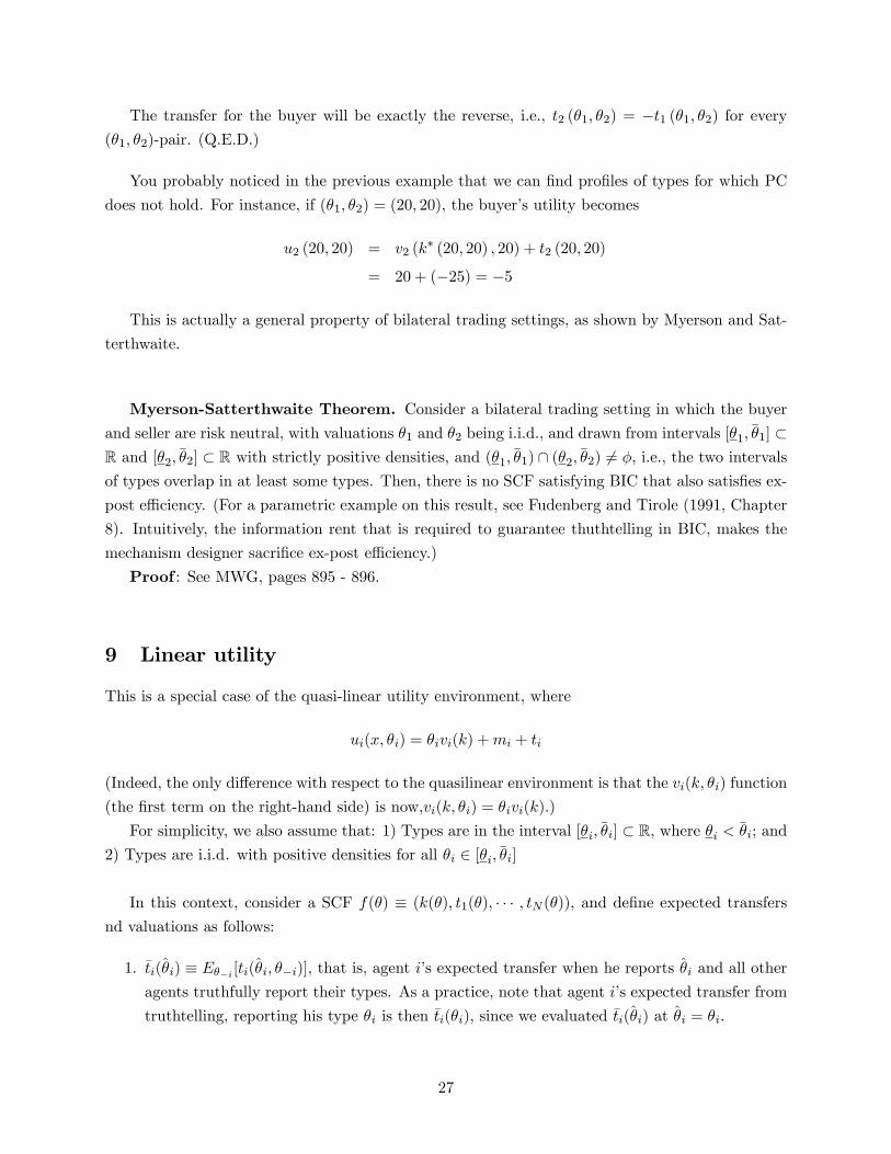
The transfer for the buyer will be exactly the reverse, i.e., t2 (�1; �2) = �t1 (�1; �2) for every(�1; �2)-pair. (Q.E.D.)

You probably noticed in the previous example that we can �nd pro�les of types for which PC

does not hold. For instance, if (�1; �2) = (20; 20), the buyer�s utility becomes

u2 (20; 20) = v2 (k� (20; 20) ; 20) + t2 (20; 20)

= 20 + (�25) = �5

This is actually a general property of bilateral trading settings, as shown by Myerson and Sat-

terthwaite.

Myerson-Satterthwaite Theorem. Consider a bilateral trading setting in which the buyerand seller are risk neutral, with valuations �1 and �2 being i.i.d., and drawn from intervals [�1; ��1] �R and [�2; ��2] � R with strictly positive densities, and (�1; ��1) \ (�2; ��2) 6= �, i.e., the two intervalsof types overlap in at least some types. Then, there is no SCF satisfying BIC that also satis�es ex-

post e¢ ciency. (For a parametric example on this result, see Fudenberg and Tirole (1991, Chapter

8). Intuitively, the information rent that is required to guarantee thuthtelling in BIC, makes the

mechanism designer sacri�ce ex-post e¢ ciency.)

Proof : See MWG, pages 895 - 896.

9 Linear utility

This is a special case of the quasi-linear utility environment, where

ui(x; �i) = �ivi(k) +mi + ti

(Indeed, the only di¤erence with respect to the quasilinear environment is that the vi(k; �i) function

(the �rst term on the right-hand side) is now,vi(k; �i) = �ivi(k).)

For simplicity, we also assume that: 1) Types are in the interval [�i; ��i] � R, where �i < ��i; and2) Types are i.i.d. with positive densities for all �i 2 [�i; ��i]

In this context, consider a SCF f(�) � (k(�); t1(�); � � � ; tN (�)), and de�ne expected transfersnd valuations as follows:

1. �ti(�i) � E��i [ti(�i; ��i)], that is, agent i�s expected transfer when he reports �i and all otheragents truthfully report their types. As a practice, note that agent i�s expected transfer from

truthtelling, reporting his type �i is then �ti(�i), since we evaluated �ti(�i) at �i = �i:

27

2. �vi(�i) � E��i [vi(�i; ��i)], that is, agent i�s expected valuation when he reports �i and all

other agents truthfully report their types. Again, we can then express his expected value

from truthtelling as �vi(�i).

3. ui(�ij��i) � E��i [ui(f(�i; ��i); �i)j�i] = �i�vi(�i) + �ti(�i), that is, agent i�s expected utility (ina linear environment) when he reports �i while all other agents truthfully report their types.

Finally, if agent i truthfully reports his type �i, i.e., �i = �i; his expected utility becomes

ui(�) = ui(�ij�i) = �i�v(�i) + �ti(�i)

We next present under which conditions a SCF in this linear environment satis�es BIC; a result

originally presented by Myerson.

9.1 Myerson Characterization Theorem

In a linear environment, a SCF is BIC if and only if for every agent i 2 N ,

1. �vi(�i) is nondecreasing in �i, and

2. Function vi(�i) can be expressed as

vi(�i) = vi(�i) +

Z �i

�i

�vi(s) ds for all �i 2 �i

Proof : See MWG, pp. 888-889.

Intuitively, we can identify all SCFs satisfying BIC in two steps: First, identify allocation

functions k(�) that lead every agent i�s expected bene�t function �vi(�i) to be weakly increasing in

his type �i; second, among these allocation functions, choose the expected transfer function �ti(�i)

that entails an expected utility which can be expressed in terms of the second condition of the

theorem. Substituting for vi(�i) in the above condition yields an expected transfer �ti(�i) of

�ti(�i) = �ti(�i) + �i�vi(�i)� �i�vi(�i) +Z �i

�i

�vi(s) ds

for some constant �ti(�i).

Since many studies in the auction theory and industrial organization consider linear environ-

ments for simplicity, Myerson�s characterization result has been applied to many applications. We

next present one of the most famous applications, in the auction theory, to show that, under rela-

tively general conditions, the expected revenue from selling an object using di¤erent auction formats

would coincide.

28

9.2 Revenue equivalence theorem

Consider I � 2 risk neutral bidders (so we operate in an environment of linear utility functions)

whose types satisfy �i 2 [�i; ��i], where �i 6= ��i and �i(�) > 0 for all �i 2 [�i; ��i] with independentdistribution of valuations among buyers. If the BNEs of two auction formats (e.g., the �rst- and

second-price auction) yield, for all pro�les of types � = (�1; � � � ; �I),

a) The same assignment rule (y1(�); y2(�); � � � ; yI(�)); and

b) The same value of u1(�1), u2(�2), � � � , uI(�I), where ui(�i) is the expected utility for buyer iif truthfully revealing his type when everybody else is also truthfully revealing his type. Then

the seller�s expected revenue is the same in both auction formats.

Proof : From the Revelation Principle we have that the SCF that implements the BNE of any

auction format is BIC.

We know that the seller�s expected revenue is given by the sum of expected transfers, i.e.,PIi=1E[��ti(�i)]. We initially �nd E[��ti(�i)]

E[��ti(�i)] =Z ��i

�i

��ti(�i)�i(�i) d�i

Since ui(�i) = �yi(�i)�i + �ti(�i) in this this linear environment, we can solve for the expected

transfer �ti(�i); which yields �ti(�i) = ui(�i) � �yi(�i)�i. Multiplying by �1 on both sides, we obtain��ti(�i) = �yi(�i)�i � ui(�i), which implies that the above expression becomes

E[��ti(�i)] =Z ��i

�i

[�yi(�i)�i � vi(�i)]| {z }��ti(�i)

�i(�i) d�i

and since ui(�i) = ui(�i) +R �i�i�y(s) ds, then E[��ti(�i)] becomes

E[��ti(�i)] =Z ��i

�i

266664�yi(�i)�i � vi(�i)�Z �i

�i

y(s) ds| {z }ui(�i)

377775�i(�i) d�i

Taking ui(�i) out of the integral operator, yields

E[��ti(�i)] =Z ��i

�i

"�yi(�i)�i �

Z �i

�i

y(s) ds

#�i(�i) d�i � ui(�i) (A)

29

Applying integration by parts in term (A), we obtain6:

Z ��

�

Z �i

�i

[yi(s) ds]�i(�i) d�i =

Z ��i

�i

�yi(�i) d�i �Z ��i

�i

�yi(�i)�i(�i) d�i

=

Z ��i

�i

�yi(�i)(1� �i(�i)) d�i

Substituting this result inside expression (A) yields:

E[��ti(�i)] =Z ��i

�i

��yi(�i)�i � �yi(�i)

1� �i(�i)�i(�i)

��i(�i) d�i

=

Z ��i

�i

�yi(�i)

��i �

1� �i(�i)�i(�i)

��i(�i) d�i � ui(�i)

which represents the expected transfer from bidder i: Finally, summing over all I bidders, we obtain7

IXi=1

E[��ti(�i)] =Z ��i

�i

� � �Z ��I

�I

IXi=1

�yi(�i)

��i �

1� �i(�i)�i(�i)

� IYi=1

�i(�i) d�I � � � d�i �IXi=1

ui(�i)

Therefore, if the BNE of two di¤erent auction formats have: (1) the same probabilities of assign-

ing the object to each bidder, (y1(�i); � � � ; yI(�I)); and (2) the same values for u1(�1); � � � ; uI(�I)we can easily see by the above expression that they will generate the same expected revenue for

the seller. (Q.E.D.)

Example: The FPA and SPA satisfy the conditions in this theorem since: (1) The allocation

rule in both auctions coincides, i.e., the bidder submitting the highest bid receives the object; and

(2) The expected utility of the bidder with the lowest valuation, ui(�i), when truthfully reporting

his type �i, coincides in both auctions (it is zero in both auction formats). Hence, the FPA and

the SPA generate the same revenue for the seller.

(Recall that we showed the Revenue Equivalence Theorem in our study of Auction Theory, but

for the speci�c case of uniformly distributed valuations, i.e., �i � U [0; 1] for all i 2 N . Now weshowed the same result under more general conditions, as we allowed for �i � [�i; ��i] where �i < ��iand �i(�) > 0 for all �i, where densities �i(�) are i.i.d.)

6 In order to apply integration by parts, a common trick is to �rst recall the derivative of the product of twofunctions f(x) and g(x) : (f:g)0 = f 0g + fg0; or alternatively fg0 = (f:g)0 � f 0g: Intergrating on both sides yieldsRfg0dx = fg �

Rf 0gdx: For our current example, let h(x) =

R �i�iyi(s)ds; g

0(x) = 'i(�i)d�i; h0(x) = yi(�i) and

g(x) = �i(�i): Plugging these functions are rearranging yields the above result.7 In this expression, we moved the summation signs inside the integral because types (�1; :::; �I) are independently

distributed.

30

10 Optimal Bayesian Mechanism

Let us now put ourselves in the shoes of mechanism designer, e.g., the seller of an object in an

auction, or a regulatory agency that does not observe the production cost of �rms in the regulated

industry. As mechanism designers, we now seek to select a feasible SCF that maximizes a certain

objective function, such as welfare or total revenue. But, what do we mean when we say �feasible

SCF�in the context? We focus on those SCF satisfy both BIC and IR (individual rationality, or

voluntary participation), and denote them as

F � = FBIC \ FIR

where FBIC = ff : �! X : f(�) is BICg, and FIR = ff : �! X : f(�) is IRg.Our goal will then be to select, among all feasible SCFs, the most e¢ cient SCFs (which guaran-

tees that we cannot achieve Pareto improvements by choosing a di¤erent SCF, as described below).

Before we start with the social planner�s problem, let�s de�ne three versions of e¢ ciency in SCFs:

ex-ante, interim, and ex-post e¢ ciency.

Ex-ante e¢ ciency: SCF f(�) 2 F is ex-ante e¢ cient if there is no other SCF f(�) 2 F that

yields

ui(f) � ui(f) for all i 2 N; and

ui(f) > ui(f) for at least one individual

That is, every agent i�s expected utility from the SCF f(�) is, before knowing his own type �i,weakly larger than from any other SCF f(�) 6= f(�).

Interim e¢ ciency: SCF f(�) 2 F is interim e¢ cient if there is no other SCF f(�) 2 F that

yields

ui(f j�i) � ui(f j�i) for all i 2 N; and all �i 2 �iui(f j�i) > ui(f j�i) for at least one individual and one of his types �i

In words, the expected utility that every individual i obtains, after learning his type �i, is

weakly larger with SCF f(�) than with any other SCF f(�) 6= f(�).

Ex-post e¢ ciency: SCF f(�) 2 F is ex-post e¢ cient if there is no other SCF f(�) 2 F that

yields

ui(f ; �) � ui(f; �) for all i 2 N; and all � 2 �

ui(f ; �) > ui(f; �) for some individual i and some pro�le � 2 �

31

That is, once all players� types have been revealed, the utility (not expected) that player i

obtains from SCF f(�) is weakly larger than from any other SCF f(�) 6= f(�).We will next search for optimal mechanisms. That is, SCFs that maximize the objective function

of the mechanism designer subject to the constraint that the SCFs we consider must be feasible, i.e.,

f(�) 2 F �, and thus satisfy BIC and IR. In particular, we conduct that search in two applications:�rst, in the principal-agent problem, and then in the design of monopoly licences in an industry.

10.1 The Principal-Agent problem using Mechanism Design

Consider the principal-agent problem from previous chapters, but allow for a continuum of types

for the agent (rather than only two), in particular, � 2 [�; ��], where � < �� < 0, and where � is

drawn from a cdf �(�) with positive density �(�) > 0 for all � 2 [�; ��]. In addition, assume that

� � 1� �(�)�(�)

is nondecreasing in �

(We return to the assumption below.) The agent�s utility function is

u(e; t1; �) = t1 + � � g(e)

where recall that � < �� < 0, i.e., the realization of � is always negative, implying that the agent�s

disutility of e¤ort, g(e); enters negatively in his utility function. Furthermore, the disutility of e¤ort

g(�) satis�es g(0) = 0, g(e) > 0 for all e > 0, g0(e) > 0 and g00(e) > 0 for all e > 0. Intuitively, asmaller � (more negative parameter since � < �� < 0 by de�nition) implies a larger disutility from

a given amount of e¤ort e > 0.

The principal�s (agent 0) utility is

u0(e; t0) = v(e) + t0

where v0(e) > 0, and v00(e) < 0 for all e � 0. Intuitively, a larger e¤ort by the agent increases the�rm�s pro�ts, but a decreasing rate.

Since the principal is considering SCFs that satisfy BIC, the agent must be provided incentives

to truthfully reveal his type. We can then invoke the Revelation Principle so that the principal,

rather than designing an IRM, can more easily design a DRM in which the agent is induced to

truthfully announce his type �, and then the principal maps it into the SCF

f(�) = (e(�); t0(�); t1(�))

where e(�) plays the role of the outcome function, thus being analogous to k(�) in our previous

discussions; while t0(�) and t1(�) are transfer functions to the principal and the agent, respectively.

For simplicity, we assume that all transfers to the agent originate from the principal, i.e., �t0(�) =

32

t1(�) for all �, which helps us reduce the three elements of the above SCF to only two, i.e., f(�) =

(e(�); t1(�)).Since the principal�s objective function is v(e)+t0 = v(e)�t1, his expected utility maximization

problem becomes to choose a SCF f(�) = (e(�); t1(�)) that solves

max(e(�);t1(�))

E� [v(e(�))� t1(�)]

subject to f(:) being feasible, i.e., f(�) 2 F �

Since agent�s utility is linear, we can use some of the notations presented in the section on linear

utility to simplify our problem. In particular, let e play the role of e in previous sections, so that

we can use g(e) rather than v1(k) and, hence, use g(e(�)) rather than v1(k):We can then represent

the agent�s expected utility from truthfully reporting his type, �; as

U1(�) = t1(�) + � � g(e(�))

Solving for transfer t1(�); yields

t1(�) = U1(�)� � � g(e(�))

Plugging t1(�) in the principal�s objective function, we obtain

maxe(�);U1(�)

E�[v(e(�))�U1(�) + �g(e(�))| {z }�t1(�)

]

subject to f 2 F �

(Note the change in choice variables, from (e(�); t1(�)) to (e(�); U1(�)), since t1(�) is now absent fromthe program.)

How can we express the feasibility constraint, f(:) 2 F �, in a more tractable way? Feasibil-

ity entails both BIC and IR. For the �rst property, recall that, from Myerson�s characterization

theorem, in a linear environment, a SCF f(�) is BIC if and only if :

1. �U1(�) is nondecreasing in �. In our principal-agent context, that entails g(e(�)) being nonde-

creasing in �. But since g0(e) > 0 by de�nition, this amounts to the agent�s e¤ort e(�) being

nondecreasing in his type �.

2. Ui(�i) = Ui(�i) +R �i�i�vi(s) ds for all �i, which in our principal-agent context implies that

U1(�) = U1(�) +R �� g(e(s)) ds for all �.

From the above conditions, we know how to express BIC, but how can we express IR? That

property is actually easier to represent than BIC. In particular, for IR we need that

U1(�) � �u for all �

33

That is, the expected utility that the agent obtains from participating, when he truthfully reveals

his type �, is larger than his reservation utility level �u.

Summarizing, the principal�s problem can be expressed as follows

maxe(�);U1(�)

E� [v(e(�))� U1(�) + �g(e(�))]

subject to 1) e(�) is nondecreasing in �

2) U1(�) = U1(�) +

Z �

�g(e(s)) ds for all �

3) U1(�) � �u for all �

where the �rst two constraints guarantee BIC (thanks to Myerson�s characterization theorem), and

the third constraint guarantees IR.

Before taking FOCs, let�s try to simplify our problem. First, note that if constraint (2) holds,

then U1(�) � U1(�) sinceR �� g(e(s)) ds is positive for all �. Hence, constraint (3) would also hold

if and only if it holds for the agent with the lowest type, �; i.e., U1(�) � �u. We can then replace

constraint (3) for its version evaluated at the lowest type � = �,

U1(�) � �u

which we denote as constraint (3)�. Second, we can substitute U1(�) in the objective function from

constraint (2), yielding a slightly reduced program:

maxe(�);U1(�)

E�

266664v(e(�))�U1(�)�Z �

�g(e(s)) ds| {z }

�U1(�)

+�g(e(�))

377775subject to

1) e(�) is nondecreasing in �

3)0 U1(�) � �u for all �

(Note the change in choice variables, from U1(�) to U1(�) since now U1(�) is absent from objective

function and constraints.)

Expanding the integral, in the objective function yields

maxe(�);U1(�)

Z ��

�[v(e(�))+�g(e(�))]�(�) d� �

Z ��

�

Z �

�[g(e(s)) ds]�(�) d� �

Z ��

�U1(�)�(�) d�

subject to

1) e(�) is nondecreasing in �

3)0 U1(�) � �u for all �

34

Note that U1(�) is a constant, and thus the last term of the objective function becomes

Z ��

�U1(�)�(�) d� = U1(�)

Likewise, we can use integration by parts to simplify the second term of the principal�s objective

function.8 Applying integration by parts on the second term of the objective function, yieldsZ ��

�

Z �

�[g(e(s)) ds]�(�) d� =

Z ��

�[g(e(�))� �(�)g(e(�))] d�

=

Z ��

�[g(e(�))(1� �(�))] d�

We can now substitute our simpli�cation back into the second term of the objective function,

we obtain

maxe(�);U1(�1)

Z ��

�[v(e(�))+�g(e(�))]�(�) d� �

Z ��

�[g(e(�))(1� �(�))] d� � U1(�)

=

Z ��

�[[v(e(�)) + �g(e(�))]�(�) d� � g(e(�))(1� �(�))] d� � U1(�)

subject to

1) e(�) is nondecreasing in �

3)0 U1(�) � �u for all �

and factoring out g(e(�)) yields

maxe(�);U1(�)

Z ��

�

�v(e(�)) +

�� � 1� �(�)

�(�)

�g(e(�))

��(�)d� � U1(�)

subject to

1) e(�) is nondecreasing in �

3)0 v1(�) � �u for all �

Finally, note that the PC constraint (3)�must hold with equality; otherwise the principal could

still reduce U1(�) furthermore and extract more surplus from the agent with the lowest �. We can

8Recall that the formula for integrations by partsRh(x)g0(x) dx = h(x)g(x) �

Rg(x)h0(x) dx and let h(x) =R ��

�[g(e(�)) d�], h0(x) = g(e(�))d�, g(x) = �(�), and g0(x) = �(�)d�.where �(�) represents the cdf of the distribution.

Applying integration by parts on the second term of the objective function, yieldsZ ��

�

Z �

�

[g(e(s)) ds]| {z }h

�(�) d�| {z }g0

=

�Z �

�

[g(e(s)) ds]

�| {z }

h

�(�)j���| {z }g

�Z �

�

�(�)|{z}g

g(e(�))| {z }h0

d�

35

then use U1(�) = �u into the objective function to obtain the following reduced program:

maxe(�)

Z ��

�

�v(e(�)) +

�� � 1� �(�)

�(�)

�g(e(�))

��(�)d� � �u

subject to 1) e(�) is nondecreasing in �

which has only one choice variable, e(�), since neither the objective function nor the (single) con-straint depends on U1(�) any more.

As in similar applications, we can now solve the unconstrained program, i.e., ignoring constraint

(1), and later on show that our results indeed satisfy constraint (1). Taking FOC with respect to

e yields

v0(e(�)) +

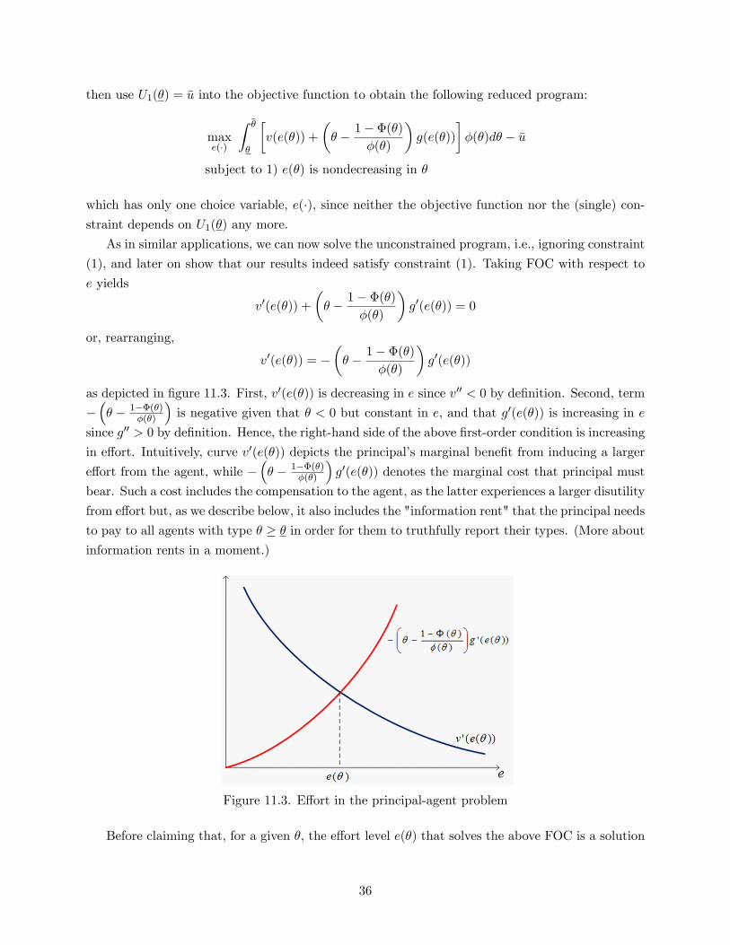
�� � 1� �(�)

�(�)

�g0(e(�)) = 0

or, rearranging,

v0(e(�)) = ��� � 1� �(�)

�(�)

�g0(e(�))

as depicted in �gure 11.3. First, v0(e(�)) is decreasing in e since v00 < 0 by de�nition. Second, term

��� � 1��(�)

�(�)

�is negative given that � < 0 but constant in e, and that g0(e(�)) is increasing in e

since g00 > 0 by de�nition. Hence, the right-hand side of the above �rst-order condition is increasing

in e¤ort. Intuitively, curve v0(e(�)) depicts the principal�s marginal bene�t from inducing a larger

e¤ort from the agent, while ��� � 1��(�)

�(�)

�g0(e(�)) denotes the marginal cost that principal must

bear. Such a cost includes the compensation to the agent, as the latter experiences a larger disutility

from e¤ort but, as we describe below, it also includes the "information rent" that the principal needs

to pay to all agents with type � � � in order for them to truthfully report their types. (More about

information rents in a moment.)

Figure 11.3. E¤ort in the principal-agent problem

Before claiming that, for a given �, the e¤ort level e(�) that solves the above FOC is a solution

36

of the principal�s problem, we still need to check if it satis�es the (so far ignored) constraint (1).

In particular, does the agent�s e¤ort e(�) weakly increase in �?

Yes! Since � � 1��(�)�(�) is nondecreasing in � by assumption, the application of the implicit

function theorem yields that e(�) is weakly increasing in �. In particular, before di¤erentiating the

above FOC with respect to �; let us rewrite it as follows:

v0(e(�)) + J(�)g0(e(�)) = 0

where, for compactness, J(�) = � � 1��(�)�(�) : We can now di¤erentiate with respect to �; and apply

the chain rule to obtain

v00(e(�)) � e0(�) + J 0(�)g0(e(�)) + J(�)g00(e(�))e0(�) = 0

where J 0(�) � @J(�)@� . Factoring out e

0(�) we obtain

e0(�)�v00(e(�)) + J(�)g00(e(�))

�= �J 0(�)g0(e(�))

or,

e0(�) = � J 0(�)g0(e(�))

v00(e(�)) + J(�)g00(e(�))= � (+)(+)

(�) + (�)(+) = �(+)

(�) = (+)

In the numerator, J 0(�) > 0 holds by assumption, as well as g0(�) > 0. In the denominator, v00 < 0,

J(�) < 0, � < 0; and g00 > 0 all hold by de�nition.

Complete information. If the principal was, instead, perfectly informed about the agent�stype, �, his problem would be

maxe(�);t1(�)

v(e(�))� t1(�)

subject to t1(�) + �g(�) � �u; for all �

which, as usual, is only subject to the voluntary participation constraint of the agent (PC), but

does not require BIC in order to induce the agent to truthfully report his type, �, as the principal

now knows this information. The PC constraint must bind (otherwise the principal could lower

the transfer t1(�) to the agent), impying that we can use t1(�) = �u� �g(e(�)), and plug it into theprincipal�s objective function as follows

maxe(�)

v(e(�))��u+ �g(e(�))| {z }�t1(�)

which only includes one choice variable. Taking FOC with respect to e yields

v0�(e(�)) + �g(e�(�))

37

where e�(�) represents the pro�t-maximizing e¤ort function under complete information. Figure

11.4 depicts this e¤ort level by separately examining the two terms of the above FOC.

Figure 11.4. Principal-agent model - Comparison

For comparison purposes, the �gure also plots ��� � 1��(�)

�(�)

�g0(e) from the FOCs under in-

complete information (recall that the LHS of the FOC under complete information coincide, but

the RHS di¤er, as depicted in the two upward sloping lines of �gure 11.4). In particular,

��� � 1� �(�)

�(�)

�> ��

which simpli�es to1� �(�)�(�)

> 0

given that �(�) > 0 and �(�) 2 [0; 1] for all �. Therefore, the e¤ort level that the principal inducesunder incomplete information is smaller than under complete information. This is true for all

agents with types � < ��, but not for the most e¢ cient type of worker, � = ��, since evaluating the

FOC under incomplete information at � = �� yields

v0(e(��)) +

��� � 1� �(

��)

�(��)

�g0(e(��)) = 0

where ��� 1��(��)�(��)

= ��� 1�1�(��)

= �� since �(�) = 1 (i.e., full cumulated probability at the highest type).

Therefore, the FOC simpli�es to

v0(e(��)) + ��g0(e(��)) = 0

which coincides with the FOC under complete information for � = ��. This is a usual result:

� �No distortion at the top�: The �top� agent (in this context, the agent with the smallestdisutility of e¤ort, � = ��), su¤ers no distortion relative to complete information strategies.

38

His utility level in equilibrium also coincides in both information contexts.

� �Downward distortion�for all other types of agents, � < ��, since their e¤orts are lower underincomplete information than under complete information, e�(�) < e(�).

Example: Assume that types are uniformly distributed, �i � U [0; 1], then the cdf �(�) = �

and its density �(�) = 1, which yields

J(�) = � � 1� �(�)�(�)

= � � 1� �1

= 2� � 1

which is nondecreasing in �. In addition, assume that the principal�s return from e¤ort (e.g.,

production) is given by concave function v(e) = ln e, where v0(e) = 1e ; and that the agent�s disutility

of e¤ort is represented by a convex function g(e) = e2, where g0(e) = 2e. We can then evaluate the

FOC under incomplete information obtaining

1

e+ (2� � 1)2e = 0

which, solving for e, yields an optimal e¤ort of

eI:I:(�) =1

(2� 4�)1=2

which is indeed increasing in �. �

Virtual valuations and Information rents. The term J(�) = �� 1��(�)�(�) , or more generally,

J(�) = �� 1�F (�)f(�) , is often referred to as the principal�s �virtual valuation�of assigning more e¤ort

to an agent with type �. Consider the e¤ect of increasing more e¤ort to agent �. On one hand,

such higher e¤ort allows the principal to increase his pro�ts by v0(e). However, in order to induce

such additional e¤ort the agent must now receive a larger transfer to compensate for his larger

disutility of e¤ort, � �g0(e). Until this point we just described the trade-o¤ that the principal wouldexperience under a complete information setting. Under incomplete information, however, a new

e¤ect emerges. In particular, from constraint (2), an increase in the e¤ort from agent � entails a

larger transfer to all types above �. Speci�cally, since their probability mass is 1� F (�), the totalexpected cost of increasing the e¤ort from agent � is

[�f(�)� (1� F (�))] g0(e(�))

which, dividing by f(�), can be expressed as�� � 1� F (�)

f(�)

�g0(e(�))

39

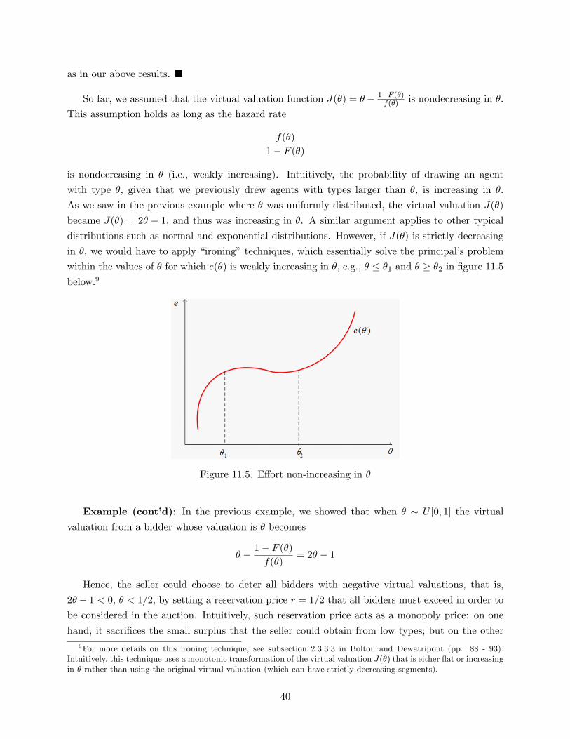
as in our above results. �

So far, we assumed that the virtual valuation function J(�) = �� 1�F (�)f(�) is nondecreasing in �.

This assumption holds as long as the hazard rate

f(�)

1� F (�)

is nondecreasing in � (i.e., weakly increasing). Intuitively, the probability of drawing an agent

with type �, given that we previously drew agents with types larger than �, is increasing in �.

As we saw in the previous example where � was uniformly distributed, the virtual valuation J(�)

became J(�) = 2� � 1, and thus was increasing in �. A similar argument applies to other typicaldistributions such as normal and exponential distributions. However, if J(�) is strictly decreasing

in �, we would have to apply �ironing�techniques, which essentially solve the principal�s problem

within the values of � for which e(�) is weakly increasing in �, e.g., � � �1 and � � �2 in �gure 11.5below.9

Figure 11.5. E¤ort non-increasing in �

Example (cont�d): In the previous example, we showed that when � � U [0; 1] the virtual

valuation from a bidder whose valuation is � becomes

� � 1� F (�)f(�)

= 2� � 1

Hence, the seller could choose to deter all bidders with negative virtual valuations, that is,

2�� 1 < 0, � < 1=2, by setting a reservation price r = 1=2 that all bidders must exceed in order tobe considered in the auction. Intuitively, such reservation price acts as a monopoly price: on one

hand, it sacri�ces the small surplus that the seller could obtain from low types; but on the other9For more details on this ironing technique, see subsection 2.3.3.3 in Bolton and Dewatripont (pp. 88 - 93).

Intuitively, this technique uses a monotonic transformation of the virtual valuation J(�) that is either �at or increasingin � rather than using the original virtual valuation (which can have strictly decreasing segments).

40

hand, it increases the surplus that the seller gets from higher types. Interestingly, such optimal

reservation price r = 1=2 does not depend on the number of bidders but on the distribution of their

valuations alone.10

In the case of asymetric cdfs, consider that bidder j has ex-ante higher types than bidder i.

More formally, their hazard rates satisfy

f j(�)

1� F j(�) <f i(�)

1� F i(�)

Then, cross multiplying1� F i(�)f i(�)

<1� F j(�)f j(�)

Multiplying both sides by �1 and adding � on both sides yields

� � 1� Fi(�)

f i(�)> � � 1� F

j(�)

f j(�)

That is, their virtual valuation satis�es J i(�) > J j(�), implying that the object is allocated to

agent i. Intuitively, the seller favors weak bidders in order to extract a larger surplus from strong

bidders.

10.2 Exercise - Optimal Auction of Monopoly Rights

Consider the following model based on the article by Dana and Spier (1994)11. A regulator sells

the monopoly right in an industry among two �rms, i = f1; 2g: Assume that the social planner�sobjective is to maximize social welfare:

W =Xi

�i + S + (�� 1)Xi

ti

where �j is the gross pro�t (pretransfer) of producer j; S denotes consumer surplus; � represents

the shadow cost of raising public funds through distortionary taxation, where � > 1; and ti is

transfer from the government to producer i.

The regulator determines which �rm (or �rms) obtain the production license, and the transfer

from every �rm i to the regulator, ti for all i = f1; 2g: Once one (or both) �rms obtain a productionlicense it freely determines its pro�t maximizing output. Each �rm privately observes its �xed cost

of production, �i; which is drawn from [�; �] with cdf �(:) and positive density �(�i) for all �i and all

i = f1; 2g: For simplicity, assume that �(�i)�(�i)is increasing in �i: Both �rms face a common marginal

cost c < 1; and increase demand function p(x) = 1 � x; which is common knowledge among allplayers.

10Alternatively, the seller could set an entry fee (a participation fee for the auction) high enough to make type� = r indi¤erent between participating and not participating.11Dana, J.D. and Spier, K.E. 1994. "Designing a private industry: Government auctions with endogenous market

structure." Journal of Public Economics. 53 (1). 127-147.

41

Complete Information: When the regulator observes the pro�le of � = (�1; �2); he �rst

evaluates the welfare emerging from each market structure, that is,

Monopoly W i(�) = Sm;i + �m;i(�) for every i = f1; 2g

Duopoly W d(�) = Sd + [�d;1(�) + �d;2(�)]

and chooses the transfers t = (t1; t2) and probabilities of implementing each market structure

p = (p1; p2; pd) that solves

maxt;p

p1(�)W 1(�) + p2(�)W 2(�) + pd(�)W d(�)� (1� �)[t1(�) + t2(�)]

subject to �m;i(�) � ti and

�d;i(�) � ti for all i = f1; 2g

If W i(�) � W d(�) for the observed pro�le of �; then the regulator sets pi(�) = 1 and reduces

transfer ti enough to guarantee the participation of �rm i; i.e., �m;i(�) = 0; entailing that the

above program reduces to

�(1� �)[�m;i + 0] + [�m;i(�) + Sm;i(�)] + 0 + 0

= Sm;i(�) + ��m;i for every i = f1; 2g

where �m;i = ti and �m;i(�) + Sm;i(�) =W i(�).

A similar argument applies to the case in which W i(�) < W d(�); where pd(�) = 1 and �d;1(�)+

�d;2(�) = t1 + t2; yielding a social welfare of

Sd;i(�) + �[�d;1(�) + �d;2(�)]

By employing the Revelation Principle we can restrict attention to truth-telling equilibrium in

direct-revelation mechanisms. Hence, the government mechanism ft; pg satis�es:

� transfer from each �rm ti(�1; �2) for all i = f1; 2g:

� probability of implementing each market structure pi(�1; �2); where j = f1; 2; dg where �1 and�2 are the announcements made by each �rm and p = (p1; p2; pd) 2 �3 indicates the proba-bility that �rm 1 obtains the monopoly license, or both �rms do in a duopoly, respectively.

Each �rm has prior beliefs about the other �rms�cost parameter given by �i(�i). Hence, �rm

1�s expected pro�t as a function of its reported cost �1 (which allows for �1 6= �1) and the true costof �rm 2, �2 is given by:

�1(�1j�) = E�2hp1(�1; �2) � �m;1(�1; �2) + pd(�1; �2) � �d;1(�1; �2)� t1(�1; �2)

i42

Intuitively, �rm 1 makes some pro�ts when it is given the monopoly right (which happens with

probability p1(�1; �2) and yields pro�ts of �m;1(�1; �2) thus depending on its true cost �1), or when

the regulator assigns production rights to both �rms, which happens with probability pd(�1; �2)

and yields duopoly pro�ts of �d;1(�1; �2): A similar argument applies to the expected pro�ts of �rm

2, when it announces �2; �2(�2j�): The social planner�s optimization problem is given by:

maxt;p

E�[(�� 1)[t1(�) + t2(�)] + p1(�)[�m;1(�) + Sm;1(�)]

+p2(�)[�m;2(�) + Sm;2(�) + pd(�)[�d;1(�) + �d;2(�) + Sd(�)] (1)

subject to (p1; p2; pd) 2 �3

�i(�ij�i) � �i(�ij�i) for all �i; �i 2 [�; �] and all i = 1; 2 (BIC)

�i(�ij�i) � 0 for all �i 2 [�; �] and all i = 1; 2 (IR)

The "virtual welfare" function corresponding to a monopoly awarded to �rm i is:

W i(�) = Sm;i(�) + ��m;i(�)| {z }welfare under complete inforamation

+ (�� 1)�m;ii (�)�(�i)

�(�i)| {z }plus the cost of inducing �rm i to reveal its private information

And the "virtual welfare" function corresponding to a duopoly is:

W d(�) = Sd(�) + �h�d;1(�) + �d;2(�)

i| {z }welfare under complete information

+ (�� 1)��d;11 (�)

�(�1)

�(�1)+ �d;22 (�)

�(�2)

�(�2)

�| {z }

cost of inducing both �rms to reveal their private information

Parametric example. The above analysis left results in a general format, but in this setting wehave information about the inverse demand function p(x) = 1�x and about total costs TC = �i+cx,where c < 1 represents marginal costs.

Monopoly: Under monopoly it is straight forward to �nd that the monopoly output of �rm i is

xm = 1�c2 , yielding a monopoly price p(x

m) = 1+c2 ; and monopoly pro�ts of

�m;i(�) = p(xm)xm � TC = 1 + c

2� 1� c2

� �i � c1� c2

=(1� c)24

� �i

43

Therefore, the "virtual welfare function" corresponding to a monopoly awarded to �rm i is:

W i(�) =(1� c)28| {z }CS

+�

�(1� c)24

� �i�

| {z }�m;i

+(�� 1)(�1)�(�i)�(�i)

for all i = 1; 2:

Note that the derivative of pro�ts with respect to. �i is �m;i = �1. If, for instance, �i is uni-formly distributed in [0; 1];�(�i) = �i and �(�i) = 1; reducing third term of the above expression

to (�� 1)(�1)�i = (1� �)�i:

Cournot Duopoly: Firm 1�s equilibrium output under duopoly is xi = 1�c3 ; yielding duopoly

pro�ts of:

�d;1 = p(x)x1 � TC =�1� 1� c

3� 1� c

3

�� 1� c3

� �1 � c1� c3

=

�1� c3

�2� �1

Hence, aggregate duopoly pro�ts are

�d;1 + �d;2 =

�1� c3

�2� �1 +

�1� c3

�2� �2 = 2

�1� c3

�2� �1 � �2

And, the associated consumer surplus, Sd(�); is:

Sd(�) =1

2

�1� 1 + 2c

3

�2� 2c3

=2(1� c)2

9

44

Therefore, the "virtual welfare function" corresponding to a duopoly is:

W d(�) =2(1� c)2

9| {z }CS

+�

�2(1� c)2

9� �1 � �2

�| {z }

�d;1+�d;2

+(�� 1)�(�1)�(�1)

�(�1)+ (�1)�(�2)

�(�2)

�

Similarly, as under monopoly, if �i ~ U [0; 1] for every �rm i = f1; 2g; the third term in the

above expression simpli�es to (�� 1)[��1� �2] = (1� �)(�1+ �2): Finally, the government awardsa monopoly to �rm i if the virtual welfare functions satisfy

W i(�) = maxnW 1(�); W 2(�); W d(�)

oand the government awards a duopoly if, instead, the duopoly yields a higher virtual welfare than

the monopoly to either �rm

W d(�) = maxnW 1(�); W 2(�); W d(�)

o

Numerical Example: Consider that the marginal cost is c = 14 , and that types are uniformly

distributed in [0; 1], so that �(�1) = �1 and �(�2) = �2. (Densities are, therefore, �(�1) = 1 and

�(�2) = 1:) Assume that the realization of �1 is �1 = 12 and that of �2 is �2 =

13 . Let us �rst

evaluate the virtual welfare functions of a monopoly awarded to �rm 1, W 1(�), to �rm 2, W 2(�),

or to both (in a duopoly), W d(�). In particular

45

W 1(�) =

�1� 1

4

�28

+ �

"�1� 1

4

�24

� 12

#+ (1� �)1

2

=9

128+ �

�9

64� 12

�+(1� �)2

=73

128� 5564�

W 2(�) =(1� 1

4)2

8+ �

"�1� 1

4

�24

� 13

#+ (1� �)1

3

=9

128+ �

�9

64� 13

�+(1� �)3

=155

384� 101192

�

W d(�) =2(1� 1

4)2

9+ �

"2�1� 1

4

�29

� 12� 13

#+ (�� 1)

�(�1) � 1

2+ (�1) � 1

3

�=1

8+ �

�1

8� 56

�� 56(�� 1)

=23

24� 3724�

They are all a function of the shadow cost of raising public funds, �. The next �gure depicts

the three virtual welfare functions, showing that, since � > 1 by de�nition, assigning the monopoly

rights to �rm 2 is welfare superior duopoly yields a larger welfare otherwise.

If, instead, we assume that �1 = 14 and �2 =

13 (i.e., reversing the realization of these parameters

46

across players), we obtain

W 1(�) =41� 46�128

, W 2(�) =73� 110�128

, and W d(�) =23� 37�24

thus entailing that, since � > 1 by de�nition, assigning the monopoly rights to �rm 1 yields a larger

welfare than the other alternatives.

11 Appendix 1:

Proposition: Under quasilinear preferences, SCF f(�) satis�es

Ex-post e¢ ciency() Allocative e¢ ciency + Budget balanced

Proof : We �rst show su¢ ciency, i.e., the ( line of implication, and we then demonstrate the

opposite line of implication ()). If f(�) satis�es allocative e¢ ciency (AE) and budget balanced(BB), then for every pro�le of types � 2 �,X

i2Nui (f(�); �i) =

Xi2N

ui (k(�); �i) +Xi2N

ti(�)

�Xi2N

ui(x; �i) +Xi2N

ti

=Xi2N

ui(x; �i)

The �rst equality uses quasilinearity in preferences, thus expanding ui(f(�); �i) into ui(k(�); �i)+

ti for each agent i. The subsequent inequality makes use of AE, which implies that k(�) generates

a larger social surplus than any other feasible outcome x 2 X. Finally, the last equality uses BB,i.e.,

Pi2N ti = 0.

Hence, reproducing the �rst and last elements of the above expression we obtainXi2N

ui (f(�); �i) �Xi2N

ui(x; �i); for all x 2 X

which coincides with the de�nition of ex-post e¢ ciency; as required.

Let us now show that ex-post e¢ ciency implies, separately, AE and BB. We approach both

proofs by contradiction in the next two claims.

Claim 1: If f(�) is not AE, then it is not ex-post e¢ cient.Proof: If f(�) is not AE, there must be at least one type pro�le �0 2 � and an alternative

47

allocation k0 2 K such that total surplus is larger with k0 than that with k(�)Xi2N

ui(k0; �) >

Xi2N

ui (k(�); �i)

This implies that there exists at least one agent j who is strictly better o¤ with allocation k0

than with k(�);

uj(k0; �j) > uj (k(�); �j)

Now, consider an alternative outcome x in which we implement k0 by giving agent j a larger

transfer than under f(�), that is

ti = ti(�) +�ui (k(�); �i)� ui(k0; �i)

�; for all i 6= j

tj = tj(�) +�uj (k(�); �j)� uj(k0; �j) + "

�; for agent j

Since vi (k(�); �i) = vi(k0; �i) for all i 6= j, the transfer we implemented coincides with the

original transfer, ti = ti(�), and thus

ui(k0; �i) = ui (f(�); �i) ; for all i 6= j

However, since uj(k0; �j) > uj (k(�); �j), the transfer we implemented for agent j is more gen-

erous than the original transfer, tj > tj(�), implying

uj(k0; �j) > uj (f(�); �j)

Therefore,Pi2N

ui(f(�); �i) <Pi2N

ui(k0; �i) entailing that the SCF f(�) is not ex-post e¢ cient, as

required. (Q.E.D. for Claim 1)

Claim 2: If f(�) is not BB, then it is not ex-post e¢ cient.Proof: If f(�) is not BB, then there must be at least one agent j such that he pays to the

system, tj(�) < 0. We can then consider a di¤erent outcome that leaves agent j better o¤ and no

agent worse o¤. In particular, outcome x has transfer functions

ti = ti(�) for all i 6= j

tj = tj(�) + " for agent j

Hence, f(�) is not ex-post e¢ cient. (Q.E.D. of Claim 2)

48