An introduction to Logic Programming Chapter 6. So far… The computational process was about...
108
An introduction to Logic Programming Chapter 6
-
Upload
ami-bailey -
Category
Documents
-
view
225 -
download
0
Transcript of An introduction to Logic Programming Chapter 6. So far… The computational process was about...
An introduction to Logic Programming
Chapter 6
2
So far…
• The computational process was about finding values
• And now for something completely different.
3
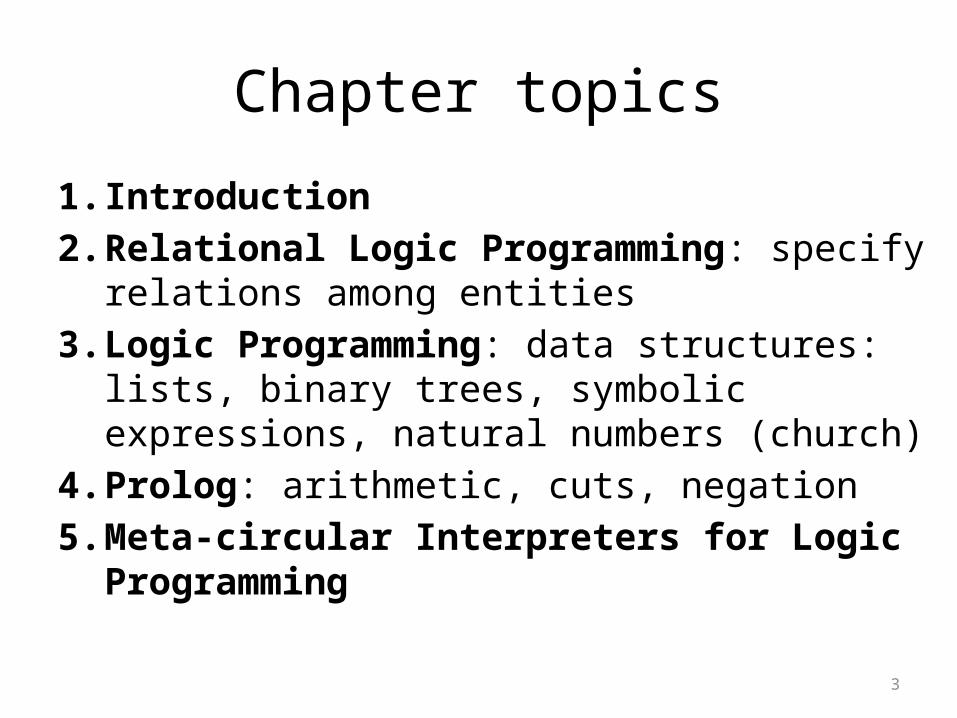
Chapter topics
1. Introduction2. Relational Logic Programming: specify relations
among entities3. Logic Programming: data structures: lists, binary
trees, symbolic expressions, natural numbers (church)
4. Prolog: arithmetic, cuts, negation5. Meta-circular Interpreters for Logic
Programming
4
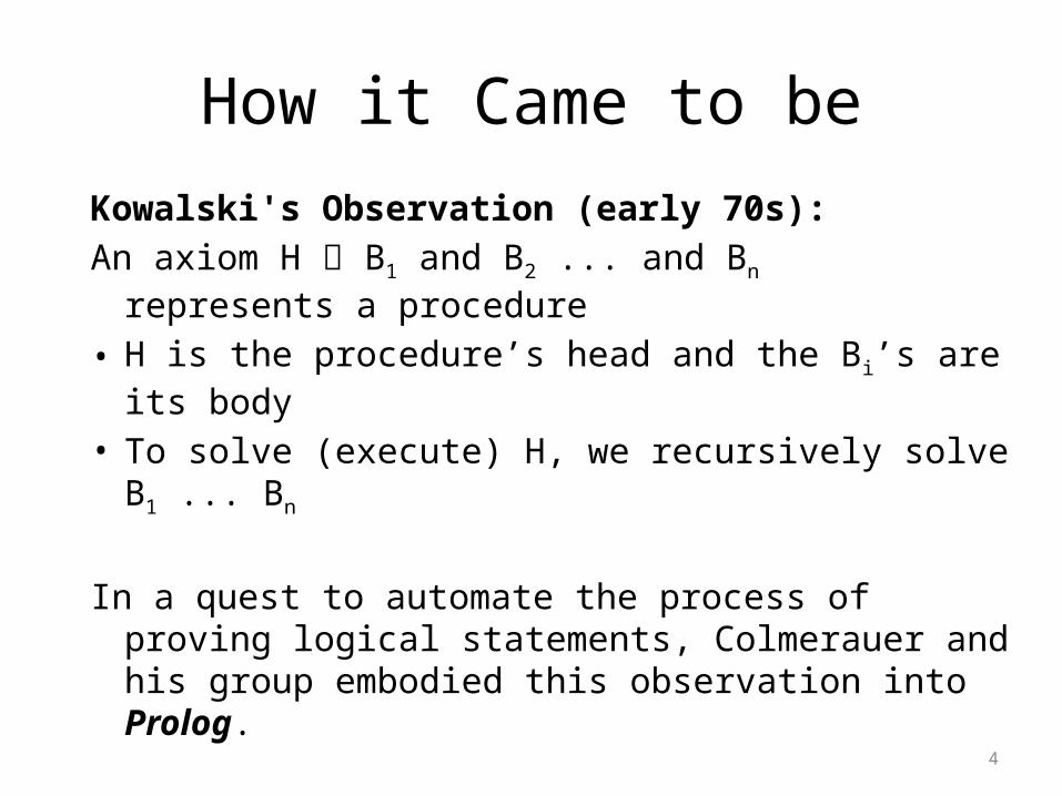
How it Came to be
Kowalski's Observation (early 70s):An axiom H B1 and B2 ... and Bn
represents a procedure • H is the procedure’s head and the Bi’s are its body
• To solve (execute) H, we recursively solve B1 ... Bn
In a quest to automate the process of proving logical statements, Colmerauer and his group embodied this observation into Prolog.
5
Actually two Prologs
• Pure logic programming– No types, no primitives.
• Full Prolog– Types, arithmetic primitives, data structures and
more
6
Logic Programming: Introduction
Every programming language has:• Syntax: set of formulas (facts and rules)• Semantics (set of answers to queries)• Operational Semantics (how to get an
answer):– Unification– Backtracking
7
Logic Programming: Introduction
• Mind switch:– Formula procedure declaration⇔– Query procedure call⇔– Proving computation⇔

8
Relational Logic Programming
• a computational model based on Kowalski's interpretation
• The Prolog language ('70) - contains RLP + additional programming features
9
Relational LP - Syntax• atomic formula:predicate_symbol(term1, ..., termn)
• predicate symbols start with lowercase• terms:– symbols (representing individual constants)– variables (start with uppercase or _ for anonymous)
10
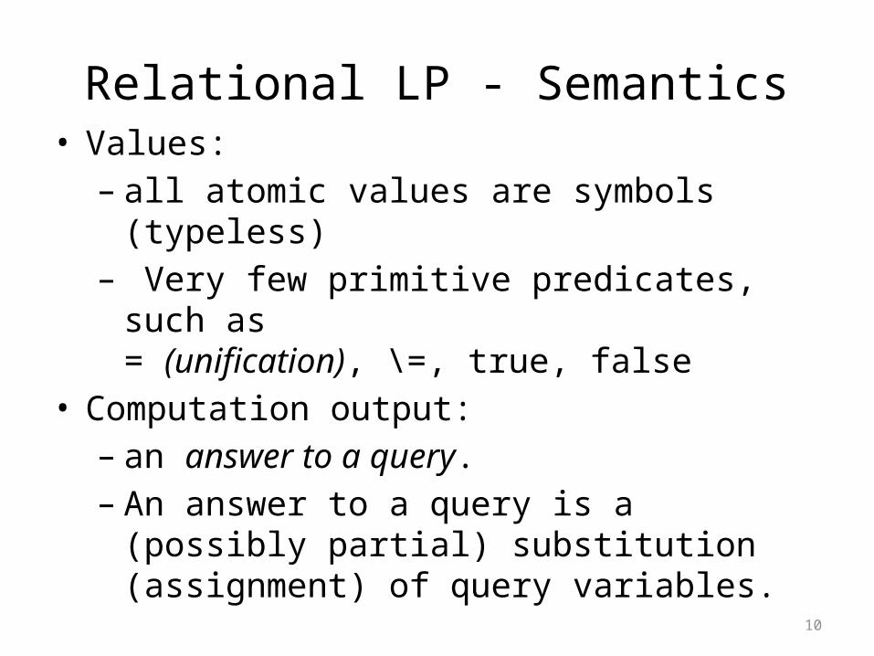
Relational LP - Semantics• Values: – all atomic values are symbols (typeless)– Very few primitive predicates, such as
= (unification), \=, true, false • Computation output: – an answer to a query.– An answer to a query is a (possibly partial)
substitution (assignment) of query variables.
11
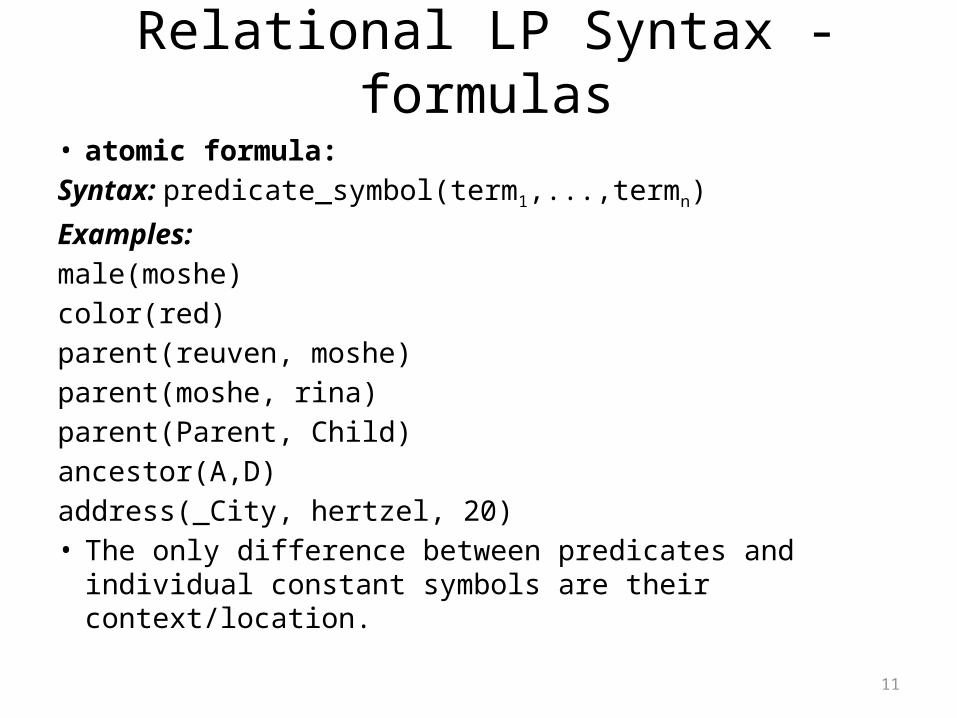
Relational LP Syntax - formulas• atomic formula:Syntax: predicate_symbol(term1,...,termn)
Examples:male(moshe)color(red)parent(reuven, moshe)parent(moshe, rina)parent(Parent, Child)ancestor(A,D)address(_City, hertzel, 20)• The only difference between predicates and individual constant
symbols are their context/location.
12
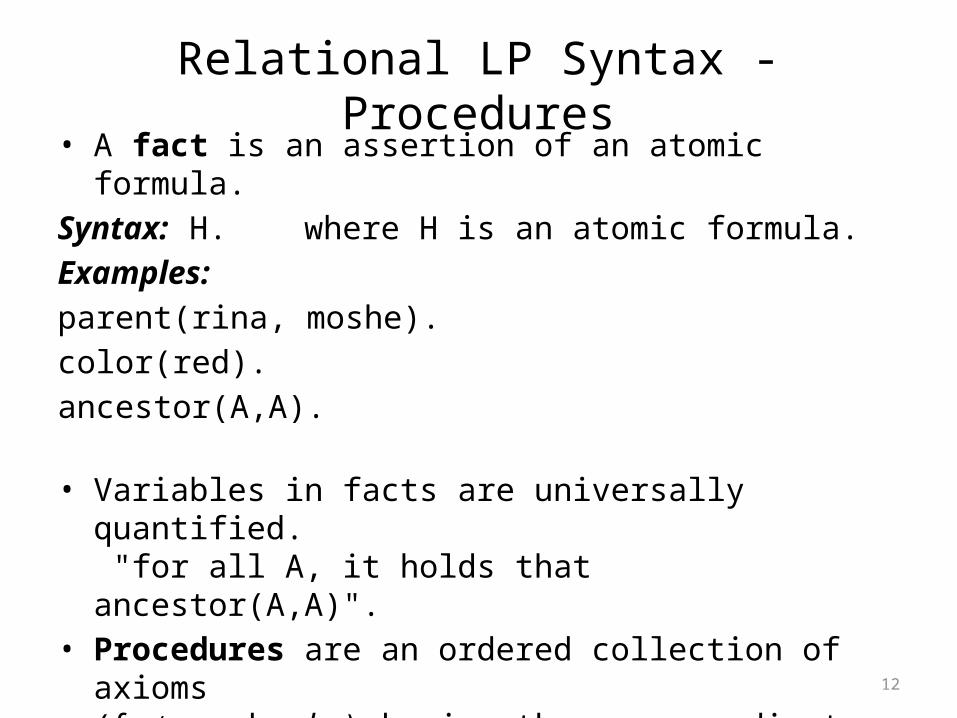
Relational LP Syntax - Procedures• A fact is an assertion of an atomic formula. Syntax: H. where H is an atomic formula.Examples:parent(rina, moshe).color(red).ancestor(A,A).
• Variables in facts are universally quantified. "for all A, it holds that ancestor(A,A)".
• Procedures are an ordered collection of axioms (facts and rules) sharing the same predicate name and arity.
13
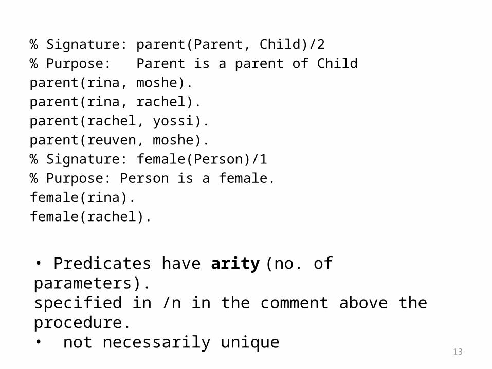
% Signature: parent(Parent, Child)/2% Purpose: Parent is a parent of Childparent(rina, moshe).parent(rina, rachel).parent(rachel, yossi).parent(reuven, moshe).% Signature: female(Person)/1% Purpose: Person is a female.female(rina).female(rachel).
• Predicates have arity (no. of parameters). specified in /n in the comment above the procedure.• not necessarily unique
14
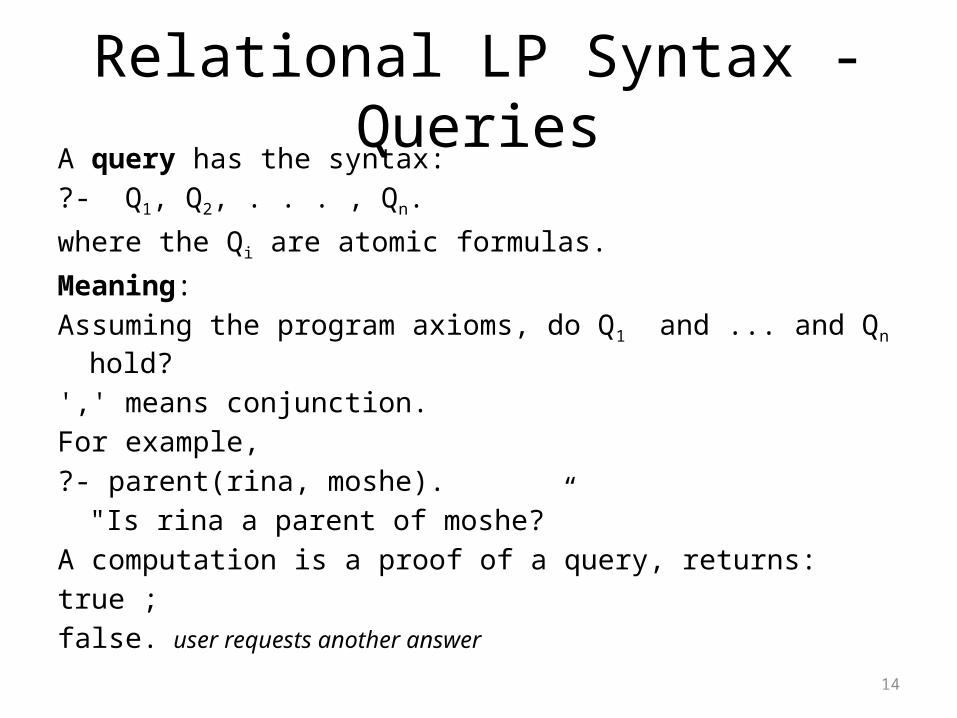
Relational LP Syntax - QueriesA query has the syntax:?- Q1, Q2, . . . , Qn.
where the Qi are atomic formulas.
Meaning: Assuming the program axioms, do Q1 and ... and Qn hold?
',' means conjunction.For example, ?- parent(rina, moshe).
"Is rina a parent of moshe?”A computation is a proof of a query, returns:true ;false. user requests another answer
15
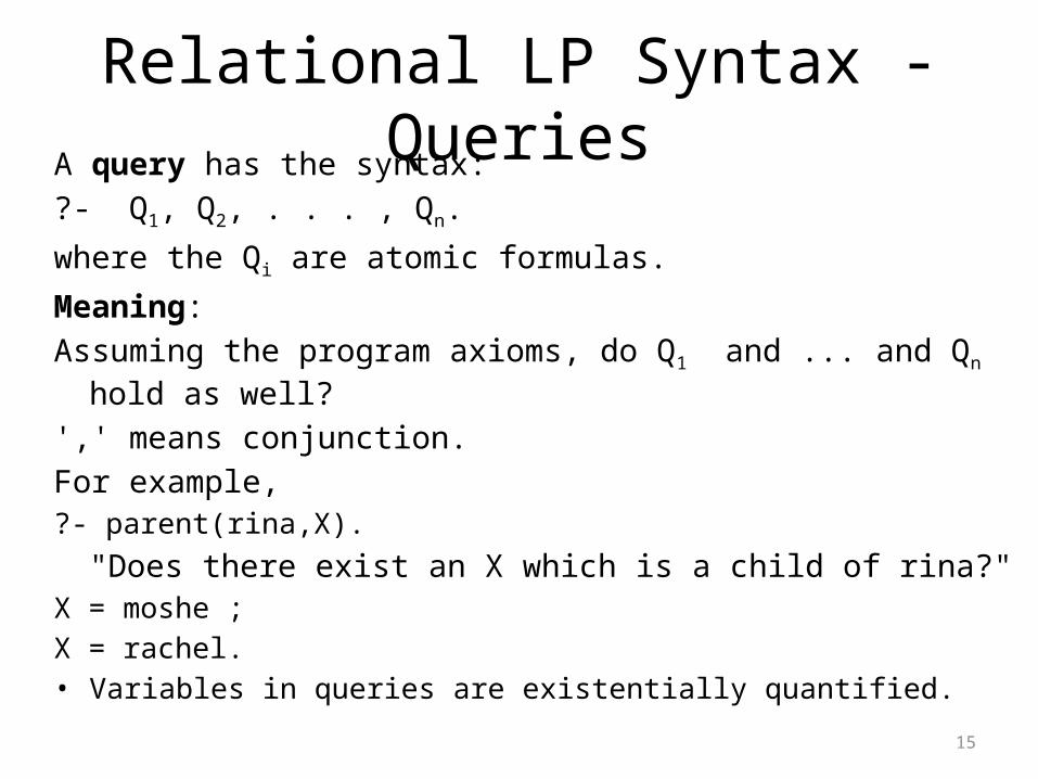
Relational LP Syntax - QueriesA query has the syntax:?- Q1, Q2, . . . , Qn.
where the Qi are atomic formulas.
Meaning: Assuming the program axioms, do Q1 and ... and Qn hold as well?
',' means conjunction.For example, ?- parent(rina,X).
"Does there exist an X which is a child of rina?"X = moshe ;X = rachel. • Variables in queries are existentially quantified.
16
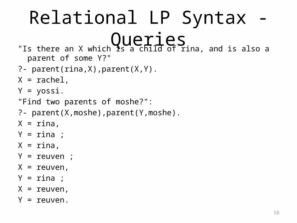
Relational LP Syntax - Queries"Is there an X which is a child of rina, and is also a parent of some Y?"?- parent(rina,X),parent(X,Y).X = rachel,Y = yossi."Find two parents of moshe?":?- parent(X,moshe),parent(Y,moshe).X = rina,Y = rina ;X = rina,Y = reuven ;X = reuven,Y = rina ;X = reuven,Y = reuven.
17
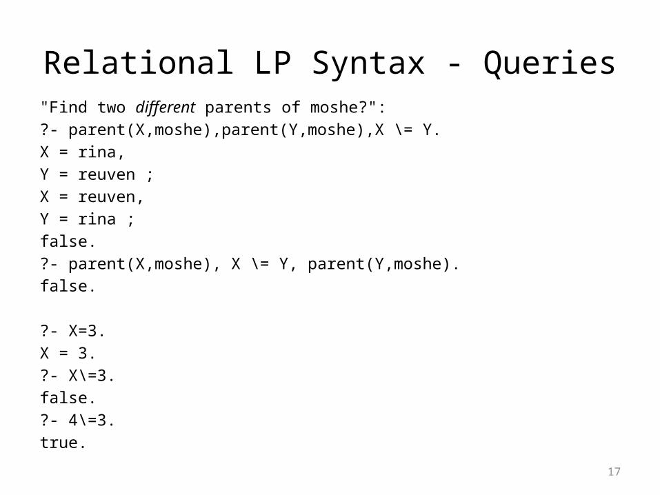
Relational LP Syntax - Queries"Find two different parents of moshe?":?- parent(X,moshe),parent(Y,moshe),X \= Y.X = rina,Y = reuven ;X = reuven,Y = rina ;false.?- parent(X,moshe), X \= Y, parent(Y,moshe).false.
?- X=3.X = 3.?- X\=3.false.?- 4\=3.true.
18
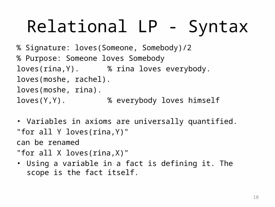
Relational LP - Syntax% Signature: loves(Someone, Somebody)/2% Purpose: Someone loves Somebodyloves(rina,Y). % rina loves everybody.loves(moshe, rachel).loves(moshe, rina).loves(Y,Y). % everybody loves himself
• Variables in axioms are universally quantified."for all Y loves(rina,Y)"can be renamed "for all X loves(rina,X)"• Using a variable in a fact is defining it. The scope is the fact itself.
19
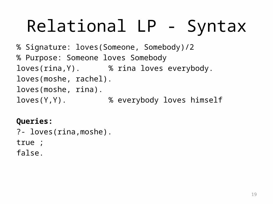
Relational LP - Syntax% Signature: loves(Someone, Somebody)/2% Purpose: Someone loves Somebodyloves(rina,Y). % rina loves everybody.loves(moshe, rachel).loves(moshe, rina).loves(Y,Y). % everybody loves himself
Queries:?- loves(rina,moshe).true ;false.
20
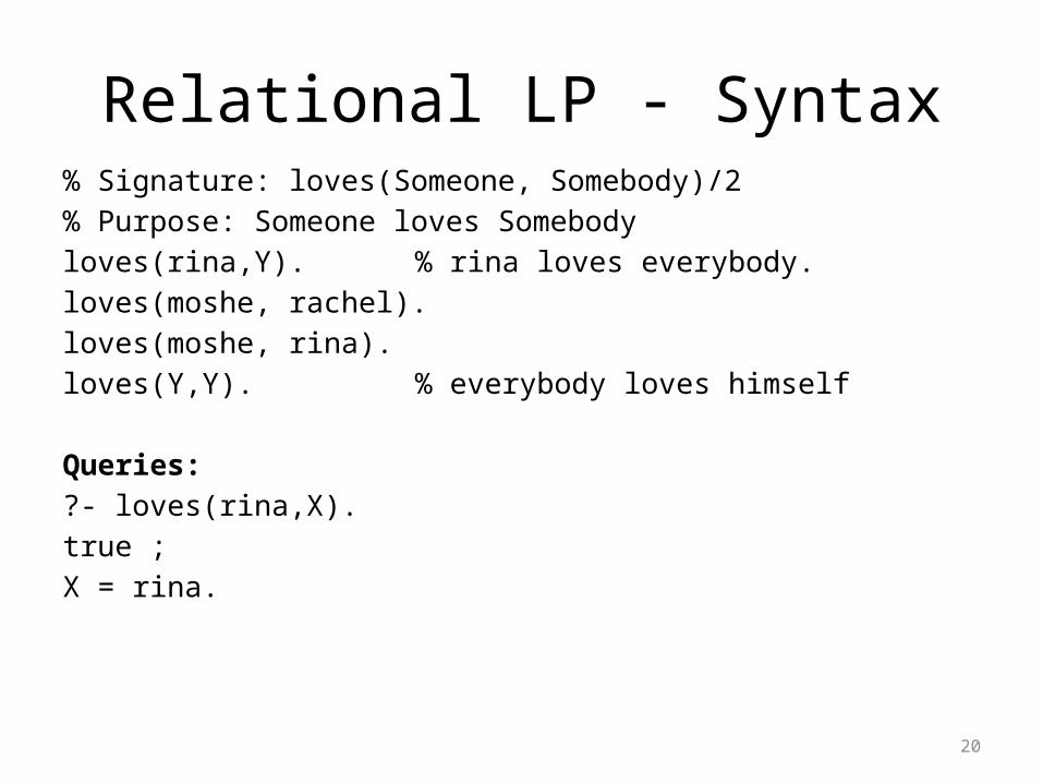
Relational LP - Syntax% Signature: loves(Someone, Somebody)/2% Purpose: Someone loves Somebodyloves(rina,Y). % rina loves everybody.loves(moshe, rachel).loves(moshe, rina).loves(Y,Y). % everybody loves himself
Queries:?- loves(rina,X).true ;X = rina.
21
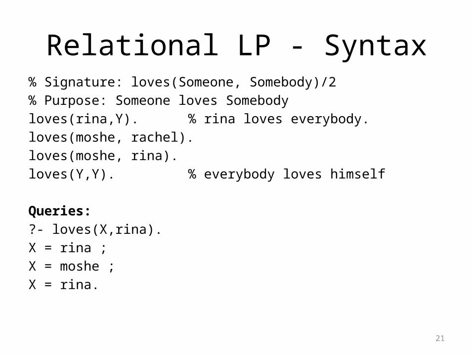
Relational LP - Syntax% Signature: loves(Someone, Somebody)/2% Purpose: Someone loves Somebodyloves(rina,Y). % rina loves everybody.loves(moshe, rachel).loves(moshe, rina).loves(Y,Y). % everybody loves himself
Queries:?- loves(X,rina).X = rina ;X = moshe ;X = rina.
22
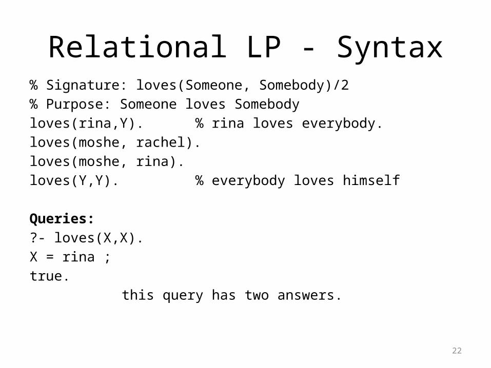
Relational LP - Syntax% Signature: loves(Someone, Somebody)/2% Purpose: Someone loves Somebodyloves(rina,Y). % rina loves everybody.loves(moshe, rachel).loves(moshe, rina).loves(Y,Y). % everybody loves himself
Queries:?- loves(X,X).X = rina ;true.
this query has two answers.
23
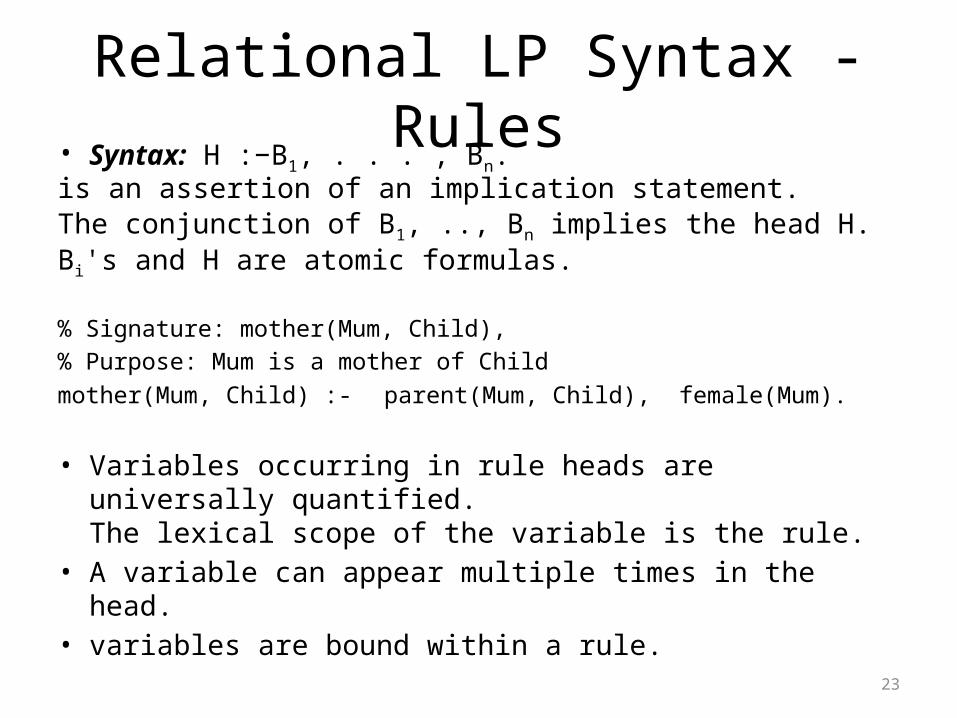
Relational LP Syntax - Rules• Syntax: H :−B1, . . . , Bn.is an assertion of an implication statement. The conjunction of B1, .., Bn implies the head H. Bi's and H are atomic formulas.
% Signature: mother(Mum, Child),% Purpose: Mum is a mother of Child
mother(Mum, Child) :- parent(Mum, Child), female(Mum).
• Variables occurring in rule heads are universally quantified. The lexical scope of the variable is the rule.
• A variable can appear multiple times in the head.• variables are bound within a rule.
24
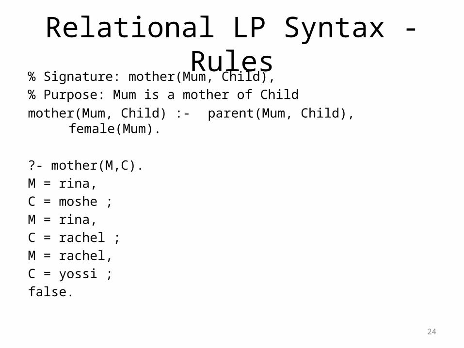
Relational LP Syntax - Rules% Signature: mother(Mum, Child),% Purpose: Mum is a mother of Child
mother(Mum, Child) :- parent(Mum, Child), female(Mum).
?- mother(M,C).M = rina,C = moshe ;M = rina,C = rachel ;M = rachel,C = yossi ;false.
25
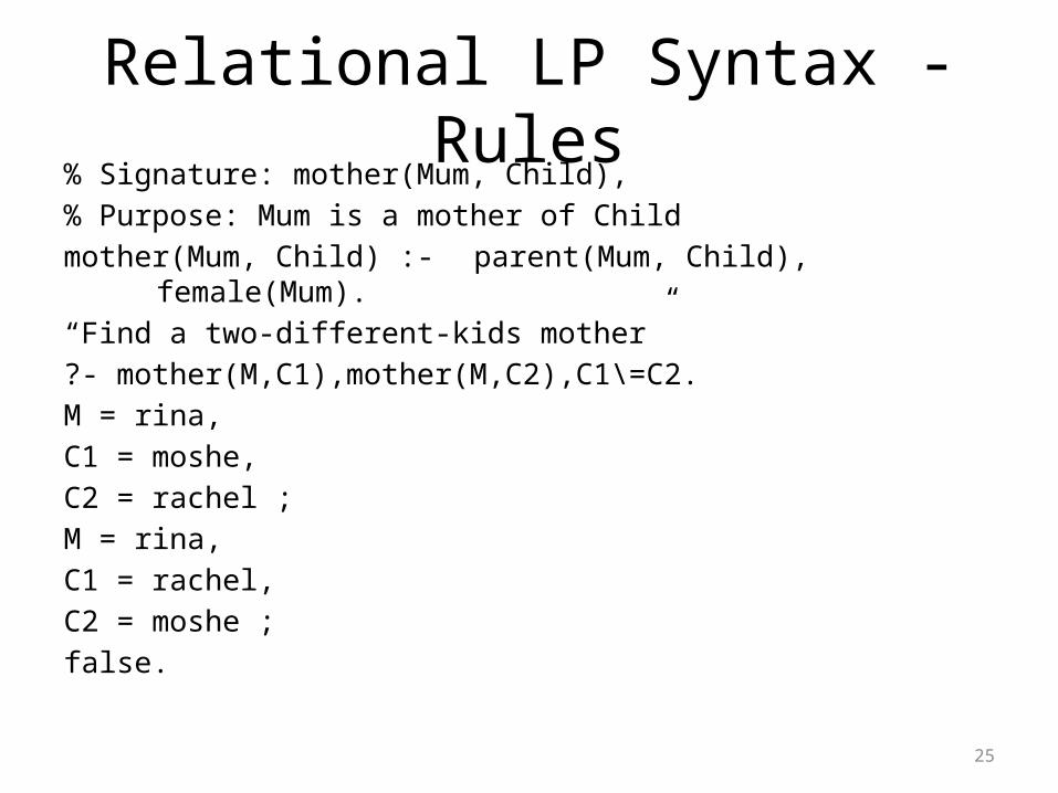
Relational LP Syntax - Rules% Signature: mother(Mum, Child),% Purpose: Mum is a mother of Childmother(Mum, Child) :- parent(Mum, Child),
female(Mum). “Find a two-different-kids mother”?- mother(M,C1),mother(M,C2),C1\=C2.M = rina,C1 = moshe,C2 = rachel ;M = rina,C1 = rachel,C2 = moshe ;false.
26
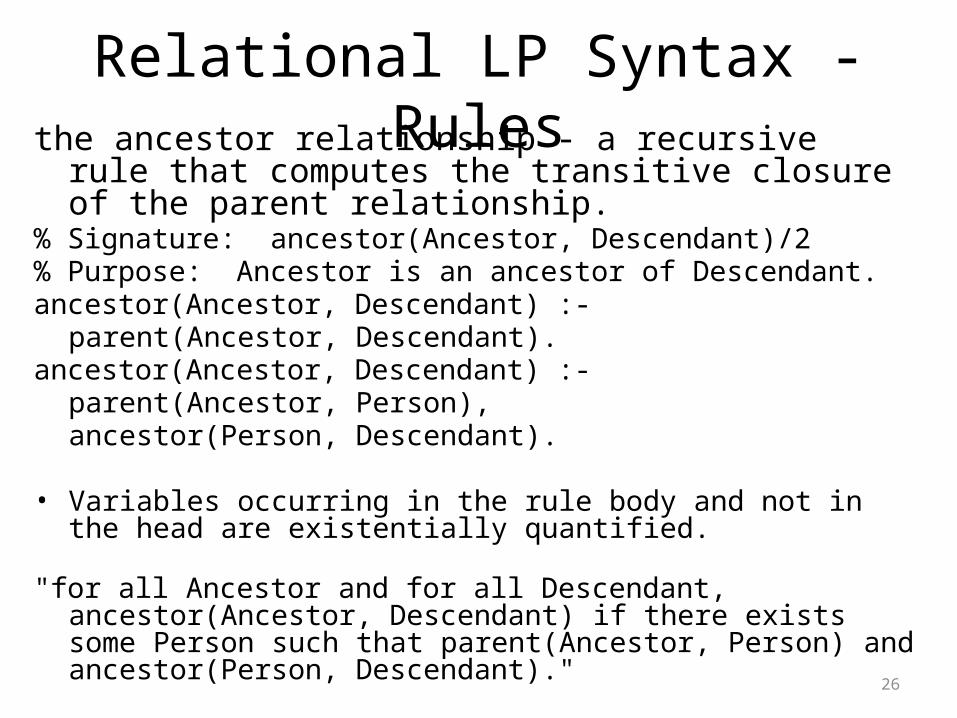
Relational LP Syntax - Rulesthe ancestor relationship - a recursive rule that computes the
transitive closure of the parent relationship.% Signature: ancestor(Ancestor, Descendant)/2% Purpose: Ancestor is an ancestor of Descendant.ancestor(Ancestor, Descendant) :-
parent(Ancestor, Descendant).ancestor(Ancestor, Descendant) :-
parent(Ancestor, Person),ancestor(Person, Descendant).
• Variables occurring in the rule body and not in the head are existentially quantified.
"for all Ancestor and for all Descendant, ancestor(Ancestor, Descendant) if there exists some Person such that parent(Ancestor, Person) and ancestor(Person, Descendant)."
27
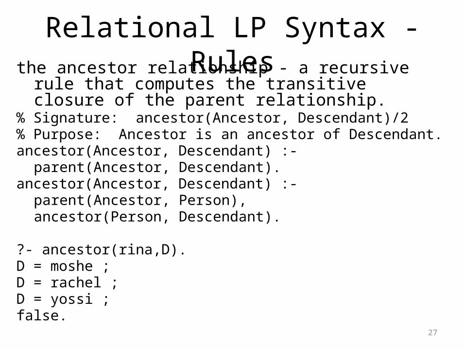
Relational LP Syntax - Rulesthe ancestor relationship - a recursive rule that computes the
transitive closure of the parent relationship.% Signature: ancestor(Ancestor, Descendant)/2% Purpose: Ancestor is an ancestor of Descendant.ancestor(Ancestor, Descendant) :-
parent(Ancestor, Descendant).ancestor(Ancestor, Descendant) :-
parent(Ancestor, Person),ancestor(Person, Descendant).
?- ancestor(rina,D).D = moshe ;D = rachel ;D = yossi ;false.
28
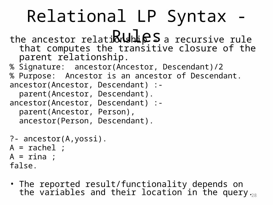
Relational LP Syntax - Rulesthe ancestor relationship - a recursive rule that computes the
transitive closure of the parent relationship.% Signature: ancestor(Ancestor, Descendant)/2% Purpose: Ancestor is an ancestor of Descendant.ancestor(Ancestor, Descendant) :-
parent(Ancestor, Descendant).ancestor(Ancestor, Descendant) :-
parent(Ancestor, Person),ancestor(Person, Descendant).
?- ancestor(A,yossi).A = rachel ;A = rina ;false.
• The reported result/functionality depends on the variables and their location in the query.
29
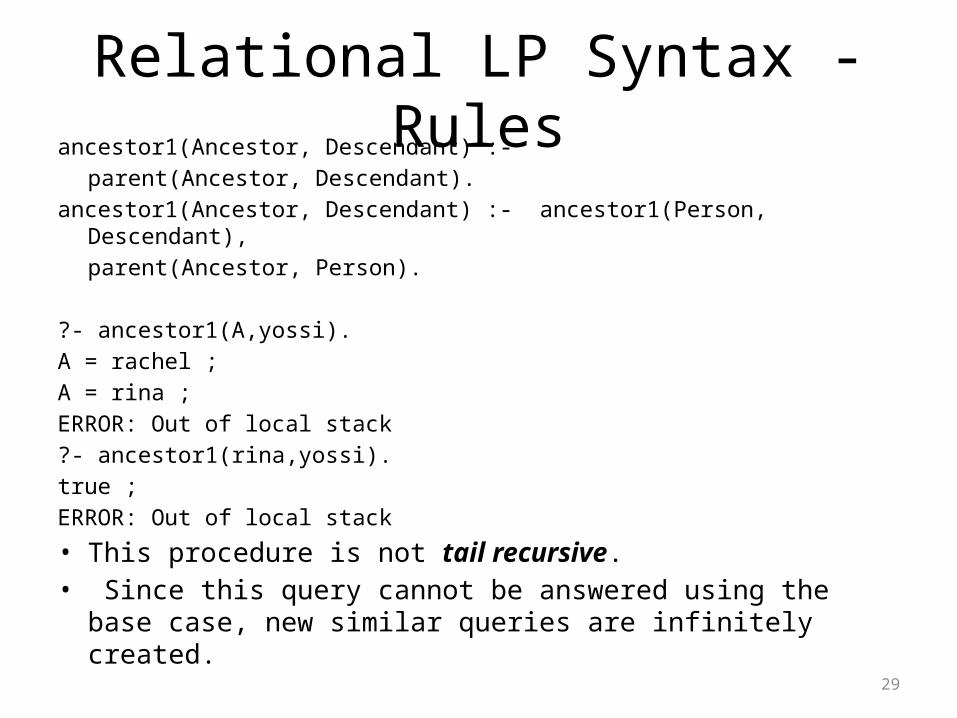
Relational LP Syntax - Rulesancestor1(Ancestor, Descendant) :-
parent(Ancestor, Descendant).ancestor1(Ancestor, Descendant) :- ancestor1(Person,
Descendant),parent(Ancestor, Person).
?- ancestor1(A,yossi).A = rachel ;A = rina ;ERROR: Out of local stack?- ancestor1(rina,yossi).true ;ERROR: Out of local stack
• This procedure is not tail recursive.• Since this query cannot be answered using the base case, new
similar queries are infinitely created.
30
Note
Facts can be considered as rules with an empty body.
For example, parent(rina, moshe).parent(rina, moshe):- true.have equivalent meaning.
true - is the zero-arity predicate.
31
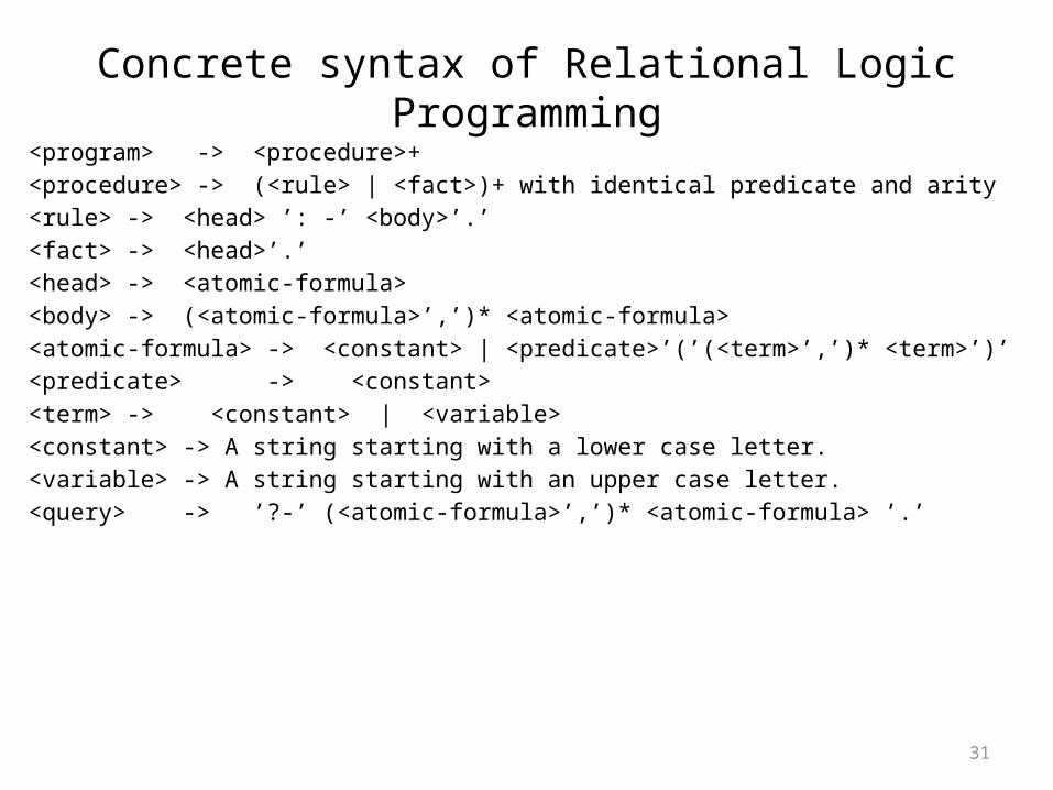
Concrete syntax of Relational Logic Programming<program> -> <procedure>+<procedure> -> (<rule> | <fact>)+ with identical predicate and arity<rule> -> <head> ’: -’ <body>’.’<fact> -> <head>’.’<head> -> <atomic-formula><body> -> (<atomic-formula>’,’)* <atomic-formula><atomic-formula> -> <constant> | <predicate>’(’(<term>’,’)* <term>’)’<predicate> -> <constant><term> -> <constant> | <variable><constant> -> A string starting with a lower case letter.<variable> -> A string starting with an upper case letter.<query> -> ’?-’ (<atomic-formula>’,’)* <atomic-formula> ’.’
32
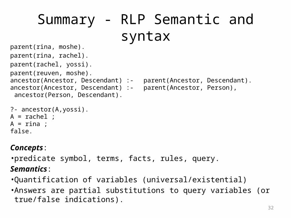
Summary - RLP Semantic and syntaxparent(rina, moshe).parent(rina, rachel).parent(rachel, yossi).parent(reuven, moshe).ancestor(Ancestor, Descendant) :- parent(Ancestor, Descendant).ancestor(Ancestor, Descendant) :- parent(Ancestor, Person),
ancestor(Person, Descendant).
?- ancestor(A,yossi).A = rachel ;A = rina ;false.
Concepts: • predicate symbol, terms, facts, rules, query.Semantics: • Quantification of variables (universal/existential)• Answers are partial substitutions to query variables (or true/false indications).
33
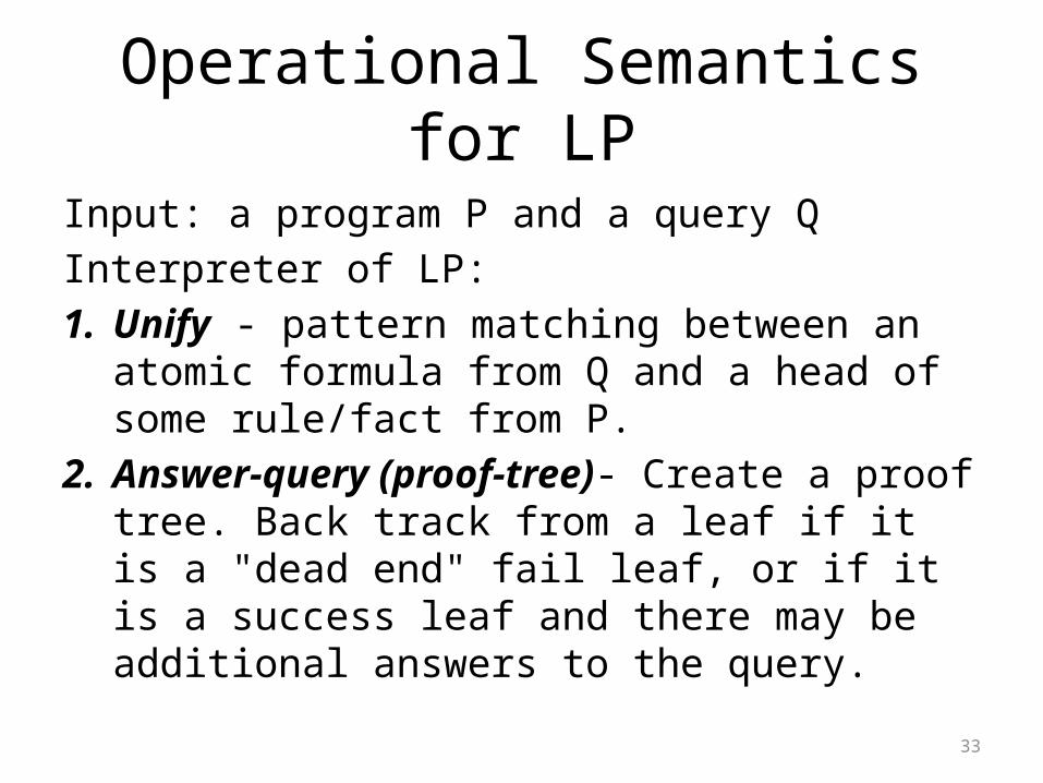
Operational Semantics for LP
Input: a program P and a query QInterpreter of LP:1. Unify - pattern matching between an atomic
formula from Q and a head of some rule/fact from P.
2. Answer-query (proof-tree)- Create a proof tree. Back track from a leaf if it is a "dead end" fail leaf, or if it is a success leaf and there may be additional answers to the query.
34
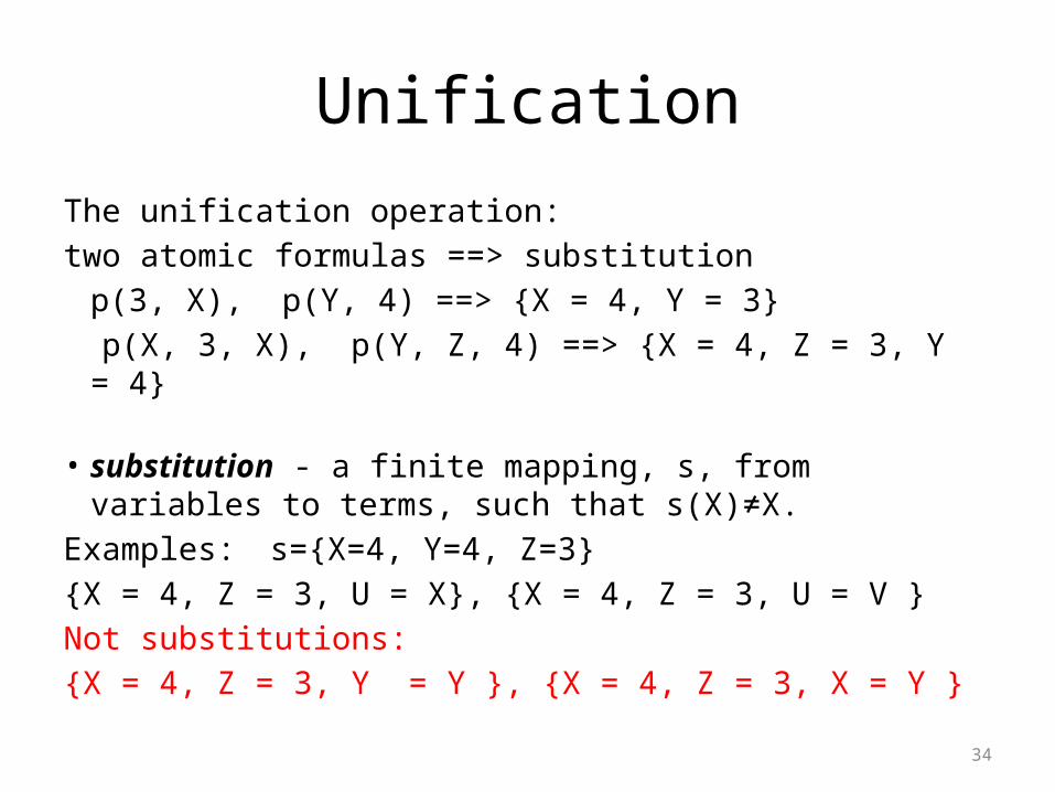
Unification
The unification operation:two atomic formulas ==> substitution
p(3, X), p(Y, 4) ==> {X = 4, Y = 3} p(X, 3, X), p(Y, Z, 4) ==> {X = 4, Z = 3, Y = 4}
• substitution - a finite mapping, s, from variables to terms, such that s(X)≠X.
Examples: s={X=4, Y=4, Z=3}{X = 4, Z = 3, U = X}, {X = 4, Z = 3, U = V }Not substitutions: {X = 4, Z = 3, Y = Y }, {X = 4, Z = 3, X = Y }
35
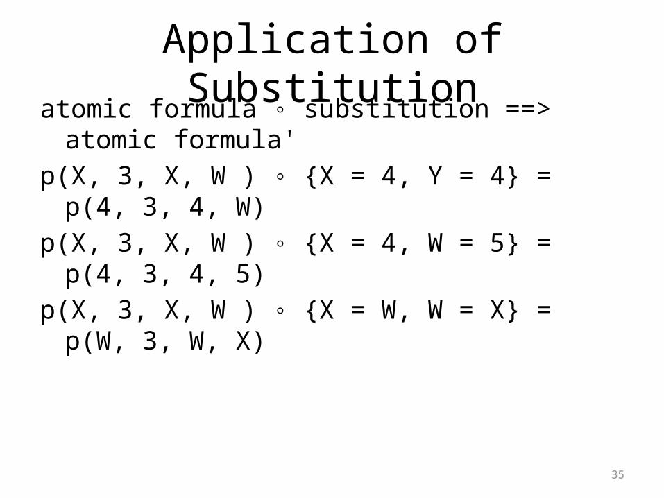
Application of Substitutionatomic formula ◦ substitution ==> atomic formula'p(X, 3, X, W ) ◦ {X = 4, Y = 4} = p(4, 3, 4, W)
p(X, 3, X, W ) ◦ {X = 4, W = 5} = p(4, 3, 4, 5)
p(X, 3, X, W ) ◦ {X = W, W = X} = p(W, 3, W, X)
36
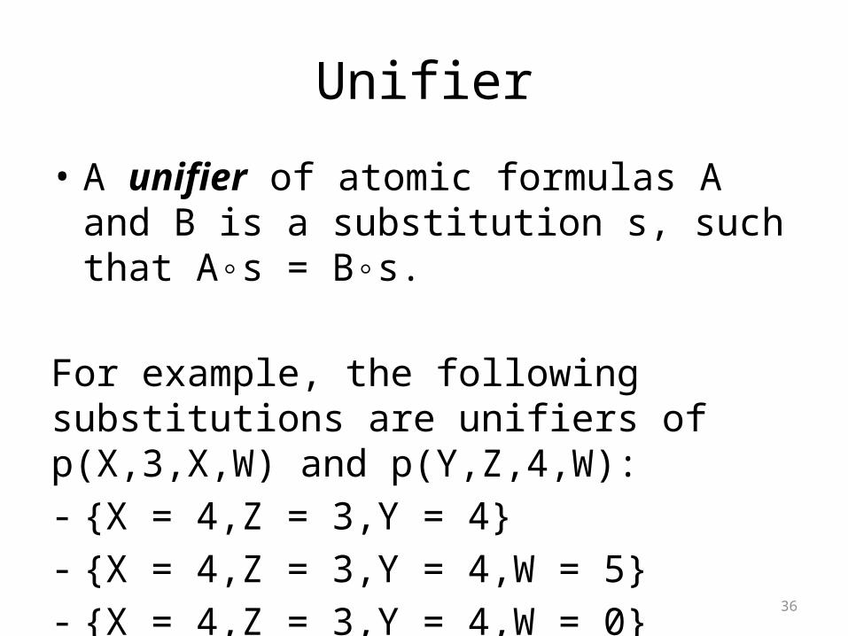
Unifier
• A unifier of atomic formulas A and B is a substitution s, such that A◦s = B◦s.
For example, the following substitutions are unifiers of p(X,3,X,W) and p(Y,Z,4,W):- {X = 4,Z = 3,Y = 4}- {X = 4,Z = 3,Y = 4,W = 5}- {X = 4,Z = 3,Y = 4,W = 0}
37
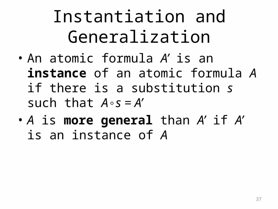
Instantiation and Generalization
• An atomic formula A’ is an instance of an atomic formula A if there is a substitution s such that A◦s = A’
• A is more general than A’ if A’ is an instance of A
38
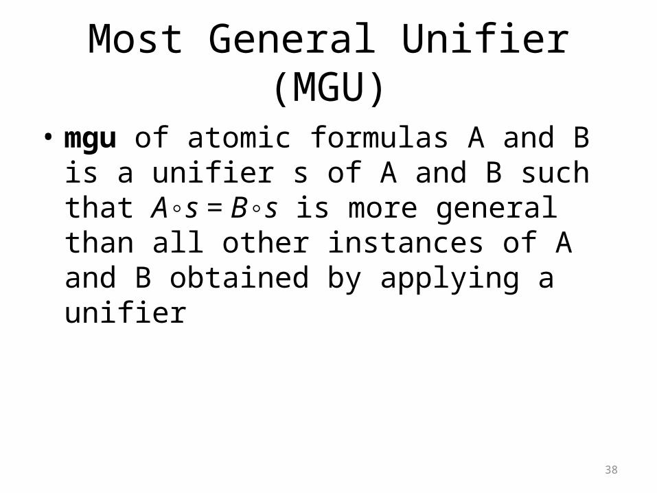
Most General Unifier (MGU)
• mgu of atomic formulas A and B is a unifier s of A and B such that A◦s = B◦s is more general than all other instances of A and B obtained by applying a unifier
39
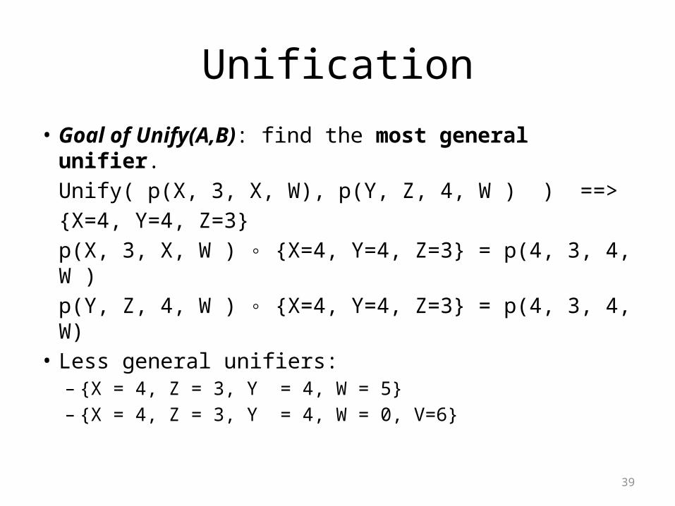
Unification
• Goal of Unify(A,B): find the most general unifier.Unify( p(X, 3, X, W), p(Y, Z, 4, W ) ) ==>
{X=4, Y=4, Z=3} p(X, 3, X, W ) ◦ {X=4, Y=4, Z=3} = p(4, 3, 4, W )p(Y, Z, 4, W ) ◦ {X=4, Y=4, Z=3} = p(4, 3, 4, W)
• Less general unifiers:– {X = 4, Z = 3, Y = 4, W = 5}– {X = 4, Z = 3, Y = 4, W = 0, V=6}

40
Combination of substitutions
s ◦ s'1. s' is applied to the terms of s2. A variable X for which s(X) is defined, is removed from the
domain of s'3. The modified s' is added to s.4. Identity bindings are removed.
{X = Y, Z = 3, U = V } ◦ {Y = 4, W = 5, V = U, Z = X} = {X = 4, Z = 3, Y = 4, W = 5, V = U}.
41
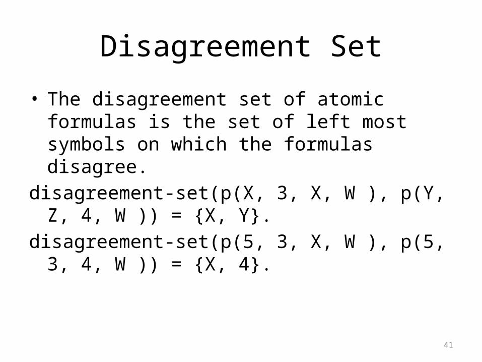
Disagreement Set
• The disagreement set of atomic formulas is the set of left most symbols on which the formulas disagree.
disagreement-set(p(X, 3, X, W ), p(Y, Z, 4, W )) = {X, Y}.disagreement-set(p(5, 3, X, W ), p(5, 3, 4, W )) = {X, 4}.
42
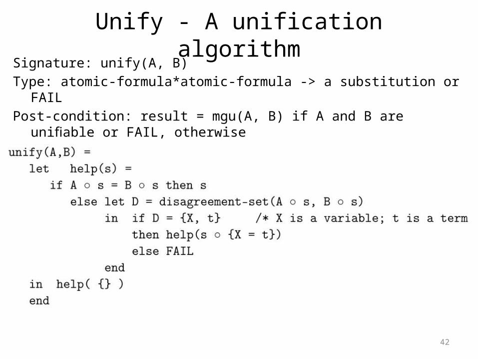
Unify - A unification algorithmSignature: unify(A, B)Type: atomic-formula*atomic-formula -> a substitution or FAILPost-condition: result = mgu(A, B) if A and B are unifiable or FAIL, otherwise
43
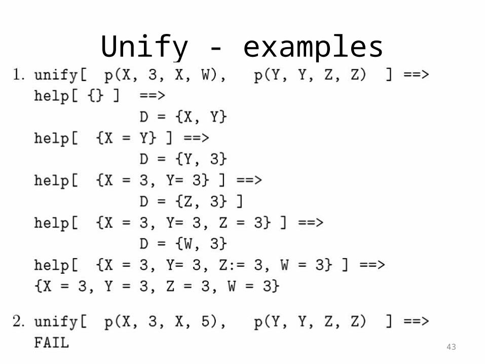
Unify - examples
44
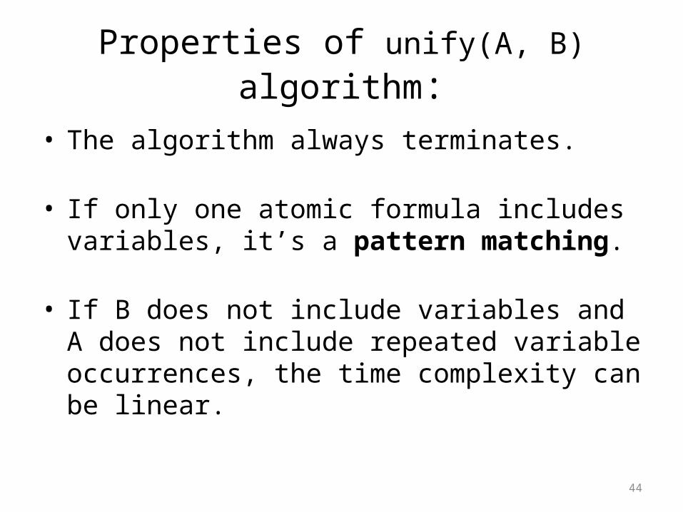
Properties of unify(A, B) algorithm:
• The algorithm always terminates.
• If only one atomic formula includes variables, it’s a pattern matching.
• If B does not include variables and A does not include repeated variable occurrences, the time complexity can be linear.
45
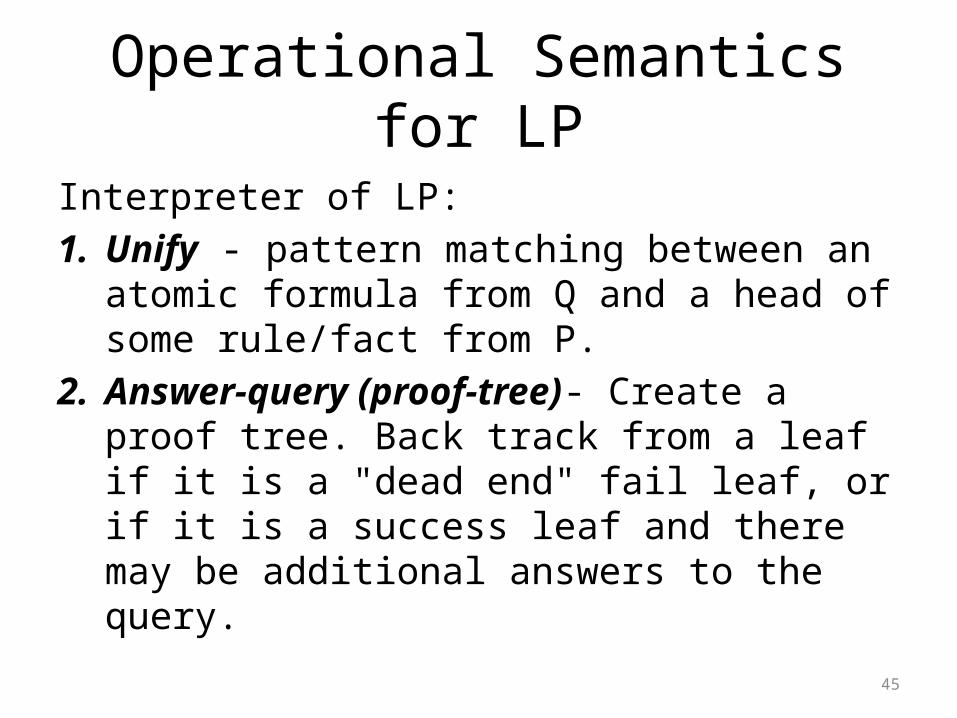
Operational Semantics for LP
Interpreter of LP:1. Unify - pattern matching between an atomic
formula from Q and a head of some rule/fact from P.
2. Answer-query (proof-tree)- Create a proof tree. Back track from a leaf if it is a "dead end" fail leaf, or if it is a success leaf and there may be additional answers to the query.
46
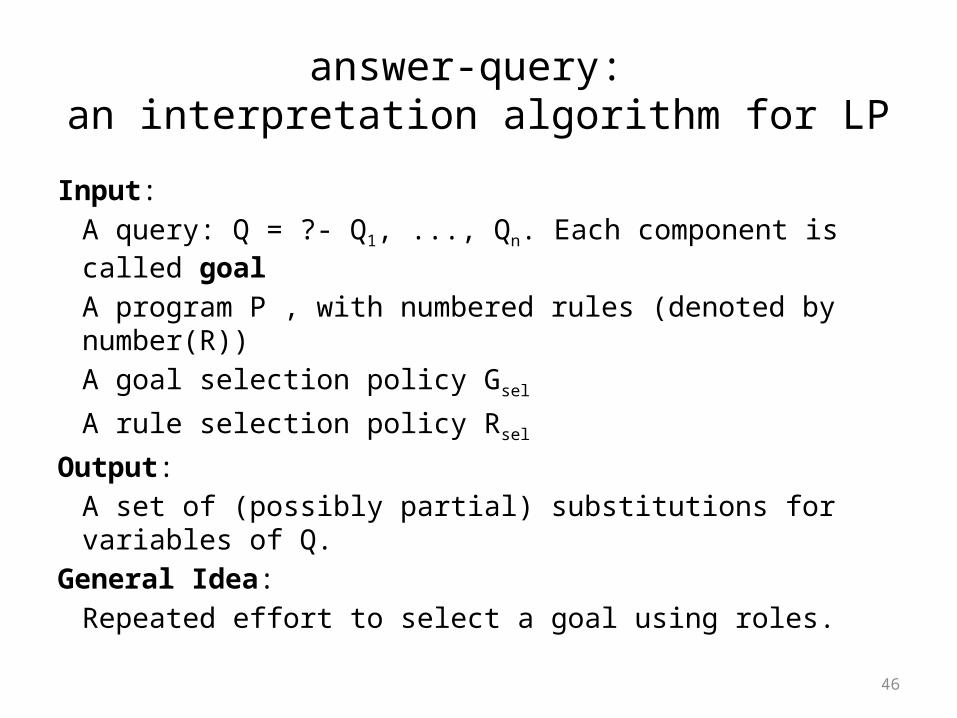
answer-query: an interpretation algorithm for LP
Input:A query: Q = ?- Q1, ..., Qn. Each component is called goal
A program P , with numbered rules (denoted by number(R))A goal selection policy Gsel
A rule selection policy Rsel
Output: A set of (possibly partial) substitutions for variables of Q.
General Idea:Repeated effort to select a goal using roles.
47
answer-query
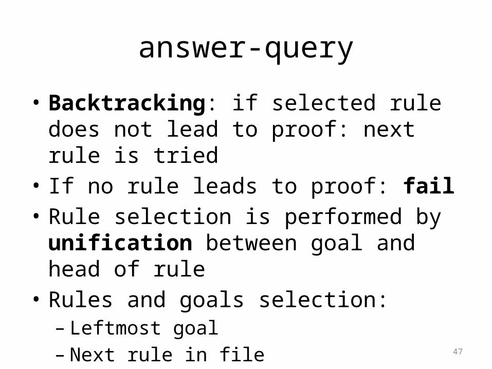
• Backtracking: if selected rule does not lead to proof: next rule is tried
• If no rule leads to proof: fail• Rule selection is performed by unification
between goal and head of rule• Rules and goals selection:– Leftmost goal– Next rule in file
48
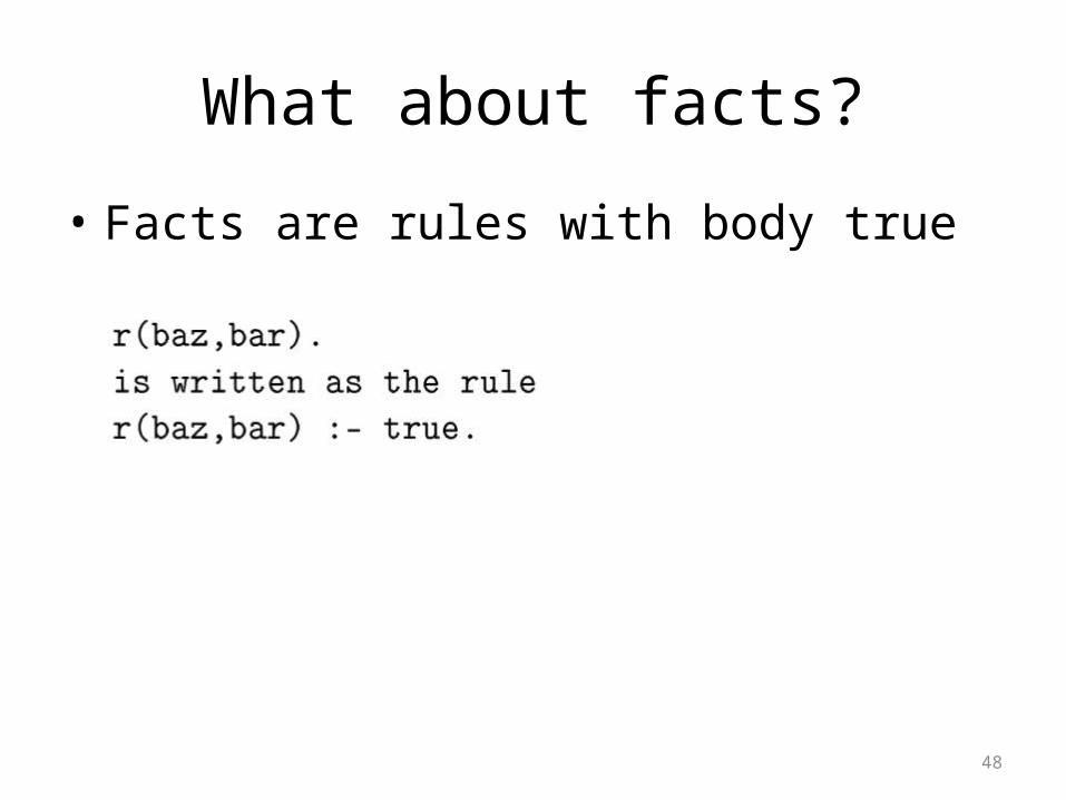
What about facts?
• Facts are rules with body true
49
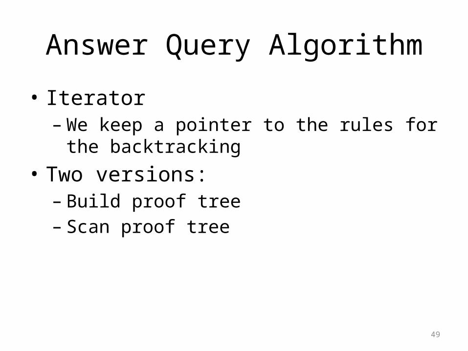
Answer Query Algorithm
• Iterator– We keep a pointer to the rules for the
backtracking• Two versions:– Build proof tree– Scan proof tree

50
Proof Tree
Tree with labeled nodes and edges• Nodes labeled by queries and marked goals• Edges labeled by substitutions and rule
numbers• Root node is input query• Children on node are all successful rules for
the goal
51
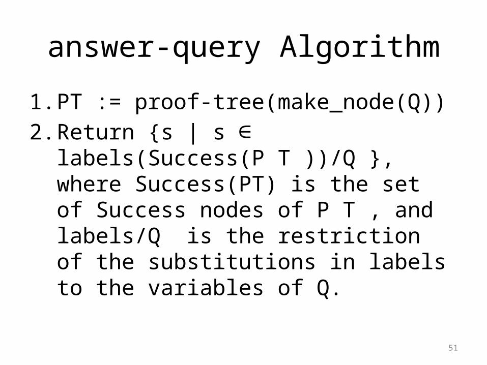
answer-query Algorithm
1. PT := proof-tree(make_node(Q))2. Return {s | s labels(Success(P T ))/Q }, ∈
where Success(PT) is the set of Success nodes of P T , and labels/Q is the restriction of the substitutions in labels to the variables of Q.
52
Possible Answers
• Empty set (fail of query with variables)• Empty set (success for grounded query)• Answer
53
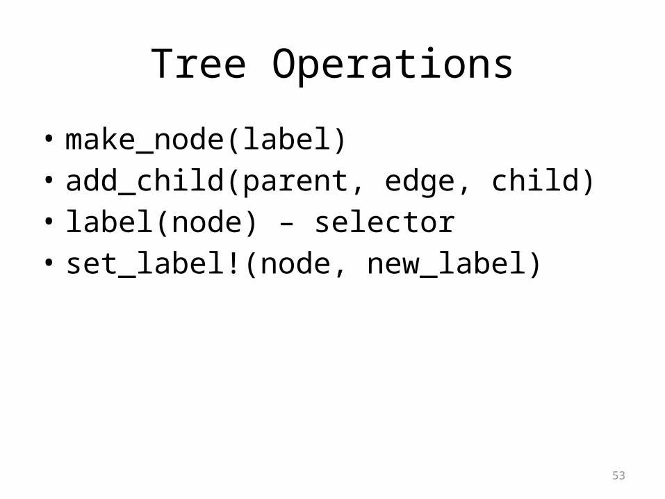
Tree Operations
• make_node(label)• add_child(parent, edge, child)• label(node) – selector• set_label!(node, new_label)
54
55
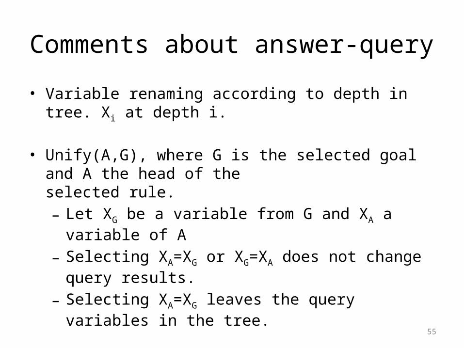
Comments about answer-query
• Variable renaming according to depth in tree. Xi at depth i.
• Unify(A,G), where G is the selected goal and A the head of the
selected rule. – Let XG be a variable from G and XA a variable of A
– Selecting XA=XG or XG=XA does not change query results.
– Selecting XA=XG leaves the query variables in the tree.
• The goal and rule selection decisions can affect the performance of the interpreter.
56
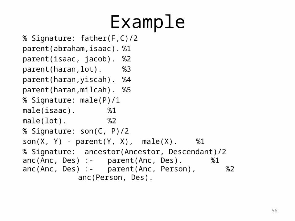
Example% Signature: father(F,C)/2parent(abraham,isaac). %1parent(isaac, jacob). %2parent(haran,lot). %3parent(haran,yiscah). %4parent(haran,milcah). %5% Signature: male(P)/1male(isaac). %1male(lot). %2% Signature: son(C, P)/2son(X, Y) - parent(Y, X), male(X). %1% Signature: ancestor(Ancestor, Descendant)/2anc(Anc, Des) :- parent(Anc, Des). %1anc(Anc, Des) :- parent(Anc, Person),
%2anc(Person, Des).
57
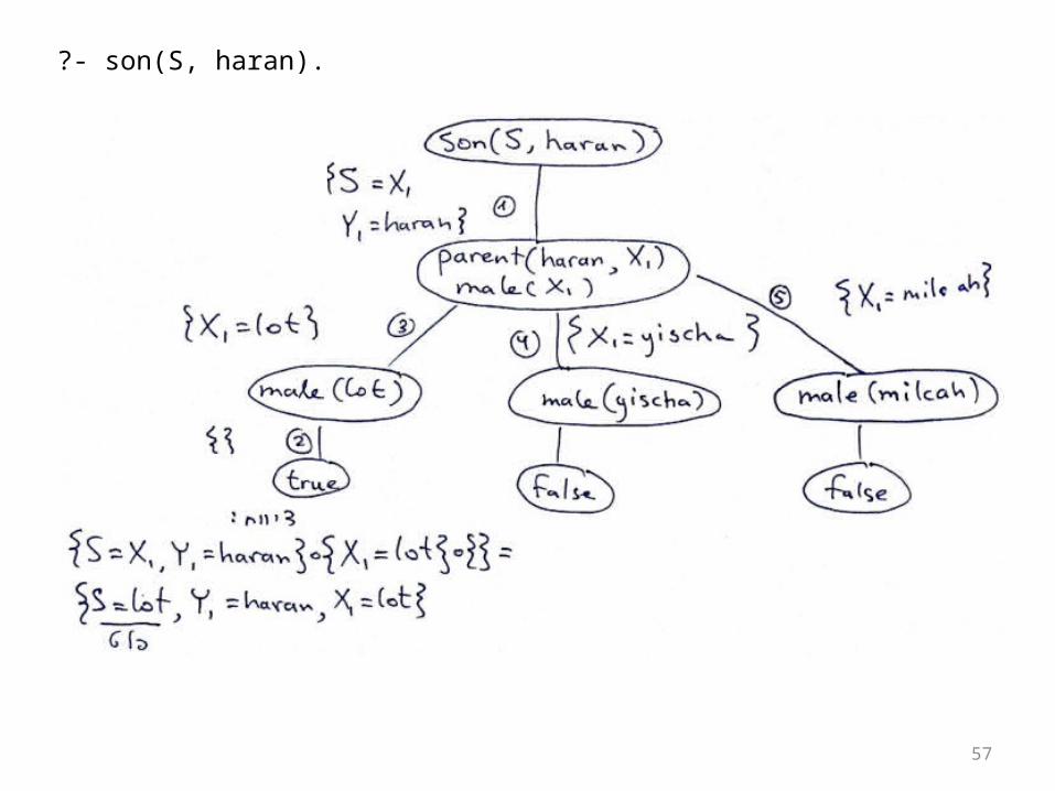
?- son(S, haran).
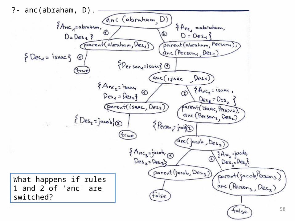
?- anc(abraham, D).
58
What happens if rules 1 and 2 of 'anc' are switched?
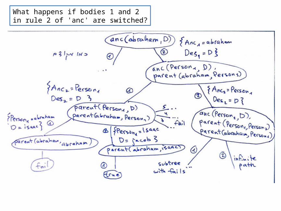
What happens if bodies 1 and 2 in rule 2 of 'anc' are switched?
60
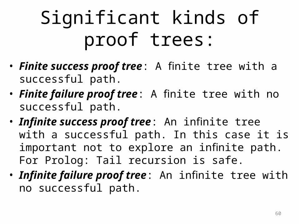
Significant kinds of proof trees: • Finite success proof tree: A finite tree with a successful path.• Finite failure proof tree: A finite tree with no successful path.• Infinite success proof tree: An infinite tree with a successful
path. In this case it is important not to explore an infinite path. For Prolog: Tail recursion is safe.
• Infinite failure proof tree: An infinite tree with no successful path.
61
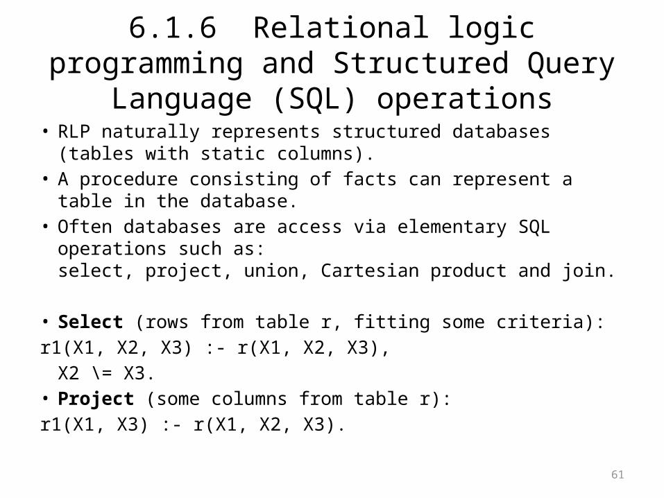
6.1.6 Relational logic programming and Structured Query Language (SQL) operations
• RLP naturally represents structured databases (tables with static columns).
• A procedure consisting of facts can represent a table in the database.
• Often databases are access via elementary SQL operations such as: select, project, union, Cartesian product and join.
• Select (rows from table r, fitting some criteria):r1(X1, X2, X3) :- r(X1, X2, X3),
X2 \= X3.• Project (some columns from table r):r1(X1, X3) :- r(X1, X2, X3).
62
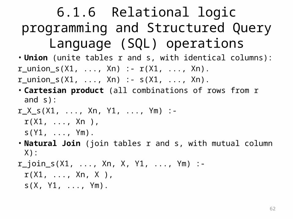
6.1.6 Relational logic programming and Structured Query Language (SQL) operations
• Union (unite tables r and s, with identical columns):r_union_s(X1, ..., Xn) :- r(X1, ..., Xn).r_union_s(X1, ..., Xn) :- s(X1, ..., Xn).• Cartesian product (all combinations of rows from r and s):r_X_s(X1, ..., Xn, Y1, ..., Ym) :-
r(X1, ..., Xn ), s(Y1, ..., Ym).
• Natural Join (join tables r and s, with mutual column X):r_join_s(X1, ..., Xn, X, Y1, ..., Ym) :-
r(X1, ..., Xn, X ), s(X, Y1, ..., Ym).
63
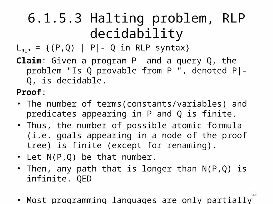
6.1.5.3 Halting problem, RLP decidabilityLRLP = {(P,Q) | P|- Q in RLP syntax}
Claim: Given a program P and a query Q, the problem "Is Q provable from P ", denoted P|- Q, is decidable.
Proof: • The number of terms(constants/variables) and predicates appearing
in P and Q is finite. • Thus, the number of possible atomic formula (i.e. goals appearing in
a node of the proof tree) is finite (except for renaming). • Let N(P,Q) be that number. • Then, any path that is longer than N(P,Q) is infinite. QED
• Most programming languages are only partially decidable (recursively enumerable/TM recognizable)

64
Prolog
LP
Logic Programming
Relational LP
typeless atomic terms, type safedecidablemulti-directional
functors, typeless composite terms, type safepartially decidable, multi-directional
arithmetics, uni-directional dynamically typed,not type safe,system predicates (e.g. !)
65
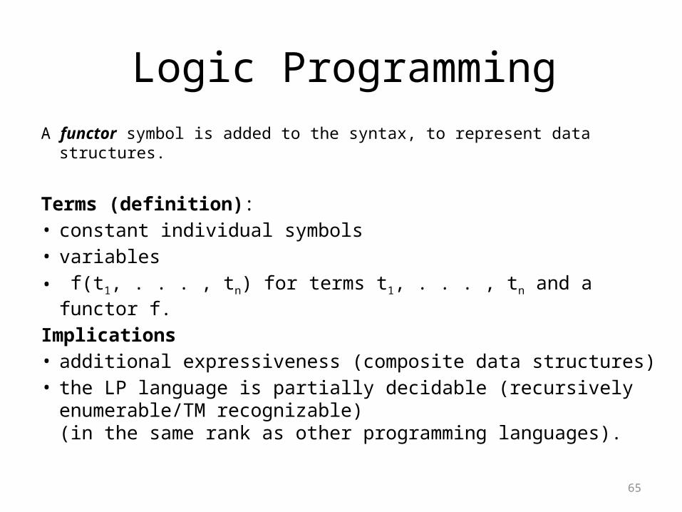
Logic ProgrammingA functor symbol is added to the syntax, to represent data structures.
Terms (definition): • constant individual symbols• variables• f(t1, . . . , tn) for terms t1, . . . , tn and a functor f.
Implications• additional expressiveness (composite data structures)• the LP language is partially decidable (recursively
enumerable/TM recognizable) (in the same rank as other programming languages).
66
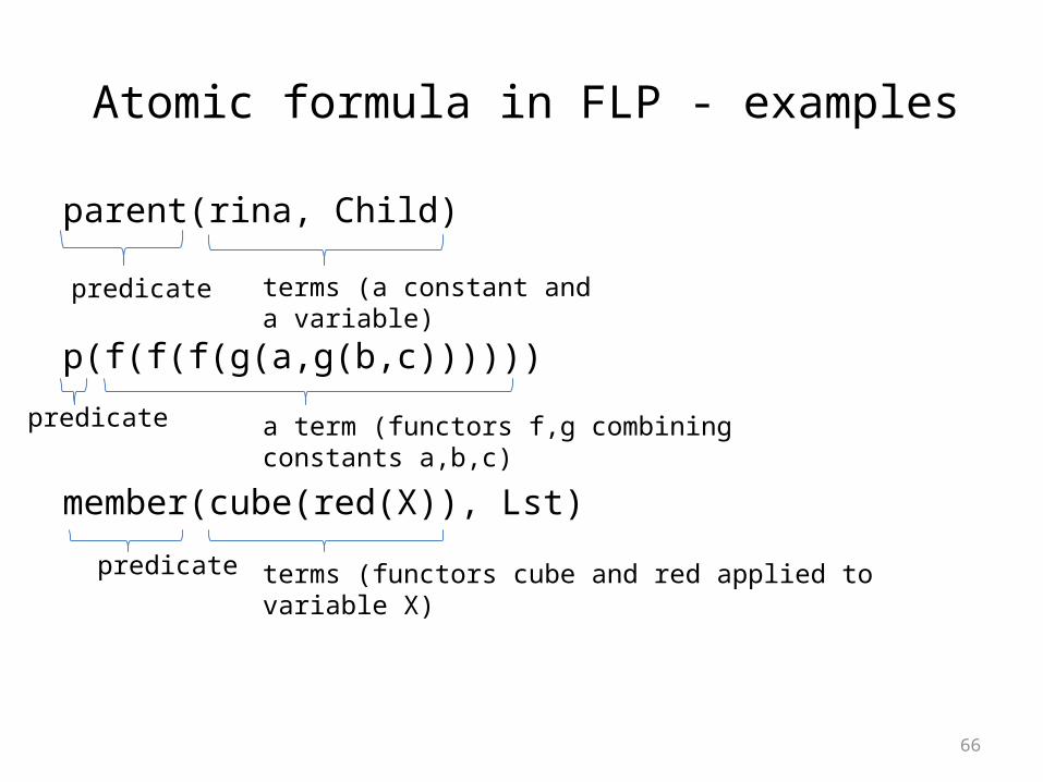
Atomic formula in FLP - examples
parent(rina, Child)
p(f(f(f(g(a,g(b,c))))))
member(cube(red(X)), Lst)
predicate terms (a constant and a variable)
predicate a term (functors f,g combining constants a,b,c)
predicate terms (functors cube and red applied to variable X)
67
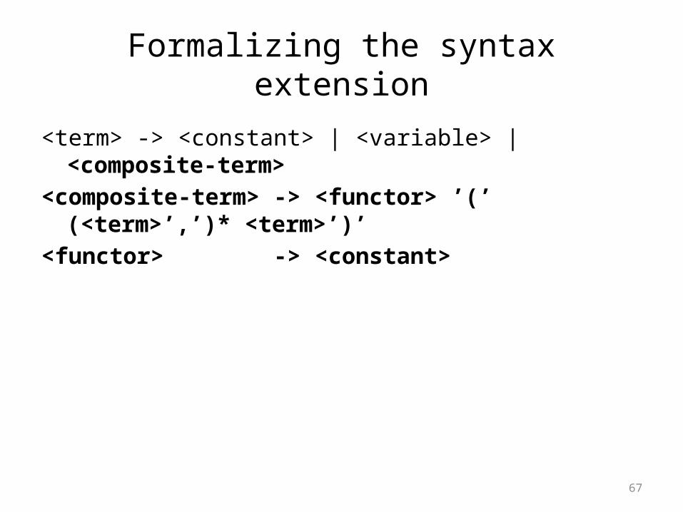
Formalizing the syntax extension
<term> -> <constant> | <variable> | <composite-term><composite-term> -> <functor> ’(’ (<term>’,’)* <term>’)’<functor> -> <constant>

68
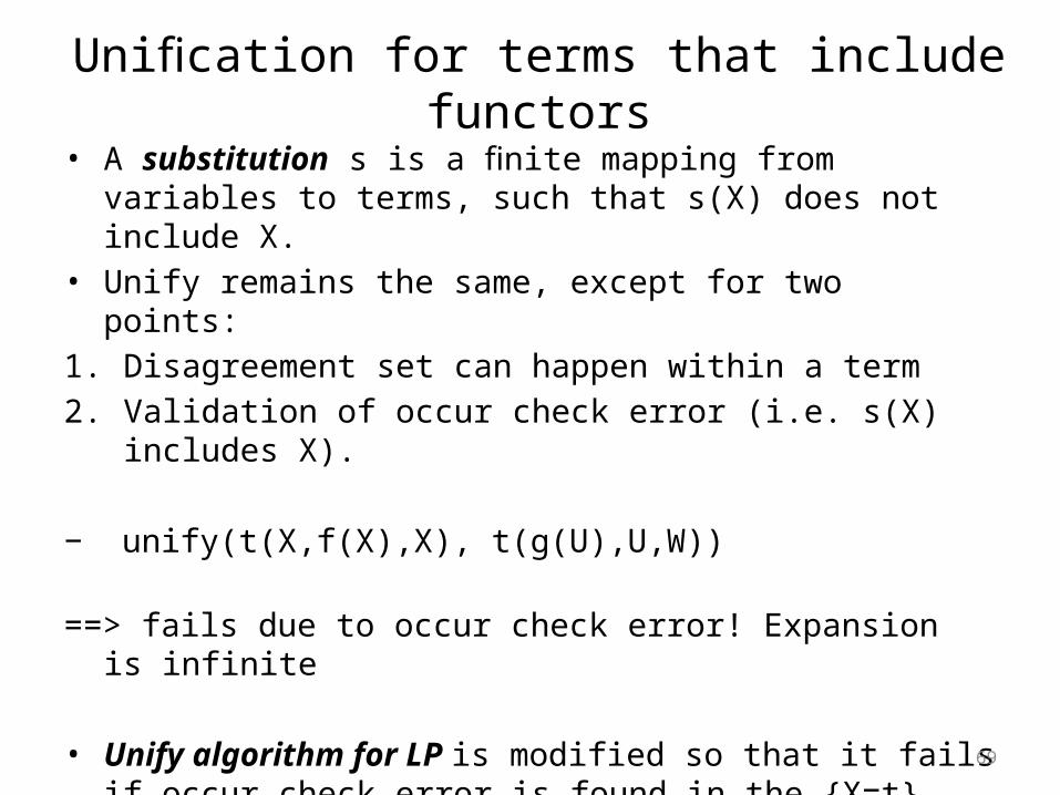
Unification for terms that include functors• A substitution s is a finite mapping from variables to terms, such
that s(X) does not include X. • Unify remains the same, except for two points: 1. Disagreement set can happen within a term
- unify(member(X,tree(X,Left,Right)) , member(Y,tree(9,void,tree(3,void,void))))==> {Y=9, X=9, Left=void, Right=tree(3,void,void)}
− unify(t(X, f(a),X), t(g(U),U,W))==> {X=g(f(a)), U=f(a), W=g(f(a))}
69
Unification for terms that include functors• A substitution s is a finite mapping from variables to terms, such
that s(X) does not include X. • Unify remains the same, except for two points: 1. Disagreement set can happen within a term2. Validation of occur check error (i.e. s(X) includes X).
− unify(t(X,f(X),X), t(g(U),U,W))
==> fails due to occur check error! Expansion is infinite
• Unify algorithm for LP is modified so that it fails if occur check error is found in the {X=t} substitution at the disagreement-set.
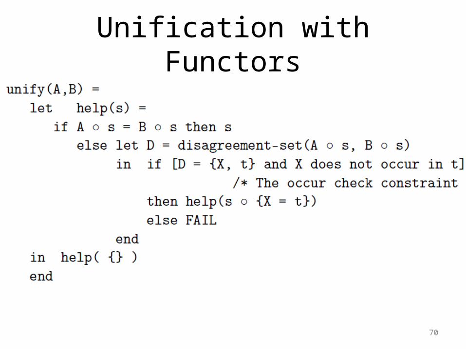
70
Unification with Functors
71
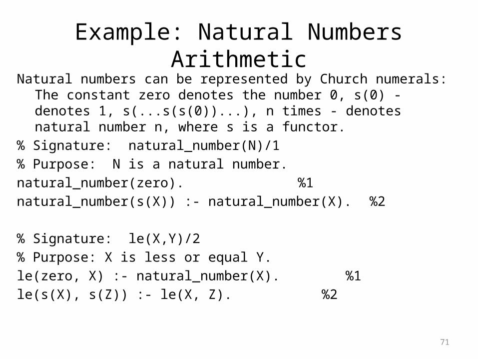
Example: Natural Numbers ArithmeticNatural numbers can be represented by Church numerals: The constant zero
denotes the number 0, s(0) - denotes 1, s(...s(s(0))...), n times - denotes natural number n, where s is a functor.
% Signature: natural_number(N)/1% Purpose: N is a natural number.natural_number(zero). %1natural_number(s(X)) :- natural_number(X). %2
% Signature: le(X,Y)/2% Purpose: X is less or equal Y.le(zero, X) :- natural_number(X). %1le(s(X), s(Z)) :- le(X, Z). %2
72
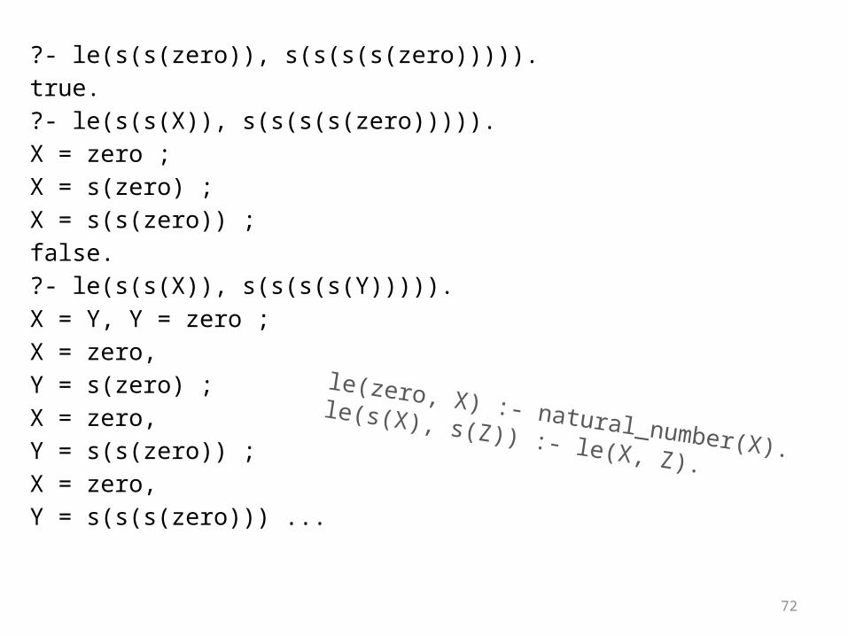
?- le(s(s(zero)), s(s(s(s(zero))))).true.?- le(s(s(X)), s(s(s(s(zero))))).X = zero ;X = s(zero) ;X = s(s(zero)) ;false.?- le(s(s(X)), s(s(s(s(Y))))).X = Y, Y = zero ;X = zero,Y = s(zero) ;X = zero,Y = s(s(zero)) ;X = zero,Y = s(s(s(zero))) ...
le(zero, X) :- natural_number(X).
le(s(X), s(Z)) :- le(X, Z).
73
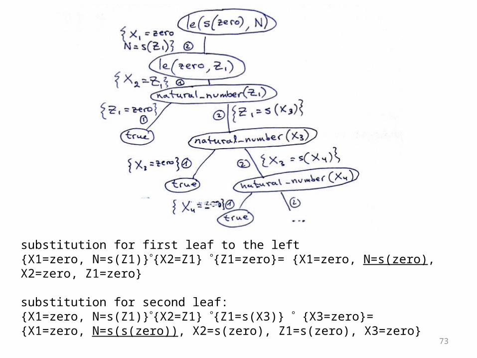
substitution for first leaf to the left{X1=zero, N=s(Z1)}{X2=Z1} {Z1=zero}= {X1=zero, N=s(zero), X2=zero, Z1=zero}
substitution for second leaf:{X1=zero, N=s(Z1)}{X2=Z1} {Z1=s(X3)} {X3=zero}= {X1=zero, N=s(s(zero)), X2=s(zero), Z1=s(zero), X3=zero}
74
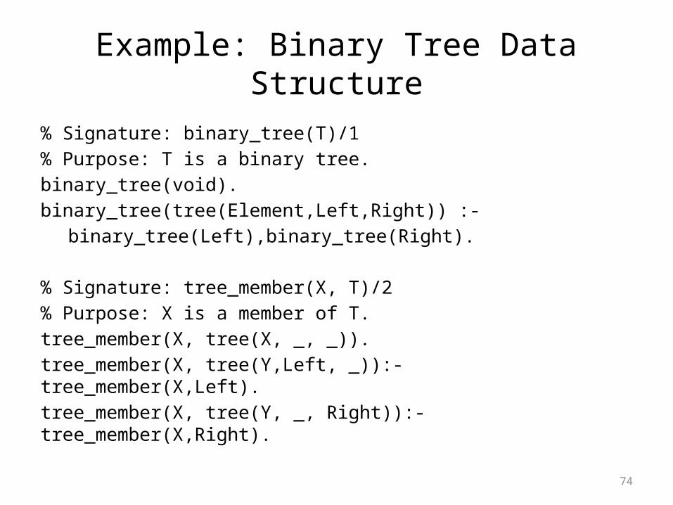
Example: Binary Tree Data Structure
% Signature: binary_tree(T)/1% Purpose: T is a binary tree.binary_tree(void).binary_tree(tree(Element,Left,Right)) :-
binary_tree(Left),binary_tree(Right).
% Signature: tree_member(X, T)/2% Purpose: X is a member of T.tree_member(X, tree(X, _, _)).tree_member(X, tree(Y,Left, _)):- tree_member(X,Left).tree_member(X, tree(Y, _, Right)):- tree_member(X,Right).
75
Summary
• Proof tree types• LP with functors• Unify + occur check error
76
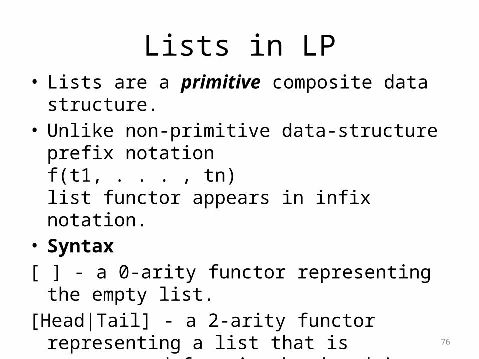
Lists in LP• Lists are a primitive composite data structure.• Unlike non-primitive data-structure prefix notation
f(t1, . . . , tn)list functor appears in infix notation.
• Syntax[ ] - a 0-arity functor representing the empty list.[Head|Tail] - a 2-arity functor representing a list that is
constructed from its head and its tail, where the tail is also a list.
77
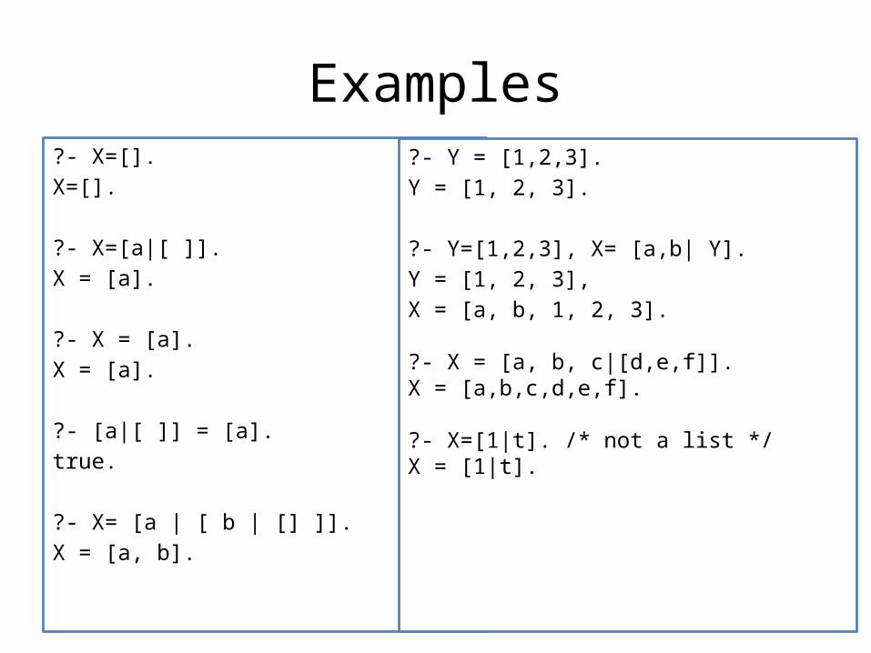
Examples?- X=[].X=[].
?- X=[a|[ ]].X = [a].
?- X = [a]. X = [a].
?- [a|[ ]] = [a].true.
?- X= [a | [ b | [] ]].X = [a, b].
?- Y = [1,2,3].Y = [1, 2, 3].
?- Y=[1,2,3], X= [a,b| Y].Y = [1, 2, 3],X = [a, b, 1, 2, 3].
?- X = [a, b, c|[d,e,f]].X = [a,b,c,d,e,f].
?- X=[1|t]. /* not a list */X = [1|t].

78
LP lists - List membership% Signature: member(X, List)/2% Purpose: X is a member of List.member(X, [X|Xs]).member(X, [Y|Ys]) :- member(X, Ys).
% checks membership?- member(a, [b,c,a,d]). % takes an element from a list?- member(X, [b,c,a,d]). % generates a list containing b?- member(b, Z).
79
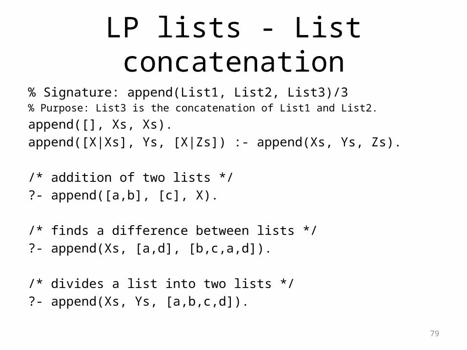
LP lists - List concatenation% Signature: append(List1, List2, List3)/3% Purpose: List3 is the concatenation of List1 and List2.
append([], Xs, Xs).append([X|Xs], Ys, [X|Zs]) :- append(Xs, Ys, Zs).
/* addition of two lists */?- append([a,b], [c], X).
/* finds a difference between lists */?- append(Xs, [a,d], [b,c,a,d]).
/* divides a list into two lists */?- append(Xs, Ys, [a,b,c,d]).

80
append([], Xs, Xs). %1append([X|Xs], Ys, [X|Zs] ) :- append(Xs, Ys, Zs).%2
append(Xs, [a,d], [b,c,a,d])
append(Xs1, [a,d], [c,a,d])
2{Xs=[X1|Xs1], Ys1=[a,d],X1=bZs1=[c,a,d]}
true
2{Xs1=[X2|Xs2], Ys2=[a,d],X2=cZs2=[a,d]}
append(Xs2, [a,d], [a,d])2{Xs2=[X3|Xs3], Ys3=[a,d],X3=aZs3=[d]}
1{Xs2=[], Xs3=[a,d]}
append(Xs3, [a,d], [d])
2{Xs3=[X4|Xs4], Ys4=[a,d],X4=dZs4=[]}
append(Xs4, [a,d], [])
fail
81
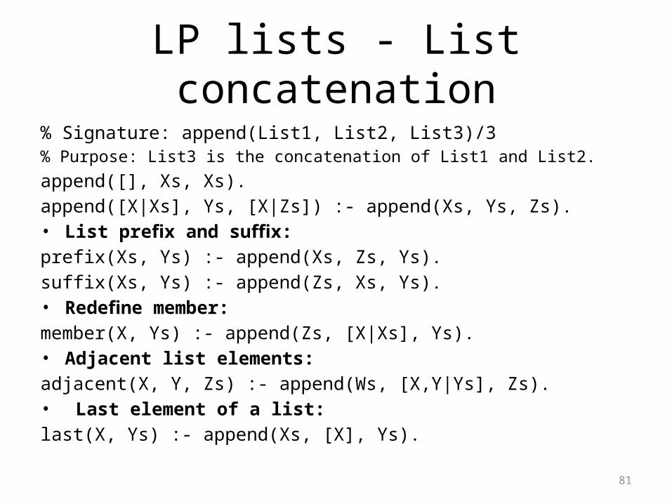
LP lists - List concatenation% Signature: append(List1, List2, List3)/3% Purpose: List3 is the concatenation of List1 and List2.
append([], Xs, Xs).append([X|Xs], Ys, [X|Zs]) :- append(Xs, Ys, Zs).• List prefix and suffix:prefix(Xs, Ys) :- append(Xs, Zs, Ys).suffix(Xs, Ys) :- append(Zs, Xs, Ys).• Redefine member:member(X, Ys) :- append(Zs, [X|Xs], Ys).• Adjacent list elements:adjacent(X, Y, Zs) :- append(Ws, [X,Y|Ys], Zs).• Last element of a list:last(X, Ys) :- append(Xs, [X], Ys).
82
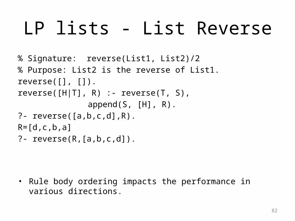
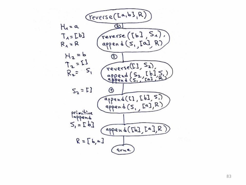
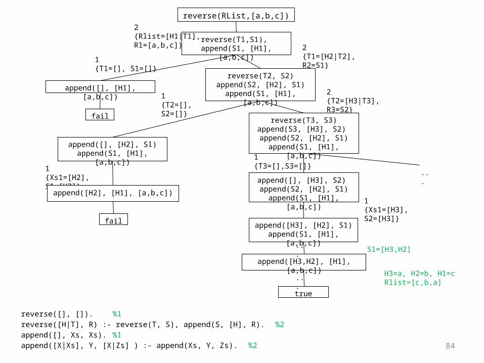
LP lists - List Reverse% Signature: reverse(List1, List2)/2% Purpose: List2 is the reverse of List1.reverse([], []).reverse([H|T], R) :- reverse(T, S),
append(S, [H], R).?- reverse([a,b,c,d],R).R=[d,c,b,a]?- reverse(R,[a,b,c,d]).
• Rule body ordering impacts the performance in various directions.
83
84
reverse([], []). %1reverse([H|T], R) :- reverse(T, S), append(S, [H], R). %2append([], Xs, Xs). %1append([X|Xs], Y, [X|Zs] ) :- append(Xs, Y, Zs). %2
reverse(RList,[a,b,c])
reverse(T1,S1), append(S1, [H1], [a,b,c])
2{Rlist=[H1|T1],R1=[a,b,c]} 2
{T1=[H2|T2], R2=S1}
fail
1{T2=[], S2=[]}
reverse(T3, S3)append(S3, [H3], S2) append(S2, [H2], S1)
append(S1, [H1], [a,b,c])
1{T1=[], S1=[]}
append([], [H1], [a,b,c])
reverse(T2, S2)append(S2, [H2], S1)
append(S1, [H1], [a,b,c])
append([], [H2], S1) append(S1, [H1], [a,b,c])
1{Xs1=[H2], S1=[H2]}
append([H2], [H1], [a,b,c])
fail
2{T2=[H3|T3], R3=S2}
1{T3=[],S3=[]}
append([], [H3], S2) append(S2, [H2], S1)
append(S1, [H1], [a,b,c]) 1{Xs1=[H3], S2=[H3]}
append([H3], [H2], S1)append(S1, [H1], [a,b,c])
true
append([H3,H2], [H1], [a,b,c])
... S1=[H3,H2]
... H3=a, H2=b, H1=cRlist=[c,b,a]
...
85
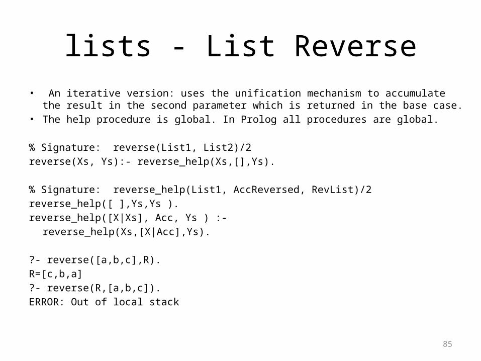
lists - List Reverse• An iterative version: uses the unification mechanism to accumulate the result in the second
parameter which is returned in the base case. • The help procedure is global. In Prolog all procedures are global.
% Signature: reverse(List1, List2)/2reverse(Xs, Ys):- reverse_help(Xs,[],Ys).
% Signature: reverse_help(List1, AccReversed, RevList)/2reverse_help([ ],Ys,Ys ).reverse_help([X|Xs], Acc, Ys ) :-
reverse_help(Xs,[X|Acc],Ys).
?- reverse([a,b,c],R).R=[c,b,a]?- reverse(R,[a,b,c]).ERROR: Out of local stack
87
The Cut Operator - Pruning Trees
The cut system predicate, denoted !, is a Prolog built-in predicate, for pruning proof trees.
• avoiding traversing failed sub-trees.• eliminates wrong answers or infinite branches
88
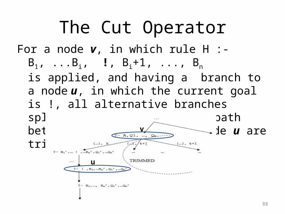
The Cut OperatorFor a node v, in which rule H :- B1, ...Bi, !, Bi+1, ..., Bn
is applied, and having a branch to a node u, in which the current goal is !, all alternative branches splitting from nodes in the path between v (including) and node u are trimmed.
v
u
89
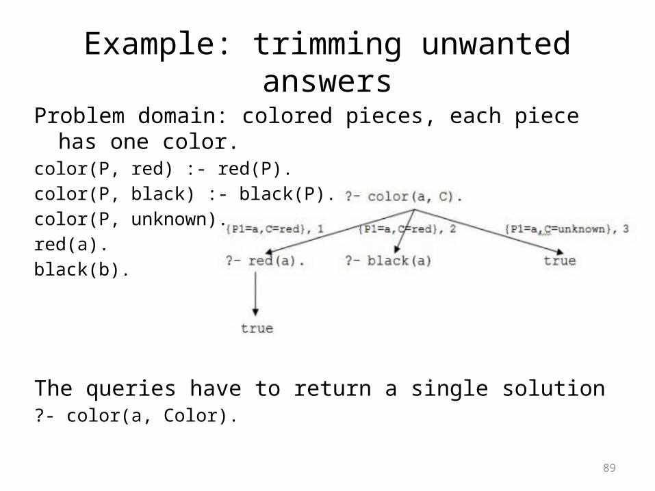
Example: trimming unwanted answersProblem domain: colored pieces, each piece has one color.color(P, red) :- red(P).color(P, black) :- black(P).color(P, unknown).red(a).black(b).
The queries have to return a single solution?- color(a, Color).
90
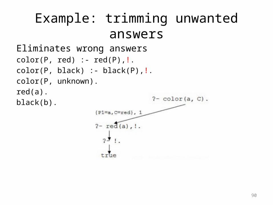
Example: trimming unwanted answersEliminates wrong answerscolor(P, red) :- red(P),!.color(P, black) :- black(P),!.color(P, unknown).red(a).black(b).
91
Example: avoiding unnecessary searches (duplicate answers)
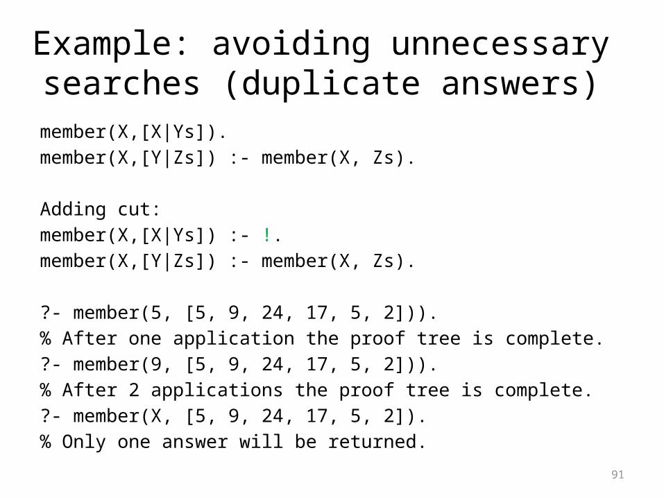
member(X,[X|Ys]). member(X,[Y|Zs]) :- member(X, Zs).
Adding cut:member(X,[X|Ys]) :- !. member(X,[Y|Zs]) :- member(X, Zs).
?- member(5, [5, 9, 24, 17, 5, 2])). % After one application the proof tree is complete.?- member(9, [5, 9, 24, 17, 5, 2])). % After 2 applications the proof tree is complete.?- member(X, [5, 9, 24, 17, 5, 2]). % Only one answer will be returned.
92
Red & Green Cuts
• Green: Only optimize the search• Red: Does not compute the intended relation
(Don’t look for color in the code… it’s a matter of semantics)
93
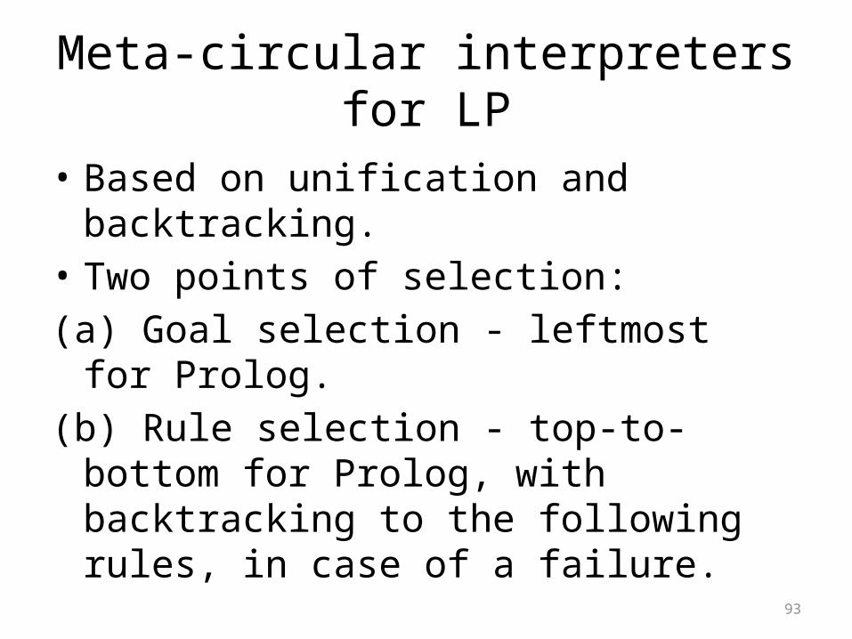
Meta-circular interpreters for LP
• Based on unification and backtracking.• Two points of selection:(a) Goal selection - leftmost for Prolog.(b) Rule selection - top-to-bottom for Prolog,
with backtracking to the following rules, in case of a failure.
94
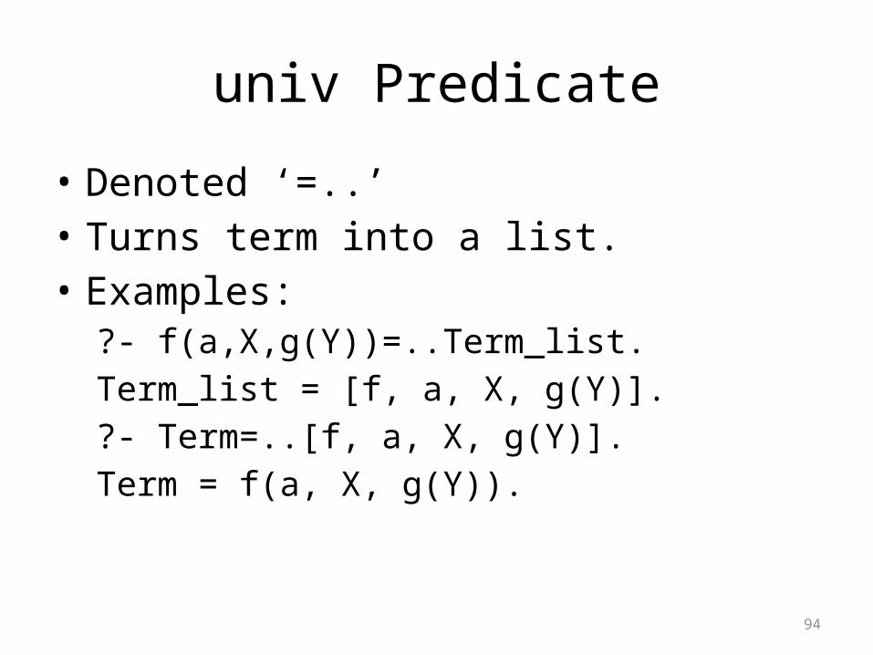
univ Predicate
• Denoted ‘=..’• Turns term into a list.• Examples:
?- f(a,X,g(Y))=..Term_list.Term_list = [f, a, X, g(Y)].?- Term=..[f, a, X, g(Y)].Term = f(a, X, g(Y)).
95
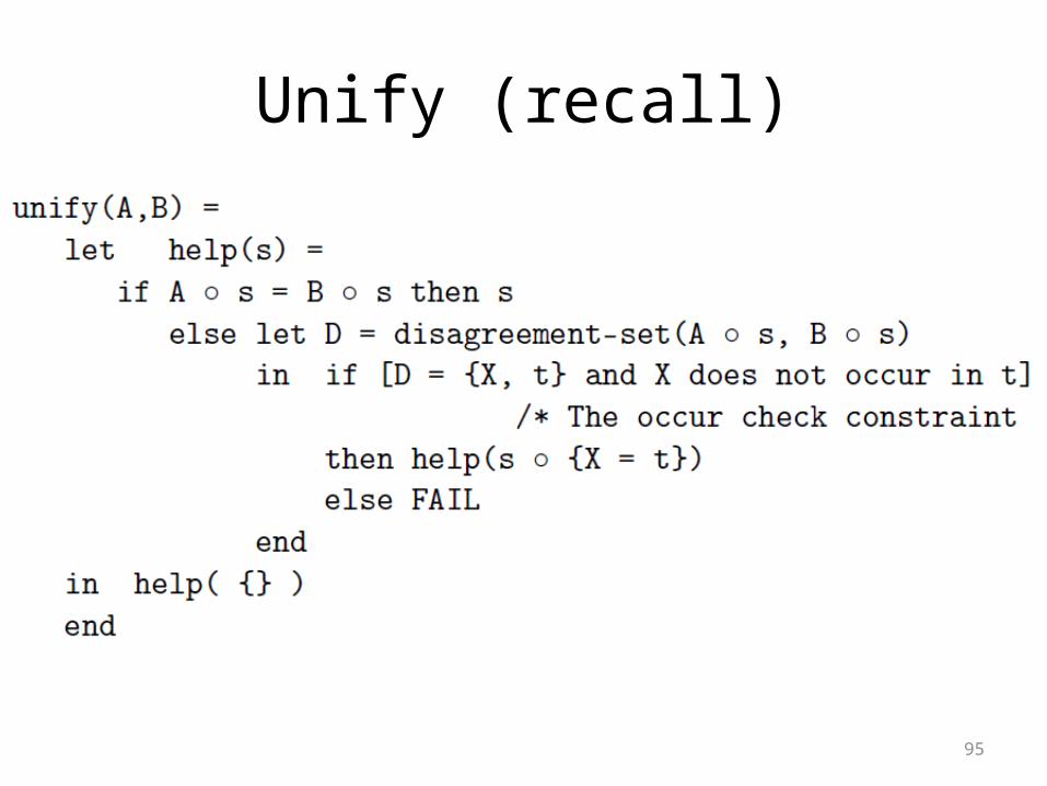
Unify (recall)

96
Unify
In order to implement it we need to distinguish between variables and constants.
Our implementation: constants denoting variables are distinguished from true constants.For example:c(f(X), G,X), c(G, Y, f(d)) => c(f(x), g, x), c(g, y, f(d))
97
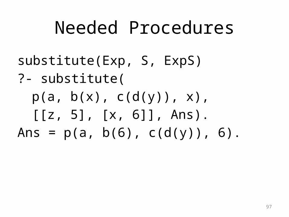
Needed Procedures
substitute(Exp, S, ExpS)?- substitute(
p(a, b(x), c(d(y)), x), [[z, 5], [x, 6]], Ans).
Ans = p(a, b(6), c(d(y)), 6).

98
Needed Procedures
disagreement(A, B, Set)?- disagreement(
p(x,y)p(x,5), Set)
Set = [y,5]
99
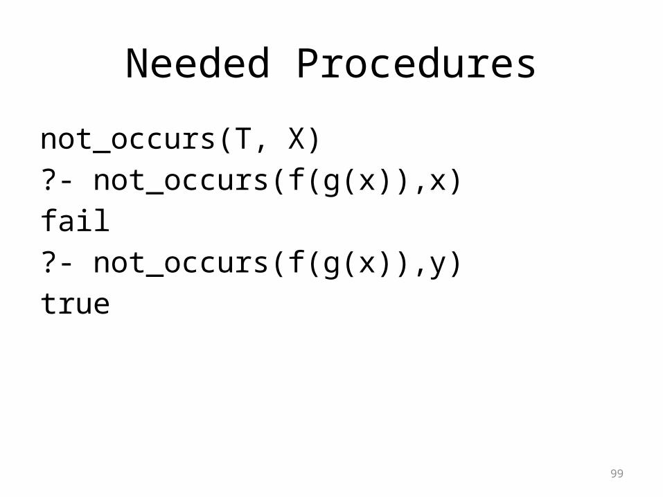
Needed Procedures
not_occurs(T, X)?- not_occurs(f(g(x)),x)fail?- not_occurs(f(g(x)),y)true
100
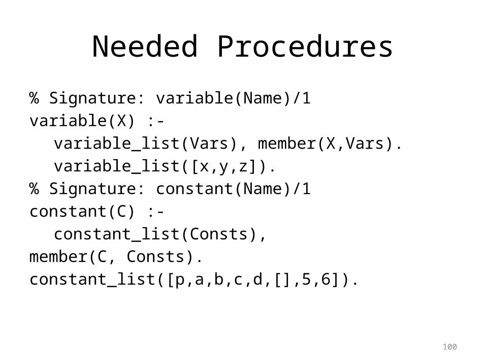
Needed Procedures
% Signature: variable(Name)/1variable(X) :-
variable_list(Vars), member(X,Vars).variable_list([x,y,z]).
% Signature: constant(Name)/1constant(C) :-
constant_list(Consts), member(C, Consts).constant_list([p,a,b,c,d,[],5,6]).
101
Needed Procedures
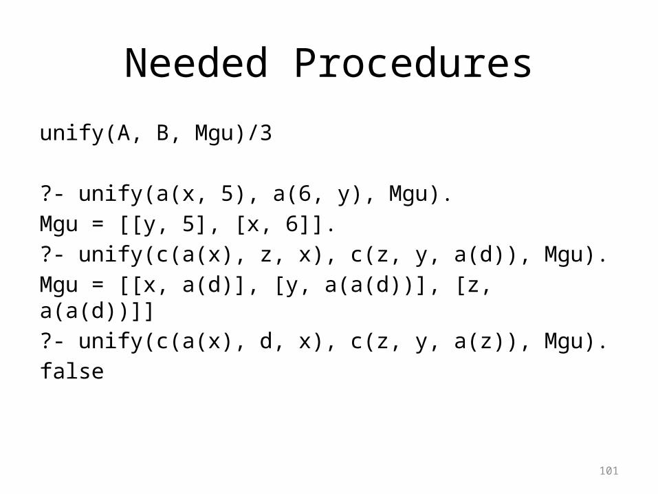
unify(A, B, Mgu)/3
?- unify(a(x, 5), a(6, y), Mgu).Mgu = [[y, 5], [x, 6]].?- unify(c(a(x), z, x), c(z, y, a(d)), Mgu).Mgu = [[x, a(d)], [y, a(a(d))], [z, a(a(d))]]?- unify(c(a(x), d, x), c(z, y, a(z)), Mgu).false

102
Meta Circular Interpreter for LP
• Based on unification and backtracking• Main Procedure is called solve (queries are
presented to it)• Need pre-processing (next slide)
103
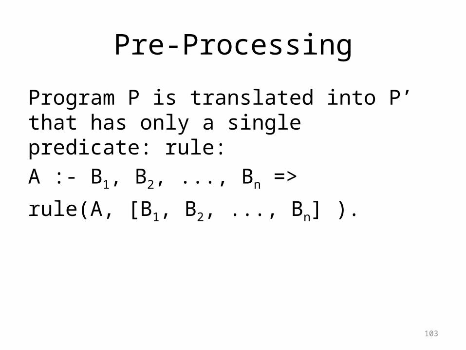
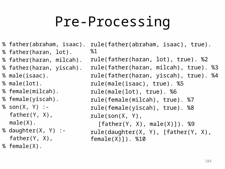
Pre-Processing
Program P is translated into P’ that has only a single predicate: rule:A :- B1, B2, ..., Bn =>
rule(A, [B1, B2, ..., Bn] ).
104
Pre-Processing% father(abraham, isaac).% father(haran, lot).% father(haran, milcah).% father(haran, yiscah).% male(isaac).% male(lot).% female(milcah).% female(yiscah).% son(X, Y) :-
father(Y, X),male(X).
% daughter(X, Y) :- father(Y, X),
% female(X).
rule(father(abraham, isaac), true). %1rule(father(haran, lot), true). %2rule(father(haran, milcah), true). %3rule(father(haran, yiscah), true). %4rule(male(isaac), true). %5rule(male(lot), true). %6rule(female(milcah), true). %7rule(female(yiscah), true). %8rule(son(X, Y),
[father(Y, X), male(X)]). %9rule(daughter(X, Y), [father(Y, X), female(X)]). %10
105
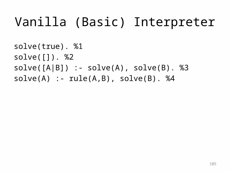
Vanilla (Basic) Interpreter
solve(true). %1solve([]). %2solve([A|B]) :- solve(A), solve(B). %3solve(A) :- rule(A,B), solve(B). %4
106
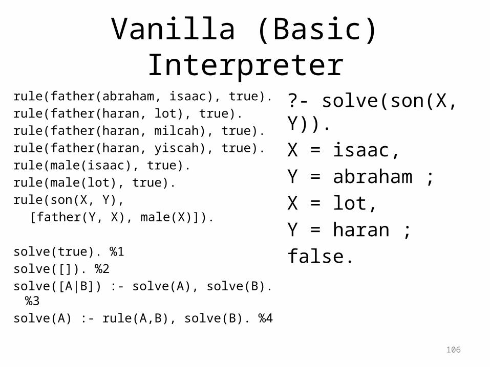
Vanilla (Basic) Interpreterrule(father(abraham, isaac), true). rule(father(haran, lot), true).rule(father(haran, milcah), true).rule(father(haran, yiscah), true).rule(male(isaac), true).rule(male(lot), true).rule(son(X, Y),
[father(Y, X), male(X)]).
solve(true). %1solve([]). %2solve([A|B]) :- solve(A), solve(B).
%3solve(A) :- rule(A,B), solve(B). %4
?- solve(son(X, Y)).X = isaac,Y = abraham ;X = lot,Y = haran ;false.
107
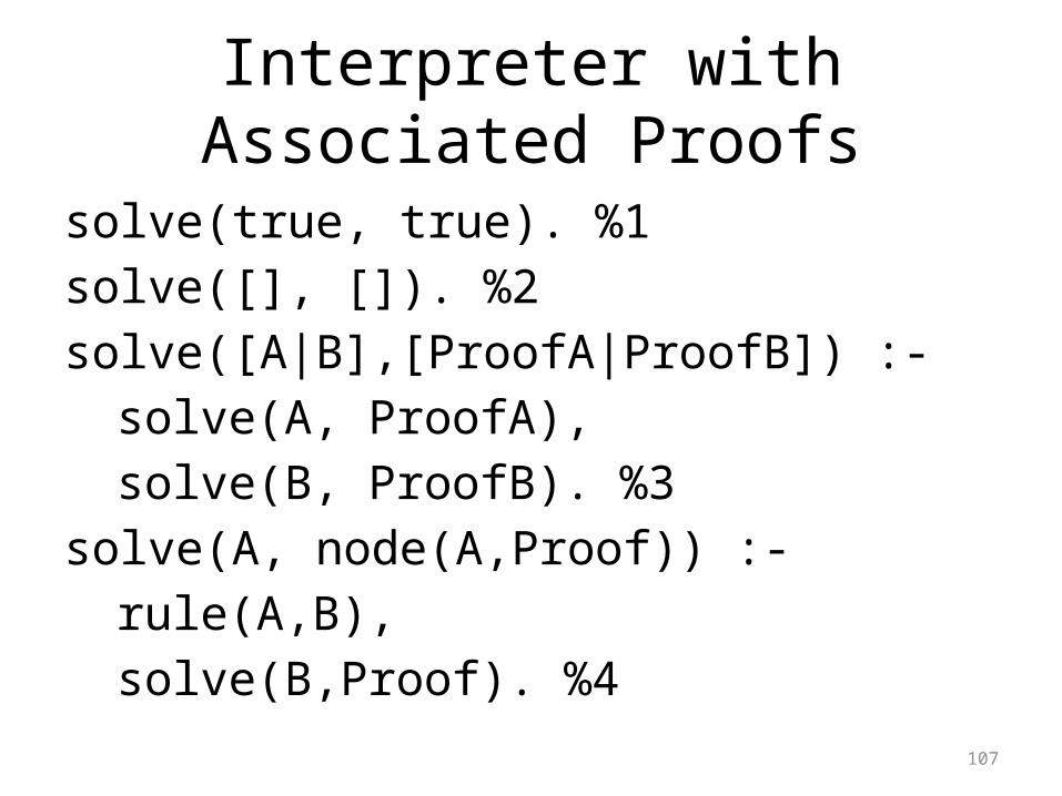
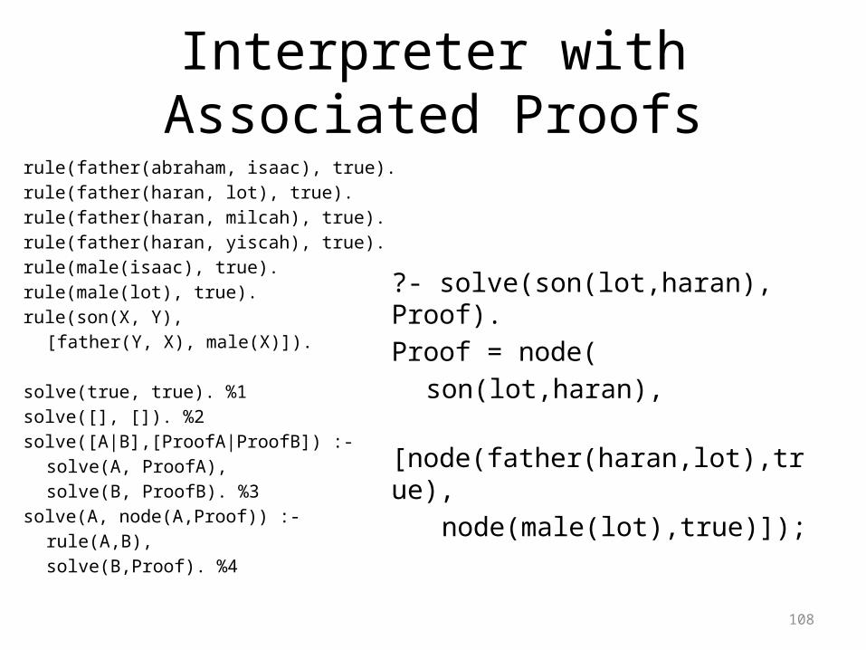
Interpreter with Associated Proofs
solve(true, true). %1solve([], []). %2solve([A|B],[ProofA|ProofB]) :-
solve(A, ProofA), solve(B, ProofB). %3
solve(A, node(A,Proof)) :-rule(A,B), solve(B,Proof). %4
108
Interpreter with Associated Proofsrule(father(abraham, isaac), true). rule(father(haran, lot), true).rule(father(haran, milcah), true).rule(father(haran, yiscah), true).rule(male(isaac), true).rule(male(lot), true).rule(son(X, Y),
[father(Y, X), male(X)]).
solve(true, true). %1solve([], []). %2solve([A|B],[ProofA|ProofB]) :-
solve(A, ProofA), solve(B, ProofB). %3
solve(A, node(A,Proof)) :-rule(A,B), solve(B,Proof). %4
?- solve(son(lot,haran), Proof).Proof = node(
son(lot,haran),
[node(father(haran,lot),true),
node(male(lot),true)]);
109
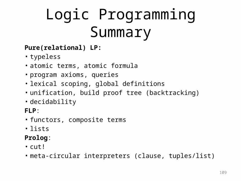
Logic Programming SummaryPure(relational) LP: • typeless• atomic terms, atomic formula• program axioms, queries• lexical scoping, global definitions• unification, build proof tree (backtracking)• decidabilityFLP: • functors, composite terms• listsProlog: • cut!• meta-circular interpreters (clause, tuples/list)